author's personal copy - technion

This article appeared in a journal published by Elsevier. The attachedcopy is furnished to the author for internal non-commercial researchand education use, including for instruction at the authors institution

and sharing with colleagues.

Other uses, including reproduction and distribution, or selling orlicensing copies, or posting to personal, institutional or third party

websites are prohibited.

In most cases authors are permitted to post their version of thearticle (e.g. in Word or Tex form) to their personal website orinstitutional repository. Authors requiring further information

regarding Elsevier’s archiving and manuscript policies areencouraged to visit:

http://www.elsevier.com/copyright

http://www.elsevier.com/copyright

Author's personal copy

Flexural vibration patterning using an array of actuators

Eyal Setter, Izhak Bucher n

Technion, Israel Institute of Technology, Faculty of Mechanical Engineering, Technion, Haifa 32000, Israel

a r t i c l e i n f o

Article history:

Received 1 November 2009

Received in revised form

5 July 2010

Accepted 25 September 2010

Handling Editor: A.V. MetrikineAvailable online 23 October 2010

a b s t r a c t

This paper describes a method to create unique vibration patterns by means of an array

of actuators acting on the boundaries of the controlled structure. The method builds, in

an iterative process, a black-box model by employing a series of probing external

excitation vectors. Once a model has been identified, an optimization stage seeks the

dynamic force-vector that generates the best approximation for a specified deformation

pattern. Among the obtainable periodic responses are standing or travelling flexural

waves of single or multi-frequencies in one or two spatial dimensions, as well as

rotating, vortex-like, flexural waves in 2D. The paper describes the force-tuning process

through which dozens of actuators can be modified automatically until the response,

measured at hundreds of sensed locations, complies with the anticipated response. The

excitation that yields the desired response is calculated using an over-determined set of

least-squares equations that approximates the inverse of the identified model. The

precise iterative tuning process can overcome some nonlinearity, manifested by

additional harmonics in the response, by injecting forces that nullify their effect.

Methods for wavelength optimization and wave identification in 1D and 2D are also

discussed. The proposed tuning method showed good results in numerical simulation

and in real world experiments.

& 2010 Elsevier Ltd. All rights reserved.

1. Introduction

Shaping the vibration pattern of a given finite, continuous structure using external forces can be useful in several cases.For example, one desired vibration pattern is a travelling flexural wave of predetermined wavelength, amplitude, direction,and phase. Such a pattern is often used to generate propulsion, as in squeeze-film levitation and transportation devices[1,2], where a travelling pressure wave carries a levitated object. In robotics, snake-like structures make use of travellingwave movements for propulsion over solid surfaces [3], or in steering and maneuvering in a viscous fluid environment [4].Travelling waves are also used to absorb incoming vibration in robotic arms [5]. An active vibration control method dealingwith waves is investigated in [6,7] with implementation on a flexible beam and a flexible plate, respectively. The controlaims to eliminate vibration modes by cancelling reflected or transmitted waves. While [5–7] aim to suppress undesiredvibration, the current paper suggests a method to excite desired structural responses, such as travelling waves, whileconstructing a non-modal, measurements-based system model. Ultrasonic motors are a relatively recent and uniqueapplication that makes use of high frequency, short wavelength travelling flexural waves to achieve accurate and relativelyhigh torque positioning without the need for reduction gears [8,9]. In micro-electro-mechanical systems (MEMS)applications, non-circular structures are preferable in batch micro-machining of silicon. In such application, the need arises

Contents lists available at ScienceDirect

journal homepage: www.elsevier.com/locate/jsvi

Journal of Sound and Vibration

0022-460X/$ - see front matter & 2010 Elsevier Ltd. All rights reserved.

doi:10.1016/j.jsv.2010.09.027

n Corresponding author. Tel.: +972 4 8293153; fax: +972 4 8295711.

E-mail address: [email protected] (I. Bucher).

Journal of Sound and Vibration 330 (2011) 1121–1140


to generate rotating flexural waves in a rectangular plate that performs as the stator of a micro-ultrasonic motor. Suchwaves have been generated in square micro-plates by dual- or multimode excitation [10]. A similar approach to creatingtravelling waves in rectangular structures using single-phase actuation was introduced in [11]. For a theoretical derivationof a circumferential force distribution that yields travelling waves in one- and two-dimensional structures by means ofinfinite modal summation, see [12]. Another example of motion tuning is the use of rigidly oscillating plates that slide andorient parts on assembly lines by friction-induced velocity or force fields [13]. In this example, the rigid plate has sixdegrees of freedom and is controlled by six actuators. In other cases, elastic stretching platforms are used in growingin-vitro human heart tissues to better simulate their natural habitat and hence improve functionality of the artificiallygrown cells [14]. Vortex structural and acoustic power flows were analyzed by Tanaka et al. [15] for simply supported thinelastic plate under feed-forward vibration control. The vortexes, described as interference between modes of vibrationwere observed when two modes of vibration were affected. The method proposed in the present work allows an extendedfreedom in determining the vortex geometry (wavelengths, frequency, and location) but, clearly the method in [15] wouldyield larger amplitudes of vibration under fixed excitation level due to the proximity of the excitation frequencies toresonance. The present method is broader in scope due to its ability to tune arbitrary vibration patterns, for apredetermined set of actuators distributed only around the boundaries. The present method contrary to [14] uses a modelthat does not rely on specific vibration modes, under the assumption that multiple modes of vibration can play a significantrole when attempting to generate a propagating phenomenon [12].

Nevertheless, to the best of our knowledge, no studies have yet considered the tuning of a given elastic structure’sresponse in a variety of vibration patterns, including standing, travelling, single or multi-frequencies waves in one or twospatial dimensions, and rotating waves in 2D. In the current study, multi-input multi-output (MIMO) tuning experimentsare conducted, with as many as 32 actuators and over 500 sensed locations (in tuning out-of-plane vibrationexperimentally on a membrane). The proposed method is based on extending the procedure presented in [16] to a non-square system having a large number of sensors and actuators. Furthermore, in contrast to [16], which essentiallycontrolled a single node on a shaft, the present study is employed to experimentally control the steady-state vibrations ofan entire region on a structure.

The following section describes the problem and the proposed method. The basic approach and the underlying stagesare outlined in Section 2.1, followed by the mathematical description of a typical desired response in Section 2.2. Handlingnonlinearities is referred to in Section 2.3, and the determination of the optimal wavelength is explained in Section 2.4.Wave identification methods are reviewed in Section 2.5. Numerical and experimental results come next. The experimentlayout is presented in Section 3.1. Simulated and experimental results of 1D string and 2D membrane models are given inSections 3.2 and 3.3, respectively. The paper ends with concluding notes in Section 4, where the merits of the proposedmethod are outlined.

2. Model identification and inversion

This section outlines the mathematical foundation of the proposed tuning method. The tuning process, as illustrated inFig. 1, begins with system identification. Next, the optimal wavelength for a given excitation frequency is found, and given

Fig. 1. The proposed tuning method scheme.

E. Setter, I. Bucher / Journal of Sound and Vibration 330 (2011) 1121–11401122


the system model, the excitation needed to yield the desired response is calculated. When the device under test exhibits amild nonlinearity, additional perturbations are added to an extended model allowing for multi-frequency tuning thateliminate parasitic harmonics. The section ends with a short description of wave identification methods. It should be notedthat Sections 2.1, 2.3 and 2.5 include previous works, which set the ground for the introduction of the newly developedconcepts as given in Sections 2.2 and 2.4, and for the analysis of the results in Section 3.

2.1. Method in brief

The proposed method is based on a procedure presented in [16]. The following discussion briefly reviews this procedureand further develops it for real-world multi-output multi-input (MIMO) systems and various vibration patterns basedupon new interpretations and physical findings. The proposed method aims to find the excitation parameters under whicha desired structural response in terms of a specified spatial vibration pattern, e.g., travelling flexural waves is obtained. Themethod uses only measured response data with almost no previous knowledge of the system at hand. The sensors andactuators should be placed at suitable locations. If they are not, the proposed method can detect any deficiency or inferiordeployment of the transducers. By means of the proposed enhancements, the algorithm can find the best achievableresponse within a family of desired patterns (e.g. travelling waves).

The proposed method will be regarded in this text as means of tuning flexural (transverse) steady state, out of planedisplacements of string and membrane models. Fig. 2(a) depicts an example of an abstract structure (a membrane) excitedby several actuators. The flexural vibration (out of plane displacement) is measured at certain points for a random set oforthonormal excitation vectors. Fig. 2(b) shows the same structure after the tuning process, where the structure isexperiencing the desired vibration pattern.

Let us consider a system with N measured points andM exciters. The theoretical system can be described in a spatiallydiscrete fashion (e.g., finite element—FE derived model):

M €gþC _gþKg¼ Bcðg,tÞ, g 2 RN�1, c 2 RM�1, M,C,K 2 RN�N , B 2 RN�M, (1)

where g is the state vector of generalized coordinates representing the structural deformations, and c(g,t)=c0(t)+c1(g,t) isthe time-dependent input vector or the excitation, containing the directly influenced part c0(t), and some mildnonlinearities c1(g,t) that are state-vector dependent. M, C, K are the mass, damping, and stiffness matrices, respectively,and B is a matrix of force distribution weighting, mapping the excitation vector to the appropriate degrees of freedom.

The proposed method adapts the external excitation vector c0(t) to obtain a desired response pattern manifested by g inEq. (1). The current paper focuses on steady-state time periodic vibrations, but not necessarily on pure sinusoids. Theassumption of steady-state time periodic vibrations converts the differential equation (Eq. (1)) into a system of algebraicequations. The force adaptation process begins with a black-box model identification stage. In this stage, a set ofindependent excitation vectors is generated, the corresponding response vectors are measured, and thus the model isformed.

For a perfectly linear system, running all the exciters at the same frequency, o0, yields two types of distinguishingparameters per exciter—amplitude and phase. A frequency index h must be added to achieve a multi-frequency response,or if nonlinear super- and sub-harmonics are expected. The mth exciter induces a force comprised of several harmonics, i.e.

qm ¼XPh ¼ 1

qhm, m¼ 1,2,. . .,M, (2)

where qhm ¼Qh

m cosðhx0tÞþRhm sinðhx0tÞ, h¼ 1,2,. . .,P.

Fig. 2. (a) Vibrating structure at some t=t0, before tuning the response and (b) same structure experiencing tuned vibration of a travelling flexural

wave at t=t1.

E. Setter, I. Bucher / Journal of Sound and Vibration 330 (2011) 1121–1140 1123


Here 9Qhmþ iRh

m9, (i�ffiffiffiffiffiffiffi�1p

) represents the force amplitude at the mth excitation point. This component has excitationfrequency ho0 (rad/s), and its phase is dictated by argðQh

mþ iRhmÞ relative to a common reference. Hence, Qh

m,Rhm are tunable

parameters.For the model identification stage, M exciters require an excitation basis of 2M� 2M parameters per frequency.

Accordingly, the system’s measured response at the nth point n¼ 1,2,. . .,Nð Þ to the rth r¼ 1,2,. . .,2Mð Þ excitation vector ofthe hth frequency component is

ahr,n ¼ Ah

r,n cosðhx0tÞþBhr,n sinðhx0tÞ: (3)

The force amplitude of the mth exciter of the rth excitation vector of the hth frequency component is

qhr,m ¼Qh

r,m cosðhx0tÞþRhr,m sinðhx0tÞ: (4)

When Eqs. (3) and (4) are combined for the entire system and rearranged by the coefficients of cos(ho0t), sin(ho0t),the result is the following set of equations per frequency component (for a single harmonic index h):

Ar,1

^

Ar,N

Br,1

^

Br,N

0BBBBBBBBB@

1CCCCCCCCCA¼

H1,1 H1,2M

&

Hn,m

&

H2N ,1 � � � H2N ,2M

0BBBBBBBBB@

1CCCCCCCCCA

Qr,1

^

Qr,M

Rr,1

^

Rr,M

0BBBBBBBBB@

1CCCCCCCCCA

, (5)

where Hn,m represents the system gain of in-phase or in-quadrature components. Eq. (5) can be rewritten morecompactly as

ar ¼Hqr , H 2 R2N�2M, ar 2 R2N�1, qr 2 R

2M�1, (6)

where ar is the response vector (left-hand side of Eq. (5)), and qr holds the components of the rth excitation vector (columnvector in the right-hand side of Eq. (5)). Combining the responses for all r¼ 1,2,. . .,2M excitation vectors gives

A¼HQ , A 2 R2N�2M, Q 2 R2M�2M, (7)

where A is the response matrix consisting of the columns ar, H is the system model, and qr, the corresponding excitationvectors filling the columns of Q.

The receptance of a perfectly linear system with frequency response matrix derived from Eq. (1) can be written as

aðx0Þ9 �x20Mþ ix0CþK

� ��1B, aðx0Þ 2 R

N�M: (8)

For such a system (see [16]), the model matrix H used in Eqs. (6) and (7) takes the form

(9)

where the dashed line indicates matrix partitioning. Clearly, even the slightest nonlinearity will sometimes distort thestructure of Eq. (9). Because the excitation basis, Q, was chosen to be orthonormal, the system model can be numericallyestimated without matrix inversion

H¼AQ -1¼AQ T: (10)

Once the model has been found, Eq. (6) can now be inverted in order to find the required force-vector yielding a desiredresponse. Normally, there are more sensors than actuators ðN4MÞ. Therefore, an over-determined least squares strategyis adopted to calculate the excitation vector – qd that will result in the most suitable response vector – ad with a minimumerror norm [17–19]. Based upon Eqs. (6), (7) and (10), and assuming that the response matrix A has full rank, it is possibleto calculate a unique solution for the excitation by pseudo-inversion of A

qd ¼Hyad ¼Q Ayad, (11)

where the operator ( � )y stands for pseudo-inverse, and ad represents the desired spatial solution. The singular valuedecomposition (SVD) can be adopted to carry out the numerical computation [18].

The proposed tuning method can be used to assess the level of system nonlinearity in a particular operation regime byexamining the level of agreement between the measurements-based model matrix H and Eq. (9).



2.2. Describing the appropriate wave response

Suppose ad describes a wave travelling in a certain direction in space. This wave should have a desired wavelength l andwavenumber K,

j¼ 2p=k: (12)

A travelling wave can be represented by

uðx,tÞ ¼ cosðxt�jxÞ ¼ cosxt cosjxþsinxt sinjx: (13)

An array of sensors located at x1,x2,. . .,xN , would, measure a vector of amplitudes that when decomposed into in-phaseand in-quadrature components yields

ad ¼ ð cosjx1 � � � cosjxN sinjx1 � � � sinjxN ÞT, (14)

where xn ðn¼ 1,2,:::,N Þ are the measured points along the structure.Based on Eqs. (11)–(14), it is evident that calculating the excitation forces generating a desired wave form along a

structure depends on the wavelength l. At this stage, only steady-state response at a fixed frequency is taken intoconsideration. Hence, the wavelength depends on the known frequency, and on the unknown properties of the medium.For example, the wavenumber of a taut string conforms to j¼x=c, where o is the vibration frequency. The wave velocityof propagation (phase velocity) c is given by c¼

ffiffiffiffiffiffiffiffiffiT=q

p, where T is the tension and r is the mass density per unit length. Yet

since both the tension and the material properties are unknown, the measured data can be used to discover the optimizedwavelength, as discussed in Section 2.4.

2.3. Extending the method for systems exhibiting mild nonlinearity

As the system in question may not always obey strict linearity, the solution found using the proposed approach may notbe optimal. An optimized solution for the case of a travelling wave is considered to be a wave of the desired amplitude forthe travelling component and minimal amplitude for the standing component. A general, not necessarily linear system canbe described by

a¼ f ðq,tÞ, (15)

where a is the measured response amplitude and q represents the excitation amplitudes. For a desired response ad, theexcitation qd should be applied. This excitation can be written as qd=q0+dq, where q0 is the initial guess or solutionachieved using the proposed linear algorithm, and dq is a perturbation vector of small magnitude.

Since the function f and its derivatives are unknown at this stage, a set of measurements is used as a means ofapproximation. The approximated system model at point q0 is then used:

adffia0þ@f ðq0,tÞ

@qdq¼ a0þHðq0Þdq: (16)

The system is excited 2M times with excitations qr=q0+dqr, r¼ 1,2,. . .,2M, while maintaining mutually orthogonalforce perturbations dqr. Eq. (16) represents a single experiment repeated 2M times. By collecting the force perturbations asthe columns of the matrix DQ, collecting the measured response deviations from the reference point, da=ar�a0 in thematrix DA, and by using the orthonormality of DQ, one can eventually compute:

Hðq0ÞffiDAðDQ ÞT: (17)

Once the model H(q0) has been identified at the proximity of the hyper-point (a0,q0), the required perturbation to theexcitation qd=q0+dqd can be calculated to achieve the desired solution ad by rewriting Eq. (16), and using the pseudo-inverse as before:

dqdffiHðq0Þyðad�a0Þ: (18)

A modified excitation qd=q0+mdqd can now be applied, where m is a relaxation step size (here under-relaxation is used).The response can now be re-measured and in case the achieved response is still unsatisfactory, another set of perturbationsaround the corrected point is applied, and an updated model is calculated. This procedure is repeated until the error,e=99ad�Hqd99/99ad99 becomes sufficiently small (where 99 � 99 stands for the Euclidean norm).

The iterative method was investigated experimentally for several sets of frequencies and excitation levels. Itssignificance is demonstrated below, particularly for the case of a suspected nonlinear regime in the vicinity of a structurenatural frequency, where relatively large amplitudes are expected.



When the suggested algorithm is employed in the multi-frequency excitation case, the single frequency model used inEq. (6) is replaced by a multi-frequency model in hyper-matrix form:

(19)

The hyper-matrix model combines the contributions of several harmonics ho0, h¼ 1,2,. . .,P. As above, the dashed linessignify matrix and vector partitioning. The remaining identification procedure is the same as for a single frequency, withthe dimensions adjusted accordingly. The notation Hk,l signifies the model of the response at the kth harmonic to excitationat the lth harmonic. It should be noted that for a perfectly linear system, the off-diagonal blocks in Eq. (19) are all zeros,meaning that excitation at a certain frequency results in a response at that same frequency only.

2.4. Wavelength optimization

Although the tuning process may seem straightforward, there is not always a physically meaningful solution. Oneexample is the attempt to generate a travelling wave whose wavelength does not comply with the excitation frequency.Another is the attempt to tune a response at one of the structure’s natural frequencies, where most structures amplify astanding wave due to one dominant eigenmode (mode of vibration).

In order to tune a structure’s response at a given frequency with a physically meaningful vibration pattern, theappropriate wavelength must be determined. One option is to start with a reasonable initial wavelength l0, and tocalculate the desired response ad(l0)using Eqs. (12) and (14). The excitation forces are determined using Eq. (11)

qdðk0Þ ¼Hyadðk0Þ ¼Q Ayadðk0Þ: (20)

Now a model-dependent error is defined as

eðk0Þ ¼ adðk0Þ�Hqdðk0Þ, (21)

and a normalized mismatch function is defined as

Jmisðk0Þ ¼:eðk0Þ::adðk0Þ:

: (22)

It is important to note that this process would not require any additional experiments, once the model was obtained.The minimum of Jmis(l) yields the most suitable wavelength at the specific excitation frequency, which also hints at themedium’s properties (such as the dispersion equation). An optimal wavelength lopt minimizes the mismatch functionJmis(l). When tuning a flexural travelling wave, choosing a non-optimal wavenumber yields a response composed of bothtravelling and undesired standing waves.

The same wavelength optimization procedure can also be employed to find the optimal wavelength along a two-dimensional structure of Cartesian coordinates, such as a membrane. For example, if a travelling wave is to be tuned totravel at a desired direction – say y degrees from the positive x-axis – then the desired response of unit amplitude is

uðr,tÞ ¼ cosðxt�jUrÞ ¼ cosxt cosðjUrÞþsinxt sinðjUrÞ, (23)

where j is the wave vector and r=(x,y) is a position vector. Hence, the desired discrete spatial response to be substitutedinto Eq. (11) is

ad ¼ ð cosðjUr1Þ � � � cosðjUrN Þ sinðjUr1Þ � � � sinðjUrN Þ ÞT, (24)

where rn, is the position of the nth point along the membrane n¼ 1,2,:::,Nð Þ. The wavelength l is then

k¼2p:j:

, j¼ ðjx jy Þ, jx ¼ :j:cosh, jy ¼ :j:sinh: (25)

The optimal wavelength can be estimated by substituting Eqs. (24) and (25) into Eqs. (20)–(22).Borrowing two terms from systems control theory, the wavelength optimization stage can be viewed as a method to

assess and affect the level of controllability and observability of a specific configuration. The expression in Eq. (22) tells ushow close we can approximate the desired response vector ad(l0) by using any combination of the existing array ofactuators qd(l0), while using the present configuration represented by the model H.



2.5. Wave identification methods in brief

Two main methods are used here to identify whether the flexural waves are standing or travelling, and in whatdirection. The first method makes use of an ellipse fitted to the complex amplitude of an one-dimensional structure’sresponse, and the second uses power-flow for one- and two-dimensional systems.

2.5.1. Fitting an ellipse to a complex response

A measured one-dimensional system can be analyzed in two ways. The first approach uses a plot of the measuredvibration complex amplitude with phase relative to a common reference, as described in [20]. Plotting the real vs.imaginary component of the measured amplitude along the structure yields a perfect circle for a pure travelling wave,a straight line for a pure standing wave, and a skewed ellipse for any other combination (see for example Fig. 8).

2.5.2. Power-flow

The second approach is the power-flow approach, used to analyze vibration patterns in 1D and 2D systems [21–24].The vector of temporal mean power-flow per cycle of a 2D system, /P(x,y)S, is defined by

/Pðx,yÞS¼ ð/Pxðx,yÞS /Pyðx,yÞS Þ: (26)

As an example, the mean power-flow components Px,Py of a membrane of unit tension force are computed by

/PxS¼�1

2

@uðx,y,tÞ

@t

@uðx,y,tÞ

@x

� ��

/PyS¼�1

2

@uðx,y,tÞ

@t

@uðx,y,tÞ

@y

� ��, (27)

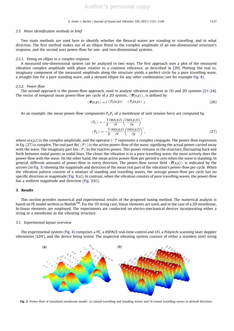
where u(x,y,t) is the complex amplitude, and the operator ( � )n represents a complex conjugate. The power-flow expressionin Eq. (27) is complex. The real part Re(/PS) is the active power-flow of the wave, signifying the actual power carried awaywith the wave. The imaginary part Im(/PS)is the reactive power. This power remains in the structure, fluctuating back andforth between nodal points or nodal lines. The closer the vibration is to a pure travelling wave, the more actively does thepower-flow with the wave. On the other hand, the mean active power-flow per period is zero when the wave is standing. Ingeneral, different amounts of power-flow in every direction. The power-flow vector field /P(x,y)S is indicated by thearrows (in Fig. 3) showing the magnitude and direction of the mean real part of the vibration’s power-flow per cycle. Whenthe vibration pattern consists of a mixture of standing and travelling waves, the average power-flow per cycle has nospecific direction or magnitude (Fig. 3(a)). In contrast, when the vibration consists of pure travelling waves, the power-flowhas a uniform magnitude and direction (Fig. 3(b)).

3. Results

This section provides numerical and experimental results of the proposed tuning method. The numerical analysis isbased on FE model written in MatlabTM. For the 1D string case, linear elements are used, and in the case of a 2D membrane,bi-linear elements are employed. The experiments are conducted on electro-mechanical devices incorporating either astring or a membrane as the vibrating structure.

3.1. Experimental layout overview

The experimental system (Fig. 4) comprises a PC, a dSPACE real-time control and I/O, a Polytech scanning laser dopplervibrometer (LDV), and the device being tested. The inspected vibrating system consists of either a stainless steel string

Fig. 3. Power-flow of simulated membrane model: (a) mixed travelling and standing waves and (b) tuned travelling waves in desired direction.



(Fig. 5) excited by two actuators, or a polyurethane membrane excited by 32 actuators (Fig. 6). The membrane is taut andconnected to the frame by circumferential springs. A MatlabTM program running on the PC commands the real-timedSPACE environment and a VXI data acquisition system (VXITech, VT1433B). The dSPACE system controls an externalpower amplifier containing current drivers. The amplitude and phase of the 32 voice-coil actuators are controlled by 32

Fig. 4. Experiment system layout.

Fig. 5. Experimental system consisting of a taut string and two exciters scanned by LDV.

Fig. 6. Membrane experimental system: (a) top view and (b) front view.



digital-to-analogue converters. The vibrating string and membrane structures are equipped with 73 and 1263 diffusivityenhancing stickers, respectively, that are measured by the LDV. The LDV output is filtered (LP Filter of 2.56 kHz), sampled(at 6.55 kHz), and recorded by the VXI sampling unit connected to the PC via firewire. The frequencies of interest are inorder of 101–102 Hz. The recorded digital data is sine-fitted according to the input frequencies and their harmonics, then itis further processed using a dedicated MatlabTM code implementing the described tuning method.

3.2. Numerical and experimental tuning results for one-dimensional string system

In this section, numerical and experimental results are presented for a taut string model and experimental device. Theseresults are used to validate the proposed tuning method for single and multi-frequency tuning, including wavelengthoptimization and model matrix analysis of 1D structures.

3.2.1. Single frequency tuning

The wavelength optimization described in Section 2.4 (Eqs. (20)–(22)) was verified by simulations on the FE stringmodel, with artificial noise added to the simulated measurements. The results can be seen in Fig. 7(a).

A definite global minimum is observed for the quality measure (mismatch function). Nevertheless, as might be expectedsome local minima are also present in the rational fractions of l0 (that might affect some minimum-seeking solvers).Similar behavior was found during the optimization routine applied to experimentally measured data from the stringdevice, as can be seen in Fig. 7(b).

After model identification and wavelength optimization were completed experimentally, the two actuators were tunedto generate several vibration patterns of standing wave and travelling wave at some distance from the string boundaries.A third combination representing an arbitrary mixture of standing and travelling waves was also measured for comparison.The measured complex response of the three cases was plotted on the complex plane, and the corresponding real andimaginary components of the mean power-flow are given in Fig. 8. As expected, the complex response of a standing wavetraces a straight line and the mean active power-flow approaches zero (Fig. 8(a) and (d)). In contrast, the complex responseof a travelling wave (Fig. 8(c) and (f)) approaches a circle, and the mean active power-flow approaches a nonzero uniformvalue, whose sign represents the direction of wave propagation. The imaginary component of the mean power-flowrepresents the reactive power, i.e. the power cycling within the string system. Note that for the standing and mixed-wavescases, the imaginary component oscillates along the string, while for the pure travelling wave this part approaches zero(Figs. 8(d)–(f), respectively).

3.2.2. Multi-frequency tuning

For the sake of improved interpretation of the measured results of a multi-frequency response, the dynamic complianceof the string was measured in the relevant frequency domain, and is given in Fig. 9. The curve shape corresponds with theobtained results, as discussed below.

Two multi-frequency tuning sets of measurements are presented here. Each set includes the simultaneous tuning ofthree harmonics. The string was first tuned at 33, 66, 99 Hz. At these frequencies, the structure’s response amplitude gain israther moderate (see Fig. 9), a finding addressed in analyzing the topology of the model matrix H. The string was tuned toincorporate three travelling waves simultaneously at the three harmonics 33, 66, 99 Hz of the same 0.1 mm amplitude.Fig. 10 shows the measured complex response after one and five perturbations. The final result yields three circles ofapproximately the same radius, indicating a response comprising three travelling waves with the same amplitude ofabout 0.1 mm.

Fig. 7. String: response mismatch vs. wavelength (Eq. (22)): (a) by simulation and (b) by measured data.



Yet when the string’s structure was measured and analyzed at the second frequency set 30, 60, 90 Hz, which is closer tonatural frequencies (see Fig. 9), a different model was identified. The string device was tuned for a travelling wave at 60 Hzonly. Undesired responses at 30 and 90 Hz were actively decayed. These parasitic harmonics were expected to arise due tocross-coupling in the response, as discussed in Section 3.2.4. The results after one and twelve perturbations are shown inFig. 11. The initial response in Fig. 11(a) shows a very thin ellipse in the first harmonic, indicating an undesired significantstanding wave at 30 Hz with an amplitude of about 1 mm. The final response shows a circle with a radius of approximately0.1 at 60 Hz with remaining small responses of about 0.02 at 30 and 90 Hz. This indicates a nearly pure travelling wave wascreated at 60 Hz at the desired amplitude of 0.1 mm with residual responses of about 0.02 mm at 30 and 90 Hz. Theseresults indicate that nonlinear adaptation via perturbation facilitates reduction of an unwanted dominant standing waveby two orders of magnitude.

Tuning at the frequency set 30, 60, 90 Hz required more perturbation steps than at 33, 66, 99 Hz to sufficiently approachthe desired response. Clearly, the high amplitudes gave rise to some nonlinear coupling between the various harmonics.

3.2.3. Real-time wave measurement—verification

The real-time velocities of two points along a string undergoing a single frequency excitation were measuredsimultaneously using two LDVs. The LDVs first measured the same point and then measured two points displaced a quarter

Fig. 8. (a) Complex measured response in (mm) of tuned standing wave: (b) mixed waves and (c) tuned travelling wave. Measured, fitted; (d) real

and imaginary power-flow in arbitrary units of standing waves, (e) mixed waves and (f) standing waves, real power-flow, - - imaginary power-flow.

Fig. 9. Measured typical dynamic compliance of the string.



of a wavelength apart. The two measured signals were connected to the x and y channels of an oscilloscope. Measuring thesame point should yield a straight line in the Lissajou diagram, while measuring two points separated by a quarterwavelength while assuming travelling waves with only one dominant harmony (linear system) should yield a perfectcircle. The two measurements at 100 Hz are depicted in Fig. 12(a) and (b), respectively. Real-time Lissajou plots provide anaccurate verification of the fact that a monochromatic travelling wave has been formed. The alternative approach that uses

Fig. 10. Measured complex response of tuned travelling waves at 33, 66, 99 Hz simultaneously: (a) after one iteration, and (b) after five iterations.

( ) Measured at 33 Hz, ( ) measured at 66 Hz, ( ) measured at 99 Hz, ( ) fitted at 33 Hz, (- -) fitted at 66 Hz and ( ) fitted at 99 Hz.

Fig. 11. Measured complex response of tuned travelling waves at 60 Hz while simultaneously decaying parasitic responses at 30 and 90 Hz: (a) after one

iteration, (b) after 12 iterations. ( ) Measured at 30 Hz, ( ) measured at 60 Hz, ( ) measured at 90 Hz, ( ) fitted at 30 Hz, (- -) fitted at 60 Hz, and

( ) fitted at 90 Hz.

Fig. 12. Lissajou diagram of two time-response signals measured at points along a string experiencing travelling wave: (a) at the same location and

(b) quarter wavelength apart.



the complex amplitude data measured along the structure uses an inevitable curve-fit stage where the average results canonly be displayed.

3.2.4. Model matrix H analysis—measured data

The single-frequency model matrix components defined in Eq. (5) were first examined for single frequency tuningunder moderate input amplitudes at 85 Hz, far from any of the structure’s natural frequencies (see Fig. 9). The result isdepicted in Fig. 13, where the x- and y-axis stand for the H matrix row and column indices, and the numerical value of eachelement is color coded. The four columns represent the cosine and sine terms of the two actuators, (2M¼ 4), and the rowsrepresent the cosine and sine terms of the 38 measured points (2N ¼ 76) along the string. The upper left and lower rightblocks in Fig. 13, separated by dashed lines, signify the structure’s cosine terms response to the cosine terms of the input,and the same applies for the sine terms, respectively (see Eqs. (3)–(5) and (8), (9)). The off-diagonal blocks are thestructure’s response in cosine terms to sine input terms, and vice versa.

The anticipated block structure as given in Eq. (9) is clearly observed, implying a certain level of linearity in thatparticular operation regime. The off-diagonal terms are clearly smaller in magnitude than the diagonal blocks, indicatinga negligible phase lag implying low damping and an excitation frequency far enough from any natural frequency.The diagonal blocks are nearly identical, and the off-diagonal terms have opposite signs, as predicted by Eq. (9).

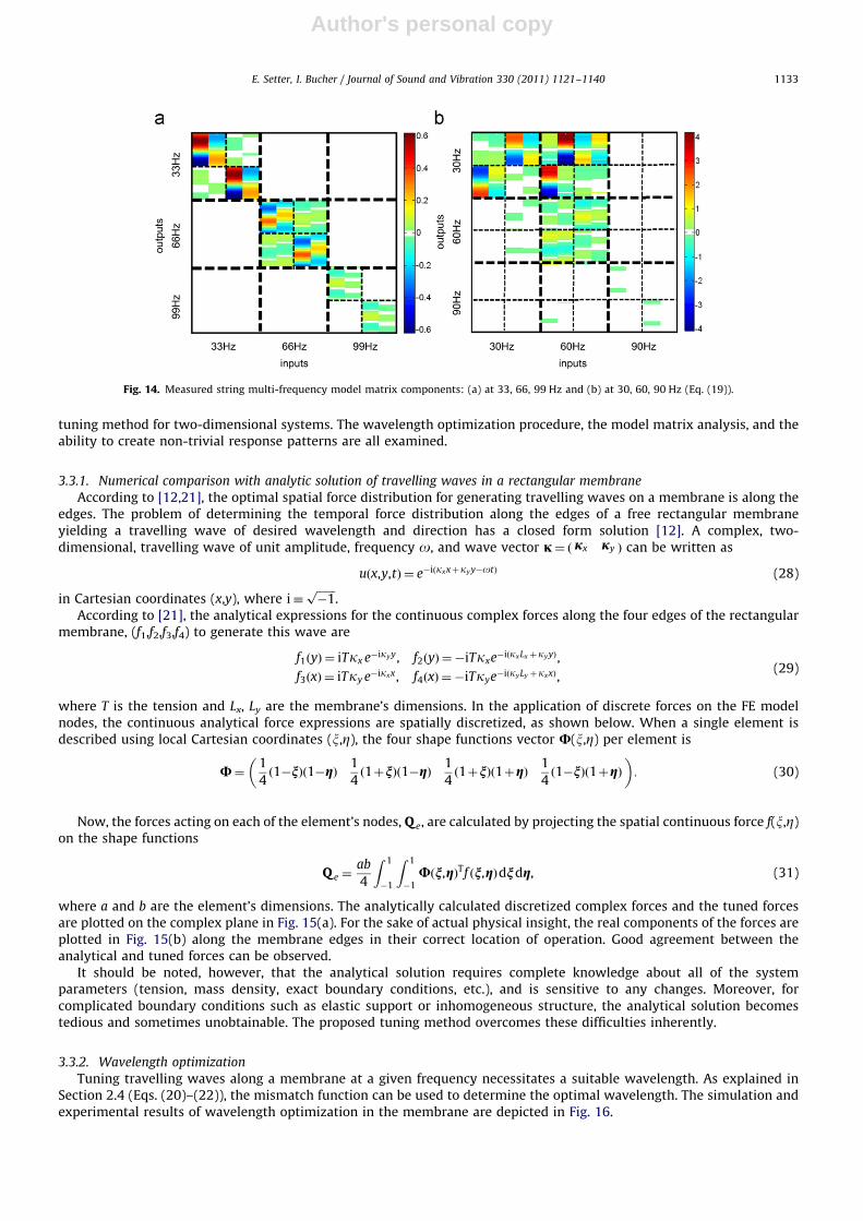
In accordance with Eq. (19), the multi-frequency matrix model was analyzed for the two sets of frequencies: 30, 60, 90and 33, 66, 99 Hz. The results are presented in Fig. 14. The components in Fig. 14 are divided into bigger and smaller blocksby wide and thin dashed lines, respectively. The wider dashed lines indicate the frequency blocks, and the thinner indicatecosine and sine terms as before. The larger diagonal blocks represent the response at a given frequency to excitation at thesame frequency, while the larger off-diagonal blocks represent the excitation of super- or sub-harmonics, i.e. frequencycross-coupling. The anticipated linear model can be seen in Fig. 14(a) for 33, 66, 99 Hz, where the large off-diagonal blocksapproach zero, indicating negligible cross-coupling. In Fig. 14(b), however, the string structure model for the frequency set30, 60, 90 Hz, i.e. closer to the natural frequencies, is different. The model differs both in its diagonal blocks and in itsoff-diagonal blocks. A strong asymmetric sub-harmonic response is observed at H1,2 (notation according to Eq. (19)),indicating a response at 30 Hz to excitation at 60 Hz. The upper left block of Fig. 14(b) represents H1,1, or the response at30 Hz to excitation at 30 Hz. An examination of the smaller blocks of H1,1 reveals more dominant off-diagonal components,indicating in-quadrature response, as expected for a structure excited close to one of its natural frequencies. The resultsshown here suggest that unsuccessful choice of excitation frequency can distort the obtained response considerably. Still,when the nature of these distortions, i.e. nonlinear behavior causing harmonics, is accounted for, their effect can beidentified and nullified.

3.3. Numerical and experimental tuning results of two-dimensional membrane system

This section presents the numerical and experimental results of tests carried out on a membrane using the proposedmethod. A closed form analytical solution is compared with the tuning method results for an ideal case to validate the

Fig. 13. Model matrix (H) components—measured string model at 85 Hz (Eq. (10)).



tuning method for two-dimensional systems. The wavelength optimization procedure, the model matrix analysis, and theability to create non-trivial response patterns are all examined.

3.3.1. Numerical comparison with analytic solution of travelling waves in a rectangular membrane

According to [12,21], the optimal spatial force distribution for generating travelling waves on a membrane is along theedges. The problem of determining the temporal force distribution along the edges of a free rectangular membraneyielding a travelling wave of desired wavelength and direction has a closed form solution [12]. A complex, two-dimensional, travelling wave of unit amplitude, frequency o, and wave vector j¼ ðjx jy Þ can be written as

uðx,y,tÞ ¼ e�iðkxxþkyy�otÞ (28)

in Cartesian coordinates (x,y), where i�ffiffiffiffiffiffiffi�1p

.According to [21], the analytical expressions for the continuous complex forces along the four edges of the rectangular

membrane, (f1,f2,f3,f4) to generate this wave are

f1ðyÞ ¼ iTkx e�ikyy, f2ðyÞ ¼�iTkxe�iðkxLxþkyyÞ,

f3ðxÞ ¼ iTky e�ikxx, f4ðxÞ ¼�iTkye�iðkyLy þkxxÞ,(29)

where T is the tension and Lx, Ly are the membrane’s dimensions. In the application of discrete forces on the FE modelnodes, the continuous analytical force expressions are spatially discretized, as shown below. When a single element isdescribed using local Cartesian coordinates (x,Z), the four shape functions vector U(x,Z) per element is

U¼1

4ð1�nÞð1�gÞ

1

4ð1þnÞð1�gÞ

1

4ð1þnÞð1þgÞ

1

4ð1�nÞð1þgÞ

� �: (30)

Now, the forces acting on each of the element’s nodes, Q e, are calculated by projecting the spatial continuous force f(x,Z)on the shape functions

Q e ¼ab

4

Z 1

�1

Z 1

�1Uðn,gÞTf ðn,gÞdndg, (31)

where a and b are the element’s dimensions. The analytically calculated discretized complex forces and the tuned forcesare plotted on the complex plane in Fig. 15(a). For the sake of actual physical insight, the real components of the forces areplotted in Fig. 15(b) along the membrane edges in their correct location of operation. Good agreement between theanalytical and tuned forces can be observed.

It should be noted, however, that the analytical solution requires complete knowledge about all of the systemparameters (tension, mass density, exact boundary conditions, etc.), and is sensitive to any changes. Moreover, forcomplicated boundary conditions such as elastic support or inhomogeneous structure, the analytical solution becomestedious and sometimes unobtainable. The proposed tuning method overcomes these difficulties inherently.

3.3.2. Wavelength optimization

Tuning travelling waves along a membrane at a given frequency necessitates a suitable wavelength. As explained inSection 2.4 (Eqs. (20)–(22)), the mismatch function can be used to determine the optimal wavelength. The simulation andexperimental results of wavelength optimization in the membrane are depicted in Fig. 16.

Fig. 14. Measured string multi-frequency model matrix components: (a) at 33, 66, 99 Hz and (b) at 30, 60, 90 Hz (Eq. (19)).



The wavelength optimization method does not require any information about the model’s geometry or the materialconstants. Based on pure experimentally obtained data, the offline optimization searches for the best wavelength favoredby the system under test conditions. As in the one-dimensional system (Fig. 7), a clear global minimum can be seen inFig. 16.

3.3.3. Model matrix H analysis—measured data

Eq. (10) was used to calculate a membrane’s single frequency model based on measured data incorporating theexcitation of 32 actuators ð2M¼ 64Þ and 589 measured points ð2N ¼ 1178Þ at an excitation frequency of 40 Hz. Accordingto the measured dynamic compliance of the membrane (given in Fig. 17) the membrane gain is moderate at the chosenexcitation frequency, so that linear behavior can be expected.

The linearity level was examined by inspecting the measured model block-matrix structure depicted in Fig. 18, as in thestring case (Fig. 13).

Clearly, the hyper block-matrix shown in Fig. 18 has the same topology as that of Eq. (9) and is thus an indication ofhigh linearity at the chosen operation regime.

3.3.4. Tuning single and multi-frequency travelling waves and vortexes

The tuning algorithm was tested numerically to generate a travelling wave with a given amplitude and wave vector j,as given in Eqs. (24) and (25). The membrane was modeled by FE scheme with uniform tension and concentrated massesand springs at each actuation node, in this case only along the boundaries. Simulated results along with the real meanpower-flow are shown in Fig. 2(b). The membrane experiment device (see Fig. 6) was used for the two-dimensional tuningexperiments. The surface of the membrane, at some distance from the boundaries, was tuned for travelling waves at

Fig. 15. Comparison between analytic and tuned forces: (a) complex and (b) real components. ( ) and ( ) tuned, ( ) analytic.

Fig. 16. Membrane response mismatch vs. wavelength (Eq. (22)): (a) by simulation and (b) by measured data at 40 Hz.



different directions by a number of actuators (here 6–10) located along the boundaries. The measured results depicted inFig. 19 show that a desired wave can be tuned by actuators residing far from the tuned area.

The location of the actuators can be visibly traced by noting the area with larger amplitudes, as depicted in Fig. 19(c)and (d). According to the calculated power-flow given by the arrows in Fig. 19, the tuned area shows the desired travellingwave response, while the peripheral area exhibits a periodic arbitrary vibration.

The tuning algorithm was next used numerically to simulate a 2D response incorporating several harmonics in the formof a truncated Fourier series shaped as a travelling triangular wave. The tuning algorithm should tune each harmonic toyield a travelling wave at a specific amplitude, and all the waves having different frequencies should travel in-phase and atthe same direction of propagation. The truncated Fourier series, consisting of P harmonics, describing such a response

Fig. 18. Model matrix (H) components—measured membrane model at 40 Hz (Eq. (10)).

Fig. 17. Measured typical dynamic compliance of the membrane.



can be written as

uðx,y,tÞ ¼8

p2

XPn ¼ 1

1

ð2n�1Þ2cos jnUr�ð2n�1Þx0tð Þ

¼8

p2

XPn ¼ 1

1

ð2n�1Þ2cosðjnUrÞcosðð2n�1Þx0tÞþsinðjnUrÞsinðð2n�1Þo0tÞð Þ, (32)

where o0 is the basic harmonic, jn is the nth wave vector, and r is the position vector as defined below Eq. (23).The simulated response with the power-flow analysis of a series of five harmonics is given in Fig. 20.

Other series such as a rectangular travelling wave or a half-sine pulse can be similarly approximated. Indeed, they werealso simulated successfully, though are not described here due to space limitations.

The proposed method was next used to tune rotating waves in a rectangular membrane at a variety of circularwavelengths and frequencies. To this end, the desired response was presented as a separable time–space function in termsof sine/cosine coefficients. The function can be written in polar coordinates as

uðr,y,tÞ ¼ sinðkrrÞcosðkyy�otÞ, (33)

where kr and ky are scalars dictating the spatial frequencies (wavenumbers) along the radius and along the circumference,respectively. To satisfy circular continuity, ky must be an integer. The temporal frequency of the excitation governing therotation speed is o. Transforming Eq. (33) into Cartesian coordinates and expanding yields

uðx,y,tÞ ¼ sin jr

ffiffiffiffiffiffiffiffiffiffiffiffiffiffiffix2þy2

q� �cosðjh arctanðy=xÞ�xtÞ

¼ sin jr

ffiffiffiffiffiffiffiffiffiffiffiffiffiffiffix2þy2

q� �cosðjh arctanðy=xÞÞcosxtþsinðjh arctanðy=xÞÞsinxt� �

: (34)

Fig. 19. Measured travelling wave along a membrane with the real mean power-flow at four different directions of advance: (a) mid membrane tuned

and measured, y=01, (b) mid membrane tuned and measured, y=451, (c) mid membrane tuned all membrane measured, y=901, (d) mid-membrane tuned

all membrane measured, y=1801 (excitation using 6–10 actuators at 40 Hz).

Fig. 20. Power-flow of triangular travelling wave of 5 harmonics (from 10 Hz)—FE model simulation.



As before, kr (and ky) are also determined by minimizing the two dimensional mismatch function Jmis(kr,ky) in order toestablish the optimal wavelength given a predetermined frequency, where

Jmisðjr ,jhÞ ¼:eðjr ,jhÞ::adðjr ,jhÞ:

, (35)

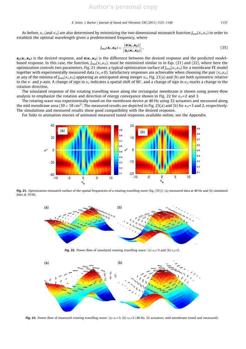
adðjr ,jhÞ is the desired response, and eðjr ,jhÞ is the difference between the desired response and the predicted model-based response. In this case, the function, Jmis(kr,ky), must be minimized similar to in Eqs. (21) and (22), where here theoptimization controls two parameters. Fig. 21 shows a typical optimization surface of Jmis(kr,ky) for a membrane FE modeltogether with experimentally measured data (kra0). Satisfactory responses are achievable when choosing the pair (kr,ky)at any of the minima of Jmis(kr,ky) appearing as anticipated along integer ky. Fig. 21(a) and (b) are both symmetric relativeto the x- and y-axis. A change of sign in kr indicates a spatial shift of 901, and a change of sign in ky marks a change in therotation direction.

The simulated response of the rotating travelling wave along the rectangular membrane is shown using power-flowanalysis to emphasize the rotation and direction of energy conveyance shown in Fig. 22 for ky=2 and 3.

The rotating wave was experimentally tuned on the membrane device at 40 Hz using 32 actuators and measured alongthe mid membrane area (30�18 cm2). The measured results are depicted in Fig. 23(a) and (b) for ky=3 and 2, respectively.The simulations and measured results show good compatibility with the desired response.

For links to animation movies of animated measured tuned responses available online, see the Appendix.

Fig. 21. Optimization mismatch surface of the spatial frequencies of a rotating travelling wave (Eq. (35))): (a) measured data at 40 Hz and (b) simulated

data at 10 Hz.

Fig. 22. Power-flow of simulated rotating travelling wave: (a) ky=3 and (b) ky=2.

Fig. 23. Power-flow of measured rotating travelling wave: (a) ky=3, (b) ky=2 (40 Hz, 32 actuators, mid-membrane tuned and measured).



4. Conclusions

The presented numerical and experimental results indicate that the proposed tuning method has several advantages overother vibration tuning methods. Analytical force distribution calculation, for example, is highly dependent upon systemparameters (tension, mass density, etc.), and is confined to simple geometries and boundary conditions. However, the proposedmethod requires little or even no previous knowledge of the system at hand prior to tuning. Moreover, dual- or multimodeexcitation, as a method to produce travelling waves, produces suboptimal results. These often combine vibration modes withslightly different wavelengths thus producing a standing wave component accompanying the travelling part. However, thepresented non-modal method automatically detects and excites the required modes of vibration comprising the desiredresponse, thus resulting in nearly pure travelling waves at the tuned area, however with somewhat lower amplitudes.

The proposed method is also capable of generating a desired response in the presence of nonlinear, undesired, sub- or super-harmonics. As shown, by dictating zero amplitude oscillation for unwanted frequencies, the algorithm drives energy into thesystem to actively decay these parasitic oscillations. Convergence by small perturbations allows the algorithm to achieve thedesired response in mild nonlinear vibration regimes, such as in the proximity of natural frequencies, where amplitudes tend torise. This capability is important in composing the response of a series incorporating several frequencies, as in the case of atriangular travelling wave, where all the terms should be in phase and the amplitudes ratios are predetermined.

The proposed tuning method was successfully applied to tuning vibration patterns that are not the well-known solutionof the wave equation. Rotating vortexes as well as translatory travelling waves were realized numerically andexperimentally on the same structure. The presented method automatically finds the combination of forces to yield theclosest response possible to the desired one.

This paper has presented new techniques for linearity assessment. The analysis is based on comparing the structure ofthe measured system model matrix with the theoretical linear block structure (Eq. (9)). Nonlinear effects such as sub- orsuper-harmonics are detected by the cross-coupling blocks of the multi-frequency model (Eq. (19)).

This paper has proposed wavelength optimization methods that minimize the anticipated mismatch between thedesired responses for one- and two-dimensional structures. These methods are used to optimize the measured response.

Movie 1. Animated measurements of a travelling wave propagating at an angle y=01. Tuning and measuring are conducted on the same 30�18 cm2

membrane section.

Movie 2. Animated measurements of a travelling wave propagating at an angle y=01 on a 46�26 cm2 membrane section. Tuning was conducted on the

mid 30�18 cm2 section.



Acknowledgements

This work has been partially supported by the Israeli Science Foundation, Grant no. 574/04.The authors would like to acknowledge the contributions of Dr. Ran Gabai, Mr. Harel Plat, and Mr. Hadar Raz for sharing

their knowledge and enthusiasm with us.

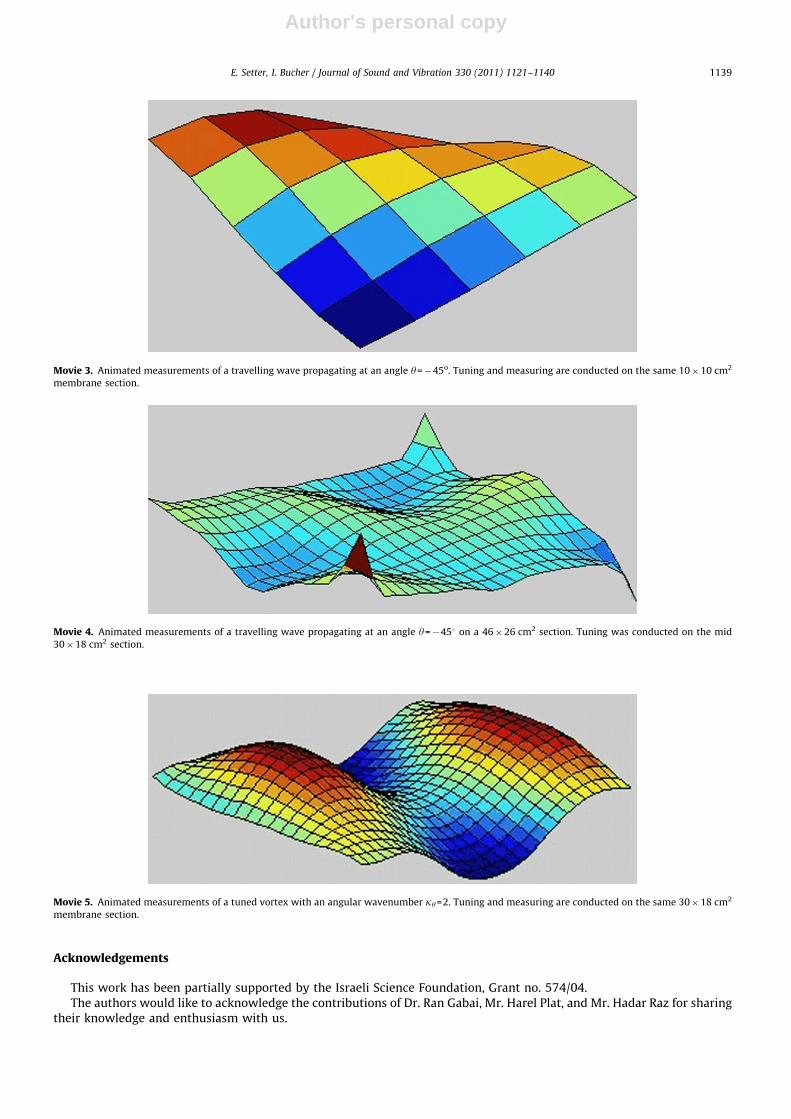
Movie 3. Animated measurements of a travelling wave propagating at an angle y=�45o. Tuning and measuring are conducted on the same 10�10 cm2

membrane section.

Movie 4. Animated measurements of a travelling wave propagating at an angle y=�451 on a 46�26 cm2 section. Tuning was conducted on the mid

30�18 cm2 section.

Movie 5. Animated measurements of a tuned vortex with an angular wavenumber ky=2. Tuning and measuring are conducted on the same 30�18 cm2

membrane section.



Appendix: Links to animations of experimental measurements

The following are the supplementary data to this article:Movies 1 to 6.

References

[1] A. Minikes, I. Bucher, Non-contacting lateral transportation using gas squeeze film generated by flexural travelling waves-numerical analysis, Journalof the Acoustical Society of America 113 (2003) 2464–2473.

[2] A. Minikes, R. Gabay, I. Bucher, M. Feldman, On the sensing and tuning of progressive structural vibration waves, IEEE Transactions on Ultrasonics,Ferroelectrics, and Frequency Control 52 (9) (2005) 1565–1575.

[3] Y. Chen, S. Ma, B. Li Wang, Analysis of travelling wave locomotion of snake robot, Proceedings of the 2003 IEEE, International Conference on Robotics,Intelligent Systems, and Signal Processing, Changsha, China, October 2003.

[4] L.E. Becker, S.A. Koehler, H.A. Stone, On self-propulsion of micro-machines at low Reynolds number: Purcell’s three-link swimmer, Journal of FluidMechanics 490 (2003) 15–35.

[5] W.J. O’Connor, D. Lang, Position control of flexible robot arms using mechanical waves, ASME Journal of Dynamics Systems, Measurement and Control120 (3) (1998) 334–339.

[6] H. Iwamoto, N. Tanaka, Adaptive feed-forward control of flexural waves propagating in a beam using smart sensors, Smart Materials and Structures 14(6) (2005) 1369–1376.

[7] H. Iwamoto, N. Tanaka, Feedforward control of flexural waves propagating in a rectangular panel, Journal of Sound and Vibration 324 (1-2) (2009)1–25.

[8] M. Kuribayashi, S. Ueha, E. Mori, Excitation conditions of flexural travelling waves for a reversible ultrasonic linear motor, Journal of the AcousticalSociety of America 77 (1985) 1431–1435.

[9] S. Ueha, Y. Tomikawa, with contributions from M. Kurosawa and N. Nakamura, Ultrasonic Motors: Theory and Applications, Clarendon Press, Oxford,1993.

[10] J.F. Manceau, S. Biwersi, F. Bastin, On the generation and identification of travelling waves in non-circular structures—application to innovativepiezoelectric motors, Smart Material Structures 7 (1997) 337–344.

[11] J.F. Manceau, F. Bastin, Production of quasi-travelling wave in a silicon rectangular plate using single phase drive, Transactions on Ultrasonic,Ferroelectric, and Frequency Control 42 (1) (1995).

[12] R. Gabai, I. Bucher, Spatial and temporal excitation to generate travelling waves in structures, Journal of Applied Mechanics 77 (2) (2010) 021010.[13] T.H. Vose, P. Umbanhowar, K.M. Lynch, Friction-induced velocity fields for point parts sliding on a rigid oscillated plate, International Journal of

Robotics Research 28 (8) (2009) 1020–1039.[14] C. Fink, S. Ergu’n, D. Kralisch, U. Remmers, J. Weil, T. Eschenhagen, Chronic stretch of engineered heart tissue induces hypertrophy and functional

improvement, The FASEB Journal 14 (2000) 669–679.[15] N. Tanaka, S.D. Snyder, Y. Kikushima, M. Kuroda, Vortex structural power flow in a thin plate and the influence on the acoustic field, Journal of the

Acoustical Society of America 96 (3) (1994) 1563–1574.[16] I. Bucher, Exact adjustment of dynamic forces in presence of non linear feedback and singularity—theory and algorithms, Journal of Sound and

Vibration 218 (1) (1998) 1–27.[17] G. Strang, K. Borre, Linear Algebra, Geodesy and GPS, Wellesley-Cambridge Press, MA, USA, 1997.[18] A. Ben-Israel, Thomas N.E. Greville, Generalized Inverses: Theory and Applications, Springer, New York, 2003.[19] B. Noble, J.W. Daniel, Applied Linear Algebra, 3rd ed., Prentice-Hall International, Englewood Cliffs, NJ, 1988.[20] I. Bucher, Estimating the ratio between travelling and standing vibration waves under non-stationary conditions, Journal of Sound and Vibration 270

(2004) 341–349.[21] R. Gabai, Generating, Sensing and Controlling Progressive Waves in One and Two Dimensions, a Theoretical and Experimental Study, PhD Thesis,

Technion-Isreali Institute of Technology, 2009.[22] J.D. Achenbach, Wave Propagation in Elastic Solids, NHPC (1973).[23] R. Gabai, E. Setter, H. Plat, I. Bucher, Power flow control and travelling waves of vibration, the optimal force distribution, ICEDyn International

Conference on Structural Engineering Dynamics, June 2009, Ericeria, Portugal.[24] M.J. Brennan, S.J. Elliott, R.J. Pinnington, Active control of flexural waves using power as a controlling parameter, Proceedings of the Fifth International

Conference on Recent Advances in Structural Dynamics, Southampton, UK, 2, 1994, pp. 973–982.

Movie 6. Animated measurements of a vortex with an angular wavenumber ky=3. Tuning and measuring are conducted on the same 30�18 cm2

membrane section.


author's personal copy - technion

Documents