australian fuel classification: stage ii
TRANSCRIPT
CLIMATE ADAPTATION FLAGSHIP
Australian Fuel Classification: Stage II National Burning Project
sub‐project no. 5
Jim Gould and Miguel Cruz
Report number: EP126505 31 August 2012

2
Enquiries should be addressed to:
Gary Featherston Australasian Fire and Emergency Service Authorities Council (AFAC) Level 5, 340 Albert Street, East Melbourne, Victoria 3002 Phone: +61 3 9419 2388
This material was produced with funding provided by the Attorney‐General’s Department through the National Emergency Management Program. The Australasian Fire and Emergency Service Authorities Council, Attorney‐General’s Department and the Australian Government make no representations about the suitability of the information contained in this document or any material related to this document for any purpose. The document is provided ‘as is’ without warranty of any kind to the extent permitted by law. The Australasian Fire and Emergency Service Authorities Council, Attorney‐General’s Department and the Australian Government hereby disclaim all warranties and conditions with regard to this information, including all implied warranties and conditions of merchantability, fitness for particular purpose, title and non‐infringement. In no event shall Australasian Fire and Emergency Service Authorities Council, Attorney‐General’s Department or the Australian Government be liable for any special, indirect or consequential damages or any damages whatsoever resulting from the loss of use, data or profits, whether in an action of contract, negligence or other tortious action, arising out of or in connection with the use of information available in this document. The document or material related to this document could include technical inaccuracies or typographical errors.
Citation
Gould J, Cruz M (2012) Australian Fuel Classification: Stage II. Ecosystem Sciences and Climate Adaption Flagship, CSIRO, Canberra Australia.
Copyright and disclaimer
© 2012 CSIRO
To the extent permitted by law, all rights are reserved and no part of this publication covered by copyright may be reproduced or copied in any form or by any means except with the written permission of CSIRO.
Important disclaimer
CSIRO advises that the information contained in this publication comprises general statements based on scientific research. The reader is advised and needs to be aware that such information may be incomplete or unable to be used in any specific situation. No reliance or actions must therefore be made on that information without seeking prior expert professional, scientific and technical advice. To the extent permitted by law, CSIRO (including its employees and consultants) excludes all liability to any person for any consequences, including but not limited to all losses, damages, costs, expenses and any other compensation, arising directly or indirectly from using this publication (in part or in whole) and any information or material contained in it.
Front cover photographs:
(anticlockwise from left): prescribed fire through fuels in the Tallarook State Forest (VIC), wildfires at Coulomb Point (WA) and Millstream National Park (WA) (source: Jennifer Hollis).

i
Contents
Acknowledgments ............................................................................................................................................. iii
Executive summary ........................................................................................................................................... iv
1 Introduction .......................................................................................................................................... 1
2 Australian Fuel Classification ................................................................................................................ 2
2.1 Objectives and scope .................................................................................................................. 2
2.2 Constraints to adoption .............................................................................................................. 7
3 Glossary of terms for bushfire fuels ...................................................................................................... 8
4 Guidelines for fuel assessment ............................................................................................................. 9
4.1 Sampling designs ....................................................................................................................... 10
4.2 Plot size ..................................................................................................................................... 12
4.3 Size of sample ........................................................................................................................... 13
4.4 Destructive fuel sampling ......................................................................................................... 17
4.5 Non‐destructive sampling ......................................................................................................... 18
4.6 Fuel dynamic models ................................................................................................................ 26
4.7 Remote sensing ......................................................................................................................... 32
4.8 Sampling procedures for fuel inventory ................................................................................... 38
5 References ........................................................................................................................................... 46
6 Appendix A: Glossary of terms ............................................................................................................ 55
7 Appendix B: Current practices of fuel assessment in forest and grassland fuels ............................... 96
ii
Figures Figure 2‐1. Framework of the core module for an Australian Fuel Classification (AFC) consisting of two essential components (1) fuel type and structural form, and (2) fuel parameters and attributes (Hollis et al. 2011) .............................................................................................................................................................. 5
Figure 2‐2. Proposed conceptual structure for the Australia Fuel Classification (AFC), the dash box indicates the framework of the core module of Australian Fuel Classification in Figure 2‐1 ............................ 6
Figure 4‐1. An example of a photoload sequence for the 1‐hr fuel component ............................................. 20
Figure 4‐2. Example of the fuel and fire behaviour guide for pruned radiata pine plantation 4–8 years old . 21
Figure 4‐3. Example of the fuel and fire behaviour guide for mid‐rotation (4–6 years) blue gum plantation ......................................................................................................................................................... 22
Figure 4‐4. Examples of fuel accumulation curves illustrating patterns of litter accumulation following fires in a range of vegetation types in Australia. .............................................................................................. 27
Figure 4‐5. Fuel accumulation curves for northeast Tasmania dry eucalypt forest. Accumulation cures (solid line), 95% confidence bands for the accumulation curves (dotted red lines) and prediction bans for new sites (dotted black lines) ........................................................................................................................... 29
Figure 4‐6. Change in (a) surface, (b) near‐surface fuel, (c) elevated fuel and (d) overstorey tree bark hazard score in areas of different age fuel after burning at low and tall shrub sites ...................................... 31
Figure 4‐7. Proposed set of process for characterising wildland‐urban interface (WUI) fuels with the potential application of LiDAR imagery for assessment ................................................................................... 36
Figure 4‐8. Maps depicting (a) a hillshade model of gridded LiDAR data and (b) the planar extent of trees and buildings form the LiDAR data ................................................................................................................... 36
Tables Table 2‐1. Fuel classification applications across different spatial scales ......................................................... 7
Table 4‐1. Plot sizes used in bushfire fuel sampling in selected fuel types ...................................................... 15
Table 4‐2. Examples of fuel accumulation summary of parameters describing patterns of litter accumulation following fires in a range of vegetation types in Australia ........................................................ 28
Table 4‐3. Advantages, disadvantages, techniques and scales of different remote sensing data applied to fuel mapping ..................................................................................................................................................... 33
Table 4‐4. Sampling procedures for different fuel parameters by fuel type ................................................... 40
Table 4‐5. Suitability of sampling technique bases on the accuracy and cost of estimating different fuel parameters and/or attributes .......................................................................................................................... 44
iii
Acknowledgments
We thank the Australasian Fire and Emergency Service Authorities Council and Forest Fire Management
Group and value the opportunity to provide a report on Stage II of the Australian Bushfire Fuel
Classification.
This project was made possible through funding from the Attorney General’s Department as part of the
National Emergency Management Projects NEMP 1112‐00043, Australian Bushfire Fuel Classification
System.
Information on current practice in Australia and fuel classification requirements has arisen from comments and feedback given by practitioners and researchers within the AFAC Project Working Group and at two National Bushfire Fuel Classification workshops held in Melbourne in April 2011 and 2012. We value the contributions of practitioner and researcher participants in this workshop.
iv
Executive summary
1. Scope and objective
a. Fuel classification is key to effective fire management because it provides a simple way to
input extensive fuel characteristics into fire behaviour models, and supports a variety of
land and fire management activities.
b. The main objectives of the fuel classification are:
(i) to synthesise and catalogue fuel attributes required by fire behaviour models and
other land management tools (e.g. smoke production, carbon release) into a finite
set of classes or categories that ideally represent all possible fuel beds or fuel types
in a region and their subsequent fire behaviour and effects
(ii) to catalogue fuel attributes and parameters describing the dynamics and physical
structure of each fuel type
(iii) to maintain a fuel library (containing concepts, definitions, and references) and
documentation of procedures and guidelines for assessment and inventory of fuels.
c. Fuel classification will provide a standard framework for organising fuel descriptions that
provide an interface between the complexities of bushfire fuels data and the requirements
of the users of fire behaviour models, fuel hazard assessment, prescribed burning, risk
management, etc.
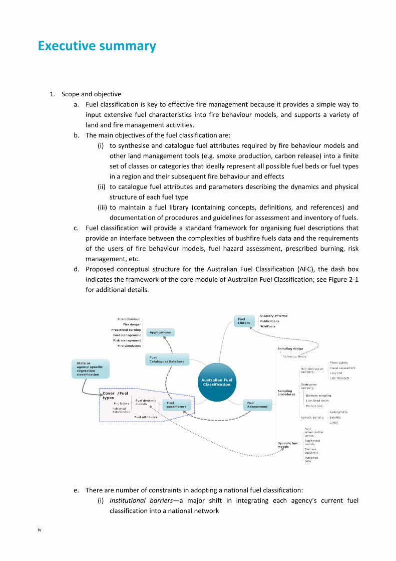
d. Proposed conceptual structure for the Australian Fuel Classification (AFC), the dash box
indicates the framework of the core module of Australian Fuel Classification; see Figure 2‐1
for additional details.
e. There are number of constraints in adopting a national fuel classification:
(i) Institutional barriers—a major shift in integrating each agency’s current fuel
classification into a national network

v
(ii) Documentation and training material availability—documentation and training
material is required to implement the fuel classification program
(iii) Current knowledge gaps and fuel sampling needs—e.g. fuel data is lacking for a
number of fuel types throughout Australia
(iv) Custodian role—the need for an organisation to assume a custodian role to update
and maintain a national fuel classification.
2. Glossary of terms
a. Imprecise use of certain terms regarding bushfire fuels often cause confusion and
misunderstanding, thus a glossary of terms, presented in Appendix A, gives definitions of
most commonly used terms.
b. Key terms of reference for this report are:
i. Fuels—are defined in terms of physical characteristics of live and dead biomass,
which contribute to the spread, intensity and severity of bushfires
ii. Fuel type—can be defined as ‘an identifiable association of fuel elements of
distinctive species, form, size, arrangement, and continuity that will exhibit
characteristic fire behaviour under defined burning conditions’ (Merrill and
Alexander 1987, p 24)
iii. Fuel classification—synthesises fuel attributes required by fire behaviour models
and other wildland fire decisions into a finite set of classes or categories that ideally
represent all possible fuel beds or fuel types for a region and their subsequent fire
behaviour and effects.
c. Bushfire fuel terms are constantly evolving. Thus, the glossary presented here is not
exhaustive and needs to be reviewed for amendments and further updates of terms. To
handle these updates and provide inputs for new terms, a wiki model (i.e. WikiFuel) is
proposed, which will allow the fire community to contribute information to an evolving
encyclopaedia of concepts relating to fuel, including definitions of terms and the
methodologies used for describing fuels.
3. Fuel assessment
a. It is impractical to measure all fuel attributes to determine the fuel characteristics,
structure, continuity and quantity because the costs, in terms of time and money, are
deemed too expensive when compared to the value placed on the usefulness of the
information obtained.
b. It is difficult to sample fuel for a variety of reasons:
i. Fuel descriptions include a diverse set of component that are often differentiated
by the objectives of the fuel sampling project.
ii. A single technique or method can be impractical or ineffective because of the size,
frequency and position of the fuel components.
iii. There are numerous designs and procedures for sampling of fuel characteristics for
a range of bushfire management decision support systems, which can be confusing
to fire managers when selecting a design.
c. Procedures and worked examples are given ranging from simple and rapid visual
assessment to highly detailed measurements of complex fuel structure along transects or
quadrants, which take considerable time and effort.
d. Sampling techniques discussed here provide different measures of fuel attributes, i.e. fuel
load estimated by destructive sampling versus visual assessment or fuel dynamic models,

vi
grass curing assessment by line transect versus remote sensing. Choosing one technique
that may not include sampling other fuel attributes involves tradeoffs between accuracy,
time, money, training, scale and effectiveness.
e. Fire and land management agencies commonly use the Overall Fuel Hazard Rating for fuel
assessment in dry eucalypt forest because the technique is rapid, as well as easily taught
and implemented. Although the visual hazard assessment is subjective, hazard ratings can
be related to difficulty of suppression, and fire behaviour (either fuel hazard rating or
numeric fuel hazard score).
f. The hazard rating represents a surrogate of fuel attributes of fuel structure, arrangement,
continuity, and live–to‐dead ratio and pattern of dynamics over time. There is limited
evidence to support the relationship between fuel hazard rating and fuel load and vice
versa. Recent research showed the Overall Fuel Hazard Rating fuel load tables to be a poor
indicator of fuel loads in New South Wales forests.
g. Aerial photography and remote sensing can play an important role in fuel classification.
Continued review and research into the application of remote sensing for bushfire fuel
classification focusing on integration of mapping techniques, sensor data, and field
validation should be considered. In addition, ecosystem simulation modelling can play an
important role in quantifying gradients responsible for fuel distributions to aid in image
classification for bushfire fuel mapping.
h. A table containing sampling procedures (see Table 4.4) for fuel inventory has been
compiled to aid systematic field observation, sampling and recording of fuels. We
recommend that all land and fire management agencies use this table to establish a
national network of fuel classification for Australia.
1
1 Introduction
Land management and rural fire agencies, as part of the Australasian Fire and Emergency Service Authorities Council (AFAC) and Forest Fire Management Group (FFMG), have recognised the need for a national framework for the application of prescribed burning. This framework is to be based on the most recent scientific evidence, and will provide an agreed methodology for the recognition of risks in balance with objectives. To address these national needs, AFAC and FFMG have embarked on a National Burning Project supported by the Commonwealth Government National Emergency Management Project. The National Burning Project (NBP) comprises four key objectives:
review the best practices for prescribed burning with supporting knowledge and tools
develop a national risk analysis and monitoring framework for bushfire hazards, burn management risks, ecological risks and smoke hazards that includes a measurement and review program
develop training competencies and support material for prescribed burning
investigate the potential and design for a national bushfire fuel classification system
A number of sub‐projects are being undertaken to achieve these objectives. National Burning Project sub‐project no. 5: Australian bushfire fuel classification was commissioned by AFAC to further investigate and recommend the implementation of a suitable national bushfire fuel classification system or systems, which meets the practitioners’ needs and is supported by best practice guidelines and science. Hollis et al. (2011) recommended an Australian fuel classification to enable the categorisation and organisation fuel characteristics in order to capture spatial diversity as well as dynamic and structural complexity in a way that accommodates existing models for fire behaviour and assists development of the next‐generation fire prediction tools. The aim of this report is to identify the elements of the design for an Australian fuel classification and report to AFAC and FFMG on:
1. the objectives and scope for the Australian Fuel Classification (AFC)
2. a glossary of terms for bushfire fuels
3. a standard procedure for assessment and inventory of bushfire fuels
4. dissemination of the project to achieve a collaborative progress to implementation of the
AFC.
2
2 Australian Fuel Classification
2.1 Objectives and scope
Bushfire is a keystone event in much of the Australian landscape. Human impacts on the landscape have altered fuels within the Australian bush—forest, shrubland and grasslands. Primary production, land clearing, urban development of bushland, invasive species, and changes in land use policies have all combined to significantly change the type, size and arrangement of fuels. The accumulation of natural and altered fuels has often resulted in ecologically and socially unacceptable fire behaviour. Thus, public concern over the possibility of severe bushfires has increased dramatically in recent years. Fear of losing life and property to bushfires is especially pronounced in wildland–urban interface (WUI)—an area where homes and other human development intermix with bush and rural vegetation. It is paramount that communities and fire authorities in bushfire prone regions of Australia understand fire‐related characteristics of nearby bush (forest, grassland, shrublands, and other vegetation types), in order to comprehend the potential hazard of fuels and their related fire behaviour for more effective decision‐making.
Fuel classification is an essential component of fire management systems. It allows for the grouping of similar vegetation classes or fuel types based on fuel structural characteristics that are significant for fire behaviour and fire management. A fuel classification can be implemented at different spatial resolutions:
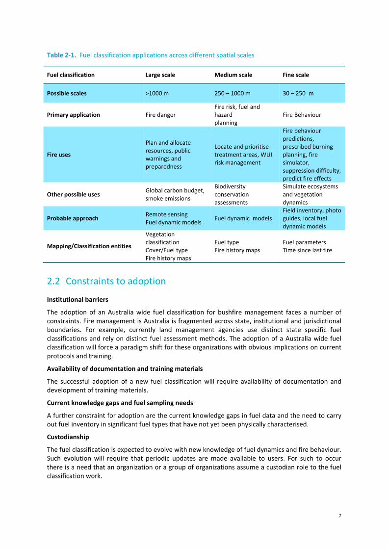
Coarse‐resolution classifications are useful in national‐ and state‐level fire danger
assessment, providing fire managers with information necessary to effectively plan, allocate
and mobilise suppression resources, issue public warnings, and meet legislative
requirements for bushfire policies and planning.
Medium‐resolution at a regional scale is useful for describing fire hazards to support
prioritisation of suppression resources, smoke management, strategic risk monitoring and
treatment and regional fire management planning and training.
Intermediate‐ and fine‐resolution of fuel classification attributes are necessary to predict site
specific fire behaviour and support fire suppression decision‐making, to identify and
evaluate tactically implemented fuel treatments, computing fire hazard and risk (the
potential damage and likelihood of that damage, respectively), and aiding in environmental
assessment.
In the development of fuel classification for bushfire management in Australia, Hollis et al. (2011) recommended that a fuel classification should:
1. be underpinned by a common, consistent, defined fuel terminology together with
standardised procedures for the assessment and inventory of fuel characteristics
2. contribute to improved understanding of fuel and fire behaviour
3. be of direct benefit to fire behaviour analysis and prediction
4. be peer reviewed
5. be flexible and adaptable over time
6. be capable of linking directly to geospatial vegetation databases and be in a format that can
potentially be integrated into an Australia‐wide spatial mapping tool.
3
A fuel complex is an association of fuel components based on vegetation communities (Pyne et al. (1996). Due to their complexity and role in bushfires, surface fuels (i.e. litter fuel) have received most research emphasis (McArthur 1962, 1967; Peet 1965; Sneeuwjagt and Peet 1985). Typically, a bushfire ignites in the surface fuel layer of the fuel complex. The surface fire intensity is the most important indicator of the likelihood that crown fire will ignite, and the limit of suppression capability. Cheney (1990) and Gould et al. (2007a, 2011) adopted a conceptual model whereby fire spread by burning across the top of a fuel bed and then down into the fuel bed. The model is subdivided into fuels that:
contribute to the flame height: primarily loosely compacted layers of surface, near‐surface
and elevated fuel
contribute to the depth of flame behind the fire front: the upper layer of the surface fuel
bed and the larger twig components imbedded in it
contribute to smouldering combustion: the lower compacted layers of the surface fuel, and
coarse woody material
burn only when supported by the combustion of lower fuels; these are generally sparse
elevated dead fuels, green fuels and some dead fuels >1 cm in diameter
do not burn because of their location, moisture content or size.
Fuels in eucalypt forests are not homogenous. They can be stratified into relatively compacted horizontal surface fuel layers with aerated, less‐compacted layers above; in some fuel types, the strata are quite distinct, e.g. overstorey trees, shrubs and grasses over litter. While small discontinuities in the surface litter layer (e.g. a narrow fire trail) can stop a low‐intensity fire, a high‐intensity fire may sweep across the same discontinuity, seemingly without impediment (Gould et al., 2011). There is strong evidence that the characteristics of the near‐surface fuel layer including continuity, bulk density, and fraction of green (live) material have a significant influence on fire spread (Cheney et al. 1992; Gould et al. 2007a, 2011; McCaw et al. 2012).
The different strata of a fuel complex were broken into fuel layers that can be directly related to fire spread or assessment of suppression difficulties (DEH 2006; DENR 2011a; Hines et al. 2010; Gould et al. 2007a, 2007b, 2011; McCarthy et al. 1999; Tolhurst et al. 1996; Wilson 1992, 1993). The fuel layers are:
overstorey tree bark and canopy
intermediate tree bark and canopy
elevated fuel
near‐surface fuel
surface fuel.
Fuel classification is key to effective fire management because it provides a simple way to input extensive fuel characteristics into fire behaviour models and supports various land and fire management needs (Hollis et al. 2011; Cruz and Gould 2009). The main objectives of the fuel classification are:
to synthesise and catalogue fuel attributes required by fire behaviour models and other
land management needs (e.g. fuel treatment, risk assessments, prescribe burning,
smoke management) into a finite set of classes or categories that ideally represent all
possible fuel beds or fuel types for a region and their subsequent fire behaviour and
effects
to catalogue fuel attributes and parameters describing the dynamics and physical
4
structure of each fuel type
to maintain a fuel library (containing concepts, definitions, and references) and
documentation of procedures and guidelines for assessment and inventory of fuels.
In facilitating the objectives and scope for an Australian Fuel Classification at the stakeholder workshop participants, representing land and rural fire management organizations across Australia, endorsed the fuel classification framework (Figure 2‐1) proposed by Hollis et al. (2011). At this workshop participants recommended that an Australian Fuel Classification should:
be underpinned by a common, consistent, defined fuel terminology together with
standardised procedures for the assessment and inventory of fuel characteristics
be flexible over time, adapting with advances in fuel and fire behaviour knowledge and
agreed changes to objectives
account for the dynamic nature of fuel characteristics
enable comparison across and within fuel types and change agents;
be able to be linked to a system to predict fire behaviour, existing and next‐generation fire
simulation models and fire management risk and decision systems
enable the generation of fuel maps across multiple scales.
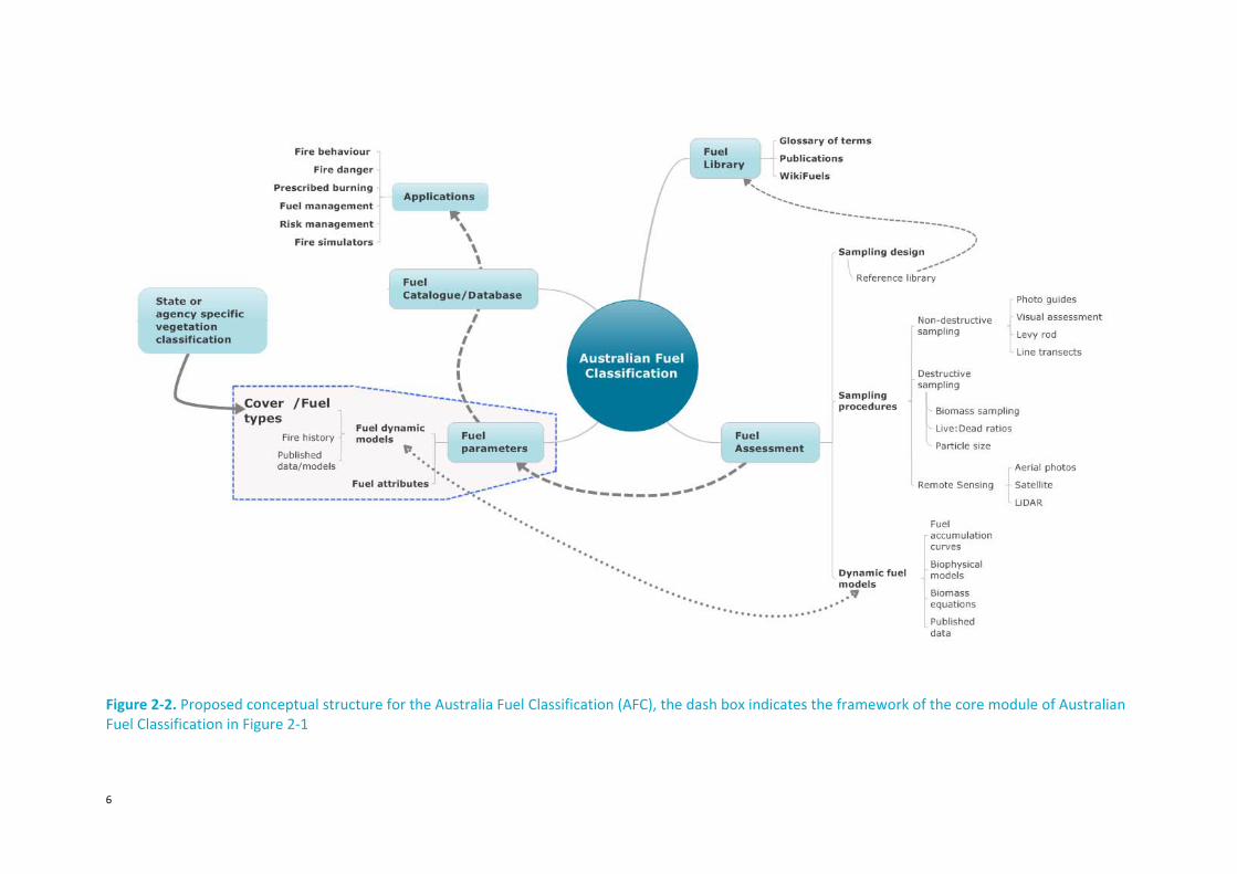
Figure 2‐2 is a conceptual structure for the proposed Australian Fuel Classification architecture. This structure has a wiki1 component (WikiFuels) to allow the fire community to contribute information to an evolving encyclopaedia of concepts relating to fuel, including definitions of terms and the methodologies used for describing fuels. The fuel classification should provide a standard framework for organising fuel descriptions that provides an interface between the complexities of bushfire fuel data and the requirements of the users of fire behaviour models, fuel hazard assessment, prescribed burning, risk management (described in Table 2‐1).
1 A wiki is a website whose users can add, modify, or delete its content via a web browser using a simplified mark up language or a rich‐text editor (see http://en.wikipedia.org/wiki/Wiki).
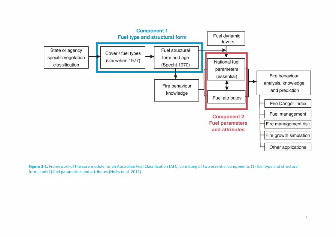
5
Figure 2‐1. Framework of the core module for an Australian Fuel Classification (AFC) consisting of two essential components (1) fuel type and structural form, and (2) fuel parameters and attributes (Hollis et al. 2011)
6
Figure 2‐2. Proposed conceptual structure for the Australia Fuel Classification (AFC), the dash box indicates the framework of the core module of Australian Fuel Classification in Figure 2‐1
7
Table 2‐1. Fuel classification applications across different spatial scales
Fuel classification Large scale Medium scale Fine scale
Possible scales >1000 m 250 – 1000 m 30 – 250 m
Primary application Fire danger Fire risk, fuel and hazard planning
Fire Behaviour
Fire uses
Plan and allocate resources, public warnings and preparedness
Locate and prioritise treatment areas, WUI risk management
Fire behaviour predictions, prescribed burning planning, fire simulator, suppression difficulty, predict fire effects
Other possible uses Global carbon budget, smoke emissions
Biodiversity conservation assessments
Simulate ecosystems and vegetation dynamics
Probable approach Remote sensing Fuel dynamic models
Fuel dynamic models Field inventory, photo guides, local fuel dynamic models
Mapping/Classification entities
Vegetation classification Cover/Fuel type Fire history maps
Fuel type Fire history maps
Fuel parameters Time since last fire
2.2 Constraints to adoption
Institutional barriers
The adoption of an Australia wide fuel classification for bushfire management faces a number of constraints. Fire management is Australia is fragmented across state, institutional and jurisdictional boundaries. For example, currently land management agencies use distinct state specific fuel classifications and rely on distinct fuel assessment methods. The adoption of a Australia wide fuel classification will force a paradigm shift for these organizations with obvious implications on current protocols and training.
Availability of documentation and training materials
The successful adoption of a new fuel classification will require availability of documentation and development of training materials.
Current knowledge gaps and fuel sampling needs
A further constraint for adoption are the current knowledge gaps in fuel data and the need to carry out fuel inventory in significant fuel types that have not yet been physically characterised.
Custodianship
The fuel classification is expected to evolve with new knowledge of fuel dynamics and fire behaviour. Such evolution will require that periodic updates are made available to users. For such to occur there is a need that an organization or a group of organizations assume a custodian role to the fuel classification work.
8
3 Glossary of terms for bushfire fuels
The previous project identified a lack of consistent terminology across agencies. Imprecise use of certain terms regarding bushfire fuels often causes confusion and misunderstanding. The glossary in Appendix A gives definitions of terms most commonly used in bushfire/wildland fire related to fuels. It includes terms that are commonly listed in wildland fire management glossaries (e.g. AFAC 2012; Merrill and Alexander 1987; NWCG 2011), and wildland fire management literature. This glossary provides an extensive listing of terms related to bushfire fuels, fuel assessment and definitions of fuel attributes used in fire behaviour prediction, fuel modelling and fuel hazard and risk assessment. The purpose of the glossary is to provide and maintain definition consistency and clarity for fuel terms for the Australian bushfire fuel classification. Each term is identified by one of three key categories:
1. General (G)—general reference terms for a fuel classification
2. Fuel (F) —detailed definition and descriptions of fuel attributes
3. Sampling and statistics (S) —terminology related to fuel sampling and assessment (basic
terminology on fuel sampling and sampling design). More detail reference on statistics
and sampling design reader should refer to statistical and sampling technique textbooks
(e.g. Cochran 1977; Mandallaz 2008, Quinn and Keough 2002).
Bushfire fuel terms are constantly evolving. Thus, the glossary presented here is not exhaustive and needs to be reviewed for amendments and further updates of terms. To handle these updates and provide inputs for new terms a wiki model (i.e. WikiFuel, see Figure 2‐2) to allow the fire community to contribute information to an evolving encyclopaedia of concepts relating to fuel, including definitions of terms and the methodologies used for describing fuels (see Section 2.2).
9
4 Guidelines for fuel assessment
Fuels exist in a variety of forms, states, sizes and arrangements making efficient and precise sampling a challenging process. Fuels can be fine or coarse, dead or live, woody or non‐woody, surface or canopy. Understorey fuels include duff, surface (litter leaves and twigs particle size < 6 mm), downed dead woody, natural‐ or human‐made, near‐surface (suspended litter, herbaceous, and low shrubs) and elevated (shrubs). Overstorey fuels include tree foliage, fine dead twigs and bark.
This diversity of components precludes a standardised measurement protocol because of the scale issues. The size, frequency and position of the fuel components make it difficult and inefficient to attempt to sample all fuels using a single technique or method. For example, quadrats (small area sampling units, typically < 1 m2) would be efficient for sampling surface and near‐surface litter fuels, and small woody particles, but somewhat inefficient for large logs and canopy fuels. Therefore, comprehensive fuel sampling should include a diverse set of integrated fuel sampling methods. Down, dead woody particles, for example, are measured by counting intersects along a linear transect, while surface fuel loadings could be measured in quadrats at selected intervals along the transect line.
Sampling time greatly increases as more fuel components are included in the sampling protocol. Lack of resources for fuel inventories, coupled with lack of sampling expertise within an organisation, limits the development of a robust fuel inventory program. Therefore, fire managers would greatly benefit from an accurate fuel sampling method that is quick, cheap and easy to implement, and can consistently measure fuel attributes across a wide variety of components. Such sampling techniques should be:
easily taught to field crew
quickly implemented
scalable so that any sampling unit can be measured and the fuel component are measured at the appropriate spatial scale
accurate enough so estimates can be used as input to fire models and other fire management decisions
repeatable so that estimates can be measured at a precision that is required by fire management application.
There are numerous designs and procedures for sampling and continued monitoring of fuel characteristics for a range of bushfire management decision support systems (Brown, 1974; Catchpole and Wheeler 1992; Gould et al. 2007b, 2011; Ottmar et al. 1998, 2000; Sandberg et al. 2001; Sikkink and Keane 2008; Van Wagner 1968). There are a number of textbooks on sampling designs (e.g. Cochran 1977; Mandallaz 2008; Quinn and Keough 2002). These procedures have ranged in scope from simple and rapid visual assessment to highly detailed measurement of complex fuel structures (along transects or quadrats) that take considerable time and effort.
This section provides a brief overview on fuel inventory techniques. Our emphasis here is dealing
with different fuel parametershow to design sampling programs that represent the best use of resources, as well as presenting sampling techniques, fuel dynamic models and remote sensing to obtained information for classifying fuels. We emphasise the problems associated with fuel sampling by worked examples. The intention here is to convey current understanding of fuel inventory to a non‐technical audience who are interested in contributing to fuel classification. We conclude this
10
section by presenting standard fuel inventory procedures for three fuel types: forest, shrubland, and grassland.
Fuels are difficult to measure, describe and map for a number of reasons. A fuel type can consist of many fuel components, such as surface fuel, suspended litter (near‐surface), shrubs, down woody debris, bark and canopy fuels. The properties of each component, such as loading, live‐to‐dead ratio, particle size and continuity, can be highly variable. Since each component is composed of different sized particles, these attributes can vary at different spatial and temporal scales. For example, the variability of fuel load within a fuel type can be high, as well as between fuel types across the landscape. This variability is different for each component, each fuel size and each landscape setting. Thus, the recommended fuel sampling procedures presented here are a minimum guideline. Greater or fewer number of samples may be required, depending on the needs and levels of accuracy required by users. Fire managers may require additional information—for example, when developing fuel dynamics models for a specific region, and then a more robust sampling design is required compared to knowing the estimate of coarse woody debris for suppression mop‐up planning. If one moves from these minimum sampling guidelines to a more robust design with increasing number of samples, you will gain increasing confidence in the data, often associated with increasing costs.
4.1 Sampling designs
It is impractical to measure all the fuel attributes to determine the fuel characteristics, structure, continuity and quantity, because the required time and cost is excessive in relation to the value or usefulness of the information obtained. Sampling is a more efficient process, which provides the necessary information at a much lower cost and greater speed. Another advantage of sampling that is often unrecognised is that sampling procedures may produce more reliable results than a complete tally. Because only a portion of the area is measured by sampling, greater care can be exercised while making fewer measurements, supervision can be improved, fewer but better trained personnel can be involved and the probable number of non‐sampling errors will be reduced.
Fuel sampling consists of measuring portions of a population (e.g. forest, woodland, shrubland, grassland) and noting its characteristics; from the measured sampling units, estimates can be obtained that are considered representative of the broader population. The sampling units can be small sampling quadrats, line intercepts or visual assessment sampling points representing larger units of fuel treatment compartments, wildland–urban interface zone, or different temporal and spatial scales of landscape vegetation cover or fuel types. It is not possible to make a general statement regarding which technique is best for estimating bushfire fuel characteristics. A number of factors control which method is most appropriate. The following factors are relevant in determine the sampling design:
size of area to be assessed
accuracy required
time and funds available for the assessment
structure of the vegetation complex
vegetation components of interest (Catchpole and Wheeler 1992).
Other factors that influence the sampling design are:
information required
composition and variability of the vegetation type
availability of personnel and level of skill,
availability of the current information (i.e. fire history maps, remote sensing data)
topography and accessibility to and within the study area
11
designer’s knowledge of statistics and sampling theory.
The details of a sampling design can vary widely and it is impossible to describe all the infinite variations. However, a majority of the variations can be grouped into general categories. The discussion of sampling design and procedures present in this report should be viewed as an introductory treatment dealing with the essential cases for assessment of bushfire fuels for fire management. Designs that are more sophisticated can be prepared by specialists but are beyond the province of this report. We present some basic sampling designs in the following categories.
4.1.1 SIMPLE RANDOM SAMPLING
Simple random sampling requires that there be an equal chance of selecting all possible combinations of n sampling units from the population. The selection of each sampling unit must be free from deliberate choice and must be completely independent of the selection of other units. Box 4‐1 gives an example of a selection method and computations from a simple random sampling design.
Box 4‐1 Worked example: selecting simple random sampling points.
The selection methods and computation are illustrated by the sampling of 250‐hectare eucalypt forest. The objective of the fuel survey is to estimate the mean fine fuel (particle size < 6 mm) tonnes per hectare (t ha‐1). The population and the sampling units are defined by a sampling point every ¼ hectare of the forest. The ¼‐hectare units were plotted on a map of the forest and assigned numbers from 1 to 1000. From a table of random numbers, 25 three‐digit numbers were selected to identify the units to be selected for the sample point (i.e. the number 000 is associated with plot number 1000). No unit was counted in the sample more than once. If the same unit had been previously drawn, it is rejected and an alternative unit randomly selected. Within each sampling unit a small destructive sample was taken, oven dried and weighed and fuel loading was expressed as the quantity per unit area in units of t ha‐1.
The fuel load (t ha‐1) estimates for the 25 units were as follows:
7.50, 13.40, 22.98, 5.76, 11.40, 12.34, 9.08, 19.88, 11.52, 15.24, 8.96, 13.08, 13.08,
16.37, 21.98, 14.14, 10.10, 11.58, 10.04, 13.22, 8.78, 6.10, 4.30, 14.68, 4.84
Estimatesif the fuel load on the ith sampling unit is designated xi, the estimated mean fine fuel load for the forest:
=∑
= . . . ⋯ .=
.= 12.01 t ha‐1
To make the estimate meaningful, it is necessary to compute the confidence limits that indicate the range within which we might expect to find the value. The mean standard error (se) is 0.975; the estimate plus or minus two standard errors will give 95% confidence limits (i.e. there is a 1 in 20 chance that the population parameter is expected to occur outside this range). For this sample, 95% confidence limits are given by:
Estimates ± 2(se) = 12.01 ± 2(0.975)= 10.00 to 14.03 t ha‐1
4.1.2 STRATIFIED RANDOM SAMPLING
In many cases, a heterogeneous vegetation type may be broken down into subdivisions called strata. In fuel sampling work, the purpose of stratification is to reduce the variation within the vegetation
12
subdivision and increase the precision of the population estimates. Stratified random sampling in vegetation fuel sampling has the advantage that separate estimates of the means and variance can be made for each vegetation subdivision; additionally, for a given sampling intensity, stratification often yields more precise estimates of the fuel parameter than does a simple random sample of the same size. This is achieved if the established stratum contains greater homogeneity of the sampling units than what would be observed for the whole population
4.1.3 SELECTIVE SAMPLING
Selective sampling consists of choosing samples according to the subjective judgement of the observer. The observer may have a set of rules as a guide as to what kind of sample should be taken. Within the framework of these rules, the sampler then selects what appears to be a good sample. Selective sampling may give good approximations of the population parameters, but there are several deficiencies weighted against its employment. Human choice is too often prejudiced and coloured by individual opinion, with the result that estimates are likely to be biased. In addition, it is not possible to determine a measure of reliability of the estimate for selective samples.
4.1.4 SYSTEMATIC SAMPLING
The sampling units are spaced at fixed intervals throughout the population. Fuel sampling using systematic sampling design has advantages, which explains the frequent use of such sampling methods. They provide good estimates of population means and total by spreading the sample over the entire population. They are usually faster and cheaper to execute than random sampling designs since the choice of sampling units is mechanical and uniform, eliminating the need for a random selection process. Travel between successive sampling units is easier since fixed directional bearings are followed and resulting travel time consumed is usually less than that required for locating random selected units. The only randomisation possible is the random selection of the first or one of the fixed sampling points (the following units will be systematically selected). A worked example of selecting sampling units for plot or point samples is given in Box 4‐2.
4.2 Plot size
If sampling units to be used in fuel sampling are of a fixed area, it is necessary to specify their size and shape. Unbiased estimates of biomass and other fuel parameters can be obtained from any plot size or shape, although the precision and cost of the survey may vary significantly. For a given intensity of sampling (percentage of an area actually tallied), small sampling units tend to increase precision since the number of independent sampling units is larger. However, the size of the most efficient unit will also be influenced by the variability of the fuel or vegetation type. Small sampling units taken when vegetation type is of variable composition will result in high coefficient of variation and larger sampling units will be more desirable. In heterogeneous fuel types (e.g. mallee heath fuels), small sampling units may result in a large number of sampling units with no measurable litter fuel loads present and the application of normal distribution theory may be inappropriate.
The larger the plot size for a given sampling intensity, the fewer the number of plots required and less time will be spent travelling; however, the time to sample the plot will be greater. In summary, the ultimate choice of the size of sampling units must be based on a consideration of both cost and desired precision. This is expressed by the relative efficiency of different sized plots and a worked example is given in Box 4‐3.
13
Unbiased estimates of fuel parameter can be obtained from any fixed area and plot shape (rectangular, square, circular, line transects); however the optimum size and shape to use vary with fuel type conditions. For important surveys it is worth investigating the relative efficiency of different sizes and shapes by comparing the respective sampling errors, time and costs in a pilot study. A guiding principle in choosing the size of the sampling unit is to have it large enough to include a representative sample but small enough so that the time required for sampling is not excessive. The most commonly used plot size for fuel assessment for different fuel types are given in Table 4‐1.
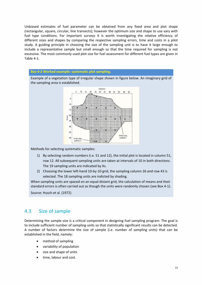
Box 4‐2 Worked example: systematic plot sampling.
Example of a vegetation type of irregular shape shown in figure below. An imaginary grid of the sampling area is established.
Methods for selecting systematic samples:
1) By selecting random numbers (i.e. 51 and 12), the initial plot is located in column 51,
row 12. All subsequent sampling units are taken at intervals of 10 in both directions.
The 19 sampling units are indicated by Xs.
2) Choosing the lower left‐hand 10‐by‐10 grid, the sampling column 26 and row 43 is
selected. The 18 sampling units are indicted by shading.
When sampling units are spaced on an equal distant grid, the calculation of means and their standard errors is often carried out as though the units were randomly chosen (see Box 4‐1).
Source: Husch et al. (1972)
4.3 Size of sample
Determining the sample size is a critical component in designing fuel sampling program. The goal is to include sufficient number of sampling units so that statistically significant results can be detected. A number of factors determine the size of sample (i.e. number of sampling units) that can be established in the field, namely:
method of sampling
variability of population
size and shape of units
time, labour and cost.
14
Of these factors, the last (time, labour and cost) is often the most critical and frequently overrides the desired number of units calculated using the standard formulae (see Box 4.3), i.e. due to cost, fewer than desired have to be accepted.
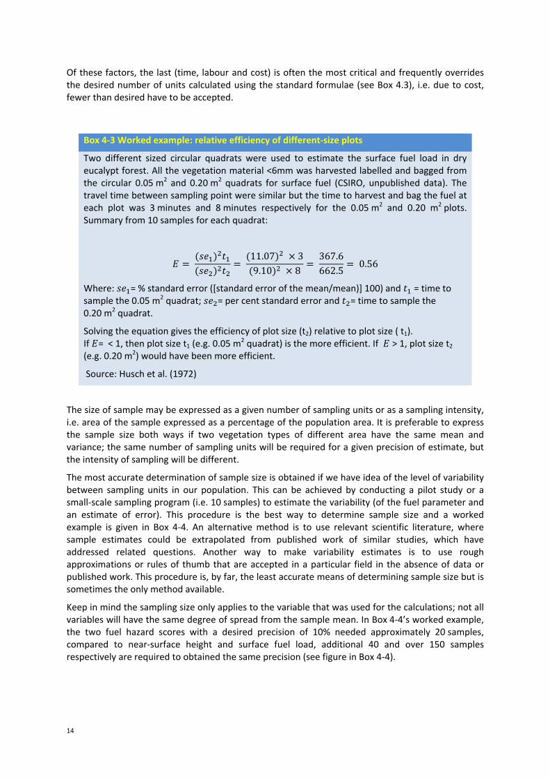
Box 4‐3 Worked example: relative efficiency of different‐size plots
Two different sized circular quadrats were used to estimate the surface fuel load in dry eucalypt forest. All the vegetation material <6mm was harvested labelled and bagged from the circular 0.05 m2 and 0.20 m2 quadrats for surface fuel (CSIRO, unpublished data). The travel time between sampling point were similar but the time to harvest and bag the fuel at each plot was 3 minutes and 8 minutes respectively for the 0.05 m2 and 0.20 m2 plots. Summary from 10 samples for each quadrat:
11.07 39.10 8
367.6662.5
0.56
Where: = % standard error ([standard error of the mean/mean)] 100) and = time to sample the 0.05 m2 quadrat; = per cent standard error and = time to sample the 0.20 m2 quadrat.
Solving the equation gives the efficiency of plot size (t2) relative to plot size ( t1). If = < 1, then plot size t1 (e.g. 0.05 m
2 quadrat) is the more efficient. If > 1, plot size t2 (e.g. 0.20 m2) would have been more efficient.
Source: Husch et al. (1972)
The size of sample may be expressed as a given number of sampling units or as a sampling intensity, i.e. area of the sample expressed as a percentage of the population area. It is preferable to express the sample size both ways if two vegetation types of different area have the same mean and variance; the same number of sampling units will be required for a given precision of estimate, but the intensity of sampling will be different.
The most accurate determination of sample size is obtained if we have idea of the level of variability between sampling units in our population. This can be achieved by conducting a pilot study or a small‐scale sampling program (i.e. 10 samples) to estimate the variability (of the fuel parameter and an estimate of error). This procedure is the best way to determine sample size and a worked example is given in Box 4‐4. An alternative method is to use relevant scientific literature, where sample estimates could be extrapolated from published work of similar studies, which have addressed related questions. Another way to make variability estimates is to use rough approximations or rules of thumb that are accepted in a particular field in the absence of data or published work. This procedure is, by far, the least accurate means of determining sample size but is sometimes the only method available.
Keep in mind the sampling size only applies to the variable that was used for the calculations; not all variables will have the same degree of spread from the sample mean. In Box 4‐4’s worked example, the two fuel hazard scores with a desired precision of 10% needed approximately 20 samples, compared to near‐surface height and surface fuel load, additional 40 and over 150 samples respectively are required to obtained the same precision (see figure in Box 4‐4).

15
Table 4‐1. Plot sizes used in bushfire fuel sampling in selected fuel types
Fuel type Fuel parameter Shape Size Area Reference
Grassland fuel load rectangular 0.3 m 0.6 m 0.18 m2 Cheney et al. 1993
Forest litter fuel load circular 252.3 mm dia. 0.05 m2 Cheney et al. 1990, 1992; Gould 2007a, 2011;
McCaw 2011 square 0.5 m 0.5 m 0.25 m2 DENR 2011
square 1 m 1 m 1.0 m2 Marsden‐Smedley and Anderson 2011
near‐surface fuel load circular 505 mm dia. 0.20 m2 Gould et al. 2007a, 2011 elevated fuel load rectangular 1 m 2 m 2 m2 Cheney et al. 1992; Gould 2007a
rectangular 1 m 4 m 4 m2 Cheney et al. 1990
visual fuel hazard assessment (surface, near‐surface, elevated)
circular 5 m radius 78.6 m2 Gould et al. 2007b, 2011; Watson et al. 2012
circular 10 m radius 314.3 m2 DENR 2011 visual fuel hazard
assessment (bark) circular 10 m radius 314.3 m2 Gould et al., 2007b, 2011; DENR, 2011; Watson et al.
2012 Mallee heath fuel load rectangular 1 m 2 m 2 m2 Cruz et al. 2010
square 1 m 1 m 1 m2 McCaw 1997
visual fuel hazard assessment (surface, near‐surface, elevated)
circular 5 m radius 78.6 m2 Cruz et al. 2010
Visual fuel hazard assessment intermediate and overstorey canopy
circular 10 m radius 314.3 m2 Cruz et al. 2010
Buttongrass moorland
fuel load square 2 m 2 m 4 m2 Marsden‐Smedley and Catchpole 1995b;
16
Box 4‐4 Worked example: size of sample
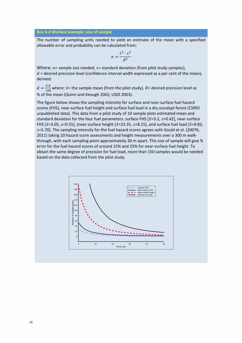
The number of sampling units needed to yield an estimate of the mean with a specified allowable error and probability can be calculated from:
∙
Where: = sample size needed, = standard deviation (from pilot study samples),
= desired precision level (confidence interval width expressed as a per cent of the mean), derived:
∙ where: = the sample mean (from the pilot study), = desired precision level as
% of the mean (Quinn and Keough 2002; USDI 2003).
The figure below shows the sampling intensity for surface and near‐surface fuel hazard scores (FHS), near‐surface fuel height and surface fuel load in a dry eucalypt forest (CSIRO unpublished data). This data from a pilot study of 10 sample plots estimated mean and standard deviation for the four fuel parameters: surface FHS [ =3.2, =0.42], near‐surface FHS [ =3.05, =0.55], (near‐surface height [ =23.35, =8.15], and surface fuel load [ =9.82, =5.70]. The sampling intensity for the fuel hazard scores agrees with Gould et al. (2007b, 2011) taking 10 hazard score assessments and height measurements over a 300 m walk‐through, with each sampling point approximately 30 m apart. This size of sample will give % error for the fuel hazard scores of around 15% and 25% for near‐surface fuel height. To obtain the same degree of precision for fuel load, more than 150 samples would be needed based on the data collected from the pilot study.
5 10 15 20 25 30
Error (%)
0
20
40
60
80
100
120
140
160
180
200
Num
ber
of s
ampl
e p
oint
s
Surface FHSNear-surface FHSNear-surface heightSurface fuel load
17
4.4 Destructive fuel sampling
Several methods have been used to estimate biomass of bushfire fuels in various fuel types (Burrows and McCaw 1990; Burrows et. al. 1991; Catchpole and Wheeler 1993; Cheney et al. 1990, 1992, 1993; Cruz 2010; Gould et al. 2007a, 2011; Marsden‐Smedley and Catchpole 1995b; McCaw 1997). The common techniques of destructive sampling involve the removal/harvest of fuel and/or vegetation from the sampling unit for later assessment. This assessment involves sorting, drying and weighing the sample to express the samples in terms of oven‐dried (at nominal 100 oC temperature for 24 hours) weight per unit area (e.g. kg m2 or t ha‐1). Destructive sampling gives an accurate measure of biomass at a particular sampling point. However, the inherent inaccuracies are introduced by making estimates over a larger area and good sampling design is required to overcome this problem (Catchpole and Wheeler 1992).
The disadvantage of destructive sampling is the inherent cost associated with its high labour requirements. In addition, the time‐consuming procedures of locating a plot, harvesting, sorting, and drying are not useful in situations where a quick estimated is required—for example, for real‐time fire predictions. Consequently, sample site selection and number of samples are often insufficient to account for the variability of the vegetation and so the error in generalising to a large area can be substantial (Catchpole and Wheeler 1992).
Sampling different fuel strata and vegetation types will require different sampling intensities and sample plot size. The precision of the estimates of biomass obtained from destructive sampling decreases as the spatial variation of the vegetation increases, so the sample quadrat need to increase in size. For this reason, small sampling quadrats are more suitable for forest litter and grass fuel (i.e. < 1 m2) and in sparse or discontinuous fuels, larger sampling units are needed, typically > 2 m2 (see Table 4‐1).
Catchpole and Wheeler (1992) discussed a ranked sampling technique, which increases the efficiency of destructive sampling described by McIntyre (1952). Van Loon (1977), Cheney et al. (1992) and Gould et al. (2007a, 2011), have used this technique for sampling forest litter fuel fuels. The ranked sampling study by Gould et al. (2007a) identified surface fuel layer at each sampling point, and within a 5‐m radius of the sample point, the fuel sampler bias was removed by visually ranking both layers in order of light, medium and heavy fuel loads. The surface fuel litter depth and a small 0.05 m2 sample of all material < 6 mm was taken at each ranking. The result was no significant difference between the mean of the three ranked samples and the mean of the medium sample alone. Therefore, the efficiency of destructive sampling of surface fuel can be obtained by ranking the fuels load light, medium and heavy at each sampling point and only destructive sample the medium‐ranked sample (Gould et al. 2007a).
In Catchpole and Wheeler (1992), Morris (1958) showed that for a fixed sampling area the information obtained from a site increases as the quadrat size decreases. They argue that work per unit area will generally increase as quadrat size decreases; hence, the number of quadrats increases. Box 4‐3 gives a worked example showing that sampling efficiency is better with a greater number of smaller quadrats (rather than fewer large quadrats) to obtain the sample precision, thus more samples will give a better representation of the site biomass.
18
4.5 Non‐destructive sampling
In non‐destructive sampling the sampling unit is searched or sampled in situ. This can be advantageous, because less labour and time is required than for destructive methods. Commonly used, non‐destructive sampling can ranged from simple rapid visual assessments to highly detailed measurements or tallies of complex fuel beds along transect lines (Davis et al. 2008; Sikkink and Keane 2008). Over the years there been several distinct types of non‐sampling techniques developed to sample vegetation cover, coarse woody debris, curing, fuel hazard ratings and fuel loads.
4.5.1 VISUAL FUEL ASSESSMENT
Over the past decade in Australia the application of visual fuel hazard ratings to assess the fuel factors affecting fire behaviour and suppression difficulties (DEH 2006, 2011; Gould et al.2007b, 2011; Hines et al. 2010; McCarthy et al. 1999, Tolhurst et al. 1996; Wilson 1992, 1993). These techniques emphasise hazard rating attributes based on fuel structure, continuity, amount of dead material and particle size for each of the different fuel layers i.e. bark, elevated (shrub fuels), near‐surface fuel (suspended litter) and surface fuels (forest litter fuels)in dry eucalypt forest and shrub heath fuel types. Fuel hazard guides and their
ratings (commonly known as Overall Fuel Hazard GuideHines et al. 2011;McCarthy et al. 1999) or scores
(commonly known as Vesta fuel hazard scoresGould et al. 2007b, 2011) have been used to predict rate of spread based on other fire behaviour parameters as fuels develop with age (Cheney et al. 2012; Gould 2007a, 2007b).
Most of the agencies in the eastern states adopted the Victorian Government Department of Sustainability and Environment (DSE) Overall Fuel Hazard Guide (Hines et al. 2010; McCarthy et al. 1999) for forest fuel assessments. South Australia (DENR 2011) developed their own fuel hazard guide based on McCarthy et al. (1999), Gould et al. (2007) and Hines et al. (2010) (see Appendix B). The field procedures for assessment of the fuels varied widely between agencies and in some case within agencies, with no consistent sampling procedures or guidelines for the visual assessment of fuel hazard. These guides provide a description for each fuel stratum. Practitioners can apply these guides along with a good sampling design to make rapid and consistent assessments of fuel hazard ratings in a range of dry eucalypt forests given in Box 4‐5.
Box 4‐5 Worked example: visual fuel hazard assessment
Fuel hazard score/rating should be calculated as the average of 10 samples and height measurements over a 300 m walk through of a block or compartment (i.e. 200 ha area). At each sampling point (approximately 30 m apart), the surface and near‐surface and elevated fuel is visually assessed for its fuel hazard rating/score within a 5‐m radius of the sample point. The average depth/top‐height of the surface, near‐surface and elevated fuel measured and recorded. Bark fuel is visually assessed within a 10‐m radius of the sample rating/score is noted. The sample of 10 should give a good estimate of the fuel hazard rating (see Box 4‐4). Larger compartment will require more sampling units.
4.5.2 PHOTO KEY VISUAL ASSESSMENT
The most common visual assessment technique is the photo series method, with a wide range of applications in estimating fuel load, per cent cover, grass curing, fuel hazard, etc. Photo series are a common practice in the United States, with the initial development by Maxwell and Ward (1976), and implemented by Fischer (1981a and b) and Ottmar et al. (2000). In the photo series method, fuel loads for disparate forest and rangeland are photographed using oblique photographs, then the forest and rangeland settings are sampled and quantified (Sandberg et al. 2001; Fischer 1981b). Theoretically, the load values are then applied to sites that appear visually similar. Fuel loads in new study areas are estimated by visually
19
matching observed fuel bed conditions with these photographs (Keane and Dickinson 2007a, b; Sikkink and Keane 2008).
Grassland curing refers to a measure of grass greenness and relates to the per cent of grass material that is dead in the sward. Visual assessments of grass curing relies on field observers to estimate the percentage curing, based on expert judgement and often with the aid of visual guides (Anderson et al. 2011). The Country Fire Authority (Victoria) first initiated a photo key for assessment of grassland curing (CFA 1987). Since then, there has been increasing development and use of photo key series over the past decade in Australia. A number of agencies have developed local or regional field guides for grassland curing and estimating fuel loads (CFA 1987, 2001; FESA 2007a, b, 2008, 2009, and 2010 a, b, c ; Johnson 2002). The majority of these photo guides provided limited information or data on how the estimates were obtained in relationship to the photograph. The photograph examples in the fuel hazard field guides are not photographic guides (e.g. DEHR 2011; Gould et al. 2007b; Hines et al. 2010; McCarthy et al. 1999) because the photographs cannot adequately show all of the key attributes that are important in determining fuel hazard (Gould et al. 2007b; Hines et al. 2010).
Photo key assessment varies in complexity, from simple illustrated photographic examples of the fuel complex with associated fuel attributes (e.g. Anderson 1982; Taylor et al. 1996) to detail of stereo pairs and photoload series (Ottmar et al. 1998, 2000; Keane and Dickinson 2007a, b). Field guides with stereo‐pair photographs viewed with a stereoscope improve the ability to appraise natural fuels, vegetation and stand structure conditions. These photographic images accompanied with detailed understorey fuel inventory have applications in several branches in conservation and natural resource land management. Examples of photographic images with supporting ground inventory data are useful for evaluating and monitoring fuel types or vegetation communities. Fire managers will find these data useful for predicant fuel consumption, smoke production, fire behaviour and fire effects during wildfires and prescribed fires. In addition, a photo series can be used to appraise carbon sequestration, an important factor in prediction of future climate, and link remotely sensed signatures to live and dead fuels on the ground (Ottmar et al. 1998). The photographs and accompanying data from detail sampling of the key fuel attributes from transect lines, destructive samples and trees and shrubs counts.
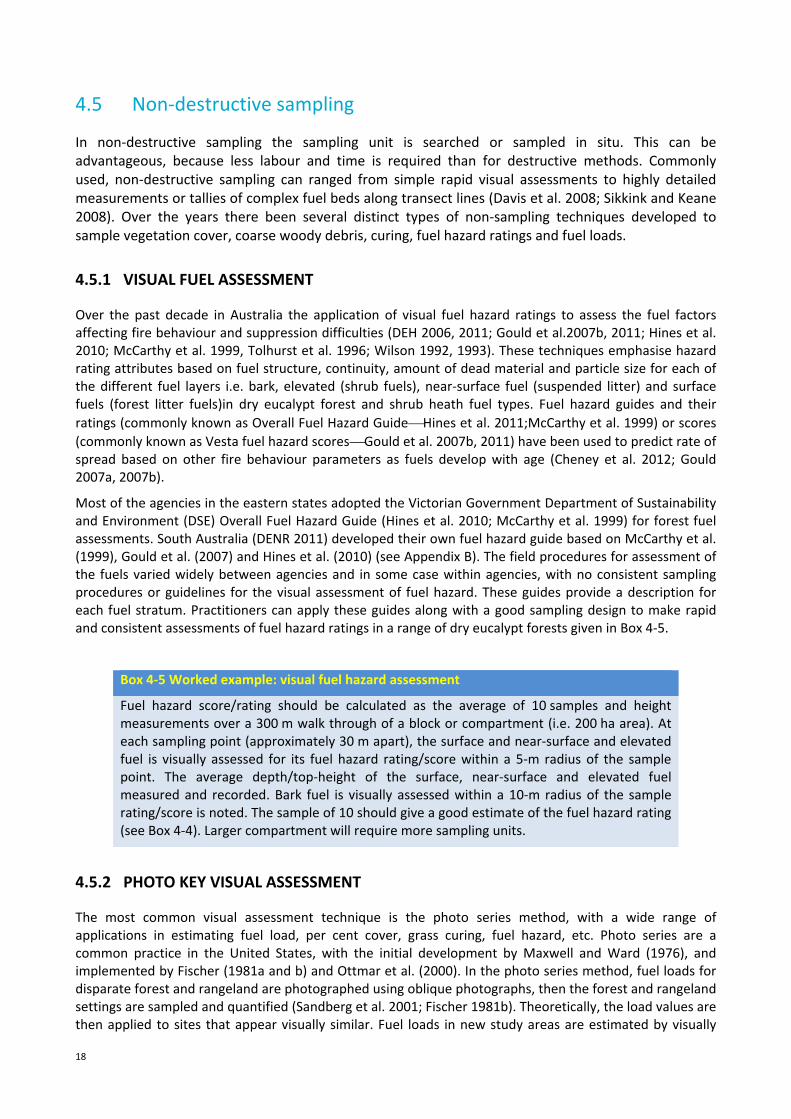
Keane and Dickinson (2007a) developed a photoload sampling technique that quickly and accurately estimates surface fuel component loading using visual assessment of loading referencing a sequence of downward looking photographs depicting graduated fuel loadings by fuel component. The development of photoload sequenced involve:
1) collecting the fuel to be photographed in the field and bringing them back to the laboratory to
measure dry weights and density
2) constructing the fuel beds in sequential series of increasing fuel load for each component
3) photographing these fuels in a reference quadrat (e.g. fine fuels m2 quadrant)
4) compiling the photographs into a decision support systems along with sampling design for field
application.
Figure 4‐1 is an example of a photoload sequence for the 1 hr fuel component for conifer litter fuel (Keane and Dickinson 2007b).
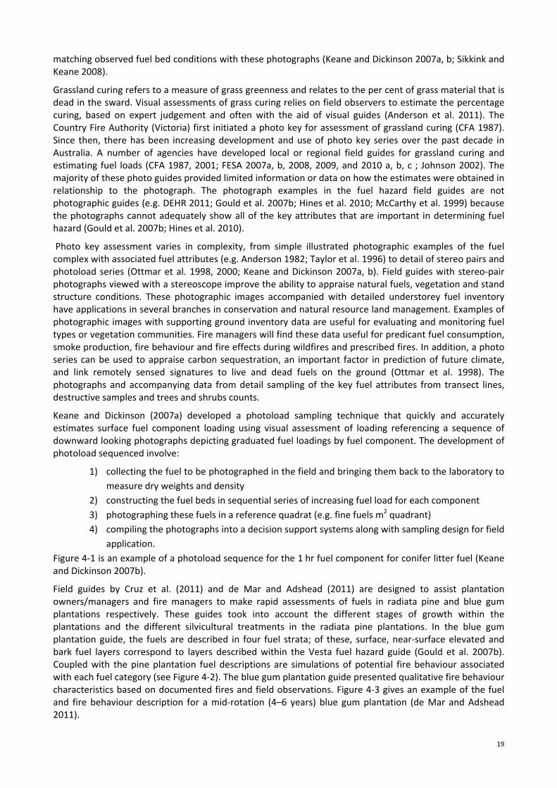
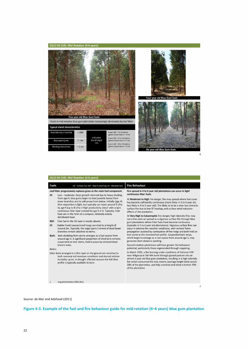
Field guides by Cruz et al. (2011) and de Mar and Adshead (2011) are designed to assist plantation owners/managers and fire managers to make rapid assessments of fuels in radiata pine and blue gum plantations respectively. These guides took into account the different stages of growth within the plantations and the different silvicultural treatments in the radiata pine plantations. In the blue gum plantation guide, the fuels are described in four fuel strata; of these, surface, near‐surface elevated and bark fuel layers correspond to layers described within the Vesta fuel hazard guide (Gould et al. 2007b). Coupled with the pine plantation fuel descriptions are simulations of potential fire behaviour associated with each fuel category (see Figure 4‐2). The blue gum plantation guide presented qualitative fire behaviour characteristics based on documented fires and field observations. Figure 4‐3 gives an example of the fuel and fire behaviour description for a mid‐rotation (4–6 years) blue gum plantation (de Mar and Adshead 2011).
20
Source: Keane and Dickinson (2007b)
Figure 4‐1. An example of a photoload sequence for the 1‐hr fuel component
21
Source: Cruz et al. (2011)
Figure 4‐2. Example of the fuel and fire behaviour guide for pruned radiata pine plantation 4–8 years old
22
Source: de Mar and Adshead (2011)
Figure 4‐3. Example of the fuel and fire behaviour guide for mid‐rotation (4–6 years) blue gum plantation
23
Multimedia tools such as virtual reality (VR) photography have considerable potential for enhancing understanding needs in fuel assessment. The 360° interactive image allows the viewer to obtain virtual 360° images of field sites and holds much promise for education and training delivery in this field. Panoramic photographs are wide pictures that show at least as much horizontally as the eye is capable of seeing and usually include more of the viewer’s peripheral vision. Panoramic images are popular in virtual reality applications and now appear increasingly on number of web sites. VR photography is a technique of capturing or creating a complete scene as a single image, as viewed when rotating about a single central position. Normally created by stitching together a number of photographs taken in a multi‐row 360° rotation, the complete image can also be a totally computer‐generated effect, or a composite of photography and computer generated objects.
VR panoramas are usually viewed through movie players, such as Apple’s QuickTime software. Application of the VR panoramas was used during Project Vesta implementation training throughout Australia in 2008 (JS Gould, CSIRO and WL McCaw, DEC WA pers. comm.), using examples of VR images of different fuel types for training purpose. The VR panoramas have potential to aid in fuel assessment in the field if linked to tablet applications. They also show great promise to allow users to contrast different fuel structures or hazard ratings; these could be used for training and linked to a web knowledge base (e.g. the proposed WikiFuel in Section 2).
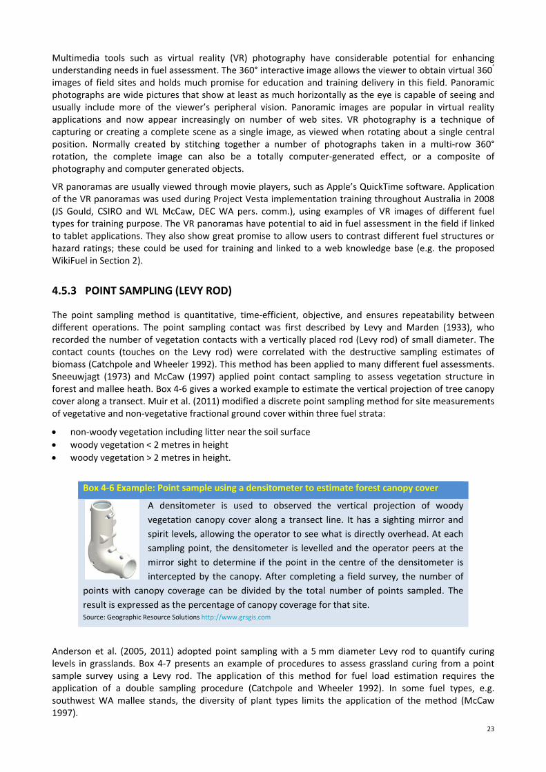
4.5.3 POINT SAMPLING (LEVY ROD)
The point sampling method is quantitative, time‐efficient, objective, and ensures repeatability between different operations. The point sampling contact was first described by Levy and Marden (1933), who recorded the number of vegetation contacts with a vertically placed rod (Levy rod) of small diameter. The contact counts (touches on the Levy rod) were correlated with the destructive sampling estimates of biomass (Catchpole and Wheeler 1992). This method has been applied to many different fuel assessments. Sneeuwjagt (1973) and McCaw (1997) applied point contact sampling to assess vegetation structure in forest and mallee heath. Box 4‐6 gives a worked example to estimate the vertical projection of tree canopy cover along a transect. Muir et al. (2011) modified a discrete point sampling method for site measurements of vegetative and non‐vegetative fractional ground cover within three fuel strata:
non‐woody vegetation including litter near the soil surface
woody vegetation < 2 metres in height
woody vegetation > 2 metres in height.
Box 4‐6 Example: Point sample using a densitometer to estimate forest canopy cover
A densitometer is used to observed the vertical projection of woody
vegetation canopy cover along a transect line. It has a sighting mirror and
spirit levels, allowing the operator to see what is directly overhead. At each
sampling point, the densitometer is levelled and the operator peers at the
mirror sight to determine if the point in the centre of the densitometer is
intercepted by the canopy. After completing a field survey, the number of
points with canopy coverage can be divided by the total number of points sampled. The
result is expressed as the percentage of canopy coverage for that site. Source: Geographic Resource Solutions http://www.grsgis.com
Anderson et al. (2005, 2011) adopted point sampling with a 5 mm diameter Levy rod to quantify curing levels in grasslands. Box 4‐7 presents an example of procedures to assess grassland curing from a point sample survey using a Levy rod. The application of this method for fuel load estimation requires the application of a double sampling procedure (Catchpole and Wheeler 1992). In some fuel types, e.g. southwest WA mallee stands, the diversity of plant types limits the application of the method (McCaw 1997).
24
Box 4‐7 Worked example: Point sample (Levy rod) to quantify grassland curing
Levy touch method to estimate grass curing:
1. Obtain equipmenta Levy rod (a steel rod 1.3 m high, 3.5–5 mm in diameter, with
tip fashioned into a point), 50 m tape, clipboard and booking sheets.
2. Select a site that is representative of the overall area with respect to slope, aspect
and grass species. Site on level terrain is preferred. Allow enough area to fit a
50 mtransect line.
3. Stretch out the 50‐m tape, and along it at each 1‐m interval, strike the levy rod
vertically to the ground. It is important that the Levy rod is as close to perpendicular
to the ground as possible to ensure an accurate representation of the vertical grass
profile.
4. Record all contacts made with the road starting from the highest contact to the
lowest.
5. Record the contacts as live and dead.
6. Move to the next 1‐m interval and repeat the process, continuing for the length of
the transect line.
7. Grass curing is then determined through the following formula:
degree of curing (%) = (total dead touches/total touches) x 100 Sources: Anderson et al. (2005, 2011)
4.5.4 LINE TRANSECT INTERSECT
Line transect intersect was originally introduced by Warren and Olsen (1964), and was made applicable to measuring coarse woody debris (CWD) by Van Wagner (1968). In this method the diameter of CWD is measured at the point of intersection along a transect line of a given length but no width. Several variation of the original technique that vary the line arrangements i.e. length, transect layout, and number of replicates (Brown 1974; DeVries 1974; Hansen 1996; Hollis et al. 2010; Michs et al. 2009; Nemec‐Linnel and Davis 2002; Slijepcevic and Marsden‐Smedley 2002; Slijepcevic 2011; Woldendorp et al. 2004).
As the frequency of CWD generally increases with decreasing diameter size, some line transect intersect designs determine the length of the transect line to be sampled by the diameter of the woody debris, particularly when fine wood debris is included (Delisel et al. 1988; USDA Forest Service 2001). In this methods, transects are divided into sections and measurement on these section correspond to diameter size classes, i.e. all woody debris measured on the first section of the transect line, and then for each subsequent section, the smallest diameter class is disregarded. This ensures that over‐sampling does not occur for the small‐sized wood pieces, and that a sufficient number of the largest‐sized pieces are sampled (Woldendorp et al. 2004).
Transects are often arranged in different orientation at a site to reduce potential for orientation bias. Thus, many layout variants have been adopted, including an equilateral triangle (Delisle et al. 1998; Marshall et al. 2000; Nemec‐Linnell and Davis 2002), three transects radiating from a common point (Nemec‐Linnell and Davis 2002; Waddell 2002), a square, an ‘L’ shape, a single line (Bell et al. 1996) and variations of these (Nemec‐Linnell and Davis 2002). Bell et al. (1996) conclude that there is no advantage in using one transect arrangement over another if CWD pieces are orientated at random. Therefore, at sites with randomly orientated CWD pieces there is no apparent benefit in using a methodology with a complex transect arrangement if a single line transect will be quicker to implement and will provide similar results. A worked sample of a line intersect transect based on methods from Van Wagner (1969) and Brown (1974) on a sub‐sample of data from Hollis et al. (2010) is given in Box 4‐8.

25
Box 4‐8 Worked example: line transect intercept to estimate coarse woody debris (CWD) load (t ha‐1)
Sampling procedures:
1. Lay a line transect of known length across area to be sampled.
2. Record the diameter of every piece of coarse woody debris (e.g. > 2.5 cm diameter)
if the line transect crosses the central axis of the CWD:
a. for straight piece of CWD crossed once, the diameter is measured at point
of intersection
b. for line transect that did not include the central axis, do not tally
c. for a piece of CWD crossed twice because it is branched, treat as two
separate pieces, with diameter measured at each point of intersection
d. for a piece of CWD crossed three times because it is crooked, measure
diameter at each point of intersection (the transect line is shown as a
dashed line in figure below).
Worked example from Hollis (2010) 25 m transect line (L) with recorded diameters (di, cm): 2.9, 2.8, 2.6, 3.2, 3.2, 5.0, 4.2, 2.6, 4.0, 2.8, 7.0, 3.5, 3.8, 13.0, 19.4, 7.3, 2.7, 16.0, 2.6, 2.6, 8.30, 6.5, 3.5, 3.8
Calculate the CWD load (W, t ha‐1) from Brown’s (1974) formula:
∙8
where: is the wood density (0.56697 g cm‐3, Hollis 2010)
0.566978 25
2.9 2.8 2.6 ⋯ 3.8
35.7tha‐1
Sources: Brown (1974); Hollis et al. (2010); Van Wagner (1968)
4.5.5 SUMMARY
In this section, we have provided an overview of the philosophy of sampling, the rationale behind the choice of sample units and technique, and some assistance to determine what is the best sampling method to use in particular situations. We have not provided detailed mathematical and statistical formulae, but
26
have given worked examples of some basic principles used in designing a fuel assessment program. Those wishing to explore more of the statistical and mathematical background should consult relevant textbooks such as Cochran (1977), Johnson (2000) and Ardilly and Tillé (2006).
4.6 Fuel dynamic models
Fuel characteristics are temporally and spatially complex and can vary widely across the landscape. These characteristics can affect fire spread, flame structure and duration and intensity of bushfires. Describing and quantifying fuel is important for understanding fire behaviour and also provides information to support fire management activities including prescribed burning, suppression difficulty, fuel hazard assessment and fuel treatment. The amount and arrangement of fuel available that actually burns under prevailing weather conditions is one of the most important factors in determining the fire behaviour and fuel management. This depends on the moisture content and characteristics of the fuel (i.e. structure, composition, continuity and load), which has accumulated over time since last fire. The dynamics of available fuel are important for:
Determining the quantity of fuel at a particular time since last fire. An increase in fuel availability
has a dramatic effect on rate of spread and intensity of forest fires. For example in dry sclerophyll
forest, doubling fuel load will double rate of spread and quadruple fire intensity (Peet 1965;
McArthur 1967)
Assessing the effectiveness of prescribed burning for fuel management, i.e. to determine the
period of effective fuel reduction (Raison et al. 1983).
Accumulation of fine surface fuels after fire depends on the difference between the rate of accession and decomposition of litter, while the build up of the near‐surface fuel and elevated fuel layers depends on the rate of net biomass production of the understorey vegetation. The pattern of fuel accumulation after fire in Australia varies widely with forest type and environmental conditions (Birk and Simpson 1980; Burrows 1994; Conroy 1994; Raison et al. 1983, 1986; Walker 1981). These authors developed models describing the pattern and rate build up of litter fuels after burning, following the general form of an exponential function rising to a maximum or steady‐state fuel load:
wt = wss(1‐e‐kt) Equation (1)
where wt is the weight (e.g. kg m‐2) of the litter accumulated at time t (years); wss is the amount of fuel
accumulated under steady‐state conditions, and k is the decomposition constant. This model has been adapted from the model proposed by Olson (1963) to describe the relationship between decomposition and accumulation. The general pattern of fuel accumulation in dry eucalypt forest described by this model is one of relatively rapid and steady accumulation for a period following fire, commonly 5 to 8 years, after which time the rate of accumulation declines progressively and fuel loading stabilises at a level in equilibrium with the prevailing environmental conditions. Walker (1981) discussed this function and described a curve that flattens out to a plateau or steady state which tends to be greater in more productive forests, and is generally proportional to canopy cover within a particular forest type (Fox et al. 1979; Birk and Simpson 1980; Burrows 1994; O’Connell 1987; Raison et al. 1983). This is also supported by the work of O’Connell (1987), who developed a mechanistic model to predict accumulation of forest‐floor litter based on measured rates of litter‐fall together with decay constants that were derived from exponential decay models and ten karri (E. diversicolor) forest‐litter fractions.
The pattern of litter fuel accumulation after fires varies widely from year to year with forest type and environmental conditions (Simmons and Adams 1986; Walker 1981). Characteristics of these litter fuel accumulation curves have been established for some eucalypt forest types (see Figure 4‐4 and Table 4‐2). The fuel load in dry sclerophyll forest with 50 per cent canopy cover builds up rapidly for the first 10 years and then reaches an equilibrium fuel load of about 15 t ha‐1 by about 15 years ( Burrows 1994; Gould 1996; Gould et al. 2011; Raison et al. 1983). If there is a substantial layer of shrubs, the elevated fuel load may still be increasing 25 years after burning (Van Loon 1977).
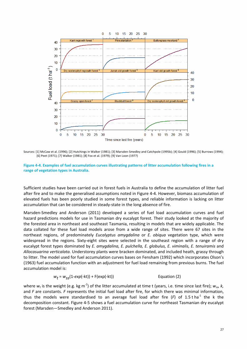
27
Sources: [1] McCaw et al. (1996); [2] Hutchings in Walker (1981); [3] Marsden‐Smedley and Catchpole (1995b); [4] Gould (1996); [5] Burrows (1994); [6] Peet (1971); [7] Walker (1981); [8] Fox et al. (1979); [9] Van Loon (1977)
Figure 4‐4. Examples of fuel accumulation curves illustrating patterns of litter accumulation following fires in a range of vegetation types in Australia.
Sufficient studies have been carried out in forest fuels in Australia to define the accumulation of litter fuel after fire and to make the generalised assumptions noted in Figure 4‐4. However, biomass accumulation of elevated fuels has been poorly studied in some forest types, and reliable information is lacking on litter accumulation that can be considered in steady‐state in the long absence of fire.
Marsden‐Smedley and Anderson (2011) developed a series of fuel load accumulation curves and fuel hazard predictions models for use in Tasmanian dry eucalypt forest. Their study looked at the majority of the forested area in northeast and southeast Tasmania, resulting in models that are widely applicable. The data collated for these fuel load models arose from a wide range of sites. There were 67 sites in the northeast regions, of predominately Eucalyptus amygdalina or E. obiqua vegetation type, which were widespread in the regions. Sixty‐eight sites were selected in the southeast region with a range of dry eucalypt forest types dominated by E. amygdalina, E. pulchella, E. globulus, E. viminalis, E. tenuiramis and Allocasuarina verticalata. Understorey plants were bracken dominated, and included heath, grassy through to litter. The model used for fuel accumulation curves bases on Fensham (1992) which incorporates Olson’s (1963) fuel accumulation function with an adjustment for fuel load remaining from previous burns. The fuel accumulation model is:
wt = wss(1‐exp(‐kt)) + F(exp(‐kt)) Equation (2)
where wt is the weight (e.g. kg m‐2) of the litter accumulated at time t (years, i.e. time since last fire); wss, k,
and F are constants. F represents the initial fuel load after fire, for which there was minimal information, thus the models were standardised to an average fuel load after fire (F) of 1.5 t ha‐1 the k the decomposition constant. Figure 4‐5 shows a fuel accumulation curve for northeast Tasmanian dry eucalypt forest (Marsden—Smedley and Anderson 2011).
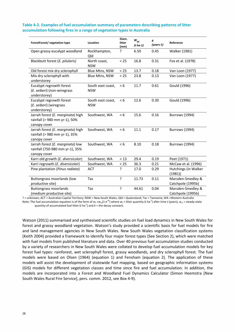
28
Table 4‐2. Examples of fuel accumulation summary of parameters describing patterns of litter accumulation following fires in a range of vegetation types in Australia
ForestForest/ vegetation type Location Diam. litter (mm)
Wss (t ha‐1)
K (years‐1)
Reference
Open grassy eucalypt woodland Rockhampton, Qld
? 6.50 0.45 Walker (1981)
Blackbutt forest (E. pilularis) North coast, NSW
< 25 16.8 0.31 Fox et al. (1978)
Old forest mix dry sclerophyll Blue Mtns, NSW < 25 13.7 0.18 Van Loon (1977)
Mix dry sclerophyll with understorey
Blue Mtns, NSW < 25 23.8 0.13 Van Loon (1977)
Eucalypt regrowth forest (E. seiberi) (non‐wiregrass understorey)
South east coast, NSW
< 6 11.7 0.61 Gould (1996)
Eucalypt regrowth forest (E. seiberi) (wiregrass understorey)
South east coast, NSW
< 6 12.6 0.30 Gould (1996)
Jarrah forest (E. marginata) high rainfall (> 980 mm yr‐1), 50% canopy cover
Southwest, WA < 6 15.6 0.16 Burrows (1994)
Jarrah forest (E. marginata) high rainfall (> 980 mm yr‐1), 35% canopy cover
Southwest, WA < 6 11.1 0.17 Burrows (1994)
Jarrah forest (E. marginata) low rainfall (750‐980 mm yr‐1), 35% canopy cover
Southwest, WA < 6 8.10 0.18 Burrows (1994)
Karri old growth (E. diversicolor) Southwest, WA < 13 29.4 0.19 Peet (1971)
Karri regrowth (E. diversicolor) Southwest, WA < 25 36.3 0.21 McCaw et al. (1996)
Pine plantation (Pinus radiata) ACT ? 17.0 0.29 Hutchings (in Walker (1981))
Buttongrass moorlands (low productive site)
Tas ? 11.73 0.11 Marsden‐Smedley & Catchpole (1995b)
Buttongrass moorlands (medium productive site)
Tas ? 44.61 0.04 Marsden‐Smedley & Catchpole (1995b)
? = unknown; ACT = Australian Capital Territory; NSW = New South Wales; Qld = Queensland; Tas = Tasmania; WA =Western Australia Note: The fuel accumulation equation is of the form of wt =wss(1‐e
‐kt) where wt = litter quantity (t ha
‐1) after time t (years), wss = steady‐state
quantity of accumulated fuel litter (t ha‐1) and k = the decay constant.
Watson (2011) summarised and synthesised scientific studies on fuel load dynamics in New South Wales for forest and grassy woodland vegetation. Watson’s study provided a scientific basis for fuel models for fire and land management agencies in New South Wales. New South Wales vegetation classification systems (Keith 2004) provided a framework to identify four major forest types (See Section 2), which were matched with fuel models from published literature and data. Over 40 previous fuel accumulation studies conducted by a variety of researchers in New South Wales were collated to develop fuel accumulation models for key forest fuel types: rainforest, wet sclerophyll forest, grassy woodlands, and dry sclerophyll forest. The fuel models were based on Olsen (1964) (equation 1) and Fensham (equation 2). The application of these models will assist the development of statewide fuel mapping, based on geographic information systems (GIS) models for different vegetation classes and time since fire and fuel accumulation. In addition, the models are incorporated into a Forest and Woodland Fuel Dynamics Calculator (Simon Heemstra [New South Wales Rural Fire Service], pers. comm. 2012, see Box 4‐9).
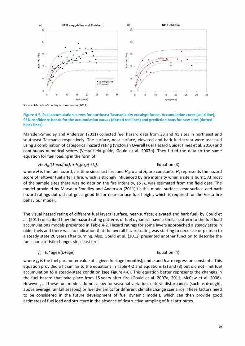
29
Source: Marsden‐Smedley and Anderson (2011)
Figure 4‐5. Fuel accumulation curves for northeast Tasmania dry eucalypt forest. Accumulation cures (solid line), 95% confidence bands for the accumulation curves (dotted red lines) and prediction bans for new sites (dotted black lines)
Marsden‐Smedley and Anderson (2011) collected fuel hazard data from 33 and 41 sites in northeast and southeast Tasmania respectively. The surface, near‐surface, elevated and bark fuel strata were assessed using a combination of categorical hazard rating (Victorian Overall Fuel Hazard Guide, Hines et al. 2010) and continuous numerical scores (Vesta field guide, Gould et al. 2007b). They fitted the data to the same equation for fuel loading in the form of
H= Hss((1‐exp(‐kt)) + Ho(exp(‐kt)), Equation (3)
where H is the fuel hazard, t is time since last fire, and Hss, k and Ho are constants. Ho represents the hazard
score of leftover fuel after a fire, which is strongly influenced by fire intensity when a site is burnt. At most
of the sample sites there was no data on the fire intensity, so Ho was estimated from the field data. The
model provided by Marsden‐Smedley and Anderson (2011) fit this model surface, near‐surface and bark
hazard ratings but did not get a good fit for near‐surface fuel height, which is required for the Vesta fire
behaviour model.
The visual hazard rating of different fuel layers (surface, near‐surface, elevated and bark fuel) by Gould et al. (2011) described how the hazard rating patterns of fuel dynamics have a similar pattern to the fuel load accumulations models presented in Table 4‐2. Hazard ratings for some layers approached a steady state in older fuels and there was no indication that the overall hazard rating was starting to decrease or plateau to a steady state 20 years after burning. Also, Gould et al. (2011) presented another function to describe the fuel characteristic changes since last fire:
fp = (a*age)/(b+age) Equation (4)
where fp is the fuel parameter value at a given fuel age (months); and a and b are regression constants. This
equation provided a fit similar to the equations in Table 4‐2 and equations (2) and (3) but did not limit fuel
accumulation to a steady‐state condition (see Figure 4‐6). This equation better represents the changes in
the fuel hazard that take place from 15 years after fire (Gould et al. 2007a, 2011; McCaw et al. 2008).
However, all these fuel models do not allow for seasonal variation, natural disturbances (such as drought,
above average rainfall seasons) or fuel dynamics for different climate change scenarios. These factors need
to be considered in the future development of fuel dynamic models, which can then provide good
estimates of fuel load and structure in the absence of destructive sampling of fuel attributes.

30
Box 4‐9 Forest and Woodland Fuel Dynamics Calculator
New South Wales Rural Fire Service has developed a beta fuel calculator based on Watson (2011) fuel accumulation models. By entering vegetation formation and class, time since fire, the calculator produces a fuel characteristic chart, fuel load (t ha‐1) and the overall fuel hazard score (see below is example of calculator interface and showing the results. The calculator is intended to provide desktop assessment of fuels prior to inspecting an area of a hazard complaint or prescribed burn planning.
Source: New South Wales Rural Fire Service (2012)
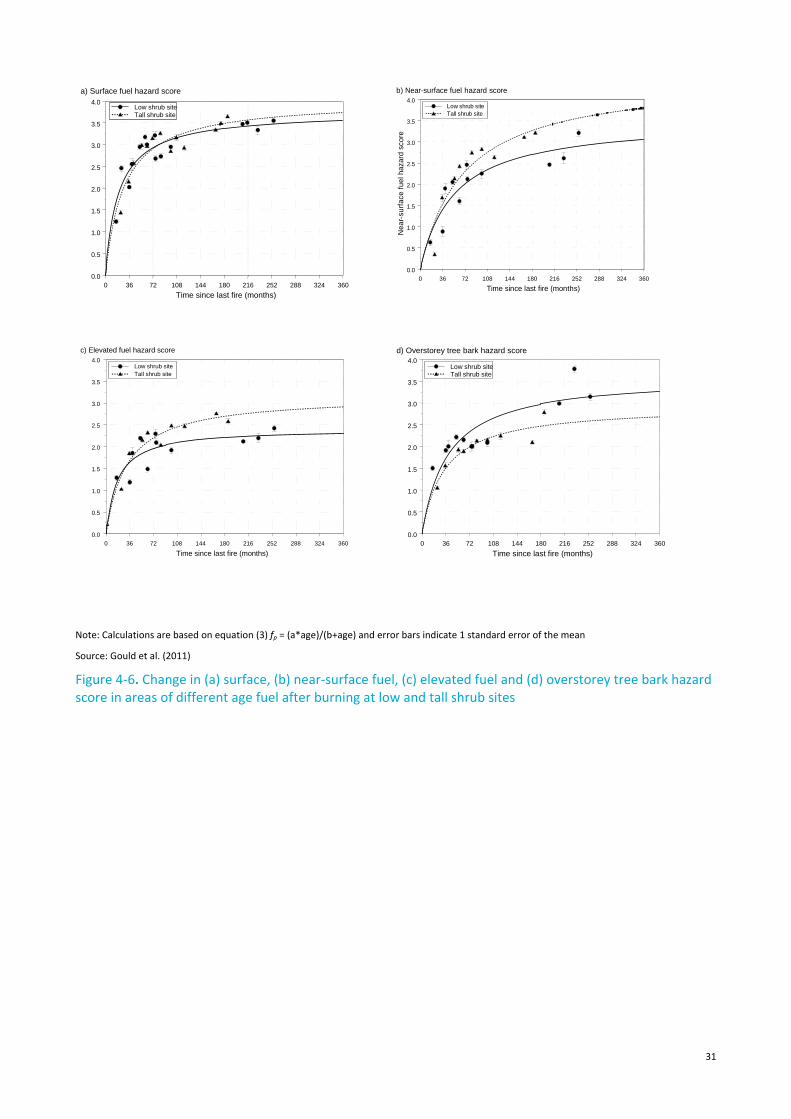
31
Note: Calculations are based on equation (3) fp = (a*age)/(b+age) and error bars indicate 1 standard error of the mean
Source: Gould et al. (2011)
Figure 4‐6. Change in (a) surface, (b) near‐surface fuel, (c) elevated fuel and (d) overstorey tree bark hazard score in areas of different age fuel after burning at low and tall shrub sites
0 36 72 108 144 180 216 252 288 324 360
Time since last fire (months)
0.0
0.5
1.0
1.5
2.0
2.5
3.0
3.5
4.0
Nea
r-su
rfac
e fu
el h
azar
d sc
ore
b) Near-surface fuel hazard score
Low shrub siteTall shrub site
0 36 72 108 144 180 216 252 288 324 360
Time since last fire (months)
0.0
0.5
1.0
1.5
2.0
2.5
3.0
3.5
4.0
d) Overstorey tree bark hazard score
Low shrub siteTall shrub site
0 36 72 108 144 180 216 252 288 324 360
Time since last fire (months)
0.0
0.5
1.0
1.5
2.0
2.5
3.0
3.5
4.0
c) Elevated fuel hazard score Low shrub site Tall shrub site
0 36 72 108 144 180 216 252 288 324 360
Time since last fire (months)
0.0
0.5
1.0
1.5
2.0
2.5
3.0
3.5
4.0
a) Surface fuel hazard score
Low shrub site Tall shrub site
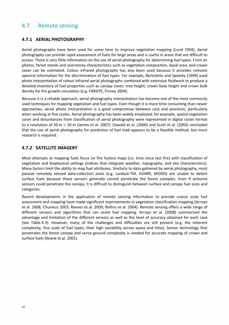
32
4.7 Remote sensing
4.7.1 AERIAL PHOTOGRAPHY
Aerial photographs have been used for some time to improve vegetation mapping (Lund 1969). Aerial photography can provide rapid assessment of fuels for large areas and is useful in areas that are difficult to access. There is very little information on the use of aerial photography for determining fuel types. From air photos, forest stands and overstorey characteristics such as vegetation composition, basal area, and crown cover can be estimated. Colour infrared photography has also been used because it provides relevant spectral information for the discrimination of fuel types. For example, Bertolette and Spotsky (1999) used photo interpretation of colour infrared aerial photographs combined with extensive fieldwork to produce a detailed inventory of fuel properties such as canopy cover, tree height, crown base height and crown bulk density for fire growth simulation (e.g. FARSITE, Finney 2004).
Because it is a reliable approach, aerial photography interpretation has become one of the most commonly used techniques for mapping vegetation and fuel types. Even though it is more time consuming than newer approaches, aerial photo interpretation is a good compromise between cost and precision, particularly when working at fine scales. Aerial photography has been widely employed; for example, spatial vegetation cover and disturbances from classification of aerial photography were represented in digital raster format
to a resolution of 50 m 50 m (James et al. 2007). Oswald et al. (2000) and Scott et al. (2002) concluded that the use of aerial photography for prediction of fuel load appears to be a feasible method, but more research is required.
4.7.2 SATELLITE IMAGERY
Most attempts at mapping fuels focus on fire history maps (i.e. time since last fire) with classification of vegetation and biophysical settings (indices that integrate weather, topography, and site characteristics). Many factors limit the ability to map fuel attributes. Similarly to data gathered by aerial photography, most passive remotely sensed data‐collection tools (e.g. Landsat‐TM, AVHRR, MODIS) are unable to detect surface fuels because these sensors generally cannot penetrate the forest canopies. Even if airborne sensors could penetrate the canopy, it is difficult to distinguish between surface and canopy fuel sizes and categories.
Recent developments in the application of remote sensing information to provide coarse scale fuel assessment and mapping have made significant improvements in vegetation classification mapping (Arroyo et al. 2008; Chuvieco 2003; Reeves et al. 2009; Rollins et al. 2004). Remote sensing offers a wide range of different sensors and algorithms that can assist fuel mapping. Arroyo et al. (2008) summarised the advantage and limitation of the different sensors as well as the level of accuracy obtained for each case (see Table 4‐3). However, many of the challenges and difficulties are still present (e.g. the inherent complexity, fine scale of fuel types, their high variability across space and time), Sensor technology that penetrates the forest canopy and sense ground complexity is needed for accurate mapping of crown and surface fuels (Keane et al. 2001).
33
Table 4‐3. Advantages, disadvantages, techniques and scales of different remote sensing data applied to fuel mapping
Sensor Methodological approach
Advantages Disadvantages Scale
AVHRR, MODIS Maximum likelihood classification algorithm; spectral mixture analysis
Possibility of updating the information on a daily basis
Coarse resolution of the sensor limits its utility to regional and global scales
500 m – 5 km
Landsat, SPOT, ASTER
Supervised classification of multi‐temporal imagery, ancillary data and texture
Easy access and reasonable cost
Cannot sense under the canopy, limited spatial resolution
30–500 m
QuickBird, IKONOS
Object based classification; maximum likelihood classification
Detailed information; adequate for wildland–urban interface
Expensive, time consuming, it requires expert users and specific software
5–30 m
AVIRIS, DAIS7915, HyMap
Spectral mixture analysis; supervised classifications
Adapted to fuel characteristics; biophysical component mapping, better adapted to temporal changes,
Complicated data processing; restrictive area cover; higher cost per are unit than other sensors
5–30 m
RadidEye Multi‐spectral imager acquires data in 5 different spectral bands
1–2 day revisit coverage, application in forestry, vegetation classification, damage assessment, low cost per unit area
Requires innovation in data handling, storage and backup
6.5 m
LiDAR (various airborne small footprint laser scanner systems)
Regression analysis, tree segmentation, vertical profiles, development of algorithms
Lower cost than manual inventory, direct height measurement; some information of sub‐canopy structures
Complicate data processing; restrictive area cover; higher cost per unit area than other sensors
< 5 m
RADAR (microwave sensors)
Semi‐empirical algorithms, over Synthetic Aperture Radar (SAR) imagery to estimate biomass distribution and fuel load parameter
Cheaper to acquire,allows large areas to be analysed
Not capable of providing three‐dimensional information about vegetation structure, not operative on steep slopes
< 5 m
Combined methods
ASTER+ gradient modelling; LiDAR+ multispectral data; LiDAR+hyerspectral data
Integration of information; rapid assessment of fire fuel conditions at large scale
Requires operators to have expertise in different techniques
< 30 m
ASTER = Advanced Spaceborne Thermal Emission And Reflection Radiometer; AVHRR = Advanced Very High Resolution Radiometer; AVIRIS = Airborne Visible and Infrared Imaging Spectrometer; DAIS7915 = Digital Airborne Imaging Spectrometer; HyMap = Airborne Hyperspectral Imaging Sensor; IKONOS = the first commercial high‐resolution satellite; LiDAR = Light Detection and Ranging; MODIS = Moderate‐Resolution Imaging Spectroradiometer; QuickBird = high‐resolution commercial earth observation satellite; SPOT = Le Système l’Observation de la Terre
Sources: Keane et al. (2001); Lanorte and Lasponara (2007); Melesse et al. (2007); Arroyo et al. (2008)
34
A study in New South Wales investigated the feasibility of estimating fuel load and other fuel attributes in forest areas using remote sensing technology (RFS 2007). The project developed a ground survey methodology for measurement and assessment of fuel loads, to provide a benchmark against which the remote sensing would seek to identify variations in fuel load. This methodology used destructive sampling and visual assessment of fuel hazard and percentage cover for 130 sites in the 12 800 hectare study area. Data sets from four satellite‐borne sensors (SPOT2, SPOT5, LandSat5 TM and ASTER) and three airborne sensors (Daedalus, HyMap, and LiDAR) were collected for the same study area, providing a comprehensive array of information about the study site. Analysis of the ground survey data showed only a weak relationship between visual and destructive sampling methods. This may suggest that visual fuel assessment methods need improvement, or destructive sampling techniques were insufficient to cover the variation within plots of 20 m radius. In particular, the ground survey data contained wide variability in destructive samples for each layer, suggesting that the fuels in the field were highly variable at the scale being measured.
None of the remote sensing systems used in this study are able to provide accurate broad‐scale maps depicting a continuous scale of combined surface, near‐surface and elevated fuels. However, operationally useful, broad‐scale maps depicting categorised fuel load estimates derived from Normalised Difference Vegetation Index (NDVI) analysis can be generated using airborne hyperspectral and SPOT5 and SPOT2 satellite‐borne optical sensors, and LIDAR can spatially map elevated fuels. There are limitations to the range of vegetation types that could be accurately assessed by satellite and airborne optical sensing, driven largely by the nature of vegetation canopy cover and density. The Rural Fire Service study confirmed that with increasing canopy cover and density, optical remote sensing methods have declining ability to accurately measure forest fuel loads, due to the effect of the canopy optically obscuring other live and dead vegetation beneath it.
Grassland is the most common fuel type in Australia. Nearly 75% of the country is grassland of one species or another, with half of that made up of areas used for livestock grazing (Cheney and Sullivan 2008). The dead moisture content and degree of curing of grass fuel determines the vulnerability of grasses to propagate and carry fire. Grassland curing is the progressive senescence and drying out of a grass, which is defined as the percentage of dead material in the grass sward. Together with air temperature (°C), relative humidity (%) and wind speed (km h‐1), the degree of curing is an input into the grassland fire danger meter and fire spread models (Cheney et al. 1998), which are used to provide regional fire danger warnings in southern Australia, and to gain reliable information for purposes of fire control and prescribed burning in northern Australia.
Satellite remote sensing systems can monitor grass curing using a combination of specific wavelengths sensitive to certain biophysical changes, such as cellular structure, and changing levels of chlorophyll content, cellulose content and water content. Since the 1980s, National Oceanic and Atmospheric Administration (NOAA) Advanced Very High Resolution Radiometer (AVHRR) data have been used operationally to derive satellite‐based maps of grassland curing across southeastern Australia, via the NDVI. These curing maps are based on an algorithm developed initially by the CSIRO and the Victorian Country Fire Authority (CFA) (Paltridge and Barber 1988; Barber 1990). This algorithm; however, was based on curing data collected from improved pastures in Victoria and may not be appropriate for other grassland types (such as native grasses) or other regions. Also, these satellite measurements are complemented by in situ visual observations, which are generally sparse over both space and time, and their accuracy may vary greatly depending on observer experience. The greatest limitation of these ground measurements is the spatial density and temporal frequency achievable, which can affect time‐critical fire hazard warnings and the availability of data for predicting fire behaviour. Grasses can senesce rapidly during dry periods. Satellite spectral indices have been used to predict the degree of curing in Australia (Barber 1990; Newnham et al. 2011; Paltridge and Barber 1988). Cloud cover, tree cover and density and coarse scale (e.g. MODIS 500 m spatial resolution) are some of the limitations in estimating grass curing at the regional and local level for some of the fire agencies (David Nichols, Victorian Country Fire Authority, pers. comm. 2012).
Recent research by Newnham et al. (2007) and Martin (2009) provided improvements to current operational satellite remote sensing methods for the assessment of grassland curing across Australia.
35
Rather than deriving a satellite algorithm from in situ visual observations carried out in Victorian improved pastures alone, this research has used a more accurate technique, Levy rod sampling, at 29 field sites of different soil and grass types, and in different climate zones. Using MODIS satellite imagery to capture these grasslands, the results from these studies have confirmed NDVI to be the best performing index for curing prediction across all Australian sites and bioclimatic regions.
4.7.3 LIDAR
The availability of airborne LiDAR (light detection and ranging) has seen a substantial increase over the recent years (Brown, et al. 2011; Goodwin et al. 2009; Reutebuch et al. 2005). LiDAR has the potential to provide more detailed information on canopy structure because it effectively adds a third dimension‐range to the data. LiDAR technology provides new sensors for measuring and monitoring biospatial data across the landscape. The basis of LIDAR is the ability to directly measure the three‐dimensional (3D) structure (i.e. terrain, vegetation, and infrastructure) of imaged areas and to separate biospatial data (measurements of terrain surface). This allows LiDAR to provide both a useful map of the position of the ground surface along with an indication of how the foliage and stems are arranged vertically above the ground (Jupp et al. 2005).
Research found that whilst surface and near‐surface fuels were difficult to distinguish using airborne LiDAR data, there was reasonable correlation between elevated fuel components and LiDAR information. Power (2006) and Turner (2007) found that understorey characteristics appeared to be correlated with topographic features. However, in order to achieve a broader landscape approach to fuel stratification, there is a need to integrate topographic feathers (i.e. slope and aspect) with LiDAR data through a rule‐based approach, using spatial segmentation and aggregation for better delineation of understorey structure (Brown et al. 2011).
Several major fuel types and components became readily observable using LiDAR data for fuel stratification. The use of LiDAR in conjunction with aerial photography simplified and improved the stratification. The limiting application of LiDAR data is that it represents near top height for any vegetation for the first return signal, which does not lend itself to accurate understorey height and density (Brown et al. 2011).
4.7.4 LIDAR AND WILDLAND–URBAN FUELS
Wildland–urban interface (WUI) areas are places where structures and other human development meet or mix with the bush and/or rural environment. WUI environments are structurally and geometrically complex, and vary widely due to differences in building density, height, and materials, and vegetation characteristics such as height, and vegetated cover. Information on WUI fuel characteristics is critical for effective emergency response. Currently there is limited information characterising WUI fuels. WUIs create an environment in which bushfires can move easily between structures and vegetation fuels. Their expansion has thus increased the likelihood that bushfire will threaten structures and people. The main objective in characterising WUI fuels is to provide standardised information to assist home owners, fire managers and fire‐fighters with a view to develop specific actions for bushfire prevention, to create public awareness of bushfire risk and assess suppression difficulty due to urbanisation. Figure 4‐7 illustrates a set of processes for characterising WUI fuel, which will be incorporated into the Australian Fuel Classification.
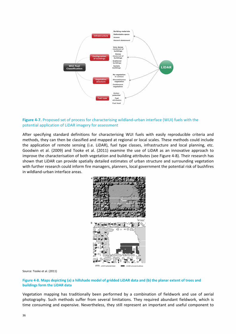
36
Figure 4‐7. Proposed set of process for characterising wildland‐urban interface (WUI) fuels with the potential application of LiDAR imagery for assessment
After specifying standard definitions for characterising WUI fuels with easily reproducible criteria and methods, they can then be classified and mapped at regional or local scales. These methods could include the application of remote sensing (i.e. LiDAR), fuel type classes, infrastructure and local planning, etc. Goodwin et al. (2009) and Tooke et al. (2011) examine the use of LiDAR as an innovative approach to improve the characterisation of both vegetation and building attributes (see Figure 4‐8). Their research has shown that LiDAR can provide spatially detailed estimates of urban structure and surrounding vegetation with further research could inform fire managers, planners, local government the potential risk of bushfires in wildland‐urban interface areas.
Source: Tooke et al. (2011)
Figure 4‐8. Maps depicting (a) a hillshade model of gridded LiDAR data and (b) the planar extent of trees and buildings form the LiDAR data
Vegetation mapping has traditionally been performed by a combination of fieldwork and use of aerial photography. Such methods suffer from several limitations. They required abundant fieldwork, which is time consuming and expensive. Nevertheless, they still represent an important and useful component to

37
the remote sensing approach. Fieldwork in conjunction with aerial photography provides the field reference datasets necessary to validate maps created by remote‐sensed data products. Remote sensing methods offer several advantages, and when incorporated with field observation, the results are markedly improved. Airborne sensors can offer cost‐effective ways to access bushfire risk in real‐time with wider spatial and regular temporal coverage (e.g. grassland curing). However, the data are processed digitally, and analysis may be complex, expensive or impossible with visual products. Several shortcomings have limited the use of remote sensed data for fuel assessment. Optical satellite data and aerial photographs are limited to observing the horizontal fuel distribution and are constrained by their inability to reveal understorey characteristic and fine scale fuel attributes. With the development of new improved sensors (e.g. airborne and ground LiDAR) and techniques (e.g. object‐oriented image analysis, improved algorithms) fuel‐mapping tasks can be considerably improved. Review and research should continue into the application of remote sensors application for bushfire fuel classification, focusing on integration of mapping techniques, sensor data, and field validation In addition, ecosystems simulation modelling can play an important role in quantifying those gradients responsible for fuel distributions to aid in image classification for bushfire fuel mapping.
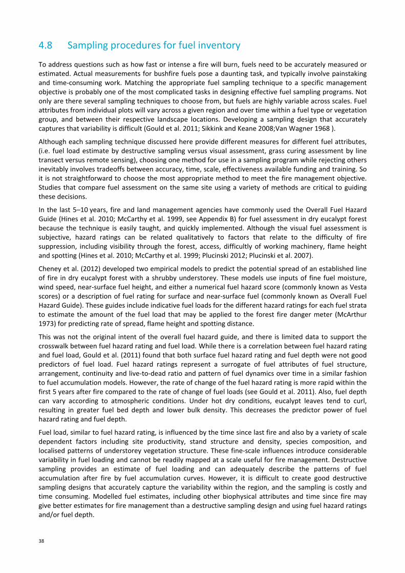
38
4.8 Sampling procedures for fuel inventory
To address questions such as how fast or intense a fire will burn, fuels need to be accurately measured or estimated. Actual measurements for bushfire fuels pose a daunting task, and typically involve painstaking and time‐consuming work. Matching the appropriate fuel sampling technique to a specific management objective is probably one of the most complicated tasks in designing effective fuel sampling programs. Not only are there several sampling techniques to choose from, but fuels are highly variable across scales. Fuel attributes from individual plots will vary across a given region and over time within a fuel type or vegetation group, and between their respective landscape locations. Developing a sampling design that accurately captures that variability is difficult (Gould et al. 2011; Sikkink and Keane 2008;Van Wagner 1968 ).
Although each sampling technique discussed here provide different measures for different fuel attributes, (i.e. fuel load estimate by destructive sampling versus visual assessment, grass curing assessment by line transect versus remote sensing), choosing one method for use in a sampling program while rejecting others inevitably involves tradeoffs between accuracy, time, scale, effectiveness available funding and training. So it is not straightforward to choose the most appropriate method to meet the fire management objective. Studies that compare fuel assessment on the same site using a variety of methods are critical to guiding these decisions.
In the last 5–10 years, fire and land management agencies have commonly used the Overall Fuel Hazard Guide (Hines et al. 2010; McCarthy et al. 1999, see Appendix B) for fuel assessment in dry eucalypt forest because the technique is easily taught, and quickly implemented. Although the visual fuel assessment is subjective, hazard ratings can be related qualitatively to factors that relate to the difficulty of fire suppression, including visibility through the forest, access, difficultly of working machinery, flame height and spotting (Hines et al. 2010; McCarthy et al. 1999; Plucinski 2012; Plucinski et al. 2007).
Cheney et al. (2012) developed two empirical models to predict the potential spread of an established line of fire in dry eucalypt forest with a shrubby understorey. These models use inputs of fine fuel moisture, wind speed, near‐surface fuel height, and either a numerical fuel hazard score (commonly known as Vesta scores) or a description of fuel rating for surface and near‐surface fuel (commonly known as Overall Fuel Hazard Guide). These guides include indicative fuel loads for the different hazard ratings for each fuel strata to estimate the amount of the fuel load that may be applied to the forest fire danger meter (McArthur 1973) for predicting rate of spread, flame height and spotting distance.
This was not the original intent of the overall fuel hazard guide, and there is limited data to support the crosswalk between fuel hazard rating and fuel load. While there is a correlation between fuel hazard rating and fuel load, Gould et al. (2011) found that both surface fuel hazard rating and fuel depth were not good predictors of fuel load. Fuel hazard ratings represent a surrogate of fuel attributes of fuel structure, arrangement, continuity and live‐to‐dead ratio and pattern of fuel dynamics over time in a similar fashion to fuel accumulation models. However, the rate of change of the fuel hazard rating is more rapid within the first 5 years after fire compared to the rate of change of fuel loads (see Gould et al. 2011). Also, fuel depth can vary according to atmospheric conditions. Under hot dry conditions, eucalypt leaves tend to curl, resulting in greater fuel bed depth and lower bulk density. This decreases the predictor power of fuel hazard rating and fuel depth.
Fuel load, similar to fuel hazard rating, is influenced by the time since last fire and also by a variety of scale dependent factors including site productivity, stand structure and density, species composition, and localised patterns of understorey vegetation structure. These fine‐scale influences introduce considerable variability in fuel loading and cannot be readily mapped at a scale useful for fire management. Destructive sampling provides an estimate of fuel loading and can adequately describe the patterns of fuel accumulation after fire by fuel accumulation curves. However, it is difficult to create good destructive sampling designs that accurately capture the variability within the region, and the sampling is costly and time consuming. Modelled fuel estimates, including other biophysical attributes and time since fire may give better estimates for fire management than a destructive sampling design and using fuel hazard ratings and/or fuel depth.
39
Sampling procedures are useful to provide estimates of fuel attributes needed for fire behaviour prediction and for planning prescribed burns, risk monitoring and treatment, and other fire management activities. The procedures and sampling design will depend on the accuracy required, practicality, and efficiency over the study area. Recommended sample procedures for different fuel types (presented in Table 4‐4) can be widely applied with minimum training and cost. These procedures are based on homogenous fuel cover, and if better estimates are required then a greater number of samples are needed. The recommended fuel sampling procedures presented here are a minimum guideline. Depending on the needs and levels of accuracy required by users, more or fewer samples may be required. Fire managers may require additional information; for example, if developing fuel dynamic models for a specific region then a more robust sampling design is required, compared to knowing the estimate of coarse woody debris for suppression mop‐up planning. With a more robust sampling design with increasing number of samples, you will gain increased confidence with the data, and this is often associated with increasing costs.
It is also important for any fuel assessment methodology to address the various needs and levels of accuracy required by each user. Table 4‐5 provides a listing of fuel sampling methods and an associated ranking of accuracy and cost (Gould et al. 2012). While some methodologies may be widely accepted throughout the scientific literature because of their high levels of accuracy, these are often time consuming and the level of accuracy obtained may not be required by fire management applications. For this reason, a less time consuming and robust method may be more appropriate. For example, for the purposes of research, transect lengths upwards of 500 m together with replicates of at least 20 may be required to ensure an acceptable level of precision for estimating the load of dead and downed logs within a forested area (Miehs et al. 2009). But this level of accuracy may not be needed by a fire manager wishing to estimate smoke production or mop‐up requirements. Instead, an average woody fuel load determined by fuel type may be adequate. Fuel assessment methodology should also take into account the inherent sensitivity of fire behaviour models to each particular fuel input parameter (or attribute) under varying fire behaviour conditions. As another example, a fire manager wishing to plan a prescribed burn under low–mild burning conditions may have little need for a highly accurate estimate of the quantity of fuel in the forest canopy. However, given that the use of a fire behaviour model that is very sensitive to the litter load, a sampling method will require a methodology that provides a timely, but accurate measure of surface litter load. While more information is needed to define the sensitivity of fire behaviour models to each fuel parameter and the degree of accuracy provided by each fuel assessment technique, fuel assessment protocols should consider the various uses and levels of accuracy required by users.
Each fuel assessment technique should accurately and consistently measure fuel characteristics across a wide variety of components. In addition, the techniques must be:
easily taught to field crew
quickly implemented
scalable so that any sampling unit can be measured and fuel components are measured at an appropriate spatial scale
of known accuracy, so estimates can be relied upon for the purpose they are collected
repeatable so that estimates can be measured at a precision that is required for fire management applications.
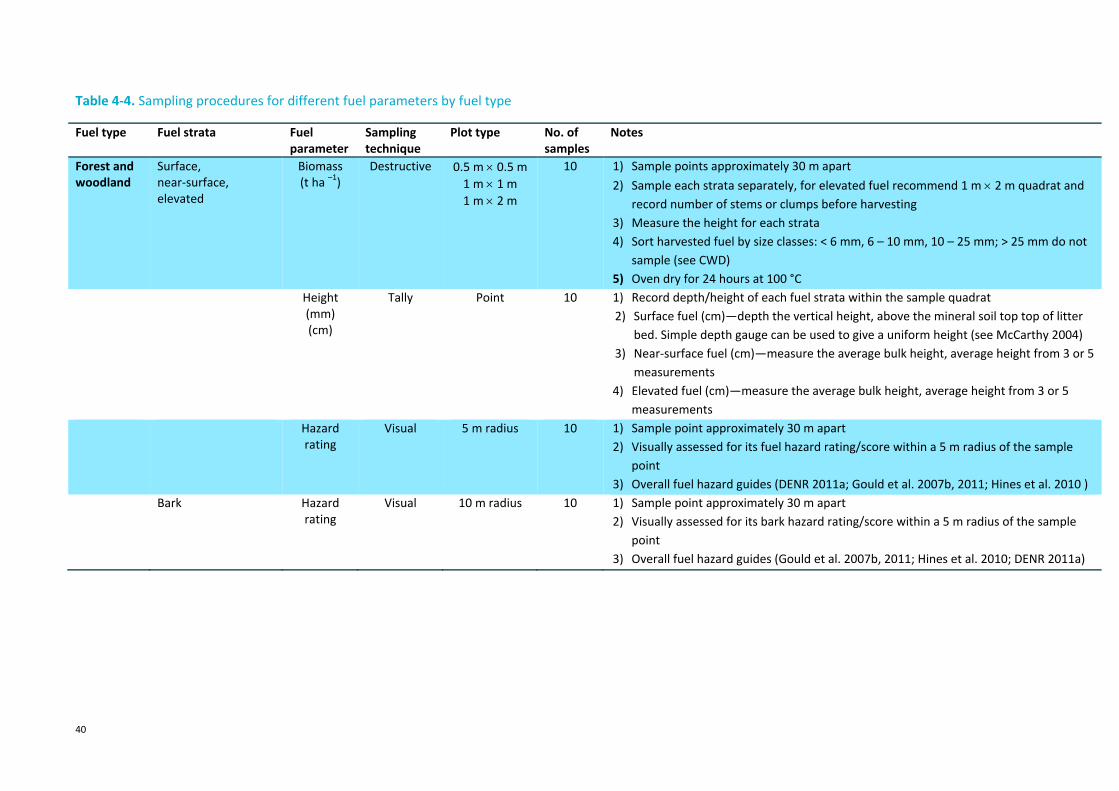
40
Table 4‐4. Sampling procedures for different fuel parameters by fuel type
Fuel type Fuel strata Fuel parameter
Sampling technique
Plot type No. of samples
Notes
Forest and woodland
Surface, near‐surface, elevated
Biomass (t ha –1)
Destructive 0.5 m 0.5 m
1 m 1 m
1 m 2 m
10 1) Sample points approximately 30 m apart
2) Sample each strata separately, for elevated fuel recommend 1 m 2 m quadrat and
record number of stems or clumps before harvesting
3) Measure the height for each strata
4) Sort harvested fuel by size classes: < 6 mm, 6 – 10 mm, 10 – 25 mm; > 25 mm do not
sample (see CWD)
5) Oven dry for 24 hours at 100 °C
Height(mm) (cm)
Tally Point 10 1) Record depth/height of each fuel strata within the sample quadrat
2) Surface fuel (cm)—depth the vertical height, above the mineral soil top top of litter
bed. Simple depth gauge can be used to give a uniform height (see McCarthy 2004)
3) Near‐surface fuel (cm)—measure the average bulk height, average height from 3 or 5
measurements
4) Elevated fuel (cm)—measure the average bulk height, average height from 3 or 5
measurements
Hazard rating
Visual 5 m radius 10 1) Sample point approximately 30 m apart
2) Visually assessed for its fuel hazard rating/score within a 5 m radius of the sample
point
3) Overall fuel hazard guides (DENR 2011a; Gould et al. 2007b, 2011; Hines et al. 2010 )
Bark Hazard rating
Visual 10 m radius 10 1) Sample point approximately 30 m apart
2) Visually assessed for its bark hazard rating/score within a 5 m radius of the sample
point
3) Overall fuel hazard guides (Gould et al. 2007b, 2011; Hines et al. 2010; DENR 2011a)
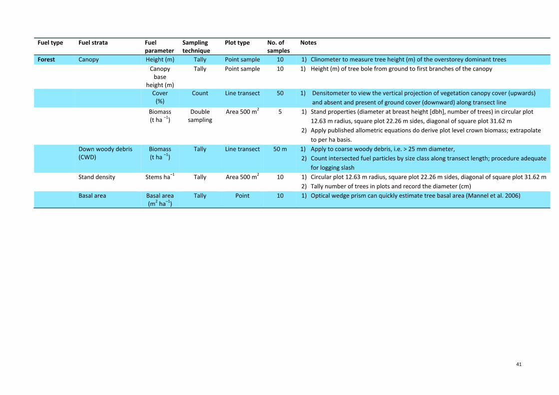
41
Fuel type Fuel strata Fuel parameter
Sampling technique
Plot type No. of samples
Notes
Forest Canopy Height (m) Tally Point sample 10 1) Clinometer to measure tree height (m) of the overstorey dominant trees
Canopy base
height (m)
Tally Point sample 10 1) Height (m) of tree bole from ground to first branches of the canopy
Cover(%)
Count Line transect 50 1) Densitometer to view the vertical projection of vegetation canopy cover (upwards)
and absent and present of ground cover (downward) along transect line
Biomass(t ha –1)
Double sampling
Area 500 m2 5 1) Stand properties (diameter at breast height [dbh], number of trees) in circular plot
12.63 m radius, square plot 22.26 m sides, diagonal of square plot 31.62 m
2) Apply published allometric equations do derive plot level crown biomass; extrapolate
to per ha basis.
Down woody debris (CWD)
Biomass (t ha –1)
Tally Line transect 50 m 1) Apply to coarse woody debris, i.e. > 25 mm diameter,
2) Count intersected fuel particles by size class along transect length; procedure adequate
for logging slash
Stand density Stems ha–1 Tally Area 500 m2 10 1) Circular plot 12.63 m radius, square plot 22.26 m sides, diagonal of square plot 31.62 m
2) Tally number of trees in plots and record the diameter (cm)
Basal area Basal area(m2 ha–1)
Tally Point 10 1) Optical wedge prism can quickly estimate tree basal area (Mannel et al. 2006)
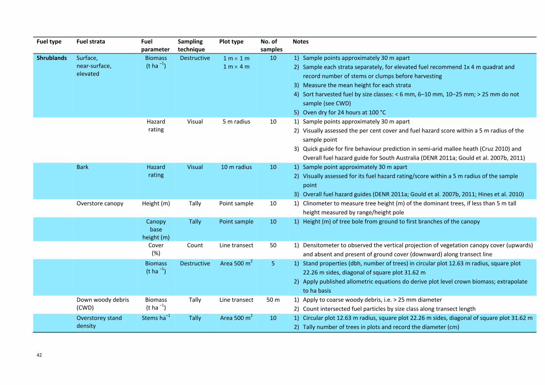
42
Fuel type Fuel strata Fuel parameter
Sampling technique
Plot type No. of samples
Notes
Shrublands Surface, near‐surface, elevated
Biomass (t ha –1)
Destructive 1 m 1 m
1 m 4 m
10 1) Sample points approximately 30 m apart
2) Sample each strata separately, for elevated fuel recommend 1x 4 m quadrat and
record number of stems or clumps before harvesting
3) Measure the mean height for each strata
4) Sort harvested fuel by size classes: < 6 mm, 6–10 mm, 10–25 mm; > 25 mm do not
sample (see CWD)
5) Oven dry for 24 hours at 100 °C
Hazard rating
Visual 5 m radius 10 1) Sample points approximately 30 m apart
2) Visually assessed the per cent cover and fuel hazard score within a 5 m radius of the
sample point
3) Quick guide for fire behaviour prediction in semi‐arid mallee heath (Cruz 2010) and
Overall fuel hazard guide for South Australia (DENR 2011a; Gould et al. 2007b, 2011)
Bark Hazard rating
Visual 10 m radius 10 1) Sample point approximately 30 m apart
2) Visually assessed for its fuel hazard rating/score within a 5 m radius of the sample
point
3) Overall fuel hazard guides (DENR 2011a; Gould et al. 2007b, 2011; Hines et al. 2010)
Overstore canopy Height (m) Tally Point sample 10 1) Clinometer to measure tree height (m) of the dominant trees, if less than 5 m tall
height measured by range/height pole
Canopy base
height (m)
Tally Point sample 10 1) Height (m) of tree bole from ground to first branches of the canopy
Cover(%)
Count Line transect 50 1) Densitometer to observed the vertical projection of vegetation canopy cover (upwards)
and absent and present of ground cover (downward) along transect line
Biomass(t ha –1)
Destructive Area 500 m2 5 1) Stand properties (dbh, number of trees) in circular plot 12.63 m radius, square plot
22.26 m sides, diagonal of square plot 31.62 m
2) Apply published allometric equations do derive plot level crown biomass; extrapolate
to ha basis
Down woody debris (CWD)
Biomass (t ha –1)
Tally Line transect 50 m 1) Apply to coarse woody debris, i.e. > 25 mm diameter
2) Count intersected fuel particles by size class along transect length
Overstorey stand density
Stems ha–1 Tally Area 500 m2 10 1) Circular plot 12.63 m radius, square plot 22.26 m sides, diagonal of square plot 31.62 m
2) Tally number of trees in plots and record the diameter (cm)
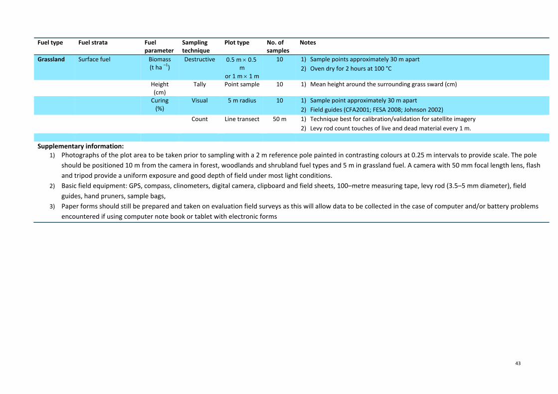
43
Fuel type Fuel strata Fuel parameter
Sampling technique
Plot type No. of samples
Notes
Grassland Surface fuel Biomass (t ha –1)
Destructive 0.5 m 0.5 m
or 1 m 1 m
10 1) Sample points approximately 30 m apart
2) Oven dry for 2 hours at 100 °C
Height (cm)
Tally Point sample 10 1) Mean height around the surrounding grass sward (cm)
Curing(%)
Visual 5 m radius 10 1) Sample point approximately 30 m apart
2) Field guides (CFA2001; FESA 2008; Johnson 2002)
Count Line transect 50 m 1) Technique best for calibration/validation for satellite imagery
2) Levy rod count touches of live and dead material every 1 m.
Supplementary information: 1) Photographs of the plot area to be taken prior to sampling with a 2 m reference pole painted in contrasting colours at 0.25 m intervals to provide scale. The pole
should be positioned 10 m from the camera in forest, woodlands and shrubland fuel types and 5 m in grassland fuel. A camera with 50 mm focal length lens, flash
and tripod provide a uniform exposure and good depth of field under most light conditions.
2) Basic field equipment: GPS, compass, clinometers, digital camera, clipboard and field sheets, 100–metre measuring tape, levy rod (3.5–5 mm diameter), field
guides, hand pruners, sample bags,
3) Paper forms should still be prepared and taken on evaluation field surveys as this will allow data to be collected in the case of computer and/or battery problems
encountered if using computer note book or tablet with electronic forms
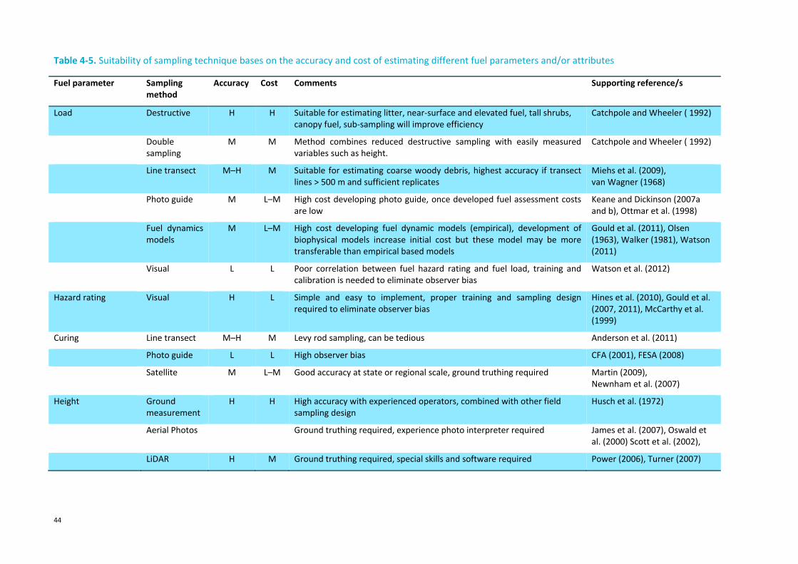
44
Table 4‐5. Suitability of sampling technique bases on the accuracy and cost of estimating different fuel parameters and/or attributes
Fuel parameter Sampling method
Accuracy Cost Comments Supporting reference/s
Load Destructive H H Suitable for estimating litter, near‐surface and elevated fuel, tall shrubs, canopy fuel, sub‐sampling will improve efficiency
Catchpole and Wheeler ( 1992)
Double sampling
M M Method combines reduced destructive sampling with easily measured variables such as height.
Catchpole and Wheeler ( 1992)
Line transect M–H M Suitable for estimating coarse woody debris, highest accuracy if transect lines > 500 m and sufficient replicates
Miehs et al. (2009), van Wagner (1968)
Photo guide M L–M High cost developing photo guide, once developed fuel assessment costs are low
Keane and Dickinson (2007a and b), Ottmar et al. (1998)
Fuel dynamics models
M L–M High cost developing fuel dynamic models (empirical), development of biophysical models increase initial cost but these model may be more transferable than empirical based models
Gould et al. (2011), Olsen (1963), Walker (1981), Watson (2011)
Visual L L Poor correlation between fuel hazard rating and fuel load, training and calibration is needed to eliminate observer bias
Watson et al. (2012)
Hazard rating Visual H L Simple and easy to implement, proper training and sampling design required to eliminate observer bias
Hines et al. (2010), Gould et al. (2007, 2011), McCarthy et al. (1999)
Curing Line transect M–H M Levy rod sampling, can be tedious Anderson et al. (2011)
Photo guide L L High observer bias CFA (2001), FESA (2008)
Satellite M L–M Good accuracy at state or regional scale, ground truthing required Martin (2009), Newnham et al. (2007)
Height Ground measurement
H H High accuracy with experienced operators, combined with other field sampling design
Husch et al. (1972)
Aerial Photos Ground truthing required, experience photo interpreter required James et al. (2007), Oswald et al. (2000) Scott et al. (2002),
LiDAR H M Ground truthing required, special skills and software required Power (2006), Turner (2007)
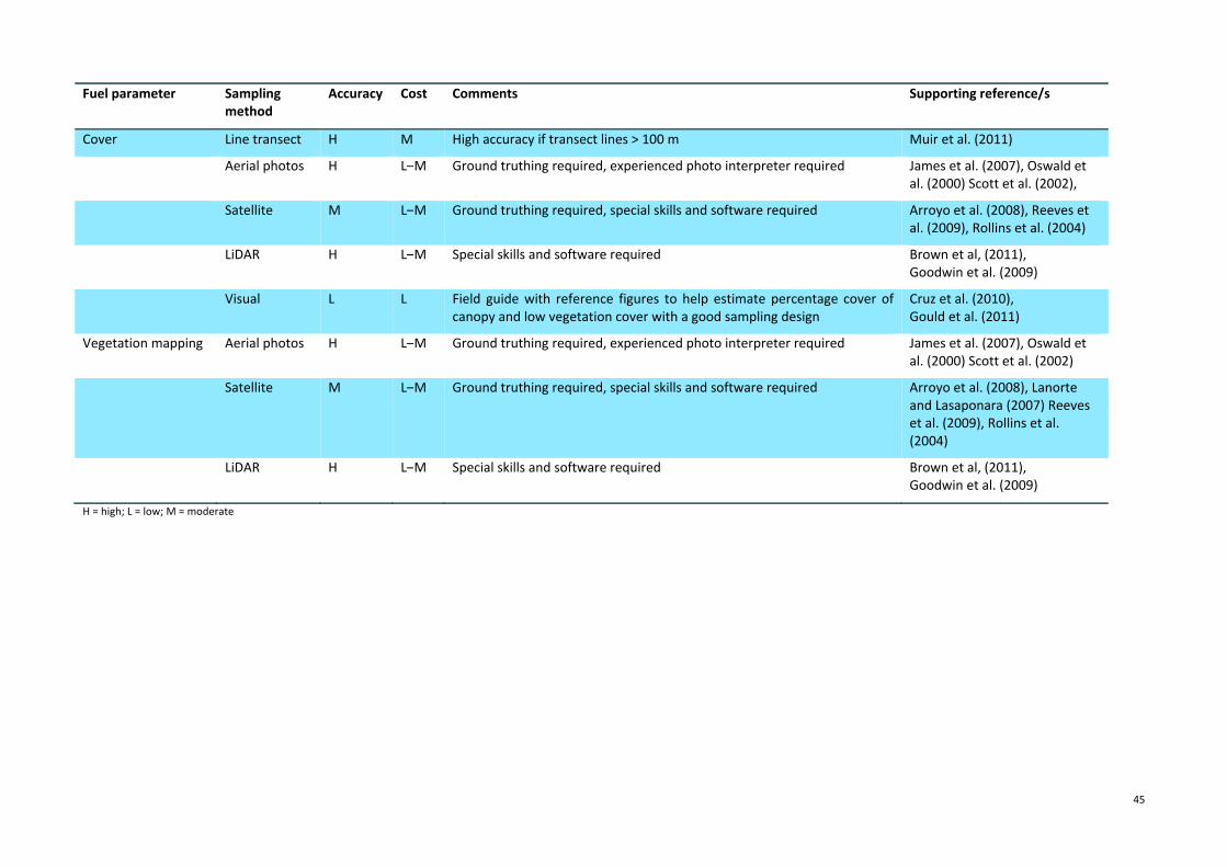
45
Fuel parameter Sampling method
Accuracy Cost Comments Supporting reference/s
Cover Line transect H M High accuracy if transect lines > 100 m Muir et al. (2011)
Aerial photos H L–M Ground truthing required, experienced photo interpreter required James et al. (2007), Oswald et al. (2000) Scott et al. (2002),
Satellite M L–M Ground truthing required, special skills and software required Arroyo et al. (2008), Reeves et al. (2009), Rollins et al. (2004)
LiDAR H L–M Special skills and software required Brown et al, (2011), Goodwin et al. (2009)
Visual L L Field guide with reference figures to help estimate percentage cover of canopy and low vegetation cover with a good sampling design
Cruz et al. (2010), Gould et al. (2011)
Vegetation mapping Aerial photos H L–M Ground truthing required, experienced photo interpreter required James et al. (2007), Oswald et al. (2000) Scott et al. (2002)
Satellite M L–M Ground truthing required, special skills and software required Arroyo et al. (2008), Lanorte and Lasaponara (2007) Reeves et al. (2009), Rollins et al. (2004)
LiDAR H L–M Special skills and software required Brown et al, (2011),Goodwin et al. (2009)
H = high; L = low; M = moderate
46
5 References
Anderson, HE 1982, Aids to determining fuel models for estimating fire behaviour, General Technical Report INT‐122, Department of Agriculture Forest Service, Intermountain Forest and Range Experiment Station, Ogden, Utah.
Anderson, S, Anderson, W, Hines, F & Fountain, A 2005, Determination of field sampling methods for the assessment of curing levels in grasslands, project A1.4 report, Bushfire Cooperative Research Centre, Melbourne.
Anderson, SAJ, Anderson, WR, Hollis, JJ & Botha, EJ 2011, ‘A simple method for field‐based grassland curing assessment’, International Journal of Wildland Fire, vol. 20, pp. 804–814.
Andrews, PL & Queen, LP 2001, ‘Fire modelling and information system technology’, International Journal of Wildland Fire, vol. 10, pp. 343–353.
Ardilly, P & Tillé, Y 2006, Sampling methods: exercise and solutions, Springer, New York.
Arroyo, LA, Pascual, C & Manzanera, JA 2008, ‘Fire models and methods to map fuel types: the role of remote sensing’, Forest Ecology and Management, vol. 256, pp. 1239–1252.
Australasian Fire and Emergency Services Authorities Council (AFAC) 2012, Bushfire glossary, AFAC, East Melbourne, viewed 12 January 2012, <http://knowledgeweb.afac.com.au/data/documents/AFAC_Bushfire_Glossary_ Indexed_2012.pdf>.
Barber, J 1990, Monitoring the curing of grassland fuels in Victoria, Australia with sensors in satellites and aircraft: a Country Fire Authority study in remote sensing, CFA, Melbourne.
Bell, G, Kerr, A, McNickle, D & Woollons, R 1996, ‘Accuracy of the line intersect method of post‐logging sampling under orientation bias’, Forest Ecology and Management, vol. 84, pp. 23–28.
Bertolette, DR & Spotskey, DB 1999, ‘Fuel model and forest type mapping for FARSITE’, the Joint Fire Science Conference and Workshop, University of Idaho and International Association of Wildland Fire, Boise, Idaho, June 15‐17, 1999.
Birk, EM & Simpson, RW 1980, ‘Steady state and the continuous input model of litter accumulation and decomposition in Australia eucalypt forest’, Ecology, vol. 61, pp. 481–485.
Brandis, K & Jacobson, C 2003, ‘Estimation of vegetative fuel load using Landsat TM imagery in New South Wales, Australia’, International Journal of Wildland Fire, vol. 12, pp. 185–194.
Brown, JK 1974, Handbook for inventorying downed woody material, General Technical Report INT‐16, USDA Forest Service, Intermountain Forest and Range Experiment Station, Ogden, Utah.
Brown, C, Scherl, T, Chylinski, T & Burns, J 2011, ‘The use of LiDAR in fuel hazard characterisation and stratification within the Sugarloaf Catchment Area’, paper presented at the AFAC & Bushfire CRC Conference Sydney, New South Wales, 29 August – 1 September 2011.
Burrows, ND 1994, ‘Experimental development of a fire management model for jarrah (Eucalyptus Marginata Donn ex Sm.) forest’, PhD thesis, Australian National University, Canberra.
Burrows, NB & McCaw, WL 1990, ‘Fuel characteristics and bushfire control in banksia low woodlands in Western Australia’, Journal of Environmental Management, vol. 34, pp. 229–236.
Burrows, NB, Ware, B & Robinson, A 1991, ‘Fire behaviour in spinifex fuels on the Gibson Desert Nature Reserve, Western Australia’, Journal of Arid Environments, vol. 20, pp. 189–204.
Catchpole, WR & Wheeler, CJ 1992, ‘Estimating plant biomass: a review of techniques’, Australian Journal of Ecology, vol. 17, pp. 121–131.
47
Cheney, NP 1990, ‘Quantifying bushfires’, Mathematical Computing and Modelling, vol. 13, pp. 9–15.
Cheney, NP, Gould, JS & Catchpole, WR 1993, ‘The influence of fuel, weather and fire shape variables on fire‐spread in grasslands’, International Journal of Wildland Fire, vol. 3, pp. 31–44.
Cheney, NP, Gould, JS & Catchpole, WR 1998, ‘Prediction of fire spread in grasslands’, International Journal of Wildland Fire, vol. 8, pp. 1–13.
Cheney, NP, Gould, JS & Hutching, PT 1990, Sampling available fuel and damage to trees retained after thinning and burning: management of eucalypt regrowth in East Gippsland, technical report no.12, Department of Conservation and Environment, Melbourne.
Cheney, NP, Gould, JS & Knight, I 1992, A prescribed burning guide for young regrowth forest of silvertop ash, research paper 16, Forestry Commission of New South Wales, West Pennant Hills, New South Wales.
Cheney, NP, Gould, JS, McCaw, WL & Anderson, WR 2012, ‘Predicting fire behaviour in dry eucalypt forest in southern Australia’, Forest Ecology and Management, vol. 280, pp. 120–131.
Cheney, P & Sullivan, A 2008, Grassfiresfuel weather and fire behaviour, 2nd edn, CSIRO Publishing, Collingwood, Victoria.
Chuvieco, E, Riano, D & van Wagtendonk, J 2003, ‘Fuel loads and fuel type mapping’, in E Chuvieco (ed.), Wildland fire danger estimation and mapping: the role of remote sensing data, World Scientific, Singapore, pp. 119–142.
Cochran, WG 1977, Sample techniques, 3rd edn, Wiley, New York.
Conroy, R 1994, Fuel management strategies in the Sydney region, New South National Parks and Wildlife Service, Hurstville, NSW.
Country Fire Authority (Victoria) 1987, Grassland curing guide, CFA Research and Planning Department, Melbourne.
Country Fire Authority (Victoria) 2001, Grassland curing guide, CFA Community Safety Department, Melbourne.
Cruz, MG 2010, Quick guide for fire behaviour prediction in semi‐arid mallee–heath, CSIRO, Canberra, & Bushfire CRC, Melbourne.
Cruz, MG, Alexander, ME & Fernandes, PM 2008, ‘Development of a model system to predict wildfire behaviour in pine plantations’, Australian Forestry, vol. 71, pp. 113–121.
Cruz, MG & Gould, J 2009, ‘National fire behaviour prediction system’, Proceedings of the Biennial Conference of the Institute of Foresters of Australia, Institute of Foresters of Australia, Caloundra, Queensland.
Cruz, MG, Matthews, S, Gould, J, Ellis, P, Henderson, M, Knight, I & Watters, J 2010, Fire dynamics in mallee‐heath: fuel, weather and fire behaviour prediction in south Australian semi‐arid shrublands, Bushfire CRC report A.10.01, CSIRO Sustainable Ecosystems, Canberra.
Cruz, M, de Mar, P & Adshead, D 2011, Radiata pine plantation fuel and fire behaviour guide, CSIRO and GDH publication for the Australian Government Department of Agriculture, Fisheries and Forestry, Canberra, ACT.
Davis, GM, Hamilton, A, Smith, A & Legg, CJ 2008, ‘Using visual obstruction to estimate heathland fuel load and structure’, International Journal of Wildland Fire, vol. 17, pp. 380–389.
Delisle, GP, Woodard, PM, Titus, SJ & Johnson, AF 1998, ‘Sample size and variability of fuel weight estimates in natural stands of lodgepole pine’, Canadian Journal of Forest Research, vol. 18, pp. 649–652.
de Mar, P & Adshead, D 2011, Blue gum plantation fuel and fire behaviour guide, GHD publication for the Australian Government Department of Agriculture, Fisheries and Forestry, Canberra, ACT.
48
Department of Environment and Heritage (DEH) 2006, Overall fuel hazard guide for South Australia, DEH, Adelaide.
Department of Environment and Natural Resources (DENR) 2011a, Overall fuel hazard guide for South Australia, 2nd edn, DENR, Adelaide.
Department of Environment and Natural Resources (DENR) 2011b, Fire policy and procedures manual, DENR, Adelaide.
DeVries, PG 1974, ‘Multi‐stage line intersect sampling’, Forest Science, vol. 20, pp. 129–133.
Fensham, RJ 1992, ‘The management implication of fine fuel dynamics in bushland surrounding Hobart, Tasmania’, Journal of Environmental Management, vol. 36, pp. 301–320.
Finney, MA 2004, FARSITE: fire area simulator—model development and evaluation, research paper RMRS‐RP‐4 revised, USDA Forest Service, Rocky Mountain Research Station, Fort Collins, Colorado.
Fire and Emergency Services Authority of Western Australia (FESA) 2007a, Visual fuel load guide for the scrub vegetation of the Swan Coastal Plain, FESA, Perth, viewed 14 August 2012, <http://www.fesa.wa.gov.au/safetyinformation/fire/bushfire/Pages/publications.aspx#5>.
Fire and Emergency Services Authority of Western Australia (FESA) 2007b, Visual fuel load guide for the Kimberley region, FESA, Perth, viewed 14 August 2012, <http://www.fesa.wa.gov.au/safetyinformation/fire/bushfire/Pages/publications.aspx#5>.
Fire and Emergency Services Authority of Western Australia (FESA) 2008, Grass curing visual guide for Western Australia, FESA, Perth, viewed 14 August 2012,<http://www.fesa.wa.gov.au/safetyinformation/fire/bushfire/Pages/publications.aspx#5>.
Fire and Emergency Services Authority of Western Australia (FESA) 2009, Visual fuel load guide for the Pilbara region, FESA, Perth, viewed 14 August 2012, <http://www.fesa.wa.gov.au/safetyinformation/fire/bushfire/Pages/publications.aspx#5>.
Fire and Emergency Services Authority of Western Australia (FESA) 2010a, Visual fuel load guide for the Goldfields region, FESA, Perth, viewed 14 August 2012, <http://www.fesa.wa.gov.au/safetyinformation/fire/bushfire/Pages/publications.aspx#5>.
Fire and Emergency Services Authority of Western Australia (FESA) 2010b, Visual fuel load guide for the Esperance Plains, FESA, Perth, viewed 14 August 2012, <http://www.fesa.wa.gov.au/safetyinformation/fire/bushfire/Pages/publications.aspx#5>.
Fire and Emergency Services Authority of Western Australia (FESA) 2010c, Visual fuel load guide for Denmark Shire, FESA, Perth, viewed 14 August 2012, <http://www.fesa.wa.gov.au/safetyinformation/fire/bushfire/Pages/publications.aspx#5>.
Fischer, WC 1981a, Photo guide for appraising downed woody fuels in Montana forest: interior ponderosa pine, ponderosa pine‐larch‐Douglas‐fir, larch‐Douglas‐ fir and interior Douglas‐fir cover types, General Technical Report INT‐97, USDA Forest Service, Intermountain Forest and Range Experimental Station, Ogden, Utah.
Fischer, WC 1981b, Photo guides for appraising downed wood fuels in Montana forests; how they were made, Research Note INT‐288, USDA Forest Service, Intermountain Forest and Range Experimental Station, Ogden, Utah.
Fox, BJ, Fox, MD & McKay, GM 1979, ‘Litter accumulation after fire in a eucalypt forest’, Australian Journal of Botany, vol. 27, pp. 157–165.
Goodwin, NR, Coops, NC, Tooke, TR, Christen, A & Voogt, JA 2009, ‘Characterizing urban surface cover and structure with airborne LiDAR technology’, Canadian Journal of Remote Sensing, vol. 35, pp. 297–309.
Gould, JS 1994, ‘Evaluation of McArthur’s control burning guide in regrowth Eucalyptus sieberi forest’, Australian Forestry, vol. 57, pp. 86–93.
49
Gould, JS 1996, Fuel dynamics of fuel quantity and structure after fire in young regrowth silvertop ash forest, report to the State Forest of New South Wales, CSIRO Forestry and Forest Products, Canberra, ACT, p. 15.
Gould, J, Hollis, J & Cruz, M 2012, ‘Australian fuel classification—overview and framework’, AFAC and Bushfire CRC Conference, Perth, 28–31 August 2012.
Gould, JS, McCaw, WL, Cheney, NP, Ellis, PE, Knight, IK & Sullivan, AL 2007a, Project Vestafire in dry eucalypt forest: fuel structure, fuel dynamics, and fire behaviour, Ensis‐CSIRO, Canberra & Department of Environment and Conservation, Perth.
Gould, JS, McCaw, WL, Cheney, NP, Ellis, PE & Matthews, S 2007b, Field guidefuel assessment and fire behaviour prediction in dry eucalypt forest, Ensis‐CSIRO, Canberra & Department of Environment and Conservation, Perth.
Gould, JS, McCaw, WL & Cheney, NP 2011, ‘Quantifying fine fuel dynamics and structure in dry eucalypt forest (Eucalyptus marginata) in Western Australia for fire management’, Forest Ecology and Management, vol. 262, pp. 531–546.
Hansen, ME 1996, ‘Line intersect sampling of wooded strips’, Forest Science, vol. 31, pp. 282–288.
Hines, F, Tolhurst, KG, Wilson, AAG & McCarthy, GJ 2010, Overall fuel hazard assessment guide, 4th edn, Department of Sustainability and Environment, Melbourne.
Hollis, JJ, Matthews, S, Ottmar, RD, Prichard, SJ, Slijepcevic, A, Burrows, ND, Ward, B, Tolhurst, KG, Anderson, WR & Gould, JS 2010, ‘Testing woody fuel consumption models for application in Australian southern eucalypt forest fires’, Forest Ecology and Management, vol. 260, pp. 948–964.
Hollis, J, Gould, J, Cruz, M & Doherty, M 2011, Scope and framework for an Australian fuel classification, report for the Australasian Fire and Emergency Service Authorities Council, CSIRO e‐publish: EP113652, CSIRO Ecosystem Science, Canberra.
Husch, B, Miller, CI & Beers, TW 1972, Forest mensuration, 2nd edn, The Ronal Press Company, New York.
James, PMA, Forin, M‐J, Kneeshaw, D & Messier, C 2007, ‘The effects of spatial legacies following shifting management practices and fire on boreal forest age structure’, Ecosystems, vol. 10, pp. 1261–1277.
Johnson, A 2002, Northern Australian grassland fuel guide, Bushfires Council of the Northern Territory, Tropical Savannas CRC, Northern Territory Department of Business, Industry & Resource Development, Darwin.
Johnson, E 2000, Forest sampling desk reference, CRC Press, Boca Raton, Florida.
Jupp, DLB, Culvenor, DS, Lovell, JL & Newnham, GJ 2005, Evaluation and validation of canopy laser radar (LiDAR) Systems for native and plantation forest inventory, final report, CSIRO Earth Observation Centre & CSIRO Forestry and Forestry Products, Canberra.
Keane, RE, Burgan, R & van Wagtendonk, J 2001, ‘Mapping wildland fuels for fire management across multiple scales: integrating remote sensing, GIS and biophysical modelling’, International Journal of Wildland Fire, vol. 10, pp. 301–319.
Keane, RE & Dickinson, LJ 2007a, Development and evaluation of the photoload sampling technique, Research Paper RMRS‐RP‐61CD, Department of Agriculture Forest Service, Rocky Mountain Research Station, Fort Collins, Colorado.
Keane, RE & Dickinson, LJ 2007b, The photoload sampling technique: estimating surface fuel loadings from downward‐looking photographs of synthetic fuel beds, General Technical Report RMRS‐GTR‐190, Department of Agriculture Forest Service, Rocky Mountain Research Station, Fort Collins, Colorado.
50
Keane, RE, Frescino, TL, Reeves, MC & Long, J 2006, ‘Mapping wildland fuels across large regions for the LANDFIRE prototype project’, in M Rollins & C Frame (eds), The LANDFIRE prototype project: nationally consistent and locally relevant geospatial data for wildland fire management, General Technical Report RMRS‐GRT‐175, USDA Forest Service, Rocky Mountain Research Station, Ogden, Idaho, pp. 367–396.
Keane, RE, Garner, JL & Schmidt, KM 1998, Development of input spatial data layers for the FARSITE fire growth model for the Selway‐Bitterroot Wilderness complex, USA, General Technical Report RMRS‐GTR‐3, USDA Forest Service, Rocky Mountain Research Station, Fort Collins, Colorado.
Keith, D 2004, Ocean shores to desert dunes: the native vegetation in New South Wales and the ACT, Department of Environment and Conservation, Hurstville, New South Wales.
Lanorte, A & Lasaponara, R 2007, ‘Fuel type characterization based on coarse resolution MODIS satellite
data’, iForestBiogeosciences and Forestry, vol. 1, pp. 60–64.
Levy, EB & Madden, EA 1933, ‘The point method of pasture analysis’, New England Journal of Agriculture, vol. 46, pp. 267–279.
Lund, HG 1969, ‘Appraising and mapping fuels with aerial photographs’, in Proceedings of the American Society of Photogrammetry and American Congress on Surveying and Mapping: fall convention, Portland, Oregon, 23–26 September 1969, American Society of Photogrammetry, Falls Church, Virginia, pp. 173–180.
Mandallaz, D 2008, Sampling techniques for forest inventories, Chapman & Hall/CRC, New York.
Mannel, S, Rumble, MA, Price, M, Juntti, TM & Hua, D 2006, Comparison of combination of sighting devices and target objects for establishing circular plots in the field, Research Paper RMRS‐RP‐60, USDA Forest Service, Rocky Mountain Research Station, Fort Collins, Colorado.
Marsden‐Smedley, JB & Anderson, WR 2011, Fuel‐load and fuel‐hazard prediction in Tasmanian dry forest, report prepared for the Parks and Wildlife Service, Department of Primary Industries, Parks, Water and Environment, Hobart.
Marsden‐Smedley, J & Catchpole, WR 1995a, ‘Fire behaviour modelling in Tasmanian buttongrass moorlands, II Fire behaviour’, International Journal of Wildland Fire, vol. 5, pp. 215–228.
Marsden‐Smedley, JB & Catchpole, WR 1995b, ‘Fire behaviour modelling in Tasmanian buttongrass moorlands, I Fuel characteristics’, International Journal of Wildland Fire, vol. 5, pp. 203–214.
Marshall, PL, Davies, G & LeMay, VM 2000, Using line intersect sampling for coarse woody debris, Forest Research Technical Report TR‐003, British Columbia Forest Service, Nanaimo.
Martin, DN 2009, ‘Development of satellite vegetation indices to assess grassland curing across Australia and New Zealand’, PhD thesis, School of Mathematical and Geospatial Sciences, College of Science, Engineering and Health, RMIT University, Melbourne.
Maxwell, WG & Ward, FR 1976, Photo series for quantifying forest residues in coastal Douglas‐fir‐hemlock type, coastal Douglas‐fire‐hardwood type, General Technical Report PNW‐51, USDA Forest Service, Pacific Northwest Forest and Range Experimental Station, Portland, Oregon.
McArthur, AG 1962, Control burning in eucalypt forests, leaflet number 80, Commonwealth of Australia Forest and Timber Bureau, Canberra.
McArthur, AG 1967, Fire behaviour in eucalypt forests, leaflet number 107, Commonwealth of Australia Forest and Timber Bureau, Canberra.
McArthur, AG 1973, Forest fire danger meter Mk5, Commonwealth of Australia Forestry and Timber Bureau, Forest Research Institute, Canberra.
McCarthy, GJ 2004, Surface fine fuel hazard rating‐forest fuels in East Gippsland, Fire Management Research Report no. 44, Department of Sustainability and Environment, Melbourne, Vic.
51
McCarthy, GJ, Tolhurst, KG & Chatto, K 1999, Overall fuel hazard guide, Research Report no 47, Department of Natural Resources and Environment, Melbourne.
McCaw, WL 1997, ‘Predicting fire spread in Western Australian mallee‐heath shrubland’, PhD thesis, School of Mathematics and Statistics, University of New South Wales, Australian Defence Force Academy, Canberra.
McCaw, WL 2011, ‘Characteristics of jarrah (Eucalyptus marginata) forest at FORESTCHECK monitoring in south‐west Western Australia: stand structure, litter, wood debris, soil and nutrients’, Australian Forestry, vol. 74, pp. 254–265.
McCaw, WL, Gould, JS & Cheney, NP 2008, ‘Existing fire behaviour models under‐predict the rate of spread of summer fires in open jarrah (Eucalyptus marginata) forest’, Australian Forestry, vol. 71, pp. 16–25.
McCaw, WL, Gould, JS, Cheney, NP, Ellis, RMF & Anderson, WR 2012, ‘Changes in behaviour of fire in dry eucalypt forest as fuel increases with age’, Forest Ecology and Management, vol. 271, pp. 170–181.
McCaw, WL, Neal, JE & Smith RH 1996, ‘Fuel accumulation following prescribed burning in young even‐aged stands of karri (Eucalyptus diversicolor)’, Australian Forestry, vol. 59, pp. 171–177.
McIntyre, GA 1952, ‘A method of unbiased selective sampling using ranked sets’, Australian Journal of Agricultural Research, vol. 3, pp. 385–390.
Meless, AM, Weng, Q, Thenkabail, PS & Senay, GD 2007, ‘Remote sensing sensors and applications in environmental resources mapping and modelling’, Sensor, vol. 7, pp. 3209–3241.
Merrill, DF & Alexander, ME 1987, Glossary of forest fire management terms, 4th edn, NRCC no. 26515, Canadian Committee on Forest Fire Management, National Research Council of Canada, Ottawa.
Michs, A, York, A, Tolhurst, K, Di Stefano, J & Bell, T 2009, ‘Sampling downed coarse woody debris in fire‐prone eucalypt woodlands’, Forest Ecology and Management, vol. 259, pp. 440–445.
Morris, MJ 1958, ‘Some statistical problems in measuring herb‐age production and utilization’, In: Techniques and Methods of Measuring Understorey Vegetation, pp. 139‐145. Proc. of symposium, USDA Forest Service, South and Southeast Forest Experimental Station, Tifton, Georgia.
Muir, J, Schmidt, M, Tindal, D, Trevithick, R, Scarth, P & Stewart, JB 2011, Field measurements of fractional ground cover: a technical handbook support ground cover monitoring for Australia, prepared by the Queensland Department of Environment and Resource Management for the Australian Bureau of Agricultural and Resource Economics and Science, Canberra.
National Wildfire Coordinating Group (NWCG) 2011, Glossary of wildland fire terminology, PMS 205, NWCG, Boise, Idaho, <http://www.nwcg.gov/pms/pubs.htm>.
Nemec‐Linnell, AF & Davis, G 2002, Efficiency of six line intersect sampling designs for estimating volume and density of coarse woody debris, Forest Research Technical Report TR‐02/2002, British Columbia Forest Service, Nanaimo.
Newnham, GJ, Verbesselt, J, Grant, IF & Anderson, SAJ 2011, ‘Relative greenness index for assessing curing of grassland fuel’, Remote Sensing of Environment, vol. 115, pp. 1456–1463.
New South Wales Rural Fire Service (RFS) 2007, ‘Assessing fuel load by remote sensing’, final report stage 2, unpublished report, RFS.
Noble, IR, Bary, GAV & Gill, AM 1980, ‘McArthur's fire‐danger meters expressed as equations’, Australian Journal of Ecology, vol. 5, pp. 201–203.
O’Connell, AM 1987, ‘Litter dynamics in Karri (Eucalyptus diversicolor) forests of south‐western Australia’, Journal of Ecology, vol. 75, pp. 781–796.
Olson, JS 1963, ‘Energy storage and the balance of producers and decomposers in ecological systems’ Ecology, vol. 44, pp. 322–334.
52
Oswald, BP, Fancher, JT, Kulhavy, DL & Reeves, HC 2000, ‘Classifying fuel with aerial photography in east Texas’, International Journal of Wildland Fire, vol. 9, pp. 109–113.
Ottmar, RD, Vihnanek, RE & Wright, CS 1998, Stereo photo series for quantifying natural fuels, vol. 1, Mixed‐conifer with mortality, western juniper, sagebrush and grassland types in the interior Pacific Northwest, PMS‐830, National Wildfire Coordinating Group, National Interagency Fire Center, Boise, Idaho.
Ottmar, RD, Vihnanek, RE & Wright, CS 2000, Stereo photo series for quantifying natural fuels, vol. III, Lodgepole pine, quaking aspen, and gamble oak types in the Rocky Mountains, PMS‐832, National Wildfire Coordination Group, National Interagency Fire Center, Boise, Idaho.
Paltridge, GW & Barber, J 1988, ‘Monitoring grassland dryness and fire potential in Australia with NOAA/AVHRR data’, Remote Sensing of Environment, vol. 25, pp. 381–394.
Peet, GB 1971, ‘Litter accumulation in Jarrah and Karri forests’, Australian Forestry, vol. 35, pp. 258–262.
Peet, GB 1965, A fire danger rating and controlled burning guide for the Northern Jarrah (E. marginata) Forest of Western Australia, Bulletin no. 74, Forests Department Western Australia, Perth.
Plucinski, M, Gould, J, McCarthy, G & Hollis, J 2007, The effectiveness and efficiency of aerial firefighting in
AustraliaPart I, Bushfire Cooperative Research Centre, Melbourne.
Plucsinski, MP in press, ‘Factors affecting containment area and time of Australian forest fires featuring aerial suppression’, Forest Science.
Power, CJ 2006, ‘A spatial decision support system for mapping bushfire hazard potential using remotely sensed data’, paper presented to the Bushfire 2006 Conference, Brisbane, 7–9 June.
Pyne, SJ, Andrews, PL & Laven, RD, 1996, Introduction to wild fire, 2nd edn, John Wiley & Sons Inc. New York.
Quinn, GP & Keough, MJ 2002, Experimental design and data analysis for biologists, Cambridge University Press, Cambridge, United Kingdom.
Raison, RJ, Woods, PV & Khanna, PK 1983, ‘Dynamics of fire fuels in recurrently burnt eucalypt forest’, Australian Forestry, vol. 46, pp. 294–302.
Reeves, MC, Ryan, KC, Rollins, MG & Thompson, TG 2009, ‘Spatial fuel data products of the LANDFIRE Project’, International Journal of Wildland Fire, vol. 18, pp. 250–267.
Reutebuch, SE, Andersen, HE & McGaughey, RJ 2005, ‘Light detection and ranging (LiDAR): an emerging tool for multiple resource inventory’, Journal of Forestry, vol. 103, pp. 186–292.
Rollins, MG, Keane, RE & Parsons, RA 2004, ‘Mapping fuels and fire regimes using remote sensing, ecosystem simulation and gradient modelling’, Ecological Applications, vol. 14, pp. 75–95.
Sandberg, DV, Ottmar, RD & Cushon, GH 2001, ‘Characterizing fuels in the 21st century’, International Journal of Wildland Fire, vol. 10, pp. 381–387.
Scott, K, Oswald, B, Farrish, K & Unger, D 2002, ‘Fuel loading prediction models developed from aerial photograph of the Sangre de Cristo and Jemez mountains of New Mexico’, International Journal of Wildland Fire, vol. 11, pp. 85–90.
Sikkink, PC & Keane, RE 2008, ‘A comparison of fire sampling techniques to estimate surface fuel loading in montane forests’, International Journal of Wildland Fire, vol. 17, pp. 363–379.
Simmons, D, Adams, R 1986, ‘Fuel dynamics in an urban fringe dry sclerophyll forest in Victoria’, Australian Forestry, vol. 49, pp. 149–154.
53
Slijepcevic, A 2011, ‘Loss of carbon during controlled regeneration burns in Eucalyptus obliqua forest’, Tasforest, vol. 13, pp. 281–290.
Slijepcevic, A & Marsden‐Smedley, JB 2002, ‘Fuel characteristics, low intensity burning and loss of carbon during regeneration burning in Eucalyptus obliqua wet forest at Warra LTER site’, in DX Viegas (ed.), Forest fire research and wildland fire safety: Proceedings of IV International Conference on Forest Fire Research 2002’, Wildland Fire Safety Summit, Luso, Coimbra, Portugal, 18–23 November.
Sneeuwjagt, RJ 1973, Measuring forest fuels, Research Paper no. 9, Western Australia Forest Department, Perth.
Sneeuwjagt, RJ & Peet, GB 1985, Forest fire behaviour tables for Western Australia, Department of Conservation and Land Management, Perth.
Taylor, SW, Pike, PG & Alexander, ME 1996, Field guide to the Canadian Forest Fire Behaviour Prediction (FBP) System, Canadian Forest Service, Victoria, British Columbia & British Columbia Ministry of Forest, Research Branch, Victoria, British Columbia.
Tolhurst, KG, McCarthy, GJ & Chatto, K 1996, Estimating overall fuel hazard for forest fuels, Department of Conservation and Natural Resources, Melbourne.
Tolhurst, K, Shields, B & Chong, D 2008, ‘Phoenix: development and application of a bushfire risk management tool’, Australian Journal of Emergency Management, vol. 23, pp. 47–54.
Tooke, RT, Coops, NC, Voogt, JA & Meitner, MJ 2011, ‘Tree structure influences on rooftop‐received solar radiation’, Landscape and Urban Planning, vol. 102, pp. 73–81.
Turner, R 2007, ‘Assessment of fuel loads by remote sensing: sub‐report on Airborne Laser Scanner application in the Jilliby Catchment Areas’, Forest Resources, Forests New South Wales.
United States Department of Interior (USDI) 2003, Fire monitoring handbook, USDI National Park Service, Fire Management Program, National Interagency Fire Centre, Boise, Idaho.
United States Department of Agriculture, Forest Service, 2001, ‘Down woody debris and fuels’, in Field inventory and analysis fire methods for phase 3 measurements, USDA Forest Service.
Van Loon, AP 1977, Bushland fuel quantities in the Blue Mountains: litter and understorey, Research Note 33, Forest Commission of New South Wales, Sydney.
Van Wagner, CE 1968, ‘The line intersect methods in forest fuel sampling’, Forest Science, vol. 14, pp. 20–26.
Waddell, K 2002, ‘Sampling coarse woody debris for multiple attributes in extensive resource inventories’, Ecological Indicators, vol.1, pp. 139–152.
Walker, J 1981, ‘Fuel dynamics in Australian vegetation’, in AM Gill, RH Groves & IR Noble (eds), Fire and the Australian biota, Australian Academy of Science, Canberra, pp. 101–127.
Warren, WG & Olsen, PF 1964, ‘A line intersect technique for assessing logging waste’ Forest Science, vol. 10, pp. 267–276.
Watson, PJ 2011, ‘Fuel load dynamics in NSW vegetation, part1, Forest and grassy fuels’, report for the NSW Rural Fire Service, Centre for Environmental Risk Management of Bushfires, University of Wollongong.
Watson, PJ, Penman, S & Bradstock, RA 2012, ‘A comparison of bushfire fuel hazard assessors and assessment methods in dry sclerophyll forest near Sydney, Australia’, International Journal of Wildland Fire, http://dx.doi.org/10.1071/WF11034.
Wilson, AAG 1992, Eucalypt bark hazard guide, Research Report no. 32, Department of Conservation and Natural Resources, Melbourne.
Wilson, AAG 1993, Elevated fuel guide, Research Report no. 35, Department of Conservation and Natural Resources, Melbourne.

54
Woldendorp, G, Keenan, RJ, Barry, S & Spencer, RD 2004, ‘Analysis of sampling methods for coarse woody debris’, Forest Ecology and Management, vol. 198, pp. 133–148.
55
6 Appendix A: Glossary of terms
Fuel size and fuel arrangement have their greatest effect on lower‐intensity fires and in the initial states of build up of a major fire. When fire reaches conflagration proportions, the effects of fire behaviour of factors such as ignition probability and quantity of firebrand material available for spotting may be greater than effects of fuel size and arrangements (Byram 1959)
The purpose of the glossary is to provide and maintain definition consistency and clarity for fuel terms for the Australian bushfire fuel classification. Each term is identified by one of three key categories:
General bushfire (G)general reference terms for a fuel classification
Fuel (F)detailed definition and descriptions of fuel attributes
Sampling and statistics (S)terminology related to fuel sampling and assessment (basic terminology on fuel sampling and sampling design). More detail reference on statistics and sampling design reader should refer to statistical and sampling technique textbooks (e.g. Cochran 1977; Mandallaz 2008; Quinn and Keough 2002).
Abundance (F):
Ecologythe number of organisms in a population, combining density with inhabited areas and number and size of inhabited areas (Helms 1998).
Accuracy (S):
(1) The closeness of a measurement to the true value. An accurate estimator will have a small amount
of bias (USDI 2003).
(2) The closeness of computations or estimates to the true (i.e. exact), standard, or accepted
valuesnote accuracy refers to quality of data.
(3) The degree of obtaining the correct value, especially when measure is repeated (seePrecision,
root mean square error) (Helms 1998).
Active crown fire (G): A fire in which a solid flame develops in the crowns of trees, but the surface and crown phases advance as a linked unit dependent on each other (NWCG 2011).
Activity fuel (F):
Fuels resulting from, or altered by, forestry practices such as timber harvest, thinning, as opposed to naturally created fuels (NWCG 2011).
Adaptive management (G): A dynamic approach to management (e.g. fire management) in which effects of treatments and decisions are continually monitored and used along with research results, to modify management on a continuing basis to ensure the objectives are being met (Helms 1998).
Adsorption (F): The taking in of water vapour from the air by dead plant material (AFAC 2005).

56
Advanced very high‐resolution radiometer (AVHRR) (S): A multispectral imaging system carried by TIROS‐NOAA family of meteorological satellites that is neither advanced nor of very high spatial resolution, but provides a very high (10 bits per pixel) radiometric resolution (Helms 1998).
Aerial fuel (F): Standing and supported live and dead combustibles not in direct contact with the ground and
consisting mainly of foliage, twigs, branches, stems, cones, bark and veins (SeeElevated fuel, and Crown fuels) (NWCG 2011).
Algorithm (S):
Systematic procedures for solving a mathematical problemnote the conversion of data from one map projection to another requires that the data be processed through an algorithm of precisely defined rules or mathematical equations (Helms 1998).
Analysis of covariance (ANCOVA) (S): An extension of the analysis of variance procedures that statistically eliminates the effect of variable irrelevant to the question of interest (i.e. test of the null hypothesis); specifically, this procedure applies to the case where the dependent variable (i.e. the variable being analysed) is a function of one or more independent variables (covariates) that have not been controlled in the
experimental design but have been observed on each experimental or sampling unitnote the analysis seeks to discover whether the variation of the dependent variable between classes is due to class effects or to its depended on the other variates that themselves vary between classes; class effects are determined by adjusting values of dependent variables to a common level of the covariates (Helms, 1998).
Analysis of variance (ANOVA) (S): A statistical procedure by which total variance is separated into components attributed to defined sources (e.g. treatments, sites, families), and mean square ratios are calculated and compared to determine the probability that difference among treatments or populations are too large to be due to chance (Helms 1998; Quinn and Keough 2002).
Attribute (F): A qualitative characteristic (variable) of an individual or group, typically stored in tabular format and linked to the fuel by an identifier, e.g. fuel load weight per unit area (t ha‐1) (Helms 1998).
Autocorrelation (S): The correlation or relationship between two or more members of a series of observations, and the same value at a time interval (temporal autocorrelation) or location (spatial autocorrelation) (USDI 2003)The internal correlation between members or a series of observations ordered in time or space (Helms 1998)
Available fuel (F): (1) The portion of the total fuel that would actually burn under various environmental conditions
(AFAC 2012; NWCG 2011).
(2) The quantity of fuel that actually burns in a bushfire. It is subject to wide variation. Even in a
homogeneous vegetation type, the available fuel will vary widely with fuel moisture conditions. It
will also vary with the intensity of fire; for example, more fuel usually burns in a fire spreading with
the wind than in a fire spreading against the wind. The primary unit for the measurement of
available fuel in energy calculations is kilograms per square metre (kg m‐2). A secondary unit useful
in field measurements is tonnes per hectare (t ha‐1) (Byram 1959).
57
(3) The quantity of fuel in a particular fuel type that would actually be consumed under specified
burning conditions (Merrill and Alexander 1987).
Available fuel energy (F):
The amount of energy released when the available fuel burns. It is measured in kilojoules per square metre (Kj m–2) and is numerically equal to the product of the available fuel and the heat yield (Byram 1959).
Bark (F):
The outer layer of a tree stem including all tissues outside of the vascular cambium (Helms 1998).
Bark fuel (F): The flammable bark on tree trunks and upper branches (AFAC 2012).
Bark heaps (F):
Accumulation of bark and branch material resulting from timber harvesting operations. Soil may be mixed with bark heaps, but generally the heap is formed by machines dropping fresh bark on top of the heap (AFAC 2012).
Bark thickness (F): A measure of the width of the bark at a specified height. It is measured from the inside of the cambium layer to the outside of the exterior bark (Helms 1998).
Basal accumulation (F):
Bark fallen from a tree forming a relatively high and localised accumulation of fine fuel (AFAC 2012).
Basal area (F):
The cross‐sectional area of a tree trunk (measured in square centimetres, square metres, etc); or the total area of stump surface of trees at breast height; or an area of ground covered by basal parts of grasses or tussock vegetation (USDI 2003).
Bias (S): A systematic distortion of data arising from a consistent flaw in measurement, e.g. using a ruler that is incorrectly calibrated, or an incorrect method of sampling, e.g. all plots in sample are non‐randomly located in easily accessible areas (USDI 2003).
Biomass (F): The total dry organic mass in a plant, stand, forest, or other vegetation types in units of living or dead weights, wet or dry weights, etc (Helms 1998).
Blowdown (F): (SeeWindfall, Wind throw) An area of previously standing timber, which has been blown over by strong winds or storms (NWCG 2011).
Bole (F): The trunk of a tree (AFAC 2012; NWCG 2011).
Bole damage (F):
The damage to the trunk of a living tree by fire, mechanical equipment or disease (AFAC 2012).
58
Bracken (F): Bracken (Pteridum esculentum) fuel varies significantly in height and density. If bracken is generally upright (either alive or dead) with the majority of its biomass in the top half of the plant and only the stems touching the ground, then it is considered to be part of the Elevated fuel. If however, it has collapsed and most of its biomass is in touch with the ground, then it is considered to be Near‐surface fuel. (AFAC 2012)
Bridge fuel (F):
SeeLadder fuels Bulk density (F):
Weight per unit volume. For fuels, this is usually expressed as kilograms per cubic metre (kg m‐3) (NWCG 2011).
Burning brands (F):
Lofted burning material such as bark, usually flaming (AFAC 2012). Burning conditions (G):
The state of the combined components of the fire environment that influence fire behaviour and fire affect in a given fuel type. Usually specified in terms of such factors as fire weather elements, fire danger indexes, fuel load and slope (Merrill and Alexander 1987).
Burn‐out time (F):
The duration of active flaming and smouldering combustion at a given point in the ground, surface, and crown fuel layers, expressed in convenient of time, note Residence time (Merrill and Alexander 1987; NWCG 2011).
Bushfire (G):
(1) Any uncontrolled fire burning in forest, scrub, or grassland (Cheney and Sullivan 2008).
(2) Unplanned vegetation fire. A generic term, which includes grass fires, forest fires and scrub fires
both with and without a suppression objective (SeeWildfire) (AFAC 2012).
Candle (or Candling) (G):
(1) A tree (of small clump of trees) is said to candle when is foliage ignites and flares up, usually from
the bottom to top (AFAC 2012).
(2) The burning of the foliage of a single tree or a small group of tress, from the bottom up
(SeeTorch, or Torching under Fire behaviour) (NWCG 2011).
Candlebark (F):
Long streamers of bark that have peeled from some eucalypt species that from fire brands conducive to very long spotting (AFAC 2012).
Canopy (F):
(1) The crown of the tallest plants in a forestthe overstorey cover (AFAC 2012).
(2) The stratum containing the crowns of the tallest vegetation present (living or dead), usually above
6 m (20 feet) (NWCG 2011).
Canopy cover (F):
Canopy cover refers to two‐dimensions (i.e. plan view, area coverage) (AFAC 2012). Canopy density (F):
Canopy density refers to three‐dimensions (i.e. mass/volume) (AFAC 2012).
59
Char (F): Carbonaceous material formed by incomplete combustion of an organic material, most commonly
wood; remains of burned materials (NWCG 2011).
Char height (F):
The vertical distance above ground scorched or blackened on a tree bole (NWCG, 2011).
Chevron burn (G): A burning technique in which lines of fire are started simultaneously from the apex of a ridge point, and progress downhill, maintaining position along the contour; used in hilly areas to ignite ridge points or ridge ends (NWCG, 2011).
Chi‐square test (S):
Any test of significance base on the P2 distribution, but often a test of agreement between expected and observed frequencies, i.e. a test for goodness of fit (Helms 1998).
Classification (F): The grouping of similar types according to criteria considered significant for this purpose (Helms 1998).
Coarse fuels (F): (1) Dead woody material, greater than 25 mm in diameter, in contact with the soil surface or
suspended (fallen trees and branches). Some researchers categorise forest fuels as: fine < 6 mm
diameter, twigs 6–25 mm diameter, coarse > 25 mm diameter (AFAC 2012).
(2) Large diameter woody or deep organic materials that are difficult to ignite and burn more slowly
that fire or medium fuels (synonymHeavy fuels) (Merrill and Alexander 1987).
Coarse woody debris (CWD) (F):
Any piece(s) of dead woody material, e.g. dead boles, limbs, root masses, on the ground in forest
stands (synonymlarge woody debris (LWD), large organic debris (LOD), down woody debris
(DWD) note the type and size of material designated as coarse woody debris varies among classification systems (Helms 1998).
Co‐dominant (F): Overstorey trees with crown forming the general level of crown, and receiving full light from above but comparatively little from the sides (USDI 2003).
Coefficient of variation (S): A measure of relative variability or dispersion computed as the standard deviation divided by the mean, and generally expressed as a percentage (Helms 1998).
where: CV= coefficient of variation; s= standard deviation; = sample mean.
Combustion (G): (1) Rapid oxidation of fuel producing heat, and often light (AFAC 2012).
(2) Combustion actually consists of three or more less distinct but overlapping phases:
Preheating phaseunburnt fuel is raised to its ignition temperature and gaseous vapours begin to evolve
Distillation or gaseous phasethe flammable gases escaping from the fuel surface are ignited in the presence of oxygen. Energy in the form of heat and light is produced
60
Charcoal or solid phasethe presence of combustible vapours above the fuel is too low to support a persistent flame. The residual solid fuel or char burns away slowly (Merrill and Alexander 1987).
(3) The rapid oxidation of fuel in which heat and usually flame are produced. Combustion can be
divided into four phases: pre‐ignition, flaming, smouldering, and glowing (NWCG 2011).
Combustion efficiency (F):
The relative amount of time a fire burns in the flaming phase of combustion, as compared to smouldering combustion. Also, a ratio of the amount of fuel that is consumed in flaming combustion compared to amount of fuel consumed during the smouldering phase, in which more of the fuel material is emitted as smoke particles because it is not turned into carbon dioxide and water (NWCG 2011).
Combustion period (F):
Total time required for a specified fuel component to be completely consumed (NWCG 2011).
Combustion rate (F): (1) The rate of heat release per unit burning area per unit of time. The primary unit is kilojoules per
second per square metre of ground area. This is an important basic variable related primarily to
fuel size, fuel arrangement and fuel moisture. Factors such as size of burning area and wind speed
may have a relatively small influence on combustion rate. The combustion rate should not be
confused with fire intensity, which is a different type variable (also Reaction intensity) (Byram
1959).
(2) Rate of heat release per unit of burning area per unit of time (NWCG 2011).
Compactness (F):
Spacing between fuel particles (NWCG 2011). Condition of herbaceous vegetation (F):
The proportion, expressed as a percentage of the cured and/or dead materials in the vegetation component of surface fuel. Herbaceous plants with a fuel type may consist of grasses, herbs, and ferns but not woody‐stemmed upright or trailing shrubs (Merrill and Alexander 1987).
Condition of vegetation (F):
Stage of growth or degree of flammability of vegetation that forms part of a fuel complex. Herbaceous state is at times used when referring to herbaceous vegetation alone. In grass areas, minimum qualitative distinctions for stages of annual growth are usually green, curing, and dry or cured (NWCG 2011).
Confidence interval (S): An estimated range of values likely to include an unknown population parameter and calculated from a given set of sample data. The width of the confidence interval provides some idea about how uncertain we are about the unknown parameter (See ‐ Precision). A very wide interval may indicate that more data should be collected before anything very definite can be said about the parameter. In the case of a 95% interval, we expect 95% of the confidence intervals obtained by repeated sampling to include the true population mean (Quinn and Keough 2002; USDI 2003).
Confidence interval of the mean (S): A range of values within which the unknown population mean may lie. The width of the confidence interval indicates a degree of certainty or uncertainty about the unknown population mean. This interval is expressed mathematically as follows:
∓

61
where: isthe sample mean, is the standard error, and is the critical ‘t’ value for the selected confidence interval (80, 90 or 95%) (Quinn and Keough 2002; USDI 2003).
Confidence interval width (S): The distance between the mean and the upper and lower limit of the confidence interval (USDI 2003).
Confidence level (S): The probability value (1– ) associated with a confidence interval. It is often expressed as a percentage. For example, if = 0.05= 5%, then the confidence level is equal to (1–0.05) = 0.95, i.e. a 95% confidence level (Quinn and Keough,2002; USDI 2003).
Confidence limit (S): The lower and upper boundaries or values of a confidence interval; the defined rate of a confidence interval (Quinn and Keough 2002; USDI 2003).
Consumption (F): The amount of a specified fuel type or strata that is removed through the fire process, often expressed as a percentage of the pre‐burn weight (NWCG 2011).
Continuous data (S): Data that can have any value, positive or negative, sometimes referred to as real data (Helms 1998).
Coppice (F): The production of new stems from the stump or roots (Helms 1998).
Coupe (F): A defined forest area in which timber harvesting takes place (AFAC 2012).
Covariance (S):
The sum of products of differences of two or more correlated variables from their means; if the covariance is estimated from a sample, the sum of products is divided by the number of degrees of freedom (Helms 1998).
Cover (F): An area occupied by vegetation or foliage; vegetation that protects the soil and provide shade to ground vegetation (Helms 1998).
Cover type (F): (1) The designation of a vegetation complex according to its dominant species, age, and/or form
(Merrill and Alexander 1987).
(2) The designation of a vegetation complex described by dominant species, age, and form (NWCG
2011).
Crown (F):
The part of a tree or woody plant bearing live branches and foliage (Helms 1998).
Crown base (F): The height on the tree bole representing the bottom of the live crown, defined by variously as (a) the lowest live branch, (b) the lowest whorl with live branches in at least three or four quadrants around the stem, (c) lowest live foliage (Helms 1998).

62
Crown consumption (F):
Combustion of the twigs, and needles or leaves of a tree during a fire (NWCG 2011).
Crown cover (F): The ground area covered by the crown of a tree as delimited by the vertical projection of its outermost perimeter (NWCG 2011).
Crown fire (G): A fire that advances from top to top of trees or shrubs (AFAC 2012).
Crown fuels (F):
The standing and supported forest or shrub combustible fuels not in direct contact with the ground that are generally only consumed in crown fires (e.g. foliage, twigs, branches, cones) (Merrill and Alexander 1987).
Crown ratio (F):
The ratio of live crown to tree height (NWCG 2011).
Crown scorch (G): (1) Browning of the needles or leaves in the crown of a tree or shrub caused by heat from a fire (AFAC
2012).
(2) Browning of needles or leaves in the crown of tree or shrub caused by heat rising above a surface
fire because of convection (Merrill and Alexander 1987).
(3) Browning of needles or leave in the crown of a tree or shrub caused by heating to lethal
temperature during a fire. Crown scorch may not be apparent for several weeks after the fire
(NWCG 2011).
Crown scorch height (G):
The maximum height above the surface of the ground to which a tree canopy is scorched (NWCG 2011).
Crowning potential (F):
The probability that a crown fire may start, calculated from inputs of foliage moisture content, and height of the lowest part of the tree crowns above the surface (AFAC 2012; NWCG 2011).
Curvilinear model (S):
A statistical method that includes higher order terms, e.g. quadratic or cubic, in equations (Helms 1998).
Curing (F): (1) Drying and browning of herbaceous vegetation due to mortality or senescence (AFAC 2012).
(2) The progressive senescence and drying out of a grass after flowering (annuals) or in response to
drought (perennials) (SeeGrassland curing) (Cheney and Sullivan 2008).
(3) Drying and browning of herbaceous vegetation due to mortality or senescence, and also loss of live
fuel moisture content of woody fuel following mechanically‐caused mortality (e.g. woody debris
slash) (NWCG 2011).
Curing state (F):
The fraction of dead material in grass sward (Cheney and Sullivan 2008).

63
Dead fuel (F): Fuel with no living tissue, in which moisture content is governed almost entirely by absorption or evaporation of atmospheric moisture (relative humidity and precipitation) (AFAC 2012; NWCG 2011).
Degree of freedom (S):
The number of independent comparisons that can be made between the items in a sample; commonly, the number of samples observations minus the number of functions of the sample values held constant (Helms 1998).
Depth of burn (G): (1) The reduction in forest floor litter thickness in centimetres (cm) due to consumption by fire. Most
commonly used in connection with prescribed burning (AFAC 2012; NWCG 2011; Merrill and
Alexander 1987).
Descriptive statistics (S):
Numerical measures or graphs used to summarise properties of data. In general, descriptive statistics summarise the variability in a data set (i.e. the spread of the numbers) and the centre of the data (i.e., mean and median) (Quinn and Keough 2002; USDI 2003).
Destructive sampling (S): Sampling activities that are (or are potentially) damaging to the vegetation or harvested from which the samples are taken (USDI 2003).
Deviation (S): The difference between any particular observation and the arithmetic mean in a set of observations (Helms 1998).
Diameter breast height (DBH) (S): The diameter of a tree 1.37 m (4.5 ft) up the trunk from the tree’s base, when measured at midslope, and used to calculate basal area. The DBH of a leaning tree is measured as 1.37 m along the trunk from the base of the tree, rather than as a vertical line from the ground (USDI 2003).
Dieback (F): The progressive death of a tree, from the top downward, of twigs, branches or tree crowns (AFAC 2012).
Discrete (S):
Pertaining to a parameter or random variable that may take only one particular set of values within
a range, i.e. integer valuesnote discrete data can be categorical data (e.g. types of vegetation, fuel hazard rating) or class data (e.g. elevation zones) (Helms 1998).
Dominant (F): (1) Overstorey tree with a canopy extending above the general level of the crown, receiving full light
from all sides.
(2) The most abundant or numerous species. (USDI 2003).
Dominant height (F): Mean height of the tallest trees in a stand. A specified number per unit area (stem ha–1) and height expressed in metres (m) (AFAC 2012).
64
Drought (G): (1) Prolonged absence or marked deficiency of rain (BoM 2012).
(2) A period of relatively long duration with substantially below‐normal rainfall, usually observed over
a large area (NWCG 2011).
Drought Index (G):
A number representing the net effect of evaporation, transpiration and precipitation in producing
cumulative moisture depletion in deep duff or upper soil layer (SeeKeetch–Byram Drought Index, Soil Dryness Index) (NWCG 2011).
Duff (F): (1) The layer of decomposing vegetative matter on the forest floor below the litter layer, the original
structure still being recognisable (AFAC 2012).
(2) The layer of decomposing organic material lying below the litter layer of freshly fallen twigs,
needles and leaves, and lying immediately above mineral soil (NWCG 2011).
(3) The layer of partially and fully decomposed organic materials lying below the litter layer and
immediately above the mineral soil. It corresponds to the fermentation (F) and humus (H) layers of
the forest floor. When moss is present, the top of duff is just below the green portion of the moss
(Merrill and Alexander 1987).
Ecological classification (F):
A multifactor approach to categorising and delineating, at different levels of resolution, areas of land and water having similar characteristic combination of physical environment (such as topography, climate,, geomorphic processes, geology, soil, hydrology), biological communities (such as plants, animals, micro‐organisms, and potential natural communities) and human factors (such as social, economic, cultural, and infrastructure) (Helms 1998).
Ecological burning (G): A form of prescribed burning. Treatment with fire of vegetation in nominated areas to achieve specified ecological objectives (AFAC 2012).
Elevated dead fuel (F):
Dead fine fuel forming part of, or being suspended in, the shrub layer (AFAC 2005).
Elevated fuel (F): (1) The standing and supported combustibles not in direct contact with the ground and consisting
mainly of foliage, twigs, branches, stem, bark and creepers (AFAC 2012).
(2) Tall shrubs and other understorey plants with significant suspended material. This layer may
include regeneration of the overstorey species intermixed with shrubs. Individual fuel components
generally have an upright orientation and include live and dead material. Height expressed in
centimetres (cm) or metres (m) (See Figure A2) (Gould et al. 2011).
Embers (F):
Glowing particles cast from a fire (as ‘shower’ or ‘storms’) (AFAC 2012). Ember transport (G):
SeeHeat transfer Emission (G):
A release of combustion gases and aerosols into the atmosphere (NWCG 2011).

65
Equilibrium moisture content (EMC) (F): The moisture content that a fuel element would attain if exposed for an infinite period in an environment of specified constant dry‐bulb temperature and relative humidity. When a fuel element has reached its EMC, it neither gains nor loses moisture as long as conditions remain constant (AFAC 2012; Merrill and Alexander 1987).
Estimate (S):
An indication of the value of an unknown quantity based on observed data. It is often used to describe a particular value of an estimator that is obtained from a particular sample of data and used to indicate the value of a parameter (USDI 2003).
Experimental design (S): A method of arranging sampling or experimental units to minimise the effect of variation caused by factors not controlled in the experiment, and to make it possible to estimate the magnitude of such effects in relation to those due to variation in treatments, selection of treatments or assignment of treatments to experimental units (Helms 1998).
Experimental error (S): The variation among experimental plots or other experimental units due to causes other than the
treatment that has been applied note experimental error may refer to a variance or a standard error. Experimental error does not imply a mistake but instead indicates that some variation is essentially random or cannot be controlled (Helms 1998).
Extreme fire behaviour (G): (1) ‘Extreme’ implies a level of fire behaviour characteristics that ordinarily precludes methods of
direct control action. One or more of the following is usually involved: high rate of spread, prolific
crowning and/or spotting, presence of fire whirls, strong convection column. Extreme fires are
often difficult to predict because they often exercise some degree of influence on their
environment and behave erratically, sometimes dangerously (NWCG 2011).
(2) A level of fire behaviour that often precludes any fire suppression action. It usually involves one or
more of the following characteristics: high rate of spread and frontal fire intensity, crowning.
Prolific spotting, presence of large fire whirls, and a well‐established convection column. Fire
exhibiting such phenomena often behave in an erratic, sometimes dangerous manner (Merrill and
Alexander 1987).
Fine fuel (F):
(1) Fuels such as grass, leaves, bark and twigs less than 6 mm in diameter that ignite readily and are
burnt rapidly when dry (AFAC 2012).
(2) Fast‐drying dead or live fuels, generally characterised by a comparatively high surface area‐to‐
volume ratio, which are less than 6 mm (¼ in) in diameter and have a time lag of one hour or less.
These fuels (grass, leaves, needles, etc) ignite readily and are consumed rapidly by fire when dry.
(NWCG 2011)
(3) Fuels that ignite readily and are consumed rapidly by fire (e.g. cured grass, fallen leaves, needles,
small twigs). Dead fine fuels also dry very quickly (synonymFlash fuels, note Medium fuels and
Heavy/Coarse fuels) (Merrill and Alexander 1987).

66
Fire behaviour (G): (1) The manner in which a fire reacts to the variables of fuel, weather and topography (AFAC 2012;
NWCG 2011).
(2) The manner in which fuel ignites, flames develop, and fire spreads and exhibits other related
phenomena as determined by the interaction of fuel, weather, and topography. Some common
terms used to describe fire behaviour include the following:
Smoulderinga fire burning without flame and barely spreading Creeping—a fire spreading slowly over the ground, generally with a low flame Running—a fire rapidly spreading, with a well‐defined head Torch or Torching—a single tree or small clump of trees is said to ‘torch’ when its foliage ignites and flare up, usually from bottom to top (synonym—Candle or Candling) Spotting—a fire producing firebrands carried by the surface wind, a fire whirl, and/or convection column that fall beyond the main fire perimeter and result in spot fire Crowning—a fire ascending into the crowns of trees and spreading from crown to crown (Merrill and Alexander 1987).
Fire behaviour model (G):
A set of mathematical equations that can be used to predict certain aspects of fire behaviour (AFAC 2012; NWCG 2011).
Fire behaviour prediction (G):
Prediction of probable fire behaviour usually prepared by a fire behaviour analyst in support of fire suppression or prescribed burning operations (AFAC 2012; NWCG 2011).
Fire behaviour prediction system (G):
A system that uses a set of mathematical equations to predict certain aspects of fire behaviour in wildland fuels when provided with data on fuel and environmental conditions (AFAC 2012).
Fire danger index (G):
A relative number indicating the severity of wildland fire danger as determined from burning conditions and other variable factors of fire danger (NWCG 2011).
Fire danger rating (G):
A fire management system that integrates the effects of selected fire danger factors into one or more qualitative or numerical indices of current protection needs (NWCG 2011).
Firebrand (F): (1) A piece of flaming or smouldering material capable of acting as an ignition source, e.g. eucalypt
bark (AFAC 2012; Merrill and Alexander 1987).
(2) Any burning material originating from one fire that could start another fire (e.g. commonly bark but
also leaves, seed heads, embers or sparks) (Cheney and Sullivan 2008).
Fire ecology (G):
The study of the relationship between fire, the physical environment and living organisms (AFAC 2012; Merrill and Alexander 1987).
67
Fire effects (G): (1) The physical, biological and ecological impact of fire on the environment (AFAC 2012; NWCG 2011).
(2) Any change(s) on an area attributable to a fire, whether immediate or long‐term and on‐site or off‐
site. May be detrimental, beneficial, or benign from the standpoint of forest management and
other land use objectives (Merrill and Alexander 1987).
Fire environment (G):
The surrounding conditions, influences, and modifying forces of topography, fuel, and weather that determine fire behaviour (AFAC 2012; Merrill and Alexander 1987; NWCG 2011).
Fire hazard (F):
(1) A fuel complex, defined by volume, type condition, arrangement, and location that determines the
degree of ease of ignition and resistance to control (AFAC 2012, NWCG 2011).
(2) A general term to describe the potential fire behaviour, without regard to the state of weather‐
influenced fuel moisture content, and /or resistance to fireguard construction for a given fuel type.
This may be expressed in either the absolute (e.g. cured grass is a fire hazard) or comparative
(e.g. clear‐cut logging slash is a greater fire hazard than a deciduous cover type) sense. Such an
assessment is based on physical fuel characteristics (e.g. fuel arrangement, fuel load, condition or
herbaceous vegetation, presence of ladder fuels) (Merrill and Alexander 1987).
Fire hazard index (F):
A numerical rating for specific fuel type, indicating the relative probability of fires starting and spreading, and the probable degree of resistance to control; similar to burning index, but without effects of wind speed (NWCG 2011).
Fire frequency (G): (1) A general term referring to the recurrence of fire in a given area over time (Also see Fire regime)
(AFAC 2012; NWCG 2011).
(2) The average number of fires that occur per unit time at a given point (Merrill and Alexander 1987).
Fire Impact(s) (G):
The immediately evident effect of fire on the ecosystems in terms of biophysical alterations (e.g. crown scorch, mineral soil exposure, depth of burn, fuel consumption) (Merrill and Alexander 1987).
Fire intensity (Fireline intensity) (G): (1) The rate of energy release or rate of heat release per unit time per unit length of fire front.
Numerically, it is equal to the product of the available fuel energy and the forward rate of spread. It
is also equal to the product of the available fuel, the heat yield, and the forward rate of spread. The
rate of energy release per unit length of fire front, can be written (Byram 1959):
where: I= fireline intensity (kW m–1); H= heat yield of fuel (kJ kg–1)–16,000 kJ kg–1; w= dry weight of fuel consumed; r =forward rate of spread (m s–1).
(2) The rate of heat release per unit time per unit length of fire front. Flame size is its main visual
manifestation. Fire intensity (frontal) is a major determinant of certain fire effects and difficulty of
control. Numerically, it is equal to the project of the net heat combustion, quantity of fuel
consumed in the flaming front, and linear rate of stress. Recommended SI units kilowatts per metre
(kW m–1) (synonymByram’s fireline intensity, Line‐fire intensity) (Merrill and Alexander 1987).
68
Fire load (G): (1) The number and size of fire historically experienced on a given unit over a given period (usually one
day) at a given index of fire danger (NWCG 2011).
(2) The number and magnitude (i.e. fire size class and frontal fire intensity) of all fires requiring
suppression action during a given period within a specified area (Merrill and Alexander 1987).
Fire management (G):
(1) All activities associated with the management of fire‐prone land, including the use of fire to meet
land management goals and objectives (AFAC 2012).
(2) Activities required for the protection of burnable wildland values from fire and the use of
prescribed fire to meet land management objectives (NWCG 2011).
(3) The activities concerned with the protection of people, property, and forest areas from wildfire
and the used of prescribed burning for the attainment of forest management and other land use
objectives, all conducted in a manner that considers environmental, social and economic criteria.
Note: Fire Management represents both a land management philosophy and a land management
activity. It involves the strategic integration of such factors as knowledge of fire regime, probable
fire effects, values‐at‐risk, level of forest protection required, cost of fire‐related activities, and
prescribed fire technology, into multiple‐use management objectives. Successful fire management
depends on effective fire prevention, detection and pre‐suppression, having an adequate fire
suppression capability, and consideration of fire ecology relationships (Merrill and Alexander
1987).
Fire occurrence (G):
The number of fires started in a given area over a given period of time (Merrill and Alexander 1987).
Fire potential (G):
(1) The chance of a fire or number of fires occurring in of such size, complexity or impact that
requires resources (both pre‐emptive management and suppression capability) from beyond the
area of the fire origin (AFAC 2012).
(2) The likelihood of a wildland fire event, measured in terms of anticipated occurrences of fire(s) and
management’s capability to respond. Fire potential is influenced by a sum of factors that includes
fuel conditions (fuel dryness and/or other inputs), ignition triggers, significant weather triggers,
and resource capability (NWCG 2011).
Fire regime (G):
(1) Description of the patterns of fire occurrences, frequency, size, severity, and sometimes
vegetation and fire effects as well, in a given area or ecosystem. A fire regime is a generalisation
based on fire histories at individual sites. Fire regimes can often described as cycles, and the
repetitions can be counted and measured, such as fire return interval (NWCG 2011).
(2) The kind of fire activity or pattern of fires that generally characterise a given area. Some
important elements of the characteristic pattern include fire cycle, or fire interval, fire season, and
number, type, and intensity of fires (Merrill and Alexander 1987).
(3)
Fire resistant tree (F): A species with compact, resin‐free, thick corky bark and less flammable foliage that has a relatively lower probability of being killed or scarred by a fire when compared to a fire sensitive tree (NWCG 2011).

69
Fire risk (G): (1) Processes, occurrences or actions that increase the likelihood of fire occurring (AFAC 2012).
(2) The chance of fire starting, as determined by presence and activity of causative agents (NWCG
2011).
(3) A number related to the potential number of firebrands to which a given area will be exposed
during the rating day (National Fire Danger Rating System) (NWCG 2011).
(4) The probability or chance of fire starting determined by the presence and activities of causative
agents (i.e. potential number of ignition sources) (Merrill and Alexander 1987).
Fire season (G):
(1) The period during which bushfires are likely to occur, spread and do sufficient damage to warrant
organised fire control (AFAC 2012).
(2) Period(s) of the year during which wildland fires are likely to occur, spread, and affect resources
values sufficient to warrant organised fire management activities (NWCG 2011).
(3) A legally enacted time during which burning activities are regulated by federal, state or local
authorities (NWCG 2011).
(4) The period(s) of the year during which fires are likely to start, spread, and do damage to values‐at‐
risk sufficient to warrant organised fire suppression; a period of the year further divided on the
basis of the seasonal flammability of fuel types (Merrill and Alexander 1987).
Fire severity (G):
Degree to which a site has been altered or disrupted by fire; loosely, a product of fire intensity and residence time (NWCG 2011).
Fire simulator (G): (1) A device that imposes simulated fire and smoke on a projected landscape scene, for the purpose
of informing fire suppression personnel of potential fire situations either for an actual fire or
hypothetical fire(s) (AFAC 2012).
(2) Training device that imposes simulated fire and smoke on a landscape image, for the purpose of
instructing fire suppression personnel in different fire situations and suppression techniques
(NWCG 2011).
Fire spread (G):
Development and travel of fire across surfaces (AFAC 2012).
Fire spread model (G): A set of equations that from a mathematical representation of the behaviour of fire in uniform wildland fuels (NWCG 2011).
Fire storm (G): (1) Violent convection caused by a large continuous area of intense fire. Often characterised by
destructively violent surface in drafts, near and beyond the perimeter, and sometimes by
tornado‐like whirls (NWCG 2011).
(2) A large continuous area of intense burning characterised by violent fire‐induced convection,
resulting in gale‐force in draft surface winds near and beyond the fire perimeter, a tower
convection column, and the occurrence of large fire whirls (Merrill and Alexander 1987).
70
Fire triangle (G): (1) Diagrammatic expression of the three elements that are necessary for a fire to occur,
FUELHEATOXYGEN. The removal of any one of these will extinguish a fire (AFAC 2012).
(2) Instructional aid, in which the sides of a triangle are used to represent the three factors (oxygen,
heat, fuel) necessary for combustion and flame production; removal of any three factors causes
flame production to cease (NWCG 2011).
Fire weather (G):
(1) Weather conditions, which influence fire ignition, behaviour, and suppression (AFAC 2012; NWCG
2011).
(2) Collectively, those weather parameters that influence fire occurrence and subsequent fire
behaviour (e.g. dry‐bulb temperature, relative humidity, wind speed and direction, precipitation,
atmospheric stability and winds aloft) (Merrill and Alexander 1987).
Flame angle (G):
(1) The angle of the flame in relation to the ground, caused by wind direction or the effect of slope
(AFAC 2012).
Figure A1. Stylised cross‐section through a heading fire. The tall flames at front result from the combustion of
surface and shrubby fuels. The depth of flame is largely determined by the amount of material in the
compacted surface layer.
(2) The angle formed between the flame at the fire front and the ground surface, expressed in degrees
(Merrill and Alexander 1987).
Flame depth (G):
The depth of the zone within which continuous flaming occurs behind the fire edge (see Figure A1) (AFAC 2012; Merrill and Alexander 1987).
Flame height (G):
The average maximum vertical extension of flames at the leading edge of the fire front. Occasional flashes that rise above the general level of flame are not considered. This distance is less than the flame length if flames are tilted due to wind or slope (see Figure A1) (AFAC 2012; Merrill and Alexander 1987; NWCG 2011).
Flame length (G):
The distance between the flame tip and the midpoint of the flame depth at the base of the flame (generally the ground surface), an indicator of fire intensity (see Figure A1) (AFAC 2012; Merrill and Alexander 1987; NWCG, 2011).
71
Flame zone (Flaming zone) (G): (1) The highest level or bushfire attack as a consequence of direct exposure to flames from the fire
front in addition to heat flux and ember attack (AFAC 2012; AS 3959‐2009).
(2) The area around fuels where the combustion of gases occurs to form flames (AFAC 2012).
Flaming combustion phase (G): Luminous oxidation of gases evolved from the rapid decomposition of fuel. This phase follows the pre‐ignition phase and precedes the smouldering combustion phase, which has a much slower combustion rate. Water vapour, soot and tar comprise the visible smoke. Relatively efficient combustion produces minimal soot and tar, resulting in white smoke; high moisture content also produces white smoke (NWCG 2011).
Flaming front (G): That zone of a moving fire where the combustion is primarily flaming. Behind this flaming zone, combustion is primarily glowing or involves the burning out of larger fuels (greater than 75 mm (3 in) in diameter). Light fuels typically have shallow flaming front, whereas heavy fuels have a deeper front (NWCG 2011).
Flaming phase (G): That phase of a fire where the fuel is ignited and consumed by flaming combustion (NWCG 2011).
Flammability (G): (1) The ease with which a substance is set on fire (AFAC 2012).
(2) The relative ease with which a substance ignites and sustains combustion (Merrill and Alexander
1987).
Flammable (G):
(1) Capable of being ignited and of burning with a flame (AFAC 2012).
(2) Easily ignitable and capable of burning and producing flames (NWCG 2011).
Flash fire (G):
A fast moving fire consuming most of the fine fuels available (AFAC 2012).
Forest cover (F): All trees and other plants occupying the ground in a forest, including any ground cover (Helms 1998).
Forest (F): An area incorporating all living and non‐living components, that is dominated by trees ,having usually a single stem and a mature or potentially mature stand height exceeding 2 metres and with existing or potential crown cover of overstorey strata about equal to or greater than 20 per cent. This definition includes Australia’s diverse natives, woodlands and plantations, regardless of age (AFAC 2012).
Forest fire (G):
(1) A fire burning mainly forest and/or woodland (AFAC, 2012).
(2) Any wildfire or prescribed fire that is burning in forested areas, grass, and other vegetation types.
a. The main types of forest fires are:
Ground firea fire that burns in the ground fuel layer
Surface firea fire that burns in the surface fuel layer, excluding the crowns of the trees, as either
a head fire, flank fire or back fire
72
Crown fire—a fire that advances through the crown fuel layer, usually in conjunction with the
surface fire. Crown fires can be classified according to the degree of dependence on the surface fire
phase:
(i) Passive crown fire—a fire in which trees discontinuously torch, but rate of spread is
controlled by the surface fire phase (synonym—Intermittent crown fire)
(ii) Active crown fire—a fire that advances with a well defined wall of flame extending from
the ground surface to above the crown fuel layer. Development of an active crown fire
requires a substantial surface fire, and thereafter the surface and crown fire phases spread
as a linked unit (synonymDependent crown fire)
(iii) Independent crown fire—a fire that advances in the crown fuel layer only (synonym—
Running crown fire. (Merrill and Alexander 1987).
Forest floor (F):
The organic surface component of the soil supporting forest vegetation, the combined duff (if present) and litter layers (Merrill and Alexander 1987).
Forest type (F):
A category for describing a forest commonly based on the predominate tree species, tree form and structure (AFAC 2012).
Frequency distribution (S):
A graphical, tabular, or mathematical representation of the manner in which the occurrence of continuous or discrete, random variables are distributed over the range of its possible values (Helms 1998).
Fuel (F): (1) Any material such as grass, leaf litter and live vegetation, which can be ignited and sustains a fire.
Fuel is usually measured in tonnes per hectare (t ha–1). Related terms: Available fuel, Coarse fuel,
Dead fuel, Elevated dead fuel, Fine fuel, Ladder fuels, Surface fuels and Total fine fuel. (AFAC 2012)
(2) The physical characteristics of the live and dead biomass that contribute to the spread, intensity
and severity of wildland fire (Andrews and Queen 2001; Burgan et al. 1998).
Fuel age (F):
The period of time elapsed since the fuel was last burnt (AFAC 2012). Fuel arrangement (F):
(1) A general term referring to the spatial distribution and orientation of fuel particles or pieces (AFAC
2012; NWCG 2011).
(2) A general term referring to the horizontal and vertical distribution of all combustible materials
within a particular fuel type (Merrill and Alexander 1987).
Fuel array (F):
The totality of fuels display in a location: fine and coarse, live and dead ( AFAC 2012). Fuel assessment (F):
The estimation or calculation of total and available fuel present in a given area (AFAC 2012). Fuel bed depth (F):
Average height above mineral soil of surface fuels contained in the combustion zone of a spreading fire front (AFAC 2012; NWCG 2011).
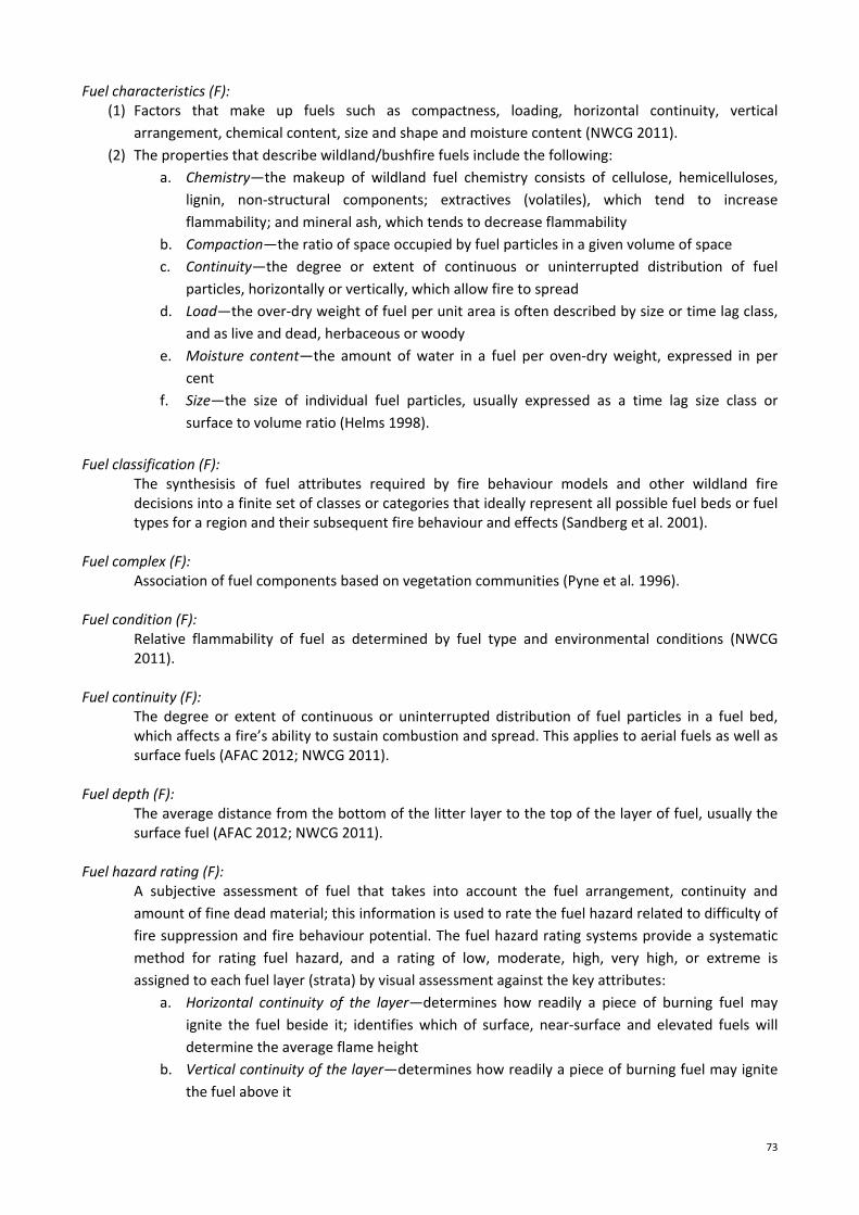
73
Fuel characteristics (F): (1) Factors that make up fuels such as compactness, loading, horizontal continuity, vertical
arrangement, chemical content, size and shape and moisture content (NWCG 2011).
(2) The properties that describe wildland/bushfire fuels include the following:
a. Chemistry—the makeup of wildland fuel chemistry consists of cellulose, hemicelluloses,
lignin, non‐structural components; extractives (volatiles), which tend to increase
flammability; and mineral ash, which tends to decrease flammability
b. Compaction—the ratio of space occupied by fuel particles in a given volume of space
c. Continuity—the degree or extent of continuous or uninterrupted distribution of fuel
particles, horizontally or vertically, which allow fire to spread
d. Load—the over‐dry weight of fuel per unit area is often described by size or time lag class,
and as live and dead, herbaceous or woody
e. Moisture content—the amount of water in a fuel per oven‐dry weight, expressed in per
cent
f. Size—the size of individual fuel particles, usually expressed as a time lag size class or
surface to volume ratio (Helms 1998).
Fuel classification (F):
The synthesisis of fuel attributes required by fire behaviour models and other wildland fire decisions into a finite set of classes or categories that ideally represent all possible fuel beds or fuel types for a region and their subsequent fire behaviour and effects (Sandberg et al. 2001).
Fuel complex (F):
Association of fuel components based on vegetation communities (Pyne et al. 1996).
Fuel condition (F): Relative flammability of fuel as determined by fuel type and environmental conditions (NWCG 2011).
Fuel continuity (F): The degree or extent of continuous or uninterrupted distribution of fuel particles in a fuel bed, which affects a fire’s ability to sustain combustion and spread. This applies to aerial fuels as well as surface fuels (AFAC 2012; NWCG 2011).
Fuel depth (F):
The average distance from the bottom of the litter layer to the top of the layer of fuel, usually the surface fuel (AFAC 2012; NWCG 2011).
Fuel hazard rating (F):
A subjective assessment of fuel that takes into account the fuel arrangement, continuity and
amount of fine dead material; this information is used to rate the fuel hazard related to difficulty of
fire suppression and fire behaviour potential. The fuel hazard rating systems provide a systematic
method for rating fuel hazard, and a rating of low, moderate, high, very high, or extreme is
assigned to each fuel layer (strata) by visual assessment against the key attributes:
a. Horizontal continuity of the layer—determines how readily a piece of burning fuel may
ignite the fuel beside it; identifies which of surface, near‐surface and elevated fuels will
determine the average flame height
b. Vertical continuity of the layer—determines how readily a piece of burning fuel may ignite
the fuel above it
74
c. Amount of dead material in the layer—determines how much dead material is present to
burn and help with igniting the live (green) fuels
d. Thickness of the fuel pieces—determines whether the fuel pieces will burn in the flaming
front of the fire
e. Total weight of the fine fuel—determines the weight of fire fuel contributing to the flaming
front of the fire (Hines et al. 2010).
Fuel hazard score (F):
A fuel hazard rating using a categorical score from 0 to 4 based on visual assessment of the percentage cover and fuel hazard for each fuel layer (strata) (See Figure A2). The fuel hazard score represents a subjective assessment of the flammability of each layer based on the type of bark, the density and morphological development of vegetation and accumulation of litter (Gould et al. 2007; 2011).
Fuel layer(s) (F): Visually obvious vertical fuel layers that can be associated with observed fire behaviour can be broadly identified by a change in bulk density (See Figure A2, example for eucalypt forest) (Gould et al. 2011).
Source: Gould et al. (2011)
Figure A2. Layers of fuel with the forest that can be identified visually. The grey scale on the side indicates the relative bulk density for each layer
Fuel load (F): (1) The oven dry weight of fuel per unit area. Commonly expressed as tonnes per hectare (t ha–1) (Also
known as fuel loading) (AFAC 2012).
(2) The amount of fuel present expressed quantitatively in terms of weight of fuel per unit area. This
may be available fuel (consumable fuel) or total fuels and is usually dry weight (NWCG 2011).
75
(3) The dry weight of combustible materials per unit area. Recommended SI units are kilograms per
square metre (kg m–2) or tonnes per hectare (t ha–1) (1.0 kg m–2 is equivalent to 10 t ha–1) (Merrill
and Alexander 1987):
10,000
11
1,000
Where: dryweight = dry weight of sample with container (g); container= weight of empty container (g), areaofquadrat= area from which fuel material was harvested or sampled (m2).
Fuel management (F): (1) Modification of fuel by prescribed burning or other means (AFAC 2012).
(2) The practice of controlling flammability and reducing resistance to control of wildland fuels through
mechanical, chemical, biological, or manual means, or by fire, in support of land management
objectives (NWCG 2011).
(3) The planned manipulation and/or reduction of living and dead forest fuel for forest management
and other land use objectives (e.g. hazard reduction, silvicultural purposes, wildlife habitat
improvement) by prescribed fire, mechanical, chemical, or biological means; and/or changing stand
structure and species composition (Merrill and Alexander 1987).
Fuel map (F):
A map showing areas of varying fuel quantities and types; usually indicating past fire history (AFAC 2012).
Fuel model (F):
Simulated fuel complex for which fuel descriptors required for the solution of a mathematical rate of spread model have been specified (AFAC 2012; NWCG 2011).
Fuel modification (F):
Manipulation or removal of fuels to reduce the likelihood of ignition and/or to lessen potential damage and resistance to control (e.g. lopping, chipping, crushing, piling and burning) (AFAC 2012; NWCG 2011).
Fuel moisture content (F):
The water content of a fuel expressed as a percentage of oven dry weight of the fuel particle (%OWD) (AFAC 2012):
%
100
Fuel moisture differential (F):
A term used to describe the situation where the difference in the moisture content between fuels on adjacent areas results in noticeably different fire behaviour on each area (AFAC 2005).
Fuel profile (F): The vertical cross section of a fuel bed down to mineral earth (AFAC 2012).
Fuel quantity (F):
SeeFuel load Fuel reduction (F):
Manipulation, including combustion, or removal of fuels to reduce the likelihood of ignition and/or to lessen potential damage and resistance to control (AFAC 2012; NWCG 2011).
76
Fuel reduction burning (F): The planned application of fire to reduce hazardous fuel quantities; undertaken in prescribed environment conditions with defined boundaries (AFAC 2012).
Fuel separation (F):
The action of separating fuel for the purpose of providing a mineral earth firebreak. Also means the actual gap between fuel layers or particles, e.g. gap between individual hummock grasses or gap between surface and canopy fuels (AFAC 2012).
Fuel size class (F):
A category used to describe the diameter of down woody fuels. Fuel within the same size class are assumed to have similar wetting and drying properties, and to preheat and ignite at similar rates during the combustions process (NWCG 2011).
Fuel treatment (F):
Manipulation or removal of fuels to reduce the likelihood of ignition and/or to lessen potential damage and resistance to control (e.g. lopping, chipping, crushing, piling, and burning (synonym—Fuel modification) (NWCG 2011).
Fuel type (F): (1) An identifiable association of fuel elements of distinctive species, form, size, arrangement, or other
characteristics that will cause predictable rate of spread of difficulty or control under specified
weather conditions (AFAC 2012; NWCG 2011).
(2) An identifiable association of fuel elements of distinctive species, form, size, arrangement and
continuity that will exhibit characteristic fire behaviour under defined burning conditions
(synonym—Fuel complex) (Merrill and Alexander 1987).
(3) An identifiable association of wildland/bushfire fuel elements of distinctive species, form, size,
arrangement, or other characteristics that will cause a predictable rate of spread or resistance to
control under specified weather conditions; kind of fuel include the following:
a. Activity fuels—the combustible material resulting from or altered by forestry
(management) practices such as timber harvesting or thinning, as opposed to naturally
created fuels
b. Aerial fuels— standing and supported live and dead combustible material not in direct
contact with the ground and consisting mainly of shrub and tree crowns, stems, foliage,
branches, and vines
c. Fine fuels—fast‐drying dead combustible material, generally characterised by a
comparatively high surface area‐to‐volume ratio and diameters of less than 6 mm, that is
consumed rapidly by fire when dry, e.g. grass, leaves, and needles, and time lag of one hour
or less
d. Ground fuels—combustible material below the surface fuel layer such as peat, duff, and
roots
e. Heavy fuels—combustible material or large diameter, usually > 70 mm that ignites and
burns more slowly the fire fuels (synonym—coarse fuel, coarse woody debris [CWD])
f. Ladder fuels—combustible material that provides vertical continuity between vegetation
strata and allows fire to climb into the crowns of trees or shrubs with relative easenote
ladder fuels help initiate and ensure the continuation of crown fire
g. Natural fuels—combustible material resulting from natural processes and not directly
generated or altered by land management practices
77
h. Surface fuels—the loose surface litter on the soil surface, e.g. fallen leaves or needles,
twigs, bark, cones, branches, grasses (Helms 1998).
Fuel weight (F):
See—Fuel load Fuelbreak (F):
(1) A natural or manmade change in fuel characteristics, affecting fire behaviour, so that fire burning
into them can be more readily controlled (AFAC 2012).
(2) An existing barrier or change in fuel type (to one that is less flammable than that surrounding it), or
a wide strip of land on which the native vegetation has been modified or cleared, that act as a
buffer to fire spread so that fires burning into then can be more readily controlled. Often selected
or constructed to protect a high value area from fires. In the event of fire, may serve as a control
line from which to carry out suppression operations (synonymFirebreak) (Merrill and Alexander
1987).
Fuelbreak system (G): A series of modified strips (or blocks grouped together) to form continuous strategically located fuel breaks around land units (AFAC 2012).
Grassfire (G):
(1) Any fire in which the predominant fuel is grass or grass‐like (AFAC 2012; Cheney and Sullivan 2008;
NWCG 2011).
Grassland (F):
Any land in which grasses dominate the vegetation (Cheney and Sullivan 2008). Grassland curing (G):
(1) The proportion of dead material in grassland, which usually increases over summer as tillers die
off and dry out, increasing the risk of grassland fire (AFAC 2012).
(2) The progressive senescence and drying out of a grass after flowering (annuals) or in response to
drought (perennials) (See—Curing) (Cheney and Sullivan 2008).
Ground fire (G):
Fire that consumes the organic material beneath the surface litter ground, such as a peat fire. (NWCG 2011)
Ground fuel (F): All combustible materials below the surface litter, including duff, roots, peat and sawdust dumps that normally support a glowing or smouldering combustion without flame (AFAC 2012; NWCG 2011).
Habitat (F):
The local environment of conditions in which an animal or plant lives (AFAC 2012). Hazard (F):
(1) A fuel complex defined by volume, type, condition, arrangement and location that determines
both the ease of ignition and of fire suppression difficulty (AFAC 2005).
(2) A source of potential harm or a situation with potential to cause loss (AFAC 2012).
(3) Any real or potential condition that can cause injury, illness or death of personnel, or damage to,
or loss of equipment or property (NWCG 2011).
78
Hazard fuel (F):
A fuel complex defined by kind, arrangement, volume, condition, and location that presents a threat of ignition and resistance to control (NWCG 2011).
Hazard reduction (F): See—Fuel management
Heat transfer (G):
The process by which heat is imparted from one body or object to another. In bush/forest fires, heat energy is transmitted from burning to unburnt fuels by:
Convection—transfer of heat by the movement of masses of hot air; the natural direction is upwards in the absence of any appreciable wind speed and/or slope Radiation—transfer of heat in straight lines from the warm surfaces to cooler surroundings Conduction—transfer of heat through solid matter (Merrill and Alexander 1987).
Heat yield (or Low heat or Combustion) (G):
The heat of combustion corrected for various heat losses arising from the presence of moisture in the fuel and incomplete combustion (Cheney and Sullivan 2008).
Heavy fuels (F):
Fuel of large diameter such as snags, logs, large limb wood, which ignite and are consumed more slowly than flash (fine) fuels. Also called Coarse fuels. (NWCG 2011)
Height (F): The vertical measurement of vegetation from the top of the crown to ground level. (NWCG 2011)
Herb (F): A plant that does not develop woody persistent tissue but is relatively soft or succulent and sprouts from the bases (perennials) or develops from seed (annuals) each year. Includes grasses, forbs, and ferns (NWCG 2011).
Humus (F): Layer of decomposed organic matter on the forest floor beneath the fermentation layer and directly above the soil. It is part of the duff, in which decomposition has rendered vegetation unrecognisable and mixing of soil and organic matter underway. See—Duff and Litter (AFAC 2012; NWCG 2011).
Hypothesis (S):
A proposition tentatively assumed in order to draw out its logical consequences and so test its validity after data are collected (Quinn and Keough 2002; USDI 2003).
Infrared (IR) imagery (G): A photograph‐like image created by optical‐electronic equipment using the infrared wavelength of the electromagnetic spectrum. In situations of fire, IR imagery is used to see through dense smoke, haze, and vegetation canopy to (a) detect the incidence of bushfires in remote terrain, especially following lightning storms, (b) map the perimeters, hot spots and spot fires of going fires and (c) detect residual heat sources during mop‐up; generally, the first two uses employ scanners in aircraft while the third uses hand‐held IR scanners on the ground or in slow‐flying helicopters (Helms 1998).
Integer (S): A number without a decimal; integer values can be less than, equal to or greater than zero (Helms 1998).
79
Intermediate tree and canopy layer (F):
Shorter trees with crowns either below or extending into lower part of the forest canopy. These may be immature individuals of overstorey species or species of intermediate stature that form a distinct layer beneath the co‐dominant of the overstorey species. Patches of regrowth trees in the open until they reach pole (co‐dominant) size. The intermediate tree layer can add a significant amount of bark fuel, and act as ladder fuel that can carries fires into the overstorey canopy (see Figure A2) (Gould et al. 2011).
Island (G):
An unburnt area within a fire perimeter (AFAC 2012). I Zone (G):
See—Urban–rural interface
Keetch‐Byram Drought Index (KBDI) (F): A numerical value reflecting the dryness of soils, deep forest litter, logs, and living vegetation; expressed as a scale from 0 to 200 (AFAC 2005; Keetch and Byram 1968).
Ladder fuels (F):
(1) Fuels that provide vertical continuity between strata. Fuel is able to carry surface fire into the
crowns of trees with relative ease (AFAC 2012, NWCG 2011).
(2) Fuels that provide vertical continuity between the surface fuels and crown fuels in forest stand,
contributing to the ease of torching and crowning (e.g. tall shrubs, small‐sized trees, bark flake, tree
lichen) (synonym—Bridge fuels) (Merrill and Alexander 1987).
Lag time (F):
The time delay in fuel moisture content responding to changing environmental conditions (for example, relative humidity). Technically, it is the time necessary for a fuel particle to lose approximately 63% of the difference between its initial moisture content and its equilibrium moisture content (AFAC 2012).
Land classification (F):
The process of generating and applying land strata that are sufficiently homogenous with respect to physical, vegetative and development attributes that the face validity of models and projections based on such strata is not threatened (Helms 1998).
Leaf area index (LAI) (F): The sum of all the upper or all‐sided leaf surface areas projected downward per unit area of ground beneath the canopy; the term has no units (Helms 1998).
Light fuel (F): (1) An assessment of fuel quantity indicating a low weight (AFAC 2012).
(2) Fast drying, generally with a comparatively high surface area‐to‐volume ratio, which are lass the
6 mm (1.4 in) in diameter and have a time lag of 1 hour or less. These fuels readily ignite and are
rapidly consumed by fire when dry (NWCG 2011).
Linear regression equation (S):
(1) Simple linear regression equation—a statistical model in which the expected value of response
variable is conditional on a single predictor variable and the model is linear in its parameters.
(2) Multiple linear regression equation—a statistical model in which the expected value of a response
variable is conditional on one or more response variables and the model is linear in its parameters.
80
(3) Nonlinear regression equation—a statistical model in which the expected value of a response
variable is conditional on one or more predictor variables and the model is nonlinear in its
parameters (Quinn and Keough 2002; Helms 1998).
Line‐intercept method (S):
The sampling of vegetation by recording the plants intercepted by a measured line set close to the
ground or by vertical projection from the line (Helms 1998).
Line transect (S):
(1) A sampling procedure employing lines of samples plots generally laid out at regular intervals along
a survey line (synonym—line‐plot survey) (Helms 1998).
(2) A sampling method consisting of horizontal, linear measurement of plant intercepts along the
course of a line. Transect data are typically used to measure foliar and basal cover. Also called line‐
intercept methods (USDI 2003).
Litter (F): (1) The top layer of the forest floor, composed of loose debris of dead sticks, branches, twigs and
recently fallen leaves and needles; its structure is little altered by decomposition (AFAC 2012;
Cheney and Sullivan 2008; NWCG 2011).
(2) Uppermost part of the forest floor consisting of freshly cast or slightly decomposed organic
materials (Merrill and Alexander 1987).
Litter bed fuel (f): Dead fine fuel, including surface fuel and fuel lower in the profile (AFAC 2012).
Litter fall (F):
The addition of litter that falls from vegetation to the forest floor (AFAC 2012). Live fuels (Living fuels) (F):
(1) Fuels made up of living vegetation. (AFAC 2012)
(2) Living plants, such as trees, grasses, and shrubs, in which the seasonal moisture content cycles
largely by internal physiological mechanisms, rather than external weather influences (NWCG
2011).
Live fuel moisture content (F):
Water content of a living fuel, expressed as a percentage of the oven‐dry weight of the fuel (USDI 2003).
Living shrub fuel (F): Living understorey fine fuels less than 2 metres above ground level (AFAC 2012).
Mean (S):
The average value of a series or set of observations obtained by dividing the algebraic sum of all observations in the set by the number of observations, often referred to as a measure of central location or central tendency (synonym—arithmetic mean) (Helms 1998).
∑
Where: = mean, = the observed value of the ith unit in the sample; =the number of units in the sample; ∑ describes the summation all of the ‐values in the sample (Quinn and Keough 2002).

81
Median (S):
The middle measurement in an ordered set of data; if the data contain an even number of items, then the median is the average of the two middle items (Helms 1998; Quinn and Keough 2002).
Medium fuels (F): Fuel too large to be ignited until after the leading edge of the fire front passes, but small enough to be completely consumed (synonym—Intermediate fuels). (See‐ Coarse fuels) (Merrill and Alexander 1987).
Methodology (S):
A set of standardised procedures and practices that have been peer‐reviewed and have received general acceptance by the profession (NWCG 2011).
Mineral soil (F): That portion of the soil stratum immediately below the litter and duff. Mineral soil contains very little combustible material except on highly productive sites where an upper soil horizon may be enriched with organic matter (NWCG 2011).
Mineral earth (G):
When used in the context of fire control, refers to a non‐flammable surface (either natural or prepared) that provides a break in understorey, litter and humus fuel and hence a barrier (of varied effectiveness depending, amongst other things, on its width and the intensity of the approaching fire) to fire travelling on or near the ground surface (AFAC 2012).
Mode (S):
The value occurring most frequently in a data set (Helms 1998; Quinn and Keough 2002).
Model (S): A simplified or generalised representation of reality, a description, analogy, picture or hypothesis to help visualise something that cannot be directly observed (NWCG 2011).
Model validation (S): The testing of a model by comparing model results with observation not used to develop the model (Helms 1998).
Moisture of extinction (F): The fuel moisture content, weighted over all the fuel classes, at which the fire will not spread. Also called extinction moisture content (EMC) (NWCG 2011).
Monitoring (S):
The collection of information over time, generally on a sample basis, by measuring change in an indicator or variable, to determine the effects of resource management treatment in the long term (Helms 1998).
Monte Carlo method (S):
(1) An analysis of data or simulation that relies on random sampling to generate values for probabilistic
components (Helms 1998).
(2) A technique in which a large quantity of randomly generated numbers are studied using a
probabilistic model to find an approximate solution to a numerical problem that would be difficult
to solve by other methods.

82
Mosaic (F): The intermingling of plant communities and their successional stages in such a manner as to give the impression of an interwoven design (NWCG 2011).
Multivariate analysis (S): The branch of statistics concerned with analysing multiple measurements that have been made on one or several variables (Helms 1998; Quinn and Keough 2002).
Native species (F): A species, which is a part of the original fauna or flora of the area in question (NWCG 2011).
Natural barrier (F): Any area where lack of flammable material obstructs the spread of vegetation fires (AFAC 2012, NWCG 2011).
Natural fire (G):
Any fire of natural origin (i.e. caused directly by lighting) (Merrill and Alexander 1987). Natural fuels (F):
Fuels resulting from natural processes and not directly generated or altered by land management practices (NWCG 2011).
Near‐surface fuel (F): (1) Live and dead fuel, including suspended leaves, bark, or twigs, effectively in touch with the ground
but not lying on it, with a mixture of vertical and horizontal orientation (AFAC 2012).
(2) Grasses, low shrubs, creepers, and collapsed understorey usually containing suspended leaf, twig,
and bark material from the overstorey vegetation. The height of this layer can vary from just
centimetres to over a metre above ground. Fuel layer components typically have a mixed
orientation ranging from horizontal to vertical and the layer is capable of suspending leaves, twigs
and bark above the ground (See Figure A2) (Gould et al. 2011).
Needle bed (F):
A fuel bed consisting mainly of pine needles (AFAC 2012). Normal distribution (S):
A commonly used probability distribution whose probability density function is symmetric and defined by two parameters, the mean and the variance (Helms 1998).
Null hypothesis (S): In a statistical test of significant the (usually equivalence) to a fixed value or to another parameter; in order to reject null hypothesis, a test statistic must indicate a sufficiently low probability (usually 0.05 or 0.01) of observing the sample data under the null hypothesis (Helms 1998).
One‐hour time lag fuels (1‐hr fuels) (F): Fuel consisting of dead herbaceous plant and round wood less than 6 mm (¼ inch ) in diameter. Also, includes the uppermost layer of needles or leaves on the forest floor (NWCG 2011).
One‐hour time lag fuel moisture (1‐hr FMC) (F): Moisture content of the one‐hour time lag fuels (NWCG 2011).

83
One‐hundred hour time lag fuels (100‐hr fuels) (F): Dead fuels consisting of round wood in size range of 25 to 70 mm (1 to 3 inches ) in diameter and very roughly the layer of litter extending from 2 mm to 100 mm (¾ to 4 inches) below the surface (NWCG 2011).
One‐hundred hour time lag fuel moisture (100‐hr FMC) (F): The moisture content of the 100‐hour fuels (NWCG 2011).
One‐thousand hour time lag fuel (1000‐hr fuels) (F): Dead fuels consisting of round wood greater than 70 mm (3 inches) in diameter and the layer of the forest floor more than 100 mm (4 inches ) below the surface (NWCG 2011).
One‐thousand hour time lag fuel moisture (1000‐hr FMC) (F): The fuel moisture content of the 1000‐hr fuels (NWCG 2011).
Organic matter (F):
The fraction of the soil that includes plant and animal residues at various stages of decomposition, cells and tissues of soil organism, and substances synthesised by the soil population (NWCG 2011).
Organic soil (F): Any soil or soil horizon containing at least 30% organic matter (e.g. peat) (NWCG 2011).
Overstorey tree and canopy layer (F): (1) Dominant and co‐dominant trees forming the uppermost canopy layer of the forest or woodlands.
The flammability of this layer depends primarily on the bark characteristics of the overstorey tree
species, and the height and density of the forest. The bark type of different species can have a large
impact on the rate of surface fuel accretion, transfer of surface fire into the canopy and the
generation of firebrands (see Figure A2) (Gould et al. 2011).
(2) That portion of the tree, in a forest of more than one storey, forming the upper or uppermost
canopy layer (Helms 1998).
Pace (S):
A unit of linear measure equal to the length of a given person’s stride. The pace is measured from the heel of one foot to the heel of the same foot in the next stride (USDI 2003).
Particle size (F): The size of a piece of fuel, often expressed in terms of size classes (NWCG 2011).
Peat (F): An amorphous organic material formed by anaerobic decomposition, which usually means that the area is seasonally or permanently inundated with water. Peat fires burn by smouldering combustion and generate very high amounts of energy per unit area (AFAC 2012).
Plot (S):
The experimental unit to which a treatment may be randomly assigned (Helms 1998).
Precision (S): (1) The closeness (to each other) of repeated measurements of the same quantity.
(2) The exactness of measurement; e.g. the measurement of 123.45 is more precise than the
measurement of 123.5.
(3) The statistical representation for the standard deviation of a number of measurements (Helms
1998).

84
(4) A measure of how close an estimator is expected to be to the true value of a parameter; standard
error is also called the ‘precision of the mean’ (USDI 2003).
Prescribed burning (G):
(1) The controlled application of fire under specified environmental conditions to a predetermined
area and for the time, intensity, and rate of spread required to attain planned resource
management objectives (AFAC 2012; NWCG 2011).
(2) The knowledgeable application of fire to a specific land area to accomplish predetermined forest
management or other land use objective (synonym—Fire use) (Merrill and Alexander 1987).
Prescribed fire (G):
(1) Any fire ignited by management action to meet a specific objective. A written approved burn plan
must exist, and approving agency requirements (where applicable) must be met, prior to ignition
(AFAC 2012; NWCG 2011).
(2) Any fire deliberately used for prescribed burning; usually set by qualified fire management
personnel according to a predetermined burning prescription. Notein some cases a wildfire that
may produce beneficial results in terms of the attainment of forest management or other land use
objective may be allowed to burn under certain burning conditions according to a predefined
burning prescription, with limited or no suppression action, and as such may be considered a form
of prescribed fire (Merrill and Alexander 1987).
Prescribed fire burn plan (G):
A plan required for each fire application deliberately lit as part of a fire management strategy. Plans are documents prepared by qualified personnel, approved by the agency administrator, and include criteria for the conditions under which the fire will be conducted (a prescription). Plan content varies among the agencies (NWCG 2011).
Prescription (G): Measurable criteria that define conditions under which a prescribed fire may be ignited, guide selection of appropriate management responses, and indicated other required actions (NWCG 2011).
Probability (S): (1) A number representing the chance that a given event will occur. The range is from 0% from an
impossible event to 100% for an inevitable event (also considered in terms of 0 to 1) (NWCG 2011).
(2) The relative frequency of a specific event, expressed as a proportion of per cent of the total
number of events (Helms 1998).
Profile litter moisture content (F):
The moisture content, expressed as a percentage of oven‐dry weight, of the entire leaf litter bed above the mineral soil surface (AFAC 2012).
Quadrat (S)
A small, clearly demarcated sample area of any shape but known size, on which observation or samples are made (Helms 1998).
Qualitative variable (S): A variable for which an attribute or classification is assigned, e.g. height class, age class, fuel hazard rating (USDI 2003).

85
Quantitative variable (S): A variable for which a numeric value representing an amount is measured, e.g. cover, density, fuel hazard score (USDI 2003).
Radiant heat flux (G): The amount of heat flowing through a given area in a given time, usually expressed as calories/square centimetre/second) (NWCG 2011).
Radiation (G): (1) Propagation of energy in free space by virtue of joint undulating variation in the electric or
magnetic fields in space (i.e. by electromagnetic waves).
(2) The transfer of heat in straight lines through a gas or vacuum other than by heating of the
intervening space (NWCG 2011).
Random sample (S):
A technique involving the selection of a group of plots (a sample) for study from a larger group (a population). Sampled individuals are chosen entirely by chance; each member of the population has a known, but possibly non‐equal chance of being included in the sample. Thus, use of random sampling generates credible results with introducing significant bias (Quinn and Keough 2002; USDI 2003).
Rate of area growth (G): The speed at which a fire increases its size, expressed in terms of area per unit of time. Recommended SI units are hectares per hour (ha h–1) (Merrill and Alexander 1987).
Rate of perimeter growth (G):
The speed at which a fire increases its perimeter, expressed in terms of distance per unit of time. Recommended SI units are metres per minute (m min–1) and kilometres per hour (km h–1) (synonym—Rate of perimeter increase (Merrill and Alexander 1987).
Rate of spread (ROS) (G):
(1) The relative activity of a fire extending its horizontal dimensions. It is expressed as rate of increase
of the total perimeter of the fire, as rate of forward spread of the fire front, or as a rate of increase
in area, depending on the intended use of the information. Usually it is expressed in metres or
hectares per hour for a specific period in the fire’s history (NWCG, 2011).
(2) The relative activity of a fire extending its horizontal dimension. Expression either as increase of the
fire perimeter (expressed as: m min–1, m hr–1, km hr–1), as rate of increase in area (m2 min–1, m2 hr–1,
ha hr–1) or as a rate of advance of its headrate of forward spread, (expressed as: m min–1, m hr–1,
km h–1), depending on the intended use of the information (Cheney and Sullivan 2008).
(3) The speed at which a fire extends its horizontal dimensions, expressed in terms of distance per unit
of time. Generally thought of in terms of a fire’s forward movement or head fire rate of spread, but
also applicable to backfire and flank fire ROS. Recommended SI units are metres per minute
(m min–1) and kilometres per hour (km h–1) (1.0 m min–1 is equivalent to 0.06 m hr–1) (Merrill and
Alexander 1987).
Rate of spread meter (G):
A device that computes the probable rate of spread of a fire for different combinations of fuel moisture, wind speed, and other selected factors (NWCG 2011).
86
Reaction intensity (G): The rate of heat release, per unit of the flaming fire from, expressed as heat energy/area/time, i.e. Kcal/square meter/second (NWCG 2011)
Regeneration burn (G): A burn lit under prescribed conditions for the purpose of achieving regeneration of a particular vegetation (AFAC 2012).
Regression (S):
A statistical measure of the amount of change in a dependent variable and one or more independent variables; generally expressed as a regression equation (Quinn and Keough 2002; Helms 1998).
Regression coefficient (S): The multiplier of an independent variable in a regression equation (Helms 1998; Quinn and Keough 2002).
Representativeness (S): The ability of a given sample to represent the total population from which it was taken (USDI 2003).
Residence time (G): (1) The time required for the flaming zone of a fire to pass a stationary point; the width of the flaming
zone divided by the rate of spread of the fire (AFAC 2012).
(2) The time, in seconds, required for the flaming front of a fire to pass stationary point at the surface
of the fuel. The total length of time that the flaming front of the fire occupies one point (NWCG
2011).
(3) The length of time required for the flaming zone or fire front of a spreading fire to pass a given
point, most commonly expressed in minutes (min) and/or seconds (s). Numerically, it is equal to
the flame depth divided by the rate of spread (Merrill and Alexander 1987).
Resistance to control (G):
(1) The relative difficulty of constructing and holding a control line as affected by resistance to line
construction and by fire behaviour. Also called difficulty of control (NWCG 2011).
(2) The relative ease of establishing and holding a fireguard and/or securing a control line as
determined by the difficulty of control and resistance to fireguard construction (Merrill and
Alexander 1987).
Risk (G):
(1) The exposure to the possibility of such things as economic or financial loss or gain, physical
damage, injury or delay, as a consequence of pursuing a particular course of action. The concept of
risk has two elements, i.e. the likelihood of something happening and the consequences if it
happens (AFAC 2012).
(2) The ISO 31000 (2009)/ISO Guide 73:2002 definition of risk is the ‘effect of uncertainty on
objectives’.
Risk analysis (G):
A systematic use of available information to determine how often specific events may occur and the magnitude of their likely consequences (AFAC 2012).
87
Root mean square error (RMSE) (S): The square root of the average of the squared differences of the value from their means (Helms 1998).
Rural (G):
Any area wherein residences and other development are scattered and intermingled with forest, range or farmland and native vegetation or cultivated crops (AFAC 2012; NWCG 2011).
Sample (S):
(1) Part of a population; that portion of the population that is measured (NWCG 2011).
(2) A part of a population consisting of one or more sampling units and examined as representative of
the whole.
(3) To select and measure or record a sample of the population (Helms 1998).
Sample mean (S):
The arithmetic mean of a random variable in a sample, calculated by dividing the sum of observations by their number (Helms 1998; Quinn and Keough 2002).
Sample plot (S):
An area of a stand, forest or plant community chosen as representative of a much greater area (Helms 1998).
Sample size (S): The number of items or observations in a sample, usually denoted by lower case letter n (NWCG 2011).
Sample, stratified (S):
A sample taken by selecting sample units from each of several strata (Helms 1998).
Sample, systematic (S): A sample consisting of units selected according to a geometric or other non‐random procedure (Helms 1998).
Sampling error (S): The difference between a population value and a sample estimate that is attributable to the sample, as distinct from errors due to bias in estimation or errors in observation. Sampling errors is measured as the standard error of the sample’s estimates (Helms 1998).
Savanna (F): Lowland, tropical or subtropical grassland, generally with a scattering of trees or shrubs (Helms 1998).
Savanna woodland (F): A more or less open tropical or subtropical woodland having an undergrowth mainly of grasses, being of moderate height (Helms 1998).
Scorch height (G): (1) The height above ground level up to which foliage has been browned by a fire.
(2) A measurement for determining the acceptable height of flame during prescribed burning (AFAC
2012).
(3) Average heights of foliage browning or bole blacking caused by a fire (NWCG 2011).

88
Scrub (F): (1) Refers to vegetation such as heath, wiregrass and shrubs, which grows either as an understorey or
by itself in absence of a tree canopy (AFAC 2012).
(2) A collective term that refers to stands of vegetation dominated by shrubby woody plants or low‐
growing trees (Cheney and Sullivan 2008).
(3) A formation that is dominated by shrubs, usually multi‐stemmed, with foliage project cover of
70‐100% for close scrub, and 30‐70 % for open scrub; 10‐30% foliage projected cover; with a height
2–8 metres (tall shrubland) or for low shrubland, a height up to 2 metres tall (Specht and Specht
1999).
Scrub fire (F):
Fires burning in scrub (AFAC 2012).
Shrub (F) (1) A woody perennial plant differing from a perennial herb by its persistent and woody stem, and
from a tree by its low stature and habit of branching from the base (NWCG 2011).
Slash (F):
(1) Accumulated fuel resulting from such natural events as wind, fire, snow breakage, or from such
human activities as logging, cutting or road construction (AFAC 2012).
(2) Debris resulting from such natural events as wind, fire, or snow breakage, or such human activities
as road construction, logging, pruning, thinning or brush clearing. Includes logs, chunks for bark,
branches, stumps and broken understory trees or brush (NWCG 2011).
(3) Unusual concentration of fuel resulting from such natural events as wind or snow breakage of
trees.
(4) Fuels resulting from human activities such as logging, thinning or road construction (Cheney and
Sullivan 2008).
(5) Debris left as a result of forest and other vegetation being altered by forestry practices and other
land use activities (e.g. timber harvesting, thinning and pruning, road construction, land clearing).
Includes material such as logs, splinters, or chops, tree branches and tops, uprooted stumps and
broken or uprooted trees and shrubs (Merrill and Alexander 1987).
Slash burn (G):
A prescribed burn conducted to consume slash for fire hazard reduction or silvicultural purposes. Snag (F):
A standing dead tree or part of a dead tree from which at leaves and smaller branches have fallen (NWCG 2011).
Softwood (F): A conventional term used to describe a tree, and the timber of trees, belonging to the group of plants with cones, such as pine or cypress (AFAC 2012).
Soil dryness index (SDI) (F): A measure of the soil profile dryness (AFAC 2005; Mount 1972).
Spatial data (S):
Information about the location and shape of, geographic features, and relationships among them, usually stored as coordinates and topology (Helms 1998).

89
Specific heat (G):
The heat required to raise a unit mass of a substance in one degrees Kelvin. It is the heat capacity of a system per unit mass; i.e. the ratio of the heat absorbed (or released) to the corresponding temperature rise (or fall) (NWCG 2011).
Spot fire (G): (1) Isolated fire started ahead of the main fire by sparks, embers or other ignited material, sometimes
to a distance of several kilometres.
(2) A very small fire that requires little time or effort to extinguish (AFAC 2012).
(3) Fire ignited outside the perimeter of the main fire by a firebrand (NWCG 2011).
(4) A fire ignited by firebrands that are carried outside the main fire perimeter by air currents, gravity,
and/or fire whirls (Merrill and Alexander 1987).
Spot ignition (G):
An ignition pattern using a series of spaced points of ignition (AFAC 2012). Spotting (G):
Behaviour of a fire producing sparks or embers that are carried by the wind and start a new fire beyond the zone of direct ignition by the main fire (AFAC 2012; NWCG 2011).
Standard deviation (S):
A measure of the dispersion about the mean of a population or sample, i.e. the positive square root of the variance and represented as s (Helms 1998).
∑ 1
Where: = standard deviation, = number of observations within the sample, = the ith sample observation, = sample mean (Quinn and Keough 2002).
Standard error (S): The standard deviation of the values of a given function of the data (parameter), overall possible samples of the same size, represented by se (USDI, 2003).
√
where: = standard error, = standard deviation, = number of plots or samples (Quinn and Keough 2002).
Stand density (F): (1) A quantitative measure of stocking expressed either absolutely in terms of number of trees, basal
area, or volume per unit area or relative to some standard condition.
(2) A measure of the degree of crowning of trees within stocked areas commonly expressed by various
growing space ratios (Helms 1998).
Stand replacing fire (G):
Fire that kills all or most of the living overstorey trees in a forest and initiates forest succession or regrowth. Also explicitly describes the nature of fire in grasslands and some shrublands (NWCG 2011).
90
Stratified random sample (S): A sample drawn from a stratified population consisting of a random sample from each stratum and permitting the sampling to vary by stratum to (a) improve efficiency of sampling, (b) obtain separate estimates for strata, or (c) improve the precision of the population (Helms 1998; Quinn and Keough 2002).
Stratum (strata) (F): (1) A distinct layer of vegetation with a plant community.
(2) A subdivision of a population, used in stratified sampling (Helms 1998).
Structure (G):
A constructed object, usually a freestanding building above ground (AFAC 2012; NWCG 2011). Succession (F):
The process of vegetation development whereby an area becomes successively occupied by different plant communities of higher ecological order (NWCG 2011).
Surface area–to‐volume ratio (F):
The ratio between the surface area of an object, such as a fuel particle, to its volume. The smaller the particle, the more quickly it becomes wet, dries out, or can become heated to combustion temperature during a fire (NWCG 2011).
Surface fire (G): Fire that burns loose debris on the surface, which includes dead branches, leaves and low
vegetation (AFAC 2012; NWCG 2011).
Surface fuel (layer) (F):
(1) Leaves, twigs and bark of overstorey and understorey plants. Fuel components are generally
horizontally layered. This layer usually makes up the bulk of the fuel consumed and provides most
of the energy released by a fire. Surface fuel burns by both flaming and smouldering combustion,
and determines the flame depth of a surface fuel (see Figure A2) (Gould et al. 2011).
(2) Litter fuels made up of leaves, twigs, bark and other fine fuel lying on the ground, predominately
horizontal in orientation (AFAC 2012).
(3) Fuels lying on or near the surface of the ground consisting of leaf and needle litter, dead branch
material, downed logs, bark, tree cones and low‐stature living plants (NWCG 2011).
(4) All combustible materials lying above the duff layer between the ground and ladder fuels that are
responsible for propagating surface fires (e.g. litter, herbaceous vegetation, low and medium
shrubs, tree seedling, stumps, downed‐dead round material) (Merrill and Alexander 1987).
Surface moisture content (F):
The moisture content expressed as a percentage of oven dry weight of the top 5–10 mm of leaf litter (AFAC 2012).
Test of significance (S):
A computation of the probability that an observed effect or difference may have arisen purely as a result of chance or as a result of experimental errors; if this probability is less than an agreed small value (termed the level of significance and often accepted as 1:20), the effect or difference is said to be significant, leading to a decision to accept or reject the statistical hypothesis under consideration; a non significant result does not, however, constitute a proof that the result is due to chance only (Helms 1998; Quinn and Keough 2002).
91
Ten‐hour time lag fuels (10‐hr fuels) (F): Dead fuels consisting of round wood 6 to 25 mm (¼ to 1‐in) in diameter and, very roughly, the layer of litter extending from immediately below the surface to 2 mm (¾‐in) below surface. (NWCG 2011)
Ten‐hour time fuel moisture (10‐hr FMC) (F):
The fuel moisture content of the 10‐hr time lag fuels (NWCG 2011).
Thermal imagery (S): The display or printout of an infrared scanner operating over a fire. Also called infrared imagery (NWCG 2011).
Timelag (F):
Time needed under specified conditions for a fuel particle to lose about 63 per cent of the difference between its initial moisture content and its equilibrium moisture content. If conditions remain unchanged, a fuel will reach 95 per cent of its equilibrium moisture after four timelag periods (NWCG 2011).
Total fuel (F): (1) All plant material both living and dead that can burn in a worst‐case situation (NWCG 2011).
(2) The quantity of fuel, which would burn under the driest conditions with the highest‐intensity fire.
The virtue of introducing the concept of total fuel is that it set a maximum value for the available
fuel. Total fuel is measured in the same units as available fuel (Byram 1959).
Total fine fuel (F):
The total fuel quantity of fine fuels (<6mm) in the surface, near‐surface and elevated fuel layers (Gould et al. 2011).
Total fuel energy (F):
Bears the same relationship to the available fuel energy as does total fuel to available fuel (Byram 1959).
Transect (S): A narrow sample strip or a measured line laid out through vegetation specifically chosen for sampling (Helms 1998).
Underburn (G): A fire that consumes surface fuels but not overstorey canopy (NWCG 2011).
Understorey (F): All forest vegetation growing under an overstorey (Helms 1998).
Urban (G): Area in which residence and other human development form an essentially contiguous covering of the landscape, includes most area within cities and towns, subdivisions, commercial and industrial parks, and similar development whether inside city limits or not (AFAC 2012).
Urban–rural interface (URI) (F):
The line, area, or zone where structures and other human development adjoin or overlap with
underdeveloped bushland (synonymWildland–urban interface, WUI) (AFAC 2012). Values at risk (G):
(1) Natural resources or improvements that may be jeopardised if a fire occurs (AFAC 2012).
92
(2) Include property, structure, physical improvements, natural and culture resources, community
infrastructure, and economic, environmental and social values. Also known as values to be
protected (NWCG 2011).
(3) The specific or collective set of natural resource and man‐made improvement/developments that
have measurable or intrinsic worth and that could or may be destroyed or otherwise altered by
fires in any given area (Merrill and Alexander 1987).
Variable (S):
(1) Any changing characteristics, in statistics; measurable characteristics of an experimental unit
(NWCG 2011).
(2) Any quantity that varies.
(3) A quantity that may take any one of a specific set of values (Helms 1998).
Variance (S):
A statistical measure of the variation of a characteristic from the population mean; the expected value of the squared difference between a statistic and the expected value of that statistic (Helms 1998; Quinn and Keough 2002).
Vigour (F): A subjective assessment of the health of individual plants in similar and growing conditions; or a more specific measure based upon a specific facet of growth, such as seed stalk, or tiller production per plant or per unit area (NWCG 2011).
Visual estimation (S): A method of quantifying a variable; species cover is visually estimated either in the entire study area, or within sample plots, such as in quadrates (USDI 2003).
Volatiles (F): Readily vaporised organic materials which, when mixed with oxygen, are easily ignited (NWCG 2011).
Weighted mean (S): A type of average that takes into account the differing weights of the observations; the summed product of the values times their weights divided by the sum of the weights (Helms 1998).
Wildfire (G): An unplanned, unwanted wildland fire including unauthorised human‐caused fires, escaped wildland fire use events, escaped prescribe fire project and all other wildland fire where the objective is to put the fire out (NWCG 2011).
Wildland (G): (1) An unplanned vegetation fire. A generic term, which includes grass fires, forest fires and scrub fire
both with and without a suppression objective (SeeBushfires) (AFAC 2012).
(2) An area in which development is essentially non‐existent, except for road, railroads, powerlines,
and similar transport facilities. Structures, if any, are widely scattered (NWCG 2011).
Wildland fire (G):
Any non‐structured fire that occurs in the wildland. Three distinct types of wildland fire have been defined and include wildfire, wildland fire use, and prescribed fire (NWCG 2011).

93
Wilderness area (G): Places where wilderness quality defined using thresholds of remoteness, naturalness and total area is recognised and valued by society (AFAC 2012).
Wildland–urban interface (WUI) (F):
SeeUrban–rural interface Windfall (F):
A tree or trees that have been uprooted or broken off by wind, or an area of previously standing
timber that has be blown over by strong winds or storms (synonymBlowdown) (Merrill and Alexander 1987).
Wind throw (F):
An area of previously standing timber, which has been blown over by strong winds or storms (AFAC 2012).
Windrow (F):
A long line of piles or debris resulting from forest or scrub clearing (AFAC 2012). Windrow burning (G):
(1) The burning of windrows (AFAC 2012).
(2) Burning slash that has been piled into long continuous rows. Also includes wildfire in vegetation
planted to protect improvements or agriculture (NWCG 2011).
Woodland (F):
(1) A subset of forest plant communities, within which the trees form only an open canopy
(Between 20% and 50% crown cover), the intervening area being occupied by lower vegetation,
usually grass or scrub (AFAC 2012).
(2) An area with trees (>5 m) with a projected foliage cover of 30% or less (10–30% = woodland, < 10% open woodland), 5–10 m = low woodland, > 30 m = tall woodland (Specht and Specht 1999).
94
References Australasian Fire and Emergency Services Authorities Council (AFAC) 2005, Conduct prescribed burning:
learner resource, PUAFIRE407B, AFAC, East Melbourne. Australasian Fire and Emergency Services Authorities Council (AFAC) 2012, Bushfire glossary, AFAC, East
Melbourne, viewed 12 January 2012, http://knowledgeweb.afac.com.au/data/documents/AFAC_Bushfire_Glossary_ Indexed_2012.pdf>.
Andrews, PL & Queen, LP, 2001, ‘Fire modelling and information system technology’, International Journal
of Wildland Fire, vol. 10, pp. 343–353.
Bureau of Meteorology (BoM 2012), Glossary, viewed June 2012, <http://www.bom.gov.au/lam/glossary>. Burgan, R, Klaver, R & Klaver, J 1998, ‘Fuel model and fire potential from satellite and surface observations’,
International Journal of Wildland Fire, vol. 8, pp. 159–170. Byram, GM 1959, ‘Combustion of forest fuels’, in KP Davis (ed.), ‘Forest fire control and use’, McGraw‐Hill
Book Company Inc., New York, pp. 61–89.
Cheney, P & Sullivan, A 2008, Grassfiresfuel weather and fire behaviour, 2nd edn, CSIRO Publishing, Collingwood, Victoria.
Cochran, WG 1977, Sample techniques, 3rd edn, Wiley, New York.
Gould, JS, McCaw, WL, Cheney, NP, Ellis, PE & Matthews, S 2007b, Field guidefuel assessment and fire behaviour prediction in dry eucalypt forest, Ensis‐CSIRO, Canberra, & Department of Environment and Conservation, Perth.
Gould, JS, McCaw, WL & Cheney, NP 2011, ‘Quantifying fine fuel dynamics and structure in dry eucalypt
forest (Eucalyptus marginata) in Western Australia for fire management’, Forest Ecology and Management, vol. 262, pp. 531–546.
Helms, JA (ed.) 1998, The dictionary of forestry, Society of American Foresters, Bethesda, Maryland. Hines, F, Tolhurst, KG, Wilson, AAG & McCarthy, GJ 2010, Overall fuel hazard assessment guide, 4th edn,
Department of Sustainability and Environment, Melbourne.
Husch, B, Miller, CI & Beers, TW 1972, Forest mensuration, 2nd edn, The Ronal Press Company, New York.
Keetch, JJ, Byram, GM 1968. A drought index for forest fire control, Research Paper SE‐38, USDA Forest
Service, Ashville, North Carolina. Mandallaz, D 2008, Sampling techniques for forest inventories, Chapman & Hall/CRC, New York.
Merrill, DF & Alexander, ME 1987, Glossary of forest fire management terms, 4th edn, NRCC no. 26515, Canadian Committee on Forest Fire Management, National Research Council of Canada, Ottawa.

95
Mount, AB 1972, The derivation and testing of a soil dryness index using run‐off data, Bulletin no. 4, Tasmania Forest Commission, Hobart.
NWCG 2011, Glossary of wildland fire terminology, PMS 205, National Wildfire Coordinating Group, Boise,
Idaho <http://www.nwcg.gov/pms/pubs/glossary/index.htm>. Quinn, GP & Keough, MJ 2002, Experimental design and data analysis for biologists, Cambridge University
Press, Cambridge, United Kingdom.
Pyne, SJ, Andrews, PL & Laven, RD 1996, Introduction to wild fire, 2nd edn, John Wiley & Sons Inc. New York.
Sandberg, DV, Ottmar, RD & Cushon, GH 2001, ‘Characterizing fuels in the 21st century’, International
Journal of Wildland Fire, vol. 10, pp. 381–387.
Specht, RL & Specht, A 1999, Australian plant communities: dynamics of structure, growth, and biodiversity,
Oxford University Press. United States Department of Interior (USDI) 2003, Fire monitoring handbook, USDI National Park Service,
Fire Management Program, National Interagency Fire Centre, Boise, Idaho.
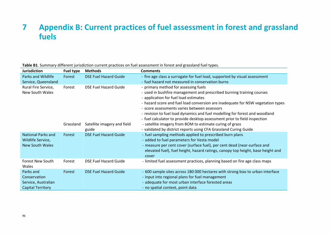
96
7 Appendix B: Current practices of fuel assessment in forest and grassland fuels
Table B1. Summary different jurisdiction current practices on fuel assessment in forest and grassland fuel types.
Jurisdiction Fuel type Methods Comments
Parks and Wildlife Service, Queensland
Forest DSE Fuel Hazard Guide ‐ fire age class a surrogate for fuel load, supported by visual assessment ‐ fuel hazard not measured in conservation burns
Rural Fire Service, New South Wales
Forest Grassland
DSE Fuel Hazard Guide Satellite imagery and field guide
‐ primary method for assessing fuels ‐ used in bushfire management and prescribed burning training courses ‐ application for fuel load estimates ‐ hazard score and fuel load conversion are inadequate for NSW vegetation types ‐ score assessments varies between assessors ‐ revision to fuel load dynamics and fuel modelling for forest and woodland ‐ fuel calculator to provide desktop assessment prior to field inspection ‐ satellite imagery from BOM to estimate curing of grass ‐ validated by district reports using CFA Grassland Curing Guide
National Parks and Wildlife Service, New South Wales
Forest DSE Fuel Hazard Guide ‐ fuel sampling methods applied to prescribed burn plans ‐ added to fuel parameters for Vesta model ‐ measure per cent cover (surface fuel), per cent dead (near‐surface and elevated fuel), fuel height, hazard ratings, canopy top height, base height and cover
Forest New South Wales
Forest DSE Fuel Hazard Guide ‐ limited fuel assessment practices, planning based on fire age class maps
Parks and Conservation Service, Australian Capital Territory
Forest DSE Fuel Hazard Guide ‐ 600 sample sites across 180 000 hectares with strong bias to urban interface ‐ input into regional plans for fuel management ‐ adequate for most urban interface forested areas ‐ no spatial context, point data
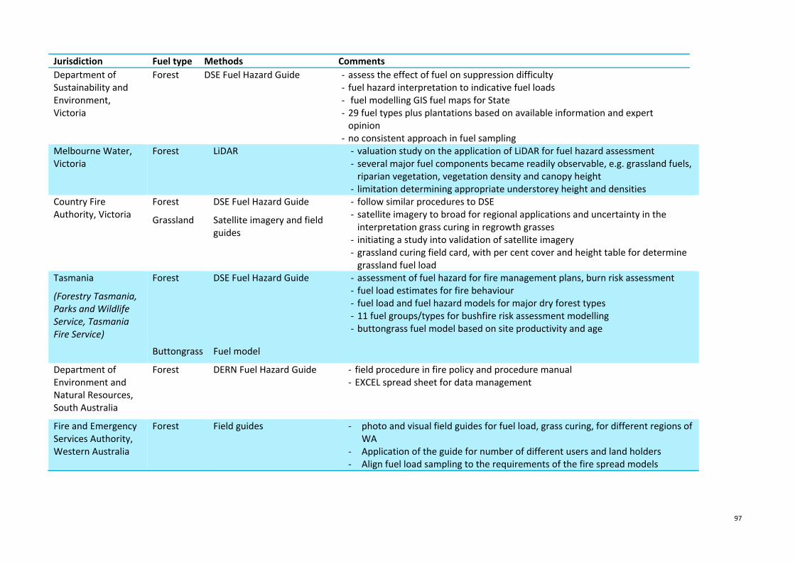
97
Jurisdiction Fuel type Methods Comments
Department of Sustainability and Environment, Victoria
Forest DSE Fuel Hazard Guide ‐ assess the effect of fuel on suppression difficulty ‐ fuel hazard interpretation to indicative fuel loads ‐ fuel modelling GIS fuel maps for State ‐ 29 fuel types plus plantations based on available information and expert opinion
‐ no consistent approach in fuel sampling Melbourne Water, Victoria
Forest LiDAR ‐ valuation study on the application of LiDAR for fuel hazard assessment ‐ several major fuel components became readily observable, e.g. grassland fuels, riparian vegetation, vegetation density and canopy height
‐ limitation determining appropriate understorey height and densities Country Fire Authority, Victoria
Forest
Grassland
DSE Fuel Hazard Guide
Satellite imagery and field guides
‐ follow similar procedures to DSE ‐ satellite imagery to broad for regional applications and uncertainty in the interpretation grass curing in regrowth grasses
‐ initiating a study into validation of satellite imagery ‐ grassland curing field card, with per cent cover and height table for determine grassland fuel load
Tasmania
(Forestry Tasmania, Parks and Wildlife Service, Tasmania Fire Service)
Forest
Buttongrass
DSE Fuel Hazard Guide
Fuel model
‐ assessment of fuel hazard for fire management plans, burn risk assessment ‐ fuel load estimates for fire behaviour ‐ fuel load and fuel hazard models for major dry forest types ‐ 11 fuel groups/types for bushfire risk assessment modelling ‐ buttongrass fuel model based on site productivity and age
Department of Environment and Natural Resources, South Australia
Forest DERN Fuel Hazard Guide ‐ field procedure in fire policy and procedure manual ‐ EXCEL spread sheet for data management
Fire and Emergency Services Authority, Western Australia
Forest Field guides ‐ photo and visual field guides for fuel load, grass curing, for different regions of WA
‐ Application of the guide for number of different users and land holders ‐ Align fuel load sampling to the requirements of the fire spread models

98
Jurisdiction Fuel type Methods Comments
Department of Environment and Conservation, Western Australia
Forest, Mallee heath, grasslands
Field guides and field surveys ‐ Vesta fuel hazard guide and fuel age maps (Vesta fire spread model) ‐ fuel load for Forest Fire Behaviour Tables, WA ‐ different procedures depending on fuel type (forest, mallee heath, hummock
grassland, grasslands) ‐ line transect, destructive fuel sampling ‐ 19 major fuel types
Bushfire Council, Northern Territory
Grassland North Australian Grassland Fuel Guide
‐ photo guide on curing and fuel load ‐ fuel sampling to estimate fuel load (woody fuels, leaf litter, grass, shrubs)


100
CONTACT US
t 1300 363 400 +61 3 9545 2176 e [email protected] w www.csiro.au
YOUR CSIRO
Australia is founding its future on science and innovation. Its national science agency, CSIRO, is a powerhouse of ideas, technologies and skills for building prosperity, growth, health and sustainability. It serves governments, industries, business and communities across the nation.
FOR FURTHER INFORMATION
Ecosystem Sciences/Bushfire Dynamic and Application Group Jim Gould t +61 2 6246 4220 e [email protected] Ecosystem Science/Bushfire Dynamics and Application Group Miguel Cruz t +61 2 6246 4219 e [email protected]