audit of douglas county assessor fy 2007/2008 #05 douglas county

SIAM J. NUMER. ANAL. c© 2005 Society for Industrial and Applied MathematicsVol. 43, No. 2, pp. 623–644

SPECTRAL APPROXIMATION OF THE HELMHOLTZ EQUATIONWITH HIGH WAVE NUMBERS∗

JIE SHEN† AND LI-LIAN WANG†

Abstract. A complete error analysis is performed for the spectral-Galerkin approximation ofa model Helmholtz equation with high wave numbers. The analysis presented in this paper doesnot rely on the explicit knowledge of continuous/discrete Green’s functions and does not requireany mesh condition to be satisfied. Furthermore, new error estimates are also established for multi-dimensional radial and spherical symmetric domains. Illustrative numerical results in agreementwith the theoretical analysis are presented.

Key words. Helmholtz equation, high wave numbers, spectral-Galerkin approximation, erroranalysis

AMS subject classifications. 65N35, 65N22, 35J05, 65F05

DOI. 10.1137/040607332

1. Introduction. Time harmonic wave propagations appear in many applica-tions, e.g., wave scattering and transmission, noise reduction, fluid-solid interaction,and sea and earthquake wave propagation. In many situations, time harmonic wavepropagations are governed by the following Helmholtz equation in an exterior domainwith the so-called Sommerfeld radiation boundary condition:

− Δu− k2u = f in Rn\D,

u|∂D = 0, ∂ru− iku = o(‖x‖

1−n2

)as ‖x‖ → ∞,

(1.1)

where D is a bounded domain in Rn (n = 1, 2, 3), ∂r is the radial derivative, and kis the nondimensional wave number: k = ωL

c , where ω is a given frequency, L is themeasure of the domain, and c is the sound speed in the acoustic medium.

Problem (1.1) presents a great challenge to numerical analysts and computationalscientists because (i) the domain is unbounded, and (ii) the solution is highly oscil-latory (when k is large) and decays slowly. There is abundant literature on differentnumerical techniques that have been developed for this problem, such as bound-ary element methods [5], infinite element methods [11], methods using nonreflectingboundary conditions [14], perfectly matched layers (PML) [2], among others. In manyof these approaches, an essential step is to solve the following problem:

− Δu− k2u = f in Ω := B\D,

u|∂D = 0, (∂ru− iku)|∂B = g,(1.2)

where ∂r is the outward normal derivative, f, g are given data, and B is a sufficientlylarge ball containing D.

The analysis and implementation of numerical schemes for (1.2) are challengingwhen the wave number k is large. The Galerkin finite element method (FEM) for (1.2)

∗Received by the editors April 26, 2004; accepted for publication (in revised form) October 11,2004; published electronically June 30, 2005.

http://www.siam.org/journals/sinum/43-2/60733.html†Department of Mathematics, Purdue University, West Lafayette, IN 47907 ([email protected].

edu, [email protected]). The work of the first author was partially supported by NSF grantDMS-0311915.

623

624 JIE SHEN AND LI-LIAN WANG

in the one-dimensional case was first carried out in [8], where the well-posedness anderror estimates of the Galerkin FEM were established under the condition k2h � 1using the Green’s function and an argument due to Schatz [21]. A refined analysisfor (1.2) in the one-dimensional case was performed in [18] (resp., [19]) for the hversion (resp., hp version) of FEM, where the well-posedness and error estimates wereestablished under the condition kh � 1 using the discrete Green’s functions. Theproofs in these works rely heavily on the use of explicit forms of continuous and/ordiscrete Green’s functions. Hence, it is extremely complicated, if not impossible, toextend to more general cases and higher space dimensions.

On the other hand, the error estimates in the aforementioned papers concludedthat the mesh condition k2h � 1 has to be verified for the error estimates to beindependent of k. This so-called pollution effect associated with high wave numberswas discussed in detail in [1]. It is well known [13] that spectral methods are suitablefor problems with highly oscillatory solutions since they require fewer grid pointsper wavelength compared with finite difference methods and FEMs. Furthermore,since the convergence rate of spectral methods increases with the smoothness of thesolution, the effect of pollution on the convergence rate of spectral methods is muchless significant for smooth (but highly oscillatory) solutions. Hence, it is advantageousto use a spectral method for the Helmholtz equation (1.2) with high wave numbers.

In a recent work [7], Cummings and Feng obtained sharp regularity results for(1.2) in general two- or three-dimensional domains by using Rellich identities insteadof using representations in terms of double-layer potentials (cf. [10]). Their analysisnot only leads to sharper regularity results but also greatly simplifies the usual processfor obtaining a priori estimates and is applicable to general and multidimensional star-shaped domains. Unfortunately, the technique used in [7] cannot be directly appliedto Galerkin FEMs because the finite element subspaces do not contain the specialtest functions used in [7]. However, the situation is different in a spectral-Galerkinmethod, for which the procedure in [7] can be applied.

We consider in this paper the spectral-Galerkin method for the Helmholtz equa-tion with high wave numbers. In the next section, we set up a prototypical one-dimensional Helmholtz equation which is derived from a multidimensional Helmholtzequation, and we establish its well-posedness; then we derive a priori estimates whichare essential for the error analysis. In section 3, we introduce the spectral-Galerkinmethod and use the same arguments for the space continuous problem to establish thewell-posedness and a priori estimates for the discrete problem; then we employ somenew optimal Jacobi approximation results to carry out a complete error analysis. Insection 4, we consider an alternative formulation which leads to an efficient numericalalgorithm and present some illustrative numerical results. We extend our analysis tomultidimensional domains in section 5.

We now introduce some notation. Let ω(x) be a given real weight function inI = (a, b), which is not necessary in L1(I). We denote by L2

ω(I) a Hilbert space ofreal or complex functions with inner product and norm

(u, v)ω =

∫I

u(r)v(r)ω(r)dr, ‖u‖ω = (u, u)12ω ,

where v is the complex conjugate of v. Then the weighted Sobolev spaces Hsω(I) (s =

0, 1, 2, . . . ) can be defined as usual with inner products, norms, and seminorms denotedby (·, ·)s,ω, ‖ · ‖s,ω, and | · |s,ω, respectively. For real s > 0, Hs

ω(I) is defined by spaceinterpolation. The subscript ω will be omitted from the notation in the case ω ≡ 1.

For simplicity, we denote ∂lrv = dlv

drl, l ≥ 1.

HELMHOLTZ EQUATION 625

2. Model equation and a priori estimates. Since a global spectral methodis most efficient on regular domains, we shall restrict our attention to the followingspecial cases (b > a ≥ 0):

• One-dimensional case (1-D): D = (0, a) and B = (0, b).• Two-dimensional case (2-D): D = {(x, y) : x2 + y2 < a2} and B = {(x, y) :x2 + y2 < b2}.

• Three-dimensional case (3-D): D = {(x, y, z) : x2 + y2 + z2 < a2} and B ={(x, y, z) : x2 + y2 + z2 < b2}.

In the 2-D (resp., 3-D) case, we expand functions in polar (resp., spherical) co-ordinates, i.e., u =

∑um(r)eimθ (resp., u =

∑ulm(r)Yl,m(θ, φ), where {Yl,m(θ, φ)}

are the usual spherical harmonic functions). Hence, the problem (1.2) reduces, aftera polar (when n = 2) or spherical (when n = 3) transform, to a sequence (for each min 2-D and (l,m) in 3-D) of 1-D equations (for brevity, we use u to denote um/ulm,and likewise for f and g, below):

− 1

rn−1∂r(r

n−1∂ru) + dmu

r2− k2u = f, r ∈ (a, b), n = 1, 2, 3, m ≥ 0(2.1)

(dm = 0,m2,m(m+1) for n = 1, 2, 3, respectively), with suitable boundary conditionsto be specified below.

If a > 0, the coefficients rn−1 and r−2 in (2.1) are uniformly bounded, so (2.1)with a > 0 is easier to handle than the case a = 0. Hence, for brevity of presentation,we shall be concerned mainly with the case a = 0, while some results for a > 0 willbe stated without proof in section 5. On the other hand, the character of (2.1) doesnot change with the change of variable: r → rb. Consequently, it suffices to considerthe problem (2.1) in I := (0, 1). The appropriate boundary conditions for (2.1) arethe pole conditions at r = 0,

u(0) = 0 if n = 1 and if n = 2 with m > 0,(2.2)

and the Robin boundary condition (derived from the Sommerfeld radiation boundarycondition) at r = 1,

u′(1) − iku(1) = g.(2.3)

We note that error estimates for finite element approximations to the Helmholtzequation (2.1) with high wave numbers were derived in [8, 18, 19] for the 1-D case,and in [9, 6] for 2-D cases and in [12] for the 1-D Bessel equation reduced from a 3-Dspherical domain, respectively.

Let N be the set of all nonnegative integers and let PN be the space of all poly-nomials of degree at most N . We shall use c to denote a generic positive constantindependent of any function, the wave frequency k, the radial/spherical frequency m,and the number of modes N . We use the expression A � B to mean that there existsa generic positive constant c such that A ≤ cB.

2.1. Variational formulation and weak solution. Let us denote ωα(r) = rα

and ω(r) = r. We define a Hilbert space,

X := X(m,n) := {u ∈ H1ωn−1(I) : u ∈ L2

ωn−3(I) for n = 2, 3; u satisfies (2.2)},

and a sesquilinear form on X ×X,

B(u, v) := Bmn(u, v) := (∂ru, ∂rv)ωn−1 + dm(u, v)ωn−3 − k2(u, v)ωn−1

− iku(1)v(1).(2.4)


Note that to lighten the presentation, we will often omit m and n from the notation.Then the weak formulation of (2.1)–(2.2) is to find u ∈ X such that

B(u, v) = (f, v)ωn−1 + gv(1) ∀v ∈ X, n = 1, 2, 3.(2.5)

Theorem 2.1. Given f ∈ X ′, the problem (2.5) admits a unique weak solution.Proof. This result with n = 1 was established in [8, 18]. Hence, we shall prove

only the cases with n = 2 and 3.We first consider the uniqueness. It suffices to show that u = 0 is the only solution

of the problem (2.5) with f ≡ 0 and g = 0.Taking v = u in (2.5) with f ≡ 0 and g = 0, we find from (2.4) that

B(u, u) = ‖∂ru‖2ωn−1 + dm‖u‖2

ωn−3 − k2‖u‖2ωn−1 − ik|u(1)|2 = 0,(2.6)

which implies immediately u(1) = 0.Next, let Jμ(r) be the Bessel function of the first kind of order μ. We recall that

φm(r;h, n) :=

⎧⎨⎩Jm(hr), n = 2, r, h > 0,

1√rJm+ 1

2(hr), n = 3, r, h > 0,

(2.7)

is the solution of the modified Bessel equation (cf. [25]):

− 1

rn−1∂r(r

n−1∂rφm) −(h2 − dm

r2

)φm = 0, n = 2, 3, m ≥ 0.(2.8)

Let {ξj}∞j=1 be the set of all positive real zeros of the Bessel function Jm+n2 −1(r).

Then {φm(r; ξj , n)}∞j=1 forms a complete orthogonal system in L2ωn−1(I) (cf. [26]),

namely, ∫ 1

0

φm(r; ξj , n)φm(r; ξl, n)rn−1dr

=

∫ 1

0

Jm+n2 −1(rξj)Jm+n

2 −1(rξl)rdr =1

2J2m+n

2(ξj)δj,l.

(2.9)

Since u ∈ L2ωn−1(I), we can write

u(r) =

∞∑j=1

u(j)m φm(r; ξj , n),(2.10)

with

u(j)m =

1

γ(j)m

∫ 1

0

u(r)φm(r; ξj , n)rn−1dr, γ(j)m =

1

2J2m+n

2(ξj).(2.11)

Thanks to u(1) = 0, we derive from (2.8) with h = ξj , (2.11), and integration by partsthat

0 = B(u, φm) =

∫ 1

0

u(r){− 1

rn−1∂r(r

n−1∂rφm) −(k2 − dm

r2

)φm

}rn−1dr

= (ξ2j − k2)

∫ 1

0

u(r)φm(r; ξj , n)rn−1dr = (ξ2j − k2)γ(j)

m u(j)m .

(2.12)


If Jm+n2 −1(k) = 0 (i.e., k = ξj for all j ≥ 1), then (2.12) implies u

(j)m = 0 for all

j. Accordingly, we have u ≡ 0 (cf. (2.10)).On the other hand, if Jm+n

2 −1(k) = 0, then k = ξj0 for some j0 ≥ 1. We then

derive from (2.12) that u(j)m = 0 for all j = j0. Thus, by (2.10),

u(r) = u(j0)m φm(r; ξj0 , n),(2.13)

and it remains to verify u(j0)m = 0. Due to u(1) = 0, integration by parts yields∫ 1

0

∂ru(r)∂r(rm)rn−1dr = −dm

∫ 1

0

u(r)rm+n−3dr, n = 2, 3, m ≥ 0.(2.14)

Taking v = rm(∈ X) in (2.5), we obtain from (2.13) that

0 = B(u, rm) = u(j0)m B(φm(·; ξj0 , n), rm)

= −k2u(j0)m

∫ 1

0

φm(r; ξj0 , n)rm+n−1dr = −k2u(j0)m

∫ 1

0

Jm+n2 −1(rξj0)r

m+n2 dr.

(2.15)

We recall that rμ, μ ≥ 0, can be expanded as (see [26, p. 581])

rμ =

∞∑j=1

2Jμ(rξj)

ξjJμ+1(ξj), 0 ≤ r < 1.(2.16)

Inserting (2.16) with μ = m+ n2 −1 into (2.15) and using the orthogonality (2.9) lead

to

0 = −k2u(j0)m

∫ 1

0

Jm+n2 −1(rξj0)r

m+n2 dr = −k2u(j0)

m

Jm+n2(ξj0)

ξj0.

This implies u(j0)m = 0. Hence, we have u ≡ 0, which implies the uniqueness.

To prove the existence, we note from (2.6) that the following Garding-type in-equality holds:

Re(B(u, u)) ≥ ‖∂ru‖2ωn−1 + dm‖u‖2

ωn−3 − k2‖u‖2ωn−1 .(2.17)

Since all the arguments above apply also to the dual problem of (2.5), by the clas-sical Fredholm alternative argument (see, for instance, [20, p. 194]); problem (2.5)either has a nontrivial solution with f ≡ 0 and g = 0 or it has at least one solutionfor every f ∈ X ′. Since the uniqueness is proved, existence follows from the aboveargument.

2.2. A priori estimates.Theorem 2.2. If f ∈ L2

ωn−1(I), we have

‖∂ru‖ωn−1 +√dm‖u‖ωn−3 + k‖u‖ωn−1 � |g| + ‖f‖ωn−1 , n = 1, 2, 3.(2.18)

Proof. The proof consists of taking two different test functions in (2.5). The firsttest function is the usual one. As in [7], the key step is to choose a suitable secondtest function which enables us to obtain a priori estimates without using the Green’sfunctions as in [8, 18, 19]. In the following proof, εj > 0, 1 ≤ j ≤ 5, are adjustablereal numbers.


Step 1. We take v = u in (2.5) whose imaginary and real parts are as follows:

−k|u(1)|2 = Im(gu(1)) + Im(f, u)ωn−1 ,

‖∂ru‖2ωn−1 + dm‖u‖2

ωn−3 − k2‖u‖2ωn−1 = Re(gu(1)) + Re(f, u)ωn−1 .

(2.19)

Applying the Cauchy–Schwarz inequality to the imaginary part, we obtain

k|u(1)|2 ≤ |Im(gu(1))| + |Im(f, u)ωn−1 |,

≤ k

2|u(1)|2 +

1

2k|g|2 +

ε1k

2‖u‖2

ωn−1 +1

2ε1k‖f‖2

ωn−1 ;(2.20)

likewise, we obtain from the real part that

‖∂ru‖2ωn−1 + dm‖u‖2

ωn−3 ≤ k2‖u‖2ωn−1 + |Re(gu(1))| + |Re(f, u)ωn−1 |

≤ k2‖u‖2ωn−1 + ε2k

2|u(1)|2 +1

4ε2k2|g|2 +

ε3k2

2‖u‖2

ωn−1 +1

2ε3k2‖f‖2

ωn−1 .(2.21)

Therefore, by (2.20),

|u(1)|2 ≤ ε1‖u‖2ωn−1 +

1

k2|g|2 +

1

ε1k2‖f‖2

ωn−1 ,(2.22)

and by (2.21)–(2.22) with ε2 = ε32ε1

,

‖∂ru‖2ωn−1 + dm‖u‖2

ωn−3 ≤ (1 + ε3)k2‖u‖2

ωn−1

+( ε3

2ε1+

ε1

2ε3k2

)|g|2 +

( ε3

2ε21

+1

2ε3k2

)‖f‖2

ωn−1 .(2.23)

It remains to bound k2‖u‖2ωn−1 .

Step 2. Using a usual regularity argument, one can easily derive that, for f ∈L2ωn−1(I), the weak solution of (2.5) satisfies r∂ru ∈ X, and we now consider the real

part of (2.5) with v = 2r∂ru. After integrating by parts, the first three terms become

2Re(∂ru, ∂r(r∂ru))ωn−1 = |∂ru(1)|2 + (2 − n)‖∂ru‖2ωn−1 ;(2.24a)

2Re(u, r∂ru)ωn−3 = |u(1)|2 + (2 − n)‖u‖2ωn−3 ;(2.24b)

−2k2Re(u, r∂ru)ωn−1 = −k2|u(1)|2 + nk2‖u‖2ωn−1 .(2.24c)

Consequently, the real part of (2.5) with v = 2r∂ru is

(2 − n)(‖∂ru‖2

ωn−1 + dm‖u‖2ωn−3

)+ nk2‖u‖2

ωn−1 + |∂ru(1)|2 + dm|u(1)|2

= k2|u(1)|2 + 2Re((iku(1) + g)∂ru(1)

)+ 2Re(f, r∂ru)ωn−1 .

(2.25)

We now proceed separately for the three different cases.Case (i): n = 1. Thanks to dm = 0, we derive from (2.25) and the Cauchy–

Schwarz inequality that

‖∂ru‖2 + k2‖u‖2 + |∂ru(1)|2 ≤ k2|u(1)|2 +1

2|∂ru(1)|2

+ 2k2|u(1)|2 + 2|g|2 +1

2‖∂ru‖2 + 2‖f‖2.

(2.26)


Hence, we obtain from (2.22) that

1

2‖∂ru‖2 + k2‖u‖2 +

1

2|∂ru(1)|2 ≤ 3ε1k

2‖u‖2 + c(|g|2 + (ε−1

1 + 2)‖f‖2)

≤ k2

2‖u‖2 + c(|g|2 + ‖f‖2),

(2.27)

where we have taken ε1 = 16 to derive the last inequality. This implies (2.18) with

n = 1.Case (ii): n = 2. Similarly, we have from (2.22), (2.23), and (2.25) that

2k2‖u‖2ω + |∂ru(1)|2 + dm|u(1)|2 ≤ 1

2|∂ru(1)|2 + 3k2|u(1)|2

+ 2|g|2 + ε4‖∂ru‖2ω + ε−1

4 ‖f‖2ω

≤ 1

2|∂ru(1)|2 +

(3ε1 + ε4(1 + ε3)

)k2‖u‖2

ω + C1|g|2 + C2‖f‖2ω,

where C1 and C2 are two positive constants in terms of ε1, ε3, and ε4. We takeε1 = 1/6, ε3 = 1, ε4 = 1/4 and obtain that

k2‖u‖2ω + dm|u(1)|2 +

1

2|∂ru(1)|2 � |g|2 + ‖f‖2

ω.(2.28)

A combination of (2.23) and (2.28) leads to (2.18) with n = 2.Case (iii): n = 3. As in the derivation of Case (ii), using (2.22), (2.23), and (2.25)

yields

3k2‖u‖2ω2 + |∂ru(1)|2 + dm|u(1)|2 ≤ ‖∂ru‖2

ω2 + dm‖u‖2 +1

2|∂ru(1)|2 + 3k2|u(1)|2

+ 2|g|2 + ε5‖∂ru‖2ω2 + ε−1

5 ‖f‖2ω2

≤ 1

2|∂ru(1)|2 +

(3ε1 + (1 + ε5)(1 + ε3)

)k2‖u‖2

ω2 + C3|g|2 + C4‖f‖2ω2 ,

where C3 and C4 are two positive constants depending only on ε1, ε3, and ε5. Takingε1 = 2/27 and ε3 = ε5 = 1/3 such that 3ε1 + (1 + ε5)(1 + ε3) = 2 gives

k2‖u‖2ω2 + dm|u(1)|2 +

1

2|∂ru(1)|2 � |g|2 + ‖f‖2

ω2 .(2.29)

This completes the proof.Remark 2.1. We have also proved that

|∂ru(1)| +√dm|u(1)| + k|u(1)| � |g| + ‖f‖ωn−1 , n = 1, 2, 3.(2.30)

Remark 2.2. A combination of (2.1) and (2.18) leads to

|u|2 � k|g| + (1 + k)‖f‖ if n = 1,(2.31a)

‖D2u‖ � k|g| + (1 + k)‖f‖ωn−1 if n = 2, 3,(2.31b)

where D2u = −∂r(rn−1∂ru) + dmrn−3u.

3. Spectral-Galerkin approximation. In this section, we shall present thespectral-Galerkin scheme and analyze its errors in suitably weighted Sobolev spaces.


3.1. Spectral-Galerkin solution. Let us denote XN := X ∩ PN , where PN isthe space of all polynomials of degree at most N . The spectral-Galerkin approximationof (2.5) is to find uN ∈ XN such that

B(uN , vN ) = (f, vN )ωn−1 + gvN (1) ∀vN ∈ XN .(3.1)

We observe that the sesquilinear form B(·, ·) is not coercive in XN ×XN . To provethe well-posedness of (3.1) with n = 1, Douglas et al. [8] used an argument due toSchatz [21] for the (finite element) discrete system under the condition k2h � 1, whileIhlenburg and Babuska [18] used an inf-sup argument due to Babuska and Brezziunder the condition kh � 1. However, the spectral-Galerkin approximation spaceXN , unlike in the Galerkin FEM, has the following property: For uN ∈ XN , we haver∂ruN ∈ XN . Hence, the proof of Theorem 2.2 is also valid for the discrete system(3.1); i.e., we have the following.

Theorem 3.1. Let uN be a solution of (3.1). Then Theorem 2.2 holds with uN

in place of u.An immediate consequence is the following.Corollary 3.1. The problem (3.1) admits a unique solution.Proof. Since (3.1) is a finite-dimensional linear system, it suffices to prove the

uniqueness. Now, let uN be a solution of (3.1) with f ≡ 0 and g = 0. We derive fromTheorem 3.1 that uN ≡ 0, which implies the uniqueness.

Remark 3.1. It is interesting to note that while the existence of a solution forfinite element approximations to the Helmholtz equation is guaranteed only under amesh condition kh � 1 (see, for instance, [8, 18]), the spectral-Galerkin approximation(3.1) always admits a unique solution, just as (2.1) itself.

3.2. Error estimates. Thanks to Theorems 2.2 and 3.1, we can analyze theerrors of the proposed scheme by comparing the numerical solution with some orthog-onal projection of the exact solution as usual. For this purpose, let Π1,m

N,n : X → XN

be an orthogonal projection, defined by

(∂r(u− Π1,mN,nu), ∂rvN )ωn−1 = 0 ∀vN ∈ XN , n = 1, 3 ∀m and n = 2 with m = 0.

(3.2)

In order to estimate the errors between u and uN , we have to analyze the ap-proximation properties of the projector Π1,m

N,n for functions in the following suitablyweighted Sobolev spaces:

Hsωn−1(I) := {u : u ∈ L2

ωn−1(I), (r − r2)k−12 ∂k

r u ∈ L2ωn−1(I), 1 ≤ k ≤ s},

with the norm and seminorm

‖u‖Hs

ωn−1

=(‖u‖2

ωn−1 +

s∑k=1

‖(r − r2)k−12 ∂k

r u‖2ωn−1

) 12

,

|u|Hs

ωn−1

= ‖(r − r2)s−12 ∂s

ru‖ωn−1 , s ≥ 1, s ∈ N.

Lemma 3.1. For any u ∈ X ∩ Hsωn−1(I), with s ≥ 1 and s ∈ N,

‖Π1,mN,nu− u‖μ,ωn−1 � Nμ−s‖(r − r2)

s−12 ∂s

ru‖ωn−1 ,(3.3)

μ = 0, 1, n = 1, 3 ∀m and n = 2 with m = 0.


Proof. This result for n = 1 can be derived from [4] with an improvement of the

norm in terms of the weights (r − r2)s−12 given in [16]. For n = 2 with m = 0 and

n = 3, one can refer to [15, 16] for the proofs.Next, we shall estimate eN = uN − Π1,m

N,nu. We denote eN = u− Π1,mN,nu.

Lemma 3.2. Let u and uN be, respectively, the solutions of (2.5) and (3.1). Thenwe have, for n = 1, 3 for all m and n = 2 with m = 0,

‖∂reN‖ωn−1 +√dm‖eN‖ωn−3 + k‖eN‖ωn−1

�√dm

(‖∂r eN‖ωn−1 + ‖eN‖ωn−3

)+ k2‖eN‖ωn−1 + k(1 + dmk−2)|eN (1)|.

(3.4)

Proof. By (2.5) and (3.1), we have B(u − uN , vN ) = 0 for all vN ∈ XN . Hence,we derive from (2.5) and (3.2) that, for any vN ∈ XN ,

B(eN , vN ) = B(u− Π1,mN,nu, vN )

= dm(eN , vN )ωn−3 − k2(eN , vN )ωn−1 − ikeN (1)vN (1).(3.5)

We can view (3.5) in the form of (2.5) with u = eN , g = −ikeN (1), f = −k2eN plusan extra term dm(eN , vN )ωn−3 . Hence, as in the proof of Theorem 2.2, we take twodifferent test functions vN = eN , r∂reN ∈ XN and estimate the extra term by

dm|(eN , eN )ωn−3 | ≤ ε6dm‖eN‖2ωn−3 +

dm4ε6

‖eN‖2ωn−3 ,

dm|(eN , r∂reN )ωn−3 | = dm|eN (1)eN (1) − (∂r eN , eN )ωn−2 − (n− 2)(eN , eN )ωn−3 |

≤ ε7k2|eN (1)|2 +

d2m

4k2ε7|eN (1)|2 + ε8dm‖eN‖2

ωn−3

+cdm4ε8

(‖∂r eN‖2

ωn−1 + ‖eN‖2ωn−3

).

Thus, choosing suitable constants {εj}8j=6 , and following a procedure similar to the

proof of Theorem 2.2, we can derive

‖∂reN‖2ωn−1 + dm‖eN‖2

ωn−3 + k2‖eN‖2ωn−1

� dm(‖∂r eN‖2ωn−1 + ‖eN‖2

ωn−3) + k4‖eN‖2ωn−1 + k2(1 + d2

mk−4)|eN (1)|2,(3.6)

which leads to the desired result.We now recall the following inequalities.Lemma 3.3.

|u(1)| � ‖u‖12

ωn−1‖u‖12

1,ωn−1 ∀u ∈ H1ωn−1(I), n = 1, 2, 3,(3.7a)

‖u‖ � ‖u‖1,ω2 ∀u ∈ H1ω2(I).(3.7b)

Proof. By the Sobolev inequality (see the appendix in [4]),

|u(1)| � ‖u‖12

L2(1/2,1)‖u‖12

H1(1/2,1) � ‖u‖12

L2

ωn−1(1/2,1)

‖u‖12

H1

ωn−1(1/2,1)

� ‖u‖12

ωn−1‖u‖12

1,ωn−1 .

Here, we used the fact that the weight function rn−1 is uniformly bounded on [1/2, 1].The inequality (3.7b) follows directly from formula (13.5) of [3].


As a consequence of (3.7b) and Lemma 3.1, we derive that for n = 3,

‖Π1,mN,nu− u‖ωn−3 � ‖Π1,m

N,nu− u‖1,ωn−1 � N1−s‖(r − r2)s−12 ∂s

ru‖ωn−1 .(3.8)

With the above preparations, we can now prove our main results.Theorem 3.2. Let u and uN be, respectively, the solutions of (2.5) and (3.1)

such that u ∈ X ∩ Hsωn−1(I) with s ≥ 1, s ∈ N.

(i) For n = 1 or n = 2, 3,m = 0,

‖∂r(u− uN )‖ωn−1 + k‖u− uN‖ωn−1 � (1 + k2N−1)N1−s‖(r − r2)s−12 ∂s

ru‖ωn−1 .

(3.9)

(ii) For n = 3 and m > 0,

‖∂r(u− uN )‖ω2 +√dm‖u− uN‖ + k‖u− uN‖ω2

�(√

dm + d2mk−4 + k2N−1

)N1−s‖(r − r2)

s−12 ∂s

ru‖ω2 ,(3.10)

where dm = m(m + 1).Proof. We first prove (3.9). Since

‖∂r(u− uN )‖ωn−1 + k‖u− uN‖ωn−1 � ‖∂r(Π1,mN,nu− u)‖ωn−1

+ k‖Π1,mN,nu− u‖ωn−1 + ‖∂reN‖ωn−1 + k‖eN‖ωn−1 ,

formula (3.9) follows from Lemmas 3.1 and 3.2 and (3.7a).Similarly, for n = 3 and m > 0, we derive from (3.7a) and Lemmas 3.1 and 3.2

that

‖∂r(u− uN )‖ωn−1 +√dm‖u− uN‖ωn−3 + k‖u− uN‖ωn−1

�√dm

(‖∂r(Π1,m

N,nu− u)‖ωn−1 + ‖Π1,mN,nu− u‖ωn−3

)+ k2‖Π1,m

N,nu− u‖ωn−1 + k(1 + dmk−2)|(Π1,mN,nu− u)(1)|

�√dm

(‖∂r(Π1,m

N,nu− u)‖ωn−1 + ‖Π1,mN,nu− u‖ωn−3

)+ 2k2‖Π1,m

N,nu− u‖ωn−1 + (1 + dmk−2)2‖Π1,mN,nu− u‖1,ωn−1

�(√

dm + (1 + dmk−2)2 + k2N−1)N1−s‖(r − r2)

s−12 ∂s

ru‖ωn−1

+√dm‖Π1,m

N,nu− u‖ωn−3 .

(3.11)

Hence, we can obtain (3.10) by using (3.8) to estimate the last term in (3.11).Remark 3.2. For n = 1, an error estimate of the same order as in (3.9) was

derived in [19] for the hp FEM under the condition kh � 1. Our estimate is validwithout any restriction on k and N and is bounded by a weaker weighted seminorm.

Although we believe that the estimate (3.10), modulo perhaps a logarithmic term,is also valid for the case n = 2 with m > 0, the above proof cannot be directly extendedto this case due to a breakdown in the Hardy inequality (cf. [17]) as ε → 0,∫ 1

0

u2

r2r1−εdr ≤ 4

ε

∫ 1

0

(∂ru)2r1−εdr,(3.12)


which indicates that ‖Π1,mN,nu−u‖ω−1 in the last term of (3.11) cannot be bounded by

‖∂r(Π1,mN,nu− u)‖ω.

Next, we perform the error estimate for the case n = 2 with m > 0 by using adifferent approach.

Let am(u, v) := (∂ru, ∂rv)ω + dm(u, v)ω−1 and define the orthogonal projectionπ1,mN : X → XN by

am(π1,mN u− u, vN ) = 0 ∀vN ∈ XN .(3.13)

To analyze the approximation properties of the above projector, we first consider anauxiliary projection. Let ω = r(1− r), let P 0

N := {u ∈ PN : u(0) = u(1) = 0}, and letπN be the L2

ω−1-orthogonal projection onto P 0N defined by

(πNu− u, vN )ω−1 = 0 ∀vN ∈ P 0N .

The following result can be derived directly from the generalized Jacobi approximationwith parameters α = β = −1 (cf. Theorem 3.1 of [24]).

Lemma 3.4. For any u ∈ L2ω−1(I) ∩ Hs(I) with s ≥ 1, s ∈ N,

‖∂r(πNu− u)‖ + N‖(πNu− u)‖ω−1 � N1−s‖(r − r2)s−12 ∂s

ru‖.(3.14)

Corollary 3.2. There exists an operator π1N : H1(I) → PN such that (π1

Nu)(r) =

u(r) for r = 0, 1 and for any u ∈ Hs(I), with s ≥ 1, s ∈ N,

‖∂r(π1Nu− u)‖ + N‖π1

Nu− u‖ω−1 � N1−s‖(r − r2)s−12 ∂s

ru‖.(3.15)

Proof. Let u∗(r) = (1 − r)u(0) + ru(1) ∈ P1 for all u ∈ H1(I). By construction,we have (u − u∗)(r) = 0 for r = 0, 1. Next, we derive from the Hardy inequality(cf. [17]) that

(∫ 1

0

(u− u∗)2(r − r2)−1dr

) 12 �

(∫ 1

0

(∂r(u− u∗))2dr

) 12

� ‖∂ru‖ + |u(1) − u(0)| � ‖∂ru‖ +

∫ 1

0

|∂ru|dr � ‖∂ru‖.(3.16)

Hence, u− u∗ ∈ L2ω−1(I) and we can define

π1Nu = πN (u− u∗) + u∗ ∈ PN ∀u ∈ H1(I).

Clearly, (π1Nu)(r) = u(r) for r = 0, 1, and by Lemma 3.4,

‖∂r(π1Nu− u)‖ + N‖(π1

Nu− u)‖ω−1 � N1−s‖(r − r2)s−12 ∂s

r(u− u∗)‖.(3.17)

Since ∂sru∗ ≡ 0 for s ≥ 2, and ∂ru∗ = u(1) − u(0), which implies that

‖∂ru∗‖ = |u(1) − u(0)| � ‖∂ru‖,

the desired result follows from (3.17).

Using the above corollary leads to the following lemma.


Lemma 3.5. For any u ∈ X ∩ Hs(I) with s ≥ 1, s ∈ N,

‖∂r(π1,mN u− u)‖ω +

√dm‖π1,m

N u− u‖ω−1

� (1 +√dmN−1)N1−s‖(r − r2)

s−12 ∂s

ru‖;(3.18a)

‖π1,mN u− u‖ω � (d

− 12

m + N−1)N1−s‖(r − r2)s−12 ∂s

ru‖.(3.18b)

Proof. The definition (3.13) implies that for any φ ∈ XN ,

am(π1,mN u− u, π1,m

N u− u) ≤ am(φ− u, φ− u).(3.19)

Taking φ = π1Nu ∈ XN in (3.19), we obtain from Corollary 3.2 that

‖∂r(π1,mN u− u)‖ω +

√dm‖π1,m

N u− u‖ω−1 � ‖∂r(π1Nu− u)‖ +

√dm‖π1

Nu− u‖ω−1

� (1 +√dmN−1)N1−s‖(r − r2)

s−12 ∂s

ru‖.

Since ‖π1,mN u− u‖ω ≤ ‖π1,m

N u− u‖ω−1 , (3.18b) follows from (3.18a).We can now derive an error estimate for the case n = 2 with m > 0.Theorem 3.3. If u ∈ X ∩ Hs(I), with s ≥ 1 and s ∈ N, we have

‖∂r(u− uN )‖ω +√dm‖u− uN‖ω−1 + k‖u− uN‖ω

�((1 +

√dmN−1 + d2

mk−4) + k2(d− 1

2m + N−1)

)N1−s‖(r − r2)

s−12 ∂s

ru‖.(3.20)

Proof. Let us still denote eN = uN − π1,mN u and eN = u− π1,m

N u. Due to (3.13),the error equation (3.5) becomes

B(eN , vN ) = −k2(eN , vN )ω − ikeN (1)vN (1).

Consequently, (3.6) is changed to

‖∂reN‖2ω + dm‖eN‖2

ω−1 + k2‖eN‖2ω � k4‖eN‖2

ω + k2(1 + d2mk−4)|eN (1)|2.

Thus, following a procedure similar to that in the proof of Theorem 3.2, and thanksto Lemma 3.5, we can obtain (3.20).

4. An alternate formulation and its numerical implementation. In thissection, we shall give an alternate formulation for problem (2.1)–(2.3), which is moresuitable for implementation and also leads to a convergence rate similar to that ofTheorem 3.2.

4.1. The formulation. We make the transform

u(r) = v(r)eikr, f(r) = h(r)eikr, r ∈ I,(4.1)

and we convert the problem (2.1)–(2.3) to

− 1

rn−1∂r(r

n−1∂rv) + dmv

r2− ik

(2∂rv + (n− 1)

v

r

)= h,

r ∈ I := (0, 1), n = 1, 2, 3, m ≥ 0,(4.2)

where v satisfies the Dirichlet boundary condition (2.2) and the Neumann boundarycondition:

v′(1) = g := ge−ik.(4.3)


Let the spaces X and XN be the same as before. The weak formulation of (4.2)with (2.2) and (4.3) is to find v ∈ X such that

B(v, w) := (∂rv, ∂rw)ωn−1 + dm(v, w)ωn−3 − 2ik(∂rv, w)ωn−1

− (n− 1)ik(v, w)ωn−2 = (h,w)ωn−1 + gw(1) ∀w ∈ X.(4.4)

The well-posedness of this formulation is guaranteed by (4.1) and Theorem 2.1.The spectral-Galerkin approximation to (4.4) is to seek vN ∈ XN such that

BN (vN , wN ) = (h,wN )ωn−1 + gwN (1) ∀wN ∈ XN .(4.5)

Using a procedure similar to the one used before, we can derive corresponding apriori estimates and error estimates. For simplicity, we consider the case g = 0.

Theorem 4.1. Let v and vN be the solutions of (4.4) and (4.5) with g = 0 andh ∈ L2

ωn−1(I). Then

‖∂rv‖ωn−1 +√dm‖v‖ωn−3 � ‖h‖ωn−1 ,(4.6)

‖∂rvN‖ωn−1 +√dm‖vN‖ωn−3 � ‖h‖ωn−1 .(4.7)

Proof. As in the proof of Theorem 2.2, we take two different test functions in(4.4). We first take w = v in (4.4), whose real part is

‖∂rv‖2ωn−1 + dm‖v‖2

ωn−3 + 2kIm(∂rv, v)ωn−1 = Re(h, v)ωn−1 ,(4.8)

and using integration by parts, its imaginary part becomes

−2kRe(∂rv, v)ωn−1 − (n− 1)k‖v‖2ωn−2 = −k|v(1)|2 = Im(h, v)ωn−1 .(4.9)

Here, in the derivation of (4.8) (likewise for (4.10) below), we have used the factRe(i(u, v)) = −Im(u, v).

Next, we take w = 2r∂rv (∈ X) in (4.4), and thanks to (2.24a)–(2.24b), its realpart becomes

(2 − n)(‖∂rv‖2ωn−1 + dm‖v‖2

ωn−3) + dm|v(1)|2

+ 2(n− 1)kIm(v, ∂rv)ωn−1 = 2Re(h, r∂rv)ωn−1 .(4.10)

As a consequence of (4.10), we have that for n = 1 (we recall that dm = 0 in thiscase),

‖∂rv‖2 ≤ 2‖h‖ω2‖∂rv‖ ≤ 2‖h‖‖∂rv‖,(4.11)

which implies (4.6) with n = 1.It remains to prove (4.6) with n = 2, 3. Since ∂rv(1) = 0, it is easy to verify

Im(∂rv, v)ωn−1 = −Im(v, ∂rv)ωn−1 .(4.12)

Therefore, multiplying (4.8) by n− 1 and adding the resulting equation to (4.10), wederive from the Cauchy–Schwarz inequality that

‖∂rv‖2ωn−1 + dm‖v‖2

ωn−3 + dm|v(1)|2 = (n− 1)Re(h, v)ωn−1

+ 2Re(h, r∂rv)ωn−1 ≤ 2‖h‖ωn−1‖v‖ωn−1 +1

4‖∂rv‖2

ωn−1 + 4‖h‖2ωn−1 .

(4.13)


Clearly, we have

|v(1)|2 =

∫ 1

0

∂r(|v(r)|2rn)dr = n

∫ 1

0

|v(r)|2rn−1dr + 2

∫ 1

0

∂rv(r)v(r)rndr,

and by the Cauchy–Schwarz inequality,

n‖v‖2ωn−1 ≤ |v(1)|2 + 2‖v‖ωn−1‖∂rv‖ωn+1 ≤ |v(1)|2 +

n

2‖v‖2

ωn−1 +2

n‖∂rv‖2

ωn−1 ,

which together with (4.9) leads to

‖v‖2ωn−1 ≤ 2

n|v(1)|2 +

4

n2‖∂rv‖2

ωn−1 ≤ 2

nk|Im(h, v)ωn−1 | + 4

n2‖∂rv‖2

ωn−1

≤ 1

2‖v‖2

ωn−1 +2

n2k2‖h‖2

ωn−1 +4

n2‖∂rv‖2

ωn−1 .

(4.14)

As a result of (4.13) and (4.14), we obtain

‖∂rv‖2ωn−1 + dm‖v‖2

ωn−3 ≤ 2‖h‖ωn−1

( 2

nk‖h‖ωn−1 +

2√

2

n‖∂rv‖ωn−1

)+

1

4‖∂rv‖2

ωn−1 + 4‖h‖2ωn−1 ≤ 1

2‖∂rv‖2

ωn−1 +( 4

nk+

32

n2+ 4

)‖h‖2

ωn−1 .

This completes the proof of (4.6).Since r∂rvN ∈ XN , we have the same results for the numerical solution vN .Thanks to the above theorem, we can derive the following convergence result by

using an argument similar to the proof of Theorem 3.2.Theorem 4.2. Let v and vN be, respectively, the solutions of (4.4) and (4.5) with

g = 0, and we have(i) for n = 1, 3 or n = 2,m = 0, and v ∈ X ∩ Hs

ωn−1(I) with s ≥ 1 and s ∈ N,

‖∂r(v − vN )‖ωn−1 +√dm‖v − vN‖ωn−3 � (k +

√dm)N1−s‖(r − r2)

s−12 ∂s

rv‖ωn−1 ;

(4.15)

(ii) for n = 2, m > 0, and v ∈ X ∩ Hs(I), with s ≥ 1 and s ∈ N,

‖∂r(v − vN )‖ω +√dm‖v − vN‖ω−1

�((1 +

√dmN−1) + k2(d

− 12

m + N−1))N1−s‖(r − r2)

s−12 ∂s

rv‖.(4.16)

Proof. Let Π1,mN,n be the orthogonal projection defined in (3.2), and denote eN =

vN − Π1,mN,nv and eN = v − Π1,m

N,nv. Like (3.5), the error equation is

B(eN , wN ) = dm(eN , wN )ωn−3 − 2ik(∂r eN , wN )ωn−1 − (n− 1)ik(eN , wN )ωn−2 .

Therefore, taking the test function wN = eN , r∂reN , setting h = −2ik∂r eN − (n −1)ikr−1eN in (4.5), and dealing with the term dm(eN , wN )ωn−3 the same as that inthe proof of Lemma 3.2, we obtain

‖∂reN‖2ωn−1 + dm‖eN‖2

ωn−3 � (k2 + dm)(‖∂r eN‖2ωn−1 + ‖eN‖2

ωn−3).

The rest of the proof of (4.15) is similar to that of Theorem 3.2.The estimate (4.16) can be proved in the same fashion by using the results in

Lemma 3.5.


4.2. Numerical implementations.

4.2.1. Choice of basis functions. Without loss of generality, we still assumethat g = 0 in (4.2). For computational convenience, we transform I = (0, 1) to thereference interval I = (−1, 1) with x = 2r − 1, r = 1

2 (1 + x), r ∈ I, x ∈ I . Asdemonstrated in [22, 23], it is advantageous to construct basis function satisfyingthe underlying homogeneous boundary conditions by using compact combinations oforthogonal polynomials. Hence, we define

WN = W(m,n)N := {w ∈ PN : w′(1) = 0; w(−1) = 0 if n = 1 and if n = 2 with m > 0},

and we let Ll(x) denote the Legendre polynomial of degree l. Define

φj(x) := (Lj(x) + Lj+1(x)) −(j + 1

j + 2

)2

(Lj+1(x) + Lj+2(x));

ψj(x) := Lj(x) − j

j + 2Lj+1(x).

(4.17)

Since Ll(−1) = (−1)l and L′l(1) = 1

2 l(l + 1), one can verify easily that

φj(−1) = φ′j(1) = ψ′

j(1) = 0.(4.18)

Hence, for n = 1 or n = 2 with m > 0, W(m,n)N = span{φj : j = 0, 1, . . . , N − 2}; and

for n = 3 or n = 2 with m = 0, W(m,n)N = span{ψj : j = 0, 1, . . . , N − 1}.

Now, let us write

vN (r) := wRN (x) + iwI

N (x), 2n−3rn−1h(r) := qR(x) + iqI(x),(4.19)

where wRN , wI

N , qR, and qI are real functions in I. Our spectral-Galerkin algorithm isto seek wR

N , wIN ∈ WN such that for any real polynomials φ, ψ ∈ WN ,

((1 + x)n−1∂xwRN , ∂xφ) + dm((1 + x)n−3wR

N , φ) + k((1 + x)n−1∂xwIN , φ)

+n− 1

2k((1 + x)n−2wI

N , φ) = (qR, φ);

((1 + x)n−1∂xwIN , ∂xψ) + dm((1 + x)n−3wI

N , ψ) − k((1 + x)n−1∂xwRN , ψ)

− n− 1

2k((1 + x)n−2wR

N , φ) = (qI , ψ).

(4.20)

Thanks to the nice properties of the Legendre polynomials, one can find that the coef-ficient matrix of the above system is sparse, and its nonzero entries can be determinedexactly.

4.2.2. Numerical results. We present some numerical results for the problem(2.1)–(2.3) by using the schemes proposed above.

Example 1. We consider (2.1)–(2.3) with n = 2, dm = 100, and g = 0 and setthe exact solution to be

u(r) = v(r)eikr, r ∈ I,(4.21)

where v(r) = (cos 2k−cos(2k(1−r)))+i( 1k (sin 2k−sin(2k(1−r)))−2r cos(2k(1−r)))

is the exact solution of the transformed problem (4.2).


0 0.1 0.2 0.3 0.4 0.5 0.6 0.7 0.8 0.9 1–3

–2

–1

0

1

2

3

4

5

6

7

r

u vs

.uN

Real part+5 Imaginary part

60 70 80 90 100 110 120 130 140 15010

–16

10– 14

10– 12

10– 10

10– 8

10– 6

10– 4

10– 2

100

102

N

Err

ors

Discrete L2– errors (k=100)

Relative errors at r=1

Fig. 4.1. Left: exact solution vs. numerical solution. Right: errors vs. N (k = 100).

5070

90110

130150

0.5

0.6

0.7

0.8

0.9

110

–20

10– 15

10– 10

10– 5

100

k & k/N= α α

Err

ors

Fig. 4.2. Errors vs. α ∈ [0.5, 1] and k ∈ [50, 150] with kN

= α.

In Figure 4.1 (left), we plot the numerical solution at Legendre–Gauss–Lobattopoints with k = 80 and N = 96 (asterisk-markers for the real part (raised by 5 unit)and plus-markers for the imaginary part) vs. the exact solution (solid line).

We now examine the convergence rate. According to Theorem 3.3, the predictedorder of convergence for the exact solution (4.21) is

‖u− uN‖ω ∼ k1+sN1−s, N � 1, k > 0, s ≥ 1.(4.22)

In Figure 4.1 (right), we fix the wave number k = 100 and plot the discrete L2-errors and relative errors at r = 1 vs. different modes N. As expected, an exponentialconvergence rate is observed once N is large enough to resolve the oscillation.

Next, we fix α = kN and examine the error behavior with respect to α. In Figure

4.2, we plot the discrete L2-errors with 0.5 ≤ α ≤ 1, 50 ≤ k ≤ 150, and N = kα . The

results indicate that the proposed scheme can provide very accurate approximationsto highly oscillatory solutions under the condition k

N = α < 1, which is necessary for


0 0.1 0.2 0.3 0.4 0.5 0.6 0.7 0.8 0.9 1

–0.4

–0.2

0

0.2

0.4

0.6

r

J 1 vs.

uN

100 150 200 250 300 350 400 450 500 550 60010

–15

10– 13

10– 11

10– 9

10– 7

10– 5

k

Err

ors

α=0.9slope=0.02

α=0.85slope=0.04

α=0.8slope=0.06

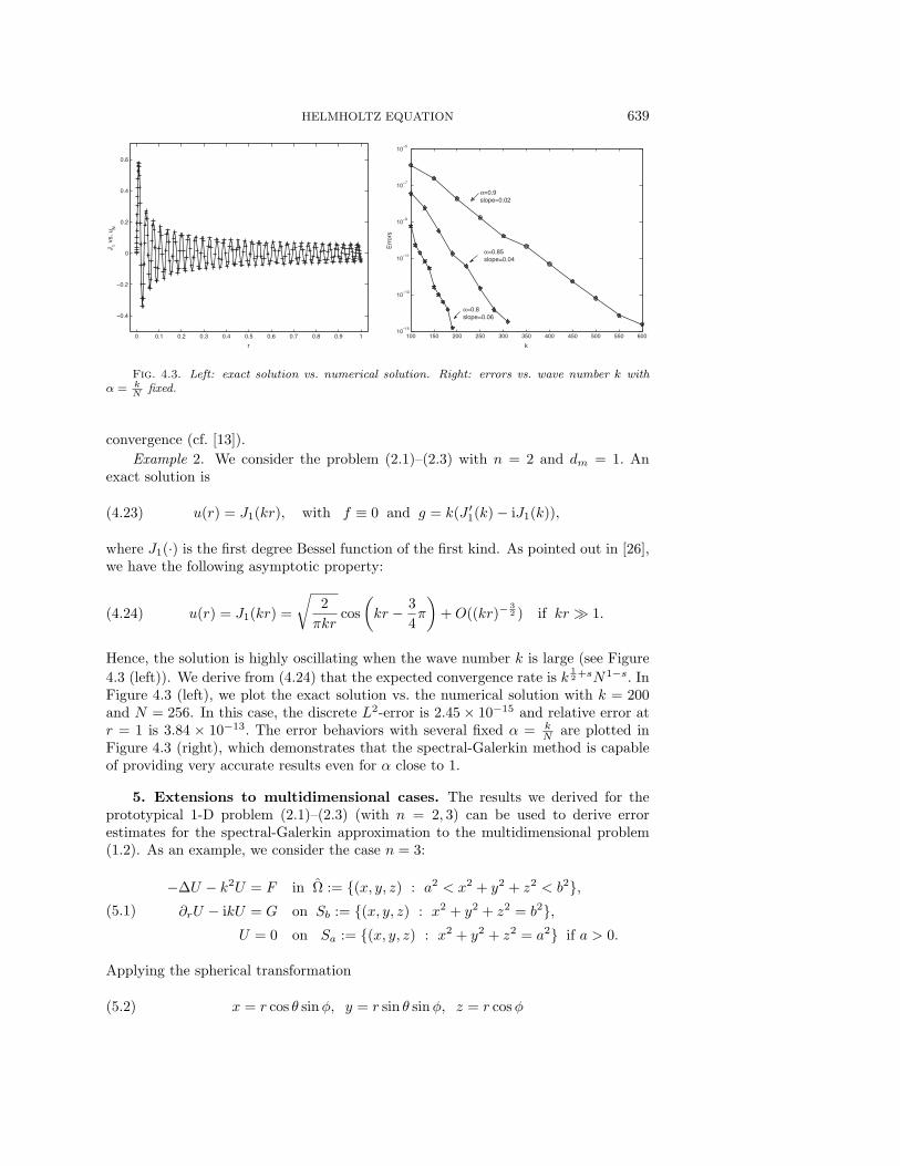
Fig. 4.3. Left: exact solution vs. numerical solution. Right: errors vs. wave number k withα = k

Nfixed.

convergence (cf. [13]).

Example 2. We consider the problem (2.1)–(2.3) with n = 2 and dm = 1. Anexact solution is

u(r) = J1(kr), with f ≡ 0 and g = k(J ′1(k) − iJ1(k)),(4.23)

where J1(·) is the first degree Bessel function of the first kind. As pointed out in [26],we have the following asymptotic property:

u(r) = J1(kr) =

√2

πkrcos

(kr − 3

4π

)+ O((kr)−

32 ) if kr � 1.(4.24)

Hence, the solution is highly oscillating when the wave number k is large (see Figure

4.3 (left)). We derive from (4.24) that the expected convergence rate is k12+sN1−s. In

Figure 4.3 (left), we plot the exact solution vs. the numerical solution with k = 200and N = 256. In this case, the discrete L2-error is 2.45 × 10−15 and relative error atr = 1 is 3.84 × 10−13. The error behaviors with several fixed α = k

N are plotted inFigure 4.3 (right), which demonstrates that the spectral-Galerkin method is capableof providing very accurate results even for α close to 1.

5. Extensions to multidimensional cases. The results we derived for theprototypical 1-D problem (2.1)–(2.3) (with n = 2, 3) can be used to derive errorestimates for the spectral-Galerkin approximation to the multidimensional problem(1.2). As an example, we consider the case n = 3:

−ΔU − k2U = F in Ω := {(x, y, z) : a2 < x2 + y2 + z2 < b2},∂rU − ikU = G on Sb := {(x, y, z) : x2 + y2 + z2 = b2},

U = 0 on Sa := {(x, y, z) : x2 + y2 + z2 = a2} if a > 0.

(5.1)

Applying the spherical transformation

x = r cos θ sinφ, y = r sin θ sinφ, z = r cosφ(5.2)


to (5.1) and setting u(r, θ, φ) = U(x, y, z), f(r, θ, φ) = F (x, y, z), g(θ, φ) = G(x, y, z),and S := [0, 2π) × [0, π), we obtain

−( ∂2

∂r2+

2

r

∂

∂r+

1

r2ΔS

)u− k2u = f in Ω := (a, b) × S,

∂ru− iku = g on Sb,

u = 0 on Sa if a > 0,

(5.3)

where ΔS is the Laplace–Beltrami operator (the Laplacian on the unit sphere S):

ΔS =1

sin2 φ

∂2

∂θ2+

cosφ

sinφ

∂

∂φ+

∂2

∂2φ.(5.4)

We recall that the spherical harmonic functions {Yl,m} are the eigenfunctions of theLaplace–Beltrami operator (see [25])

−ΔSYl,m(θ, φ) = m(m + 1)Yl,m(θ, φ)(5.5)

and are defined by

Yl,m(θ, φ) =

√(2m + 1)(m− l)!

4π(m + l)!eilθP l

m(cosφ), m ≥ |l| ≥ 0,

where P lm(x) is the associated Legendre functions given by

P lm(x) =

(−1)l

2mm!(1 − x2)

l2dm+l

dxm+1{(x2 − 1)m}.

The set of harmonic functions forms a complete orthonormal system in L2(S), i.e.,∫ 2π

0

∫ π

0

Yl,m(θ, φ)Yl′,m′(θ, φ) sinφdφdθ = δl,l′δm,m′ .(5.6)

Hence, for any function U(x, y, z) ∈ L2(Ω), the function u(r, θ, φ) = U(x, y, z) can beexpanded as

u =

∞∑|l|=0

∞∑m≥|l|

ulm(r)Yl,m(θ, φ), with ulm(r) =

∫S

u(r, θ, φ)Y l,m(θ, φ)dS,(5.7)

and we have

‖u‖2L2

ω2 (Ω) =

∞∑|l|=0

∞∑m≥|l|

‖ulm‖2ω2 = ‖U‖2

L2(Ω)(ω2 = r2).(5.8)

For a scalar function v on S, the gradient operator �∇S on the unit sphere isdefined by �∇Sv =

(1

sinφ∂θv, ∂φv). One can verify readily that

−(ΔSu, v)S = (�∇Su, �∇Sv)S ∀u, v ∈ D(ΔS),(5.9)

where D(ΔS) is the domain of the Laplace–Beltrami operator ΔS . In particular, as aconsequence of (5.5)–(5.9), we have

(�∇SYl,m, �∇SYl,m)S = m(m + 1), m ≥ |l| ≥ 0.(5.10)


Accordingly, we can define the Sobolev space on S:

H1(S) := {u : u is measurable on S and ‖u‖2H1(S) < ∞},

where ‖u‖H1(S) =(‖u‖2

L2(S) + ‖�∇Su‖2L2(S)

) 12 .

The variational formulation of (5.3) is to find u ∈ V := H1ω2(I;L2(S))∩L2(I;H1(S))

such that (ω2 = r2)

a(u, v) := (∂ru, ∂rv)ω2,Ω + (�∇Su, �∇Sv)Ω − k2(u, v)ω2,Ω

− ikb2(u(b, ·), v(b, ·))S = (f, v)ω2,Ω + b2(g, v(b, ·))S ∀v ∈ V.(5.11)

The spectral-Galerkin approximation of (5.11) is to find uMN ∈ VMN such that

a(uMN , v) = (f, v)ω2,Ω + b2(g, v(b, ·))S ∀v ∈ VMN ,(5.12)

where VMN := WM ×XN , and

WM := span{Yl,m : 0 ≤ |l| ≤ m ≤ M}, XN := {u ∈ PN : u(a) = 0 if a > 0}.

Hence, we can write

(u(r, θ, φ), f(r, θ, φ), g(θ, φ)) =∞∑

|l|=0

∞∑m≥|l|

(ulm(r), flm(r), glm)Yl,m(θ, φ);(5.13a)

uMN (r, θ, φ) =

M∑|l|=0

M∑m≥|l|

uNlm(r)Yl,m(θ, φ).(5.13b)

In order to describe the error bounds, we define a nonisotropic space Hsω2(I;Ht(S))

as follows:

Hsω2(I;Ht(S)) =

⎧⎨⎩u ∈ L2ω2(Ω) :

∞∑|l|=0

∞∑m≥|l|

mt(m + 1)t‖ulm‖2

Hs

ω2 (I)< +∞

⎫⎬⎭ ,(5.14)

where {ulm} are the expansion coefficients of u in terms of Yl,m as in (5.7). Thanks

to (5.10), we can define the norm on Hsω2(I;Ht(S)) by

‖u‖Hs

ω2 (I;Ht(S))=

⎛⎝ ∞∑|l|=0

∞∑m≥|l|

mt(m + 1)t‖ulm‖2

Hs

ω2 (I)

⎞⎠12

(5.15)

and its seminorm by replacing ‖ulm‖Hs

ω2 (I)with |ulm|

Hs

ω2 (I). In particular, L2

ω2(I;Ht(S))

= H0ω2(I;Ht(S)) and Hs

ω2(I;L2(S)) = Hsω2(I;H0(S)).

5.1. In a sphere (a = 0). Without loss of generality, we assume that b = 1. Inthis case, we can show that {ulm} (resp., {uN

lm}) satisfy the 1-D problem (2.5) (resp.,(3.1)) with n = 3 and f, g being replaced by flm and glm, respectively.

Theorem 5.1. Let u and uMN be, respectively, the solutions of (5.11) and (5.12),and denote e = u− uMN . Then if

u ∈ L2(I;Ht(S)) ∩H1ω2(I;Ht−1(S)) ∩ Hs

ω2(I;L2(S)), s, t ≥ 1, s, t ∈ N,(5.16)


we have

‖∂re‖L2

ω2 (Ω) + ‖�∇Se‖L2(Ω) + k‖e‖L2

ω2 (Ω)

� C∗

((M + M4k−4 + k2N−1)N1−s + M1−t(1 + kM−1)

),

(5.17)

where C∗ is a positive constant depending only on the seminorms of u in the spacesmentioned in (5.16).

Proof. Let elm(r) = ulm(r) − uNlm(r). We deduce from Theorem 3.2 that

‖∂relm‖L2

ω2 (I) +√dm‖elm‖L2(I) + k‖elm‖L2

ω2 (I)

�(1 +

√dm + d2

mk−4 + k2N−1)N1−s|elm|

Hs

ω2 (I),

(5.18)

where dm = m(m + 1). Therefore, by (5.6)–(5.10) and (5.13b)–(5.14),

‖∂re‖2L2

ω2 (Ω) + ‖�∇Se‖2L2(Ω) + k2‖e‖2

L2

ω2 (Ω)

=

M∑|l|=0

M∑m≥|l|

(‖∂relm‖2

L2

ω2 (I) + dm‖elm‖2L2(I) + k2‖elm‖2

L2

ω2 (I)

)

+

⎛⎝ ∞∑|l|=0

∞∑m>M

+

∞∑|l|>M

∞∑m≥|l|

⎞⎠(‖∂rulm‖2

L2

ω2 (I) + dm‖ulm‖2L2(I) + k2‖ulm‖2

L2

ω2 (I)

)

�(1 +

√dM + d2

Mk−4 + k2N−1)2

N2−2sM∑

|l|=0

M∑m≥|l|

|ulm|2Hs

ω2 (I)

+ d1−tM

∞∑|l|=0

∞∑m≥|l|

(dt−1m (‖∂rulm‖2

L2

ω2 (I) + dm‖ulm‖2L2(I) + k2‖ulm‖2

L2

ω2 (I)))

� (M + M4k−4 + k2N−1)2N2−2s|u|2Hs

ω2 (I;L2(S))

+ d1−tM

(|u|2H1

ω2 (I;Ht−1(S)) + |u|2L2(I;Ht(S)) + k2d−1m |u|2L2

ω2 (I;Ht(S))

),

which implies the desired result.

5.2. In a spherical shell (a > 0). In this case, {ulm} are the solutions of

Blm(ulm, v) = (flm, v)ω2 + b2glmv(b) ∀v ∈ X, 0 ≤ |l| ≤ m,(5.19)

where X := {u ∈ H1(I) : u(a) = 0}, and

Blm(u, v) := (∂ru, ∂rv)ω2 + dm(u, v) − k2(u, v)ω2 − ikb2u(b)v(b),(5.20)

with ω2 = r2, dm = m(m+1). The numerical approximations uNlm (0 ≤ |l| ≤ m, m =

0, 1, . . . ,M) are defined by

Blm(uNlm, vN ) = (flm, vN )ω2 + b2glmvN (b) ∀vN ∈ XN := X ∩ PN .(5.21)

Since ulm, (r−a)ulm ∈ X (resp., uNlm, (r−a)uN

lm ∈ XN ), we can use them as testfunctions in (5.19) (resp., (5.21)), and derive the following results using an argumentanalogous to that in the proof of Theorem 2.2.


Lemma 5.1. Let {ulm} and {uNlm} be, respectively, the solution of (5.19) and

(5.21). Then there exists ξ ∈ (a, b) such that for Cξ := (2 − 2aξ )−1, we have

‖∂rulm‖2L2

ω2 (I) + dm‖ulm‖2L2(I) + k2‖ulm‖2

L2

ω2 (I) � Cξb3(|glm|2 + b2‖flm‖2

L2

ω2 (I)),

‖∂ruNlm‖2

L2

ω2 (I) + dm‖uNlm‖2

L2(I) + k2‖uNlm‖2

L2

ω2 (I) � Cξb3(|glm|2 + b2‖flm‖2

L2

ω2 (I)).

The above a priori estimates allow us to perform the error analysis for the sphericalshell case. Similar to the case a = 0, we can prove the following.

Theorem 5.2. Let u and uMN be, respectively, the solutions of (5.11) and (5.12),and denote e = u− uMN . Then if

u ∈ L2((a, b);Ht(S)) ∩H1ω2((a, b);Ht−1(S)) ∩ Hs

ω2((a, b);L2(S)), s, t ≥ 1, s, t ∈ N,

there exists ξ ∈ (a, b) such that for Cξ := (2 − 2aξ )−1, we have

‖∂re‖L2

ω2 (Ω) + ‖�∇Se‖L2(Ω) + k‖e‖L2

ω2 (Ω)

� C∗b2(1 +

√Cξ)

((M + M4k−4 + k2N−1)N1−s + M1−t(1 + kM−1)

),

where C∗ is a positive constant depending only on the seminorms of u in the spacesmentioned in (5.16).

Remark 5.1. A similar procedure can be performed for the Helmholtz equation(1.2) in a 2-D axisymmetric domain (n = 2) by using a Fourier expansion in theθ-direction.

6. Concluding remarks. We presented in this paper a complete error analysisand an efficient numerical algorithm for the spectral-Galerkin approximation of theHelmholtz equation with high wave numbers in a 1-D domain as well as in multidi-mensional radial and spherical symmetric domains.

Our analysis is made possible by using two new arguments: (i) we employed a newprocedure advocated in [7] which allowed us to obtain sharp (in terms of k) a prioriestimates for both the continuous and discrete problems; (ii) we used new Jacobi andgeneralized Jacobi approximation results developed recently in [16, 24] which enabledus to derive optimal estimates for the cases n = 2, 3 which involve degenerate/singularcoefficients.

Unlike in most of the previous studies on the approximation of the Helmholtzequation with high wave numbers, our analysis does not rely on explicit knowledgeof continuous/discrete Green’s functions and is valid without any restriction on thewave number k and the discretization parameter N . Hence, it is possible to extend ourresults to more complex problems such as Helmholtz equations in an inhomogeneousmedium and to more complex domains through a suitable mapping or a domainperturbation technique.

Acknowledgment. The authors would like to thank Dr. Xiaobing Feng for manystimulating discussions and helpful suggestions.

REFERENCES

[1] I. M. Babuska and S. A. Sauter, Is the pollution effect of the FEM avoidable for the Helmholtzequation considering high wave numbers?, SIAM J. Numer. Anal., 34 (1997), pp. 2392–2423.


[2] J. P Berenger, A perfectly matched layer for the absorption of electromagnetic waves, J.Comput. Phys., 114 (1994), pp. 185–200.

[3] C. Bernardi and Y. Maday, Spectral methods, in Handbook of Numerical Analysis, Vol. 5(Part 2), P. G. Ciarlet and L. L. Lions, eds., North-Holland, Amsterdam, 1997, pp. 209–485.

[4] C. Canuto, M. Y. Hussaini, A. Quarteroni, and T. A. Zang, Spectral Methods in FluidDynamics, Springer-Verlag, New York, 1988.

[5] R. D. Ciskowski and C. A. Brebbia, Boundary Element Methods in Acoustics, Elsevier,London, 1991.

[6] P. Cummings, Analysis of Finite Element Based Numerical Methods for Acoustic Waves, Elas-tic Waves, and Fluid-Solid Iterations in the Frequency Domain, Ph.D. thesis, Universityof Tennessee, Knoxville, 2001.

[7] P. Cummings and X. B. Feng, Sharp regularity coefficient estimates for complex-valued acous-tic and elastic Helmholtz equations, Math. Models Methods Appl. Sci., to appear.

[8] J. Douglas, J. E. Santos, D. Sheen, and L. S. Bennethum, Frequency domain treatment ofone-dimensional scalar waves, Math. Models Methods Appl. Sci., 3 (1993), pp. 171–194.

[9] J. Douglas, Jr., D. Sheen, and J. E. Santos, Approximation of scalar waves in the space-frequency domain, Math. Models Methods Appl. Sci., 4 (1994), pp. 509–531.

[10] X. Feng and D. Sheen, An elliptic regularity coefficient estimate for a problem arising from afrequency domain treatment of waves, Trans. Amer. Math. Soc., 346 (1994), pp. 475–487.

[11] K. Gerdes and L. Demkowicz, Solution of 3D-Laplace and Helmholtz equations in exteriordomains using hp-infinite elements, Comput. Methods Appl. Mech. Engrg., 137 (1996),pp. 239–273.

[12] K. Gerdes and F. Ihlenburg, On the pollution effect in FE solutions of the 3D-Helmholtzequation, Comput. Methods Appl. Mech. Engrg., 170 (1999), pp. 155–172.

[13] D. Gottlieb and S. A. Orszag, Numerical Analysis of Spectral Methods: Theory and Appli-cations, CBMS-NSF Regional Conf. Ser. in Appl. Math. 26, SIAM, Philadelphia, 1977.

[14] M. J. Grote and J. B. Keller, On non-reflecting boundary conditions, J. Comput. Phys.,122 (1995), pp. 231–243.

[15] B. Y. Guo and L. L. Wang, Jacobi interpolation approximations and their applications tosingular differential equations, Adv. Comput. Math., 14 (2001), pp. 227–276.

[16] B. Y. Guo and L. L. Wang, Jacobi approximations in non-uniformly Jacobi-weighted Sobolevspaces, J. Approx. Theory, 128 (2004), pp. 1–41.

[17] G. H. Hardy, J. E. Littlewood, and G. Polya, Inequalities, Cambridge University Press,Cambridge, UK, 1952.

[18] F. Ihlenburg and I. Babuska, Finite element solution of the Helmholtz equation with highwave number, Part I: The h-version of FEM, Comput. Math. Appl., 30 (1995), pp. 9–37.

[19] F. Ihlenburg and I. Babuska, Finite element solution of the Helmholtz equation with highwave number. Part II: The h-p version of the FEM, SIAM J. Numer. Anal., 34 (1997), pp.315–358.

[20] F. John, Partial Differential Equations, 4th ed., Springer-Verlag, New York, 1982.[21] A. H. Schatz, An observation concerning Ritz-Galerkin methods with indefinite bilinear forms,

Math. Comp., 28 (1974), pp. 959–962.[22] J. Shen, Efficient spectral-Galerkin method. I. Direct solvers for second- and fourth-order

equations using Legendre polynomials, SIAM J. Sci. Comput., 15 (1994), pp. 1489–1505.[23] J. Shen, Efficient spectral-Galerkin methods III: Polar and cylindrical geometries, SIAM J.

Sci. Comput., 18 (1997), pp. 1583–1604.[24] J. Shen and L. L. Wang, Error analysis for mapped Jacobi spectral methods, J. Sci. Comput.,

to appear.[25] I. N. Sneddon, Special Functions of Mathematical Physics and Chemistry, 3rd ed., Longman,

New York, 1980.[26] G. N. Watson, A Treatise of the Theory of Bessel Functions, 2nd ed., Cambridge University

Press, Cambridge, UK, 1966.

audit of douglas county assessor fy 2007/2008 #05 douglas county

Documents