Attribute systems and plumbing diagrams

Andrew Seniuk Robin Cockett

March 26, 2007

1 Introduction

The purpose of these notes is to provide a gentle introduction to attribute systems using plumbingdiagrams. These notes were developed to supplement the course material of CPSC411, Introduc-tion to Compilers, and employ a graphical representation of attribute systems, called “plumbingdiagrams”, in order to represent, particularly, the semantic analysis stage of a simple compiler.Attribute systems are usually associated with a context free grammar, however, in these notes andin the class we associate them more generally with datatypes and view them as a way of expressinga computation on a datatype. This makes them more generally applicable and provides those whoget to understand what they are about a powerful program development tool.

2 What is an attribute system?

From a pragmatic viewpoint, an attribute system is a specification of a program. Given a datatype,an attribute is some computable characteristic (e.g. numeric value, type, or space requirement) forwhich a program is wanted. An attribute system indicates how the attribute is calculated, andusually this involves showing how it is computed from other attributes. A given datatype mayhave many different attribute systems associated with it, each one for computing correspondingattributes. Once you have a valid attribute system it can be used as a template to write actualcode which, if the translation is done correctly, is guaranteed to work.

Attribute systems at first sight are rather complex things so we shall approach them from aninformal point of view to start with. Plumbing diagrams such as the sample shown in Figure 1provide a visual representation of the complexities of attribute systems and will be used throughout

1

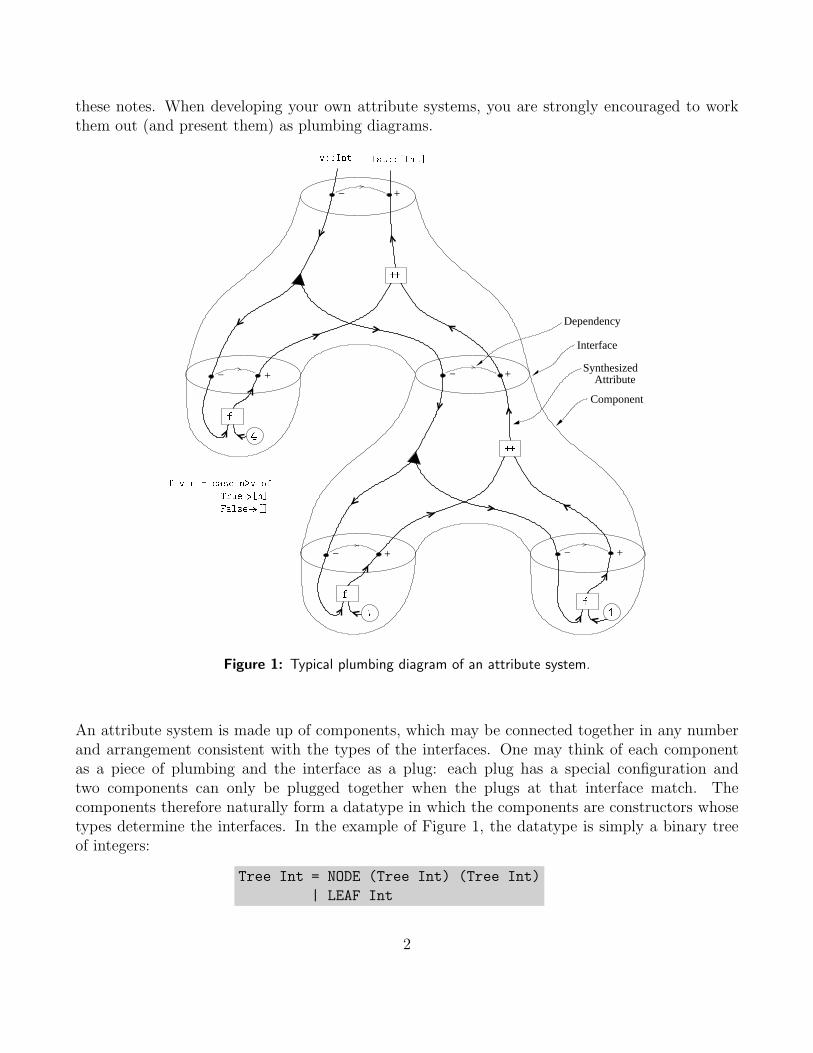
these notes. When developing your own attribute systems, you are strongly encouraged to workthem out (and present them) as plumbing diagrams.

− +

− +

− +

−

− +

Synthesized

Component

Attribute+

Dependency

Interface

f v n = ase n>v ofTrue-->[n℄4

7 1ff

f ++

++

False-->[℄

v::Int lst::[Int℄

Figure 1: Typical plumbing diagram of an attribute system.

An attribute system is made up of components, which may be connected together in any numberand arrangement consistent with the types of the interfaces. One may think of each componentas a piece of plumbing and the interface as a plug: each plug has a special configuration andtwo components can only be plugged together when the plugs at that interface match. Thecomponents therefore naturally form a datatype in which the components are constructors whosetypes determine the interfaces. In the example of Figure 1, the datatype is simply a binary treeof integers:

Tree Int = NODE (Tree Int) (Tree Int)

| LEAF Int

2

This datatype has two constructors, and so there are two kinds of components possible in attributesystems for this datatype, one for NODE and one for LEAF. In our particular example, the attributesystem computes the list of integers from the leaves of the tree (in left to right order) which havevalue greater than a threshold v.

− +

− +

− +

− +++ LEAFNODE

Nflst

lst1

v lst

v

v2 lst2v1

Figure 2: The two kinds of components possible in our attribute system of Figure 1.

The NODE component performs two computations (also called equations in the textbook):

• The integer v is copied into v1 and v2.

• Lists lst1 and lst2 are concatenated to give lst.

The LEAF component performs one computation: It applies the function f to the inherited attributev and the constant integer N, which returns a list either empty or singleton.

f v n = case n>v of

True-->[n]

False-->[]

Bear in mind that, while the computation in this example is very basic, it’s the idea of an attributesystem which is the point. Attribute systems provide us with a powerful tool for organizing andwriting correct code in cases where the computations involved are monstrously complex.

However, there is a danger of things going awry. Even though each component represents a sensiblecomputation, if precautions aren’t taken it may happen that a connected assemblage representsa nonsensical computation. This is illustrated in Figure 3, to which we’ll return for a thoroughanalysis in Section 5.

Since there is no limit to the number of components which can be assembled, and problemsmight only become apparent in some very large assemblies, checking the validity of an attribute

3

4

− − + ++

− +

−

β

α

− − + ++

− +

−

4β

α

Plumbing diagram exhibiting circular dependencies. This one represents a valid computation.

Figure 3: Depending on how components are connected up, cycles of dependencies may be possible; compo-nent definitions which can give rise to such constructions do not constitute a valid attribute system.

system cannot be reduced to checking all possibilities. This is where some theory becomes useful:in particular conditions regarding circularity will come to the rescue, as we’ll see after definingattribute systems more formally.

3 Formal definition of an Attribute System

Here is the definition of an attribute system that we shall use. This is sometimes called a “stronglynon-circular” attribute system in compiler texts.

An attribute system consists of:

1. A mutually recursive collection of inductive datatypes (or a context free grammar).

2. For each type (non-terminal) a set of attributes which are labelled as either inherited (−) orsynthesized (+).

3. For each type (non-terminal) a dependency specification for each synthesized attribute uponthe inherited attributes.

4. With each constructor (production), a function for calculating:

(a) each synthesized parent attribute, and

4

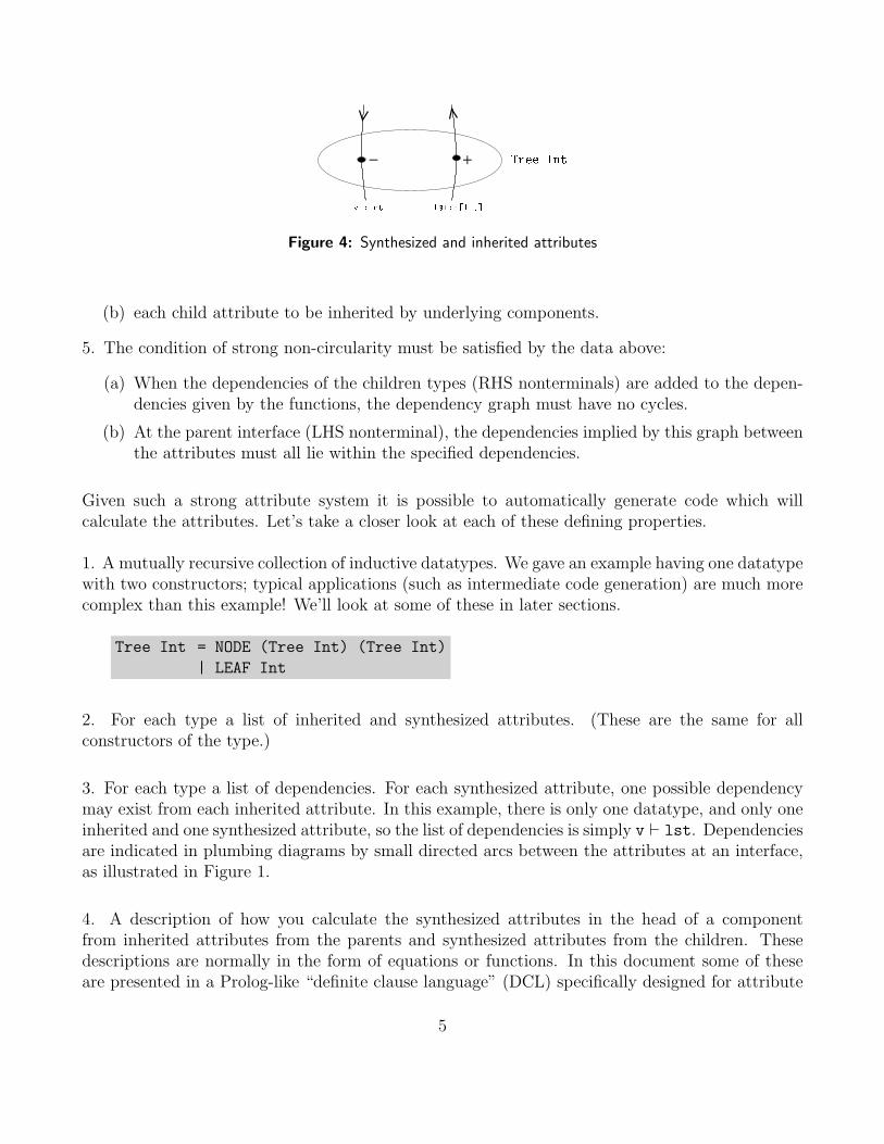
− + Tree Intlst::[Int℄v::Int

Figure 4: Synthesized and inherited attributes

(b) each child attribute to be inherited by underlying components.

5. The condition of strong non-circularity must be satisfied by the data above:

(a) When the dependencies of the children types (RHS nonterminals) are added to the depen-dencies given by the functions, the dependency graph must have no cycles.

(b) At the parent interface (LHS nonterminal), the dependencies implied by this graph betweenthe attributes must all lie within the specified dependencies.

Given such a strong attribute system it is possible to automatically generate code which willcalculate the attributes. Let’s take a closer look at each of these defining properties.

1. A mutually recursive collection of inductive datatypes. We gave an example having one datatypewith two constructors; typical applications (such as intermediate code generation) are much morecomplex than this example! We’ll look at some of these in later sections.

Tree Int = NODE (Tree Int) (Tree Int)

| LEAF Int

2. For each type a list of inherited and synthesized attributes. (These are the same for allconstructors of the type.)

3. For each type a list of dependencies. For each synthesized attribute, one possible dependencymay exist from each inherited attribute. In this example, there is only one datatype, and only oneinherited and one synthesized attribute, so the list of dependencies is simply v ` lst. Dependenciesare indicated in plumbing diagrams by small directed arcs between the attributes at an interface,as illustrated in Figure 1.

4. A description of how you calculate the synthesized attributes in the head of a componentfrom inherited attributes from the parents and synthesized attributes from the children. Thesedescriptions are normally in the form of equations or functions. In this document some of theseare presented in a Prolog-like “definite clause language” (DCL) specifically designed for attribute

5

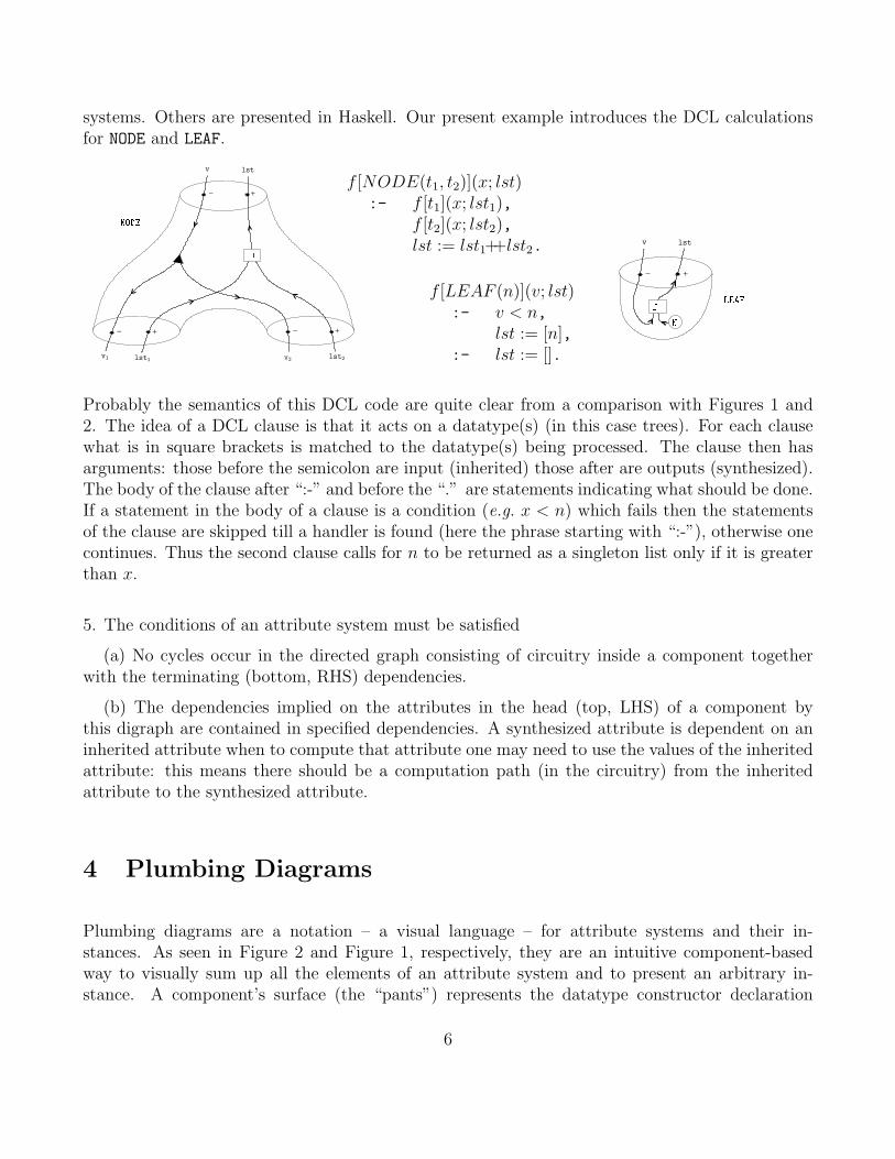
systems. Others are presented in Haskell. Our present example introduces the DCL calculationsfor NODE and LEAF.

− +

− +

− +

++

lst1

v lst

v2 lst2v1

NODEf [NODE(t1, t2)](x; lst)

:- f [t1](x; lst1),f [t2](x; lst2),lst := lst1++lst2.

f [LEAF (n)](v; lst):- v < n,

lst := [n],:- lst := [].

− + LEAFNflstv

Probably the semantics of this DCL code are quite clear from a comparison with Figures 1 and2. The idea of a DCL clause is that it acts on a datatype(s) (in this case trees). For each clausewhat is in square brackets is matched to the datatype(s) being processed. The clause then hasarguments: those before the semicolon are input (inherited) those after are outputs (synthesized).The body of the clause after “:-” and before the “.” are statements indicating what should be done.If a statement in the body of a clause is a condition (e.g. x < n) which fails then the statementsof the clause are skipped till a handler is found (here the phrase starting with “:-”), otherwise onecontinues. Thus the second clause calls for n to be returned as a singleton list only if it is greaterthan x.

5. The conditions of an attribute system must be satisfied

(a) No cycles occur in the directed graph consisting of circuitry inside a component togetherwith the terminating (bottom, RHS) dependencies.

(b) The dependencies implied on the attributes in the head (top, LHS) of a component bythis digraph are contained in specified dependencies. A synthesized attribute is dependent on aninherited attribute when to compute that attribute one may need to use the values of the inheritedattribute: this means there should be a computation path (in the circuitry) from the inheritedattribute to the synthesized attribute.

4 Plumbing Diagrams

Plumbing diagrams are a notation – a visual language – for attribute systems and their in-stances. As seen in Figure 2 and Figure 1, respectively, they are an intuitive component-basedway to visually sum up all the elements of an attribute system and to present an arbitrary in-stance. A component’s surface (the “pants”) represents the datatype constructor declaration

6

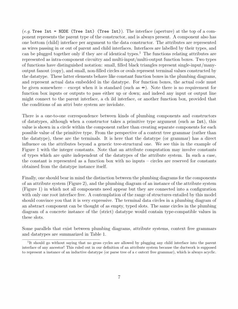
(e.g. Tree Int = NODE (Tree Int) (Tree Int)). The interface (aperture) at the top of a com-ponent represents the parent type of the constructor, and is always present. A component also hasone bottom (child) interface per argument to the data constructor. The attributes are representedas wires passing in or out of parent and child interfaces. Interfaces are labelled by their types, andcan be plugged together only if they are of identical types.1 The functions relating attributes arerepresented as intra-component circuitry and multi-input/multi-output function boxes. Two typesof functions have distinguished notation: small, filled black triangles represent single-input/many-output fanout (copy), and small, non-filled circles or ovals represent terminal values constructed bythe datatype. These latter elements behave like constant function boxes in the plumbing diagrams,and represent actual data embedded in the datatype. For function boxes, the actual code mustbe given somewhere – except when it is standard (such as ++). Note there is no requirement forfunction box inputs or outputs to pass either up or down; and indeed any input or output linemight connect to the parent interface, a ch ild interface, or another function box, provided thatthe conditions of an attri bute system are inviolate.

There is a one-to-one correspondence between kinds of plumbing components and constructorsof datatypes, although when a constructor takes a primitive type argument (such as Int), thisvalue is shown in a circle within the component rather than creating separate components for eachpossible value of the primitive type. From the perspective of a context tree grammar (rather thanthe datatype), these are the terminals. It is here that the datatype (or grammar) has a directinfluence on the attributes beyond a generic tree-structural one. We see this in the example ofFigure 1 with the integer constants. Note that an attribute computation may involve constantsof types which are quite independent of the datatypes of the attribute system. In such a case,the constant is represented as a function box with no inputs – circles are reserved for constantsobtained from the datatype instance itself.

Finally, one should bear in mind the distinction between the plumbing diagrams for the componentsof an attribute system (Figure 2), and the plumbing diagram of an instance of the attribute system(Figure 1) in which not all components need appear but they are connected into a configurationwith only one root interface free. A contemplation of the range of structures entailed by this modelshould convince you that it is very expressive. The terminal data circles in a plumbing diagram ofan abstract component can be thought of as empty, typed slots. The same circles in the plumbingdiagram of a concrete instance of the (strict) datatype would contain type-compatible values inthese slots.

Some parallels that exist between plumbing diagrams, attribute systems, context free grammarsand datatypes are summarized in Table 1.

1It should go without saying that no gross cycles are allowed by plugging any child interface into the parentinterface of any ancestor! This ruled out in our definition of an attribute system because the ductwork is supposedto represent a instance of an inductive datatype (or parse tree of a c ontext free grammar), which is always acyclic.

7

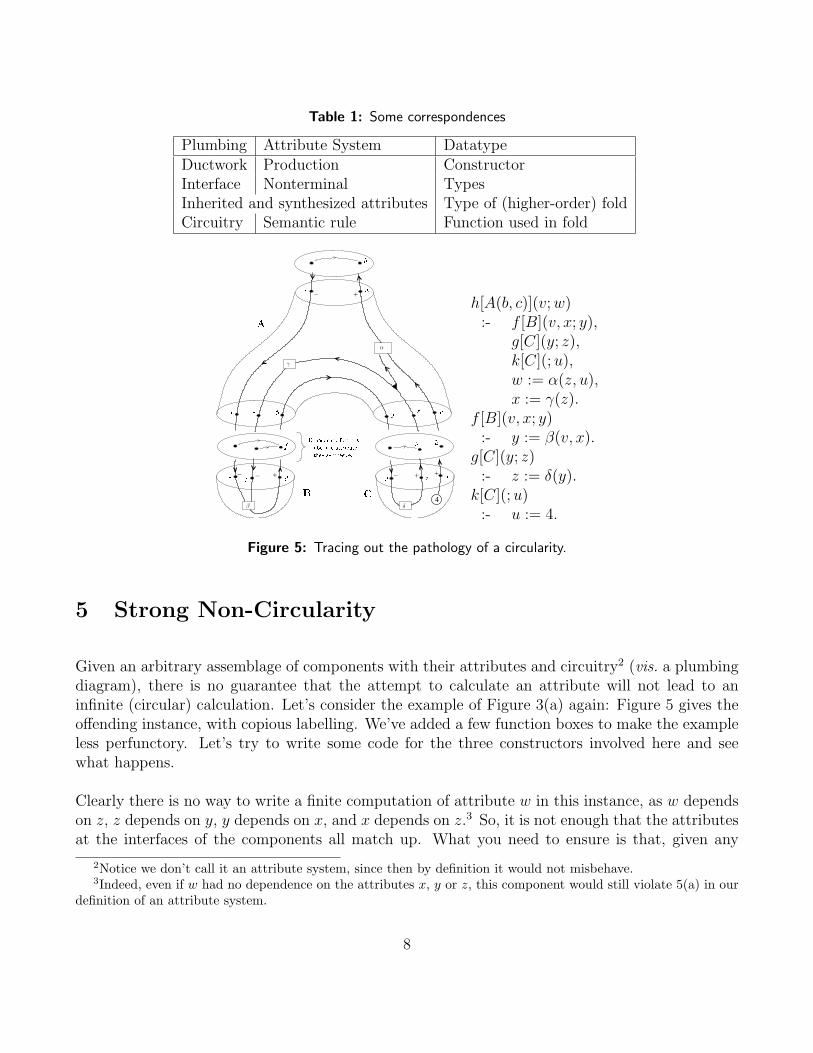
Table 1: Some correspondences

Plumbing Attribute System DatatypeDuctwork Production ConstructorInterface Nonterminal TypesInherited and synthesized attributes Type of (higher-order) foldCircuitry Semantic rule Function used in fold

4

− − + ++

− +

−

Dependen y fu tionsthey synthesize.label the attributeβ δ

gv x y uy u

A

CB

γ

α

zk

zfyv x

y

hv wh[A(b, c)](v; w)

:- f [B](v, x; y),g[C](y; z),k[C](; u),w := α(z, u),x := γ(z).

f [B](v, x; y):- y := β(v, x).

g[C](y; z):- z := δ(y).

k[C](; u):- u := 4.

Figure 5: Tracing out the pathology of a circularity.

5 Strong Non-Circularity

Given an arbitrary assemblage of components with their attributes and circuitry2 (vis. a plumbingdiagram), there is no guarantee that the attempt to calculate an attribute will not lead to aninfinite (circular) calculation. Let’s consider the example of Figure 3(a) again: Figure 5 gives theoffending instance, with copious labelling. We’ve added a few function boxes to make the exampleless perfunctory. Let’s try to write some code for the three constructors involved here and seewhat happens.

Clearly there is no way to write a finite computation of attribute w in this instance, as w dependson z, z depends on y, y depends on x, and x depends on z.3 So, it is not enough that the attributesat the interfaces of the components all match up. What you need to ensure is that, given any

2Notice we don’t call it an attribute system, since then by definition it would not misbehave.3Indeed, even if w had no dependence on the attributes x, y or z, this component would still violate 5(a) in our

definition of an attribute system.

8

− + +−

+−

−+

Figure 6: Violation of condition 5(b) for strong non-circularity: There are two implied dependencies on theparent interface which are not part of the specified dependencies, presuming that all specified dependenciesare shown.

instance of the datatype (parse tree) and any attribute, it is always possible to calculate it. Thismeans that whatever tree you build, the calculations associated with the attributes must neverinvolve a cycle. Given that there may be infinitely many possible such trees you should note thatthis is not something that can be simply checked by examining the possibilities!

It is possible to determine whether a “general” attribute system, as above, is non-circular but thealgorithm is exponential.4 However, there is a stronger notion, often called strong non-circularity ,which is easy to check and is, in fact, the condition which is used in practise. The two requirementsfor strong non-circularity were given by 5(a) and 5(b) in the definition of an attribute system. 5(a)prevents explicit circular calculations within a component, and 5(b) checks that the specifieddependencies include all the implied dependencies which result from the circuitry. A failure of5(a) indicates an error in your logical plan! Failure of 5(b) is more complicated: it may meanyou need to add some more specified dependencies to your attribute system (i.e. your choices instep 3 of the definition were not sufficiently complete), after which 5(a) needs to be checked againand, considering that the graph will now have additional arrows, the risk of a failure of condition5(a) will increased. The nice thing about strong non-circularity is that one can check it merely berunning these checks on each component in isolation. However, there do exist computable attributesystems which violate strong non-circularity – we are only assured that every strongly non-circularattribute system is computable, not that such systems describe every possible computation.

Given the specified dependencies on the children nonterminals (RHS or argument types) and thedependencies implied by the equations it is possible to generate for each production (or constructor)a little directed graph where an arrow indicates a dependency. If this graph has no cycles andthe implied dependencies on the parent are always contained within the specified dependencies for

4See the text: in fact this check relies on determining all the possible dependencies which is what makes itexponential.

9

that nonterminal (or type) then the attribute system will be non-circular.

The proof of this is as follows: suppose there is a (parse) tree with a cycle of dependencies thenthere is a topmost nonterminal (type) through which this cycle passes. The cycle below thisnonterminal (type) produces a dependency −N.a → +N.b. This must be one of the specifieddependencies (a simple inductive argument on the underlying tree). But the cycle is formed by adependency +N.b → −N.a above the nonterminal which produces an instantaneous cycle in thecalculation of the graph for that production (constructor).

This means you can write the code!

6 Applications

6.1 Code to check that numbers are well-formed

As a one-paragraph crash course in the definite clause language (DCL), consider some examplecode

base num [bn(N, B)](; z):- base[B](; b),

num[N ](b; z).

dig [n](b; m):- n < b,

m := n.

Each group of statements corresponding to a constructor is a ‘clause’. The phrases of each clausecan contain guards which must evaluate to true in order to continue the normal evaluation ofclause. If a guard fails one looks for an exception handler. In Haskell this could be modelled withan exception monad like Maybe or Error from the Haskell Standard Prelude. For example, dig[n](b; n) = n < b. fails unless n < b in which case it synthesizes n.

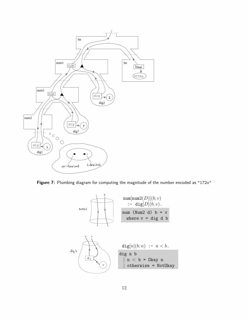
We’re now ready to tackle the complete problem. Consider the following grammar for non-negativeintegers, of base either octal or decimal. The plumbing diagram in Figure 7 illustrates a possibleparse relative to this grammar, along with attribute calculations for the value of the number. Notethat this value is a magnitude and has no particular base associated with it – the base is a featureof the representation of the number, not a feature of its value.

10

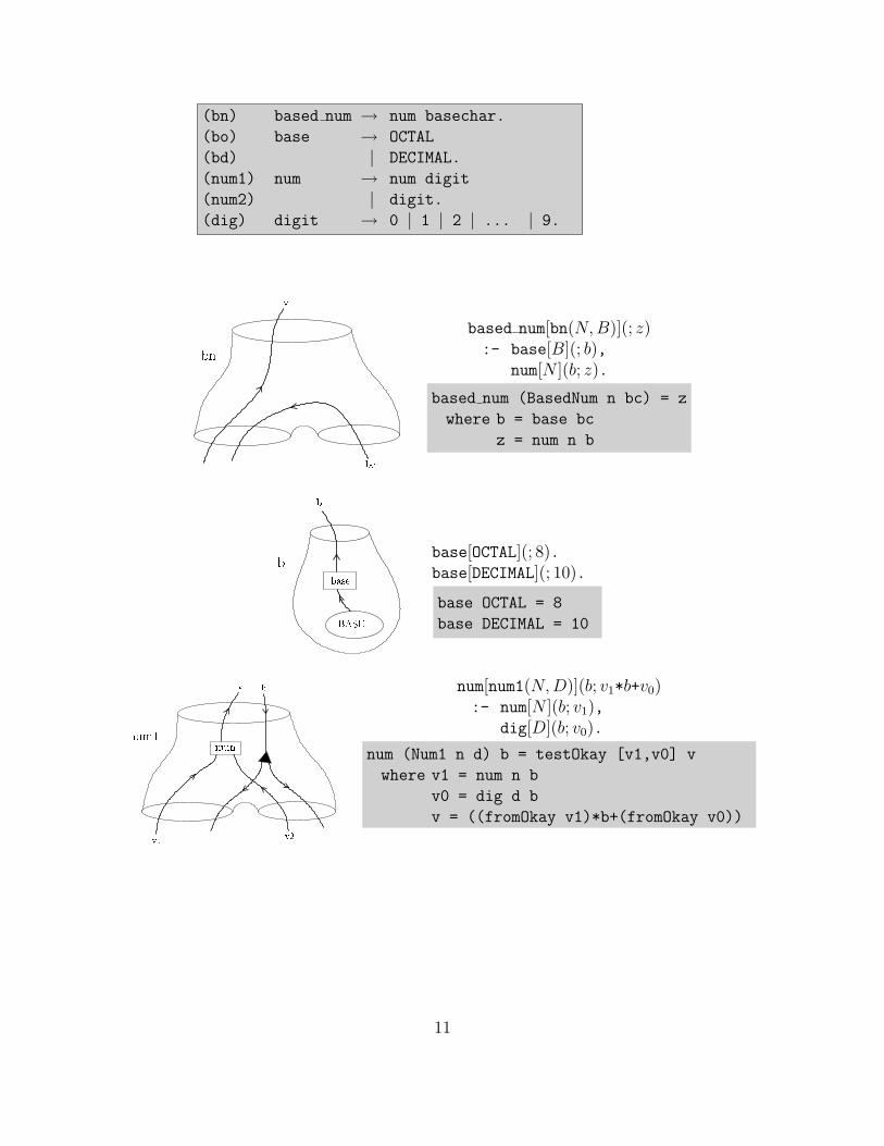
(bn) based num → num basechar.

(bo) base → OCTAL

(bd) | DECIMAL.

(num1) num → num digit

(num2) | digit.

(dig) digit → 0 | 1 | 2 | ... | 9.

b

vbn based num[bn(N, B)](; z)

:- base[B](; b),num[N ](b; z).

based num (BasedNum n bc) = z

where b = base bc

z = num n b

BASEbaseb

b base[OCTAL](; 8).base[DECIMAL](; 10).

base OCTAL = 8

base DECIMAL = 10

numv1 v2

v bnum1

num[num1(N, D)](b; v1*b+v0):- num[N ](b; v1),

dig[D](b; v0).

num (Num1 n d) b = testOkay [v1,v0] v

where v1 = num n b

v0 = dig d b

v = ((fromOkay v1)*b+(fromOkay v0))

11

num1

num1

bn

bo

num2

dig1

dig7

dig2

num

numdig

dig

dig

OCTAL

+ -synthesized inherited17

2base

Figure 7: Plumbing diagram for computing the magnitude of the number encoded as "172o"bvnum2 num[num2(D)](b; v)

:- dig[D](b; v).

num (Num2 d) b = v

where v = dig d b

Ndigv b

digN dig[n](b; n) :- n < b.

dig n b

| n < b = Okay n

| otherwise = NotOkay

12

The code for this computation is expressed in both DCL and Haskell. For more information aboutthe Okay monad, you can refer to Appendix A, but roughly speaking, testOkay returns its secondargument (wrapped in an Okay) if every element of the list in the first argument is Okay, andreturns NotOkay otherwise.

6.2 A simple symbol table, and let expressions

The symbol table is a list of identifiers [x1, y1, x2, ...] supporting two operations: insertion, andmembership test.

insert(x,st;st’) to add an element to the front of the list.

member(x,st;) to check for membership in the list.

Consider the following simple expression grammar.5

exp → exp + exp

| (exp)

| ID

| NUM

| LET decls IN exp.

decls → decls , dec

| dec.

dec → ID = exp.

data exp = ADD(exp,exp)

| PAR(exp)

| ID(string)

| NUM(int)

| LET(decls,exp)

data decls = MANY(decls,dec)

| ONE(dec)

data dec = DEC(string,exp)

Grammar Syntax Tree

A typical expression is then

let y = 22 in

( let x = 4+y , z=7+y in x+z+y )

Given an expression and a symbol table, how does one check whether the expression is well-formed?It is well-formed if the values of variables are all declared before they are used. Thus the above iswell formed. Here is a summary of the scoping rules:

• The usual scope rule: that is if v is declared in D then v can be used in the term t in let D

in t).

5This grammar is both left-recursive and ambiguous! However, we shall just use the parse trees as the basis foran attribute grammar; the technicalities of the parse are immaterial here.

13

• Simultaneous declaration semantics: a declaration can only use variable which are alreadydeclared and these do not include the variables in the same declaration list. Thus, let x=3,

y=x in 2y is not legal.

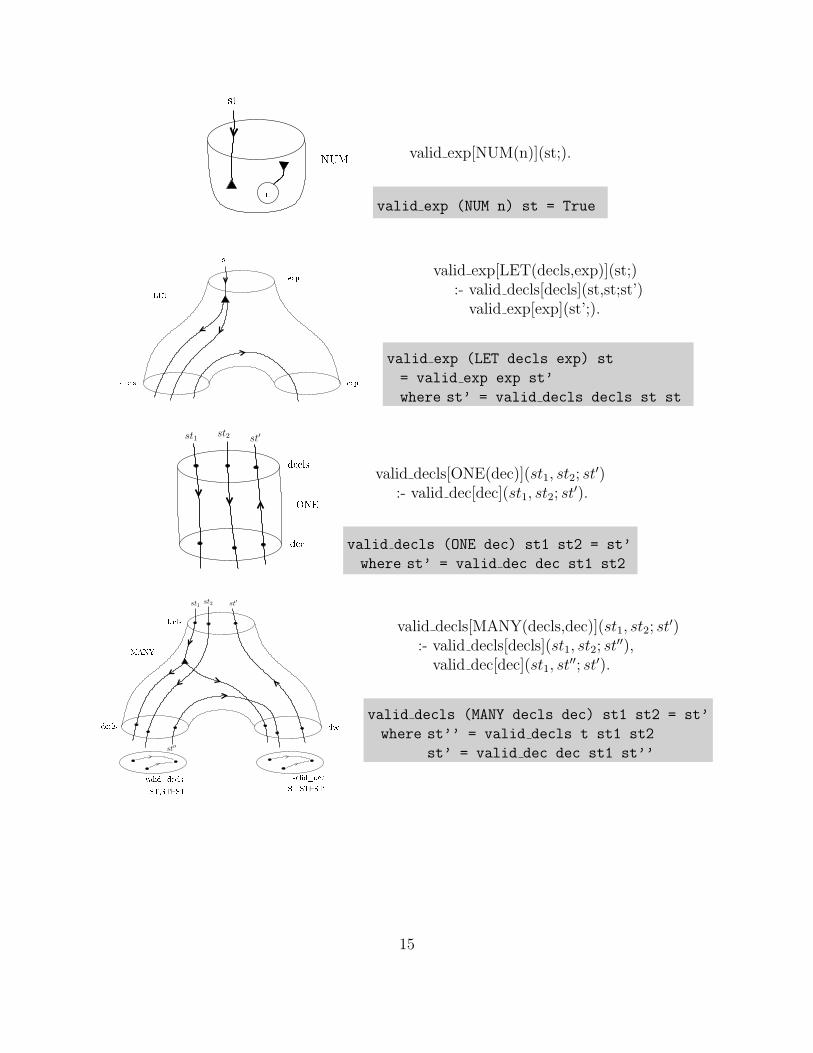
In this attribute system if a retrieveal from the sytmbol table (which is a membership test) fails,the whole expression is immediately deemed to be ill-formed. The following are the componentsof an attribute system implementing this solution, with the plumbing diagram for an exampleexpression given in Figure 6.2. For the last three, the first symbol table is for checking expressions,and the second symbol table is for collecting declarations.

st

exp

exp

expADD valid exp[ADD(t1, t2)](st;)

:- valid exp[t1](st;),valid exp[t2](st;).

valid exp (ADD t1 t2) st =

valid exp t1 st

valid exp t2 ststPAR valid exp[PAR(t)](st;)

:- valid exp[t](st;).

valid exp (PAR t) st =

valid exp t st

memberstrst

ID valid exp[ID(str)](st;):- member(str,st).

valid exp (ID str) st =

member str st

14

nst

NUM valid exp[NUM(n)](st;).

valid exp (NUM n) st = True

st

de ls expLET exp valid exp[LET(decls,exp)](st;)

:- valid decls[decls](st,st;st’)valid exp[exp](st’;).

valid exp (LET decls exp) st

= valid exp exp st’

where st’ = valid decls decls st st

de lsONEde st1

st2st

′

valid decls[ONE(dec)](st1, st2; st′)

:- valid dec[dec](st1, st2; st′).

valid decls (ONE dec) st1 st2 = st’

where st’ = valid dec dec st1 st2

de valid_de lsST,ST⊢ST valid_de ST,ST⊢ST

de lsMANYde ls

st1st2 st

′

st′′

valid decls[MANY(decls,dec)](st1, st2; st′)

:- valid decls[decls](st1, st2; st′′),

valid dec[dec](st1, st′′; st′).

valid decls (MANY decls dec) st1 st2 = st’

where st’’ = valid decls t st1 st2

st’ = valid dec dec st1 st’’

15

inserty

x 3member

memberx7

st

ADDNUMID

IDADD

NUM

DECONELET

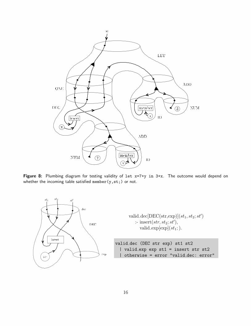
Figure 8: Plumbing diagram for testing validity of let x=7+y in 3+x. The outcome would depend onwhether the incoming table satisfied member(y,st;) or not.

strinsert

de

expDEC

st1st2

st′

valid dec[DEC(str,exp)](st1, st2; st′)

:- insert(str, st2; st′),

valid exp[exp](st1; ).

valid dec (DEC str exp) st1 st2

| valid exp exp st1 = insert str st2

| otherwise = error "valid dec: error"

16

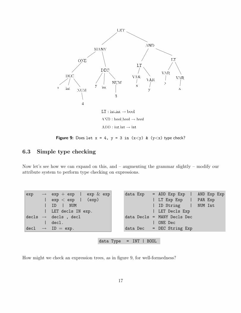
MANYONEDEC DECx int NUM4 y int NUM3 VAR VAR VAR VARLT LTANDLET

x y xyLT : int,int → boolAND : bool,bool → boolADD : int,int → int

Figure 9: Does let x = 4, y = 3 in (x<y) & (y<x) type check?

6.3 Simple type checking

Now let’s see how we can expand on this, and – augmenting the grammar slightly – modify ourattribute system to perform type checking on expressions.

exp → exp + exp | exp & exp

| exp < exp | (exp)

| ID | NUM

| LET decls IN exp.

decls → decls , decl

| decl.

decl → ID = exp.

data Exp = ADD Exp Exp | AND Exp Exp

| LT Exp Exp | PAR Exp

| ID String | NUM Int

| LET Decls Exp

data Decls = MANY Decls Dec

| ONE Dec

data Dec = DEC String Exp

data Type = INT | BOOL

How might we check an expression trees, as in figure 9, for well-formedness?

17

expstring

he k_addexp

exp

st typeADD VAR

exp st type

st st

retrieve

type1 type

2

type check exp[ADD(t1, t2)](st;type):- type check exp[t1](st;type1)

type check exp[t2](st;type2)

check add(type1, type2; type).

type check exp[VAR(str)](st;type)

:- retrieve(str;type).

check add(t1, t2;INT):- t1 =INT,t2 =INT.

We need a symbol table as before ... but it is slightly more complex as it needs to hold typeinformation for each declared variable:

[(x, int), (y, bool), ...]

As before, inserting adds the decalation to the front of list. A retrieval, given a string, will returna type or fail (recall the the example above retrieval merely succeeded or failed).

retrieve(x,[(x,int),(y,bool)];INT) Succeeds and returns the type INT.retrieve(z,[(x,int),(y,bool)]; ) Fails.

6.4 “Dance of the symbol table”

If the function types are also stored in the symbol table, what would the code look like if we wantedto build an intermediate representation. It actually means that we must thread the symbol tablealmost twice round the code: first to pick up the function names and types and second to handlethe variable declarations.

The rest of these notes will sketch the salient aspects of defining an attribute system to calculateintermediate representation data for programs in a simple programming language. We’ll begin

18

st

type irst he k_add ADD

st type1

ir1 ir2type2

Figure 10: Returning a type and an intermediate representation for expressions

with a simple expression grammar, then introduce let-style local declarations, then types andtype-checking, and finally scoped function declarations permitting in-block forward references. Wedrop the monadic Haskell exception model for the sake of more lucid code, with the understandingthat exception handling can be restored essentially mechanically.

collects[decls](table;table′) :-genfuns[decls](table′;ir fun),genstmts[stmts](table′;ir stmts),ir := (ir fun,ir stmts).

ir decls stmts = (ir fun,ir stmts)

where table’ = collects decls table

ir fun = genfuns decls table’

ir stmts = genstmts stmts table’

collects[decl::decls](table;table′′) : −collect[decl](table;table′),collects[decl](table′;table′′). collects (decl:decls) table

= collects decls $ collect decl table

19

tablesymbol ir for

block

newtable functions

ir forir forstmts

block

collects genstmtsgenfunsdecls stmts

block

BLOCK\x y-->(x,y)

Figure 11: The symbol table dance for blocks

olle ts genfuns

olle t genfun olle ts genfunsde lsde l

de ls\h t-->h:t

Figure 12: Tne symbol table dance for declarations

20

genfuns[decl::decls](table;ir fun::ir funs) : −genfun[decl](table;ir fun),genfuns[decls](table;ir funs).

genfuns[nil](table;nil).

genfuns [] table = []

genfuns (decl:decls) tab

= (genfun decl tab,genfuns decls tab)

A Brief Guide to the Notation and Languages

These notes were originally written using definite clause language (DCL), which may add valuefor those who’ve seen some Prolog. We present Haskell translations of the DCG syntax in shadedboxes. Hence, most of the examples here are presented redundantly in three notational systems:The original DCG/Prolog, it’s parallel Haskell translations, and the Plumbing Diagrams.

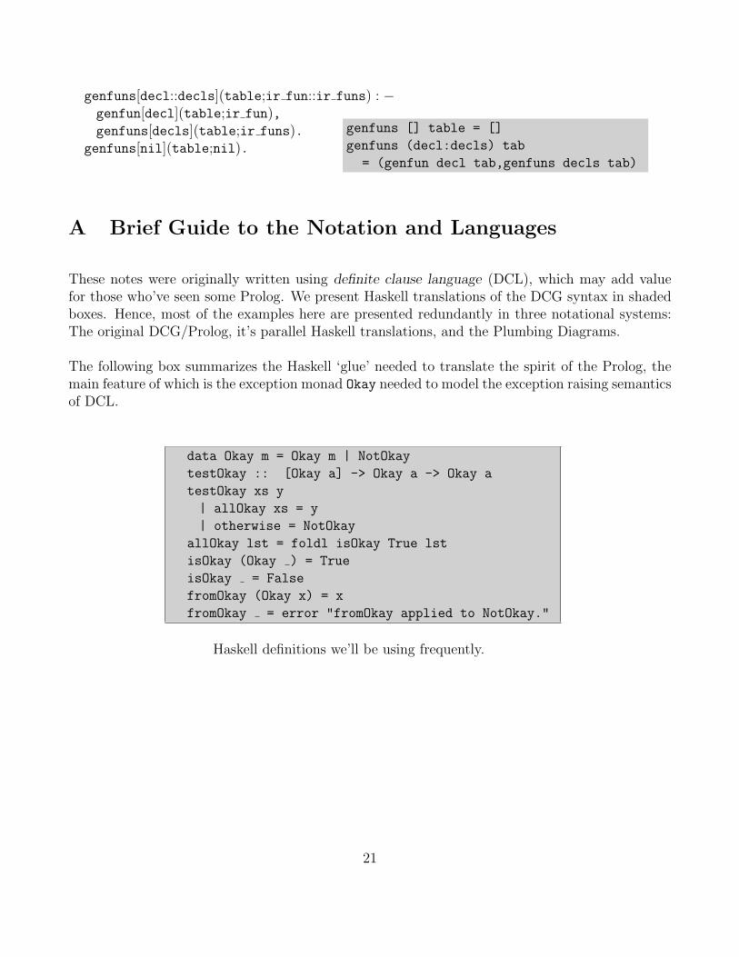
The following box summarizes the Haskell ‘glue’ needed to translate the spirit of the Prolog, themain feature of which is the exception monad Okay needed to model the exception raising semanticsof DCL.

data Okay m = Okay m | NotOkay

testOkay :: [Okay a] -> Okay a -> Okay a

testOkay xs y

| allOkay xs = y

| otherwise = NotOkay

allOkay lst = foldl isOkay True lst

isOkay (Okay ) = True

isOkay = False

fromOkay (Okay x) = x

fromOkay = error "fromOkay applied to NotOkay."

Haskell definitions we’ll be using frequently.

21