Atm Sci 950 Course Syllabus, Page 1

Atm Sci 950 – Seminar on Topics in Atmospheric Sciences:

Numerical Weather Prediction

TR 9:30 – 10:45 am, EMS E170

Fall 2017

Instructor: Prof. Clark Evans

Contact: (414) 229-4469, evans36@uwm.edu, EMS W401

Office Hours: TR 11:00 am – 12:15 pm, by appointment, or stop by anytime.

Prerequisites: Graduate standing, nominally in the atmospheric sciences.

Course Website: http://derecho.math.uwm.edu/classes/AtmSci950.html

Course Overview

Numerical weather prediction can broadly be defined as the application of numerical methods to

solve the primitive equations that describe the atmosphere to obtain a weather forecast. There exist

multiple such methods, however, each with their strengths and weaknesses, and none provide exact

solutions to the primitive equations. Subsidiary to these methods are concepts such as grid

discretization, map projections, numerical stability, and diffusion, each of which can influence the

quality of a given numerical model forecast.

Furthermore, there exist important non-linear physical processes that we cannot explicitly simulate

with a numerical model. To some extent, these physical processes are those associated with what

we typically consider ‘interesting’ weather, particularly clouds and precipitation. Whether due to

their complexity, the spatiotemporal scales on which they operate, and/or our understanding of the

relevant physics and dynamics, we approximate these physical processes within numerical models

in what are known as physical parameterization packages.

Even if there did exist a perfect model, capable of explicitly and accurately resolving all processes

in the atmosphere, perfect forecasts would still be impossible as we do not have perfect knowledge

of the atmospheric state. Further, even if we had a perfect observational network, with observations

available at an infinite number of times and locations, existing means of processing observations

to obtain a gridded numerical representation of the initial atmospheric state are not perfect. Given

the substantial sensitivity of numerical model forecasts to miniscule uncertainty in the atmospheric

state, this poses a stringent upper bound upon the predictability of meteorological phenomena.

One goal of this class is to expose the innards of the ‘black box’ that can be a numerical weather

prediction model. To that end, this class is organized around the three major themes of numerical

methods, physical parameterizations, and data assimilation. Collectively, these themes could serve

as the basis for at least eight semesters’ worth of material: two on numerical model formulation,

five on physical process parameterization, and one on data assimilation. Thus, in designing this

class, depth has necessarily been sacrificed to some extent in favor of breadth. Though this class

may not equip you to become a numerical model developer, the expectation is that you will become

an informed end-user of numerical weather prediction models. Inherent to this is the development

Atm Sci 950 Course Syllabus, Page 2

of your ability to design your own numerical simulation experiments, understand the strengths and

weaknesses of existing numerical weather prediction models, and interpret the output from each.

Learning Objectives

Upon the completion of this course, students will be able to:

Conceptually describe and practically evaluate strengths and weaknesses of the spatial and

temporal differencing, physical process parameterization, and ensemble data assimilation

methods used in modern grid- based numerical weather prediction models.

Configure and execute numerical model simulations to test scientific hypotheses related to

forecast sensitivity to numerical model configuration and/or the physics and dynamics of

meso- to synoptic-scale meteorological phenomena.

Textbook Information

There is one required text for this course: Numerical Weather and Climate Prediction by T. T.

Warner, published by Cambridge Press. We will cover most of the material in Chapters 1-6 in

class, while Chapters 9-11 will prove useful with respect to the course project.

There is one optional text for this course: Parameterization Schemes by D. Stensrud, published

by Cambridge Press. This text is a recommended resource for physical process parameterization,

and the required text makes frequent reference to this text in its Chapters 4 and 5.

I recommend printing a copy of “A Description of the Advanced Research WRF Version 3.” It

places much of what will be covered during the course into the context of a real-world numerical

model, the WRF-ARW model, that you will gain experience in using as part of the course project.

For the data assimilation section of this course, we will make extensive use of the freely-available

Data Assimilation Research Testbed (DART) Lab Exercises and Tutorial. These are excellent

introductions to ensemble data assimilation methods and practical applications.

If you do not have experience using a Linux-/Unix-style terminal computing environment, you

may wish to purchase a text designed to help new users become familiar with such environments.

One recommendation is A Practical Guide to Linux Commands, Editors, and Shell Programming

by Mark G. Sobell. Alternatively, chapters 7 and 8 of the UWM Research Computing User’s Guide

provide a robust yet free resource for introductory Linux/Unix computing.

Finally, if you do not have much computer programing experience, you may wish to complete one

or more tutorials for a language of your choice. For example, many graduate classes in our program

use MATLAB, for which MathWorks provides a set of free introductory tutorials. Python’s

popularity in the atmospheric sciences and beyond has grown exponentially in recent years, and

innumerable free general and atmospheric-science-specific tutorials are available online.

FORTRAN has a long legacy in the atmospheric sciences, and there are many FORTRAN 77 and

FORTRAN 90 tutorials available online. You are free to use any language of your choice, however.

Atm Sci 950 Course Syllabus, Page 3

Grading

Your grade in this course will be based upon the following:

40% Course Project

60% Assignments [Eight in total, each worth 7.5% of your final grade.]

The course project, including relevant deadlines, is described in detail at the end of this syllabus.

The purpose of the project is to allow you to apply many of the foundational concepts underpinning

numerical weather prediction; gain experience in designing and executing scientific experiments,

and gain experience in using the WRF-ARW numerical model in supercomputing environments.

There will be eight assignments given during the semester: one on model compilation, three on

numerical methods, one on physical parameterization, and three on data assimilation. Two of the

numerical methods and all of the data assimilation assignments use toy models to illustrate key

course concepts, while the other numerical methods assignment and the physical parameterization

assignment use full-physics numerical simulations of an observed weather event to illustrate how

assumptions inherent to the chosen simulation method influence forecast quality and variability.

Depending on their length, each assignment is generally due between one and two weeks after the

class in which it is assigned. The tentative date for each assignment to be assigned is provided in

the schedule below. Late work is accepted only in the case of an excused absence.

Finally, your attendance is expected at each regularly-scheduled class meeting. This includes not

using your cell phone, tablet, etc., to snap with your friends or browse the Internet during class!

You are allowed three unexcused absences during the semester without penalty. Your course grade

will be deducted by one sub-grade (e.g., A to A-, A- to B+, etc.) for each successive absence.

Grades will be assigned based on the following scale:

A 92.5-100% A- 90-92.49% B+ 87.5-89.99% B 82.5-87.49%

B- 80-82.49% C+ 77.5-79.99% C 72.5-77.49% C- 70-72.49%

D+ 67.5-69.99% D 62.5-67.49% D- 60-62.49% F 0-59.99%

A grade of an “A” is intended to reflect your mastery of the presented material. Grades of “B” and

“C” are intended to reflect minor and major deficiencies, respectively, in your mastery of the

presented material. Grades of “D” and “F” reflect no mastery of the presented material. Minor

deficiencies include incomplete attribution while major deficiencies include incorrect attribution.

Course Outline

The following outline is provided only as a guideline and is subject to change.

Atm Sci 950 Course Syllabus, Page 4

September 5 Welcome; Project Overview; Computing Environment Introduction

Assignment 1: WRF Compilation (due September 21)

September 7 NWP Overview; Intro to Numerical Methods (Chapter 1, Section 3.1)

September 12 Equations; Resolved vs. Unresolved Scales; Acoustic Waves (Chapter 2)

September 14 Grid Point Methods (Section 3.2.1)

September 19 Vertical Coordinates; Upper Boundary Conditions (Sections 3.4.8, 3.6)

September 21 Finite Difference Methods (Section 3.3)

September 26 Grid Staggering; Truncation Error (Section 3.4.1)

September 28 Linear Stability (Section 3.4.2)

Assignment 2: Differencing Properties and Linear Stability (due Oct 12)

October 3 Numerical Dispersion; Time Difference Properties (Sections 3.4.3, 3.4.4)

October 5 Aliasing; Non-Linear Instability; Diffusion (Sections 3.4.5 to 3.4.7)

Assignment 3: Numerical Dispersion and Diffusion (due October 12)

October 10 Lateral Boundary Conditions (Section 3.5)

October 12 Microphysical Parameterization Overview (Section 4.2)

Assignment 4: WRF Practical – Lateral Boundary Conditions (due Oct 26)

October 17 Microphysical Parameterization Applications

October 19 Convection Parameterization Overview (Section 4.3)

October 24 Convection Parameterization Applications

October 26 PBL Parameterization Overview (Section 4.4)

October 31 PBL Parameterization Applications

Assignment 5: WRF Practical – Physical Parameterizations (due Nov 14)

November 2 Land-Surface Process Parameterization (Chapter 5)

November 7 Radiation Parameterization (Section 4.5)

November 9 Intro to Data Assimilation; Observations; Spin-Up (Sections 6.1 to 6.4)

November 14 Overview of Data Assimilation Principles (Section 6.5)

Assignment 6: Introduction to Data Assimilation (due November 28)

Atm Sci 950 Course Syllabus, Page 5

November 16 Extended and Ensemble Kalman Filters (Sections 6.11.2 and 6.11.3)

November 21 Ensemble Kalman Filter I: Statistical Formulation in 1-D

(DART Lab Section 1; DART Tutorial Section 1)

November 23 NO CLASS – Thanksgiving Holiday

November 28 Ensemble Kalman Filter II: Multivariate and Non-Identity Assimilation

(DART Lab Section 2; DART Tutorial Sections 4 and 5)

Assignment 7: DART Exercises, Part I (due December 7)

November 30 Ensemble Kalman Filter III: Observation Localization

(DART Lab Section 3; DART Tutorial Section 8)

December 5 Ensemble Kalman Filter IV: Other Ensemble Filter Variants

(DART Lab Section 4; DART Tutorial Section 6)

Assignment 8: DART Exercises, Part II (due December 14)

December 7 TBD (Catch-Up, Final Project Q&A, and/or Ensemble Kalman Filter V:

Inflation via DART Tutorial Sections 9 and 12)

December 12 Project Presentations

December 14 Project Presentations; Course Evaluations

I will be on travel for at least one class – October 10 – and possibly also October 12. Although the

schedule above does not indicate this, we will attempt to make up any missed classes with Friday

morning meetings on October 6 and/or 13 (or another mutually-agreed upon date and time).

I expect you to read the chapters and/or sections of the text listed above prior to each class period.

In this way, the material to which you will be exposed in class will be your second, instead of your

first, interaction with the material, increasing the likelihood of information retention.

Course Credit Hour Statement

This course is a three credit course. This means that this class represents an investment of time of

at least 144 hours by the average student. Of these 144 hours, 35 are associated with in-class

instruction and examinations, 35 are associated with the completion of the course project, 40 are

associated with the completion of course exercises, and the remaining 34 are associated with each

student’s study of course materials.

Departmental Regulations

All room changes or course cancellations will be posted on departmental letterhead only.

Atm Sci 950 Course Syllabus, Page 6

University Regulations

University-Wide Rights and Regulations

The University of Wisconsin-Milwaukee has established a series of policies relating to student

rights and regulations in this and all UWM-offered courses. You are encouraged to read through

these policies at http://uwm.edu/secu/syllabus-links/ at your earliest convenience. Please notify me

if you need special accommodations to meet any course requirements.

Statement of Academic Misconduct

The university has a responsibility to promote academic honesty and integrity and to develop

procedures to deal effectively with instances of academic dishonestly. Students are responsible for

the honest completion and representation of their work, for the appropriate citation of sources, and

for respect of others’ academic endeavors. Further information can be found at

http://uwm.edu/academicaffairs/facultystaff/policies/academic-misconduct/.

Statement of Sexual Harassment

Sexual harassment is reprehensible and will not be tolerated by the University. It subverts the

mission of the University and threatens the careers, educational experience, and well-being of

students, faculty and staff. The University will not tolerate behavior between or among members

of the University community which creates an unacceptable working environment. The policy on

discriminatory conduct, including sexual harassment, can be found at

http://www4.uwm.edu/secu/docs/faculty/2847_S_47_Discr_olicy_clean.pdf.

Atm Sci 950 Course Syllabus, Page 7

Course Project: Description, Evaluation, and Helpful Resources

Fall 2017

Description

The purpose of the project is three-fold:

To apply many of the foundational concepts underpinning numerical weather prediction.

To allow you to gain experience with designing and executing scientific experiments.

To allow you to gain experience in using the WRF-ARW numerical model.

Ideally, your course project should involve the study of something related to your thesis research.

However, it cannot represent something that you would otherwise conduct in support of your thesis

research. Your course project can motivate further simulations or analyses that end up comprising

a part of your thesis research but cannot be something that you were otherwise going to do already.

If you are in your first year of study and have limited insight as to your thesis research, I encourage

you to speak with your faculty advisor soon to get a general idea for your thesis research.

There exist two broad forms that your project may take, with potential project ideas listed below

each not necessarily being all-encompassing. Be creative with your project idea. If you’re not sure

if something can be done using a numerical model, please ask – it probably can be in some fashion!

You may conduct multiple simulations of a given meteorological phenomenon or event to

obtain insight regarding its predictability.

o Idea 1: Use different model initial conditions (e.g., from different models or at

different grid spacings from the same model) to quantify sensitivity to the initial

atmospheric state.

o Idea 2: Use initial conditions from a model’s 6-h forecast and from its subsequent

0-h analysis to demonstrate the impact of data assimilation on forecast evolution.

o Idea 3: Use different lateral boundary conditions (e.g., from different models or at

different grid spacings from the same model) to quantify sensitivity to prescribed

lateral boundary information.

o Idea 4: Use different surface data (e.g., different sea surface temperature datasets,

fixed vs. time-varying sea surface temperature data, or different soil moisture and

temperature datasets) to quantify sensitivity to atmospheric-surface interaction.

You may conduct multiple simulations of a given meteorological phenomenon or event to

quantify the sensitivity in the numerical simulation of that phenomenon to variation in an

appropriately-chosen model configuration selection.

Atm Sci 950 Course Syllabus, Page 8

o Idea 1: Use different selections for a single class of physical parameterization, or

whether or not a specialized type of parameterization (e.g., urbanization, ocean/lake

model, or shallow convection) is used.

o Idea 2: Use different selections for parameters inherent to a single parameterization

(e.g., parameters controlling vertical mixing in the planetary boundary layer or how

soil moisture is updated in response to rainfall).

o Idea 3: Within reason for the phenomenon being studied, vary the horizontal and/or

vertical grid characteristics (e.g., grid spacing, grid size or placement, number or

distribution of vertical levels, or the choice of vertical coordinate).

o Idea 4: Use different selections for selected parameters influencing model dynamics

(e.g., vertical velocity damping, explicit numerical diffusion, nudging, diffusion

coefficients, time stepping method, or the finite differencing formulation).

Each of you will likely conduct what are known as “real-data” numerical simulations, or those of

an actually-observed phenomenon or event, that are initialized with a model-derived synthesis of

observations. The WRF-ARW numerical model is ideally suited for such studies and, as such, is

the model that you will gain experience with using for your project.

Robust numerical simulations require an appropriate experimental design, motivated by physical

understanding and previous research, that lends itself to a testable hypothesis; model configuration,

to facilitate the implementation of the experimental design; and physical analysis, designed to test

the hypothesis underpinning the numerical simulation experiment(s). Helpful resources for each

of these elements are provided below. Note that the experimental design should be appropriate to

a course of a semester in length but also to a graduate student’s level of understanding; i.e., more

robust than a capstone project but not as robust as a thesis or dissertation.

There exist two deliverables from your class project:

A presentation of no more than 15 minutes in length, to be given at the end of the semester

to an audience of your classmates.

A typed report of no more than 10 double-spaced pages, due at the time of the presentation.

Note that the abstract, figures, tables, and references do not count against the page limit.

The presentation should be given in the format of that given at American Meteorological Society

and American Geophysical Union conferences. Typically, this involves ~12 minutes for your

presentation and ~3 minutes for questions from the audience. The presentation should detail what

you are studying, the hypothesis being tested in your study, the experimental design used to test

that hypothesis, and the results of your study. Where possible, you should also describe possible

directions for future research. Each slide should be clearly explained and legible from the back of

the room. Note that a good estimate is one slide per minute. Large tables are not recommended.

Atm Sci 950 Course Syllabus, Page 9

Figures are preferable to text, though there exist instances where several bullet points’ worth of

text on a slide are unavoidable. I recommend that you practice your presentation more than once

prior to giving it in class. Recorded presentations given at previous meetings are a great way to get

ideas as to how to (or how not to) organize your presentation.

The report should be in the format of that used by American Meteorological Society and American

Geophysical Union publications. Information regarding manuscript formatting and references is

available from the American Meteorological Society. There is no limit on the number of figures

or tables that you include within your report within reason. As with the presentation, the report

should clearly describe what you are studying, the hypothesis being tested in your study, the

experimental design used to test that hypothesis, and the results of your study. Where possible,

you should also describe possible directions for future research.

A suggested course project calendar is provided at the end of this document. Further, to ensure that

you will have sufficient time to complete the project, I have established the following milestones:

Project Idea: Thursday, September 28

Experimental Design: Thursday, October 19

As needed, you should meet with me to discuss potential project ideas and/or so that I can help

point you to previous studies (where applicable) that can help you shape your specific project idea.

Please contact me as soon as possible to schedule a time for this meeting if you are so inclined.

To help you formulate your experimental design, you are required to meet with me prior to the

deadline for the experimental design to be finalized. You should come prepared with a draft outline

of your experimental design, including a draft (yet complete) WRF namelist.input to be used for

your numerical simulation(s). Be prepared to discuss the hypothesis to be tested by your project,

the anticipated model configuration and justification thereof, and the intended analysis method(s)

to be used to analyze simulation output. We will discuss and refine each of these elements during

our meeting. Please contact me to schedule this meeting as soon as you are ready.

I am happy to meet with you on an as-needed basis to discuss progress made and challenges faced

as you work toward the completion of your project. There are many challenges that you will likely

encounter, include the model crashing, results that are not consistent with your hypothesis, and

difficulty in post-processing, visualizing, and/or analyzing model output. While you should always

attempt to address these challenges yourself first before seeking guidance, I am here to help.

Evaluation

Your grade on the course project will be determined considering the following elements:

Experimental Design (35%): Was the student well-prepared for the experimental design

meeting? Are the chosen experimental design and model configuration appropriate for the

study of the meteorological phenomenon and/or event being studied? Are relevant

Atm Sci 950 Course Syllabus, Page 10

references cited and briefly discussed to provide evidence supporting the experimental

design and motivation for the research? Is sufficient information conveyed, particularly in

the project report, such that the results could be independently reproduced?

Simulation Verification (10%): Is simulation verification performed? Are appropriate

simulation verification methods employed? Are departures from reality documented, and

theories as to why such departures exist (where appropriate) well-posed?

Simulation Interpretation (35%): Is appropriate physical and dynamical insight provided

to interpret the output from the numerical simulation(s) conducted? Are appropriate

connections made, where possible, between the results from the study and those provided

by previous published research?

Presentation and Report Quality (10%): Are the presentation and report well-written?

Do they adhere to the guidelines for each outlined above? Are all figures clear, legible,

relevant, and adequately explained? Were questions from the audience handled well at the

end of the presentation?

Peer Evaluation (10%): A Google Docs-based survey will be used to anonymously collect

student feedback from each student’s presentation. One survey question will ask you to

identify the key message from each presentation. This will be used to assess how well you

conveyed your findings to the audience. Remaining questions will be used to provide you

with constructive feedback on your project and presentation.

This breakdown forms the basis for the project grading rubric, a copy of which is provided at the

end of this document.

Please note that the experimental design and simulation interpretation are given substantially

greater weight than the remaining project elements. While simulation verification and quality of

presentation are important, most important is whether your project design and results from the

project well-posed. Of particular importance with respect to simulation interpretation is that you

go beyond describing the results of your simulation(s) to describe the why and how behind your

results; e.g., not just that differences exist between simulations, but why do they exist?

Helpful Resources

Many of you likely enter this class with little experience in a Linux computing environment, with

designing your own scientific experiments, and with numerical weather prediction in general.

Thus, the concept of a course project in which you will be utilizing a Linux computing environment

to design and execute your own numerical simulations may seem daunting at first. Fortunately,

there exist many resources that can guide you through the process, described below.

The first resource, and perhaps the most direct, is your instructor. While I cannot and will not

complete the project for you, I am happy to help address questions. Please do not hesitate to ask –

Atm Sci 950 Course Syllabus, Page 11

in office hours, before or after class, via e-mail, or simply by stopping into my office if the door is

open. With this comes the expectation, however, that you will not wait until right before something

is due to ask questions, nor that you will ask questions without having attempted to find the answer

on your own first. Allow yourself plenty of time for each stage of the project so that you can have

any questions addressed, recognizing that rarely does anything work right the first time when you

are conducting numerical simulations!

Using a Linux Environment: The supercomputer on which you will be configuring, conducting,

and analyzing the output from your numerical simulations uses a flavor of Linux as its operating

system. Consequently, you will want to become familiar with at least basic commands on the Linux

command line. There exist a number of web-based resources that can help you to do so; simply

conduct a web search for “common Linux commands.” You may also wish to rent or purchase a

book; one such book that comes highly recommended is A Practical Guide to Linux Commands,

Editors, and Shell Programming by Mark G. Sobell. As of this writing, it can be rented from

Amazon for ~$14 or purchased new for ~$25.

If you’d prefer something cheaper (free), UWM’s Research Computing Support has put together

a general guide to research computing. Chapters 7 and 8 of this document introduce the Unix/Linux

command line and to shell scripting, respectively. It may be accessed from:

http://www.peregrine.hpc.uwm.edu/Webdocs/research-computing.pdf

Experimental Design Basics: When you meet with me to discuss your project idea, we will refine

your ideas for the experimental design. However, it would behoove you to become familiar with

basic tenets of experimental design prior to us doing so. Chapter 10 of the course text (Numerical

Weather and Climate Prediction) provides extensive information regarding how to appropriately

design a numerical simulation. The following article from the Bulletin of the American

Meteorological Society, by the author of our course text, provides similar information:

Warner, T. T., 2011: Quality assurance in atmospheric modeling. Bull. Amer. Meteor. Soc., 92,

1601–1610. (doi: http://dx.doi.org/10.1175/BAMS-D-11-00054.1)

A presentation from 2012 by Chris Davis of the National Center for Atmospheric Research

provides a condensed form of the information from this article, particularly in the context of

designing a numerical experiment using the WRF-ARW model. It can be accessed at:

http://www2.mmm.ucar.edu/wrf/users/workshops/WS2012/ppts/discussion1.pdf

Getting Started with WRF: There exist many references that can assist you in compiling,

configuring, and executing the WRF-ARW model. The first that you should work through is the

WRF Online Tutorial, available from the National Center for Atmospheric Research at:

http://www2.mmm.ucar.edu/wrf/OnLineTutorial/index.htm

Atm Sci 950 Course Syllabus, Page 12

This tutorial will guide you through the process of obtaining model code, compiling the model,

setting up the model for a well-tested trial simulation, and running the model itself. Note that not

all portions of the tutorial will be applicable for our applications, nor have they all been updated

for the most recent model releases. The first assignment will provide further details specific to our

chosen supercomputing environment and the current WRF-ARW model release.

As you work through the tutorial, as well as after completing the tutorial, you may also find the

following resources helpful:

WRF-ARW User’s Guide: Describes the WRF-ARW model and available configuration

options – but not necessarily why a given option would be selected – in detail. You should

refer to the User’s Guide for model version 3.9.

WRF Tutorial Presentations: An excellent source of additional reference information

regarding WRF-ARW configuration, execution, and interpretation of model output.

WRF Physics References: This page provides full citation information for all available

user-selectable model configuration options available within the WRF-ARW model. If

your project involves examining the sensitivity of a numerical simulation to the choice of

physical parameterization, these references will help you better understand how each is

formulated as it appears in WRF-ARW. You may also refer to other published works, such

as the Parameterization Schemes text by David Stensrud, for this information.

When you reach the point of conducting your own numerical simulations, you will need to provide

data to serve as initial and lateral boundary conditions for these simulations. These are typically

provided by another numerical model or by a model-derived reanalysis product, though they need

not be limited to such. At a minimum, they will provide data for the initial and future atmospheric,

land-surface, and water-surface state.

Unless we jointly decide that an alternative course of action is appropriate, I recommend that you

utilize widely-available and well-tested data sets for your initial and lateral boundary conditions.

These data can be obtained from the University Corporation for Atmospheric Research’s Research

Data Archive at http://rda.ucar.edu/. For retrospective simulations of a given meteorological

phenomenon, I recommend that you utilize reanalysis data for initial and lateral boundary

conditions. There exist several such datasets available in the Research Data Archive, and I

generally recommend the ERA-Interim dataset in GRIB format for most applications.

For retrospective conditions of the predictability of a given meteorological phenomenon, I

recommend that you utilize numerical model analysis and forecast data for initial and lateral

boundary conditions. These can be obtained from the Research Data Archive in the Unidata

Historical IDD Archive, also in GRIB format. Note that these data will likely need to be processed

somewhat for use with WRF-ARW. If you are not sure what data to obtain or whether processing

of the data is needed, please ask.

Atm Sci 950 Course Syllabus, Page 13

WRF “Best Practices”: As a community model that has been in existence for over ten years, there

have been many studies conducted utilizing the WRF-ARW model. Consequently, there exists a

wide body of literature documenting the performance of many model configuration selections in

simulations of a wide range of atmospheric phenomena.

Best practices for configuring and using the WRF-ARW model are available from the National

Center for Atmospheric Research in the following documents:

General Best Practices:

http://www2.mmm.ucar.edu/wrf/users/workshops/WS2014/ppts/best_prac_wrf.pdf

General Best Practices:

http://www2.mmm.ucar.edu/wrf/users/tutorial/201707/best_prac.pdf

WRF Dynamics Best Practices: See the first set of presentations at

http://www2.mmm.ucar.edu/wrf/users/workshops/WS2015/WorkshopPapers.php

Sample Namelists for Specific Applications:

http://www2.mmm.ucar.edu/wrf/users/docs/user_guide_V3/users_guide_chap5.htm#examples

Experimental Design and Literature Review: You should review the published literature –

particularly from journals published by the American Meteorological Society, American

Geophysical Union, and U.K. Royal Meteorological Society – prior to finalizing your experimental

design. For instance, you may wish to search for manuscripts that report on numerical modeling

studies conducted to study the meteorological phenomenon that you wish to study. Typically, such

studies will provide justification as to the specific model configuration selections made.

Alternatively, particularly if you wish to examine the sensitivity to a specific model configuration

selection in numerical simulations of a given meteorological phenomenon, you may wish to search

for manuscripts that report on the results of similar studies for other phenomena. Typically, such

studies will provide information as to why a given selection performs as it did for that case(s)

studied. The same journals as described above should also be consulted when taking this approach.

Note that you may have to use the UWM Library’s “Search@UW” feature or be connected to the

campus network to access some articles, particularly from 2015-onward. You will not be able to

directly access “Early Online Release” papers from the AMS. Please let me know if you need

assistance in accessing a specific article and I will be happy to help.

I also anticipate that you will apply insight regarding model configuration and simulation design

that we cover in class to your experimental design. For example, prior to the experimental design

being finalized, we will address in lecture considerations related to model spin-up, horizontal grid

spacing, the choice of model time step, map projections, domain extent as a function of the

placement of the simulation domain’s lateral boundaries, and vertical grid spacing.

Atm Sci 950 Course Syllabus, Page 14

Post-Processing: Once a numerical simulation is complete, your next task is to interpret its output.

In most cases, this involves post-processing the model output into a format that a given analysis

or display package can natively read in. Some packages (e.g., NCL, wrf-python) handle this on-

the-fly, whereas others (e.g., GrADS, RIP) require the user to first run another program. Post-

processing often aids in computing derived fields from raw model output and in destaggering the

model output from its computational grid to a more user-friendly uniform grid, though it requires

extra computational time and disk space.

The WRF Online Tutorial, WRF Tutorial Presentations, and WRF-ARW User’s Guide (primarily

Chapter 9) provide information about WRF-ARW simulation post-processing and visualization.

Specific information about using NCL to visualize WRF-ARW model data is available from both

the WRF Online Tutorial and the NCL webpage. Information about using wrf-python to visualize

WRF-ARW model data is available from the wrf-python webpage. Information about using

ARWpost or UPP to process data for display in GrADS, or RIP, is available from the WRF-ARW

User’s website. Other programs that can read in netCDF data (e.g., MATLAB, IDL, IDV, ncview)

can visualize WRF-ARW data, but often on the native model grid and without the diagnostic

computations other tools provide.

General techniques that you may wish to employ to analyze model output are outlined in Chapter

11 of the course text. We will discuss the types of analysis that you wish to conduct at the time

when we meet to discuss your experimental design.

Forecast Verification: An often overlooked, but vitally important, component of a numerical

simulation experiment is forecast verification. In other words, how accurate was the forecast? This

typically involves comparing the simulation output to available observations, of which there are

many types in many different formats. As a part of our discussion of your project design, we will

discuss appropriate means of forecast verification, including the data best suited to assessing

forecast quality and where to obtain such data.

There exist many methods by which forecast quality may be assessed, each of which have their

own strengths and limitations. The Centre for Australian Weather and Climate Research’s

webpage on forecast verification is a highly recommended resource with respect to both general

and specific considerations for forecast verification. It is available at:

http://www.cawcr.gov.au/projects/verification/

You may also wish to review Chapter 9 of the course text. Studies in the published literature also

often involve some form of forecast verification, and considering what others have done before is

a good way to develop ideas as to how you should assess forecast quality.

Atm Sci 950 Course Syllabus, Page 15

Suggested Course Project Calendar

The calendar below is provided as a guide for you to follow as you work toward completing the

course project. You may choose or be able to work through the project at a slower or faster pace

than is depicted below. You may also choose to utilize different resources when formulating your

project idea or experimental design. These are perfectly acceptable alternatives.

The below outline assumes that the first week’s technological activities will provide you with

sufficient Linux terminal experience to be prepared for the rest of the course project. If you need

assistance with this or anything throughout the semester, please let me know.

Week Of Technological Activities Other Activities

September 4 Configure and compile WRF-ARW. Brainstorm general project

ideas. Meet with your advisor

if/as needed when doing so.

September 11 Complete the January 2000 test case in

the WRF Online Tutorial.

Review Chapter 10 of the

course text, Warner (2011), and

Chris Davis’ 2012 presentation.

September 18 Post-process and visualize output from

the January 2000 test case, following

the WRF Online Tutorial.

Meet with Prof. Evans to

formalize and refine your

project idea.

September 25 Review WRF Tutorial Presentations. Begin literature review in

support of developing your

experimental design.

October 2 Continue to review WRF Tutorial

Presentations. Emphasize identifying

general best practices. Begin drafting

your experimental design.

Continue literature review.

Emphasize identifying specific

model configuration selections

relevant to your project idea.

October 9 Refine your draft experimental design. Complete literature review.

Meet with Prof. Evans to

formalize experimental design.

October 16 Obtain initial and lateral boundary

condition data for your simulation(s).

Complete geogrid.exe, ungrib.exe, and

metgrid.exe for your first simulation.

Begin writing project report.

Focus upon your scientific

motivation and summarizing

your literature review.

Atm Sci 950 Course Syllabus, Page 16

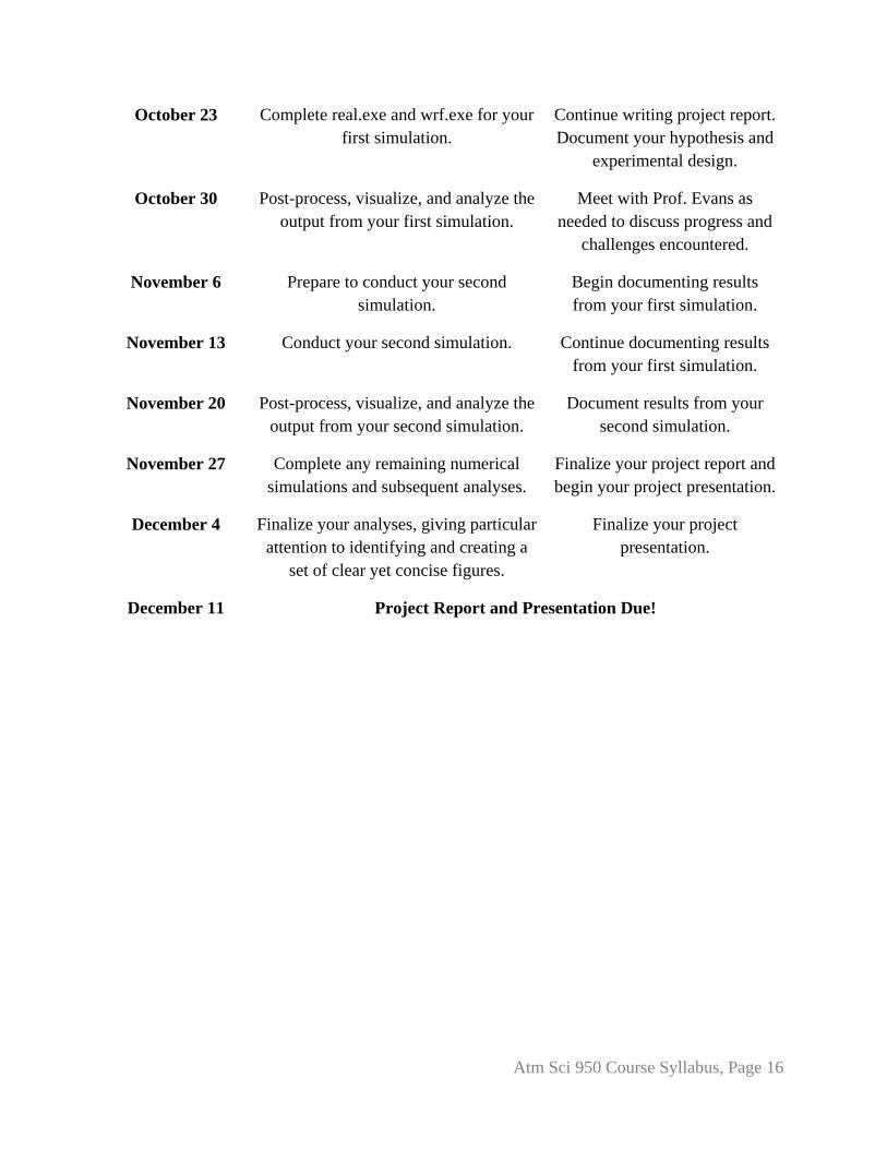
October 23 Complete real.exe and wrf.exe for your

first simulation.

Continue writing project report.

Document your hypothesis and

experimental design.

October 30 Post-process, visualize, and analyze the

output from your first simulation.

Meet with Prof. Evans as

needed to discuss progress and

challenges encountered.

November 6 Prepare to conduct your second

simulation.

Begin documenting results

from your first simulation.

November 13 Conduct your second simulation. Continue documenting results

from your first simulation.

November 20 Post-process, visualize, and analyze the

output from your second simulation.

Document results from your

second simulation.

November 27 Complete any remaining numerical

simulations and subsequent analyses.

Finalize your project report and

begin your project presentation.

December 4 Finalize your analyses, giving particular

attention to identifying and creating a

set of clear yet concise figures.

Finalize your project

presentation.

December 11 Project Report and Presentation Due!

Atm Sci 950 Course Syllabus, Page 17

Name: ____________________________

NWP Course Project: Instructor Evaluation

Experimental Design (35%)

Were all deadlines for the project idea and experimental design met? Was the student well-

prepared for the experimental design meeting?

Are the chosen experimental design and model configuration appropriate for the study?

Are relevant references cited to demonstrate the appropriateness of the experimental design

and provide motivation for the research, proposed and/or conducted?

Is sufficient information provided to ensure the reproducibility of the results?

Simulation Verification (10%)

Is simulation verification performed? Are appropriate verification methods used to do so?

Are departures from reality documented, and theories as to why such departures exist

(where appropriate) well-posed?

Atm Sci 950 Course Syllabus, Page 18

Simulation Interpretation (35%)

Is appropriate insight provided to interpret simulation output? What are the key results?

Are appropriate connections made where possible between the results and previous works?

Presentation and Report Quality (10%)

Are the presentation and report well put-together (presented and written)?

Did the presentation and report adhere to the timing and length guidelines?

Are all figures clear, legible, relevant, and adequately explained?

Were audience questions handled well?

Peer Evaluation (10%)

How well was the key message of the presentation interpreted by the students?

Anonymously summarize peer feedback: