5. Assessment of the Deepwater Flatfish Stock Complex in the Gulf of Alaska

By Carey R. McGilliard1 and Wayne Palsson2

1Resource Ecology and Fisheries Management Division 2Resource Assessment and Conservation Engineering Division

Alaska Fisheries Science Center National Marine Fisheries Service

National Oceanic and Atmospheric Administration 7600 Sand Point Way NE., Seattle, WA 98115-6349

Executive Summary

Summary of Changes in Assessment Inputs (1) 2014-2015 catch data were included in the model (2) 2013 catch was updated to include October-December catch in that year (3) 2014 and 2015 fishery length composition data were added to the model and 2013 fishery length

composition data were updated to include October-December data in that year (4) The 2015 survey biomass index was added to the model (5) Survey length composition data for 2015 were added to the model (6) 2015 Survey ages measured within each length bin were added to the model (7) Effective sample sizes for fishery and survey length and age data were changed to the number of hauls

for which length or age data were measured, respectively. (8) Length and age composition data were iteratively re-weighted using the harmonic mean of effective

sample size, with effective sample size calculated according to the methods described in McAllister and Ianelli (1997).

(9) Bias adjustment parameters were updated (10) Length-based fishery selectivity was estimated using an asymptotic selectivity curve (double normal

selectivity without descending limbs). In the previous model, dome-shaped selectivity was estimated, but standard deviations associated with descending limb parameter estimates were very large, indicating that data are not informative about the descending limb parameter.

Summary of Results The key results for the assessment of the deepwater flatfish complex are compared to the key results from accepted 2014 assessment in the table below. The results for Dover sole are based on the author’s base case model and Tier 3a management.

Species Quantity

As estimated or As estimated or specified last year for: recommended this year for:

2015 2016 2016* 2017*

Dover sole

M (natural mortality rate) 0.085 0.085 0.085 0.085 Tier 3a 3a 3a 3a Projected total (3+) biomass (t) 182,160 181,691 141,824 143,007 Projected Female spawning biomass (t) 67,156 67,868 49,179 49,271 B100% 70,544 70,544 56,729 56,729 B40% 28,218 28,218 22,692 22,692 B35% 24,690 24,690 19,855 19,855 FOFL 0.12 0.12 0.12 0.12 maxFABC 0.1 0.1 0.1 0.1 FABC 0.1 0.1 0.1 0.1 OFL (t) 15,749 15,559 10,858 10,924 maxABC (t) 13,151 12,994 9,043 9,097 ABC (t) 13,151 12,994 9,043 9,097

Greenland turbot

Tier 6 6 6 6 OFL (t) 238 238 238 238 maxABC (t) 179 179 179 179 ABC (t) 179 179 179 179

Deepsea sole

Tier 6 6 6 6 OFL (t) 6 6 6 6 maxABC (t) 4 4 4 4 ABC (t) 4 4 4 4

Deepwater Flatfish

Complex

OFL (t) 15,993 15,803 11,102 11,168 maxABC (t) 13,334 13,177 9,226 9,280 ABC (t) 13,334 13,177 9,226 9,280

Status As determined in 2014

for: As determined in 2015 for:

2013 2014 2014 2015 Overfishing no n/a no n/a Overfished n/a no n/a no Approaching overfished n/a no n/a no

*Projections are based on estimated catches of 256.8 t and 345.6 t used in place of maximum permissible ABC for 2015 and 2016, respectively. The 2015 projected catch was calculated as the current catch as of October 10, 2015 added to the average October 10 – December 31 catches over the 5 previous years. The 2016 projected catch was calculated as the average catch from 2010-2014. The maximum permissible ABC for 2017 was used as the projected catch for 2017.

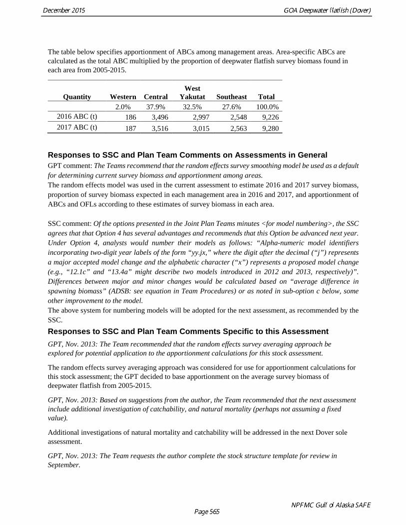
The table below specifies apportionment of ABCs among management areas. Area-specific ABCs are calculated as the total ABC multiplied by the proportion of deepwater flatfish survey biomass found in each area from 2005-2015.

Quantity Western Central West

Yakutat Southeast Total 2.0% 37.9% 32.5% 27.6% 100.0%

2016 ABC (t) 186 3,496 2,997 2,548 9,226 2017 ABC (t) 187 3,516 3,015 2,563 9,280

Responses to SSC and Plan Team Comments on Assessments in General GPT comment: The Teams recommend that the random effects survey smoothing model be used as a default for determining current survey biomass and apportionment among areas. The random effects model was used in the current assessment to estimate 2016 and 2017 survey biomass, proportion of survey biomass expected in each management area in 2016 and 2017, and apportionment of ABCs and OFLs according to these estimates of survey biomass in each area. SSC comment: Of the options presented in the Joint Plan Teams minutes <for model numbering>, the SSC agrees that that Option 4 has several advantages and recommends that this Option be advanced next year. Under Option 4, analysts would number their models as follows: “Alpha-numeric model identifiers incorporating two-digit year labels of the form “yy.jx,” where the digit after the decimal (“j”) represents a major accepted model change and the alphabetic character (“x”) represents a proposed model change (e.g., “12.1c” and “13.4a” might describe two models introduced in 2012 and 2013, respectively)”. Differences between major and minor changes would be calculated based on “average difference in spawning biomass” (ADSB: see equation in Team Procedures) or as noted in sub-option c below, some other improvement to the model. The above system for numbering models will be adopted for the next assessment, as recommended by the SSC. Responses to SSC and Plan Team Comments Specific to this Assessment GPT, Nov. 2013: The Team recommended that the random effects survey averaging approach be explored for potential application to the apportionment calculations for this stock assessment.

The random effects survey averaging approach was considered for use for apportionment calculations for this stock assessment; the GPT decided to base apportionment on the average survey biomass of deepwater flatfish from 2005-2015.

GPT, Nov. 2013: Based on suggestions from the author, the Team recommended that the next assessment include additional investigation of catchability, and natural mortality (perhaps not assuming a fixed value).

Additional investigations of natural mortality and catchability will be addressed in the next Dover sole assessment.

GPT, Nov. 2013: The Team requests the author complete the stock structure template for review in September.

A stock structure template will be completed in 2016.

GPT, Nov. 2013: The Team also recommended that the items listed for future research by the author be pursued.

The 2015 assessment re-visited effective sample sizes, setting effective sample sizes to the number of hauls. The 2015 assessment also re-visited data weighting, as well as the shape of the fishery selectivity curve.

SSC, Dec. 2013: The SSC looks forward to completion of the stock structure template for this complex next year as well as additional investigation of catchability and natural mortality in the next assessment of Dover sole.

A stock structure template will be completed in 2016.

Introduction The "flatfish" species complex previous to 1990 was managed as a unit in the Gulf of Alaska (GOA). It included the major flatfish species inhabiting the region, with the exception of Pacific halibut. The North Pacific Fishery Management Council divided the flatfish assemblage into four categories for management in 1990; "shallow flatfish" and "deep flatfish", flathead sole and arrowtooth flounder. This classification was made because of significant differences in halibut bycatch rates in directed fisheries targeting the shallow-water and deepwater flatfish species. Arrowtooth flounder, because of high abundance and low commercial value, was separated from the group and managed under a separate acceptable biological catch (ABC). Flathead sole were likewise assigned a separate ABC since their distribution over depths overlaps with that of the shallow-water and deepwater groups. In 1993, rex sole was split out of the deepwater management category because of concerns regarding the bycatch of Pacific ocean perch in the rex sole target fishery.

The deepwater complex, the subject of this chapter, is composed of three species: Dover sole (Microstomus pacificus), Greenland turbot (Reinhardtius hippoglossoides) and deepsea sole (Embassichthys bathybius). Dover sole dominates the biomass of the deepwater complex in research trawl surveys and fishery catch (typically over 98%). Little biological information exists for Greenland turbot or deepsea sole in the GOA. More information exists for Dover sole, which allowed the construction of an age-structured assessment model in 2003 (Turnock et al., 2003).

Greenland turbot have a circumpolar distribution and occur in both the Atlantic and Pacific Oceans. In the eastern Pacific, Greenland turbot are found from the Chukchi Sea through the Eastern Bering Sea and Aleutian Islands, in the GOA and south to northern Baja California. Greenland turbot are typically distributed from 200-1600 m in water temperatures from 1-4 °C, but have been taken at depths up to 2200 m.

Dover sole occur from Northern Baja California to the Bering Sea and the western Aleutian Islands; they exhibit a widespread distribution throughout the GOA (Hart, 1973; Miller & Lea, 1972). Adults are demersal and are mostly found at depths from 300 m to 1500 m.

Dover sole are batch spawners; spawning in the GOA has been observed from January through August, peaking in May (Hirschberger & Smith, 1983). The average 1 kg female may spawn 83,000 advanced yolked oocytes in about 9 batches (Hunter, Macewicz, Lo, & Kimbrell, 1992). Although the duration of the incubation period is unknown, eggs have been collected in plankton nets east of Kodiak Island in the summer (Kendall & Dunn, 1985). Larvae are large and have an extended pelagic phase that averages

about 21 months (Markle, Harris, & Toole, 1992). They have been collected in bongo nets only in summer over mid-shelf and slope areas in the GOA. The age or size at metamorphosis is unknown, but pelagic postlarvae as large as 48 mm have been reported and juveniles may still be pelagic at 10 cm (Hart, 1973). Juveniles less than 25 cm are rarely caught with the adult population in bottom trawl surveys (Martin & Clausen, 1995).

Dover sole move to deeper water as they age and older females may have seasonal migrations from deep water on the outer continental shelf and upper slope where spawning occurs to shallower water mid-shelf in summer time to feed (tagging data from California to British Columbia; Demory et al., 1984, Westrheim et al., 1992). Older male Dover sole may also migrate seasonally but to a lesser extent than females. The maximum observed age for Dover sole in the GOA is 59 years.

Fishery Since passage of the MSFMCA in 1977, the flatfish fishery in the GOA has undergone substantial changes. Until 1981, annual harvests of flatfish were around 15,000 t, taken primarily as bycatch by foreign vessels targeting other species. Foreign fishing ceased in 1986 and joint venture fishing began to account for the majority of the catch. In 1987, the GOA-wide flatfish catch increased nearly four-fold, with joint venture fisheries accounting for all of the increase. Since 1988, only domestic fishing fleets are allowed to harvest flatfish. As foreign fishing ended, catches decreased to a low of 2,441 t in 1986. Catches subsequently increased under the joint venture and then domestic fleets to a high of 43,107 t in 1996. Catches then declined to 23,237 t in 1998 and were 22,700 t in 2004.

The GOA deepwater flatfish complex of species is caught in a directed fishery primarily using bottom trawls. Fewer than 20 shore-based catcher-type vessels participate in this fishery, together with about 6 catcher-processor vessels. Fishing seasons are driven by seasonal halibut PSC apportionments, with fishing occurring primarily in April and May because of higher catch rates and better prices. The deepwater flatfish complex catch is dominated by Dover sole (over 98%, typically;Table 1). Dover sole have been taken primarily in the Central GOA in recent years, as well on the continental slope off Yakutat Bay in the eastern GOA (based on fishery observer data).

Deepwater flatfish are also caught in pursuit of other bottom-dwelling species as bycatch. They are taken as bycatch in Pacific cod, bottom pollock and other flatfish fisheries. The gross discard rates for deepwater flatfish across all fisheries are relatively high, with 39% discarded in 2010 and 49% in 2011 (Stockhausen et al., 2011).

Historically, catch of Dover sole increased dramatically from a low of 23 t in 1986 to a high of almost 10,000 t in 1991 (Table 1, Figure 1). Following that maximum, annual catch has declined rather steadily. Catch of Greenland turbot has been sporadic and has been over than 100 t only 5 times since 1978. The highest catch of Greenland turbot (3,012 t) occurred in 1992, coinciding with the second highest catch of Dover sole (8,364 t) since 1978. This was followed by a catch of 16 t for Greenland turbot the next year. Annual catch has been less than 25 t since 1995. Deepsea sole is the least caught of the three deepwater flatfish species. It has been taken only intermittently, with less than a ton of annual catch occurring 14 times since 1978. The highest annual catch occurred in 1998 (38 t), but since then annual catch has been less than 3 t in every year, except for 2009 when 6 t were caught.

Annual catches of deepwater flatfish have been well below the TACs in recent years (Table 2). Annual TACs, in turn, have been set equal to their associated ABCs (Table 2). Low catches relative to the TAC in the deepwater flatfish complex are driven by targeting decisions based on restrictions on halibut PSC. Closures of the deepwater flatfish fishery in 2015 are shown in Table 3. Currently, ABCs for the entire

complex are based on summing ABCs for the individual species. Tier 6 calculations are used to obtain species-specific contributions to the complex-level ABC and OFL for each year because population biomass estimates based on research trawl surveys for Greenland turbot and deepsea sole are considered unreliable and there is little basic biological information from these two species. As such, ABCs for Greenland turbot and deepsea sole are based on average historic catch levels and do not vary from year to year. Since 2003, the ABC for Dover sole has been based on an age-structured assessment model (Turnock et al., 2003).

Data The following table specifies the source, type, and years of all data included in the assessment models.

Source Type Years Fishery Catch biomass 1978-2015 Fishery Catch length composition 1991-2004, 2009-2012 (2005-2008, 2013 data

are excluded), 2014-2015 GOA survey bottom trawl

Survey biomass Triennial: 1984-1999, Biennial: 2001-2015

GOA survey bottom trawl

Catch length composition Triennial: 1990-1999, Biennial: 2003-2015 (1984, 1987, and 2001 data are excluded)

GOA survey bottom trawl

Catch age composition, conditioned on length

Triennial: 1990-1999, Biennial: 2003-2015 (1984, 1987, and 2001 data are excluded)

Fishery The assessment included catch data from 1978 to October 10, 2015 (Table 1, column 3, Figure 1). Fishery length composition data were included in 2cm bins from 6-70cm in 1991-2004 and 2009-2012; data were omitted due to low sample size in 2005-2008 and 2013. Fishery length composition data were voluminous and can be accessed at (http://www.afsc.noaa.gov/REFM/Docs/2015/GOA_Dover_Composition_Data_And_SampleSize_2015.xlsx).

Survey Biomass and Numerical Abundance

Survey biomass estimates originate from a cooperative bottom trawl survey between the U.S. and Japan in 1984 and 1987 and a U.S. bottom trawl survey conducted by the Alaska Fisheries Science Center Resource Assessment and Conservation Engineering (RACE) division thereafter. Calculations for final survey biomass and variance estimates by strata are fully described in Wakabayashi et al. (1985). Survey depth and area coverage was variable over time; the 1990, 1993, and 1996 surveys sampled only 0-500m depths, while the 2001 survey excluded the West Yakutat and Southeast management areas (the eastern GOA). In addition, the 700-1000 m depth range was sampled only in select survey years and areas (Table 4). Maps of survey catch-per-unit-effort (CPUE) for 2011-2015 survey are shown in Figure 2. A random effects model developed for survey averaging (presented at the September 2013 Plan Team Meeting, http://www.afsc.noaa.gov/REFM/stocks/Plan_Team/2013/Sept/SAWG_2013_draft.pdf) was used to estimate survey biomass and variance in missing depth and area strata (Table 4, Table 5). Table 5 describes the random effects model configurations and data used to estimate survey biomass and variance for each missing strata-year combination. The final survey biomass estimates and CVs used in the assessment are shown in Table 6.

Survey size and age composition

Sex-specific survey length composition data and age frequencies of fish by length (conditional age-at-length) were used in the assessment and can be found at (http://www.afsc.noaa.gov/REFM/Docs/2015/GOA_Dover_Composition_Data_And_SampleSize_2015.xlsx). There are several advantages to using conditional age-at-length data. The approach preserves information on the relationship between length and age and provides information on variability in length-at-age such that growth parameters and variability in growth can be estimated within the model. In addition, the approach resolves the issue of double-counting individual fish when using both length- and age-composition data (as length-composition data are used to calculate the marginal age compositions). See Stewart (2005) for an additional example of the use of conditional age-at-length data in fishery stock assessments.

Analytic Approach

Model Structure Tier 3 Model

The assessment was an age- and sex-structured statistical catch-at-age model implemented in Stock Synthesis version 3.24u (SS3) using a maximum likelihood approach. SS3 equations can be found in Methot and Wetzel (2013) and further technical documentation is outlined in Methot (2009). Before 2013 assessments were conducted using an ADMB-based age- and sex-structured population dynamics model (Stockhausen et al., 2011). A detailed description of the transition of the 2011 model to SS3 and potential benefits of transitioning the assessment to SS3 were presented at the 2013 September Plan Team Meeting and the September SAFE chapter is included in the 2013 assessment (McGilliard et al., 2013).

The bottom trawl survey was modeled as two separate surveys. A “full coverage” survey was modeled and fit to bottom trawl survey length and age-at-length composition data in years where depths greater than 500m were sampled, as well as bottom trawl survey biomass and variance estimates listed in Table 6. An additional “shallow coverage” survey was modeled and fit to length and age-at-length composition data for years when the bottom trawl survey excluded depths deeper than 500m (1990, 1993, and 1996). Adjusted bottom trawl survey biomass data were only associated with the “full coverage” survey fleet, as the random effects modeling approach was used to transform these data to reflect a best available estimate of what would have been caught had all strata been sampled in all survey years. Selectivity curves in SS3 account for selectivity and availability. Therefore, separate selectivity curves were estimated for the “full coverage” and “shallow coverage” surveys because Dover sole move ontogenetically from shallow to deep depths and older ages are expected to be less available in a “shallow coverage” survey. Selectivity for both surveys was modeled with a double-normal curve and assumed to be age-based and sex-specific. Selectivity for the “full coverage” survey was assumed to be asymptotic, while selectivity for the “shallow coverage” allowed the potential for dome-shaped selectivity. Fishery selectivity was modeled with a double-normal length-based, sex-specific curve and allowed the potential for dome-shaped selectivity.

Conditional Age-at-Length

A conditional age-at-length approach was used: expected age composition within each length bin was fit to age data conditioned on length (conditional age-at-length) in the objective function, rather than fitting the expected marginal age-composition to age data (which are typically calculated as a function of the conditional age-at-length data and the length-composition data). This approach provides the information necessary to estimate growth curves and variability about mean growth within the assessment model. In

addition, the approach allows for all of the length and age-composition information to be used in the assessment without double-counting each sample.

Data Weighting

In the 2013 assessment, the assumptions about data-weighting were re-evaluated using a more formal approach for assessing variability in mean proportions-at-age and proportions-at-length (Francis, 2011). To account for process error (e.g. variance in selectivities among years), relative weights for length or age composition data (lambdas) were adjusted according to the method described in Francis (2011), which accounts for correlations in length- and age-composition data (data-weighting method number T3.4 was used). The 2013 assessment used weights calculated using the Francis (2011) method, but fishery length-composition data were up-weighted slightly to improve model stability.

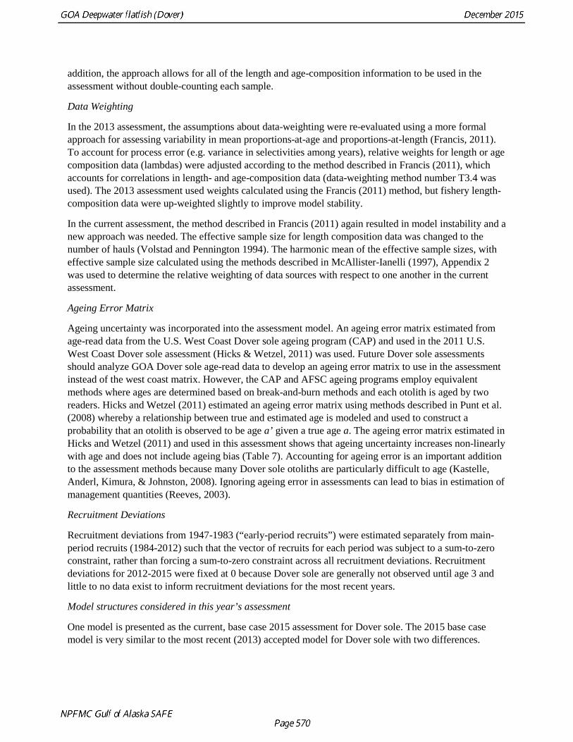
In the current assessment, the method described in Francis (2011) again resulted in model instability and a new approach was needed. The effective sample size for length composition data was changed to the number of hauls (Volstad and Pennington 1994). The harmonic mean of the effective sample sizes, with effective sample size calculated using the methods described in McAllister-Ianelli (1997), Appendix 2 was used to determine the relative weighting of data sources with respect to one another in the current assessment.

Ageing Error Matrix

Ageing uncertainty was incorporated into the assessment model. An ageing error matrix estimated from age-read data from the U.S. West Coast Dover sole ageing program (CAP) and used in the 2011 U.S. West Coast Dover sole assessment (Hicks & Wetzel, 2011) was used. Future Dover sole assessments should analyze GOA Dover sole age-read data to develop an ageing error matrix to use in the assessment instead of the west coast matrix. However, the CAP and AFSC ageing programs employ equivalent methods where ages are determined based on break-and-burn methods and each otolith is aged by two readers. Hicks and Wetzel (2011) estimated an ageing error matrix using methods described in Punt et al. (2008) whereby a relationship between true and estimated age is modeled and used to construct a probability that an otolith is observed to be age a’ given a true age a. The ageing error matrix estimated in Hicks and Wetzel (2011) and used in this assessment shows that ageing uncertainty increases non-linearly with age and does not include ageing bias (Table 7). Accounting for ageing error is an important addition to the assessment methods because many Dover sole otoliths are particularly difficult to age (Kastelle, Anderl, Kimura, & Johnston, 2008). Ignoring ageing error in assessments can lead to bias in estimation of management quantities (Reeves, 2003).

Recruitment Deviations

Recruitment deviations from 1947-1983 (“early-period recruits”) were estimated separately from main-period recruits (1984-2012) such that the vector of recruits for each period was subject to a sum-to-zero constraint, rather than forcing a sum-to-zero constraint across all recruitment deviations. Recruitment deviations for 2012-2015 were fixed at 0 because Dover sole are generally not observed until age 3 and little to no data exist to inform recruitment deviations for the most recent years.

Model structures considered in this year’s assessment

One model is presented as the current, base case 2015 assessment for Dover sole. The 2015 base case model is very similar to the most recent (2013) accepted model for Dover sole with two differences.

First, fishery selectivity is not allowed to be dome-shaped; the descending limb of the age-based male and female selectivity curves were fixed at a large number to force the curves to be asymptotic. This choice was made because the standard deviation for the descending limb parameter was very large (267.55 in log space in the 2013 model), both in the 2013 assessment and in model runs of the 2013 assessment with new data added, indicating that the data do not inform the model fit of the descending limb parameter and thus evidence for dome-shaped fishery selectivity is very weak. The catch of Dover sole is very small (Table 1, Figure 1) and therefore data informing fishery selectivity parameters are sparse.

Second, the data weighting approach was changed from the approach described in Francis (2011) to use of the harmonic mean of effective sample size, with effective sample size calculated according to methods described in McAllister and Ianelli (1997), Appendix 2. In addition the effective sample sizes assumed for each year of length composition data were changed to the number of hauls due to correlations within hauls, which was analyzed in Volstad and Pennington (1994). As described in the section on data weighting (above), the Francis (2011) approach created instability in the Dover sole model. It is possible that perceived process-related correlations in the fishery length composition data, as calculated by the Francis (2011) method, are just noise due to low sample size (given that catches are so low for Dover sole).

Parameters Estimated Outside the Assessment Model Natural Mortality

Natural mortality was fixed at 0.085. This value was used in previous accepted Dover sole assessment models (McGilliard et al. 2013) and was estimated using the Hoenig method (Hoenig, 1983). Natural mortality for GOA Dover sole should be re-evaluated in future GOA Dover sole assessments.

Weight-Length Relationship

The weight-length relationship used in the assessment was estimated for GOA Dover sole by Abookire and Macewicz (2003). The relationship was , where and , length (L) was measured in centimeters and weight (w) was measured in kilograms.

Maturity-at-Age

Maturity-at-age in the assessment was defined as , where the slope of the

curve was and the age-at-50%-maturity was .

A logistic maturity-at-length relationship estimated in Abookire and Macewicz (2003) was converted into a maturity-at-age relationship using the mean length-at-age relationship estimated within the assessment model. The maturity curve does not influence the estimation of the mean length-at-age relationship because spawning stock biomass (SSB) is the only quantity influenced by maturity in the model and SSB does not influence model fits because no stock-recruitment relationship is used.

A maturity-at-length curve was not used because slow growing fish in the model never become large enough to mature, regardless of age. This is unrealistic. Abookire and Macewicz (2003) estimated maturity-at-age as well as a maturity-at-length. However, the relatively low sample size of aged fish used in the Abookire and Macewicz (2003) study, combined with the large magnitude of ageing error known to exist for Dover sole suggested that the maturity-at-age relationship estimated in the paper may be unreliable.

Lw Lβα= 2.9 06Eα = − 3.3369β =

( )aO 50( )1/ (1 )a aaO eγ −= +

0.363γ = − 50 12.47a =

Standard deviation of the Log of Recruitment ( )

The standard deviation of the log of recruitment was not defined in previous assessments. Variability of the recruitment deviations that were estimated in previous Dover sole assessments was approximately =0.49 and this value was used in the current assessment.

Catchability

Catchability was equal to 1, as for previous Dover sole assessments. Future assessments should explore this assumption further.

Select selectivity parameters

Selectivity parameter definitions and values are shown in (Table 8).

Parameters Estimated Inside the Assessment Model Parameters estimated within the assessment model are the log of unfished recruitment (R0), log-scale recruitment deviations, yearly fishing mortality, sex-specific parameters of the von-Bertalanffy growth curve, CV of length-at-age for ages 2 and 59, and selectivity parameters for the fishery, the “full coverage” survey, and the “shallow-coverage” survey. The selectivity parameters are described in greater detail in Table 8).

Results

Model Evaluation Comparison of the current base case model to the 2013 model and variants

Figure 3-Figure 6 and Table 9 compare results of the current base case model to results from the 2013 model, as well as for the current base case model without 2014-2015 new data and the current base case model without 2014-2015 new data and with dome-shaped fishery selectivity estimated (as it was in the 2013 model). Fits to the survey biomass index are very similar among models (Figure 3). The survey biomass estimate for 2015 is the lowest on record (Figure 3, Table 6); none of the models fit the 2015 survey biomass estimate closely. Catches for 2014 and 2015 are not above average (Table 1 and Figure 1) and do not explain the low survey biomass that was observed in 2015.

The likelihood components for survey biomass were similar among base case models run without new data and for the 2013 model (Table 9). The likelihood component for survey biomass worsened with the addition of new data (Table 9) because fits to the 2015 survey biomass were poor (the survey biomass estimate was very low in 2015 and could not be fully explained by the model; Figure 3). In addition, survey, length, and age composition likelihood components for the base case model without new data and the base case model without new data and with dome-shaped fishery selectivity are very similar, indicating that estimating the descending limb of the fishery selectivity curve did not improve any likelihood components. Likelihood components from the 2015 base case model cannot be compared directly with likelihood components from models without new data. Also, likelihood components for length and age composition data from the 2013 model cannot be compared to other models because the effective sample sizes and data weighting differed.

Estimates of recruitment deviations are similar among models (Figure 4 and Figure 5). The 2013 model estimated a larger number of recruits in the early 2000s (Figure 5) than the other models, indicating that

Rσ

Rσ

the new data influenced the estimates of recruitment in those years. The 2015 model estimated a larger number of recent (2010-2012) recruits than the other models. However, little information is available on the number of recruits in 2010-2012, as the youngest Dover sole that are observed in the data are three years old and thus have only been observed for 0-2 years.

Estimated spawning stock biomass was lower in all years than for the 2013 model (Figure 6). The current base case model without new data and the current model without new data and with dome-shaped selectivity both yielded estimates of spawning stock biomass that were lower than for the 2013 model and higher than for the current model. The only difference between the 2013 model and the 2015 model with no new data and dome-shaped selectivity was the data weighting approach. Hence, the 2014-2015 data and the changes in data weights both influenced the estimates of spawning stock biomass over time (Figure 6). Model estimates of full-coverage survey selectivity differed among models (Figure 7). Both male and female selectivity increase at earlier ages than for the 2013 model, effectively creating an increase in catchability for the 2015 base case model, which then results in lower estimates of SSB in the 2015 base case model than for the 2013 model.

The Current Base Case Model

The estimated asymptotic fishery selectivity curves are shown in Figure 9 and selectivity for the full-coverage and shallow-coverage surveys are shown in Figure 10. Parameter estimates for the selectivity curves are shown in (Table 11). For the fishery and surveys, estimated selectivity occurs at smaller lengths and younger ages for males than for females. Further research could look into reasons for this pattern. The full-coverage survey selectivity was restricted to be asymptotic because the composition data associated with these survey years covered depths up to 1000 m and therefore (theoretically) all ages (Figure 10, Table 11). Age-based Dover sole selectivity was used because sensitivity analyses using length-based selectivity curves showed that the oldest Dover sole were never selected in the full coverage survey years (due to variability in length at older ages); this inadvertently decreased catchability in the model. Estimates of selectivity for the shallow-water survey were dome-shaped and suggest that females were more available to the fishery than males at most ages when only shallow depths were sampled (Figure 10, Table 11); this is consistent with tagging studies showing that female Dover sole may move between deeper and shallower depths more than males to spawn and feed (Demory et al., 1984; Westrheim et al., 1992). Estimates of selectivity for the shallow-water survey years correspond only to composition data and were not informed by an index of biomass.

Plots of observed and expected proportions-at-length aggregated over years are shown in Figure 11 and yearly fits to proportion-at-length data are shown in Figure 12-Figure 15. Fits to aggregated fishery and full-coverage survey proportions-at-length are very close to the observed values for females and males. Estimated aggregated proportions-at-length for the shallow water survey show that the model expected fewer 40-50cm females and fewer 35-45 cm males, but otherwise the estimated aggregated survey proportions-at-length were very close to the observed values (Figure 12).

Fits to conditional age-at-length data and variability in age-at-length are generally close to the observed mean length at age (Figure 16-Figure 18). Mean age-at-length observations do not always increase monotonically with length, indicating that data are variable. Expected standard deviation in age-at-length often diverges from observed standard deviation in age-at-length at large lengths because there are few data points observed (resulting in low observed standard deviations). Pearson residuals for conditional age-at-length fits are shown in Figure 19-Figure 21. Estimated values for growth parameters are shown in Table 9.

Time Series Results Time series results are shown in Table 14-Table 15 and Figure 22-Figure 23. A time series of numbers at age is available at (http://www.afsc.noaa.gov/REFM/Docs/2015/GOA_Dover_TimeSeries_of_NumbersAtAge_2015.xlsx). Age 3 recruitment, age 0 recruitment, and standard deviations of age 0 recruitment estimates are presented in Table 15 for the previous and current assessments. Total biomass for ages 3+, SSB, and standard deviations of SSB estimates for the previous and current assessments are presented in Table 14. Figure 22 shows SSB estimates and corresponding asymptotic 95% confidence intervals. Figure 23 is a plot of biomass relative to B35% and F relative to F35% for each year in the time series, along with the OFL and ABC control rules.

Retrospective analysis

Figure 24 and Figure 25 show the spawning stock biomass, recruitment deviations, and age-0 recruits for model runs excluding 0 to 10 years of data. Recruitment is assumed to be at its estimated mean value for years where data are excluded. Figure 24 appears to show a slight retrospective pattern for some model runs excluding 2015 data. However, the 2015 data has a large effect on the estimated spawning stock biomass. This is not surprising, given the low 2015 survey biomass estimate. Figure 25 shows that models excluding 0 to 10 years of data each estimate a large cohort of recruits in 1999 and again in 2001.

Harvest Recommendations Tier 3 Approach for Dover Sole

The reference fishing mortality rate for Dover sole is determined by the amount of reliable population information available (Amendment 56 of the Fishery Management Plan for the groundfish fishery of the GOA). Estimates of F40%, F35%, and SPR40% were obtained from a spawner-per-recruit analysis. Assuming that the average recruitment from the 1978-2012 year classes estimated in this assessment represents a reliable estimate of equilibrium recruitment, then an estimate of B40% can be calculated as the product of SPR40% times the equilibrium number of recruits. Since reliable estimates of the 2016 spawning biomass (B), B40%, F40%, and F35% exist and B>B40%, the Dover sole reference fishing mortality is defined in Tier 3a. For this tier, FABC is constrained to be ≤ F40%, and FOFL is defined to be F35%. The values of these quantities are:

SSB 2016 49,179 B40% 22,692 F40% 0.1 maxFABC 0.1 B35% 19,855 F35% 0.12 FOFL 0.12

Because the Dover sole stock has not been overfished in recent years and the stock biomass is relatively high, we do not recommended adjusting FABC downward from its upper bound of the maximum permissible FABC (maxFABC).

A standard set of projections is required for each stock managed under Tiers 1, 2, or 3 of Amendment 56. This set of projections encompasses seven harvest scenarios designed to satisfy the requirements of Amendment 56, the National Environmental Policy Act, and the MSFCMA. For each scenario, the projections begin with the vector of 2015 numbers-at-age estimated in the assessment. This vector is then projected forward to the beginning of 2028 using the schedules of natural mortality and selectivity described in the assessment and the best available estimate of total (year-end) catch for 2015. In each subsequent year, the fishing mortality rate is prescribed on the basis of the spawning biomass in that year and the respective harvest scenario. In each year, recruitment is drawn from an inverse Gaussian distribution whose parameters consist of maximum likelihood estimates determined from recruitments estimated in the assessment. Spawning biomass is computed in each year based on the time of peak spawning and the maturity and weight schedules described in the assessment. Total catch is assumed to equal the catch associated with the respective harvest scenario in all years. This projection scheme is run 1000 times to obtain distributions of possible future stock sizes, fishing mortality rates, and catches.

Five of the seven standard scenarios will be used in an Environmental Assessment prepared in conjunction with the final SAFE. These five scenarios, which are designed to provide a range of harvest alternatives that are likely to bracket the final TAC for 2016 and 2017, are as follow (“max FABC” refers to the maximum permissible value of FABC under Amendment 56):

Scenario 1: In all future years, F is set equal to max FABC. (Rationale: Historically, TAC has been constrained by ABC, so this scenario provides a likely upper limit on future TACs.)

Scenario 2: In all future years, F is set equal to a constant fraction of max FABC, where this fraction is equal to the ratio of the FABC value for 2016 recommended in the assessment to the maxFABC for 2016. (Rationale: When FABC is set at a value below max FABC, it is often set at the value recommended in the stock assessment.)

Scenario 3: In all future years, F is set equal to 50% of max FABC. (Rationale: This scenario provides a likely lower bound on FABC that still allows future harvest rates to be adjusted downward when stocks fall below reference levels.)

Scenario 4: In all future years, F is set equal to the 2011-2015 average F. (Rationale: For some stocks, TAC can be well below ABC, and recent average F may provide a better indicator of FTAC than FABC.)

Scenario 5: In all future years, F is set equal to zero. (Rationale: In extreme cases, TAC may be set at a level close to zero.)

The 12-year projections of the mean SSB, fishing mortality, and catches for the five scenarios are shown in Table 16-Table 18. The recommended FABC and the maximum FABC are equivalent in this assessment, so scenarios 1 and 2 yield identical results. Two other scenarios are needed to satisfy the MSFCMA’s requirement to determine whether the Dover sole stock is currently in an overfished condition or is approaching an overfished condition. These two scenarios are as follows (for Tier 3 stocks, the MSY level is defined as B35%):

Scenario 6: In all future years, F is set equal to FOFL. (Rationale: This scenario determines whether a stock is overfished. If the stock is expected to be 1) above its MSY level in 2015, or 2) above ½ of its MSY level in 2015 and expected to be above its MSY level in 2025 under this scenario, then the stock is not overfished.)

Scenario 7: In 2016 and 2017, F is set equal to maxFABC, and in all subsequent years, F is set equal to FOFL. (Rationale: This scenario determines whether a stock is approaching an overfished condition. If the stock is expected to be above its MSY level in 2028 under this scenario, then the stock is not approaching an overfished condition.)

The results of these two scenarios indicate that the stock is not overfished and is not approaching an overfished condition. With regard to assessing the current stock level, the expected stock size in the year 2015 of Scenario 6 is 48,918, more than 2 times B35% (19,855). Thus the stock is not currently overfished. With regard to whether the stock is approaching an overfished condition, the expected spawning stock size in the year 2028 of Scenario 7 (24,742) is greater than B35%; thus, the stock is not approaching an overfished condition.

Area Allocation for Harvests

ABCs and TACs for deepwater flatfish in the GOA are divided among four smaller management areas (Eastern, Central, West Yakutat and Southeast Outside). Area-specific ABCs are calculated as the total ABC multiplied by the proportion of deepwater flatfish survey biomass found in each area from 2005-2015.

Quantity Western Central West

Yakutat Southeast Total 2.0% 37.9% 32.5% 27.6% 100.0%

2016 ABC (t) 186 3,496 2,997 2,548 9,226 2017 ABC (t) 187 3,516 3,015 2,563 9,280

Ecosystem Considerations

Ecosystem Effects on the Stock Based on results from an ecosystem model for the GOA (Aydin et al., 2007), Dover sole adults occupy an intermediate trophic level (Figure 26 and Figure 27). Dover sole commonly feed on brittle stars, polychaetes and other miscellaneous worms (Figure 27; Buckley et al., 1999). Trends in prey abundance for Dover sole are unknown.

Important predators identified in the GOA ecosystem model include walleye pollock and Pacific halibut; however, the major source of Dover sole mortality is from the flatfish fishery (Figure 28). The ecosystem model was developed using food habits data from the early 1990s when GOA pollock biomass was much larger than it is currently and fishing mortality on Dover sole was much higher than it is now.

Little is known regarding the roles of Greenland turbot or deepsea sole in the GOA ecosystem. Within the 200-mile limits of the Exclusive Economic Zone of the United States, Greenland turbot are mainly found in the Bering Sea and the Aleutian Islands (Ianelli et al., 2006). Although the GOA component of Greenland turbot may represent a marginal stock, the species range in the eastern Pacific extends to northern Baja California. It thus seems somewhat unlikely that stock size in the GOA is limited by simple environmental factors such as temperature, rather it seems more likely that substantial biomass exists beyond the depth range of the fishery and the surveys. Greenland turbot are epibenthic feeders and prey on crustaceans and fishes. Walleye pollock are important predators on turbot in the Bering Sea, but it is unknown whether this holds true in the GOA as well.

Fishery Effects on the Ecosystem Table 19 shows the catch of non-target species in the deepwater flatfish fishery in recent years. In 2014, the deepwater flatfish fishery caught 100% of the lanternfish captured in GOA. In 2015, the deepwater flatfish fishery did not catch a substantial proportion of any of the non-target species. A table of the proportions of prohibited species catch taken in the deepwater flatfish fishery is not shown because values are currently confidential.

Data Gaps and Research Priorities The 2013 and 2015 stock assessment incorporated ageing error by using an existing ageing error matrix for West Coast Dover sole. A priority for future assessments is to analyze ageing error data for GOA Dover sole using methods described in Punt et al. (2008) and to incorporate a resulting ageing error matrix into the assessment. The assessment would benefit from an exploration of ways to better account for scientific uncertainty, especially uncertainty associated with parameters that are currently fixed in the model, including an exploration of natural mortality and catchability. The full coverage survey selectivity estimates indicate that males are selected at younger ages than females, which is counterintuitive. Future research could be done to explore this phenomenon.

Literature Cited Abookire, A. A., & Macewicz, B. J. (2003). Latitudinal variation in reproductive biology and growth of

female Dover sole (Microstomus pacificus) in the North Pacific, with emphasis on the Gulf of Alaska stock. Journal of Sea Research, 50, 187-197.

Demory, R. L., Golden, J. T., & Pikitch, E. (1984). Status of Dover sole (Microstomus pacificus) in INPFC Columbia and Vancouver areas in 1984. Status f Pacific Coast Groundfish Fishery and Recommendations for Management in 1985. Pacific Fishery Management Council. Portland, Oregon 97201.

Francis, R. I. C. C. (2011). Data weighting in statistical fisheries stock assessment models. Canadian Journal of Fisheries and Aquatic Sciences, 68, 1124-1138.

Hart, J. L. (1973). Pacific fishes of Canada. Fish Res. Board Canada, Bull. No. 180. 740 p. Hicks, A., & Wetzel, C. R. (2011). The Status of Dover Sole (Microstomus pacificus) along the U.S.

West Coast in 2011. Pacific Fishery Management Council. Portland, Oregon. www.pcouncil.org.

Hirschberger, W. A., & Smith, G. B. (1983). Spawning of twelve groundfish species in the Alaska and Pacific coast regions. 50 p. NOAA Tech. Mem. NMFS F/NWC-44. U.S> Dep. Commer., NOAA, Natl. Mar. Fish. Serv.

Hoenig, J. (1983). Empirical use of longevity data to estimate mortality rates. Fish Bulletin, 82, 898-903. Horn, & Francis, R. I. C. C. (2010). Stock assessment of hake (Merluccius australis) on the Chatham Rise

for the 2009–10 fishing year. New Zealand Fisheries Assessment Report 2010/14, Ministry of Fisheries, Wellington, New Zealand.

Hunter, J. R., Macewicz, B. J., Lo, N. C. H., & Kimbrell, C. A. (1992). Fecundity, spawning, and maturity of female Dover sole, Microstomus pacificus, with an evaluation of assumptions and precision. . Fish. Bull., 90, 101-128.

Kastelle, C. R., Anderl, D. M., Kimura, D. K., & Johnston, C. G. (2008). Age validation of Dover sole (Microstomus pacificus) by means of bomb radiocarbon. Fishery Bulletin, 106(4), 375-385.

Kendall, A. W. J., & Dunn, J. R. (1985). Ichthyoplankton of the continental shelf near Kodiak Island, Alaska. NOAA Tech. Rep. NMFS 20, U.S. Dep. Commer., NOAA, Natl. Mar. Fish. Serv.

Markle, D. F., Harris, P. M., & Toole, C. L. (1992). Metamorphosis and an overview of early life-history stages in Dover sole Microstomus pacificus. Fish Bulletin, 90, 285-301.

Martin, M. H., & Clausen, D. M. (1995). Data report: 1993 Gulf of Alaska Bottom Trawl Survey. U.S. Dept. Commer., NOAA, Natl. Mar. Fish. Serv., NOAA Tech. Mem. NMFS-AFSC-59, 217p.

McAllister, M.K. and Ianelli, J.N. 1997. Bayesian stock assessment using catch-age data and the sampling –importance resampling algorithm. Can. J. Fish. Aquat. Sci. 54: 284-300.

McGilliard, C.R., Palsson, W., Stockhausen, W., and Ianelli, J. 2013. 5. Assessment of the Deepwater Flatfish Stock in the Gulf of Alaska. In Stock Assessment and Fishery Evaluation Document for Groundfish Resources in the Gulf of Alaska as Projected for 2013. pp. 403-536.

Methot, R. D. (2009). User manual for stock synthesis, model version 3.04b. NOAA Fisheries, Seattle, WA.

Methot, R. D., & Wetzel, C. R. (2013). Stock synthesis: A biological and statistical framework for fish stock assessment and fishery management. Fisheries Research, 142, 86-99.

Miller, D. J., & Lea, R. N. (1972). Guide to the coastal marine fishes of California. Calif. Dept. Fish Game, Fish. Bull. 157, 235p., 157.

Pennington, M., & Volstad, J. H. (1994). Assessing the effect of intra-haul correlation and variable density on estimates of population characteristics from marine surveys. Biometrics, 50, 725-732.

Punt, A. E., Smith, D. C., KrusicGolub, K., & Robertson, S. (2008). Quantifying age-reading error for use in fisheries stock assessments, with application to species in Australia's southern and eastern scalefish and shark fishery. Canadian Journal of Fisheries and Aquatic Sciences, 65(9), 1991-2005. doi: 10.1139/f08-111

Reeves, S. A. (2003). A simulation study of the implications of age-reading errors for stock assessment and management advice. Ices Journal of Marine Science, 60, 314-328.

Stewart, I. J. (2005). Status of the U.S. English sole resource in 2005. Pacific Fishery Management Council. Portland, Oregon. www.pcouncil.org. 221 p. .

Stockhausen, W. T., Wilkins, M. E., & Martin, M. H. (2011). 5. Assessment of the Deepwater Flatfish Stock in the Gulf of Alaska. In Stock Assessment and Fishery Evaluation Document for Groudfish Resources in the Gulf of Alaska as Projected for 2012. pp. 547-628. North Pacific Fishery Management Council, P.O. Box 103136, Anchorage, AK 99510.

Turnock, B. J., Wilderbuer, T. K., & Brown, E. S. (2003). Gulf of Alaska Dover sole. In Stock Assessment and Fishery Evaluation Document for Groundfish Resources in the Gulf of Alaska as Projected for 2004. pp. 341-368. North Pacific Fishery Management Council, P.O. Box 103136, Anchorage AK 99510.

Wakabayashi, K., Bakkala, R.G. , and Alton, M.S. (1985). Methods of the U.S.-Japan demersal trawl surveys. In Richard G. Bakkala and Kiyoshi Wakabayashi (editors), Results of cooperative U.S.-Japan groundfish investigations in the Bering Sea during May-August 1979, p. 7-29. . Int. North Pac. Fish. Comm. Bull., 44.

Westrheim, S. J., Barss, W. H., Pikitch, E. K., & Quirollo, L. F. (1992). Stock Delineation of Dover Sole in the California-British Columbia Region, Based on Tagging Studies Conducted during 1948-1979. North American Journal of Fisheries Management 12:172-181.

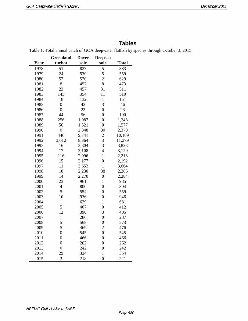
Tables Table 1. Total annual catch of GOA deepwater flatfish by species through October 3, 2015.

Year Greenland

turbot Dover

sole Deepsea

sole Total 1978 51 827 5 883 1979 24 530 5 559 1980 57 570 2 629 1981 8 457 8 473 1982 23 457 31 511 1983 145 354 11 510 1984 18 132 1 151 1985 0 43 3 46 1986 0 23 0 23 1987 44 56 0 100 1988 256 1,087 0 1,343 1989 56 1,521 0 1,577 1990 0 2,348 30 2,378 1991 446 9,741 2 10,189 1992 3,012 8,364 3 11,379 1993 16 3,804 3 3,823 1994 17 3,108 4 3,129 1995 116 2,096 1 2,213 1996 15 2,177 0 2,192 1997 11 3,652 1 3,664 1998 18 2,230 38 2,286 1999 14 2,270 0 2,284 2000 23 961 1 985 2001 4 800 0 804 2002 5 554 0 559 2003 10 936 0 946 2004 1 679 1 681 2005 5 407 0 412 2006 12 390 3 405 2007 1 286 0 287 2008 5 568 0 573 2009 5 469 2 476 2010 0 545 0 545 2011 0 466 0 466 2012 0 262 0 262 2013 0 242 0 242 2014 29 324 1 354 2015 3 218 0 221

Table 2. Historical OFLs, ABCs, TACs, and the percent of catch retained each year.

Year OFL ABC TAC Percent

Retained 1995 17,040 14,590 11,080 79% 1996 17,040 14,590 11,080 72% 1997 9,440 7,170 7,170 82% 1998 9,440 7,170 7,170 90% 1999 8,070 6,050 6,050 80% 2000 6,980 5,300 5,300 71% 2001 6,980 5,300 5,300 75% 2002 6,430 4,880 4,880 64% 2003 6,430 4,880 4,880 50% 2004 8,010 6,070 6,070 81% 2005 8,490 6,820 6,820 42% 2006 11,008 8,665 8,665 40% 2007 10,431 8,707 8,707 41% 2008 11,343 8,903 8,903 37% 2009 11,578 9,168 9,168 21% 2010 7,680 6,190 6,190 61% 2011 7,823 6,305 6,305 51% 2012 6,834 5,126 5,126 25% 2013 6,834 5,126 5,126 61% 2014 16,159 13,472 13,472 24% 2015 15,993 13,334 13,334 47%

Table 3. 2015 closures of the GOA deepwater flatfish fishery Sub-Area Program Status Reason Effective

Date

GOA - Central 620/630 All Bycatch Regulations 01-Jan

GOA - Western 610 All Bycatch Regulations 01-Jan

GOA - Central 620/630 All Open Regulations 20-Jan

GOA - Western 610 All Open Regulations 20-Jan

West Yakutat - 640 All Open Regulations 20-Jan

West Yakutat - 640 All Bycatch Regulations 01-Jan

GOA - Central 620/630 Catcher Vessel

Bycatch Chinook Salmon

03-May

GOA - Western 610 Catcher Vessel

Bycatch Chinook Salmon

03-May

GOA - Central 620/630 Catcher Vessel

Open Regulations 10-Aug

GOA - Western 610 Catcher Vessel

Open Regulations 10-Aug

Table 4. Survey biomass by depth and area Depth (meters) 1-100 101-200 201-300 301-500 501-700 701-1000 CENTRAL GOA 42,328 265,732 134,787 53,187 35,516 19,128

1984 1,870 24,506 5,598 4,039 5,147 11,309 1987 1,260 12,728 8,587 3,706 6,757 1,539 1990 11,233 42,188 15,644 2,043 1993 3,937 24,054 10,883 4,640 1996 1,674 21,452 8,691 5,327 1999 3,619 14,068 8,085 4,779 2,889 716 2001 3,785 16,241 7,303 4,200 2003 2,842 23,005 10,070 4,629 8,738 2005 4,255 19,805 6,691 4,742 1,617 1,772 2007 1,748 22,417 9,543 4,437 3,604 1,655 2009 2,372 15,668 12,619 3,158 1,769 236 2011 1,810 14,528 15,131 2,578 1,501 2013 1,196 7,789 9,896 2,026 2,273 2015 728 7,284 6,044 2,885 1,222 1,901

EASTERN GOA 54,946 161,580 105,826 115,897 20,119 1,736 1984 925 4,989 1,975 1,645 1,728 330 1987 3,137 12,995 3,419 4,126 2,518 1990 896 14,869 4,290 3,784 1993 651 18,901 8,893 11,219 1996 4,753 16,066 9,121 10,988 1999 2,806 14,425 11,448 6,887 2,476 606 2003 7,119 21,636 7,491 8,153 2,466 2005 1,924 12,340 10,732 12,577 1,206 69 2007 903 6,887 9,945 6,430 1,298 278 2009 4,008 10,253 10,979 5,595 4,144 411 2011 2,377 10,065 11,102 16,704 902 2013 23,355 7,928 11,178 14,994 1,125 2015 2,094 10,225 5,254 12,796 2,256 42

WESTERN GOA 1,665 5,875 2,023 8,606 9,319 2,930 1984 34 725 355 1,138 1,290 919 1987 5 108 32 1,103 1,267 108 1990 161 716 50 721 1993 172 1,044 154 1,001 1996 134 337 290 698 1999 7 56 43 651 685 0 2001 18 53 188 636 2003 194 541 270 811 1,333 2005 475 468 275 455 312 848 2007 78 405 110 468 208 1,056 2009 154 565 88 548 3,712 0 2011 235 146 8 134 311 2013 0 627 126 84 142 2015 0 85 34 157 60 0

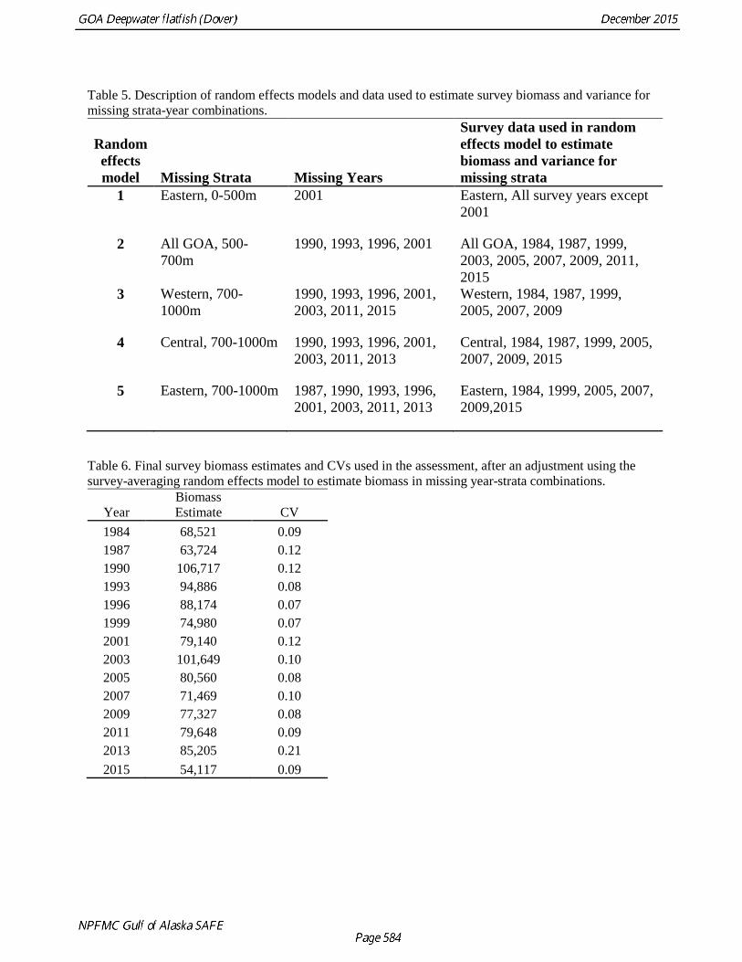
Table 5. Description of random effects models and data used to estimate survey biomass and variance for missing strata-year combinations.

Random effects model Missing Strata Missing Years

Survey data used in random effects model to estimate biomass and variance for missing strata

1 Eastern, 0-500m 2001 Eastern, All survey years except 2001

2 All GOA, 500-700m

1990, 1993, 1996, 2001 All GOA, 1984, 1987, 1999, 2003, 2005, 2007, 2009, 2011, 2015

3 Western, 700-1000m

1990, 1993, 1996, 2001, 2003, 2011, 2015

Western, 1984, 1987, 1999, 2005, 2007, 2009

4 Central, 700-1000m 1990, 1993, 1996, 2001, 2003, 2011, 2013

Central, 1984, 1987, 1999, 2005, 2007, 2009, 2015

5 Eastern, 700-1000m 1987, 1990, 1993, 1996, 2001, 2003, 2011, 2013

Eastern, 1984, 1999, 2005, 2007, 2009,2015

Table 6. Final survey biomass estimates and CVs used in the assessment, after an adjustment using the survey-averaging random effects model to estimate biomass in missing year-strata combinations.

Year Biomass Estimate CV

1984 68,521 0.09 1987 63,724 0.12 1990 106,717 0.12 1993 94,886 0.08 1996 88,174 0.07 1999 74,980 0.07 2001 79,140 0.12 2003 101,649 0.10 2005 80,560 0.08 2007 71,469 0.10 2009 77,327 0.08 2011 79,648 0.09 2013 85,205 0.21 2015 54,117 0.09

Table 7. Ageing error uncertainty assumed in the assessment model.

True Age

Standard Deviation

True Age

Standard Deviation

0 0.210 30 4.224 1 0.210 31 4.464 2 0.284 32 4.715 3 0.361 33 4.975 4 0.441 34 5.247 5 0.525 35 5.530 6 0.612 36 5.824 7 0.703 37 6.131 8 0.797 38 6.450 9 0.896 39 6.783 10 0.998 40 7.129 11 1.105 41 7.490 12 1.216 42 7.866 13 1.332 43 8.257 14 1.452 44 8.664 15 1.578 45 9.089 16 1.709 46 9.531 17 1.845 47 9.991 18 1.987 48 10.470 19 2.134 49 10.969 20 2.288 50 11.489 21 2.448 51 12.031 22 2.615 52 12.594 23 2.789 53 13.182 24 2.970 54 13.793 25 3.158 55 14.430 26 3.354 56 15.093 27 3.559 57 15.784 28 3.771 58 16.503 29 3.993 59 17.252

Table 8. Estimated and fixed double-normal selectivity parameters. “Estimated” indicates that the parameter was estimated within the assessment and a numeric value indicates a fixed parameter value.

Double-normal selectivity parameters Fishery

"Full-coverage"

Survey "Shallow-

coverage" Survey

Peak: beginning size for the plateau (in cm) Estimated Estimated Estimated

Width: width of plateau 0 8 Estimated

Ascending width (log space) Estimated Estimated Estimated

Descending width (log space) 10 8 Estimated Initial: selectivity at smallest length or age bin -10 -10 Estimated

Final: selectivity at largest length or age bin 999 999 Estimated Male Peak Offset Estimated Estimated Estimated

Male ascending width offset (log space) Estimated Estimated Estimated

Male descending width offset (log space) 0 0 Estimated Male "Final" offset (transformation required) 0 0 Estimated Male apical selectivity 1 1 Estimated

Table 9. Negative log likelihood components for the 2015 base case model, the base case model without new data (data are as for the 2013 model), the base case model without new data and with dome-shaped selectivity, and the 2013 model. Values for likelihood components for the 2015 base case model cannot be compared directly with the other models. Only the value for the survey index likelihood component can be compared between the models using data up to 2013 because effective sample sizes, data weights, and the estimation of the most recent recruitment deviations differ between models.

Likelihood Component

2015 Base Case

Base Case w/o new

data

Base case w/o new data and w/

dome-shaped selectivity

2013 Base Case

TOTAL 1,423.78 1,249.07 1,248.87 3,410.61 Survey -4.13 -11.23 -11.12 -11.43 Length_comp 393.51 330.57 330.15 644.75 Age_comp 1,025.87 922.55 922.68 2,764.74 Recruitment 8.49 7.15 7.12 12.51

Table 10. Final parameter estimates of growth and unfished recruitment parameters with corresponding standard deviations for the current base case model for females (f) and males (m). “Std. Dev” is the standard deviation of the estimate.

Parameter Estimate Std. Dev.

Length at age 2 (f) 25.366 0.624

Linf (f) 52.101 0.451

von Bertalanffy k (f) 0.113 0.007

CV in length at age 2 (f) 0.150 0.010

CV in length at age 59 (f) 0.107 0.004

Length at age 2 (m) 27.110 0.695

Linf (m) 43.968 0.277

von Bertalanffy k (m) 0.158 0.013

CV in length at age 2 (m) 0.151 0.010

CV in length at age 59 (m) 0.090 0.003

R0 (log space) 9.876 0.046

Table 11. Final fishery, full coverage survey, and shallow coverage selectivity parameters for the current base case model. “Est” refers to the estimated value and “Std. Dev” is the standard deviation of the estimate.

Fishery Full Coverage

Survey Shallow Coverage

Survey

Double-normal selectivity parameters Est Std. Dev. Est

Std. Dev. Est Std. Dev.

Peak: beginning size for the plateau 48.81 1.27 45.00 0.09 23.16 1.80

Width: width of plateau Fixed Fixed -0.28 0.25

Ascending width (log space) 4.26 0.24 11.96 1.21 5.06 0.22

Descending width (log space) Fixed Fixed -0.73 14.80

Initial: selectivity at smallest length or age bin Fixed Fixed -498 11236.20

Final: selectivity at largest length or age bin Fixed Fixed -4.99 0.44 Male Peak Offset -9.28 1.37 -13.35 1.41 -15.00 0.05

Male ascending width offset (log space) -1.46 0.37 4.68 119.24 -2.74 0.65

Male descending width offset (log space) Fixed Fixed 3.75 14.12 Male "Final" offset (transformation required) Fixed Fixed 0.03 0.88 Male apical selectivity Fixed Fixed 0.58 0.06

Table 12. Estimated recruitment deviations and associated standard deviations for the current model. “Std. Dev” is the standard deviation of the estimate.

Year Recruitment Deviations

Std. Dev.

Year Recruitment Deviations

Std. Dev.

1947 -0.107 0.463 1981 0.206 0.472 1948 -0.113 0.462 1982 0.300 0.497 1949 -0.118 0.460 1983 0.683 0.461 1950 -0.124 0.462 1984 0.430 0.432 1951 -0.140 0.456 1985 -0.003 0.415 1952 -0.137 0.456 1986 0.418 0.323 1953 -0.133 0.462 1987 0.001 0.380 1954 -0.140 0.455 1988 -0.040 0.351 1955 -0.119 0.458 1989 -0.249 0.337 1956 -0.085 0.479 1990 -0.357 0.352 1957 0.011 0.486 1991 0.053 0.292 1958 0.085 0.501 1992 -0.290 0.338 1959 0.175 0.523 1993 -0.166 0.360 1960 0.272 0.550 1994 0.194 0.347 1961 0.360 0.578 1995 0.195 0.345 1962 0.407 0.596 1996 -0.028 0.369 1963 0.395 0.591 1997 -0.256 0.324 1964 0.340 0.570 1998 -0.492 0.352 1965 0.278 0.548 1999 1.292 0.161 1966 0.229 0.531 2000 -0.202 0.393 1967 0.188 0.517 2001 0.863 0.172 1968 0.143 0.504 2002 -0.805 0.332 1969 0.094 0.490 2003 0.212 0.234 1970 0.045 0.478 2004 -0.216 0.327 1971 0.000 0.467 2005 0.274 0.246 1972 -0.033 0.460 2006 -0.619 0.329 1973 -0.045 0.457 2007 -0.068 0.263 1974 -0.020 0.460 2008 -0.691 0.320 1975 0.061 0.475 2009 -0.375 0.325 1976 0.223 0.506 2010 -0.466 0.376 1977 0.448 0.535 2011 0.910 0.409 1978 0.417 0.531 2012 0.764 0.510 1979 0.207 0.494 2013 -0.283 0.390 1980 0.165 0.473

Table 13. Estimated fishing mortality rates for the current model. “Std. Dev” is the standard deviation of the estimate.

Year Fishing

Mortality Std. Dev. Year

Fishing Mortality

Std. Dev.

Initial F 0.0058 0.0003 1998 0.0254 0.0009

1978 0.0081 0.0005 1999 0.0263 0.0009 1979 0.0052 0.0003 2000 0.0113 0.0004 1980 0.0056 0.0003 2001 0.0094 0.0003 1981 0.0045 0.0002 2002 0.0065 0.0002 1982 0.0044 0.0002 2003 0.0110 0.0004 1983 0.0034 0.0002 2004 0.0079 0.0003 1984 0.0013 0.0001 2005 0.0047 0.0002 1985 0.0004 0.0000 2006 0.0044 0.0002 1986 0.0002 0.0000 2007 0.0031 0.0001 1987 0.0005 0.0000 2008 0.0061 0.0002 1988 0.0100 0.0004 2009 0.0050 0.0002 1989 0.0139 0.0006 2010 0.0058 0.0002 1990 0.0215 0.0009 2011 0.0049 0.0002 1991 0.0921 0.0036 2012 0.0027 0.0001 1992 0.0836 0.0032 2013 0.003 0.000 1993 0.0394 0.0015 2014 0.003 0.000 1994 0.0328 0.0012 2015 0.002 0.000 1995 0.0225 0.0008 1996 0.0237 0.0008 1997 0.0406 0.0014

Table 14. Time series of age 3+ total biomass, spawning biomass, and standard deviation of spawning biomass for the 2013 assessment and this year’s assessment. “Stdev_SPB” is the standard deviation of the estimate of spawning biomass.

2013 Assessment 2015 Assessment

Year

Total Biomass (age 3+)

Spawning Biomass Stdev_SPB

Total Biomass (age 3+)

Spawning Biomass Stdev_SPB

1978 150,904 68,209 4,072 120,778 51,020 3,107 1979 185,711 69,750 3,989 134,217 51,407 3,045 1980 185,077 71,027 3,892 134,229 51,802 2,971 1981 184,742 71,905 3,783 135,421 52,070 2,886 1982 184,336 72,470 3,670 136,746 52,284 2,794 1983 183,944 72,729 3,555 137,648 52,424 2,696 1984 183,503 72,795 3,443 138,410 52,565 2,595 1985 183,358 72,796 3,338 139,318 52,791 2,495 1986 184,127 72,762 3,242 140,679 53,095 2,392 1987 186,554 72,706 3,155 143,724 53,454 2,292 1988 188,222 72,661 3,079 146,052 53,857 2,195 1989 189,251 72,278 3,013 147,024 53,942 2,096 1990 189,456 71,833 2,961 148,060 53,925 2,002 1991 189,393 71,174 2,923 147,451 53,649 1,909 1992 187,522 67,776 2,888 145,726 50,560 1,787 1993 177,928 65,059 2,876 136,787 48,081 1,684 1994 168,975 64,190 2,886 128,845 47,410 1,612 1995 164,339 63,574 2,906 125,731 46,984 1,550 1996 159,389 63,278 2,932 122,511 46,901 1,500 1997 155,549 62,812 2,960 120,281 46,702 1,461 1998 152,196 61,559 2,988 118,793 45,791 1,430 1999 147,904 60,684 3,012 116,188 45,337 1,412 2000 144,763 59,612 3,032 114,512 44,740 1,401 2001 142,898 58,946 3,049 112,363 44,576 1,395 2002 142,716 58,321 3,070 110,906 44,486 1,393 2003 147,785 57,781 3,094 116,657 44,417 1,391 2004 151,086 57,174 3,131 117,503 44,244 1,391 2005 153,738 56,874 3,187 121,498 44,195 1,393 2006 157,353 56,939 3,268 121,783 44,358 1,400 2007 161,071 57,353 3,383 123,584 44,624 1,413 2008 167,239 58,116 3,532 124,228 45,064 1,433 2009 171,218 59,090 3,716 125,778 45,495 1,463 2010 173,726 60,361 3,931 125,144 46,072 1,503 2011 175,221 61,765 4,170 125,025 46,670 1,552 2012 174,950 63,279 4,422 123,584 47,300 1,608 2013 173,853 64,776 4,673 122,244 47,939 1,666 2014 182,727 66,147 0 120,702 48,516 1,726 2015 123,619 48,918 1,782 2016 141,926 49,180 0

Table 15. Time series of age 3 and age 0 recruits and standard deviation of age 0 recruits for the previous and current assessment models. “Std. dev” is the standard deviation of the estimate of Age 0 recruits.

2013 Assessment 2015 Assessment

Year Recruits (Age 3)

Recruits (Age 0) Std. dev

Recruits (Age 3)

Recruits (Age 0) Std. dev

1978 21,119 28,539 11,024 16,025 29,490 15,584 1979 21,119 27,002 11,028 18,841 23,807 11,720 1980 21,162 26,758 11,158 23,597 22,749 10,716 1981 22,452 29,477 12,565 22,852 23,592 11,090 1982 21,242 35,723 15,951 18,449 25,838 12,820 1983 21,051 41,973 17,258 17,628 37,721 17,055 1984 23,190 29,830 12,265 18,281 29,205 12,768 1985 28,103 21,826 8,415 20,022 18,855 7,899 1986 33,021 26,159 9,082 29,231 28,628 9,151 1987 23,467 28,067 8,488 22,632 18,791 7,177 1988 17,171 17,985 5,537 14,611 17,966 6,308 1989 20,579 12,330 3,614 22,184 14,524 4,924 1990 22,081 11,107 3,272 14,561 12,981 4,617 1991 14,149 18,392 4,068 13,922 19,497 5,662 1992 9,700 10,716 3,126 11,255 13,788 4,695 1993 8,738 18,305 4,584 10,059 15,540 5,618 1994 14,469 25,201 6,135 15,108 22,192 7,662 1995 8,430 24,962 6,233 10,684 22,122 7,622 1996 14,401 18,435 5,717 12,042 17,638 6,534 1997 19,826 30,834 7,544 17,196 13,993 4,582 1998 19,638 30,254 8,178 17,143 11,008 3,946 1999 14,503 81,845 12,167 13,668 65,463 10,035 2000 24,257 26,127 6,716 10,843 14,696 5,896 2001 23,801 21,324 5,690 8,530 42,611 7,319 2002 64,388 35,127 7,706 50,728 8,036 2,727 2003 20,554 34,510 9,091 11,388 22,223 5,218 2004 16,775 65,198 12,566 33,020 14,484 4,797 2005 27,635 23,449 7,108 6,227 23,644 5,831 2006 27,149 17,518 5,337 17,221 9,683 3,243 2007 51,291 18,156 5,398 11,224 16,798 4,464 2008 18,448 10,803 3,764 18,322 9,103 2,972 2009 13,782 16,263 6,442 7,503 12,625 4,179 2010 14,283 23,651 9,849 13,017 11,648 4,468 2011 8,499 26,619 11,407 7,054 46,614 18,935 2012 12,794 24,106 10,589 9,783 40,703 20,978 2013 21,163 29,542 9,026 14,435 5,777 2014 36,122 19,452 889 2015 31,541 19,452

Average 21,234 26,892 17,409 21,884

Table 16. Projected spawning biomass for the seven harvest scenarios listed in the “Harvest Recommendations” section.

Year Scenario 1 Scenario 2 Scenario 3 Scenario 4 Scenario 5 Scenario 6 Scenario 7 2015 48,918 48,918 48,918 48,918 48,918 48,918 48,918 2016 49,179 49,179 49,179 49,179 49,179 49,179 49,179 2017 49,271 49,271 49,271 49,271 49,271 44,933 45,680 2018 45,678 45,678 49,291 48,474 49,416 41,103 42,454 2019 42,435 42,435 49,278 47,682 49,525 37,730 38,918 2020 39,586 39,586 49,293 46,962 49,657 34,838 35,877 2021 37,158 37,158 49,393 46,370 49,869 32,432 33,336 2022 35,141 35,141 49,615 45,942 50,200 30,482 31,265 2023 33,496 33,496 49,971 45,683 50,660 28,930 29,604 2024 32,157 32,157 50,440 45,566 51,230 27,695 28,274 2025 31,047 31,047 50,979 45,543 51,867 26,692 27,186 2026 30,096 30,096 51,535 45,563 52,519 25,847 26,267 2027 29,253 29,253 52,063 45,581 53,140 25,107 25,462 2028 28,488 28,488 52,535 45,569 53,700 24,443 24,742

Table 17. Projected fishing mortality rates for the seven harvest scenarios listed in the “Harvest Recommendations” section.

Year Scenario 1 Scenario 2 Scenario 3 Scenario 4 Scenario 5 Scenario 6 Scenario 7 2015 0.00 0.00 0.00 0.00 0.00 0.00 0.00 2016 0.00 0.00 0.00 0.00 0.00 0.12 0.10 2017 0.10 0.10 0.00 0.02 0.00 0.12 0.10 2018 0.10 0.10 0.00 0.02 0.00 0.12 0.12 2019 0.10 0.10 0.00 0.02 0.00 0.12 0.12 2020 0.10 0.10 0.00 0.02 0.00 0.12 0.12 2021 0.10 0.10 0.00 0.02 0.00 0.12 0.12 2022 0.10 0.10 0.00 0.02 0.00 0.12 0.12 2023 0.10 0.10 0.00 0.02 0.00 0.12 0.12 2024 0.10 0.10 0.00 0.02 0.00 0.12 0.12 2025 0.10 0.10 0.00 0.02 0.00 0.12 0.12 2026 0.10 0.10 0.00 0.02 0.00 0.12 0.12 2027 0.10 0.10 0.00 0.02 0.00 0.12 0.12 2028 0.10 0.10 0.00 0.02 0.00 0.12 0.12

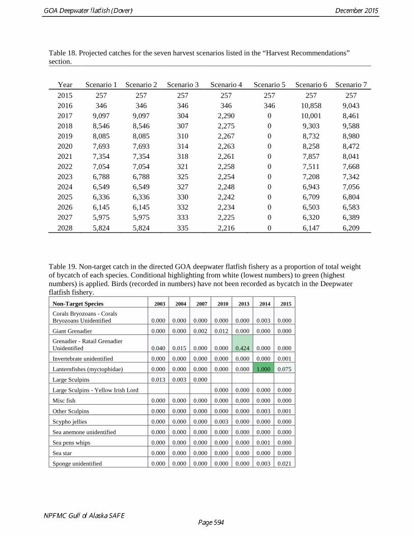
Table 18. Projected catches for the seven harvest scenarios listed in the “Harvest Recommendations” section.

Year Scenario 1 Scenario 2 Scenario 3 Scenario 4 Scenario 5 Scenario 6 Scenario 7 2015 257 257 257 257 257 257 257 2016 346 346 346 346 346 10,858 9,043 2017 9,097 9,097 304 2,290 0 10,001 8,461 2018 8,546 8,546 307 2,275 0 9,303 9,588 2019 8,085 8,085 310 2,267 0 8,732 8,980 2020 7,693 7,693 314 2,263 0 8,258 8,472 2021 7,354 7,354 318 2,261 0 7,857 8,041 2022 7,054 7,054 321 2,258 0 7,511 7,668 2023 6,788 6,788 325 2,254 0 7,208 7,342 2024 6,549 6,549 327 2,248 0 6,943 7,056 2025 6,336 6,336 330 2,242 0 6,709 6,804 2026 6,145 6,145 332 2,234 0 6,503 6,583 2027 5,975 5,975 333 2,225 0 6,320 6,389 2028 5,824 5,824 335 2,216 0 6,147 6,209

Table 19. Non-target catch in the directed GOA deepwater flatfish fishery as a proportion of total weight of bycatch of each species. Conditional highlighting from white (lowest numbers) to green (highest numbers) is applied. Birds (recorded in numbers) have not been recorded as bycatch in the Deepwater flatfish fishery.

Non-Target Species 2003 2004 2007 2010 2013 2014 2015

Corals Bryozoans - Corals Bryozoans Unidentified 0.000 0.000 0.000 0.000 0.000 0.003 0.000

Giant Grenadier 0.000 0.000 0.002 0.012 0.000 0.000 0.000

Grenadier - Ratail Grenadier Unidentified 0.040 0.015 0.000 0.000 0.424 0.000 0.000

Invertebrate unidentified 0.000 0.000 0.000 0.000 0.000 0.000 0.001

Lanternfishes (myctophidae) 0.000 0.000 0.000 0.000 0.000 1.000 0.075

Large Sculpins 0.013 0.003 0.000

Large Sculpins - Yellow Irish Lord 0.000 0.000 0.000 0.000

Misc fish 0.000 0.000 0.000 0.000 0.000 0.000 0.000

Other Sculpins 0.000 0.000 0.000 0.000 0.000 0.003 0.001

Scypho jellies 0.000 0.000 0.000 0.003 0.000 0.000 0.000

Sea anemone unidentified 0.000 0.000 0.000 0.000 0.000 0.000 0.000

Sea pens whips 0.000 0.000 0.000 0.000 0.000 0.001 0.000

Sea star 0.000 0.000 0.000 0.000 0.000 0.000 0.000

Sponge unidentified 0.000 0.000 0.000 0.000 0.000 0.003 0.021

Figures

Figure 1. Catch biomass of Dover sole in metric tons 1978-2015 (as of October 10, 2015).

Figure 2. Maps of survey catch-per-unit-effort (CPUE) from the 2015, 2013, and 2011 GOA Groundfish Trawl Survey.

Figure 3. Survey biomass index (black dots), asymptotic 95% confidence intervals (vertical black lines), and estimated survey biomass for the current base case model (blue), the base case model with new data removed (data up to 2013 only; green), the base case model with new data removed and dome-shaped selectivity (yellow), and the 2013 model (red).

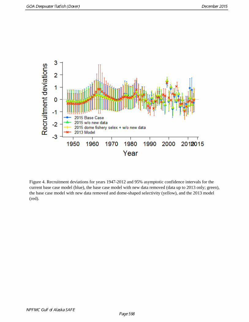
Figure 4. Recruitment deviations for years 1947-2012 and 95% asymptotic confidence intervals for the current base case model (blue), the base case model with new data removed (data up to 2013 only; green), the base case model with new data removed and dome-shaped selectivity (yellow), and the 2013 model (red).

Figure 5. Time series of age 0 recruits for the current base case model (blue), the base case model with new data removed (data up to 2013 only; green), the base case model with new data removed and dome-shaped selectivity (yellow), and the 2013 model (red).

Figure 6. Time series of spawning biomass and 95% asymptotic confidence intervals for the current base case model (blue), the base case model with new data removed (data up to 2013 only; green), the base case model with new data removed and dome-shaped selectivity (yellow), and the 2013 model (red).

Figure 7. Selectivity-at-age for the full coverage (top panel) and shallow coverage (bottom panel) surveys for the 2015 base case model, the 2015 model without new data (data is as for the 2013 model), the 2015 model without new data and with dome-shaped selectivity, and the 2013 model for females (left panel) and males (right panel).

Figure 8. Estimated mean length-at-age (solid lines) and variability about the length at age curve (dashed lines) defined by the estimated CVs of length at age 2 and 59 for females (red) and males (blue) for the current base case model.

Figure 9. Sex-specific, length-based, asymptotic fishery selectivity for the current base case model for females (solid line) and males (dashed lines).

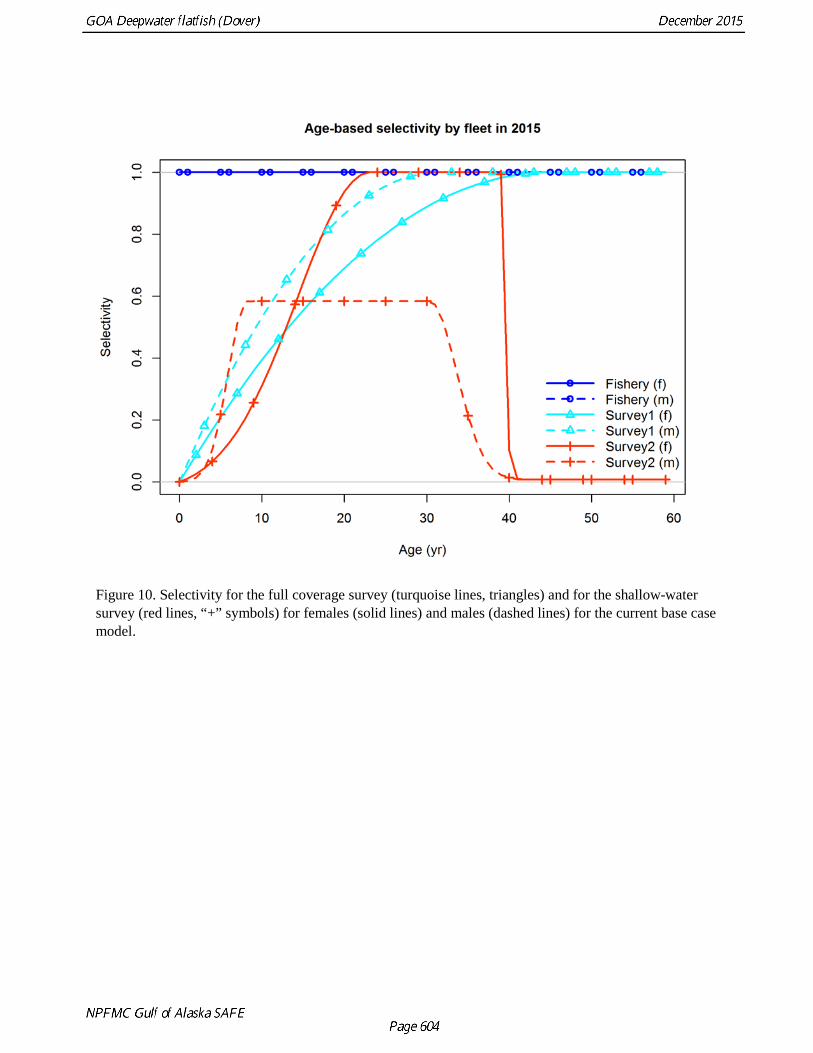
Figure 10. Selectivity for the full coverage survey (turquoise lines, triangles) and for the shallow-water survey (red lines, “+” symbols) for females (solid lines) and males (dashed lines) for the current base case model.

Figure 11. Observed (black lines, dots, and shaded areas) and expected (red lines) proportions-at-length, aggregated over years for the fishery, the full coverage survey, and the shallow coverage survey for the current base case model.

Figure 12. Observed (black lines, dots, and shaded areas) and expected (red and blue lines) yearly fishery proportions-at-length for the current base case model for years 1991-2010. Females are plotted above the x-axis; males are plotted below the x-axis.

Figure 13. As for Figure 12 for years 2011-2015.

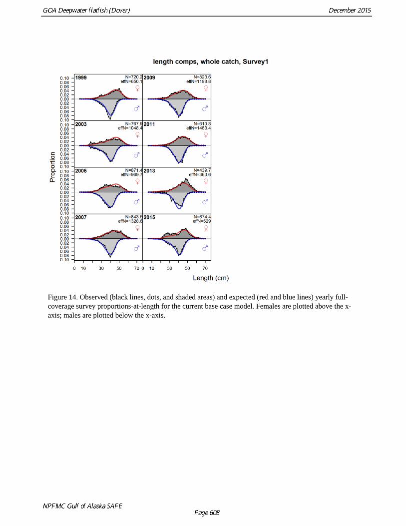
Figure 14. Observed (black lines, dots, and shaded areas) and expected (red and blue lines) yearly full-coverage survey proportions-at-length for the current base case model. Females are plotted above the x-axis; males are plotted below the x-axis.

Figure 15. Observed (black lines, dots, and shaded areas) and expected (red and blue lines) yearly shallow coverage survey proportions-at-length for the current base case model. Females are plotted above the x-axis; males are plotted below the x-axis.

Figure 16. Observed and expected mean age-at-length for males and females combined with 90% intervals about observed age-at-length (left panels) and observed and expected standard deviation in age-at-length (right panels) for the full coverage survey (1 of 2).

Length (cm)

Figure 17. Observed and expected mean age-at-length for males and females combined with 90% intervals about observed age-at-length (left panels) and observed and expected standard deviation in age-at-length (right panels) for the full coverage survey (2 of 2).

Figure 18. Observed and expected mean age-at-length for males and females combined with 90% intervals about observed age-at-length (left panels) and observed and expected standard deviation in age-at-length (right panels) for the shallow coverage survey.

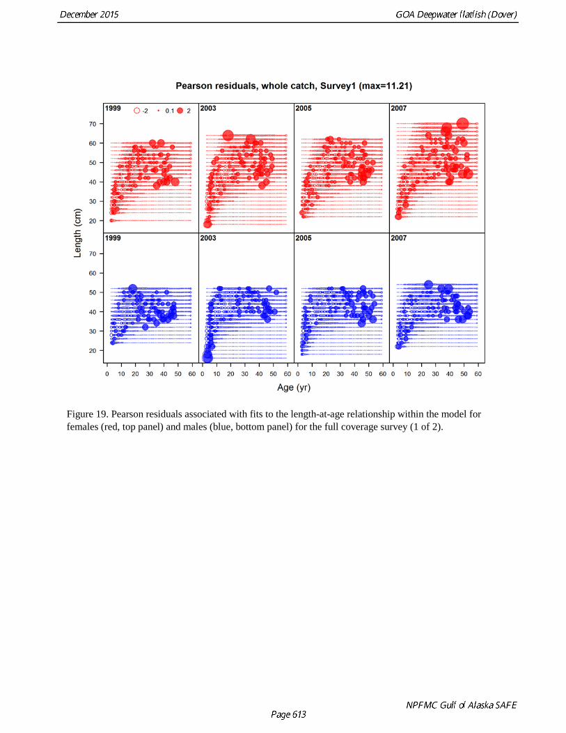
Figure 19. Pearson residuals associated with fits to the length-at-age relationship within the model for females (red, top panel) and males (blue, bottom panel) for the full coverage survey (1 of 2).

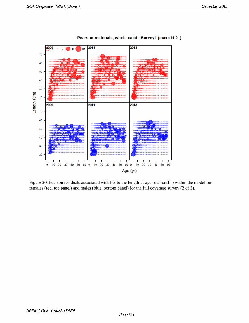
Figure 20. Pearson residuals associated with fits to the length-at-age relationship within the model for females (red, top panel) and males (blue, bottom panel) for the full coverage survey (2 of 2).

Figure 21. Pearson residuals associated with fits to the length-at-age relationship within the model for females (red, top panel) and males (blue, bottom panel) for the shallow coverage survey.

Figure 22. Time series of estimated spawning stock biomass (mt) over time (solid blue line and circles) and asymptotic 95% confidence intervals (blue dashed lines) for the current base case model.

Figure 23. Spawning stock biomass relative to B35% and fishing mortality (F) relative to F35% from 1978-2017 (solid black line), the OFL control rule (dotted red line), the maxABC control rule (solid red line), B35% (vertical grey line), and F35% (horizontal grey line). Projected biomass for 2016 and 2017 are included.

Figure 24. Spawning stock biomass and corresponding 95% asymptotic confidence intervals for base case model runs excluding 0 to 10 years of the most recent data. Each model assumes that recruitment deviations are 0 for years where data are excluded.

Figure 25. Recruitment deviations with corresponding 95% asymptotic confidence intervals (top panel) and age-0 recruits (bottom panel) for base case model runs excluding 0 to 10 years of data. Recruitment deviations are fixed at 0 for years where data are excluded.

Figure 26. The food web from the GOA ecosystem model (Aydin et al., 2007) highlighting Dover sole links to predators (blue boxes and lines) and prey (green boxes and lines). Box size reflects relative standing stock biomass.

Figure 27. Diet composition for Dover sole from the GOA ecosystem model (Aydin et al., 2007).

Figure 28. Decomposition of natural mortality for Dover sole from the GOA ecosystem model (Aydin et al., 2007).

Appendix 5A: Non-Commercial Catches of GOA Deepwater Flatfish (mt)

ADF&G Data Sources

Year

Golden King Crab Pot Survey

Large-Mesh Trawl Survey

Prince William Sound Sablefish

Tagging

Sablefish Longline Survey

Scallop Dredge Survey

Small-Mesh Trawl Survey

1998 386.26 1.7 0.4 1999 1278.85 4.5 2000 300.76 3.5 12.09 2001 577.56 5.1 2002 339.65 10.8 1.84 2003 2093.49 20.8 0.2 83.75 2004 3.709 959.56 12.85 0.06 225.97 2005 12.98 1304.72 3.27 511.54 2006 1.854 250.96 4.463 72.11 169.53 2007 870.07 3.8 28.66 2008 176.31 7 2009 1018.12 4.17 2010 2463.475 35.54 137.78 2011 2666.038 6.35 49.14 2012 1990.99 5.88 28.81 2013 1749.6 37.087 10 23.1 2014 940.04 54.9

Year

IPHC Annual

Longline Survey

2011 12 2012 1 2013 40 2014 75

(Continued on next page)

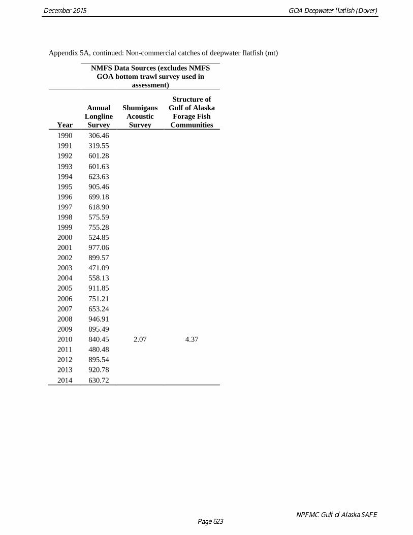
Appendix 5A, continued: Non-commercial catches of deepwater flatfish (mt)

NMFS Data Sources (excludes NMFS GOA bottom trawl survey used in

assessment)

Year

Annual Longline Survey

Shumigans Acoustic Survey

Structure of Gulf of Alaska

Forage Fish Communities

1990 306.46 1991 319.55 1992 601.28 1993 601.63 1994 623.63 1995 905.46 1996 699.18 1997 618.90 1998 575.59 1999 755.28 2000 524.85 2001 977.06 2002 899.57 2003 471.09 2004 558.13 2005 911.85 2006 751.21 2007 653.24 2008 946.91 2009 895.49 2010 840.45 2.07 4.37 2011 480.48 2012 895.54 2013 920.78 2014 630.72

(This page intentionally left blank)