Milestone Report NREL/MP-550-44332 February 2009

Assess the Efficacy of an Aerial Distant Observer Tool Capable of Rapid Analysis of Large Sections of Collector Fields FY 2008 CSP Milestone Report September 2008 G. Jorgensen, F. Burkholder, A. Gray and T. Wendelin

National Renewable Energy Laboratory 1617 Cole Boulevard, Golden, Colorado 80401-3393 303-275-3000 • www.nrel.gov

NREL is a national laboratory of the U.S. Department of Energy Office of Energy Efficiency and Renewable Energy Operated by the Alliance for Sustainable Energy, LLC

Contract No. DE-AC36-08-GO28308

Milestone Report NREL/MP-550-44332 February 2009

Assess the Efficacy of an Aerial Distant Observer Tool Capable of Rapid Analysis of Large Sections of Collector Fields FY 2008 CSP Milestone Report September 2008 G. Jorgensen, F. Burkholder, A. Gray and T. Wendelin

Prepared under Task No. CP0731001

NOTICE

This report was prepared as an account of work sponsored by an agency of the United States government. Neither the United States government nor any agency thereof, nor any of their employees, makes any warranty, express or implied, or assumes any legal liability or responsibility for the accuracy, completeness, or usefulness of any information, apparatus, product, or process disclosed, or represents that its use would not infringe privately owned rights. Reference herein to any specific commercial product, process, or service by trade name, trademark, manufacturer, or otherwise does not necessarily constitute or imply its endorsement, recommendation, or favoring by the United States government or any agency thereof. The views and opinions of authors expressed herein do not necessarily state or reflect those of the United States government or any agency thereof.

Available electronically at http://www.osti.gov/bridge

Available for a processing fee to U.S. Department of Energy and its contractors, in paper, from:

U.S. Department of Energy Office of Scientific and Technical Information P.O. Box 62 Oak Ridge, TN 37831-0062 phone: 865.576.8401 fax: 865.576.5728 email: mailto:reports@adonis.osti.gov

Available for sale to the public, in paper, from: U.S. Department of Commerce National Technical Information Service 5285 Port Royal Road Springfield, VA 22161 phone: 800.553.6847 fax: 703.605.6900 email: orders@ntis.fedworld.gov online ordering: http://www.ntis.gov/ordering.htm

Printed on paper containing at least 50% wastepaper, including 20% postconsumer waste

iii

FY 2008 CSP Milestone Report: Assess the Efficacy of an Aerial Distant Observer Tool

Capable of Rapid Analysis of Large Sections of Collector Fields

Gary Jorgensen, Frank Burkholder, Allison Gray, and Tim Wendelin

September 2008 Executive Summary We performed an assessment of the feasibility of developing an aerial Distant Observer (DO) optical characterization tool. Such a tool is not only viable but offers many benefits to the solar manufacturing industry. The return on R&D investment to develop a DO capability would be significant. For a typical solar power plant, a ±1% optical efficiency improvement or loss is worth about $600,000 in annual revenue. Solar manufacturers very much want a standardized system acceptance test to be developed to more directly address financial exigency. A full-field DO survey could be an important and integral part of such a standard. The aerial DO tool that we have evaluated has features and capabilities that existing tools lack. Direct assessment of tracking errors would be readily provided. Furthermore, the DO would be able to characterize optical misalignments at arbitrary orientations (rather than at 0° elevation only, as required by existing tools) without having to suspend operation. Gravity can cause module facets to sag into a clam shell shape, especially while tracking near 90° elevation. Wind and thermal effects can also result in deformations. The DO allows concentrator modules to be inspected in operational positions that are most representative of in-service performance orientations. Relevant questions were raised regarding the development of a DO capability, along with ways to address associated concerns. The state-of-the-art technologies associated with surveillance platforms, camera systems, and image processing capabilities were evaluated. Three possible operational modes were identified and considered, namely, a large field survey mode (DO-1), analysis of individual modules (DO-2), and infrared (IR) surveys of thermal hotspots in the field (DO-3). We found the following:

• Useful images of absorber tubes that nominally fill trough apertures can be obtained at relatively close distances (< 500 m); such data can provide useful information about optical misalignment.

• Analysis shows that large collector fields (~400 m by 500 m) can be surveyed in less than 4 hours (DO-1 is feasible).

• We have demonstrated that the DO image analysis can be used to predict optical misalignments of a real trough system (DO-2 is feasible).

• Because of resolution limitations associated with infrared cameras, aerial IR imagery capabilities using a tethered blimp platform are probably inadequate (blimp-borne DO-3 is not feasible). An alternative aerial platform may be needed to perform IR characterization in a more timely and cost-effective manner.

iv

Based on our feasibility study, we derived a conceptual design of how to actually go about implementing a DO tool. From a cost perspective, and because of the need to be able to readily redeploy an aerial platform frequently during development, a tethered blimp is the best choice for prototype advancement and proof-of-concept demonstration. Additional hardware specifications and procedures for performing the various characterizations were developed. Prototype deployment of a blimp-borne DO tool during FY 2009 is recommended.

v

Table of Contents

1.0 INTRODUCTION................................................................................................................... 1

2.0 FEASIBILITY STUDY .......................................................................................................... 1

2.1 Potential Benefits and Opportunities .................................................................................... 2

2.2 Operational Modes .................................................................................................................. 3 2.2.1 Qualitative field survey (DO-1) ......................................................................................... 3 2.2.2 Quantitative Module Assessment (DO-2) .......................................................................... 4 2.2.3 IR Measurements (OD-3) .................................................................................................. 9

2.3 State-of-the-Art Technology Capabilities ............................................................................. 9 2.3.1 Assessment of Surveillance Platforms ............................................................................... 9

2.3.1.1 Lighter-Than-Air Platforms ........................................................................................ 9 2.3.1.2 Powered Aircraft ....................................................................................................... 10 2.3.1.3 Commercial Satellites ............................................................................................... 10 2.3.1.4 Aerial Robotic Platforms .......................................................................................... 11

2.3.2 Data Acquisition .............................................................................................................. 14 2.3.2.1 Visible Data Acquisition Issues ................................................................................ 14

2.3.2.1.1 Camera systems and specifications .................................................................... 14 2.3.2.1.1 Storage media and data transmission issues ...................................................... 18

2.3.2.2 Thermally Imaging the Solar Field from a Distance ................................................ 18 2.3.3 Image Analysis................................................................................................................. 20

2.3.3.1 Processing Distant Observer Images ........................................................................ 20

3.0 CONCEPTUAL DESIGN .................................................................................................... 26

3.1 Analysis of Large Field Survey Capabilities (DO-1) ......................................................... 26

3.2 Application of Distant Observer Method to a Real Trough (DO-2) ................................ 29

3.3 Prototype Components and Specifications ......................................................................... 34

4.0 CONCLUSIONS AND RECOMMENDATIONS .............................................................. 34

5.0 ACKNOWLEDGEMENTS ................................................................................................. 35

6.0 REFERENCES ...................................................................................................................... 35

APPENDIX A: OBSERVATION DISTANCE REQUIREMENTS FOR RECEIVER TUBE IMAGE TO FILL TROUGH APERTURE .............................................................................. 39

vi

APPENDIX B: AERIAL IMAGES OF TYPICAL SOLAR TROUGH FIELDS ................. 43

APPENDIX C: TABLES OF CAMERA RESOLUTION PROPERTIES ............................ 45

APPENDIX D: EXAMPLES OF DISTANT OBSERVER IMAGE PROCESSING ........... 52

APPENDIX E: COMPARISON OF COMPUTED RAY TRACE PATTERNS WITH MEASURED IMAGES TO PREDICT OPTICAL MISALIGNMENTS ............................ 57

1

1.0 Introduction The CSP industry has found that optical measurement tools like the Video Scanning Hartmann Optical Tester (VSHOT) and the Theoretical Overlay Photographic (TOP) alignment are invaluable for determining and improving the optical performance of collectors. At present, these instruments are capable of making module-by-module measurements. An aerial borne Distant Observer (DO) method that concurrently views large portions of a collector field in a quick survey mode can provide a rapid assessment of optical misalignments and identify modules in need of closer inspection. This capability would be a useful complementary tool that could designate specific modules in need of subsequent alignment by existing techniques. Such a survey (DO-1) can be performed while a collector field is in operation, thereby minimizing system downtime. A variety of physical effects such as wind damage, mirror change-out, earthquakes, and thermal cycling can cause optical misalignments in the field. An acquired and archived video record would allow detailed off-line analysis, either by visual inspection or automated image processing. Once problem areas have been found, they can be selectively revisited so that more quantitative analyses can be performed (by TOP or DO-2). A refined Distant Observer inspection could supplement existing tools by identifying individual collector and/or receiver misalignment problems, mirror slope error concerns, and tracking errors for in-use concentrator orientations. Module-to-module misalignments can be discerned and an effective full-field intercept factor can be derived. Inspections can be carried out in both the visible spectrum to reveal optical problems and in the infrared to characterize thermal losses. 2.0 Feasibility Study During FY 2008, the objective of this task was to identify an approach to using a Distant Observer method to evaluate the optical accuracy of parabolic trough systems in the field. Our approach was to perform a feasibility study and conceptual design of such a tool and to identify potential concerns such as tracking issues, module-to-module twist problems, and how to identify and separate receiver versus concentrator optical misalignment. Ideally, a prescription for correction of misalignment errors would also be included. The theory behind the Distant Observer method for testing the geometric accuracy of large solar trough collector fields has been outlined by Wood [1]. Wood also discusses various testing configurations and analysis techniques. The state of the art in terms of the ability to attain appropriate viewing positions, data acquisition, and image analysis has dramatically improved in recent years. During FY 2008, we carried out a scoping study (documented herein) to better define what can be learned from Distant Observer techniques. Various means of observing from a distance were assessed, such as by blimp, surveillance robot, remote-controlled helicopter or airplane, airplane fly-by, full-sized helicopter hover pattern, satellite, and others. Different types of aerial telemetry were considered, including viewing the collector field with video and IR cameras. We determined whether adequate resolution can be achieved, the potential for referencing field locations to view positions using global positioning system (GPS) coordinates, and how amenable acquired data is to analysis by the human eye or by digital image processing.

2

2.1 Potential Benefits and Opportunities In the past, industry and laboratory personnel have attempted to use various versions of DO techniques to assess the alignment quality of concentrator modules. To capitalize on their experiences, we contacted those individuals to learn about the benefits and drawbacks that they found. The intent was to identify potential opportunities, along with problems and how they might be addressed and overcome. Questions and related discussions that explore some of these issues are provided below. What is the cost/benefit of developing an aerial DO tool? Several members of the concentrating solar power (CSP) industry have expressed interest in full-field measurements that could provide estimates of an effective full-field intercept factor and detect module-to-module misalignments. At a more fundamental level, solar manufacturers very much want a standardized system acceptance test to be developed. A full-field DO survey could be an integral part of such a standard. If the technical feasibility of a DO tool could be demonstrated and a prototype successfully developed, the return on R&D investment would be significant and provide a large potential benefit for industry. Based on a SAM model of a 100-MW plant with 6 hours of thermal storage, a ±1% optical efficiency improvement or loss is worth about $600,000 in annual revenue. Industry would like to know if optical alignment or performance problems exist and where they occur so that they can be fixed and thereby increase their income and profit. The DO-1 large field survey would rapidly uncover misalignment problems if they exist and identify specific locations of modules that need adjustment. Such a time savings directly translates into additional cost savings. How does the aerial DO approach differ from existing optical alignment tools? The VSHOT provides detailed characterization of the surface figure of concentrator modules but does not differentiate optical misalignments relative to the receiver. Researchers at Sandia National Laboratories found the DO method to be difficult and not feasible for what they were trying to accomplish [2,3], namely, to translate measurements directly into specifications for mirror mounting adjustment (as provided by the TOP alignment instrument). For DO-1, qualitative data that specify where problems exist would be a tremendous asset, so that TOP alignment could know exactly where to emphasize its work. The aerial DO is intended as a complementary rather than a competitive tool. The objective is not to duplicate the TOP alignment optical efficiency test but to determine any other opportunities that could benefit the CSP industry. Are there other advantages to an aerial DO technique relative to existing tools? The use of an aerial platform is particularly suitable for commercial trough power plants because the spacing between rows is so close. A DO approach using aerial platforms would also be advantageous because the platforms can operate and observe troughs at positions other than horizontal, that is, closer to in-use positions. In addition, optical characterization can be carried out during actual operational conditions; there is no need to take rows of troughs off line. What have been the results of previous attempts to implement aerial DO techniques? Florida Power and Light (FPL) has performed aerial video imagery of its CSP plants in the past, and using this information to characterize the optical performance of the field has been difficult.

3

However, in discussions with FPL regarding its aerial images, the company stated that its intent was to use the video images for internal purposes rather than to perform or verify a DO method. What are the operational constraints in terms of observational distance and viewing angle tolerances? From an image resolution perspective, the key to maximizing the amount of useful information that can be processed (“signal”) is to observe at a distance. This is the distance at which the trough aperture would be completely filled if no misalignments were present, and it can be considerably less than 500 m. For example, as shown in Appendix A, the image of a perfectly aligned receiver tube will completely fill the trough aperture at an observation point located approximately182 m away for an LS-2 type of system. When a collector is off-axis with respect to the camera view angle, the images collected will not show the receiver tube, making it difficult to do any type of characterization. However, as a trough rotates through its axis with respect to the camera position, useful optical information can be obtained and analyzed. As discussed in Section 2.2.2, images acquired when a camera system is not aligned perfectly with the optical axis of the concentrator being characterized will appear to be a tracking error, which can be resolved by comparison with other trough rows in the field. What is the likelihood of success in developing an aerial DO technique? The details of an approach that shows how a trough field quad can be surveyed in less than 4 hours is presented in Section 3.1 of this report. As a preproof of concept, we have demonstrated the technique for a single trough facet over a weekend time frame using a $150 6-megapixel (MP) digital camera, a pole mount, and a ray-trace code. This analysis is documented in Section 3.2 of this report. 2.2 Operational Modes 2.2.1 Qualitative Field Survey (DO-1) An initial survey of a collector field will provide a qualitative identification of the mirrors, receivers, and modules that are not properly aligned; we refer to this mode of operation as DO-1. This is a fairly rapid process, requiring less than half a day to survey a subfield having dimensions of ~500 m by 400 m. This process will provide a quick estimate of a full-field intercept factor in terms of the percentage of trough aperture area filled by images of the various receiver elements. In addition, it serves as a complementary technique to existing optical characterization tools. For example, if the TOP alignment tool could survey a trough field in 30 days, and only 10% of the field needs improved alignment, DO-1 could quickly identify the 10% needing alignment and the TOP tool could complete its alignment mission in only 3 days.

4

2.2.2 Quantitative Module Assessment (DO-2) A second, more detailed method, known as DO-2, can be used to perform a quantitative assessment by a more detailed analysis of specified malfunctioning facets. This analysis will allow us to study such concerns as tracking issues (which existing tools cannot discern), module-to-module twist problems, and how to identify and separate receiver versus concentrator optical misalignment. Ideally, this will also generate a prescription for correction of misalignment errors. In addition, concentrator modules can be inspected in operational positions (rather than during suspended service at 0° elevation) that are more representative of in-service performance orientations. To facilitate an evaluation of the DO-2 mode, we used a commercial ray-tracing code (ASAP) to trace rays from the absorber tube to a point of observance for various misaligned geometrical collector configurations. This provides improved maps of what the expected images would look like given the assumed misalignments. Figure 1 shows an isometric view of the calculated aperture patterns for a solar collector assembly (SCA) composed of six LS-2 modules having no optical surface errors. The observation point is at a distance far enough away to ensure that the receiver tube completely fills the trough aperture when no misalignments are present (see Appendix A). The blue color denotes the trough surface, and red represents the image of the receiver tube projected onto the trough. In this case, optical misalignments caused by displacement of the relative trough-to-receiver tube distance (in units of absorber tube diameters) are shown for the SCA modules from left to right having displacements along the optical (z) axis of +2 to -3 absorber tube diameters (Dtube). That is, for the far-left figure, the absorber tube is displaced +2 absorber tube diameters away from the trough; in the far-right module of the SCA, the absorber tube is displaced three absorber tube diameters closer to the trough. The different vertical rows show how the image changes as the trough rotates about the y-axis by an angle ∠y-rot = ±2° through the 0° (on-axis) position. With no misalignment (∆z/Dtube = 0), the trough aperture is completely filled for ∠y-rot = 0°, as expected. When the trough assembly is oriented on-axis (∠y-rot = 0°), roughly the same image will be seen whether the receiver is displaced +2 Dtube or -2 Dtube along the z-axis; the specific misalignment that is occurring is indeterminate. However, observation of the trough through a small angular extent, as it naturally moves during normal tracking operation, allows the uncertainty to be resolved by comparing the sequence of patterns for ∠y-rot = -2° through +2° for ∆z/Dtube = +2 with ∠y-rot = -2° through +2° for ∆z/Dtube = -2. Operationally, this emphasizes the utility of observing the trough as it rotates about its (y) axis through a small angular extent. This also obviates the need to be directly on the optical (z) axis; at worst, being off the true z-axis by a small amount will appear as a tracking error that can be resolved by comparing inter-row timing discrepancies with calculated positions for each row. Thus, if the sequence of images indicates that we are observing “on-axis” for the preponderance of rows observed, then those showing discrepancies can be attributed to tracking errors.

5

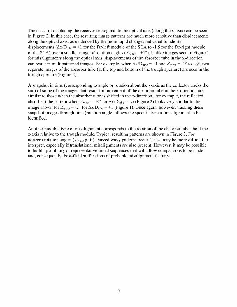
The effect of displacing the receiver orthogonal to the optical axis (along the x-axis) can be seen in Figure 2. In this case, the resulting image patterns are much more sensitive than displacements along the optical axis, as evidenced by the more rapid changes indicated for shorter displacements (∆x/Dtube = +1 for the far-left module of the SCA to -1.5 for the far-right module of the SCA) over a smaller range of rotation angles (∠y-rot = ±1°). Unlike images seen in Figure 1 for misalignments along the optical axis, displacements of the absorber tube in the x-direction can result in multipatterned images. For example, when ∆x/Dtube = +1 and ∠y-rot = -1° to -½°, two separate images of the absorber tube (at the top and bottom of the trough aperture) are seen in the trough aperture (Figure 2). A snapshot in time (corresponding to angle or rotation about the y-axis as the collector tracks the sun) of some of the images that result for movement of the absorber tube in the x-direction are similar to those when the absorber tube is shifted in the z-direction. For example, the reflected absorber tube pattern when ∠y-rot = -¼° for ∆x/Dtube = -½ (Figure 2) looks very similar to the image shown for ∠y-rot = -2° for ∆z/Dtube = +1 (Figure 1). Once again, however, tracking these snapshot images through time (rotation angle) allows the specific type of misalignment to be identified. Another possible type of misalignment corresponds to the rotation of the absorber tube about the z-axis relative to the trough module. Typical resulting patterns are shown in Figure 3. For nonzero rotation angles (∠z-rot ≠ 0°), curved/wavy patterns occur. These may be more difficult to interpret, especially if translational misalignments are also present. However, it may be possible to build up a library of representative timed sequences that will allow comparisons to be made and, consequently, best-fit identifications of probable misalignment features.

6

Figure 1. Images of absorber tube displaced in z-direction superimposed on trough surface as collector rotates through acceptance angle. For each module, the x-axis is up, the y-axis is to the left, and the z (optical) axis is out of the page, as shown.

7

Figure 2. Images of absorber tube displaced in x-direction superimposed on trough surface as collector rotates through acceptance angle. For each module, the x-axis is up, the y-axis is to the left, and the z (optical) axis is out of the page, as shown.

8

Figure 3. Images of absorber tube rotated about z-axis superimposed on trough surface as collector rotates through acceptance angle. For each module, the x-axis is up, the y-axis is to the left, and the z (optical) axis is out of the page, as shown.

9

2.2.3 IR Measurements (DO-3) Another potential application of aerial-borne Distant Observer platforms is the ability to do large field assessments of heat losses from receivers and other components within the heat transfer fluid distribution system. In this case, an infrared imaging system would be incorporated into the platform. Currently, a ground-based IR survey system has been developed and transferred to industry that utilizes GPS navigation to identify heat collection elements (HCEs) and measure their temperatures [4]. One or two field personnel can survey a 30-MW plant in 2 to 3 days with this system. An aerial platform could potentially accomplish this in less than a day, in addition to evaluating other components within the heat transfer fluid loop all the way to the power block. The main technical issue that needs to be addressed is the limited resolution of current IR imaging systems. This limitation will affect how many rows of HCEs can be thermally evaluated at one time and how they are identified and entered into a database. However, this approach has merit for significantly improving the survey time and identifying other field losses that affect both field performance and the safety of personnel.

2.3 State-of-the-Art Technology Capabilities Here we review the state-of-the-art capabilities in surveillance platforms, data acquisition, and image analysis. Data acquisition hardware includes both visible and infrared. 2.3.1 Assessment of Surveillance Platforms Table 1 summarizes the advantages and disadvantages associated with a variety of possible remote/aerial surveillance platforms that can be considered for DO purposes. The various options are discussed below. Based on cost and the need to be able to redeploy an aerial platform frequently during development (because all possibilities and needs cannot be anticipated a priori), we conclude that a blimp is the best choice for prototype advancement and proof-of-concept demonstration. 2.3.1.1 Lighter-Than-Air Platforms Balsley et al. claim that blimps and kites have an advantage over high-velocity aircraft, because “high-spatial resolution measurements are considerably easier to make if the platform is fixed in a ground-based reference” [5]. Blimps also have relatively lower levels of vibrations when compared with those of airplanes and helicopters [6]. Remote-controlled (RC) blimps are not practical or reliable [7]. Small model motorized balloon systems have been made to work indoors [8-14], but no blimp system has been demonstrated to work robustly outdoors (including military blimps). RC airplanes and helicopters are extremely difficult to use and require trained, expert pilots. At least two people are needed to operate such aircraft: a skilled pilot to control the aircraft and another individual to monitor and specify flight details for data acquisition. RC helicopters typically are powered by gas engines, which are difficult to maintain and can crash if they run out of gas or develop engine problems in flight. In contrast, a tethered balloon system can be operated by a single person, is less expensive than an RC helicopter, and is easier to size in terms of lift and payload. Blimps can be stowed in a small trailer and moved from site to site

10

without deflating. They require little maintenance, small holes that may develop are simple to patch, and flaws in flight do not result in catastrophic or damaging crashes (the blimp will slowly descend and can easily be reeled in by hand or with a winch). A blimp can provide a long-duration, low-cost aerial surveillance platform; it can hover over one place and view a large expanse. Typically, blimps have a slower pan rate than planes and a longer operating time than helicopters. They are less expensive and have longer flying times than RC helicopters [15]. A potential drawback with blimp- and kite-borne systems, however, is the need to obtain permission from the Federal Aviation Administration (FAA) to fly a few hundred meters over the ground [5]. According to [16], no person may operate a moored balloon or kite

(1) Less than 152.4 m (500 ft) from the base of any cloud; (2) More than 152.4 m (500 ft) above the surface of the earth; (3) From an area where the ground visibility is less than three miles; or (4) Within five miles of the boundary of any airport.

If needed, a NOTAM (NOTice to AirMen) can be obtained from the FAA. For areas that are restricted by the military, its decisions take precedence over the FAA Code of Federal Regulations (CFR) guidelines. For example, for the Solar Electric Generating System (SEGS) plants located near Edwards Air Force Base in California, we would need to consult with the Operations Group Commander at Edwards. If permission were granted, we would not have to deal with nearby commercial airports (such as Boron or Victorville Airport) to inform them of our presence, because Edwards would do so [17]. 2.3.1.2 Powered Aircraft Helicopters or fixed-wing aircraft are relatively too expensive and can be dangerous (in terms of crash potential). Charter aircraft are very expensive and risky, in terms of having to redo measurements and pay the same fees again if prior data acquisition has to be repeated. Using charter aircraft can also be extremely time-consuming to arrange and properly exploit. Balloon (blimp) photography, in contrast, is the most efficient means of getting a photograph from ground level to 500 feet. A balloon takes some time and effort to set up, but the cost for 1-2 hours of operation is between $250 and $500 [18]. 2.3.1.3 Commercial Satellites Another possibility would be the use of commercial satellites for aerial images. Concerns include the frequency and ability to specify requests for such data and observations. Typically, a single snapshot over a designated wide area of interest (AOI) is provided. For DO analysis, a series of snapshots would be required over a short time period. Until recently, the resolution available from commercial satellites has been ~1 m, as shown in Figure 4 [19, 20]. In September 2008, the GeoEye-1 Satellite Sensor was launched; it has a resolution of 0.41 m [21], which is not adequate for DO analysis. The cost in 2001 for a black and white snapshot with 1-m resolution was $700 for an AOI in the United States and $2500 for an AOI outside the United States [22].

11

Figure 4. Ground sample distances for some civil Earth surface imagers [19]

To achieve smaller ground sample distances (GSD) or increased resolution with satellites, larger focal length optics are needed. The focal length of a lens is given by [19] fl = (working distance * image size) / (object size + image size) . (1) For a satellite in orbit at a working distance of 600 km and an image size equal to the state-of-the-art pixel size of 7 µ, a 1-m object size (GSD) requires a lens with fl = 4.2 m. Achieving a GSD of 0.1 m would require a lens with a focal length 10 times larger, which is not commercially achievable at the present time. Focal length and the size of the focal plane (which depends on the detector system size) are limited by payload volume and mass constraints of commercial satellites. The pointing stability is believed to be too low for small satellites. High-resolution imaging systems generate large amounts of data that need to be stored and transmitted using high-performance equipment. The size, mass, and power use and requirements of such equipment increase with increasing data volumes and rates. The smaller the satellite, the less energy is available for the transmission of data, resulting in smaller integration time periods, high satellite orbit velocities, and, consequently, greater problems in achieving increased resolution [19]. 2.3.1.4 Aerial Robotic Platforms Hovering robotic platforms are being developed for homeland security and first responder emergency purposes. These could potentially be used for DO applications. A vertical or short take-off and landing (VSTOL) portable sensor platform, or PSP, by Stealth Robotics is an example of such a prospective system. However, at the present time it is too expensive and still in the development stage [23, 24].

12

Table 1. Advantages and Disadvantages of Various Possible DO Aerial Platforms

Aerial

Platform Advantages Disadvantages Cost Reference

Airplane • Established/demonstrated technology • Can adjust image acquisition in real time

because operator is on board and there is no problem with hardware communication

• Quick and easy to scan through acceptance angle of each row

• Easier to investigate tracking issues

• Expensive • Cannot hover • Minimum altitude aircraft can legally fly

over populated areas is 1,000 feet (requires increased resolution)

$300-$840 per hour

Helicopter • Can hover • Established/demonstrated technology • Can adjust image acquisition in real time

because operator is on board and there is no problem with hardware communication

• Quick and easy to scan through acceptance angle of each row

• Easier to investigate tracking issues

• Expensive • Minimum altitude aircraft can legally fly

over populated areas is 1,000 feet (requires increased resolution)

Minimum of $500-$600 to arrive on site; once airborne, the rate is $1,200 per hour

[18]

Ultralight Plane

• Quick and easy to scan through acceptance angle of each row

• Easier to investigate tracking issues

• Cannot hover • Difficult to image area of interest for

prolonged period of time • Single operator has to fly & operate data

acquisition equipment

Minimum fees of $120 and about $250 per hour for VSTOL aircraft with removable doors

[18]

RC Airplane • Good control over what and when data are acquired

• Requires trained pilot to fly • Cannot hover • Crash potential can result in damage

13

Aerial Platform

Advantages Disadvantages Cost Reference

RC Helicopter • Can hover • Good control over what and when data

are acquired

• Requires trained pilot to fly • Crash potential can result in damage • Noisy • Large vibrations blur images • Complaints to FAA by public • Relatively low flight time

[26-29]

Blimp • Good control over what and when data are acquired

• If you have a problem, leak is slow and blimp is unlikely to damage collector

• Ideal for heights < 500 ft; can fly up to ~1000 ft

• Without a stabilization feature, observational platform jitter/vibrations could be a problem

~$250/hr [5,16]

Kite • Relatively inexpensive • Can fly at wind speeds greater than a

blimp (>5-8 to 18 m/s)

• Limited payload • Does not have pan/tilt and zoom control

over the camera

Requires much more time on site

[5,30-32]

Satellite • The ultimate Distant Observer • Would observe entire solar field in single

photo

• Poor control over what and when data are acquired (cannot easily obtain desired photographic images on demand)

• Resolution from commercial satellites is limited to ~1 m

• Need series of small time slice photos rather than snapshots

[19,33]

Robot • Hover capability • Programmable control

• Expensive • Not commercially available

[23,24,30,31]

14

2.3.2 Data Acquisition 2.3.2.1 Visible Data Acquisition Issues 2.3.2.1.1 Camera systems and specifications

−= 1

flhRx ε

. To maximize the versatility of the Distant Observer method in terms of applicability to different plant designs, and to maintain a moderately simple operational procedure, plant layouts were evaluated. The layouts of solar trough plants vary in size and orientation, as shown in Appendix B. The average land requirement is 20–25 x 103 m2 (5–6 acres) per megawatt (MW) of installed power, and existing plant sizes are in the range of 14–80 MW. In general, it would be beneficial to characterize as much of the field as possible from a single vantage point. When considering available technology and resources, observing an entire plant from one position may not be feasible. However, using portions of a field may be practical. Having high-resolution images and mapping out potential views of the field are crucial to ensuring that desired portions of a CSP trough field can be imaged. From a data analysis perspective, a resolution of about 10 cm is desired. Multiple cameras are available in the market that could be used for this application. Charge-coupled device (CCD) formats for cameras range from 1–39 MP. Based on the observation distances anticipated and the desired resolution specification, only cameras having a minimum 16-MP CCD format are considered. Illunis, Rollei, and DiMAC offer commercial cameras that qualify; these were evaluated along with compatible matching lenses. To approximate the clarity of the troughs in the field, the resolution of the image at different altitudes was estimated by two different methods. The orientation of the camera with respect to the ground is shown in Figure 5, in which δ is the elevation angle of the camera in degrees, ϕ is the view angle of the lens in degrees, and Rx is the resolution (GSD per pixel) in the x-direction (meter per pixel). The first method is based on rearranging the terms in Eq. 1 above to obtain

, (2)

where

h = height ε = pixel size.

To estimate the length and width of the image view, the resolution is multiplied by the number of pixels, n, as in Eq. 3: xRnL ∗= . (3)

15

For the 16-MP Illunis camera and the 16-, 22-, and 39-MP Rollei cameras, ground-spacing resolution and image view size were calculated using Eqs. 2 and 3. The data at different altitudes are shown in Tables C1–C4 in Appendix C.

Figure 5. Schematic of camera orientation with respect to the ground

One disadvantage to using the first method is that no information is provided regarding image distortion at different altitudes and elevation angles. Image resolution can also be approximated as ( ) ( )[ ]iix hR ϕϕ tantan 1 −∗= + , (4) where the field-of-view angle is defined as ϕα ∗= n . (5) The SEGS III-VII plants are divided into quarter sections called “quads.” A quad was used as the target view area for this feasibility study. A quad is approximately 500 m in the east/west direction and 400 meters in the north/south direction. Figure 6 is a two-dimensional plot of a quad of LS-2 SCAs with 12.5-m spacing.

16

Figure 6. Two-dimensional image of the field orientation for this study

Figure 7 is a plot of pixel camera resolution for an Illunis camera at an altitude of 180 m with a 14 mm Nikon F-mount lens looking straight down at the trough field. The spacing between each line represents the spacing of 100 pixels. Figure 8 is a plot of the same Illunis camera and lens, but the elevation angle of the lens is 20 degrees off the vertical in the counterclockwise direction. The meter-per-pixel resolution is smallest at the center of the image area and gradually increases toward the edges.

Figure 7. Plot of a 16-MP Illunis camera resolution with the camera facing directly down

17

Figure 8. Plot of a 16-MP Illunis camera resolution with the camera facing down and 20º above the

vertical Ground-spacing resolution data for the various Illunis and Rollei cameras deployed at different orientations of interest are presented in Tables C5–C8 in Appendix C. Both the minimum and maximum pixel resolutions are listed in the tables, providing information on the resolution range that is possible over the entire image. The maximum resolutions are greater than the target, but these areas will occur on the outer portions of the images. A pan/tilt gimbal can be used on the aerial platform to provide camera directionality from a single position and ensure that the desired resolution is achieved. The two methods were used to estimate camera resolution, and the results are comparable. The first method provides an average pixel resolution, and the second provides resolution at different angles relative to the lens view angle. An estimate for the camera resolution and distortion is desired to assess the feasibility of the DO concept, and the second method estimates this. In summary, 16-MP cameras at altitudes up to 250 m can provide images resolutions of 0.10 m/pixel at the image center. As shown in Appendix A, if the collector and receiver tube are in their ideal locations, an altitude of 180 m is needed to completely fill the aperture and a 16-MP camera will be sufficient. If higher altitudes are needed, than the meters-per-pixel resolution with a 16-MP camera will increase, reaching up to 0.2 m/pixels at 500 m for a lens with the same focal length. At higher altitudes, a higher megapixel camera would be needed, such as a 39-MP one. With a Rollei 39-MP camera, a resolution of 0.11 m/pixel could be obtained. As long as the aerial platform contains a gimbal to appropriately direct the camera, large portions of a trough field can potentially be evaluated from a single location.

18

2.3.2.1.2 Storage media and data transmission issues

Wireless communications can be beneficial in that it eliminates wire management from the ground up to the aerial platform. This method would require batteries, but they can be placed on the platform and stay with the equipment. It is important that the transceiver be capable of sending large amounts of information in addition to having long-range capabilities. Receivers and transmitters that have these types of capabilities are commercially available (see, for example,

. The imaging and controller information can be transmitted in two different ways—either by a hard line or wireless. A hard line or lines can be used for powering the airborne equipment and for controlling and receiving the data. Wireless transmission cannot be used for powering any of the equipment; it can be used only to send and transmit data. Powering a wireless system could be done by using batteries, but this increases the payload requirements for the aerial platform.

www.omega.com, www.renasis.com, www.advance-security-products.com/). It is also possible to implement a hard line to power and send data back and forth to the platform. One benefit to using a physical line is the elimination of the battery and its payload requirements. The aerial platform could remain in the air for longer periods of time, resulting in more data collection per launch. One concern with powering the platform this way is the weight of the power cable, which could add 23–45 kg (50–100 lb) to the system, depending on the desired altitude. A large variety of aerial platforms are available that have different levels of lift capacity that could address this concern. An additional potential benefit of using hard wire lines is that data can be transmitted over a hard line and wireless communications would no longer be needed.

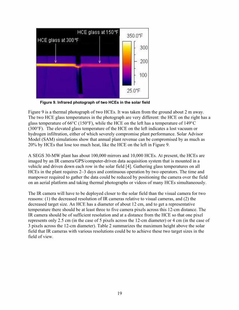
2.3.2.2 Thermally Imaging the Solar Field from a Distance While an optical camera at a distance can investigate the optical performance of large portions of the solar field, an infrared camera can similarly investigate thermal performance. One of the most critical thermal components in the solar field is the receiver, or HCE. The HCE has a glass envelope that transmits visual light and the IR portion of the solar spectrum, but it is opaque to longer IR wavelengths. Consequently, an infrared camera can find the glass temperatures of HCEs, as shown in Figure 9.

19

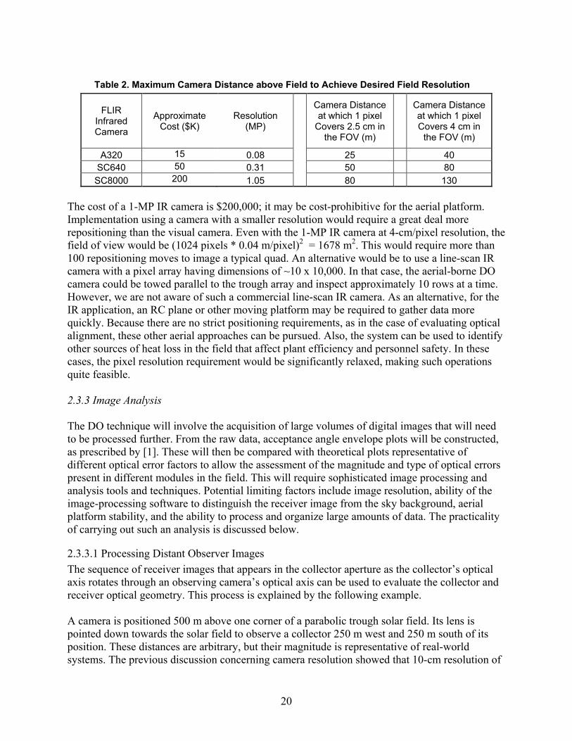
Figure 9 is a thermal photograph of two HCEs. It was taken from the ground about 2 m away. The two HCE glass temperatures in the photograph are very different: the HCE on the right has a glass temperature of 66°C (150°F), while the HCE on the left has a temperature of 149°C (300°F). The elevated glass temperature of the HCE on the left indicates a lost vacuum or hydrogen infiltration, either of which severely compromise plant performance. Solar Advisor Model (SAM) simulations show that annual plant revenue can be compromised by as much as 20% by HCEs that lose too much heat, like the HCE on the left in Figure 9. A SEGS 30-MW plant has about 100,000 mirrors and 10,000 HCEs. At present, the HCEs are imaged by an IR camera/GPS/computer-driven data acquisition system that is mounted in a vehicle and driven down each row in the solar field [4]. Gathering glass temperatures on all HCEs in the plant requires 2–3 days and continuous operation by two operators. The time and manpower required to gather the data could be reduced by positioning the camera over the field on an aerial platform and taking thermal photographs or videos of many HCEs simultaneously. The IR camera will have to be deployed closer to the solar field than the visual camera for two reasons: (1) the decreased resolution of IR cameras relative to visual cameras, and (2) the decreased target size. An HCE has a diameter of about 12 cm, and to get a representative temperature there should be at least three to five camera pixels across this 12-cm distance. The IR camera should be of sufficient resolution and at a distance from the HCE so that one pixel represents only 2.5 cm (in the case of 5 pixels across the 12-cm diameter) or 4 cm (in the case of 3 pixels across the 12-cm diameter). Table 2 summarizes the maximum height above the solar field that IR cameras with various resolutions could be to achieve these two target sizes in the field of view.

Figure 9. Infrared photograph of two HCEs in the solar field

20

FLIR Infrared Camera

Approximate Cost ($K)

Resolution (MP)

Camera Distance at which 1 pixel

Covers 2.5 cm in the FOV (m)

Camera Distance at which 1 pixel Covers 4 cm in

the FOV (m)

A320 15 0.08 25 40 SC640 50 0.31 50 80 SC8000 200 1.05 80 130

The cost of a 1-MP IR camera is $200,000; it may be cost-prohibitive for the aerial platform. Implementation using a camera with a smaller resolution would require a great deal more repositioning than the visual camera. Even with the 1-MP IR camera at 4-cm/pixel resolution, the field of view would be (1024 pixels * 0.04 m/pixel)2 = 1678 m2. This would require more than 100 repositioning moves to image a typical quad. An alternative would be to use a line-scan IR camera with a pixel array having dimensions of ~10 x 10,000. In that case, the aerial-borne DO camera could be towed parallel to the trough array and inspect approximately 10 rows at a time. However, we are not aware of such a commercial line-scan IR camera. As an alternative, for the IR application, an RC plane or other moving platform may be required to gather data more quickly. Because there are no strict positioning requirements, as in the case of evaluating optical alignment, these other aerial approaches can be pursued. Also, the system can be used to identify other sources of heat loss in the field that affect plant efficiency and personnel safety. In these cases, the pixel resolution requirement would be significantly relaxed, making such operations quite feasible. 2.3.3 Image Analysis The DO technique will involve the acquisition of large volumes of digital images that will need to be processed further. From the raw data, acceptance angle envelope plots will be constructed, as prescribed by [1]. These will then be compared with theoretical plots representative of different optical error factors to allow the assessment of the magnitude and type of optical errors present in different modules in the field. This will require sophisticated image processing and analysis tools and techniques. Potential limiting factors include image resolution, ability of the image-processing software to distinguish the receiver image from the sky background, aerial platform stability, and the ability to process and organize large amounts of data. The practicality of carrying out such an analysis is discussed below.

2.3.3.1 Processing Distant Observer Images The sequence of receiver images that appears in the collector aperture as the collector’s optical axis rotates through an observing camera’s optical axis can be used to evaluate the collector and receiver optical geometry. This process is explained by the following example. A camera is positioned 500 m above one corner of a parabolic trough solar field. Its lens is pointed down towards the solar field to observe a collector 250 m west and 250 m south of its position. These distances are arbitrary, but their magnitude is representative of real-world systems. The previous discussion concerning camera resolution showed that 10-cm resolution of

Table 2. Maximum Camera Distance above Field to Achieve Desired Field Resolution

21

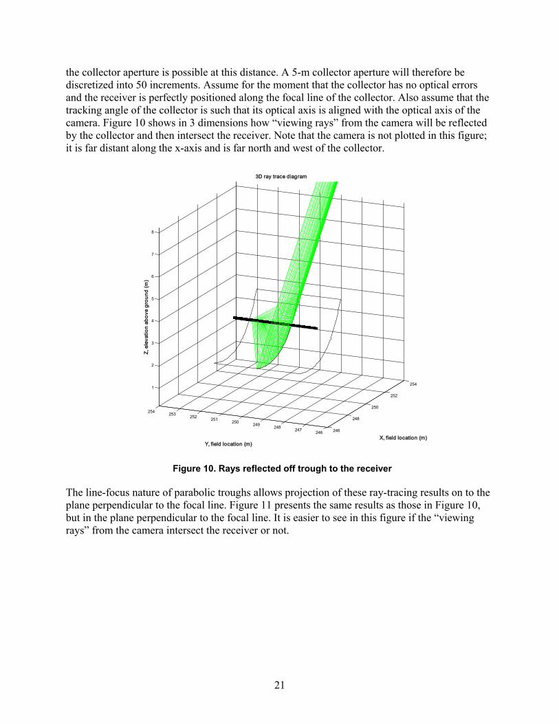
the collector aperture is possible at this distance. A 5-m collector aperture will therefore be discretized into 50 increments. Assume for the moment that the collector has no optical errors and the receiver is perfectly positioned along the focal line of the collector. Also assume that the tracking angle of the collector is such that its optical axis is aligned with the optical axis of the camera. Figure 10 shows in 3 dimensions how “viewing rays” from the camera will be reflected by the collector and then intersect the receiver. Note that the camera is not plotted in this figure; it is far distant along the x-axis and is far north and west of the collector.

246

248

250

252

254

246247248249250251252253254

1

2

3

4

5

6

7

8

X, field location (m)

3D ray trace diagram

Y, field location (m)

Z, e

leva

tion

abov

e gr

ound

(m)

The line-focus nature of parabolic troughs allows projection of these ray-tracing results on to the plane perpendicular to the focal line. Figure 11 presents the same results as those in Figure 10, but in the plane perpendicular to the focal line. It is easier to see in this figure if the “viewing rays” from the camera intersect the receiver or not.

Figure 10. Rays reflected off trough to the receiver

22

246 247 248 249 250 251 252 2530

1

2

3

4

5

6

7

X, field location (m)

Z, e

leva

tion

abov

e gr

ound

(m)

2D ray trace diagram

Figure 11 shows that the 50 “viewing rays” from the camera pointed at this aperture will all reflect off the collector and then intersect with the receiver. Therefore, a photograph taken by the camera of this collector at this tracking angle would show an entirely dark collector aperture—dark because the image of the receiver is dark. As time passes, the collector will continue to track the sun and rotate about its tracking axis from east to west. The camera is stationary. Figure 12 shows how “viewing rays” from the camera reflect off the collector when the collector has rotated 1° (17 milliradians [mrad]) from its position of perfect alignment with the optical axis of the camera.

Figure 11. Perfect alignment of collector and camera optical axes, with 0° (0 mrad) difference between axes

23

246 247 248 249 250 251 252 253

1

2

3

4

5

6

7

8

X, field location (m)

Z, e

leva

tion

abov

e gr

ound

(m)

2D ray trace diagram

The red rays in Figure 12 indicate rays that miss the receiver. When the photograph is taken at this collector angle, only the bottom three-quarters of the collector will appear dark. The upper portion will reflect the sky and therefore appear light on the photograph. Figures 13 and 14 show what happens as the collector continues to rotate, increasing the difference between the collector optical axis and the camera optical axis. A photograph of the aperture in 13 would show a dark region near its center but light edges, and a photograph of the aperture in 14 would be entirely light, showing only the sky.

Figure 12. -17 mrad difference between collector and camera optical axes

24

246 247 248 249 250 251 252 253

1

2

3

4

5

6

7

8

X, field location (m)

Z, e

leva

tion

abov

e gr

ound

(m)

2D ray trace diagram

246 247 248 249 250 251 252 253

1

2

3

4

5

6

7

8

X, field location (m)

Z, e

leva

tion

abov

e gr

ound

(m)

2D ray trace diagram

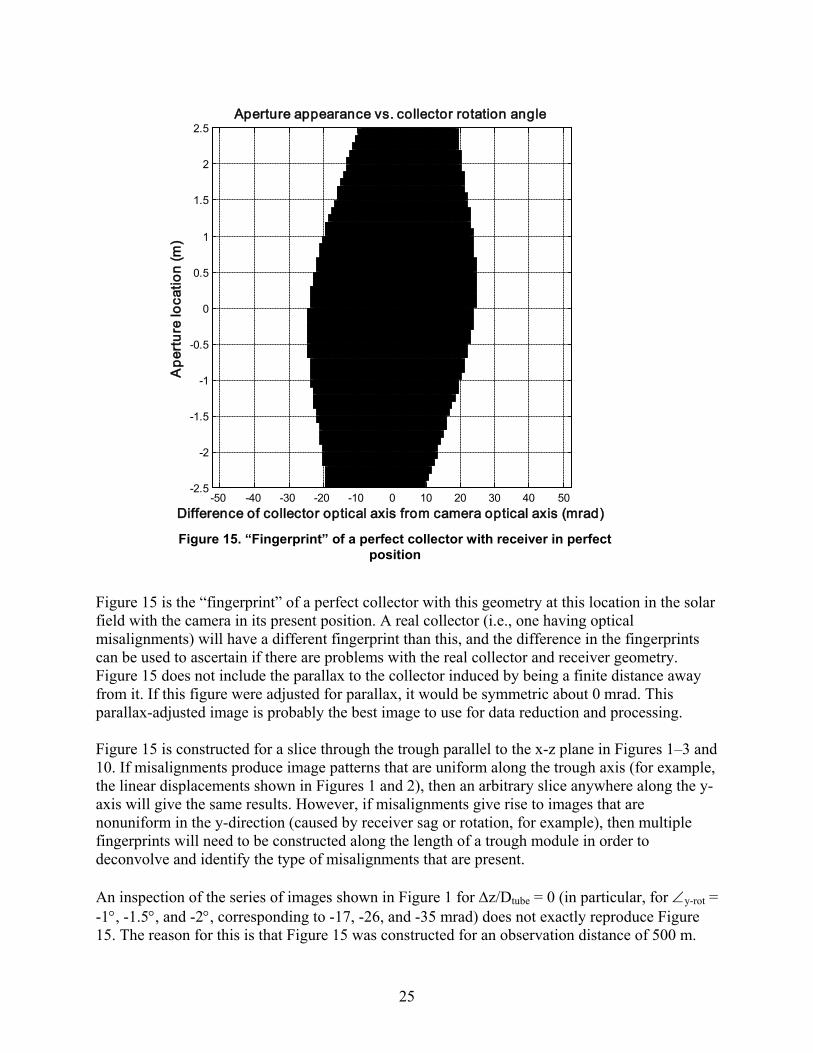
The purpose of taking photographs of the collector as its optical axis rotates through the optical axis of the camera is to create the plot shown in Figure 15. This plot summarizes the receiver image coverage information in the trough aperture presented in Figures 11–14, as well as receiver image coverage information for many other collector rotation angles relative to the camera axis. The results of the ray-trace plot with perfect alignment, Figure 11, are plotted at 0 mrad on the x-axis of Figure 15. The continuous vertical black line above 0 mrad shows that all aperture locations appear black at the 0 mrad difference between the collector and optical axes. The results from Figures 12, 13, and 14 occur at -17, -26, and -35 mrad, respectively. At -35 mrad, no part of the receiver reflected in the collector is visible from the camera, so in Figure 15 the column above -35 mrad is completely white.

Figure 13. -26 mrad difference between axes Figure 14. -35 mrad difference between axes

25

-50 -40 -30 -20 -10 0 10 20 30 40 50-2.5

-2

-1.5

-1

-0.5

0

0.5

1

1.5

2

2.5

Difference of collector optical axis from camera optical axis (mrad)

Ape

rtur

e lo

catio

n (m

)

Aperture appearance vs. collector rotation angle

Figure 15 is the “fingerprint” of a perfect collector with this geometry at this location in the solar field with the camera in its present position. A real collector (i.e., one having optical misalignments) will have a different fingerprint than this, and the difference in the fingerprints can be used to ascertain if there are problems with the real collector and receiver geometry. Figure 15 does not include the parallax to the collector induced by being a finite distance away from it. If this figure were adjusted for parallax, it would be symmetric about 0 mrad. This parallax-adjusted image is probably the best image to use for data reduction and processing. Figure 15 is constructed for a slice through the trough parallel to the x-z plane in Figures 1–3 and 10. If misalignments produce image patterns that are uniform along the trough axis (for example, the linear displacements shown in Figures 1 and 2), then an arbitrary slice anywhere along the y-axis will give the same results. However, if misalignments give rise to images that are nonuniform in the y-direction (caused by receiver sag or rotation, for example), then multiple fingerprints will need to be constructed along the length of a trough module in order to deconvolve and identify the type of misalignments that are present. An inspection of the series of images shown in Figure 1 for ∆z/Dtube = 0 (in particular, for ∠y-rot = -1°, -1.5°, and -2°, corresponding to -17, -26, and -35 mrad) does not exactly reproduce Figure 15. The reason for this is that Figure 15 was constructed for an observation distance of 500 m.

Figure 15. “Fingerprint” of a perfect collector with receiver in perfect position

26

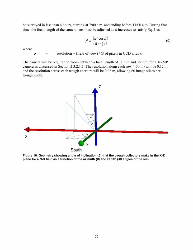
Figure 1 depicts how the trough aperture appears from ~182 m away, the minimum distance at which the image of the receiver tube completely fills the trough aperture for an LS-2 design. Specific examples of the power and utility of this approach are presented in Appendix D. The appendix demonstrates how this methodology can be successfully applied to a variety of optical misalignments. The ability to process images from modules having real-world surface errors is also shown. 3.0 Conceptual Design 3.1 Analysis of Large Field Survey Capabilities (DO-1) In this section, we analyze the time and resolution requirements of performing a large-area (~quad) trough field survey. For a north-south (N-S) field layout (with east-west tracking), the angle of inclination (β) that the trough collectors makes in the X-Z plane is a function of the azimuth (θ) and zenith (φ) angles of the sun. The geometry is shown in Figure 16 and the inclination angle is given by ( ) ( )[ ]θφβ sintantan 1−= . (6) The azimuth (θ) and zenith (φ) angles of the sun can be calculated from the latitude and longitude coordinates of the site (available from GPS), day of the year, and local time [34]. The time at which the image of the receiver completely fills the trough aperture (for perfect alignment) occurs when the camera view angle equals the collector orientation angle:

( )

∆−+

= −

hid 1tan 1β (7)

or

( ) ( ) ( )hid ∆−+

=1sintan θφ , (8)

where, as shown in Figure 17,

∆ = row spacing h = height of the camera i = row index d = distance of camera from the start of the field (i = 1).

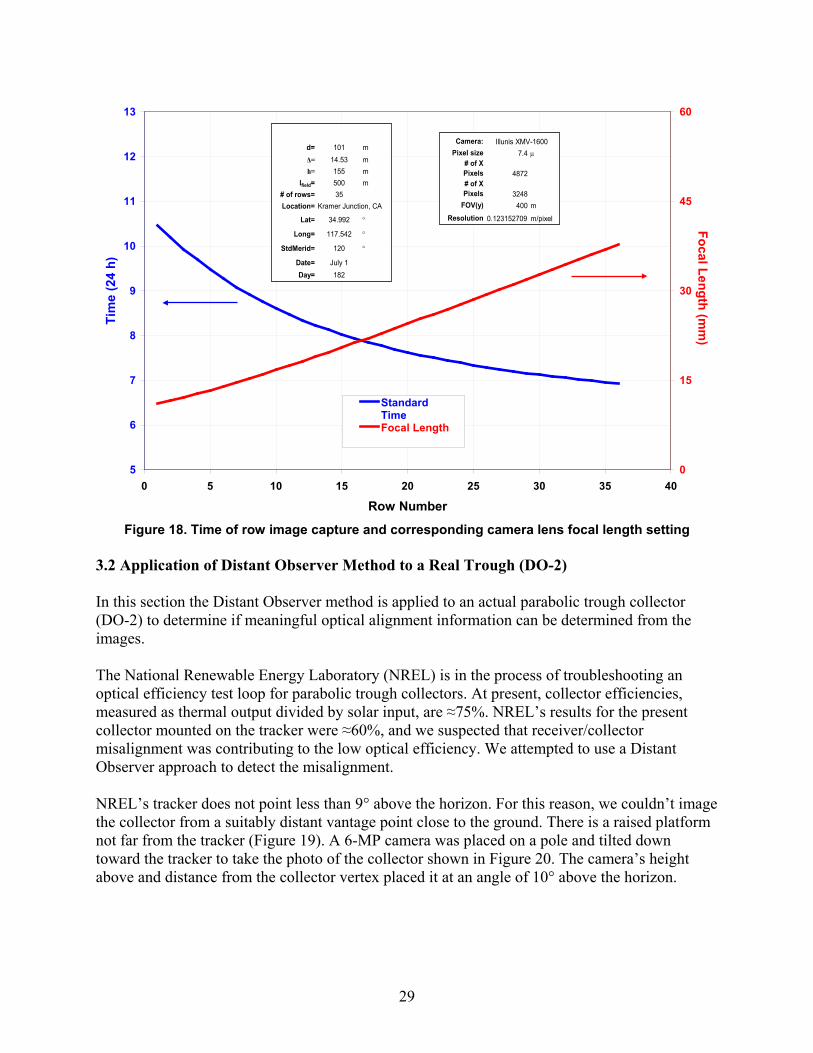
Solving Eq. 8 for time, we can calculate the view angle, β, at which to tilt the camera system to view each of i rows as they are moving through the sun-tracking angle at which the absorber tube completely fills the trough aperture for ideally aligned concentrators. As an example, for an LS-2 quad, if the blimp is deployed at an altitude of approximately 152 m (to prevent exceeding the 500-ft height ceiling), the distance from the blimp to the first row needs to be d = 101 m so that the distance to each row is at least 182 m to ensure that the image of the absorber tube in each row completely fills the trough aperture. As seen in Figure 18, the complete quad (36 rows) can

27

be surveyed in less than 4 hours, starting at 7:00 a.m. and ending before 11:00 a.m. During that time, the focal length of the camera lens must be adjusted as β increases to satisfy Eq. 1 as

( )( ) 1/

cos/+

=ε

βRhfl (9)

where R = resolution = (field of view) / (# of pixels in CCD array). The camera will be required to zoom between a focal length of 11 mm and 38 mm, for a 16-MP camera as discussed in Section 2.3.2.1.1. The resolution along each row (400 m) will be 0.12 m, and the resolution across each trough aperture will be 0.08 m, allowing 60 image slices per trough width.

Figure 16. Geometry showing angle of inclination (β) that the trough collectors make in the X-Z plane for a N-S field as a function of the azimuth (θ) and zenith (Φ) angles of the sun

28

Figure 17. Geometry for calculation of row image capture timing during field survey

29

5

6

7

8

9

10

11

12

13

0 5 10 15 20 25 30 35 40

Row Number

Tim

e (2

4 h)

0

15

30

45

60Focal Length (m

m)

StandardTimeFocal Length

d= 101 mΔ= 14.53 mh= 155 m

lfield= 500 m# of rows= 35Location=

Lat= 34.992 °

Long= 117.542 °

StdMerid= 120 °

Date= July 1Day= 182

Kramer Junction, CA

Camera:Pixel size 7.4 µ

# of XPixels 4872# of XPixels 3248

FOV(y) 400 mResolution 0.123152709 m/pixel

Illunis XMV-1600

Figure 18. Time of row image capture and corresponding camera lens focal length setting

3.2 Application of Distant Observer Method to a Real Trough (DO-2) In this section the Distant Observer method is applied to an actual parabolic trough collector (DO-2) to determine if meaningful optical alignment information can be determined from the images. The National Renewable Energy Laboratory (NREL) is in the process of troubleshooting an optical efficiency test loop for parabolic trough collectors. At present, collector efficiencies, measured as thermal output divided by solar input, are ≈75%. NREL’s results for the present collector mounted on the tracker were ≈60%, and we suspected that receiver/collector misalignment was contributing to the low optical efficiency. We attempted to use a Distant Observer approach to detect the misalignment. NREL’s tracker does not point less than 9° above the horizon. For this reason, we couldn’t image the collector from a suitably distant vantage point close to the ground. There is a raised platform not far from the tracker (Figure 19). A 6-MP camera was placed on a pole and tilted down toward the tracker to take the photo of the collector shown in Figure 20. The camera’s height above and distance from the collector vertex placed it at an angle of 10° above the horizon.

30

Figure 19. Raised platform from which photos of the collector were taken

Figure 20. Photograph of collector. Collector optical axis 10° above horizon. Camera optical axis 10° above horizon. Collector optical axis – camera optical axis = 0°. Letters and numbers form grid to refer to mirror panels.

31

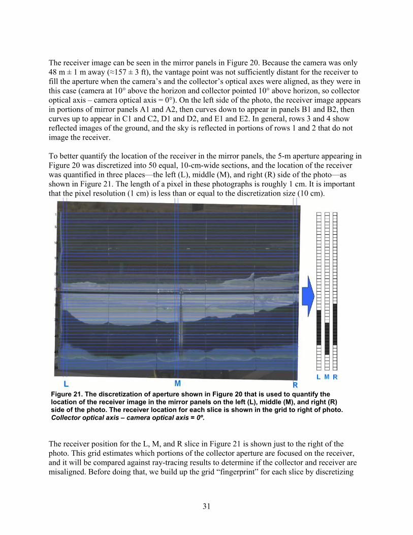
The receiver image can be seen in the mirror panels in Figure 20. Because the camera was only 48 m ± 1 m away (≈157 ± 3 ft), the vantage point was not sufficiently distant for the receiver to fill the aperture when the camera’s and the collector’s optical axes were aligned, as they were in this case (camera at 10° above the horizon and collector pointed 10° above horizon, so collector optical axis – camera optical axis = 0°). On the left side of the photo, the receiver image appears in portions of mirror panels A1 and A2, then curves down to appear in panels B1 and B2, then curves up to appear in C1 and C2, D1 and D2, and E1 and E2. In general, rows 3 and 4 show reflected images of the ground, and the sky is reflected in portions of rows 1 and 2 that do not image the receiver. To better quantify the location of the receiver in the mirror panels, the 5-m aperture appearing in Figure 20 was discretized into 50 equal, 10-cm-wide sections, and the location of the receiver was quantified in three places—the left (L), middle (M), and right (R) side of the photo—as shown in Figure 21. The length of a pixel in these photographs is roughly 1 cm. It is important that the pixel resolution (1 cm) is less than or equal to the discretization size (10 cm).

The receiver position for the L, M, and R slice in Figure 21 is shown just to the right of the photo. This grid estimates which portions of the collector aperture are focused on the receiver, and it will be compared against ray-tracing results to determine if the collector and receiver are misaligned. Before doing that, we build up the grid “fingerprint” for each slice by discretizing

Figure 21. The discretization of aperture shown in Figure 20 that is used to quantify the location of the receiver image in the mirror panels on the left (L), middle (M), and right (R) side of the photo. The receiver location for each slice is shown in the grid to right of photo. Collector optical axis – camera optical axis = 0º.

32

photos taken with the collector at 9°, 11°, 12°, and 13° above the horizon, as shown in Figures 22, 23, 24, and 25, respectively.

As the collector rotates from 9° above the horizon upward, the image of the receiver (as shown in Figures 22, 21, and 23–25) gradually moves off the bottom of the collector. Figure 26 summarizes the motion of the receiver pattern for each slice (L, M, R) as a function of the difference between the collector’s optical axis and the camera’s optical axis.

Figure 22. Collector 9° above horizon. Coll. opt. ax. – cam. opt. ax. = -1°.

Figure 23. Collector 11° above horizon. Coll. opt. ax. – cam. opt. ax. = 1°.

Figure 24. Collector 12° above horizon. Coll. opt. ax. – cam. opt. ax. = 2°.

Figure 25. Collector 13° above horizon. Coll. opt. ax. – cam. opt. ax. = 3°.

33

Figure 26 is the “fingerprint” for each slice on the collector. These fingerprints can be compared to ray-tracing results to determine if and how much the receiver is misaligned to the mirror panels that occur in each slice. This process is carried out in Appendix E. The results indicate that the center of the real receiver is sagging about 7 cm lower than where it should be. The left end of the receiver is 5 cm below the optical axis and 2 cm too far away from the vertex, and the right end is 3 cm below the optical axis and 1 cm too far away from the vertex. Changes were made to the optical efficiency test loop receiver position in response to the ray-trace calculations detailed in Appendix E. The result was a 10% increase in optical efficiency. This increase in performance indicates successful application of the Distant Observer method in this instance. We are planning another series of photographs to document the new geometry, as well as more accurate distance measurement methods to decrease the variability in the receiver position that arises from geometric uncertainty.

Figure 26. Digitized receiver position from photographs of collector for each slice (L, M, R) as the collector’s optical axis rotated through the camera’s optical axis

34

This is a simple example of what may be accomplished using an aerial Distant Observer approach. However, we recognize that more distant vantage points will mean larger amounts of information and, consequently, require more processing. Processing requirements may limit the detail at which this type of analysis is carried out. 3.3 Prototype Components and Specifications The main emphasis of the prototype will be to demonstrate and prove the DO-1 concept. The prototype aerial platform will be a tethered blimp [35]. The number of tether lines can range between 1 and 3, depending on wind speed and direction. Three lines can provide greater stability but may also adversely constrain the location and orientation of the blimp. The tethers can be connected to a winch or reel that can be hand-held and operated during prototype development. For fully operational DO systems, the winch/reel can be interfaced with a golf cart or all-terrain vehicle. Attached to the blimp will be a three-axis gyroscopic stabilized platform to minimize vibrations and jitter. This will interface with a pan/tilt gimbal stage that will hold a digital camera and allow it to be pointed as directed. The camera will nominally have 16-MP resolution to allow rapid (< ½ day) survey of a trough subfield (quad) having dimensions of ~500 m x 400 m. The camera will have an image stabilization capability (probably as a post-processing feature to maintain high real-time resolution) to further reduce the effects of vibrations and optimize the quality of acquired digital photography. A camera capable of GPS and time stamps would expedite the observing program protocol. For a given local time, the trough row to be inspected is identified. GPS data then specify the angle β at which to point the camera. This designates the tilt angle for moving the camera. Time also specifies the focal length for zooming the camera lens. For each row, a series of photos are taken as the trough tracks through its maximum acceptance angle. The acquired photos must then either be stored or transmitted to the ground station. Alternatively, it may be possible to use a precision laser ranging device to accurately determine the distance between the camera and the trough row of interest. Remote access and control will be required of the pan/tilt, camera focus and zoom, and image telemetry. Alternatively, the tether line(s) can be used to provide control commands and/or power from the ground to the aerial system and to allow downloading of digital images. Other features that will need to be considered during prototype development include the use of auto-focus lenses, lens filters to enhance contrast, and the possibility of dual camera payloads (e.g., any combination of digital cameras, analog video cameras, and IR cameras). 4.0 Conclusions and Recommendations We have performed an assessment of the feasibility for development of a DO tool that can characterize optical misalignments of solar trough modules. Relevant questions regarding the development of a DO capability were raised, along with ways to address associated concerns. The state-of-the-art technologies associated with surveillance platforms, camera systems, and image processing capabilities were evaluated. Three possible operational modes were identified and considered, namely, a large field survey mode (DO-1), analysis of individual modules (DO-2), and infrared surveys of thermal hotspots in the field (DO-3). We found the following:

35

• Useful images of absorber tubes that nominally fill trough apertures can be obtained at

relatively close distances (<500 m); such data can provide useful information about optical misalignment.

• Analysis shows that large collector fields (~400 m by 500 m) can be surveyed in less than 4 hours (DO-1 is feasible).

• We have demonstrated that the DO image analysis can be used to predict optical misalignments of a real trough system (DO-2 is feasible).

• Because of resolution limitations associated with infrared cameras, aerial IR imagery capabilities using a tethered blimp platform are probably not adequate (blimp-borne DO-3 is not feasible). An alternative aerial platform may be needed to perform IR characterization in a more timely and cost-effective manner.

Based on our feasibility study, we derived a conceptual design of how to actually go about implementing a DO tool. From a cost perspective, and the need to be able to readily redeploy an aerial platform frequently during development, a tethered blimp is the best choice for prototype advancement and proof-of-concept demonstration. Additional hardware specifications and procedures for performing the various characterizations were developed. Prototype deployment of a blimp-borne DO tool during FY 2009 is recommended. 5.0 Acknowledgements This work was performed under DOE Contract No. DE-AC36-99-GO10337. The authors would like to thank a number of industry reviewers for their useful comments and suggestions, including Nicholas Potrovitza and Marc Newmarker of Acciona Solar Power, Inc.; Randy Gee of SkyFuel, Inc.; and Hank Price of Abengoa Solar, Inc. We would also like to thank Chuck Kutscher and Mark Mehos of NREL for their reviews and numerous productive technical discussions throughout this project. 6.0 References 1. Wood, R. L., Distant Observer Techniques for Verification of Solar Concentrator Optical Geometry, UCRL53220, Lawrence Livermore National Laboratory, Livermore, CA, 1981. 2. Diver, R. B., and Moss, T. A., “Practical Field Alignment of Parabolic Trough Solar Concentrators,” ASME J. Sol. Energy Eng., Vol. 129, 2007, pp. 153-159. 3. Moss, T. A., and Brosseau, D. A., “Test Results of a Schott Trough Receiver Using a LS-2 Collector,” Proceedings of ISES 2005, International Solar Energy Conference, Orlando, FL, August 6-12, 2005. 4. Price, H., Forristall, R., Wendelin, T., Lewandowski, A., Moss, T., and Gummo, C., “Field Survey of Parabolic Trough Receiver Performance,” Proceedings of ISEC: ASME 2006, Denver, Colorado, July 8-13, 2006.

36

5. Balsley, B. B., Jensen, M. L., Frehlich, R. G., Eaton, F. D., Bishop, K. P., and Hugo, R. J., “In-situ turbulence measurement technique using state-of-the-art kite/blimp platforms,” Airborne Laser Advanced Technology II, Steiner, T. D., and Merritt, P. H., Eds., Proceedings of SPIE Vol. 3706, 1999, pp. 2-10. 6. Elfes, A., Bergerman, S., and Ramos, M., “A Semi-Autonomous Robotic Airship for Environmental Monitoring Missions,” Proceedings of the 1998 IEEE International Conference on Robotics and Automation, Vol. 4, 1998, pp. 3449-3455. 7. Liestenfeltz, K., private communication, Floatagraph Technologies, LLC, Silver Spring, MD, 301-563-3082, May 21, 2008. 8. Ogata, T., Matsuda, S., Tan, J.K., and Ishikawa, S., “Real-time Human Motion Recognition by an Aerial Robot,” IEEE International Conference on Systems, Man and Cybernetics, Vol. 6, 2004, pp. 5290-5295. 9. Green, W.E., Sevcik, K.W., and Oh, P.Y., “A Competition to Identify Key Challenges for Unmanned Aerial Robots in Near-Earth Environments,” Proceedings of ICAR '05, the 12th International Conference on Advanced Robotics, 2005, pp. 309-315. 10. Sevcik, K.W., Green, W.E., and Oh, P.Y., “Exploring Search-and-Rescue in Near-Earth Environments for Aerial Robots,” Proceedings of the 2005 IEEE/ASME International Conference on Advanced Intelligent Mechatronics, 2005, pp. 699-704. 11. Ko, J., Klein, D.J., Fox, D., and Haehnel, D., “Gaussian Processes and Reinforcement Learning for Identification and Control of an Autonomous Blimp,” IEEE International Conference on Robotics and Automation, 2007, pp. 742-747. 12. Walkenhorst, B.T., Miner, G.F., and Arnold, D.V., “A Low Cost, Radio Controlled Blimp as a Platform for Remote Sensing,” Proceedings of IGARSS 2000, the IEEE 2000 International Geoscience and Remote Sensing Symposium, Vol. 5, 2000, pp. 2308-2309. 13. Fukao, T., Fujitani, K., and Kanade, T., “An Autonomous Blimp for a Surveillance System,” IROS 2003, Proceedings of the 2003 IEEE/RSJ International Conference on Intelligent Robots and Systems, Vol. 2, 2003, pp. 1820-1825. 14. Fukao, T., Fujitani, K., and Kanade, T., “Image-Based Tracking Control of a Blimp”, Proceedings of the 42nd IEEE Conference on Decision and Control, Vol. 5, 2003, pp. 5414-5419. 15. http://www.galaxyblimps.com/videography.html 16. http://www.dot.ca.gov/hq/planning/aeronaut/htmlfile/part101.php#Sec.%20101.1 (14 CFR; Aeronautics and Space; Chapter I; Federal Aviation Administration, Department of Transportation (Continued); Subchapter F –Air Traffic and General Operating Rules; Part 101 –

37

Moored Balloons, Kites, Unmanned Rockets and Unmanned Free Balloons; §101.13, Operating limitations) 17. Gries, Bill, Private communication, Edwards Air Force Base, Antelope Valley (LA), CA, 661-277-2446, July 14, 2008. 18. http://www.aerialproducts.com/aerial-photography/aerial-photography-equipment.html 19. Sandau, R., “High-resolution imaging with small satellites: what are the possibilities and limitations?” Sensors and Systems for Space Applications, Howard, R. T., and Richards, R. D., Eds., Proceedings of SPIE Vol. 6555, 2007. 20. Doescher, S. W., Ristyb, R., and Sunne, R. H., “Use of Commercial Remote Sensing Data in Support of Emergency Response,” ISPRS Workshop on Service and Application of Spatial Data Infrastructure, XXXVI (4/W6), 2005, pp. 121-124. 21. “GeoEye-1 Satellite Sensor Launched Successfully from Vandenberg Air Force Base in California,” September 6, 2008, http://news.satimagingcorp.com/. 22. “Space Imaging Announces New Commercial Pricing on IKONOS Satellite Imagery Products,” December 13, 2001, http://www.spaceref.com/news/viewpr.html?pid=6911. 23. Johnson, S. A., and Vallely, J. M., “A Portable Aerial Surveillance Robot,” Sensors and Command, Control, Communications, and Intelligence (C3I) Technologies for Homeland Security and Homeland Defense V, Carapezza, E. M., Ed., Proceedings of SPIE, Vol. 6201, 2006. 24. http://stealthrobotics.com/. 25. Hain, J. H. W., “Lighter-than-air Platforms (Blimps and Aerostats) for Oceanographic and Atmospheric Research and Monitoring,” OCEANS 2000 MTS/IEEE Conference and Exhibition, Vol. 3, 2000, pp. 1933-1936. 26. Jones, H. L., Frew, E. W., Woodley, B. R., and Rock, S. M., “Human-robot interaction for field operation of an autonomous helicopter,” Mobile Robots XIII and Intelligent Transportation Systems, Choset, H. M., Gage, D. W., Kachroo, P., Kourjanski, M. A., and de Vries, M. J., Eds., Proceedings of SPIE, Vol. 3525, 1999. 27. Zhao, X., Liu, J., and Tan, M., “A Remote Aerial Robot for Topographic Survey,” IEEE/RSJ International Conference on Intelligent Robots and Systems, 2006, pp. 3143-3148. 28. Gordon, M., Kondor, S., Corban, E., and Schrage, D., “Rotorcraft Aerial Robot-Challenges and Solutions,” 12th DASC., AIAA/IEEE Digital Avionics Systems Conference, 1993, pp. 298-305.

38

29. Onosato, M., Takemura, F., Nonami, K., Kawabata, K., Miura, K., and Nakanishi, H., “Aerial Robots for Quick Information Gathering in USAR,” International Joint Conference of SICE-ICASE, 2006, pp. 3435-3438. 30. Oh, P.Y., and Green, W. E., “ Mechatronic Kite and Camera Rig to Rapidly Acquire, Process and Distribute Aerial Images,” IEEE/ASME Transactions on Mechatronics, December 2004, Vol. 9, No. 4, pp. 671-678. 31. Oh, P.Y., Joyce, M., and Gallagher, J., “Designing an Aerial Robot for Hover-and-Stare Surveillance,” Proceedings of ICAR '05, the 12th International Conference on Advanced Robotics, 2005, pp. 303-308. 32. Murray, J. C., Neal, N. J., and Labrosse, F., “Intelligent Kite Aerial Platform for Site Photography,” IEEE International Conference on Automation Science and Engineering, 2007, pp. 548-553. 33. Nolan, J. R., “Comparison of Commercial High-Resolution Satellite Imagery,” Proceedings of the IEEE Aerospace Conference, Vol. 2, 2001, pp. 2/925-2/930. 34. Duffie, J. A., and Beckman, W. A., Solar Engineering of Thermal Processes, 2nd Ed., John Wiley & Sons, Inc., New York, 1991, pp. 11-16. 35. McKerrow, P. J., and Ratner, D., “The design of a tethered aerial robot,” IEEE International Conference on Robotics and Automation, 2007, pp. 355-360.

39

Appendix A Observation Distance Requirements for Receiver Tube Image to Fill

Trough Aperture Figure A-1 displays the paths of rays starting at a point source location along the optical axis that are traced to a reflecting trough and then to the absorber tube. The reverse ray trace corresponds to the image of the absorber tube projected onto the trough surface as seen from the observation point. If there are no misalignment errors, then the amount of trough aperture filled by the absorber tube image will depend on the distance to the observation point, z = ℓ in Figure A-1. A more detailed diagram of the parameters that control the amount of aperture area filled by the absorber tube image is shown in Figure A-2. At z = ℓ, the extreme edge ray making an angle γ with the optical axis intersects the trough at z = s, is reflected, and just intersects the absorber tube. If the observation point were any closer to the trough, the launch angle γ would be larger and the reflected ray would miss the absorber tube. The distance from the edge of the trough (x = w/2) to the center of the absorber tube is

( ) ( )22 2/wsfb +−= , (A-1) where

f = focal length of parabolic trough s = sag = (w/2)2 / (4f) w = trough aperture.

Then, from Figure A-2,

( )s

wb

Dtube

−==

0

2/2/tan

γ , (A-2)

where Dtube = outer diameter of absorber tube ℓ0 = observation point along the optical (z) axis at which the image of the absorber

tube completely fills the trough aperture. On the surface of the parabolic trough,

f

xz4

2

= , (A-3)

where x = x-coordinate of a point on the trough z = corresponding z-coordinate of a point on the trough.

Using Eq. A-3 in Eq. A-1 to obtain b, we have from Eq. A2,

( ) ( )2/

2/0

tubeDsfws +∗

+= . (A-4)

40

For an LS-2 trough (f = 1.49 m; w = 5 m) and an absorber tube having Dtube = 0.07 m, the result is an observation distance of ℓ0 ≈ 182 m. In general, at some distance z = ℓ, the ratio of filled aperture area will be x / (w/2) and

( )2/tubeDzfxz +

+= . (A-5)

Figure A-3 shows the ray-traced images for an LS-2 module observed at a number of distances z = ℓ. The light blue color is the surface of the trough, and the red color corresponds to the rays that produce the image of the absorber tube in the trough aperture. As expected, the trough aperture is completely filled at a distance ℓ = ℓ0 ≈ 182 m. The trough aperture is half filled at ℓ ≈ 63 m. The fraction of filled aperture as a function of the observation point, as calculated from Eq. A-5, is presented in Figure A-4. By observing at a distance ≈ ℓ0 (which may be considerably less than 500 m), the full aperture area provides usable information and maximizes the spatial resolution capability of acquired images.

Figure A-1. Ray trace of absorber tube image in trough aperture as viewed from observation point

at z = ℓ

41

Figure A-2. Geometry related to the amount of aperture area filled by the absorber tube image as

viewed at an observation point at z = ℓ

Figure A-3. Absorber tube image in LS-2 trough aperture for various observation distances (m)

42

0.0

0.2

0.4

0.6

0.8

1.0

0.0 0.2 0.4 0.6 0.8 1.0

l / l0

x / (

w/2

)

f = 1.49 mw = 5 mD = 0.07 m

sag = 1.048658 mℓ0 = 182.3814 m

Figure A-4. Fraction of aperture filled as a function of observation point

43

Appendix B

Aerial Images of Typical Solar Trough Fields

Figure B-1. Image of SEGS I and II solar power plants in Barstow, CA, obtained from Google Earth

Figure B-2. Image of SEGS III-VII solar power plants in Kramer Junction, CA, obtained from Google

Earth

44

Figure B-3. Image of SEGS VIII (left) and IX (right) solar power plants in Kramer Junction, CA,

obtained from Google Earth

Figure B-4. Image of NSO solar power plant in Boulder City, NV, obtained from Google Earth

45

Appendix C Tables of Camera Resolution Properties

Table C-1. 16-MP Illunis Camera with a 14-mm and 20-mm Lens

Camera Pixel Size Number of Pixels Megapixel (µm) X-direction Z-direction

16 7.4x7.4 4872 3248

Altitude (m) Focal Length

(mm)

Ground Spacing Resolution (m/pixel)

Image View (x x z)(m)

180 14 0.1 463x309 250 14 0.13 643x429 300 14 0.16 772x515 350 14 0.19 901x600 400 14 0.21 1030x686 450 14 0.24 1158x772 500 14 0.25 1287x858 550 14 0.29 1416x944 600 14 0.32 1545x1030 180 20 0.07 324x216 250 20 0.09 450x300 300 20 0.11 540x360 350 20 0.13 630x420 400 20 0.15 721x480 450 20 0.17 811x540 500 20 0.19 901x600 550 20 0.2 991x660 600 20 0.22 1081x721

Table C-2. 16-MP Rollei Camera with a Schneider Apodigitar 35-mm Lens

Camera Pixel Size Number of Pixels Megapixel (µm) X-direction Z-direction

16 9 x 9 4080 4076

Altitude (m)

Focal length (mm)

Ground Spacing

Resolution (m/pixel) Image View (z x y)(m)

180 35 0.05 188x188 250 35 0.6 262x262 300 35 0.08 314x314 350 35 0.09 367x366 400 35 0.1 419x419 450 35 0.12 472x471 500 35 0.13 524x524 550 35 0.14 577x576 600 35 0.15 629x628

46

Table C-3. 22-MP Rollei Camera with a Schneider Apodigitar 35-mm Lens

Camera Pixel Size Number of Pixels Megapixel (µm) X-direction Z-direction

22 9 x 9 5440 4080

Altitude (m)

Focal length (mm)

Ground Spacing

Resolution (m/pixel)

Image View (z x y)(m)

180 35 0.05 251x188 250 35 0.06 349x262 300 35 0.08 419x314 350 35 0.09 489x369 400 35 0.1 559x419 450 35 0.12 629x472 500 35 0.13 699x524 550 35 0.14 769x577 600 35 0.15 839x629

Table C-4. 39-MP Rollei Camera with a Schneider Apodigitar 35-mm Lens

Camera Pixel Size Number of Pixels Megapixel (µm) X-direction Z-direction

39 6.4 x 6.4 7228 5428

Altitude (m)

Focal length (mm)

Ground Spacing

Resolution (m/pixel) Image View (z x y)(m)

180 35 0.03 252x188 250 35 0.05 351x263 300 35 0.06 421x316 350 35 0.07 491x369 400 35 0.08 561x421 450 35 0.09 631x474 500 35 0.1 702x527 550 35 0.11 772x580 600 35 0.12 842x632

47

Table C-5. 16-MP Illunis Camera with a 14-mm Lens

Pixel size (m) Number of Pixels Image Sensor

Size (m) Lens

Megapixel X Z X Z X Z Focal Length

(mm) View Angle (degrees)

16 7.4E-06 7.4E-06 4872 3248 0.036 0.024 14 114

Camera Position Maximum View

Area (m) Ground Spacing Resolution (m/pixel)

Elevation (degrees)

Azimuth (degrees) Y (m)

X position X Y ΔX min ΔX max ΔZ min ΔZ max

0 0 180 0 554 281 0.07 0.25 0.07 0.12 10 0 180 0 617 296 0.07 0.48 0.07 0.16 0 0 180 -20 554 281 0.07 0.25 0.07 0.12 10 0 180 -20 617 296 0.07 0.48 0.07 0.16 0 0 250 0 770 391 0.10 0.34 0.10 0.16 10 0 250 0 857 411 0.10 0.67 0.10 0.23 0 0 250 -20 770 391 0.10 0.34 0.10 0.16 0 0 300 0 924 469 0.12 0.41 0.12 0.20 0 0 350 0 1078 547 0.14 0.48 0.14 0.23 0 0 400 0 1232 625 0.16 0.55 0.16 0.26 0 0 450 0 1386 703 0.18 0.62 0.18 0.30 0 0 500 0 1540 781 0.20 0.69 0.20 0.33 0 0 550 0 1694 859 0.22 0.76 0.22 0.36 0 0 600 0 1848 938 0.25 0.83 0.25 0.39

48

Table C-6. 16-MP Illunis camera with a 20-mm Lens

Pixel size (m) Number of Pixels Image Sensor Size

(m) Lens

Megapixel X Z X Z X Z Focal Length

(mm) View angle (degrees)

16 7.4E-06 7.4E-06 4872 3248 0.036 0.024 22 94

Camera Position Maximum View

Area (m) Ground Spacing Resolution (m/pixel)

Elevation (degrees)

Azimuth (degrees) Y (m)

X position X Y ΔX min ΔX max ΔZ min ΔZ max

0.00 0.00 180.00 0.00 386 219 0.06 0.13 0.06 0.08 10.00 0.00 180.00 0.00 413 229 0.06 0.20 0.06 0.11 20.00 0.00 180.00 0.00 516 261 0.06 0.40 0.06 0.16 10.00 0.00 180.00 -20.00 413 229 0.06 0.20 0.06 0.11 20.00 0.00 180.00 -20.00 516 261 0.06 0.40 0.06 0.16 0.00 0.00 250.00 0.00 536 304 0.08 0.18 0.08 0.12

10.00 0.00 250.00 0.00 573 318 0.08 0.28 0.08 0.15 0.00 0.00 250.00 -20.00 536 304 0.08 0.18 0.08 0.12

10.00 0.00 250.00 -20.00 573 318 0.08 0.28 0.08 0.15 0.00 0.00 300.00 0.00 643 365 0.10 0.22 0.10 0.14

10.00 0.00 300.00 0.00 688 381 0.10 0.34 0.10 0.18 0.00 0.00 300.00 -20.00 643 365 0.10 0.22 0.10 0.14

10.00 0.00 300.00 -20.00 688 381 0.10 0.34 0.10 0.18 10.00 0.00 300.00 -40.00 688 381 0.10 0.34 0.10 0.18 0.00 0.00 350.00 0.00 751 426 0.12 0.25 0.12 0.16 0.00 0.00 350.00 -20.00 751 426 0.12 0.25 0.12 0.16 0.00 0.00 350.00 -40.00 751 426 0.12 0.25 0.12 0.16

10.00 0.00 350.00 -40.00 803 445 0.12 0.40 0.12 0.21 0.00 0.00 400.00 0.00 858 487 0.13 0.29 0.13 0.18 0.00 0.00 400.00 -20.00 858 487 0.13 0.29 0.13 0.18 0.00 0.00 400.00 -40.00 858 487 0.13 0.29 0.13 0.18 0.00 0.00 450.00 0.00 965 548 0.15 0.33 0.15 0.21 0.00 0.00 500.00 0.00 1072 609 0.17 0.36 0.17 0.23 0.00 0.00 550.00 0.00 1180 670 0.19 0.40 0.19 0.25 0.00 0.00 600.00 0.00 1287 731 0.20 0.43 0.20 0.28

49

Table C-7. 16-MP Rollei Camera with a Schneider Apodigitar 35-mm Lens

Pixel size (m) Number of Pixels Image Sensor Size

(m) Lens

Megapixel X Z X Z X Z Focal Length

(mm) View angle (degrees)

16 9E-06 9E-06 4080 4076 0.037 0.037 35 93.4

Camera Position Maximum View

Area (m) Ground Spacing Resolution (m/pixel)

Elevation (degrees)

Azimuth (degrees) Y (m) X position X Y ΔX min ΔX max ΔZ min ΔZ max

0 0 180 0 382 382 0.07 0.15 0.07 0.15 10 0 180 0 408 408 0.07 0.24 0.07 0.24 20 0 180 0 508 509 0.07 0.46 0.07 0.46 10 0 180 -20 408 408 0.07 0.24 0.07 0.24 20 0 180 -10 508 509 0.07 0.46 0.07 0.46 20 0 180 -20 508 509 0.07 0.46 0.07 0.46 0 0 250 0 531 531 0.10 0.21 0.10 0.21 10 0 250 0 567 567 0.10 0.33 0.10 0.33 0 0 250 -20 531 531 0.10 0.21 0.10 0.21 10 0 250 -20 567 567 0.10 0.33 0.10 0.33 0 0 300 0 637 637 0.12 0.25 0.12 0.25 10 0 300 0 680 681 0.12 0.40 0.12 0.40 10 0 300 -20 680 681 0.12 0.40 0.12 0.40 10 0 300 -40 680 681 0.12 0.40 0.12 0.40 0 0 350 0 743 743 0.14 0.30 0.14 0.30 0 0 350 -20 743 743 0.14 0.30 0.14 0.30 0 0 400 0 849 849 0.16 0.34 0.16 0.34 0 0 450 0 955 955 0.18 0.38 0.18 0.38 0 0 500 0 1061 1061 0.20 0.42 0.20 0.42 0 0 550 0 1167 1167 0.22 0.47 0.22 0.47 0 0 600 0 1273 1273 0.24 0.51 0.24 0.51

50

Table C-8. 22-MP Rollei Camera with a Schneider Apodigitar 35-mm Lens

Pixel size (m) Number of Pixels Image Sensor

Size (m) Lens

Megapixel X Z X Z X Z Focal Length

(mm) View angle (degrees)

22 9E-06 9E-06 5440 4080 0.049 0.037 35 93.4

Camera Position Maximum View

Area (m) Ground Spacing Resolution (m/pixel) Elevation (degrees)

Azimuth (degrees) Y (m) X position X Y ΔX min ΔX max ΔZ min ΔZ max

0 0 180 0 382 252 0.05 0.11 0.05 0.08 10 0 180 0 408 264 0.05 0.18 0.05 0.11 20 0 180 0 508 306 0.05 0.34 0.05 0.16 0 0 180 -20 382 252 0.05 0.11 0.05 0.08 10 0 180 -20 408 264 0.05 0.18 0.05 0.11 20 0 180 -20 508 306 0.05 0.34 0.05 0.16 0 0 180 -40 382 252 0.05 0.11 0.05 0.08 10 0 180 -40 408 264 0.05 0.18 0.05 0.11 20 0 180 -40 508 306 0.05 0.34 0.05 0.16 0 0 250 0 531 350 0.07 0.16 0.07 0.11 10 0 250 0 567 367 0.07 0.25 0.07 0.15 0 0 250 -20 531 350 0.07 0.16 0.07 0.11 10 0 250 -20 567 367 0.07 0.25 0.07 0.15 0 0 250 -40 531 350 0.07 0.16 0.07 0.11 10 0 250 -40 567 367 0.07 0.25 0.07 0.15 0 0 300 0 637 421 0.09 0.19 0.09 0.13 10 0 300 0 680 440 0.09 0.30 0.09 0.18 0 0 300 -20 637 421 0.09 0.19 0.09 0.13 10 0 300 -20 680 440 0.09 0.30 0.09 0.18 0 0 350 0 743 491 0.10 0.22 0.10 0.16 0 0 400 0 849 561 0.12 0.25 0.12 0.18 0 0 450 0 955 631 0.13 0.29 0.13 0.20 0 0 500 0 1061 701 0.15 0.32 0.15 0.22 0 0 550 0 1167 771 0.16 0.35 0.16 0.25 0 0 600 0 1273 841 0.18 0.38 0.18 0.27

51

Table C-9. 39-MP Rollei Camera with a Schneider Apodigitar 35-mm Lens

Pixel size (m) Number of Pixels Image Sensor

Size (m) Lens

Megapixel X Z X Z X Z Focal Length

(mm) View angle (degrees)

39 6.8E-06 6.8E-06 7228 5428 0.049 0.037 35 93.4

Camera Position Maximum View

Area (m) Ground Spacing Resolution (m/pixel) Elevation (degrees)

Azimuth (degrees) Y (m)

X position X Y ΔX min ΔX max ΔZ min ΔZ max

0 0 180 0 382 253 0.04 0.09 0.04 0.06 10 0 180 0 408 265 0.04 0.13 0.04 0.08 20 0 180 0 508 306 0.04 0.26 0.04 0.12 0 0 180 -20 382 253 0.04 0.09 0.04 0.06 10 0 180 -20 408 265 0.04 0.13 0.04 0.08 20 0 180 -20 508 306 0.04 0.26 0.04 0.12 0 0 180 -40 382 253 0.04 0.09 0.04 0.06 10 0 180 -40 408 265 0.04 0.13 0.04 0.08 20 0 180 -40 508 306 0.04 0.26 0.04 0.12 0 0 250 0 531 351 0.06 0.12 0.06 0.08 10 0 250 0 567 368 0.06 0.19 0.06 0.11 0 0 250 -20 531 351 0.06 0.12 0.06 0.08 10 0 250 -20 567 368 0.06 0.19 0.06 0.11 0 0 250 -40 531 351 0.06 0.12 0.06 0.08 10 0 250 -40 567 368 0.06 0.19 0.06 0.11 0 0 300 0 637 421 0.07 0.14 0.07 0.10 10 0 300 0 680 441 0.07 0.22 0.07 0.13 0 0 300 -20 637 421 0.07 0.14 0.07 0.10 10 0 300 -20 680 441 0.07 0.22 0.07 0.13 0 0 350 0 743 491 0.08 0.17 0.08 0.12 0 0 400 0 849 562 0.09 0.19 0.09 0.13 0 0 450 0 955 632 0.10 0.22 0.10 0.15 0 0 500 0 1061 702 0.11 0.24 0.11 0.17 0 0 550 0 1167 772 0.12 0.26 0.12 0.19 0 0 600 0 1273 842 0.14 0.29 0.14 0.20

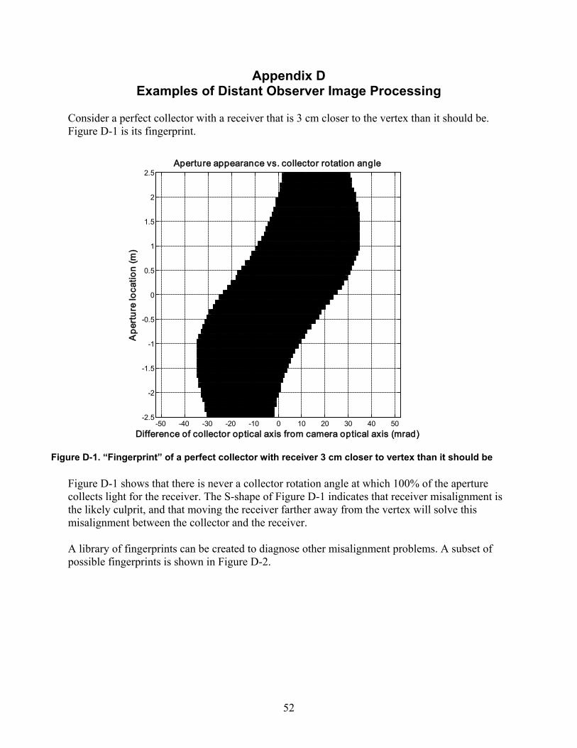
52

Appendix D Examples of Distant Observer Image Processing

Consider a perfect collector with a receiver that is 3 cm closer to the vertex than it should be. Figure D-1 is its fingerprint.

-50 -40 -30 -20 -10 0 10 20 30 40 50-2.5

-2

-1.5

-1

-0.5

0

0.5

1

1.5

2

2.5

Difference of collector optical axis from camera optical axis (mrad)

Ape

rtur

e lo

catio

n (m

)

Aperture appearance vs. collector rotation angle

Figure D-1 shows that there is never a collector rotation angle at which 100% of the aperture collects light for the receiver. The S-shape of Figure D-1 indicates that receiver misalignment is the likely culprit, and that moving the receiver farther away from the vertex will solve this misalignment between the collector and the receiver. A library of fingerprints can be created to diagnose other misalignment problems. A subset of possible fingerprints is shown in Figure D-2.

Figure D-1. “Fingerprint” of a perfect collector with receiver 3 cm closer to vertex than it should be

53

-50 0 50-2.5

-2

-1.5

-1

-0.5

0

0.5

1

1.5

2

2.5

Difference of collector optical axis from camera optical axis (mrad)

Ape

rtur

e lo

catio

n (m

)

Aperture appearance vs. collector rotation angle

-50 0 50-2.5

-2

-1.5

-1

-0.5

0

0.5

1

1.5

2

2.5

Difference of collector optical axis from camera optical axis (mrad)

Ape

rtur

e lo

catio

n (m

)

Aperture appearance vs. collector rotation angle

-50 0 50-2.5

-2

-1.5

-1

-0.5

0

0.5

1

1.5

2

2.5

Difference of collector optical axis from camera optical axis (mrad)

Ape

rtur

e lo

catio

n (m

)

Aperture appearance vs. collector rotation angle

-50 0 50-2.5

-2

-1.5

-1

-0.5

0

0.5

1

1.5

2

2.5

Difference of collector optical axis from camera optical axis (mrad)

Ape

rtur

e lo

catio

n (m

)

Aperture appearance vs. collector rotation angle

-50 0 50-2.5

-2

-1.5

-1

-0.5

0

0.5

1

1.5

2

2.5

Difference of collector optical axis from camera optical axis (mrad)

Ape

rtur

e lo

catio

n (m

)

Aperture appearance vs. collector rotation angle

-50 0 50-2.5

-2

-1.5

-1

-0.5

0

0.5

1

1.5

2

2.5

Difference of collector optical axis from camera optical axis (mrad)

Ape

rtur

e lo

catio

n (m

)

Aperture appearance vs. collector rotation angle

The discussion until this point has focused on a perfect collector, i.e., a collector with no slope error. Real collectors have a slope error transverse and longitudinal to the focal line. Figure D-3 shows slope errors reasonably expected for parabolic trough collectors in service, with a transverse RMS value of 4 mrad and longitudinal value of 2 mrad. For this example, the orthogonal slope errors have been arbitrarily placed in phase.

receiver 3 cm farther away

receiver 3 cm to the right

receiver 3 cm to the left

receiver 3 cm farther away and 3 cm to right

receiver 3 cm farther away and 3 cm to left

receiver 4 cm too close and 2 cm to left

Figure D-2. Subset of “fingerprint” library that can be used to diagnose receiver misalignment

54

-2.5 -2 -1.5 -1 -0.5 0 0.5 1 1.5 2 2.5-10

-8

-6

-4

-2

0

2

4

6

8

10

Aperture location (m)

Slo

pe e

rror

(mra

d)Collector slope error

TransverseLongitudinal

We repeat the analysis, substituting the slope errors in Figure D-3 for the perfect collector previously assumed. Figure D-4 shows the fingerprint of a real collector with the receiver in perfect position along the focal line.

Figure D-3. Typical collector slope error

55

-50 -40 -30 -20 -10 0 10 20 30 40 50-2.5

-2

-1.5

-1

-0.5

0

0.5

1

1.5

2

2.5

Difference of collector optical axis from camera optical axis (mrad)

Ape

rtur

e lo

catio

n (m

)

Aperture appearance vs. collector rotation angle

Comparing Figure D-4 with Figure 15, we see that the slope errors significantly change the shape of the fingerprint. Additionally, as seen in the above plot, they can prevent a 100% acceptance band. The mirror panels could be adjusted to better focus light on the receiver and create this 100% acceptance band. The presence of slope errors will complicate the receiver and collector misalignment diagnosis, but it will still be possible. Figure D-5 shows that same six misalignment cases presented in Figure D-2 with collector slope error. The general trends of each fingerprint can still be recognized.

Figure D-4. Collector with typical collector slope error and receiver in perfect alignment

56

-50 0 50-2.5

-2

-1.5

-1

-0.5

0

0.5

1

1.5

2

2.5

Difference of collector optical axis from camera optical axis (mrad)

Ape

rtur

e lo

catio

n (m

)

Aperture appearance vs. collector rotation angle

-50 0 50-2.5

-2

-1.5

-1

-0.5

0

0.5

1

1.5

2

2.5

Difference of collector optical axis from camera optical axis (mrad)

Ape

rtur

e lo

catio

n (m

)

Aperture appearance vs. collector rotation angle

-50 0 50-2.5

-2

-1.5

-1

-0.5

0

0.5

1

1.5

2

2.5

Difference of collector optical axis from camera optical axis (mrad)

Ape

rtur

e lo

catio

n (m

)

Aperture appearance vs. collector rotation angle

-50 0 50-2.5

-2

-1.5

-1

-0.5

0

0.5

1

1.5

2

2.5

Difference of collector optical axis from camera optical axis (mrad)

Ape

rtur

e lo

catio

n (m

)

Aperture appearance vs. collector rotation angle

-50 0 50-2.5

-2

-1.5

-1

-0.5

0

0.5

1

1.5

2

2.5

Difference of collector optical axis from camera optical axis (mrad)

Ape

rtur

e lo

catio

n (m

)

Aperture appearance vs. collector rotation angle

-50 0 50-2.5

-2

-1.5

-1

-0.5

0

0.5

1

1.5

2

2.5

Difference of collector optical axis from camera optical axis (mrad)A

pert

ure

loca

tion

(m)

Aperture appearance vs. collector rotation angle

One last caveat in this analysis is that it assumes that the receiver image as seen in the trough aperture is uniform and consistent along the length of the trough. In reality, the optical shape of trough apertures are not constant along the trough length. The receiver shape and position also are not constant along the module length due to sag, bending, bowing, etc. This all results in receiver image coverage changing along the length of the trough. Aerial imagery in theory can capture all of this information, but it is a significant task to process this amount of data to provide this level of quantitative analysis for an entire field.

receiver 3 cm farther away

receiver 3 cm to the right

receiver 3 cm to the left

receiver 3 cm farther away and 3 cm to right

receiver 3 cm farther away and 3 cm to left

receiver 4 cm too close and 2 cm to left

Figure D-5. Repeat of analysis in Figure D-2 but with typical collector slope error

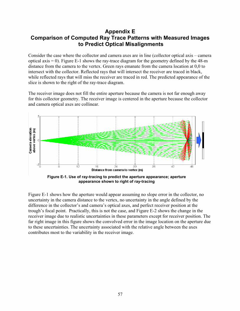
57

Appendix E Comparison of Computed Ray Trace Patterns with Measured Images

to Predict Optical Misalignments Consider the case where the collector and camera axes are in line (collector optical axis – camera optical axis = 0). Figure E-1 shows the ray-trace diagram for the geometry defined by the 48-m distance from the camera to the vertex. Green rays emanate from the camera location at 0,0 to intersect with the collector. Reflected rays that will intersect the receiver are traced in black, while reflected rays that will miss the receiver are traced in red. The predicted appearance of the slice is shown to the right of the ray-trace diagram. The receiver image does not fill the entire aperture because the camera is not far enough away for this collector geometry. The receiver image is centered in the aperture because the collector and camera optical axes are collinear.

Figure E-1 shows how the aperture would appear assuming no slope error in the collector, no uncertainty in the camera distance to the vertex, no uncertainty in the angle defined by the difference in the collector’s and camera’s optical axes, and perfect receiver position at the trough’s focal point. Practically, this is not the case, and Figure E-2 shows the change in the receiver image due to realistic uncertainties in these parameters except for receiver position. The far right image in this figure shows the convolved error in the image location on the aperture due to these uncertainties. The uncertainty associated with the relative angle between the axes contributes most to the variability in the receiver image.

Figure E-1. Use of ray-tracing to predict the aperture appearance; aperture appearance shown to right of ray-tracing

58

Now that the uncertainty between the photographs and ray-tracing has been quantified, ray-trace results can be compared with the receiver position slices of Figure 26 to see if the receiver is properly aligned to the collector. Figure E-3 compares ray-trace results with the receiver position results of the middle (M) slice for -1°, 0°, 1°, 2°, and 3° relative angles between the collector optical axis and the camera optical axis.

Figure E-2. Uncertainty in receiver image edge position due to uncertainties associated with slope error (3 mrad), distance from camera to vertex (± 1 m), and

the relative alignment between the axes (±0.5°)

59

The photograph receiver image results do not match the ray-trace results in Figure E-3, even accounting for the variability in the receiver image due to slope error, distance and angular uncertainty. The remaining parameter is the receiver position – perhaps the receiver is not placed exactly at the focal point. Figure E-4 repeats the ray-trace but for four different receiver positions, as shown in the diagram.

Figure E-3. Comparing ray-trace receiver image results for a collector with the receiver at the focal point to the receiver image

results obtained from the photographs for the middle slice

60

The fourth panel (bottom right) best agrees with the observed receiver images. In this panel, the receiver was located one receiver diameter (Dtube) below the optical axis. Figure E-5 compares this image directly with the observed middle slice pattern and includes the variability of the receiver image due to slope error and geometrical uncertainty.

Figure E-4. Receiver is moved away from the focal point by 7 cm (1 receiver diameter) in four different directions, and the resulting simulated receiver image from the ray-trace

61

The ray-trace results for a receiver 7 cm below the optical axis, as shown in panel 4 in Figure E-4, match the middle slice photograph results within uncertainty. This indicates that the real receiver is low by about 7 cm. Similar studies were performed on the left and right slices. Results indicate that the left slice is 5 cm below the optical axis and 2 cm too far away from the vertex, and the right slice is 3 cm below the optical axis and 1 cm too far away from the vertex.

Figure E-5. Comparison of ray-tracing receiver image results for a collector with the receiver 7 cm below the optical axis with the receiver images taken from the photographs. This good match between results

indicates that the real receiver is low by about 7 cm.

F1147-E(10/2008)

REPORT DOCUMENTATION PAGE Form Approved OMB No. 0704-0188

The public reporting burden for this collection of information is estimated to average 1 hour per response, including the time for reviewing instructions, searching existing data sources, gathering and maintaining the data needed, and completing and reviewing the collection of information. Send comments regarding this burden estimate or any other aspect of this collection of information, including suggestions for reducing the burden, to Department of Defense, Executive Services and Communications Directorate (0704-0188). Respondents should be aware that notwithstanding any other provision of law, no person shall be subject to any penalty for failing to comply with a collection of information if it does not display a currently valid OMB control number. PLEASE DO NOT RETURN YOUR FORM TO THE ABOVE ORGANIZATION. 1. REPORT DATE (DD-MM-YYYY)

February 2009 2. REPORT TYPE

Management Report 3. DATES COVERED (From - To)

4. TITLE AND SUBTITLE

Assess the Efficacy of an Aerial Distant Observer Tool Capable of Rapid Analysis of Large Sections of Collector Fields: FY 2008 CSP Milestone Report, September 2008

5a. CONTRACT NUMBER DE-AC36-08-GO28308

5b. GRANT NUMBER

5c. PROGRAM ELEMENT NUMBER

6. AUTHOR(S) G. Jorgensen, F. Burkholder, A. Gray, and T. Wendelin

5d. PROJECT NUMBER NREL/MP-550-44332

5e. TASK NUMBER CP07.1001

5f. WORK UNIT NUMBER

7. PERFORMING ORGANIZATION NAME(S) AND ADDRESS(ES) National Renewable Energy Laboratory 1617 Cole Blvd. Golden, CO 80401-3393

8. PERFORMING ORGANIZATION REPORT NUMBER NREL/MP-550-44332

9. SPONSORING/MONITORING AGENCY NAME(S) AND ADDRESS(ES)

10. SPONSOR/MONITOR'S ACRONYM(S) NREL

11. SPONSORING/MONITORING AGENCY REPORT NUMBER

12. DISTRIBUTION AVAILABILITY STATEMENT National Technical Information Service U.S. Department of Commerce 5285 Port Royal Road Springfield, VA 22161

13. SUPPLEMENTARY NOTES

14. ABSTRACT (Maximum 200 Words) We assessed the feasibility of developing an aerial Distant Observer optical characterization tool for collector fields in concentrating solar power plants.

15. SUBJECT TERMS Solar; CSP; collector field; optical characterization; Distant Observer; alignment

16. SECURITY CLASSIFICATION OF: 17. LIMITATION OF ABSTRACT

UL

18. NUMBER OF PAGES

19a. NAME OF RESPONSIBLE PERSON a. REPORT

Unclassified b. ABSTRACT Unclassified

c. THIS PAGE Unclassified 19b. TELEPHONE NUMBER (Include area code)

Standard Form 298 (Rev. 8/98) Prescribed by ANSI Std. Z39.18