Final Report:

Arizona Public Service Wind Integration Cost Impact Study

Prepared for Arizona Public Service Company Prepared by

Principal Investigator: Dr. Tom Acker, Department of Mechanical Engineering September 2007

i

PREFACE The purpose of this report is to describe the methods employed and results obtained in a wind integration cost impact analysis conducted for the Arizona Public Service Company (APS). This study was conducted under the direction of the Sustainable Energy Solutions Group at Northern Arizona University (NAU) under contract with APS. Important contributions to this work were provided by NAU, APS, EnerNex Corporation, and 3TIER. The contributing authors to this report were: Tom Acker, Ph.D., Associate Professor of Mechanical Engineering, Northern Arizona University Jason Buechler, Graduate Research Assistant, Northern Arizona University Scott Broome, Graduate Research Assistant, Northern Arizona University Cameron Potter, Ph.D., Power Prediction Engineer, 3TIER Hugo Gil, Ph.D., Research Scientist, 3TIER Bob Zavadil, Principal Consultant, EnerNex Corporation Jerry Melcher, Consultant, EnerNex Corporation Ron Flood, Technical Consultant, Arizona Public Service Company Marcus Schmidt, Marketing and Trading Ops Planning Section Leader, APS Richard La Peter, Senior Engineer with Resource Analysis, APS The authors would like to thank the following people and groups for their valuable contributions in providing information, reviewing methods, or providing feedback during the course of the project: Michael Milligan, Ph.D., Consultant to the National Renewable Energy Laboratory Debra Lew, Ph.D., National Renewable Energy Laboratory Brian Parsons, National Renewable Energy Laboratory J. Charles Smith, Utility Wind Integration Group Harvey Boyce, Arizona Power Authority Brad Albert, Arizona Public Service Company Guillermo Maese, Marketing and Trading Technical Services Manager, APS Pat Dinkel, Arizona Public Service Company Barbara Lockwood, Arizona Public Service Company Eran Mahrer, Arizona Public Service Company

ii

TABLE OF CONTENTS

Preface.................................................................................................................................. i Table of Contents................................................................................................................ ii List of Figures .................................................................................................................... iii List of Tables ..................................................................................................................... vi Executive Summary.......................................................................................................... vii I. Introduction ......................................................................................................................1

Background Information..........................................................................................1 Project Objectives and Overview.............................................................................5 Project Team ............................................................................................................7 Report Organization.................................................................................................8

II. APS System Characterization .........................................................................................9 APS System Generation Resources and Loads........................................................9 APS System in 2010 ..............................................................................................12 Market Setup and System Operation .....................................................................13 Role of Transmission in Study...............................................................................16

III. Arizona Wind Resource Modeling and Results...........................................................17 3TIER Meso-Scale Wind Modeling ......................................................................19 Results of Meso-Scale Wind Model ......................................................................22 Wind Power Plant Modeling..................................................................................24 Results of Wind Power Modeling..........................................................................28

IV. Wind Integration Impact Analysis and Results ...........................................................43 Wind Power Impacts on System Operation and Costs ..........................................43 Wind Integration Primer ........................................................................................43 Ancillary Services for Power System Reliability , Security, and Power Quality..44 Ancillary Service Requirements for Wind Generation..........................................45 Assessments of Ancillary Service Requirements and Impacts on Power System Operations ..............................................................................................................46 Where do Ancillary Services “Come From”?........................................................47 Modeling of Wind Integration Impacts on the APS System..................................48 Wind Generation Impacts Within the Hour and Day Ahead .................................54 Incremental Regulating Reserves ..........................................................................54 Hour Ahead “Firmness”.........................................................................................56 Day Ahead “Firmness” ..........................................................................................58 Results of Modeling...............................................................................................59 Base Case and Reference Case Parameters ...........................................................59 Integration Cost Results.........................................................................................60

V. Conclusions...................................................................................................................68 Glossary .............................................................................................................................70 Appendix A........................................................................................................................72

Advisory Group Members .....................................................................................72 Appendix B ........................................................................................................................74

Maps of Installed MW of Wind Power for Each Study Scenario..........................74 References..........................................................................................................................76

iii

L IST OF FIGURES

Figure ES 1 – Regions within which wind power plants were considered for the purpose of this study, shown on the 2003 Arizona high-resolution map of wind energy at 50-meters above the ground....................................................................................................................... x Figure ES 2 - Wind power density map of the West (APA) modeling zone at 80-meters above the ground. .............................................................................................................................. xii Figure ES 3 – Wind power density map of the East modeling zone at 80-meters above the ground. ................................................................................................................................... xiii Figure ES 4 – Sensitivity of integration cost to percent penetration of wind energy, under base case assumptions.......................................................................................................... xviii Figure ES 5 – Sensitivity of integration cost to geographic diversity of wind energy, under base case assumptions............................................................................................................ xix Figure 1 – Time scales of importance when considering power system impacts of integrating wind energy (source: National Renewable Energy Laboratory)............................................... 2 Figure 2 – Overall perspective of the value derived from integrating wind into a utility system. ...................................................................................................................................... 3 Figure 3 – Regions within which wind power plants were considered for the purpose of this study, shown on the 2003 Arizona high-resolution map of wind energy at 50-meters above the ground. ................................................................................................................................ 4 Figure 4 – Bar chart illustrating the monthly variation of APS 2004 vs. 2006 actual own-system load.............................................................................................................................. 10 Figure 5 – Anticipated 2007 APS system energy mix, as produced by its generation resources. ................................................................................................................................ 10 Figure 6 – Dispatch stack of APS system resources to meet load during a typical summer day (CC = Combined Cycle Natural Gas, CT = Combustion Turbine, PPA = Power Purchase Agreement). ............................................................................................................................ 11 Figure 7 – The hourly load pattern for APS in 2004, scaled to meet the expected 2010 energy requirement and peak load. ..................................................................................................... 12 Figure 8 – Illustration of the APS high-voltage transmission system. ................................... 14 Figure 9 – Specific modeling zones for the meso-scale wind energy simulation................... 18 Figure 10 – Map with the nested model domain used in the simulation of the East zone. The innermost black box denotes the requested study area (simulated at a 5 km horizontal resolution, as shown by the black dots). ................................................................................. 21 Figure 11 – Wind power density map of the West (APA) modeling zone. ............................ 22 Figure 12 – Wind power density map of the East (APSCo) modeling zone. ......................... 23 Figure 13 – Wind speed maps of the two high resolution modeling zones: Aubrey Cliff (left) and Gray Mountain (right). ..................................................................................................... 24 Figure 14 – Example power curve from a wind turbine operating in a wind power plant (source: 3TIER). ..................................................................................................................... 25 Figure 15 – Turbine layout at the hypothetical wind power plant located near Bullhead City.................................................................................................................................................. 27

iv

Figure 16 - Example of turbine layout from a wind power plant, showing the links to the nearest NWP points: turbines are red, NWP points are blue and links are green. In the turbine layout shown here (not from the current study), the turbine locations were not set along straight lines. ........................................................................................................................... 27 Figure 17 – Modeled data traces at Aubrey Cliffs from the high resolution (1-km) data, contrasting the output from one turbine grouping with the output from the entire power plant.................................................................................................................................................. 28 Figure 18 – Average capacity factor at each wind power plant, computed using all turbine groups at each site for simulated years of 2003, 2004, and 2005. .......................................... 30 Figure 19 – Shaded contour plot of the capacity factor for scenario 4%-Med (4% wind energy and medium geographic diversity), showing how the capacity factor varies with hour of day and month of year. ....................................................................................................... 31 Figure 20 – Diurnal and seasonal capacity factor variations for the low, medium, and high geographic diversity cases for 4% wind energy penetration. ................................................. 31 Figure 21 – Average capacity factor for wind scenario 4%-Med, during APS’s expected highest 10% of load hours during 2010, and for all hours of 2010. ....................................... 32 Figure 22 – Ten-minute ramp histogram for ramping events greater than 10% of rated capacity in the West/APA region............................................................................................ 35 Figure 23 – Ten-minute ramp histogram for ramping events greater than 10% of rated capacity in the East/APS region.............................................................................................. 36 Figure 24 – Ten-minute ramps from the 5-km and 1-km resolution data for Aubrey Cliffs. . 37 Figure 25 – Ten-minute ramps from the 5-km and 1-km resolution data for Gray Mountain 38 Figure 26 – Hourly ramp histogram for ramping events greater than 10% of rated capacity in the West/APA region. ............................................................................................................. 40 Figure 27– Hourly ramp histogram for ramping events greater than 10% of rated capacity in the East/APS region. ............................................................................................................... 41 Figure 28 – Relationship between effects of variability and uncertainty, APS planning functions, and the ancillary services of unit commitment (UC), load following (LF) and regulation (Reg). ..................................................................................................................... 53 Figure 29 – APS 1-minute load sample and 20-minute rolling average trend........................ 55 Figure 30 – Expanded view of Figure 29................................................................................ 55 Figure 31 – Regulation characteristic resulting from subtracting the load trend from the 1-minute load data...................................................................................................................... 55 Figure 32 – Sensitivity of integration cost to percent penetration of wind energy, under base case assumptions..................................................................................................................... 63 Figure 33 – Sensitivity of integration cost to geographic diversity of wind energy, under base case assumptions..................................................................................................................... 64 Figure 34 – Sensitivity of integration cost to hour-ahead firmness, for both 4% and 10% wind energy penetration.......................................................................................................... 65 Figure 35 – Cost associated with variation in the hour-ahead firmness plotted versus the percent of wind energy considered non-firm hour ahead, for both 4% and 10% wind energy penetration............................................................................................................................... 66 Figure 36 – Sensitivity of integration cost to day-ahead firmness, for 10% wind energy penetration............................................................................................................................... 66 Figure 37 – Sensitivity of integration cost to day-ahead firmness, for 10% wind energy penetration............................................................................................................................... 67

v

Figure 38 – Cost of day-ahead firmness plotted versus the percent of wind energy considered non-firm day ahead, for both 4% and 10% wind energy penetration. .................................... 67 Figure B- 1: Installed MW at each simulated wind power plant, medium geographic diversity, for 1%, 4%, 7%, and 10% penetration by energy. .................................................. 75 Figure B- 2: Installed MW at each simulated wind power plant, for 4% wind energy penetration, under assumptions of High (H), Medium (M), and low (L) geographic diversity.................................................................................................................................................. 75

vi

L IST OF TABLES Table ES 1 – Matrix of wind energy penetration and geographic diversity scenarios considered. ............................................................................................................................... ix Table ES 2 – Megawatts (MW) of installed capacity from each site employed in the various scenarios considered. ............................................................................................................. xiv Table ES 3 – Matrix of wind integration scenarios considered with the associated integration costs listed in $/MWh. ............................................................................................................ xx Table 1 – Matrix of wind energy penetration and geographic diversity scenarios considered. 5 Table 2 – APS 2007 portfolio of generation resources........................................................... 10 Table 3 – Listing of the total installed nameplate capacity of wind turbines at each wind power plant.............................................................................................................................. 26 Table 4 – Megawatts (MW) of installed capacity from each site employed in the various scenarios considered. .............................................................................................................. 29 Table 5 – Summary of some key wind power statistics for the wind penetration and geographic diversity cases considered. ................................................................................... 29 Table 6 – Distribution of ten-minute ramps, sorted by wind power plant and grouped in percentages of rated capacity. ................................................................................................. 33 Table 7 – Distribution of hourly ramps, sorted by wind power plant and grouped in percentages of rated capacity. ................................................................................................. 38 Table 8 – Summary of amount of additional spinning reserve required to handle the wind energy on the APS system. ..................................................................................................... 56 Table 9 – Incremental Impact of Next-Hour Wind Generation Uncertainty (HA = Hour Ahead, MAE = Mean Absolute Error, St.Dev. = Standard Deviation, Delta = St. Dev. with wind – St. Dev. load only). ..................................................................................................... 57 Table 10 – Hour-ahead “Firmness” factors for 1%, 4%, 7% and 10% wind energy penetration scenarios considering load forecast error, assuming medium geographic diversity of the wind power plants. ........................................................................................................................... 58 Table 11 – A summary of the day-ahead firmness, hour-ahead firmness, and added spinning reserve used in RTSim for each of the wind energy scenarios being considered................... 59 Table 12 – Summary of integration costs from other recent wind integration studies, with the two of the APS medium geographic diversity cases added (source: UWIG). ........................ 64 Table 13 – Matrix of wind integration scenarios considered with the associated integration costs listed in $/MWh. ............................................................................................................ 65

vii

ARIZONA PUBLIC SERVICE WIND INTEGRATION COST IMPACT STUDY

EXECUTIVE SUMMARY

This report was produced by Northern Arizona University (NAU), with contributions

from EnerNex Corporation, 3TIER, and Arizona Public Service Company (APS). The report is a result of an eight month study to characterize the impacts and costs due to the variability and uncertainty of wind energy associated with integrating wind energy into APS’ utility resources and practices. Introduction Wind energy brings many positive benefits to the utility system, such as cost effective energy, long-term price stability, and some system capacity, but it also has different generation characteristics than conventional utility resources. In particular, since the wind is driven by meteorological processes it is inherently variable. This variability occurs on all time frames of utility operation from real-time minute-to-minute fluctuations through yearly variation affecting long-term planning. Recent wind integration studies have demonstrated that the variations of most importance and cost are those in the hourly and daily timeframe, related to the ancillary services of load following and unit commitment. Regulation costs, incurred by fast responding units that respond to the random minute-to-minute fluctuations on the system, are also incurred but are smaller in magnitude. In addition to being variable, wind power production is also a challenge to accurately predict on the time scales of interest to utility planners and operators: day ahead and for long-term planning of system adequacy (i.e., meeting the system peak load during the year). Wind energy is more predictable in the hour-ahead time frame, but even then the uncertainty in wind forecasts must be accounted for in utility operation and dispatching. In order to minimize impacts and maximize benefits, each utility that incorporates wind energy must learn how to accommodate the uncertainty and variability of wind energy in their operational and planning practices, and do so while maintaining system reliability. The objectives of this study were to analyze operating impacts and costs of integrating various levels of wind energy in the APS balancing area (i.e., control area), due to the variability and uncertainty of wind energy. Specifically, attention was focused on the amount of wind energy the APS system may see in the relatively near term, and therefore would provide a fair integration cost to utilize in evaluating wind energy proposals in APS’s current and future RFP’s. The results obtained in any integration study are highly dependent on the input assumptions and analysis methods. The philosophy adopted by APS in this study was to determine a realistic, yet conservative, value for the integration cost (i.e., within the limitations of the modeling, come as close as possible to the actual integration cost without underestimating). Furthermore, the study process was devised to produce meaningful, broadly supported results through a technically rigorous, inclusive study process. Northern Arizona University was the

viii

lead organization in the study effort, working in collaboration with APS, EnerNex Corporation, and 3TIER. NAU was responsible for managing the project and for overall technical direction. EnerNex was the primary technical consultant on the integration analysis, 3TIER was responsible for the wind speed and power modeling, and APS was responsible for system characterization and modeling. There were two important advantages in APS performing the modeling: 1) they are experts in modeling and running their system, and best suited to model system operation; and 2) they gained an increased understanding of wind energy and its generation characteristics, and developed in-house expertise to conduct future integration cost impact studies. A Technical Advisory Group (TAG) was formed to provide external review and guidance to the study), and in particular were counted upon to assist in selecting key model assumptions and parameters used in the study. The project team and TAG were assembled so as to build upon prior wind integration studies and related technical work, to coordinate with recent and current regional power system study work, and to ensure that the assumptions and methods employed were appropriate. The public was informed of the study through stakeholder meetings conducted jointly by APS and NAU, and supported by the project team. Through the stakeholder meetings, the project team sought interaction and input regarding all aspects of the project, including wind resources, technical details, and policy ramifications. The organizations invited to the stakeholder meetings were also expected to serve as conduits of information to the people and organizations they represented. Study Set-up A critical aspect of any wind integration study is correctly accounting for the relationship between wind and load. System load is partly dictated by the weather, such as when hot weather causes high air conditioning loads. Wind power generation is obviously related to the weather, and so there will be some correlation between the weather, the load, and the wind power. In order to correctly capture this relationship in an integration study, a time-series of historical load data is matched with either the historical wind power data or a simulation of the wind power data. For the purpose of this study, APS 2004 hourly load data was employed in conjunction with simulated wind power production data over the same period. The study year was selected as 2010 so that the integration analysis could be conducted while knowing with some certainty the characteristics of the APS loads and generation resources. Thus, the 2004 loads were scaled-up to the level expected in 2010. A wind power simulation was conducted by 3TIER, using a meso-scale weather model employing 2004 historical weather data as an input. The idea here was that the meso-scale model does a good job predicting and downscaling the wind speed, air density, etc., when using the historical coarse resolution weather data to maintain a high correlation between the simulations and the actual weather. This type of predictive model using historical weather data is called a “backcast.” The wind speed data was then turned into wind power production through an algorithm that assumes a turbine type, makes reasonable assumptions about the wind power plant layout, and produces a simulated power output for several distinct wind power plants. For this study, a GE 1.5sl turbine (1.5 MW rated output) with a 77-meter rotor diameter and 80-meter hub height was the turbine model employed at all locations. Wind power output from the turbines was adjusted to account for the local air density, which is lower at higher elevations. Key elements of this simulation were that the wind power

ix

prediction is correlated to the weather and any correlation with the load is implicitly captured, and that the variability of the wind power output is typical of what is actually realized at functioning wind power plants. A range of wind energy penetration levels and geographic diversity in wind power production were considered, as shown in Table ES 1. All wind energy penetration levels listed refer to the expected APS energy production and peak load in 2010. In this table, “energy penetration” implies a percentage of the APS system energy consumption (estimated at approximately 34,600,000 MWh in 2010) provided by wind energy, and “penetration by capacity” is determine by dividing the MW capacity of wind power by the APS peak system load in 2010 (estimated at 7,905 MW). The “X” in the center of this table indicates that the 4% wind energy penetration, medium diversity case was considered the “base case” in this study. This was selected as the base case because it is a reasonable approximation of what may be achieved over the relatively near term in Arizona. The locations and sizes of the wind power plants simulated were determined as part of the project. Wind power plants were located in such a way that the prescribed level of energy and geographic diversity could be achieved (e.g., high, medium, or low), and so that the wind power plants would be located at sites within the zones where an adequate wind power potential existed as predicted by the simulation (minimum of a class 3 wind resource).

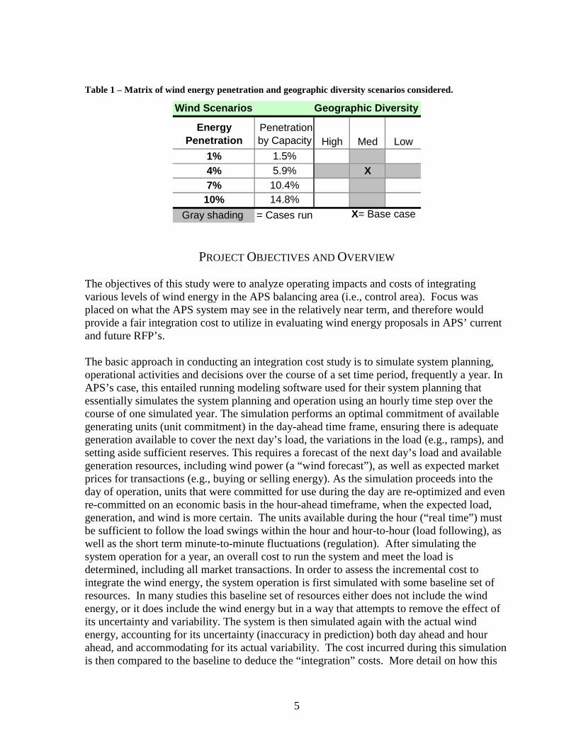
Table ES 1 – Matrix of wind energy penetration and geographic diversity scenarios considered.

Wind Scenarios Geographic Diversity

Energy Penetration

Penetration by Capacity High Med Low

1% 1.5%4% 5.9% X7% 10.4%

10% 14.8%

Gray shading = Cases run X= Base case For the purpose of this study, wind power plants were considered in Arizona within the two zones shown on the 2003 high resolution Arizona wind energy map displayed in Figure ES 1 (for more information about the wind map, visit the Northern Arizona University Sustainable Energy Solutions website: http://wind.nau.edu/maps/). The more colorful areas shown on the map correspond to better wind resource areas, most of which are contained within the two zones. Furthermore, locating wind power plants in both of these zones allows geographic diversity in siting the plants, similar to what could be achieved in the state. To summarize, the overall objective of this study is to compute the incremental integration costs incurred by the APS system in accommodating the variability and uncertainty of wind energy. This was accomplished as follows:

x

Figure ES 1 – Regions within which wind power plants were considered for the purpose of this study, shown on the 2003 Arizona high-resolution map of wind energy at 50-meters above the ground.

West Zone

East Zone

Dr. Tom Acker Tom.Acker@nau.edu

xi

• Simulate APS system operation and planning for one typical year: o Determine the operating costs for the system excluding the effects of wind

variability and uncertainty. o Determine the operating costs for the system with the actual wind, including

the effects of its variability and uncertainty. o Deduce the integration costs as the difference between the costs computed in

these two simulations. • The study year was selected as 2010. • Historical load data for APS in 2004 was scaled to match the expected load and

energy required in 2010, maintaining the hour-to-hour shape of the load and its correlation to the weather.

• A reasonable set of wind power plants in Arizona were simulated, using a meso-scale weather model, 2004 historical weather data, and a wind power prediction model. This provided wind power data that is time-synchronized with the load data, maintaining any correlation inherent between the two.

• GE 1.5 MW wind turbines with a 77-m rotor diameter and an 80-m hub height were assumed in the wind power plant modeling.

• The sensitivity of wind integration costs to wind energy penetration and geographic diversity was investigated as indicated in Table ES 1.

Wind Modeling Analysis and Results There were two basic requirements for the wind energy modeling as used in this wind integration study: 1) it be physics-based and of sufficient resolution in both time and space to accomplish the goals of the integration study; and 2) it accurately convert wind speed information to wind power production data, including the correct characterization of the variability exhibited in the output of the wind power plants. As to this later point, because the wind speed and direction varies even over small areas, no two wind turbines see the same input wind speed nor have identical power output. Further, each wind turbine possesses a significant amount of inertia, hence its output cannot respond to the faster fluctuations of the wind speed. For these reasons, one cannot simply take the output of a meso-scale wind model (or wind anemometer data) and run it directly through a manufacturer’s turbine power curve to accurately estimate the power output for an entire wind power plant. There must be some method to ensure that the variability of modeled wind plant output emulates the output that is actually realized in operational wind power plants. Given these considerations, the following parameters were defined for the wind modeling in consultation with the project technical advisory group:

• Wind speeds were simulated with 3TIER’s meso-scale model throughout the zones shown in Figure ES 1, for the historical years of 1996 to 2006, with particular focus on 2003, 2004, and 2005.

• The East and West zones demarked by the blue and red boxes in this figure were both modeled using a grid spacing of 5-km (the meso-scale model predicts wind speed, direction, air density, etc., at pre-defined grid points), for the historical period 1996 to 2006.

• Two smaller zones, approximated by the small black rectangles in Figure ES 1, were selected for additional higher-resolution modeling with 1-km grid spacing. These

xii

zones are the Aubrey Cliffs, north of Seligman, and Gray Mountain, west of Cameron, and are known to have good potential for wind resource development, but also have highly variable topography. Because a 5-km resolution simulation may not adequately capture the effects of the topographical features present in these areas, more refined 1-km resolution simulations were conducted. The higher resolution zones were modeled only for historical years 2003, 2004, and 2005.

• The time-step of the meso-scale simulation was 10-minutes (for all zones). This resolution in time allows study of the intra-hour wind variations, and can easily be modified for an hourly power system simulation.

• Wind speed and related meteorological parameters were predicted at 50-m, 80-m, and 100-m above the ground at each model grid point.

Maps displaying the results of the meso-scale wind simulation for the West and East modeling zones are displayed in Figure ES 2 and Figure ES 3. Each map displays the wind power density (W/m2) at 80-meters above the ground since it is more directly indicative of the wind energy potential at a given site than the wind speed, and thus better suited to guide the selection of wind power plant locations. The wind class designations shown on the scale correspond to the mid-point of the wind class. Since class 3 is considered the minimum wind class that currently can support an economically feasible wind power plant, the areas where potential wind power plants could be located are colored light orange to dark red. It is worth recognizing that the base data used for creating these maps is the 5-km resolution data, and the smooth variation of the colors shown on this map resulted from applying an interpolating

Figure ES 2 - Wind power density map of the West (APA) modeling zone at 80-meters above the ground.

xiii

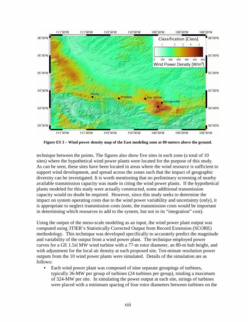
Figure ES 3 – Wind power density map of the East modeling zone at 80-meters above the ground.

technique between the points. The figures also show five sites in each zone (a total of 10 sites) where the hypothetical wind power plants were located for the purpose of this study. As can be seen, these sites have been located in areas where the wind resource is sufficient to support wind development, and spread across the zones such that the impact of geographic diversity can be investigated. It is worth mentioning that no preliminary screening of nearby available transmission capacity was made in citing the wind power plants. If the hypothetical plants modeled for this study were actually constructed, some additional transmission capacity would no doubt be required. However, since this study seeks to determine the impact on system operating costs due to the wind power variability and uncertainty (only), it is appropriate to neglect transmission costs (note, the transmission costs would be important in determining which resources to add to the system, but not in its “integration” cost). Using the output of the meso-scale modeling as an input, the wind power plant output was computed using 3TIER’s Statistically Corrected Output from Record Extension (SCORE) methodology. This technique was developed specifically to accurately predict the magnitude and variability of the output from a wind power plant. The technique employed power curves for a GE 1.5sl MW wind turbine with a 77-m rotor diameter, an 80-m hub height, and with adjustment for the local air density at each proposed site. Ten-minute resolution power outputs from the 10 wind power plants were simulated. Details of the simulation are as follows:

• Each wind power plant was composed of nine separate groupings of turbines, typically 36-MW per group of turbines (24 turbines per group), totaling a maximum of 324-MW per site. In simulating the power output at each site, strings of turbines were placed with a minimum spacing of four rotor diameters between turbines on the

xiv

same string and a minimum spacing of 10 rotor diameters between the rows of turbines.

• The 10-minute wind power output from the SCORE methodology was aggregated into hourly power sequences for each scenario for input into the APS power system model.

• Wind power output from all 10 sites shown in Figure ES 2 and Figure ES 3 were employed for the high geographic diversity case. For the medium diversity cases, output from wind power plants from three sites centrally located in the state was used (those with blue circles in Figure ES 2). For the low diversity case, output from only two wind power plants were employed (those with yellow circles in Figure ES 2).

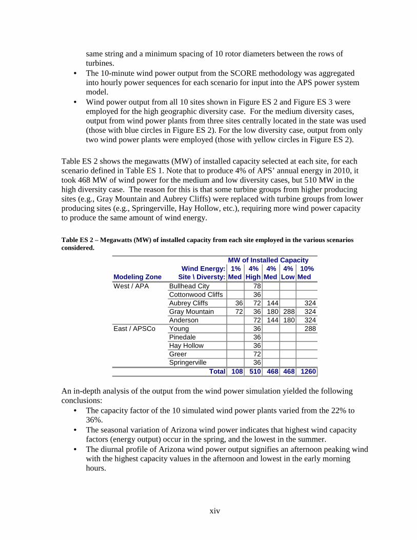
Table ES 2 shows the megawatts (MW) of installed capacity selected at each site, for each scenario defined in Table ES 1. Note that to produce 4% of APS’ annual energy in 2010, it took 468 MW of wind power for the medium and low diversity cases, but 510 MW in the high diversity case. The reason for this is that some turbine groups from higher producing sites (e.g., Gray Mountain and Aubrey Cliffs) were replaced with turbine groups from lower producing sites (e.g., Springerville, Hay Hollow, etc.), requiring more wind power capacity to produce the same amount of wind energy.

Table ES 2 – Megawatts (MW) of installed capacity from each site employed in the various scenarios considered.

MW of Installed CapacityWind Energy: 1% 4% 4% 4% 10%

Modeling Zone Site \ Diversty: Med High Med Low MedWest / APA Bullhead City 78

Cottonwood Cliffs 36Aubrey Cliffs 36 72 144 324Gray Mountain 72 36 180 288 324Anderson 72 144 180 324

East / APSCo Young 36 288Pinedale 36Hay Hollow 36Greer 72Springerville 36

Total 108 510 468 468 1260 An in-depth analysis of the output from the wind power simulation yielded the following conclusions:

• The capacity factor of the 10 simulated wind power plants varied from the 22% to 36%.

• The seasonal variation of Arizona wind power indicates that highest wind capacity factors (energy output) occur in the spring, and the lowest in the summer.

• The diurnal profile of Arizona wind power output signifies an afternoon peaking wind with the highest capacity values in the afternoon and lowest in the early morning hours.

xv

• The capacity value of an Arizona wind resource located in the regions modeled in this study will likely be a significant fraction of, but less than, its annual capacity factor.

• The vast majority of 10-minute ramping events are less than 10% of the wind power plant capacity. The combined output from all wind power plants is considerably smoother than any of the individual power plants.

• Large ramp events (larger than 10% of nameplate) at the hourly timescale take place about 15% of the time for individual wind power plants, and about 5% of the time for geographically diverse wind power production. Geographical diversity results in some smoothing of large ramps.

Wind Integration Analysis Technique The basic approach in conducting this integration cost study was to simulate system planning, operational activities and decisions over the course of a set time period. In APS’s case, this entailed running the modeling software RTSimi over the course of one simulated year. RTSim is the tool used by APS on a daily basis to model their system planning and operation, and uses an hourly time step. The simulation performs an optimal commitment of available generating units (unit commitment) in the day-ahead time frame, ensuring there is adequate generation available to cover the next day’s load, the variations in the load (e.g., ramps), and setting aside sufficient reserves. As the simulation proceeds into the day of operation, units that were committed for use during the day are re-optimized and even re-committed on an economic basis in the hour-ahead timeframe, when the expected load, generation, and wind is more certain. The units available during the hour (“real time”) must be sufficient to follow the load swings within the hour and hour-to-hour (load following), as well as the short term minute-to-minute fluctuations (regulation). After simulating the system operation for a year, an overall cost to run the system and meet the load is determined, including all market transactions. In order to assess the incremental cost to integrate the wind energy, the system operation is first simulated with some baseline set of resources that does include the wind energy but in a way that attempts to remove the effect of its uncertainty and variability. The system is then simulated again with the actual wind energy, accounting for its uncertainty (inaccuracy in prediction) both day ahead and hour ahead, and accommodating for its actual variability. The cost incurred during this simulation is then subtracted from the cost incurred with the baseline resources to deduce the “integration” costs. The integration cost depends upon the variability and output of the wind power, the variability and magnitude of the load, and the characteristics of the generation. APS is a summer-peaking utility with its peak driven primarily by residential customer growth and the associated cooling loads. As the customer base grows, the summer period load grows at a faster rate than the winter and shoulder months. In meeting its load obligation, APS employs a mix of generation resources. The base load resources are coal and nuclear and contribute about 2/3 of the energy requirement, while only accounting for about 1/3 of the capacity. The remaining 1/3 of the energy is supplied by gas-fired intermediate and peaking resources.

i RTSim is a production cost simulation model developed by Simtec in Madison, Wisconsin (see rtsim.com). It is an hourly simulation tool that can perform comprehensive simulation and optimization.

xvi

When APS employs its generation resources, it does so in the most economical way, typically utilizing the least expensive of its resources possible. Integration cost in this study was defined as the difference between the actual production cost incurred to serve the net of actual load and actual wind generation and the production cost from the reference case, where wind is perfectly known and adds no variability to the control area, and where next-day load is the only uncertainty. The basic method for determining the costs at the hourly level developed in previous studies proceeds as follows:

1) Run the unit commitment program in “optimization” mode to develop a plan for serving the forecasted load. Wind generation for the day is known perfectly, and is delivered in some predescribed pattern (either a flat block with equal amounts each hour throughout the day, or some diurnal distribution). Save the unit commitment as the starting point for the next case.

2) Using the unit commitment from 1), re-run the day with forecast load replaced by actual load. Do not allow the program to re-optimize, but allow it to re-dispatch available units to meet the actual load. Manually commit generation to meet load that cannot be served from the previous day commitment. Save the total production cost for the period and define it as the “reference production cost”

3) Repeat Step 1) with a next-day hour-by-hour wind generation forecast. Save the unit commitment as the starting point for the next case.

4) Using the unit commitment from 3), re-run the day with forecast load and forecast wind generation replaced by actual load and actual wind generation. Do not allow the program to re-optimize. Ensure the operating reserves have been appropriately incremented to account for the additional variability of wind generation. Re-dispatch available units and manually commit off-line units to meet the control area demand. Save the total production cost for the period and define it as the “actual production cost.”

5) Compute the integration cost as the difference between the “actual production cost” and the “reference production cost.”

Some modifications to the basic methodology outlined above were necessary to accommodate using RTSim. These included:

• Day-ahead load forecasts were automatically generated by the program, and therefore were not “historical” forecasts for the load pattern years from APS. RTSim generates a day-ahead forecast by averaging n days of (actual) hourly loads from its database, where n is a number of days defined by APS, typically less than 10. APS used n=1 for this modeling effort.

• Concerning wind energy forecasts, the version of RTSim utilized by APS at the time of the study would not allow any change in the actual wind that showed up during the day of operation from that which was forecast day ahead. The practical implication here was that the actual wind power time-series (from the simulation) had to be used for the forecasted wind, and that the impact of different wind forecasts could not be directly investigated (e.g., a professional forecast vs. a persistence forecast vs. a perfect forecast, etc.). In order to account for uncertainty in the day-ahead wind

xvii

forecast in the day-ahead optimization, RTSim allows a “firmness” factor to be applied to the wind energy. The firmness factor allows a fixed percentage between 0% and 100% of the forecasted wind generation for the day to be considered “firm” in the day-ahead optimization. The day-ahead firmness factor for all scenarios considered was selected as 60%. Therefore, RTSim would consider 60% of the wind forecasted for each hour to be firm and could be scheduled while the remaining 40% would not be counted on to serve load. RTSim’s optimization routine, therefore, always knows about the “shape” of the wind energy delivery for the next day, and the amount of wind energy delivered was always greater than what was forecast (unless a 100% firmness factor was used). The approach results in an over-commitment of conventional generating units on all days where wind energy delivery is not zero.

• Similar to the day-ahead forecast, RTSim requires the hour-ahead forecast of wind energy to be the same as the actual wind that shows up; however, an hour-ahead firmness factor can be set. By varying the hour-ahead firmness factor between 0% and 100%, the effect of uncertainty in the hour-ahead forecast can be deduced. The hour-ahead firmness factor varied for each scenario, depending on the specific wind power time-series at each site. Overall, the hour-ahead firmness factors varied from 85% (low geographic diversity) to 99% (low wind energy penetration), with a value of 87.5% for the base case of 4% wind energy and medium geographic diversity.

• Because RTSim is an hourly simulation model, it cannot by itself determine the amount of additional spinning reserve needed to accommodate the increased regulation due to the minute-to-minute fluctuations of the wind power. Using samples of 1-minute wind power data from an existing wind power plant and 1-minute APS load data, a calculation was performed to define the additional regulation burden due to wind energy. The range of additional spinning reserve required varied from 0.5 MW to 6.2 MW for 1% and 10% wind energy penetration, respectively (2.4 MW for the base case of 4% wind energy).

Certain aspects of the methodology listed above merit additional emphasis: • Load energy (MWh) and wind energy (MWh) delivered in “reference” and “actual”

cases are identical. If wind generation is assumed to be a “must take” resource, the payment from APS to the wind generators is identical in both the “reference” and “actual” cases. Therefore, the cost per MWh of wind energy is not relevant to the analysis (i.e., it “subtracts out”).

• Optimization cases are run with next-day forecast data. All binding decisions (unit commitment or de-commitment, day-ahead purchases, etc.) must be carried forward to the simulation of the actual day.

• Simulation cases are run with actual hourly load and wind data, and start from the optimized day-ahead plan. However, RTSim does allow a re-optimization of its available resources in the hour-ahead timeframe, based upon the generation resources set forth in the day-ahead commitment and those available within an hour of use (including resources on the market).

Finally, there is the issue of the wind generation attributes defined for the “reference” case. In this method, wind energy delivery is allowed to vary day-by-day and hour-by-hour. In the reference case, the wind energy is assumed to be 100% firm both day-ahead and hour-ahead

xviii

and therefore have no uncertainty. As will be discussed later, there is also no additional spinning reserve added to that required within each hour due to the wind in the reference case (thus no impact of the wind upon the within-hour regulation required in the reference case). The reference resource for wind assumed here is equivalent to an “as-available” energy contract with a third-party, where the terms of the contract allow the delivery to be scheduled a day in advance. Wind Integration Cost Impact Results Figure ES 4 shows the integration cost results for the medium geographic diversity case with 1%, 4%, 7% and 10% wind energy penetration. The overall height of each vertical bar on the chart signifies the full integration cost, with the colored sections of each bar indicating the proportion of the cost contributed by the regulation (added spinning reserve; green section), the hour-ahead uncertainty (hour-ahead firmness being less than 100%; red section), and the day-ahead uncertainty (day-ahead firmness being less than 100%; blue section). For the base case of 4% wind energy, the total integration cost is $3.25/MWh, varying from $0.91/MWh (1% wind energy) to $4.08/MWh (10% wind energy). Figure ES 5 displays the sensitivity of integration cost to geographic diversity, for the 4% wind penetration case. The center column on this chart corresponds to the base case and is identical to that shown in Figure ES 4. The main result demonstrated in this figure is the effect of geographic diversity on reducing the integration cost. As turbines are spread over a

1% 4% 7% 10%

Within-hour Regulating $0.40 $0.41 $0.31 $0.37

Hour-ahead Uncertainty $0.11 $1.88 $2.32 $2.65

Day-ahead Uncertainty $0.39 $0.95 $0.93 $1.06

$-

$0.50

$1.00

$1.50

$2.00

$2.50

$3.00

$3.50

$4.00

$4.50

Inte

gra

tio

n C

ost

$0.91

$3.25

$3.57

$4.08

Wind Energy Penetration

Base Case Assumptions:

DA firmness (60%)

HA firmness (87%)

Added spin (2.4 MW)

Figure ES 4 – Sensitivity of integration cost to percent penetration of wind energy, under base case assumptions.

xix

Case VI - Low

(Hrly Firm 84.5%)

Case III - Med

(Hrly Firm 87%)

Case I - High (Hrly

Firm 91.6%)

Within-hour Regulating $0.44 $0.41 $0.42

Hour-ahead Uncertainty $2.21 $1.88 $1.14

Day-ahead Uncertainty $0.66 $0.95 $1.04

$-

$0.50

$1.00

$1.50

$2.00

$2.50

$3.00

$3.50

Inte

gra

tio

n C

ost

$3.30 $3.25

$2.60

Diversity Case

Wind Penetration 4%

Base Case DA firmness (60%)

& added spin (2.4 MW)

Figure ES 5 – Sensitivity of integration cost to geographic diversity of wind energy, under base case assumptions.

broader geographic area, the variability in the output is reduced, both hour-to-hour and day-to-day. This effect is characterized in the hour-ahead firmness factor, which is highest for the high diversity case and lowest for the low diversity case. A summary of the integration costs for the full set of cases run is shown in Table ES 3. The primary conclusions from the integration cost study are as follows:

• Wind integration costs in the APS system, defined as the increase in operating costs due to the variability and uncertainty associated with wind generation divided by the total wind energy delivered, are consistent with results from other studies around the country. For APS, the costs range from just under $1.00/MWh of wind energy delivered at 1% penetration to just over $4.00/MWh at 10%.

• The integration costs of 4% wind energy (468 MW) in APS’ system (2010 peak load estimated at 7,905 MW) was estimate to be $3.25/MWh, with medium geographic diversity in locating wind turbine power plants in northern Arizona.

• Hour-ahead uncertainty, as employed by APS’ modeling tool RTSim for in-the-day commitment of generating units, is the largest component of integration cost. This quantity is effectively a type of operating reserve, and can be significant in magnitude relative to the other reserve amounts attributable to wind generation.

xx

• The beneficial effect of geographic diversity on reducing variations in aggregate wind energy production reduces integration costs.

• In RTSim, day-ahead forecasts of wind generation for unit commitment and scheduling are modeled as a firmness factor. The result of the sensitivity cases for firmness factors ranging from 0 to 100% show that a better, i.e., less costly, day-ahead plan is possible as more of the wind energy that is to be delivered can be accounted for in the unit commitment optimization. Conversely, if wind energy is ignored, more APS units are committed to operation than are actually needed, increasing operating costs.

• Because Arizona wind generation is high during the spring when the system load is only moderate and only a modest amount of flexible generation resources are required, this is the season during which the highest integration costs are incurred. Integration costs are lowest during the summer, when wind output is relatively light and virtually all of the flexible gas generation resources are on-line.

• Costs associated with gas supply imbalance were considered and found to be a small contributor to the total integration costs, in all cases less than $0.10 to $0.15/MWh. The cost is significant if there is either no day ahead forecast of the wind energy, or a very poor day ahead forecast. For any reasonable wind power forecast, the gas supply imbalance costs are quite small.

Table ES 3 – Matrix of wind integration scenarios considered with the associated integration costs listed in $/MWh.

Wind Scenarios Geographic Diversity

Energy Penetration

Penetration by Capacity High Med Low

1% 1.5% 0.914% 5.9% 2.60 3.25 3.307% 10.4% 3.5710% 14.8% 4.08

Gray Shading = Cases run Bold = Base Case

Integration Cost Summary ($/MWh)

1

I. INTRODUCTION

BACKGROUND INFORMATION Over the past decade, electrical energy derived from utility-scale wind turbines (>1 megawatt (MW) per turbine) has become more cost competitive relative to conventional electrical energy resources, especially natural-gas based generation. Furthermore, as the wind turbine technology has developed, the reliability of the turbines has become very high (>98% availability) and there is now significant experience in designing, financing, building and operating large wind power plants. As a result, the installed capacity of wind power has increased dramatically in the US over the past several years, from 2,500 MW in 2000 to over 11,500 MW in 2006.1 Worldwide there was over 74,000 MW installed at the end of 2006, and this significant growth is expected to continue over the next several years. In addition to its cost competitiveness, wind energy may bring other positive benefits such as long-term price stability, no emission of climate change gases, it requires no water, it is an indigenous resource, and it can foster rural economic development. Concurrent with the decreased cost and increased usage of wind energy, many states in the US have adopted policies to promote renewable-energy based electricity generation. One such example is the recently adopted Renewable Energy Standard and Tariff (REST) Rules passed by the Arizona Corporation Commission in November of 2006.2 One requirement of this rule is that an affected utility, such as Arizona Public Service Company (APS), should annually derive 5% of its energy from renewable energy resources by 2015, and 15% by 2025. Wind power is an eligible renewable energy generator under this rule, and because of its cost competitiveness, may be employed to provide a significant fraction of the renewable energy production required. While wind energy has many positive aspects, it also has different generation characteristics than conventional utility resources. In particular, since the wind is driven by meteorological processes it is inherently variable. This variability occurs on all time frames of utility operation from real-time minute-to-minute fluctuations through yearly variation affecting long-term planning. A conceptual view of these time frames is depicted in Figure 1. Recent wind integration studies have demonstrated that the variations of most importance and cost are those in the hourly and daily timeframe, related to the ancillary services of load following and unit commitment.3 In addition to being variable, it is also a challenge to accurately predict wind energy production on the time scales of interest to utility planners and operators: day ahead and for long-term planning of system adequacy (i.e., meeting the system peak load during the year). Wind energy is more predictable in the hour-ahead time frame, but even then the uncertainty in wind forecasts must be accounted for in utility operation and dispatching. In order to minimize impacts and maximize benefits, each utility that incorporates wind energy must learn how to accommodate the uncertainty and variability of wind energy in their operational and planning practices, and do so while maintaining system reliability.

2

Time (hour of day)0 4 8 12 16 20 24

Sys

tem

Loa

d (M

W)

seconds to minutes

Regulation

tens of minutes to hours

LoadFollowing

day

Scheduling

Figure 1 – Time scales of importance when considering power system impacts of integrating wind energy (source: National Renewable Energy Laboratory).

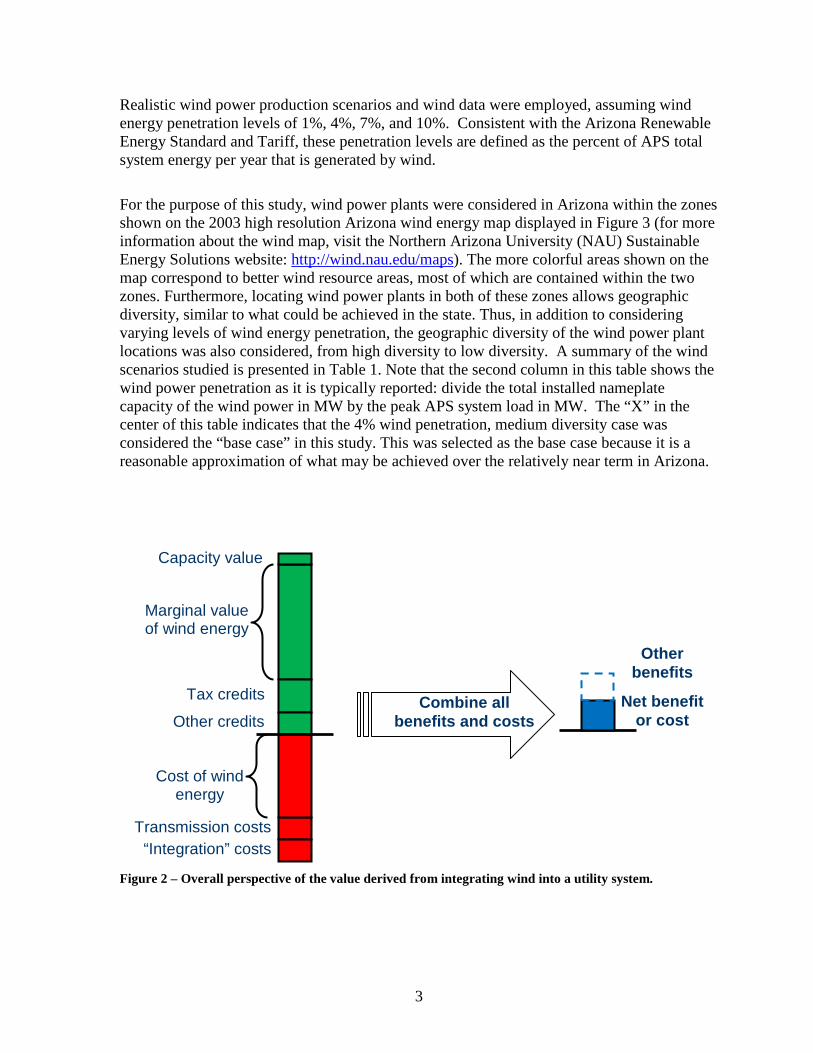
An overall perspective on the value of incorporating wind energy into a utility system is shown in Figure 2. The green bar shown represents the cumulative positive financial benefits of wind energy accrued over the course of a year, typically normalized per megawatt-hour (MWh) of wind energy production, the largest component of which is the marginal value of the wind energy. This marginal value is dependent upon when the wind blows and is higher during peak load hours and lower off-peak. The red bar shows the cumulative costs of incorporating wind energy. The dominant cost is the actual cost of the wind energy, which is typically purchased via a fixed-price, long-term contract. The “integration costs” shown on the bottom of the red bar is the additional cost incurred in planning and operation due to the uncertainty and variability of the wind energy. These additional costs are typically incurred as additional regulation and load following ancillary services, and in additional contingency reserves. Overall, there is generally a net benefit due to wind energy, represented by the blue bar in Figure 2, the magnitude of which varies from utility to utility based upon each system’s generation resources, load, wind resources, operational rules and constraints, and the market within which it operates. The “other benefits” shown correspond to non-monetized benefits, such as avoided carbon emissions, etc. An example wind integration study that considers the overall benefit of wind in a utility system is the recent study conducted by General Electric for the New York State Energy Research and Development Authority.4 When a utility considers purchasing renewable energy resources to meet a portfolio standard, it typically issues a “Request for Proposals” (RFP) and receives price proposals that specify a cost of energy, often inclusive of tax or other credits. In order to fairly compare these price proposals, it is necessary to understand and account for the “integration” costs associated with each resource. It was the goal of this study to determine a value for the integration cost of wind energy that would be typical of wind resources developed in Arizona. Emphasis was placed on assessing the operating impacts in the regulation, load following and unit commitment time frames, with the explicit objective of determining the “integration” costs.

Days

UnitCommitment

3

Realistic wind power production scenarios and wind data were employed, assuming wind energy penetration levels of 1%, 4%, 7%, and 10%. Consistent with the Arizona Renewable Energy Standard and Tariff, these penetration levels are defined as the percent of APS total system energy per year that is generated by wind.

For the purpose of this study, wind power plants were considered in Arizona within the zones shown on the 2003 high resolution Arizona wind energy map displayed in Figure 3 (for more information about the wind map, visit the Northern Arizona University (NAU) Sustainable Energy Solutions website: http://wind.nau.edu/maps). The more colorful areas shown on the map correspond to better wind resource areas, most of which are contained within the two zones. Furthermore, locating wind power plants in both of these zones allows geographic diversity, similar to what could be achieved in the state. Thus, in addition to considering varying levels of wind energy penetration, the geographic diversity of the wind power plant locations was also considered, from high diversity to low diversity. A summary of the wind scenarios studied is presented in Table 1. Note that the second column in this table shows the wind power penetration as it is typically reported: divide the total installed nameplate capacity of the wind power in MW by the peak APS system load in MW. The “X” in the center of this table indicates that the 4% wind penetration, medium diversity case was considered the “base case” in this study. This was selected as the base case because it is a reasonable approximation of what may be achieved over the relatively near term in Arizona.

Figure 2 – Overall perspective of the value derived from integrating wind into a utility system.

Marginal value of wind energy

Cost of wind energy

“Integration” costs

Capacity value

Tax credits

Other credits Combine all

benefits and costs Net benefit

or cost

Other benefits

Transmission costs

4

Figure 3 – Regions within which wind power plants were considered for the purpose of this study, shown on the 2003 Arizona high-resolution map of wind energy at 50-meters above the ground.

West Zone

East Zone

Dr. Tom Acker Tom.Acker@nau.edu

5

Table 1 – Matrix of wind energy penetration and geographic diversity scenarios considered.

Wind Scenarios Geographic Diversity

Energy Penetration

Penetration by Capacity High Med Low

1% 1.5%4% 5.9% X7% 10.4%

10% 14.8%

Gray shading = Cases run X= Base case

PROJECT OBJECTIVES AND OVERVIEW

The objectives of this study were to analyze operating impacts and costs of integrating various levels of wind energy in the APS balancing area (i.e., control area). Focus was placed on what the APS system may see in the relatively near term, and therefore would provide a fair integration cost to utilize in evaluating wind energy proposals in APS’ current and future RFP’s. The basic approach in conducting an integration cost study is to simulate system planning, operational activities and decisions over the course of a set time period, frequently a year. In APS’s case, this entailed running modeling software used for their system planning that essentially simulates the system planning and operation using an hourly time step over the course of one simulated year. The simulation performs an optimal commitment of available generating units (unit commitment) in the day-ahead time frame, ensuring there is adequate generation available to cover the next day’s load, the variations in the load (e.g., ramps), and setting aside sufficient reserves. This requires a forecast of the next day’s load and available generation resources, including wind power (a “wind forecast”), as well as expected market prices for transactions (e.g., buying or selling energy). As the simulation proceeds into the day of operation, units that were committed for use during the day are re-optimized and even re-committed on an economic basis in the hour-ahead timeframe, when the expected load, generation, and wind is more certain. The units available during the hour (“real time”) must be sufficient to follow the load swings within the hour and hour-to-hour (load following), as well as the short term minute-to-minute fluctuations (regulation). After simulating the system operation for a year, an overall cost to run the system and meet the load is determined, including all market transactions. In order to assess the incremental cost to integrate the wind energy, the system operation is first simulated with some baseline set of resources. In many studies this baseline set of resources either does not include the wind energy, or it does include the wind energy but in a way that attempts to remove the effect of its uncertainty and variability. The system is then simulated again with the actual wind energy, accounting for its uncertainty (inaccuracy in prediction) both day ahead and hour ahead, and accommodating for its actual variability. The cost incurred during this simulation is then compared to the baseline to deduce the “integration” costs. More detail on how this

6

was accomplished will be provided later in the report. For this integration analysis, the study year was selected as 2010. Consequently, all wind energy penetration levels listed in Table 1 refers to the expected APS energy production and peak load in 2010. Furthermore, the expected 2010 APS system generation resources were employed in the simulation along with anticipated market conditions (e.g., natural gas costs, etc.). A critical aspect of any wind integration study is correctly accounting for the relationship between wind and load. System load is partly dictated by the weather, such as when hot weather causes high air conditioning loads. Wind power generation is obviously related to the weather, and so there will be some correlation between the weather, the load, and the wind power. In order to correctly capture this relationship in an integration study, a time-series of historical load data is matched with either the historical wind power data or a simulation of the wind power data. For the purpose of this study, APS 2004 hourly load data was employed in conjunction with simulated wind power production data over the same period.ii Since the study year was selected as 2010, the 2004 loads were scaled up to the level expected in 2010. The wind power simulation was conducted by 3TIER, Inc. (3TIER), using a meso-scale weather model employing 2004 historical weather data as an input. The idea here is that the meso-scale model does a good job predicting and downscaling the wind speed, air density, etc., when using the historical coarse resolution weather data to maintain a high correlation between the simulations and the actual weather. This type of predictive model using historical weather data is called a “backcast.” The wind speed data is then turned into wind power production through an algorithm that assumes a turbine type, makes reasonable assumptions about the wind power plant layout, and produces a simulated power output for several distinct wind power plants. The key elements of this simulation are that the wind power prediction is correlated to the weather and any correlation with the load is implicitly captured, and that the variability of the wind power output is typical of what is actually realized at functioning wind power plants. For this study, a GE 1.5sl turbine (1.5 MW rated output) with a 77-meter rotor diameter and 80-meter hub height was the turbine model employed at all locations. Wind power output from the turbines was adjusted to account for the local air density, which is lower at higher elevations. The location and size of wind power plants simulated were determined as part of the project. To summarize, the overall objective of this study is to compute the incremental integration costs incurred by the APS system in accommodating the variability and uncertainty of wind energy. This was accomplished as follows:

• Simulate APS system operation and planning for one typical year: o Determine the operating costs for the system excluding the effects of wind

variability and uncertainty. o Determine the operating costs for the system with the actual wind, including

the effects of its variability and uncertainty. o Deduce the integration costs as the difference between the costs computed in

these two simulations. • The study year was selected as 2010.

ii With respect to data from 2004 being scaled to 2010, it is worth noting that load and simulated wind from 2003 and 2005 were also modeled and scaled to 2010. However, the differences in integration impacts compared to the scaled 2004 load and wind were negligible. Therefore they were not considered in this report.

7

• Historical load data for APS in 2004 was scaled to match the expected load and energy required in 2010, maintaining the hour-to-hour shape of the load and its correlation to the weather.

• Assume GE 1.5 MW wind turbines with a 77-m rotor diameter and 80-m hub height. • Simulate a reasonable set of wind power plants in Arizona, using a meso-scale

weather model, 2004 historical weather data, and a wind power prediction model. This will provide wind power data that is time-synchronized with the load data, maintaining any correlation inherent between the two.

• Analyze the sensitivity of wind integration costs to wind energy penetration and geographic diversity (as displayed in Table 1).

• From the APS system simulations, deduce the components of the integration costs caused by regulation, load following, and unit commitment.

The philosophy adopted in the study was to determine a realistic, yet conservative, value for the integration cost (i.e., within the limitations of the modeling, come as close as possible to the actual integration cost without underestimating). Furthermore, the study process was devised to produce meaningful, broadly supported results through a technically rigorous, inclusive study process.

PROJECT TEAM

Northern Arizona University (NAU) was the lead organization in the study effort, working in collaboration with APS, EnerNex Corporation, and 3TIER. NAU was responsible for managing the project and for overall technical direction. EnerNex was the primary technical consultant on the integration analysis, 3TIER was responsible for the wind speed and power modeling, and APS was responsible for system characterization and modeling. There were two important advantages in APS performing the modeling: 1) they are experts in modeling and running their system, and best suited to model system operation; and 2) they gained an increased understanding of wind energy and its generation characteristics, and developed in-house expertise to conduct future integration cost impact studies. A Technical Advisory Group (TAG) was formed to provide external review and guidance to the study (see Appendix A for a list of TAG members and meetings), and in particular were counted upon to assist in selecting key model assumptions and parameters used in the study. The project team and TAG were assembled so as to build upon prior wind integration studies and related technical work, and to coordinate with recent and current regional power system study work. Key organizations and the public were informed of the study through stakeholder meetings conducted jointly by APS and NAU, and supported by the project team (see Appendix A for a list of TAG members and meetings). Through the stakeholder meetings, the project team sought interaction and input regarding all aspects of the project, including wind resources, technical details, and policy ramifications. The organizations invited to the stakeholder meetings were also expected to serve as conduits of information to the people and organizations they represented. .

8

REPORT ORGANIZATION Consistent with the activities involved in computing the integration costs, presentation of the information in this report has been split into the following sections:

• APS System Characterization • Arizona Wind Resource Modeling and Results • Wind Integration Impact Analysis and Results • Conclusions

9

II. APS SYSTEM CHARACTERIZATION

There are three main factors that govern the impact of wind energy within a given utility: the characteristics of the utility system loads and generation, the characteristics of the wind generation, and the system of operation within the given market setup. The purpose of this section is to provide sufficient background about APS system operation, its expected 2010 resources and loads, and market setup to both understand the integration analysis and to interpret its results. Thus the subsections presented are as follows:

• APS System Generation Resources and Loads • APS System in 2010 • Market Setup and System Operation • Role of Transmission in this Study

APS SYSTEM GENERATION RESOURCES AND LOADS Arizona Public Service Company (APS) is an investor-owned electric utility serving more than 1 million customers in 11 counties throughout the state of Arizona. In 2006, APS’ own load capacity requirement peaked at ~7,600 MW with associated annual energy of approximately 30,000 GWh. Historically, growth in APS’ service territory has outpaced the national average. Currently, APS projects an average annual load growth rate of ~ 3% for the next 10 years.

APS is a summer-peaking utility with its peak driven primarily by residential customer growth and the associated cooling loads. As the customer base grows, the summer period load grows at a faster rate than the winter and shoulder months. An example of the APS system load throughout the year, and its recent growth, is displayed in Figure 4 which provides an illustration of the APS 2004 vs. 2006 actual own-system load. In meeting its load obligation, APS employs a mix of generation resources, such as those listed in Table 2 and used during 2007. The roughly 600 MW of capacity over their peak load is needed as a reserve for reliability considerations. When APS employs its generation resources, it does so in the most economical way, typically utilizing the least expensive of its resources possible. In doing so, the expected 2007 APS system energy mix is shown in Figure 5. Note that the base load resources of coal and nuclear contribute about 2/3 of the energy requirement, while only accounting for about 1/3 of the capacity. The remaining 1/3 of the energy is supplied by gas-fired intermediate and peaking resources. At the time this chart was created, renewable resources comprised less than 1 % of APS’ energy portfolio.

10

0

1,000

2,000

3,000

4,000

5,000

6,000

7,000

8,000

Jan Feb Mar Apr May Jun Jul Aug Sep Oct Nov Dec

2004 Load 2006 Load

Figure 4 – Bar chart illustrating the monthly variation of APS 2004 vs. 2006 actual own-system load.

Table 2 – APS 2007 portfolio of generation resources.

Resource Type Capacity

in MW % of

Capacity Coal – Base Load 1,741 21.2 Nuclear – Base Load 1,128 13.8 Gas – Combined Cycle 1,862 22.7 Gas/Oil – Combustion Turbine 1,422 17.3 Renewable 7 0.1 *Long-Term Purchases 2,045 24.9

TOTAL 8,205 100 After Summer Adjustments 8,188

*~87MW are from renewable resources

Renewable/DSM2%

Coal38%

Nuclear26%

34%

Figure 5 – Anticipated 2007 APS system energy mix, as produced by its generation resources.

Gas/Purchased Power

11

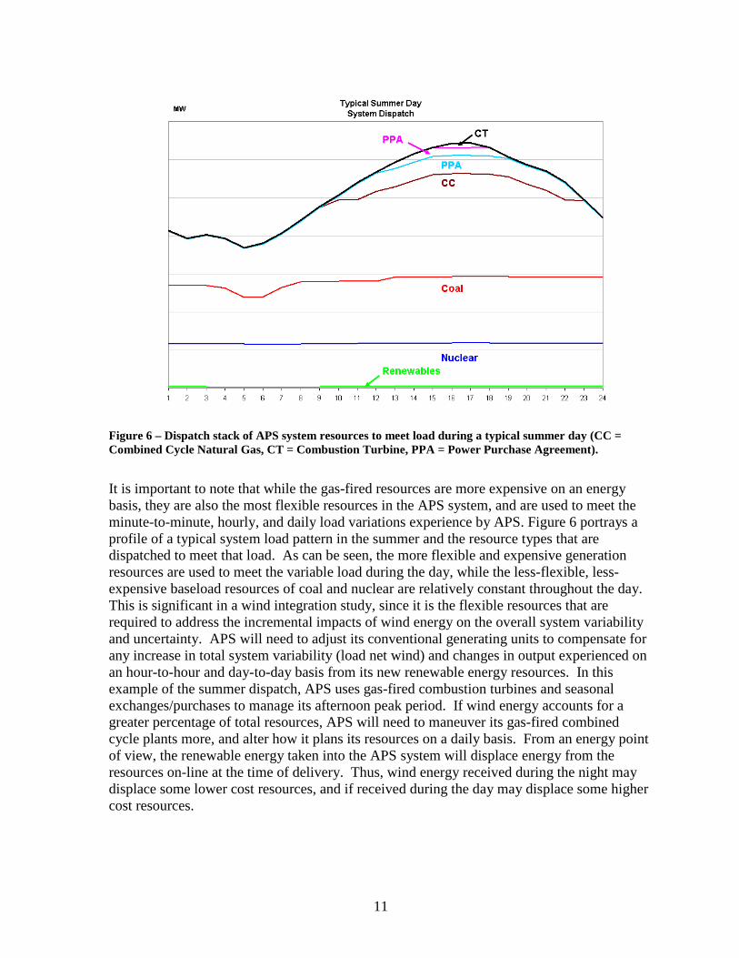
Figure 6 – Dispatch stack of APS system resources to meet load during a typical summer day (CC = Combined Cycle Natural Gas, CT = Combustion Turbine, PPA = Power Purchase Agreement).

It is important to note that while the gas-fired resources are more expensive on an energy basis, they are also the most flexible resources in the APS system, and are used to meet the minute-to-minute, hourly, and daily load variations experience by APS. Figure 6 portrays a profile of a typical system load pattern in the summer and the resource types that are dispatched to meet that load. As can be seen, the more flexible and expensive generation resources are used to meet the variable load during the day, while the less-flexible, less-expensive baseload resources of coal and nuclear are relatively constant throughout the day. This is significant in a wind integration study, since it is the flexible resources that are required to address the incremental impacts of wind energy on the overall system variability and uncertainty. APS will need to adjust its conventional generating units to compensate for any increase in total system variability (load net wind) and changes in output experienced on an hour-to-hour and day-to-day basis from its new renewable energy resources. In this example of the summer dispatch, APS uses gas-fired combustion turbines and seasonal exchanges/purchases to manage its afternoon peak period. If wind energy accounts for a greater percentage of total resources, APS will need to maneuver its gas-fired combined cycle plants more, and alter how it plans its resources on a daily basis. From an energy point of view, the renewable energy taken into the APS system will displace energy from the resources on-line at the time of delivery. Thus, wind energy received during the night may displace some lower cost resources, and if received during the day may displace some higher cost resources.

12

APS SYSTEM IN 2010 Today, APS, like many electric utilities, finds itself planning to add significant amounts of renewable resources in the future. The Arizona Corporation Commission (ACC) approved a new renewable resource requirement which directs APS to supply 15% of its energy needs from renewable resources by the year 2025. APS’ future resource plans include a mix of renewable resources that meet this requirement. Since this study focuses on APS’ 2010 system load and resources to compute an estimate of the integration cost impact, it is important to understand the expected generation resources and load patterns in 2010. Recall, the reason for considering 2010 as the study year is because there is a high level of understanding of what the system resources and load requirements will be, as well as the system operation and market, and thus confidence in the ability to predict the integration impact and cost. Historical load for 2004, coupled with simulated wind generation from 2004, are the base data required for the integration analysis. As such, it was necessary to scale the 2004 hourly loads to the expected energy and peak load in 2010. The scaling was performed by APS’ load forecasting group, and is displayed in the chart shown is Figure 7. As can be seen in this figure, the load patterns experienced in 2004 have been maintained in the 2010 projection, thus preserving the correlation between the load profile and the wind generation profile (derived from the 2004 wind simulation, to be presented in the next section).

0

1,000

2,000

3,000

4,000

5,000

6,000

7,000

8,000

9,000

0 1000 2000 3000 4000 5000 6000 7000 8000

Hour of Year

Load

(M

W)

2010 load data (scaled)

2004 load data

8760

Figure 7 – The hourly load pattern for APS in 2004, scaled to meet the expected 2010 energy requirement and peak load.

13

At its present growth rate, APS expects its peak load to be around 7,900 MW in 2010. APS’ future resource plans address this additional load with a diverse portfolio of resources, including future renewable resources. These renewable resources tend to take the form of long-term contracts between the developer/owner/operator and APS. The contracts are commonly structured such that APS takes the full output of the renewable generation facility, whatever that amount may be for a particular hour or day. Due to the nature of these ‘must-take’ contracts, the dispatch of APS’ conventional resources must be adjusted to accommodate the non-dispatchable renewable resources.

MARKET SETUP AND SYSTEM OPERATION Arizona Public Service Company is an investor owned utility. It is regulated within Arizona by the five member, publicly elected Arizona Corporation Commission, and for interstate transmission and wholesale sales of electricity by the Federal Energy Regulatory Commission (FERC). It is essentially a vertically integrated utility, in that it owns and operates transmission and generation facilities and distributes electricity as a load serving entity. With respect to electric reliability, APS is a member of the Western Electricity Coordinating Council (WECC) which is a region of the North American Electric Reliability Corporation (NERC). APS also participates as a member of the Southwest Reserve Sharing Group (SRSG), which is composed of 15 member organizations that cooperate in a contingency reserve sharing pool “in order to realize a more efficient and economic power system operation while maintaining the reliability of the interconnected system”.iii The contingency reserve requirement for APS at any given moment is that it has set aside reserves equal to 7% of its instantaneous generation from thermal resources (coal, nuclear, gas). For this study, APS assumed 7% reserves were also required for all wind power resources. Of these contingency reserves, one-half must be spinning (on-line, synchronized to the grid, and ready to generate if called upon) and the other half may be non-spinning but must be available within a 10-minute call. APS also maintains “regulating” reserves that are on-line generation resources used to maintain scheduled power flows into and out of the APS control (balancing) area and to maintain system frequency. These resources are what provide the regulation and load following needed to meet its control performance standards (CPS1 and CPS2) via managing the area control error (ACE).5,6,7 As wind energy is a variable resource, it increases the requirements for regulation and load following needed to meet the CPS requirements. Within APS, the combination of contingency and regulating reserves are called “operational reserves.” From a timing perspective, APS makes transactions that are long-term (weeks to months ahead), day(s) ahead, or hour ahead. From a market perspective, APS functions in a bilateral market, meaning that all transactions occur between two trading partners that buy/sell power at some agreed upon price. For day-ahead or long-term transactions, there are typically many potential trading partners; but as for hour ahead, the number of available trading partners is typically less. This differs from other more fully developed markets where there are many participants, both those that sell power to the market and those that purchase. For example, in markets such as those operated by PJM (see www.pjm.com/about/overview.html), the

iii See http://www.srsg.org/, accessed July 2007.

14

Midwest Independent System Operator (MISO; see www.midwestiso.org/home), or the California Independent System Operator (CaliforniaISO; see www.caiso.com/), there are many entities bidding into the market simultaneously to either buy or sell power, and transaction frequently occur within the hour of operation. Furthermore, as the market within which APS participates typically operates with transactions occurring up to the hour of operation, other markets, such as those mentioned above, have sub-hourly transactions. This is significant in the context of wind integration since it is typically less costly to integrate wind with more robust, sub-hourly markets.3 With respect to where APS can transact power purchases/sales, the point-of-delivery can be at many locations on the perimeter of APS’ transmission system (see Figure 8). When a transaction is made, the typical set-up is that the trading partner must deliver (or receive) the power at a particular point on the transmission system and arrange for adequate transmission to get the power to/from that point. Referring to Figure 8, some of the delivery points on the APS system are substations at Mead, Glen Canyon, Four Corners, Navajo, Saguaro, Palo Verde, West Wing, plus some others. Having several places at which transactions can occur increases the number of potential trading partners. In the bilateral market within which APS functions, the dominant form of transaction is purchases/sales of flat blocks of energy. In the southwest, there is no real market for ancillary

Figure 8 – Illustration of the APS high-voltage transmission system.

15

services (e.g., regulation and load following), which is important since these are two ancillary services for which the need increases due to wind integration. As a consequence, these services must be provided by APS using it own resources. Furthermore, all transactions related to providing power or balancing the power system must be made before the hour of operation (i.e., not within the hour, except on an emergency basis), and often the day before operation. From an economic standpoint, while many transactions occur in the day-ahead timeframe, it is not desirable to be in a position where APS “must buy” in the hour-ahead market as this type of purchase can be quite expensive. The implication of this to wind integration is that APS must have available all necessary resources to handle balancing of the system with wind power at the beginning of each hour of operation. In particular, the system planner must make sure there are sufficient regulating and load following resources available during each hour to handle the system variability, including the influence of wind energy. This philosophy also extends to the day-ahead market, since there is no real availability of ancillary services for balancing the system on the market. Therefore, for the purpose of this study, all resources required for load following and regulation were provided by APS system resources (including those available via power purchase agreement (PPA), as indicated in Table 2 and Figure 6). Since APS’ flexible generation resources able to accommodate the system variability are typically expensive to operate (e.g. a combustion turbine), it is beneficial to have a good forecast of the load and a good forecast of the wind energy, so that no more of these resources are employed than necessary. The effect of hour-ahead and day-ahead uncertainty will be discussed in a later section of this report. However, it is worth mentioning here that the uncertainty inherent in a wind energy forecast causes an increased amount of operating reserves to be set aside. The amount of additional reserves set aside decreases as the accuracy of the wind forecast increases. The transactions of importance in this study, i.e., those that relate to the regulation, load following, and unit commitment processes, are the day-ahead and hour-ahead transactions. In the day-ahead time frame, APS will commit units for the following day. This commitment process has three primary objectives: 1) to ensure adequate generation is available to meet the load, 2) to set aside requisite contingency reserves to ensure system reliability, and 3) to ensure there are sufficiently flexible resources available to follow variations in the load (i.e., regulating reserves) and thus satisfy NERC control performance standards. This process of unit commitment is carried out using an algorithm that will economically optimize performance. This requires forecast information of the system load throughout the day, its variability (need for regulation and load following), the availability of its generation resources and their characteristics (heat rates, ramp rates, start-up times, etc.), and information about the resources/prices available or sought on the market. When wind energy is integrated into utility operations, a forecast of wind energy and its expected variability is also required. As will be demonstrated later, a high quality wind energy forecast is beneficial to keeping down wind integration costs. Transactions related to day ahead planning are generally completed by 6 a.m. the day prior to operation. Within the day of operation, the load, generation resources, and market conditions are better known than during the day-ahead commitment process. Thus, APS will make transactions up to the hour ahead of operation, re-optimizing economical use of system resources and scheduling them for use. While these transactions often occur one-half hour prior to the hour

16

of operation, they can occur anytime up to about 10-minutes before the hour. Within the hour, some of the system resources are specifically devoted to regulating reserves. These resources can rapidly respond to variations in load (or load net wind), and follow the ramps from hour to hour. Some of the regulating reserves are operated on Automatic Generation Control (AGC), and therefore can respond quickly to changes in load (or load net wind), thus keeping the system in balance (a “non-economic” dispatch to maintain system frequency and interchange schedules).

ROLE OF TRANSMISSION IN STUDY Since the purpose of this study is to determine the cost of integrating wind energy due to its variability and uncertainty, it is not necessary to account for the transmission necessary to bring the wind energy to the APS grid. At the heart of this integration cost study (and many others) is a comparison between the operating costs of the system incorporating wind energy with the system incorporating some “baseline” energy resource that does not possess the wind’s variability and uncertainty. Thus, the cost of the transmission “washes out” and does not factor into the integration cost, as it would be the same in each scenario. Further, developing a wind power plant requires a combination of a good wind resource, access to land, and access to transmission, all of which take significant time and understanding to accurately define, and which will not substantially alter the results. The approach adopted in this study has been to rationally locate hypothetical wind power plants at diverse geographic locations, sufficient to allow flexibility in modeling the integration impacts and thus determine a realistic value for the integration cost. As will be explained in the following section, no preliminary screening of nearby available transmission capacity was made in citing the wind power plants. If the hypothetical plants modeled for this study were actually constructed, some additional transmission capacity would no doubt be required.

17

III. ARIZONA WIND RESOURCE MODELING AND RESULTS An important aspect of any wind integration study is correctly capturing the correlation that exists between wind, load, and weather. In particular, it is essential that the wind and load data be time-synchronized in simulating the utility system planning and operation. This permits the simulation, within the limitations inherent in any system model, to accurately characterize the impact of the wind on system operation and costs. Thus a key component of this project was to accurately model proposed wind power production that could contribute toward the APS generation mix, for which the integration cost could then be determined. The wind power plants modeled need not be in the exact location nor have the same output as actual wind plants that may be built in the Arizona. Rather, the purpose here is to generate wind power plant output profiles that are typical of what could occur, and located in areas within Arizona where they might be built based upon the available wind resource. Consequently, the results of the integration cost study should be considered as simply being representative of potential Arizona wind resource development. In producing the wind energy simulation, NAU and APS collaborated with the Arizona Power Authority (APA), which is the organization within Arizona responsible for receiving and distributing power from Hoover dam and powerplant, and is also conducting a wind energy study. Both APS and APA, working with NAU, contracted with 3TIER, a company that specializes in renewable energy modeling and forecasting, to perform the wind energy “backcast” and power prediction. NAU was responsible for defining the wind modeling input parameters, determining the wind power plant locations and layouts, and then synthesizing the wind power production model output into coherent wind power scenarios for input to the APS power system simulation. A description of the wind modeling and its results are presented in the subsections listed below:

• Wind Model Set-up and Requirements • Meso-Scale Wind Modeling • Results of the Meso-Scale Wind Model • Wind Power Plant Modeling • Results of Wind Power Modeling

WIND MODEL SET-UP AND REQUIREMENTS

There are two basic requirements of a wind energy model as used in a wind integration study: 1) it be physics-based and of sufficient resolution in both time and space to accomplish the goals of the integration study; and 2) it accurately convert wind speed information to wind power production data, including correctly characterizing the variability exhibited by the wind power plants. As to this later point, because the wind speed and direction varies even over small areas, no two wind turbines see the same input wind speed nor have identical power output. Further, each wind turbine possesses a significant amount of inertia, hence its output cannot respond to the faster fluctuations of the wind speed. For these reasons, one

18

cannot simply take the output of a meso-scale wind model (or wind anemometer data) and run it directly through a manufacturer’s turbine power curve to accurately estimate a power output for an entire wind power plant. There must be some method to ensure the variability of modeled wind plant output emulates the output that actually realized in operational wind power plants. Given these considerations, the following parameters were defined for the wind modeling in consultation with the project technical advisory group:

• Wind speeds were simulated with 3TIER’s meso-scale model throughout the zones shown in Figure 9, for the historical years 1996 to 2006, with a focus on 2003, 2004, and 2005.

• The East (APSCo) and West (APA) zones demarked by the blue and red boxes in Figure 9 were both modeled using a grid spacing of 5-km (the meso-scale model predicts wind speed, direction, air density, etc., at pre-defined grid points), for the historical period 1996 to 2006.

• Two smaller zones, identified by the small black rectangles in Figure 9, were selected for additional higher-resolution modeling with 1-km grid spacing. These zones are the Aubrey Cliffs, north of Seligman, and Gray Mountain, west of Cameron, and are known to have good potential for wind resource development, but also have highly variable topography. Because a 5-km resolution simulation may not adequately capture the effects of the topographical features present in these areas, more refined 1-km resolution simulations were conducted. The higher resolution zones were modeled only for historical years 2003, 2004, and 2005.

• The time-step of the meso-scale simulation was 10-minutes (for all zones). This resolution in time allows study of the intra-hour wind variations, and can easily be modified for an hourly power system simulation.

• Wind speed and related meteorological parameters were predicted at 50-m, 80-m, and 100-m above the ground at each model grid point.

• For the wind power modeling, power curves for a GE 1.5 MW wind turbine was used, employing a 77-m rotor diameter, an 80-m hub height, and with adjustment for the local air density at each proposed site.

5 km Grid

1 km Grid

West Zone

East Zone

5 km Grid

1 km Grid

West Zone

East Zone Figure 9 – Specific modeling zones for the meso-scale wind energy simulation.

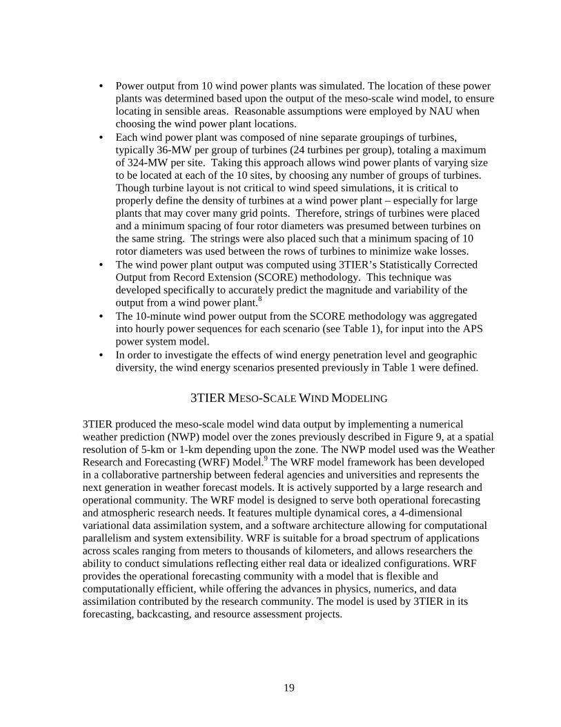
19

• Power output from 10 wind power plants was simulated. The location of these power

plants was determined based upon the output of the meso-scale wind model, to ensure locating in sensible areas. Reasonable assumptions were employed by NAU when choosing the wind power plant locations.

• Each wind power plant was composed of nine separate groupings of turbines, typically 36-MW per group of turbines (24 turbines per group), totaling a maximum of 324-MW per site. Taking this approach allows wind power plants of varying size to be located at each of the 10 sites, by choosing any number of groups of turbines. Though turbine layout is not critical to wind speed simulations, it is critical to properly define the density of turbines at a wind power plant – especially for large plants that may cover many grid points. Therefore, strings of turbines were placed and a minimum spacing of four rotor diameters was presumed between turbines on the same string. The strings were also placed such that a minimum spacing of 10 rotor diameters was used between the rows of turbines to minimize wake losses.

• The wind power plant output was computed using 3TIER’s Statistically Corrected Output from Record Extension (SCORE) methodology. This technique was developed specifically to accurately predict the magnitude and variability of the output from a wind power plant.8

• The 10-minute wind power output from the SCORE methodology was aggregated into hourly power sequences for each scenario (see Table 1), for input into the APS power system model.

• In order to investigate the effects of wind energy penetration level and geographic diversity, the wind energy scenarios presented previously in Table 1 were defined.

3TIER MESO-SCALE WIND MODELING

3TIER produced the meso-scale model wind data output by implementing a numerical weather prediction (NWP) model over the zones previously described in Figure 9, at a spatial resolution of 5-km or 1-km depending upon the zone. The NWP model used was the Weather Research and Forecasting (WRF) Model.9 The WRF model framework has been developed in a collaborative partnership between federal agencies and universities and represents the next generation in weather forecast models. It is actively supported by a large research and operational community. The WRF model is designed to serve both operational forecasting and atmospheric research needs. It features multiple dynamical cores, a 4-dimensional variational data assimilation system, and a software architecture allowing for computational parallelism and system extensibility. WRF is suitable for a broad spectrum of applications across scales ranging from meters to thousands of kilometers, and allows researchers the ability to conduct simulations reflecting either real data or idealized configurations. WRF provides the operational forecasting community with a model that is flexible and computationally efficient, while offering the advances in physics, numerics, and data assimilation contributed by the research community. The model is used by 3TIER in its forecasting, backcasting, and resource assessment projects.

20

Input Data The main input data for wind energy backcast simulations are historic global weather archives, which are maintained by operational weather forecasting centers around the world including the United States National Center for Environmental Prediction (NCEP). These global archives represent the overall state of the atmosphere over the entire planet and are themselves the result of a sophisticated computer “reanalysis” of available surface and upper air observations, combining tens of thousands of individual measurements around the globe into a consistent physical state.iv The analysis scheme is a 3-dimensional variational scheme cast in spectral space. The assimilated observations are:

a. Upper air rawinsonde observations of temperature, horizontal wind and specific humidity

b. Operational TOVS vertical temperature soundings from NOAA polar orbiters

c. Cloud tracked winds from geostationary satellites

d. Aircraft observations of wind and temperature

e. Land surface reports of surface pressure

f. Oceanic reports of surface pressure temperature, horizontal wind and specific humidity.

Due to the necessity to represent the entire globe, the NCEP/NCAR reanalysis data set is maintained at a relatively coarse horizontal resolution and, by itself, does not contain the level of detail necessary to resolve the wind flow patterns over smaller geographic regions or over a single project. However, these data do provide a good representation of the history of large-scale spatial patterns in the atmosphere (i.e., the position of high and low pressure systems; the location of the jet stream) as well as the general state of the ocean (e.g., sea surface temperatures) and land surface condition (e.g., soil moistures). 3TIER maintains an archive of 40+ years of global weather data from NCEP. Combining these coarse data with high-resolution land-use data and a high-resolution numerical weather simulation model allows regional and site specific wind fields to be accurately reconstructed.

To accurately resolve the regional wind fields requires an ability to model the interaction of large scale weather systems with the varied terrain, land-use and vegetation of the region. An accurate representation of the local terrain is also important for resolving thermally driven circulations caused by differential heating and cooling of the land surface. 3TIER has customized the WRF model to ingest both the U.S. Geological Survey (USGS) GTOPO30 dataset,v which provides a global 30-second (roughly 900 m) digital representation of land surface topography, as well as higher-resolution 90-meter terrain datasets such as those available from the Shuttle Radar Topography Mission. In addition, WRF employs a 30-second global 24-category land use map (USGS), a 5-min soil texture (FAO) and a 0.15-degree monthly climatology green vegetation fraction. These data sets were used to describe the height and roughness of the earth’s surface for the period of simulation.vi

Model Simulations and Output Variables The WRF model was implemented for the modeling zones using nested domains of

iv Available online at www.cpc.ncep.noaa.gov/products/wesley/reanalysis.html v Available online at http://edc.usgs.gov/products/elevation/gtopo30/gtopo30.html vi Information available at http://srtm.usgs.gov

21

progressively higher spatial grid resolutions of 45-, 15-, and 5-km from the outermost to the innermost domain. The innermost of these domains is the actual zone being modeled. The outer domains are buffer zones, which are extensions of the modeling zone in each direction, included to avoid grid edge effects. The nested grid configuration for the East zone is shown in Figure 10. A similar buffer zone was applied to the high resolution zones (Aubrey Cliffs and Gray Mountain), but the innermost domain was further downscaled to 1-km resolution. Output from the simulation was a three dimensional data set of the state of the atmosphere over the entire study area at a temporal resolution of ten minutes and a spatial resolution of 5-km (1-km for the high resolution areas). These data include all static and meteorological variables required to calculate wind energy output above the earth’s surface, including wind speed and wind direction, the temperature of the ground surface, the air temperature, the specific humidity, the air pressure, incoming longwave radiation, incoming shortwave radiation and precipitation at the ground surface. Evaluation of Model Output 3TIER’s analysis of model output focused on two aspects of the modeled wind fields: internal consistency and comparison with observation. The first evaluation simply determines whether the modeled fields are subject to numerical instabilities and the like, which are directly related to model setup and implementation. All model output was subjected to quantitative controls of numerical stability based on Courant limits; visual inspection of wind speed fields focusing on detection of instabilities and/or spurious standing waves; and a

Figure 10 – Map with the nested model domain used in the simulation of the East zone. The innermost black box denotes the requested study area (simulated at a 5 km horizontal resolution, as shown by the black dots).

22

qualitative analysis of the wind distribution at each grid point. The second evaluation relies on the availability of observations with which to compare the model simulations. In general, 3TIER analyzes model output by comparing it to data collected in the domain during time periods that overlap with the simulations. This includes a comparison of modeled and observed means, variances, diurnal distributions, and Weibull parameters, as well as correlation statistics computed on hourly, daily, and monthly time scales.

RESULTS OF MESO-SCALE WIND MODEL Maps displaying the results of the meso-scale wind simulation for the West and East modeling zones are displayed in Figure 11 and Figure 12. Each map displays the wind power density (W/m2) at 80 meters above the ground since it is more directly indicative of the wind energy potential at a given site and thus better suited to guide selecting wind power plant locations. The wind power density indicated at any point on this map represents the value at that location averaged over the eleven year period of the simulation. Each figure includes a color scale indicating the wind power density and wind power classification (1, 2, etc.). For reference, a class 3 wind resource is defined as between 300 and 400 W/m2 which corresponds to the light orange coloring on the map; class 4 wind resource is defined as between 400 and 500 W/m2; etc. The wind class designations shown on the scale correspond to the mid-point of the wind class. Since class 3 is considered the minimum wind class that currently can support an economically feasible wind power plant, the areas where potential

Figure 11 – Wind power density map of the West (APA) modeling zone.

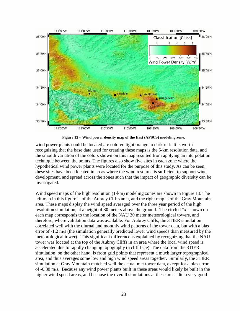
23

Figure 12 – Wind power density map of the East (APSCo) modeling zone.

wind power plants could be located are colored light orange to dark red. It is worth recognizing that the base data used for creating these maps is the 5-km resolution data, and the smooth variation of the colors shown on this map resulted from applying an interpolation technique between the points. The figures also show five sites in each zone where the hypothetical wind power plants were located for the purpose of this study. As can be seen, these sites have been located in areas where the wind resource is sufficient to support wind development, and spread across the zones such that the impact of geographic diversity can be investigated. Wind speed maps of the high resolution (1-km) modeling zones are shown in Figure 13. The left map in this figure is of the Aubrey Cliffs area, and the right map is of the Gray Mountain area. These maps display the wind speed averaged over the three year period of the high resolution simulation, at a height of 80 meters above the ground. The circled “x” shown on each map corresponds to the location of the NAU 30 meter meteorological towers, and therefore, where validation data was available. For Aubrey Cliffs, the 3TIER simulation correlated well with the diurnal and monthly wind patterns of the tower data, but with a bias error of -1.2 m/s (the simulation generally predicted lower wind speeds than measured by the meteorological tower). This significant difference is explained by recognizing that the NAU tower was located at the top of the Aubrey Cliffs in an area where the local wind speed is accelerated due to rapidly changing topography (a cliff face). The data from the 3TIER simulation, on the other hand, is from grid points that represent a much larger topographical area, and thus averages some low and high wind speed areas together. Similarly, the 3TIER simulation at Gray Mountain matched well the actual met tower data, except for a bias error of -0.88 m/s. Because any wind power plants built in these areas would likely be built in the higher wind speed areas, and because the overall simulations at these areas did a very good

24

Figure 13 – Wind speed maps of the two high resolution modeling zones: Aubrey Cliff (left) and Gray Mountain (right).

job matching the met tower data except for the bias error, the decision was made to apply a bias error correction to all data points in each of these zones. The bias adjusted wind speeds were used in the wind power modeling at these two sites.

WIND POWER PLANT MODELING For the purpose of modeling output from the proposed wind power plants an approach known as the “Statistically Corrected Output from Record Extension” (SCORE). This methodology was developed at 3TIER. One motivation behind this technique is that power output from a wind turbine does not precisely match that which would be predicted by actual wind speed run through the turbine power curve. An example power curve from a wind turbine in an operating power plant is shown in Figure 14. As can be seen, the observations of wind power versus wind speed spread around the turbine power curve forming a thick band. The reasons for this spread of observations are many related to turbine inertia, changes in the wind speed, direction, etc., but it is a commonly observed behavior and can be modeled statistically. Another motivation for the SCORE method is that the 10-minute wind speed record from an NWP model tends to be smoother than that observed on-site. Thus taking the output from an NWP model and running it directly through a turbine power curve, while able to predict the mean power output well, will not correctly reproduce the variability in the 10-minute, or even hourly, timeframe. For these reasons, the SCORE methodology was developed with the explicit intention of correcting the wind power output predicted via an NWP model and turbine power curve, by interjecting the appropriate amount of variability. SCORE is based upon statistical relationships obtained from turbine level wind speed and corresponding turbine power observations from actual wind power plants, combined with NWP modeling of the wind speed at these plants. These statistics were used to develop a probabilistic model, implemented using probability density functions (PDFs), to reproduce hourly and ten-minute variations of power output. The model accounts for the locations of the turbines within the region simulated by the NWP model and therefore captures the effect

25

Figure 14 – Example power curve from a wind turbine operating in a wind power plant (source: 3TIER).

of geographic diversity on the turbine power outputs directly. Finally, the probabilistic model is used to statistically correct the power output values based on the NWP modeled record extension. After applying this correction, the resulting power output sequence from each turbine has been adjusted such that it exhibits the variability (both 10-minute and hourly) similar to that observed at operational wind power plants. Implicit in this method is the assumption that the wind power plants being modeled will exhibit similar variability characteristics as the power plants from which the statistical correction was developed. 3TIER’s experience with SCORE suggests that this is a reasonable assumption. When applying the SCORE methodology, a number of parameters were required to condition the model for operations. Since this is an investigative study using hypothetical wind power plants, suitable assumptions were made about the wind power plants and applied consistently to all ten power plants being modeled. The following inputs were provided to the SCORE model:

1. Ten-minute resolution wind speed data time-series at all grid points from the NWP model. The output from the ten-minute temporal resolution NWP modeling, at 5-km spatial resolution for all wind power plants except for the two located in the 1-km resolution modeling zones at Aubrey Cliffs and Gray Mountain.

2. The total capacity of each wind power plant, and the turbine groupings that make up the power plant. Table 3 shows the total capacity and size of turbine groupings at each of the ten hypothetical wind power plants at the locations shown in Figure 11 and Figure 12.

26

3. The type of turbine in the study: GE 1.5sle turbine with a 77 m rotor.vii a. Hub height of the turbines in the study: 80 meter. b. The manufacturer’s rating curve with a reference air density.

4. Turbine locations within each wind power plant.

With respect to defining the turbine locations within each wind power plant, NAU considered the topography and prevailing wind direction at each site, and defined a reasonable layout for the wind turbines. Minimum spacing criteria between the turbines of four rotor blade diameters between adjacent turbines, and ten rotor diameters between rows of turbines were assumed. Figure 15 shows an example of how the turbine groupings were laid out at the Bullhead City site. Note the prevailing wind direction is south/north at Bullhead City, therefore the turbine groups are laid out in strings perpendicular to this direction. The horizontal lines shown on the topographical map (right side) correspond to the turbine strings (a row of turbines). At this particular site, there were five groupings of 26 turbines each; therefore one turbine group is composed of the turbines set along two adjacent horizontal lines. The locations of the end points of each turbine string was provided by NAU to 3TIER, who then determined the location of the turbines along each string using the adjacent spacing criterion. Once the turbine locations were defined, each turbine was associated to the wind speed simulation at one of the NWP grid points. An example of how turbines within a wind power plant are associated with NWP grid points is shown in Figure 16. With all the model parameters defined, the actual implementation of the SCORE method is similar to a Monte Carlo approach. First, the appropriate wind speed and grid point locations are extracted from the NWP files. Then, the links between each turbine and the nearest grid point are established. At this stage, the wind speeds from the NWP model have yet to be

Table 3 – Listing of the total installed nameplate capacity of wind turbines at each wind power plant.

vii The turbine type and hub height are considered to be of lower-order influence in a utility wind integration study, as it is the wind resource and the challenge in predicting it that are responsible for the variability and uncertainty that drive operating cost impacts.

Wind Power Plant Sites (West/APA Zone)

Nameplate Capacity*

[MW]

Wind Power Plant Sites (East/APSCo Zone)

Nameplate Capacity*

[MW] Anderson 324 Greer 324

Aubrey Cliffs 324 Hay Hollow 324 Bullhead 195 Pinedale 324

Cottonwood 333 Springerville 324 Gray Mountain 324 Young 324

Total West 1,500 Total East 1,620 * Note, all wind power plants were composed of nine groupings of 24 turbines (36 MW per group), except for Bullhead (five groups, 26 turbines/group equaling 39 MW per group) and Cottonwood (seven groups with 24 turbines/group, one group with 26 turbines, and one with 28 turbines equaling 42 MW).

27

Figure 15 – Turbine layout at the hypothetical wind power plant located near Bullhead City.

converted to power output. The remaining steps in the SCORE technique are as follows:

1. Calculate the hourly time series from the NWP model simulations based on the 10-minute NWP output.

2. For each NWP model grid point, convert the hourly wind speed time-series into an hourly power output time-series using the manufacturer’s power curve, corrected for the local air density.

3. For each turbine, locate the nearest grid point and apply the PDFs (created from hourly variations) to convert the theoretical power output at the grid point into probabilistic power output from the turbine.

After this operation, the time-series from the NWP record extension has been statistically

Figure 16 - Example of turbine layout from a wind power plant, showing the links to the nearest NWP points: turbines are red, NWP points are blue and links are green. In the turbine layout shown here (not from the current study), the turbine locations were not set along straight lines.

57

58

59

60

61

62

63

64

65

66

57

58

59

60

61

62

63

64

65

66

57

58

59

60

61

62

63

64

65

66

3TIER Wind Map Aerial Image Topo Map with Turbine Layout

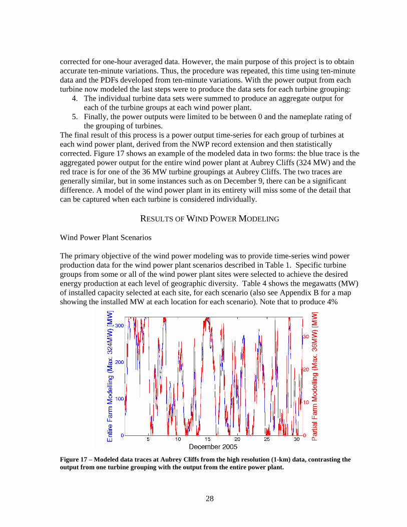
28

corrected for one-hour averaged data. However, the main purpose of this project is to obtain accurate ten-minute variations. Thus, the procedure was repeated, this time using ten-minute data and the PDFs developed from ten-minute variations. With the power output from each turbine now modeled the last steps were to produce the data sets for each turbine grouping:

4. The individual turbine data sets were summed to produce an aggregate output for each of the turbine groups at each wind power plant.

5. Finally, the power outputs were limited to be between 0 and the nameplate rating of the grouping of turbines.

The final result of this process is a power output time-series for each group of turbines at each wind power plant, derived from the NWP record extension and then statistically corrected. Figure 17 shows an example of the modeled data in two forms: the blue trace is the aggregated power output for the entire wind power plant at Aubrey Cliffs (324 MW) and the red trace is for one of the 36 MW turbine groupings at Aubrey Cliffs. The two traces are generally similar, but in some instances such as on December 9, there can be a significant difference. A model of the wind power plant in its entirety will miss some of the detail that can be captured when each turbine is considered individually.

RESULTS OF WIND POWER MODELING Wind Power Plant Scenarios The primary objective of the wind power modeling was to provide time-series wind power production data for the wind power plant scenarios described in Table 1. Specific turbine groups from some or all of the wind power plant sites were selected to achieve the desired energy production at each level of geographic diversity. Table 4 shows the megawatts (MW) of installed capacity selected at each site, for each scenario (also see Appendix B for a map showing the installed MW at each location for each scenario). Note that to produce 4%

Figure 17 – Modeled data traces at Aubrey Cliffs from the high resolution (1-km) data, contrasting the output from one turbine grouping with the output fr om the entire power plant.

29

Table 4 – Megawatts (MW) of installed capacity from each site employed in the various scenarios considered.

MW of Installed CapacityWind Energy: 1% 4% 4% 4% 10%

Modeling Zone Site \ Diversty: Med High Med Low MedWest / APA Bullhead City 78

Cottonwood Cliffs 36Aubrey Cliffs 36 72 144 324Gray Mountain 72 36 180 288 324Anderson 72 144 180 324

East / APSCo Young 36 288Pinedale 36Hay Hollow 36Greer 72Springerville 36

Total 108 510 468 468 1260 of APS’s annual energy in 2010, it took 468 MW of wind power for the medium and low diversity cases, but 510 MW in the high diversity case. The reason for this is that some turbine groups from higher producing sites (e.g., Gray Mountain and Aubrey Cliffs) were replaced with turbine groups from lower producing sites (e.g., Springerville, Hay Hollow, etc.), requiring more wind power capacity to produce the same amount of wind energy. Note when selecting turbine groups for a given scenario (1%, 4%, or 10%), it was necessary to select whole groups of turbines. Since the groups of turbines were created in multiples of 36 MW, in some cases it was not possible to combine the turbine groups to yield the precise amount of energy sought. Table 5 summarizes some key statistics for each scenario, including the actual amount of wind energy produced as a percentage of APS 2010 energy.

Table 5 – Summary of some key wind power statistics for the wind penetration and geographic diversity cases considered.

Scenario Statistics

% Wind by Energy

% Wind by power

Geographic Diversity

Ave 2003-2005 capacity

factor for case

Nameplate Capacity of

Wind Turbines

(MW)

Actual % of APS 2010

Energy

1 1.4% Med 36.7% 108 1.00%4 6.5% High 31.0% 510 4.00%4 5.9% Med 33.8% 468 4.00%4 5.9% Low 33.5% 468 3.97%10 15.9% Med 32.6% 1260 10.38%

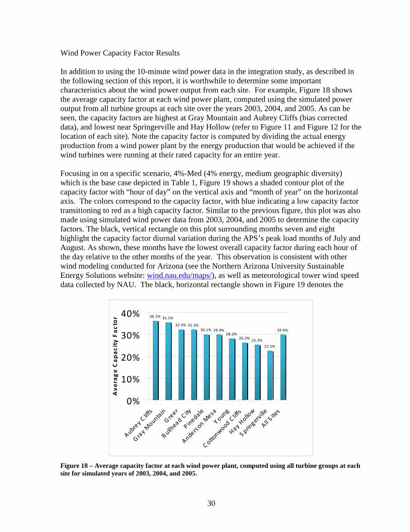
30

Wind Power Capacity Factor Results In addition to using the 10-minute wind power data in the integration study, as described in the following section of this report, it is worthwhile to determine some important characteristics about the wind power output from each site. For example, Figure 18 shows the average capacity factor at each wind power plant, computed using the simulated power output from all turbine groups at each site over the years 2003, 2004, and 2005. As can be seen, the capacity factors are highest at Gray Mountain and Aubrey Cliffs (bias corrected data), and lowest near Springerville and Hay Hollow (refer to Figure 11 and Figure 12 for the location of each site). Note the capacity factor is computed by dividing the actual energy production from a wind power plant by the energy production that would be achieved if the wind turbines were running at their rated capacity for an entire year. Focusing in on a specific scenario, 4%-Med (4% energy, medium geographic diversity) which is the base case depicted in Table 1, Figure 19 shows a shaded contour plot of the capacity factor with “hour of day” on the vertical axis and “month of year” on the horizontal axis. The colors correspond to the capacity factor, with blue indicating a low capacity factor transitioning to red as a high capacity factor. Similar to the previous figure, this plot was also made using simulated wind power data from 2003, 2004, and 2005 to determine the capacity factors. The black, vertical rectangle on this plot surrounding months seven and eight highlight the capacity factor diurnal variation during the APS’s peak load months of July and August. As shown, these months have the lowest overall capacity factor during each hour of the day relative to the other months of the year. This observation is consistent with other wind modeling conducted for Arizona (see the Northern Arizona University Sustainable Energy Solutions website: wind.nau.edu/maps/), as well as meteorological tower wind speed data collected by NAU. The black, horizontal rectangle shown in Figure 19 denotes the

36.2% 35.5%

32.4% 32.3%30.1% 29.9%

28.2%26.3%

25.2%

22.5%

29.9%

0%

10%

20%

30%

40%

Aubre

y Clif

fs

Gra

y Mounta

in

Gre

er

Bullh

ead City

Pin

edale

Anders

on Mesa

Young

Cotto

nwood C

liffs

Hay H

ollow

Sprin

gervill

e

All

Site

s

Av

era

ge

Ca

pa

cit

y F

ac

tor

Figure 18 – Average capacity factor at each wind power plant, computed using all turbine groups at each site for simulated years of 2003, 2004, and 2005.

31

HOUROF

DAY

Month of Year

Capacity Factor Color Scale

HOUROF

DAY

Month of Year

Capacity Factor Color Scale

Figure 19 – Shaded contour plot of the capacity factor for scenario 4%-Med (4% wind energy and medium geographic diversity), showing how the capacity factor varies with hour of day and month of year.

capacity factor variation throughout the year during the peak load hours of the afternoon (3 p.m. to 8 p.m.). As indicated, generally the highest capacity factors that occur during the day happen in the afternoon during the peak load hours. With respect to the other wind scenarios considered (see Table 4), their seasonal and diurnal capacity factor variations are depicted in Figure 20. Consistent with the information presented in Figure 19, with respect to helping meet the peak load, the seasonal availability of the wind power is not advantageous, while the diurnal variation is. Milligan has suggested

0%

5%

10%

15%

20%

25%

30%

35%

40%

45%

50%

1 2 3 4 5 6 7 8 9 10 11 12 13 14 15 16 17 18 19 20 21 22 23 24

Hour of Day

Cap

acity

Fac

tor

4%-High4%-Med4%-Low

0%

5%

10%

15%

20%

25%

30%

35%

40%

45%

50%

Jan Feb Mar Apr May Jun Jul Aug Sep Oct Nov Dec

Month of Year

Cap

acity

Fac

tor

4%-High4%-Med4%-Low

Figure 20 – Diurnal and seasonal capacity factor variations for the low, medium, and high geographic diversity cases for 4% wind energy penetration.

32

a method to approximate the capacity value of the wind power that may be counted upon to meet peak load. 10,11 While this method is not a substitute for utility techniques of computing the Effective Load Carrying Capability (ELCC) of a generator, it has been shown to provide a fair indication of the wind’s capacity value, within a few percent. The basic idea of this technique is to compute the average capacity factor during the highest 10% of load hours during the year. Taking this value of the capacity factor and multiplying by the nameplate capacity then provides an approximation of the capacity value from the wind power plant. Figure 21 shows a plot of the average capacity factor during the highest 10% of load hours during 2003, 2004, and 2005, for the base case wind scenario of 4% wind energy penetration and medium geographic diversity (4%-Med). Also shown is the average capacity factor for 100% of the load hours (the entire year). Two points of interest emerge from this plot: 1) the capacity value will be less than the average capacity factor for the entire year, reflective of the lower wind energy production during the peak summer months; and 2) the wind power will have a capacity value that is a significant fraction of its average capacity factor, due to the afternoon peaking nature of the wind. Note that this type of estimate is not a substitute for an ELCC calculation, but is only an approximation. Furthermore, only three years are plotted in Figure 21 using simulated wind data, whereas it would be necessary to use actual wind data and advisable to use several years of data in determining the ELCC. That said, wind power generally does not vary in output more that about 15% from year to year, as demonstrated by Westrick12 in the Pacific Northwest, thus it is likely that an Arizona wind resource will contribute some amount of capacity toward the system peak. Wind Power Ramping Analysis The variability of wind power output for large-scale wind power penetration creates a challenge for power system and transmission network operators. The variable wind power

0%

5%

10%

15%

20%

25%

30%

35%

40%

2003 2004 2005

Year

Mea

n ca

paci

ty fa

ctor

Highest 10% of Load Hours

100% of Load Hours

Figure 21 – Average capacity factor for wind scenario 4%-Med, during APS’s expected highest 10% of load hours during 2010, and for all hours of 2010.

33

must be incorporated into a system that has been optimized for fully schedulable conventional power plants. Therefore, measuring and understanding the extent of the variation that will be introduced to the system through rapid wind power ramping events is crucial for the reliable operation of the power system. Using simulated wind power data from this project, it is possible to quantify the frequency of ramp events of a given size and determine the effect of the size and location of the wind power plant on this frequency. More importantly, the analysis will look at the effect of region-wide smoothing on two time-scales for both zones modeled: West (APA) and East (APS). For the purposes of this ramping study, each modeled wind power plant was considered in full, rather than the ~36MW sub-groupings, using the full 578,880 data points for each power plant (including the 31st of December 1995 and 1st of January, 2007). While the 5-km resolution data was used for most of this analysis, the bias-corrected, high-resolution (1 km) data, which is considered more accurate than non bias-corrected data, was utilized for the ramping analysis at the Gray Mountain and Aubrey Cliffs wind power plants for the years available: 2003, 2004 and 2005. 10-Minute Ramping Analysis The basic unit of data in this study was wind power averaged over a ten-minute period, derived from the NWP modeling and produced via the SCORE technique. A ten-minute ramp is defined here as the change in power output from one ten-minute time period to the next. Table 6 summarizes 10-minute ramps experienced by each of the ten wind power plants modeled, and in aggregate for each modeling zone (combined output of all wind power plants in each modeling zone). For any given wind power plant, approximately 70-80% of the wind power ramps are less than 2% of the rated capacity. Of the remaining ramps, most are in the 2% to 10% of rated capacity range, with less than 1% of the ramps exceeding 10% of rated capacity. The effect of geographic diversity on the 10-minute ramps is demonstrated

Table 6 – Distribution of ten-minute ramps, sorted by wind power plant and grouped in percentages of rated capacity.

Ramps outside the ±10% of rated capacity range

Ramps in ±2% to ±10% of rated capacity range

Ramps inside the ±2% of rated capacity range

Wind Power Plant

Count % Count % Count %

Anderson 3,568 0.62 112,259 19.39 463,053 79.99 Aubrey Cliffs 4,112 0.71 176,923 30.56 397,845 68.73 Bullhead 4,372 0.76 120,973 20.90 453,535 78.35 Cottonwood 3,444 0.60 115,433 19.94 460,003 79.46 Gray Mountain 5,119 0.89 155,607 26.88 418,154 72.24

Wes

t/A

PA

Zo

ne

Combined Output 223 0.04 59,485 10.28 519,172 89.69 Greer 1,996 0.34 100,939 17.44 475,945 82.22 Hay 4,902 0.85 113,222 19.56 460,756 79.59 Pinedale 3,344 0.58 116,744 20.17 458,792 79.26 Springerville 5,040 0.87 135,932 23.48 437,908 75.65 Young 2,222 0.38 114,930 19.85 461,728 79.76

Eas

t/AP

S Z

on

e

Combined Output 298 0.04 63,750 11.01 514,832 88.94

34

by the ramp statistics for the combined output of the wind power plants in the West/APA and East/APS zones. For the combined output, approximately 90% of the ramps are less that 2% of rated capacity, 10% are in the 2% to 10% range, and 0.04% of the ramps are greater than 10% of rated capacity. The basic reason for this reduction is that the wind fluctuations that cause the 10-minute ramps only have a very small correlation from site-to-site.13 Though the vast majority of ramping events at the 10-minute level are of a magnitude less than 10% of the rated capacity, when operating a utility system it is these infrequent, larger-scale events that must be planned for to ensure reliable operation. A closer look at the 10-minute ramping events greater than 10% of rated capacity is shown in Figure 22 and Figure 23, for the West/APA and East/APS zones respectively. The vertical axis in each of these figures indicates the count of the ramp events of a given magnitude, and the horizontal axis shows histogram bins representing ramp events of a given magnitude, in terms of percentage of nameplate capacity for each wind power plant. The actual values can be found in the table at the bottom of the figure. These two figures show a preponderance of the high magnitude ramp events occur between –20% and +20% of the nameplate capacity. It can also be seen that it is not unusual for a wind power plant to experience ramps of ±40% of the nameplate capacity approximately once a year (note that these histograms show total ramp counts for an 11-year period). Also, the histograms for all sites are skewed to the right, meaning positive ramps outnumber negative ramps. When the wind power plants are combined (shown by the black bars and the bottom rows of the tables) the large magnitude ramps become dramatically less frequent, emphasizing the beneficial effect of geographic diversity. The following conclusions can be drawn from the 10-minute ramping analysis:

• The vast majority of 10-minute ramping events are less than 10% of the wind power plant capacity.

• Although the sizes of the wind power plants are similar, with the exception of Bullhead and Cottonwood (see Table 3), localized weather patterns exist that affect the ramping behavior of the sites such that the ramps at the ten-minute timescale are effectively uncorrelated between the sites.

• The combined output from all wind power plants for the West/APA region and the East/APS region is considerably smoother than any of the individual power plants.

• For all power plants at the ten-minute timescale, the chance of a positive ramp is greater than the chance of a negative ramp. This is useful to know if ramp rate limiting is employed, since it will only work on the up-ramps.

Comparison of 5-km and 1-km Resolution Ten-Minute Data Anemometer data was used to develop a bias-corrected wind power series for each of the wind power plants modeled at the higher spatial resolution of 1-km: Aubrey Cliffs and Gray Mountain. The period covered by the bias-corrected time-series is 2003 – 2005. One advantage of performing a higher-resolution spatial model is that the effects of rapidly changing topography can be more accurately captured by the NWP meso-scale model.

35

Figure 22 – Ten-minute ramp histogram for ramping events greater than 10% of rated capacity in the West/APA region.

36

Figure 23 – Ten-minute ramp histogram for ramping events greater than 10% of rated capacity in the East/APS region.

37

Figure 24 and Figure 25 present a comparison of the ten-minute ramping histograms for the 1-km resolution NWP model run and 5-km resolution NWP model run. To make the comparison, the time for both datasets was constrained to the shorter period of the high-resolution run (2003-2005). Both models also used bias corrected wind speeds. At both sites the ramping events from the 5-km simulation had more frequent ramps in the -10/+10% range, yet the larger ramps were more frequent for the 1-km simulation data. Thus, the coarser resolution smoothed out some of the larger ramps, but the results were otherwise similar. Hourly Ramping Analysis While the 10-minute ramping analysis provides useful insight into the variable nature of the output from the modeled wind power plants, it is the hourly variability that is more significant to utility planners and operators and a greater contributor to the operating impact (integration) costs.14,15 The hourly ramping events have important implications for the day-ahead scheduling of reserve capacity, especially for load ramping periods (early morning and evening) and also for contingency and reliability analysis as larger wind power ramps can occur at the longer, hourly, timescale. The hourly ramping analysis is similar to the 10-minute ramping analysis, but will use hourly ramp data instead of ten-minute ramp data. The hourly wind power output was calculated as the average of the six ten-minute power values for each hour. An hourly ramp is defined here as the change in power output from one hour to the next. Table 7 summarizes the hourly ramps at each of the ten wind power plants modeled, and in aggregate for each modeling zone (combined output of all wind power plants in each modeling zone). For any given wind power plant, approximately 50% of the wind power ramps are less than 2% of the rated

Figure 24 – Ten-minute ramps from the 5-km and 1-km resolution data for Aubrey Cliffs.

38

Figure 25 – Ten-minute ramps from the 5-km and 1-km resolution data for Gray Mountain

Table 7 – Distribution of hourly ramps, sorted by wind power plant and grouped in percentages of rated capacity.

Ramps outside the

±10% of rated capacity range

Ramps in ±2% to ±10% of rated capacity range

Ramps inside the ±2% of rated

capacity range Wind Power Plant

Count % Count % Count %

Anderson 13,452 13.94 34,196 35.44 48,832 50.61

Aubrey Cliffs 13,395 13.88 36,383 37.71 46,702 48.41

Bullhead 15,312 15.87 28,153 29.18 53,015 54.95

Cottonwood 13,860 14.37 36,111 37.43 46,509 48.21

Gray Mountain 14,824 15.36 32,195 33.37 49,461 51.27

Wes

t/A

PA

Zo

ne

Combined Output 4,512 4.68 45,185 46.83 46,783 48.49

Greer 11,247 11.66 33,824 35.06 51,409 53.28

Hay 14,104 14.62 30,891 32.02 51,485 53.36

Pinedale 12,954 13.43 39,390 40.83 44,136 45.75

Springerville 15,374 15.93 30,235 31.34 50,871 52.73

Young 10,127 10.50 39,935 41.39 46,418 48.11

Eas

t/AP

S Z

on

e

Combined Output 6,275 6.50 33,824 35.06 56,381 58.44

39

capacity, about 35% are in the 2% to 10% of rated capacity range, and roughly 15% of the ramps exceeded 10% of rated capacity. Thus, large ramps at the hourly timescale are substantially more frequent than ramps of the same size on the ten-minute timescale. The effect of geographic diversity on the hourly ramps can be seen in the statistics for the combined output of the wind power plants in the West/APA and East/APS zones. For the combined output, approximately 50% of the ramps are less that 2% of rated capacity, about 45% are in the 2% to 10% range, and ~5% of the ramps are greater than 10% of rated capacity. The important effect of geographic diversity on these ramp events is reducing the number of ramps greater than 10% of rated capacity. The hourly ramping events greater than 10% of rated capacity can be examined in more detail by referring to Figure 26 and Figure 27, for the West/APA and East/APS zones respectively. Similar to the 10-minute ramp histograms, the vertical axis in each of these figures indicates the count of the ramp events of a given magnitude, and the horizontal axis shows histogram bins representing ramp events of a given magnitude, in terms of percentage of nameplate capacity for each wind power plant. The actual values can be found in the table at the bottom of the figure. As demonstrated in these histograms, a predominance of the high magnitude ramp events occur between –40% and +40% of the nameplate capacity. However, it is not uncommon for an hour ramp to exceed ±75% of the nameplate capacity approximately once a year (recall that these histograms show the total ramp counts for an 11-year period). Compared to the positive and negative 10-minute ramp distributions, the hourly ramp distributions are far more symmetrical. Combining the output from the wind power plants in each zone (shown by the black bars and the bottom rows of the tables), the large magnitude ramps once again become less frequent. The combined output provides some level of smoothing due to the beneficial effect of geographic diversity, but it is less noticeable than in the ten-minute ramping analysis. The East/APS region achieves only minor smoothing and this is most likely due to the wind farms being located along a single, straight terrain feature (the Mogollon Rim), resulting in coincident winds – while the West/APA region has the wind power plants spread out more effectively, resulting in better smoothing of the large ramps. Furthermore, the largest ramp events for the combined output are less than ±45% of the nameplate capacity. The following conclusions can be drawn from the analysis of hourly ramp events:

• Large ramp events (larger than 10% of nameplate) at the hourly timescale take place about 15% of the time for individual wind power plants.

• Geographical diversity results in some smoothing of large ramps. This is more noticeable in the West/APA region. The East/APS region was laid out along a single terrain feature (the Mogollon Rim), which resulted in some degree of coincidence of wind patterns.

• The smoothing due to geographical diversity at the hourly timescale is less significant than at the ten-minute timescale. The hourly period allows the ramp-causing wind fronts to propagate across more of the wind power plants in the region between one time period and the next.

• The total output for both regions shows that large hourly ramps take place approximately 5% of the time for the West/APA region and approximately 7% of the time for the East/APS region.

40

Figure 26 – Hourly ramp histogram for ramping events greater than 10% of rated capacity in the West/APA region.

41

Figure 27– Hourly ramp histogram for ramping events greater than 10% of rated capacity in the East/APS region.

42

• The occurrence of positive and negative ramps is more evenly distributed in the

hourly timeframe than in the ten-minute timeframe. For hourly ramps the chance of a positive ramp is approximately equal to the chance of a negative ramp for each of the wind farms.

Summary of Wind Power Plant Modeling Results Several conclusions can be drawn with respect to the wind power plant modeling output, as summarized below.

• The capacity factor of the simulated wind power plants varied from the 22% to 36% • The seasonal variation of Arizona wind power indicates that highest wind capacity

factors (energy output) occur in the spring, and the lowest in the summer. • The diurnal profile of Arizona wind power output generally signifies an afternoon

peaking wind with the highest capacity values in the afternoon and lowest in the early morning hours.

• The capacity value of an Arizona wind resource located in the regions modeled in this study will likely be a significant fraction of, but less than, its annual capacity factor.

• The vast majority of 10-minute ramping events are less than 10% of the wind power plant capacity. The combined output from all wind power plants is considerably smoother than any of the individual power plants.

• Large ramp events (larger than 10% of nameplate) at the hourly timescale take place about 15% of the time for individual wind power plants, and about 5% of the time for geographically diverse wind power production. Geographical diversity results in some smoothing of large ramps. This is more noticeable in the West/APA region than the East/APS region due to the proximity of the eastern plants located along the Mogollon Rim, which resulted in some degree of coincidence of wind patterns.

It should be emphasized that capacity factors and the variability demonstrated in the wind power plant outputs is an important consideration in understanding the impact of wind power on power system operation. However, the actual impact depends not only on the characteristics of the wind power, but also the variability of the utility system load, the flexibility and cost of the resources used to meet the load, how the utility handles its planning activities and addresses it reliability requirements, and the type of market in which the utility operates. These interactions are accounted for in the integration analysis presented in the next section.

43

IV. WIND INTEGRATION IMPACT ANALYSIS AND RESULTS As described in the introduction, the technique implemented for conducting this integration cost study is based upon simulating system planning, operational activities and decisions over the course of a year to determine an overall cost of system operation. In order to assess the incremental cost to integrate the wind energy, the system operation is first simulated with some baseline set of resources that does not possess the variability and uncertainty of the wind energy. The system is then simulated again, but including the actual wind power profile with its uncertainty (inaccuracy in prediction) both day ahead and hour ahead and accommodating for its actual variability. The system cost resulting from this simulation is then compared to the baseline to deduce the “integration” costs. The basic technique employed here is similar to other recent cost integration studies,3,16,17,18,19,20,21,22,26 but with modifications tailored specifically to this project. Inherent in this technique is that load and wind are considered together in aggregate. Time-synchronous wind and load data is necessary, as described in the previous sections of this report. The purpose of this section of the report is to present the methodology and results for determining the integration costs. Specific topics to be discussed include the impacts of wind energy on regulation, load following, unit commitment, and reserves, in the context of day ahead and hour ahead modeling of the system. It has been divided into the following sections:

• Wind Power Impacts on System Operation and Costs

• Modeling of Wind Integration Impacts on the APS System

• Wind Generation Impacts Within the Hour and Day Ahead

• Results of Modeling

WIND POWER IMPACTS ON SYSTEM OPERATION AND COSTS

WIND INTEGRATION PRIMER Electric energy production from a large wind generation facility over a period of time – months, years, or the life of the project – can be estimated accurately enough to secure financing for the large amount of capital to construct the facility. Over shorter time frames, however, production is less predictable. One of the most significant barriers to further development of wind generation in the U.S. stems from the fact that the processes and procedures for the design, planning, and operating of large interconnected utility systems, are necessarily biased toward resource capacity – the rate of energy transfer to the grid, not the amount delivered over a longer period of time - to insure the adequacy, reliability, and security of the electric supply for all end-users. Integrating large amounts of wind energy into the larger portfolio of electric generation resources requires some special considerations on the part of those charged with operating the electric system. Substantial amounts of wind generation in a utility system can increase the demand for the various non-revenue-

44

generating actions that are the subject of the next section. The ability of and cost to the control area to provide the required level of these services for successful integration depends on the makeup of its generating fleet, agreements with neighboring control areas, or the existence of competitive markets for such services. While the various conventional electric generating technologies are able to provide some level of integration services, certain technologies such as combustion turbines operating in simple combined cycles may be more appropriate from the cost and capability perspective. ANCILLARY SERVICES FOR POWER SYSTEM RELIABILITY , SECURITY, AND POWER

QUALITY Interconnected power systems are large and extremely complex machines. The mechanisms responsible for their control must continually adjust the supply of electric energy to meet the combined and ever-changing electric demand of the system users. There are a host of constraints and objectives that govern how this is done. In total, however, those actions must result in:

• Keeping voltage at each node (a point where two or more system elements – lines, transformers, loads, generators, etc. – connect) of the system within prescribed limits;

• Regulating the frequency (the steady electrical speed at which all generators in the system are rotating) of the system to keep all generating units in synchronism; and

• Maintaining the system in a state where it is able to withstand and recover from unplanned failures or losses of major elements.

“Ancillary services” is the term generally used to describe the actions and functions related to the operation of a control area within an interconnected electric power system necessary for maintaining performance and reliability. While there is no universal agreement on the number or specific definition of these services, the following list generally encompasses the range of technical aspects that must be considered for reliable operation of the system:

• Regulation – the process of maintaining system frequency by adjusting certain generating units in response to fast fluctuations in the total system load;

• Load following – ramping generation up (in the morning) or down (late in the day) in response to the daily load patterns;

• Frequency-responding spinning reserve – maintaining an adequate supply of generating capacity (usually on-line, synchronized to the grid) that is able to quickly respond to the loss of a major transmission network element or another generating unit;

• Supplemental Reserve – managing an additional back-up supply of generating capacity that can be brought on line relatively quickly to serve load in case of the unplanned loss of operating generation; and

• Voltage regulation and VAR dispatch – deploying devices capable of controlling reactive powerviii to manage voltages at all points in the network.

viii Electric machinery requires two components of current to operate: power producing current and magnetizing current. Power producing or working current is current that is converted by the equipment into work. The unit

45

These ancillary services are critical for maintaining the reliability and security of the electric grid. For any foreseeable combination of equipment failures or mis-operation, operating generating units must remain synchronized to prevent cascading equipment outages and subsequent blackouts. Historically, a single entity had complete autonomy over operation of the generation and transmission assets in a service territory and the responsibility for operating them in a manner to achieve high reliability at the lowest cost. Ancillary services are tools for achieving these goals. With the deregulation of the wholesale electric power industry, the institutional responsibility for certain of these functions in some regions of the country is being been reallocated. Their technical reality, however, has not been changed in that they must still be provided somehow, some way, by someone. The implementation of competitive markets for ancillary services is in its relative infancy and is not uniform across the country. The emergence of market competition, in any form, has changed many of the procedures and processes for power system control and operation. Bidding supply into markets for the next hour or next day has replaced the historical top-down decision making process used to commit and schedule generating units. Some bi-lateral agreements between neighboring utilities for exchanging economic energy on short notices have been supplanted by spot markets. Planning for the appropriate level of reserve supply is now in some locales the function of capacity markets. ANCILLARY SERVICE REQUIREMENTS FOR WIND GENERATION Much of the concern over how significant amounts of variable wind generation can be integrated into the operation of a control area stems from the inability to predict accurately what the generation level will be in the minutes, hours, or days ahead. The nature of control area operations in real-time or in planning for the hours and days ahead is such that increased knowledge of what will happen correlates strongly to better strategies for managing the system. Much of this process is already based on predictions of uncertain quantities. Hour-by-hour forecasts of load for the next day or several days, for example, are critical inputs to the process of deploying electric generating units and scheduling their operation. While it is recognized that load forecasts for future periods can never be 100 percent accurate, they nonetheless are the foundation for all of the procedures and processes for operating the power system. Increasingly sophisticated load forecasting techniques and decades of experience in applying this information have done much to lessen the effects of the inherent uncertainty. The nature of its fuel supply is what distinguishes wind generation from more traditional means for producing electric energy. The electric power output of a wind turbine generator

of measurement of active power is the Watt. Magnetizing current, also known as reactive current, is the current required to produce the flux necessary to the operation of electromagnetic devices. Without magnetizing current, energy could not flow through the core of a transformer or across the air gap of an induction motor. The unit of measurement of reactive power is the VAR. Management of reactive power is the primary mechanism for controlling voltage at points within the network. System operators dispatch various devices capable of producing reactive power, including generators, shunt capacitor banks, static VAR compensators, etc., to control voltages in response to continually varying customer demand.

46

is primarily a function of the speed of the wind passing over its blades. The speed of this moving air stream exhibits variability on a wide range of time scales – from seconds to hours, days, and seasons. The degree to which these variations can be predicted with some level of accuracy also varies. It should be noted that this is not an entirely unique situation for electric generators. Hydroelectric plants, for example, depend on water storage that can vary from year to year or even seasonally. Generators that rely on natural gas as their sole fuel source can be subject to supply disruptions or storage limitations. That said, the overall effects of the variable fuel supply are significantly larger for wind generation. Impacts on the operation of the transmission grid and the control area relative to wind generation are dependent on the performance of the wind plants within that area as a whole, as well as on the characteristics of the aggregate system load and the generation fleet that serves it. Large wind generation facilities that are connected directly to the transmission grid employ large numbers of individual wind turbine generators. Individual wind turbine generators that comprise a wind plant are usually spread out over a significant geographical expanse. This has the effect of exposing each turbine to a slightly different fuel supply. This spatial diversity has the beneficial effect of “smoothing out” some of the variations in electrical output. The benefits of spatial diversity are also apparent on larger geographical scales, as the combined output of multiple wind plants will be less variable than with each plant individually. A detailed overview of the effects of geographic diversity on wind power output variability was described in the previous report section entitled “Results of Wind Power Modeling.” The system load itself exhibits some unpredictable variations, both within an hour and over the course of the day. Because system operators are concerned with the balance of net load to net generation in their control area, load and wind variations cannot be considered separately. The impact of uncorrelated variations in load and wind over time will be considerably less than the arithmetic sum of the individual variations. This aggregation effect is already a critical part of control area operations, as responding to or balancing the variations in individual system loads, rather than the aggregate, would be exorbitantly complicated and expensive, as well as non-productive. Wind generation forecasting is acknowledged to be very important for continued growth of the industry. Despite the increasingly sophisticated methods used to forecast wind generation, and the improving accuracy thereof, it is certain that large amounts of wind generation within a grid control area will increase the overall demand for ancillary services. Very large amounts of wind generation may result in redeployment of certain existing generating units, as the projected costs of wind energy going forward are expected to continue declining. Higher cost conventional units would then be displaced, possibly being relegated to assisting with the management of the control area, which is the subject of the following paragraphs. ASSESSMENTS OF ANCILLARY SERVICE REQUIREMENTS AND IMPACTS ON POWER

SYSTEM OPERATIONS Within the wind industry and for those transmission system operators who now have significant experience with large wind plants, the attention has turned to not whether wind plants require such support but rather to the type and quantity of such services necessary for

47

successful integration. With respect to the ancillary services listed earlier, there is a growing emphasis on better understanding how significant wind generation in a control area affects operations in the very short term – i.e., real-time and a few hours ahead – and planning activities for the next day or several days. A number of recent studies have considered the impact of wind generation facilities on real-time operation and short-term planning for various control areas. The methods employed and the characteristics of the power systems analyzed vary substantially. There are some common findings and themes throughout these studies, however, including:

• Despite differing methodologies and levels of detail, ancillary service costs resulting from integrating wind generation facilities are relatively modest for the growth in U.S. wind generation expected over the next three to five years.

• The cost to the operator of the control area to integrate a wind generation facility is obviously non-zero, and increases as the ratio of wind generation to conventional supply sources or the peak load in the control area increases.

• For the penetration levels considered in the studies summarized in the paper (generally less than 20 percent) the integration costs per MWH of wind energy were relatively modest. As penetration levels begin to approach 20 percent, however, the costs begin to rise in a non-linear fashion.

• Wind generation is variable and uncertain, but how this variation and uncertainty combines with other uncertainties inherent in power system operation (e.g. variations in load and load forecast uncertainty) is a critical factor in determining integration costs.

• The effect of spatial diversity with large numbers of individual wind turbines is a key factor in smoothing the output of wind plants and reducing their ancillary service requirements from a system-wide perspective

WHERE DO ANCILLARY SERVICES “COME FROM”? Meeting the operational objectives for the power system is accomplished through coordinated control of individual generators as well as the transmission network itself and associated auxiliary equipment such as shunt capacitor banks. How individual plants are deployed and scheduled is primarily a function of economics. Historically, vertically-integrated electric utilities would schedule their generating assets to minimize their total production costs for the forecast load while observing any constraints on the operation of the generating units in their fleet. In bulk power markets, competitive bidding either partially or wholly supplants the top-down optimization performed by vertically-integrated utilities. In either case, the economics of unit power production have the primary influence on how a plant is scheduled. In addition, the entity responsible for the operation of the control area – an individual utility or a regional transmission organization, for example – must manage some generating units to regulate frequency and control power exchanges in real time, to make up discrepancies between actual and forecast loads, and provide adequate reserves to cover an unexpected loss of supply.

48

The efficiency of thermal generating units typically varies with loading, so for each unit there is a point at which the cost of energy produced will be at a minimum. For large fossil-fired and nuclear generating units, the cost of generation generally declines with increasing loading up to rated output. As a result, economics dictate that these units be “base loaded” for as many hours as possible when in operation.ix Other factors, such as thermal system time constants or mechanical and thermal stresses may also result in certain units being loaded at fairly constant levels while online. Against these operating constraints for certain units, other generating resources are deployed and scheduled to not only produce electric energy but also to provide the flexibility required by the operators to regulate system frequency, follow the aggregate system load as it trends up in the morning and down late in the day, and provide reserve capacity in the case of a generating unit or tie line failure. Some of these functions are under the auspices of a central, hierarchical control system generally referred to as automatic generation control or AGC. Others are the result of human intervention by the control area operators. In either case, the generating units participating in the system control activities must:

• Be responsive to commands issued by the control area EMS (energy management system), otherwise known as “being on AGC”. Participating in AGC generally requires a specific infrastructure for communications with control center SCADA (Supervisory Control and Data Acquisition) system.

• Operate such that there is the appropriate “head room” to increase generation or reduce generation without violating minimum loading limits if commanded by the system operator or energy management system.

• Be able to change their output (move up or down, or “ramp”) quickly enough to provide the required system regulation

As the electric power industry evolves, it is increasingly likely that third-party generators will play a large role in control area operations through various mechanisms and markets for ancillary services. One such mechanism is the short-term “imbalance market,” sometimes conducted on an interval as short as five minutes, where generators bid to help the control area operators make up for real-time mismatches between control area supply and demand. Capacity markets are being developed in some parts of the country as a means for insuring adequate reserve generation and system reliability.

MODELING OF WIND INTEGRATION IMPACTS ON THE APS SYSTEM With wind generation on the system, APS operators will use some type of next-day forecast of wind generation and load to construct the best plan for meeting the control area demand. Fuel for gas-fired generating units will also be purchased or “nominated” based on this plan. When the day arrives, both hourly load and wind generation will likely depart from the forecasts used to develop the optimal plan. The consequence is that actual operations over

ixThe term "base loaded" is generally used to describe the operation of large generating units with high capital and operating costs but low fuel costs that are loaded to near maximum capability for most of the hours they are in service. In traditional electric utility system planning, the "base load" is sometimes defined as the minimum hourly system demand over the course of a year.

49

the day will likely be less than optimal (i.e. lowest cost) for the actual load and actual wind generation. The basic approach in conducting the integration study to capture the costs of this sub-optimal operation is to simulate system planning, operational activities and decisions over the course of a set time period, frequently a year. In APS’s case, this entailed running modeling software used for their system planning that essentially simulates the system planning and operation using an hourly time step over the course of one simulated year. The simulation performs an optimal commitment of available generating units (unit commitment) in the day-ahead time frame, ensuring there is adequate generation available to cover the next day’s load, the variations in the load (e.g., ramps), and setting aside sufficient reserves. This requires a forecast of the next day’s load and available generation resources, including wind power (a “wind forecast”), as well as expected market prices for transactions (e.g., buying or selling energy). As the simulation proceeds into the day of operation, units that were committed for use during the day are re-optimized and even re-committed on an economic basis in the hour-ahead timeframe, when the expected load, generation, and wind is more certain. The units available during the hour (“real time”) must be sufficient to follow the load swings within the hour and hour-to-hour (load following) and the short term minute-to-minute fluctuations (regulation). After simulating the system operation for a year, an overall cost to run the system and meet the load is determined, including all market transactions. In order to assess the incremental cost to integrate the wind energy, the system operation is first simulated with some baseline set of resources as a reference case. In many studies15,19,20,26 this baseline set of resources either does not include the wind energy, or it does include the wind energy but in a way that attempts to remove the effect of its uncertainty and variability. The system is then simulated again with the actual wind energy, accounting for its uncertainty (inaccuracy in prediction) both day ahead and hour ahead, and accommodating for its actual variability. The cost incurred during this simulation is then compared to the baseline to deduce the “integration” costs. As for the baseline resources in the reference case, the energy provided by wind generation may be considered in a couple different ways:

• If the load is growing and new generation is being considered to serve this load, the new energy could be provided by wind energy or some other defined set of generation sources. In some circumstances, defining the reference resource to be some type of conventional unit may be appropriate. Care must be taken, however, to operate this unit per the terms of the contract and within the capabilities of the new generation. As an example, if the reference resource were defined to be a simple cycle-gas turbine, it would not be appropriate to allow that unit to be dispatched to provide load following or other ancillary services unless the terms of the power purchase agreement were to explicitly include consideration of and compensation for this capability.

• If existing system generation resources are satisfactory to meet the load, the new wind generation will displace energy provided by the existing generation and/or supplement the energy provided in the system making it available for sale in the market.

50

In both of these cases, the result obtained by taking the difference in the cost between running the system with and without wind yields a net cost or benefit of incorporating the wind, including the wind integration costs (as illustrated in Figure 2). However, it is difficult to extract the wind integration costs from this difference in total system costs, since different resources other than the wind are employed in the non-wind reference cases. For studies such as this, where the intent is to deduce the cost of wind variability and uncertainty (and not the difference in cost of system operation of wind versus a different set of resources), it is necessary to compare the cost of system operation with the wind versus the system with a resource that provides an identical amount of energy as the wind on a daily basis, but without the impact of the wind variability and uncertainty. This analysis approach has been used in many integration studies, and seeks to mimic the activities of generation schedulers and real time operators so as to determine a realistic value of the integration costs. The basic idea is that each day an optimal plan is constructed based on hour-by-hour forecasts of the control area demand for the next day. Using this plan as a starting point, the day of operation is simulated using actual rather than forecast control area demand. In the reference case, the energy provided by wind generation is represented as an energy source that imposes no additional burden in terms of scheduling and real-time operations. This has often been considered an “ideal” energy source which is perfectly predictable and operates so as not to increase control area ramping or regulation requirements. In several recent studies15,19,20,26, the method for creating this energy source in the reference case is to represent wind generation is as a flat block of energy for each day. The total energy for the day is exactly equal to the “actual” wind generation used in later cases. This “actual” wind generation comes from the meteorological simulation data for the historical year. As a generation resource, this “ideal” wind will not increase the overall variability of the system, nor the uncertainty due to the load/generation. An advantage of creating this type of energy resource is that the cost of the wind energy itself is the same in both cases, and thus any difference in the operating cost of the system with the “ideal” versus “actual” wind will result only from the impact of variability and uncertainty of the wind as handled by the system planning and operational activities. Additionally, the cost of the wind energy need not be known since it will be the same in the reference and comparative cases. Another consequence of defining a flat block as the reference shape for the wind energy is that any consistent diurnal shape to the wind patterns (i.e., consistency in how/when the wind blows on a daily basis) will either add to or subtract from it the integration cost. For example, if the wind consistently blows during periods when the load is low and there is little system flexibility, increased integration costs may result due to backing down lower cost base load resources and from needing to employ higher-cost, flexible resources that would not otherwise be on-line to meet system requirements. Alternatively, if the wind blows during high load periods when the system has significant peaking and/or flexible resources on-line, the integration cost may be quite low. Integration cost in this study is defined as the difference between the actual production cost incurred to serve the net of actual load and actual wind generation and the production cost from the reference case, where wind is perfectly known and adds no variability to the control

51

area, and where next-day load is the only uncertainty. The basic method for determining the costs at the hourly level developed in previous studies proceeds as follows:

1) Run the unit commitment program in “optimization” mode to develop a plan for serving the forecasted load. Wind generation for the day is known perfectly, and is delivered in some predescribed pattern (either a flat block with equal amounts each hour through the day, or some diurnal distribution). Save the unit commitment as the starting point for the next case.

2) Using the unit commitment from 1), re-run the day with forecast load replaced by actual load. Do not allow the program to re-optimize, but allow it to re-dispatch available units to meet the actual load. Manually commit generation to meet load that cannot be served from the previous day commitment. Save the total production cost for the period and define it as the “reference production cost”

3) Repeat Step 1) with a next-day hour-by-hour wind generation forecast. Save the unit commitment as the starting point for the next case.

4) Using the unit commitment from 3), re-run the day with forecast load and forecast wind generation replaced by actual load and actual wind generation. Do not allow the program to re-optimize. Ensure the operating reserves have been appropriately incremented to account for the additional variability of wind generation. Re-dispatch available units and manually commit off-line units to meet the control area demand. Save the total production cost for the period and define it as the “actual production cost”.

5) Compute the integration cost as the difference between the “actual production cost” and the “reference production cost.”

Similar to all simulation models, RTSim has some strengths and some limitations in its ability to model a new resource such as wind energy. Thus, some modifications to the basic methodology outlined above were necessary. These included:

• Day-ahead load forecasts were automatically generated by the program, and therefore were not “historical” forecasts for the load pattern years from APS. RTSim generates a day-ahead forecast by averaging n days of (actual) hourly loads from its database, where n is a number of days defined by APS, typically less than 10. APS used n=1 in this modeling effort.

• Concerning wind energy forecasts, the version of RTSim utilized by APS at the time of the study would permit no change in the actual wind that showed up during the day of operation from that which was forecast day ahead. The practical implication here was that the actual wind (from the simulation) had to be used for the forecasted wind, and that the impact of different wind forecasts could not be directly investigated (e.g., a professional forecast vs. a persistence forecast vs. a perfect forecast, etc.). In order to account for uncertainty in the day-ahead wind forecast in the day-ahead optimization, RTSim allows a “firmness” factor to be applied to the wind energy. The firmness factor allows a fixed percentage between 0% and 100% of the forecasted wind generation for the day to be considered “firm” in the day-ahead optimization. For example, if the firmness factor was set at 60%, RTSim would consider 60% of the wind forecasted for each hour to be firm and could be scheduled

52

while the remaining 40% would not be counted on to serve load. The optimization routine, therefore, knows about the “shape” of the wind energy delivery for the day, but the amount of wind energy delivered was always greater than what was forecast (unless a 100% firmness factor was used). The approach results in an over-commitment of conventional generating units on all days where wind energy delivery is not zero.

• Similar to the day-ahead forecast, RTSim requires the hour-ahead forecast of wind energy to be the same as the actual wind that shows up; however, an hour-ahead firmness factor can be set. By varying the hour-ahead firmness factor between 0% and 100%, the effect of uncertainty in the hour-ahead forecast can be deduced.

Certain aspects of the methodology listed above merit additional emphasis:

• Load energy (MWh) and wind energy (MWh) delivered in “reference” and “actual” cases are identical. If wind generation is assumed to be a “must take” resource, the payment from APS to the wind generators is identical in both the “reference” and “actual” cases. Therefore, the cost per MWh of wind energy is not relevant to the analysis (i.e., it “subtracts out”).

• Optimization cases are run with next-day forecast data. All binding decisions (unit commitment or de-commitment, day-ahead purchases, etc.) must be carried forward to the simulation of the actual day.

• Simulation cases are run with actual hourly load and wind data, and start from the optimized day-ahead plan. However, RTSim does allow a re-optimization of its available resources in the hour-ahead timeframe, based upon the generation resources set forth in the day-ahead commitment and those available within an hour of use (including resources on the market).

• Finally, there is the issue of the wind generation attributes defined for the “reference” case. In this method, wind energy delivery is allowed to vary day-by-day and hour-by-hour. In the reference case, the wind energy is assumed to be 100% firm both day-ahead and hour-ahead and therefore have no uncertainty. Furthermore, no additional spinning reserve was added in the reference (thus no impact of the wind upon the within-hour regulation in the reference case). The reference resource for wind assumed here is equivalent to an “as-available” energy contract with a third-party, where the terms of the contract allow the delivery to be scheduled a day in advance.

It is worth noting that though employing RTSim required modifications to the method of determining the integration costs due to some inherent limitations, it also brought some advantages. RTSim performs a risk analysis while optimizing the day ahead and hour ahead commitment processes, and thus it intrinsically computes the amount of flexible resource needed to handle within hour variability (load following) and satisfy control performance standards. No additional compensation needs to be made manually to ensure that additional within hour flexible generation resources are committed due to wind, as the software does this automatically. However, this does imply when using the actual wind production as the forecasted wind, that both the reference and actual wind cases have this additional load

53

following requirement included in their commitment process. For this reason, the hour-ahead and day-ahead “firmness” factors are needed to account for the load following cost. By decreasing the firmness factors of the wind power below 100%, additional conventional (thermal) resources are committed to accommodate the increased load following due to wind energy and a cost can be associated. Using firmness factors to model day-ahead and hour-ahead uncertainties does not map directly to the methods used in previous integration studies to determine load following and unit commitment costs. Modifying the day-ahead firmness factor, for example, will influence both the unit commitment and the load following costs. This is not a problem in any sense; it just needs to be acknowledged that when comparing unit commitment and load following costs from this study with other studies, that they will likely be different due to the fact that different components of the integration costs are included in each. However, the overall, combined integration costs due to the regulation, load following and unit commitment should be comparable. An illustration of how the effects of variability and uncertainty are captured in this study, relative to the ancillary services of interest, is shown in Figure 28. Probably one of the strongest arguments for using RTSim, given its advantages and disadvantages, is that APS uses it on a daily basis in its planning processes, is comfortable with its use and confident in its output. New expertise gained by APS in this project while learning how to appropriately accommodate wind energy in their planning and operation

Figure 28 – Relationship between effects of variability and uncertainty, APS planning functions, and the ancillary services of unit commitment (UC), load following (LF) and regulation (Reg).

processes will be carried forward into their actual system operational practices, and can be used in future evaluations. Furthermore, the creators of RTSim, Simtec, seem to be a very responsive organization and will likely adapt their software functionality in the future to better accommodate wind energy.

Day Ahead planning & commitment

Uncertainty Day Ahead operational reserves

UC

Hour Ahead planning & load following hour-to-hour

Load following within hour LF

Variability Ability to follow ramps

Regulation: minute-to-minute

Reg

Day Ahead planning & commitment

Uncertainty Day Ahead operational reserves

UC

Hour Ahead planning & load following hour-to-hour

Load following within hour LF

Variability Ability to follow ramps

Regulation: minute-to-minute

Reg

54

WIND GENERATION IMPACTS WITHIN THE HOUR AND DAY AHEAD The analytical methodology is based on simulations of APS system operation on an hourly basis. The short-term variability of wind generation can increase the requirements for balancing supply and demand in real time. Mathematical techniques can be used to calculate these incremental requirements, which are then carried forward to the hourly simulations as constraints. INCREMENTAL REGULATING RESERVES About 1000 hours of APS load data at 1-minute resolution from 2006-07 was available for analysis. The regulation characteristic – defined to be an energy neutral capacity requirement for minute-by-minute balancing of generation and load – was extracted by subtracting the 1-minute samples from a trend computed using a twenty-minute rolling average window. Figure 29 and Figure 30 show examples of the 1-minute load and the load trend. Figure 31 shows the 1-minute “regulation” characteristic left by subtracting the load trend from the 1-minute load. The incremental requirement imposed on the system by wind generation can be estimated with a few assumptions:

• Variations in wind generation and load over this 1-minute time scale are uncorrelated;

• The variations over this time scale from dispersed wind plants (and even spatially separated individual turbines) are uncorrelated;

• From empirical data,23,24 an estimate of these variations from a 100 MW wind plant as having a mean of zero and a standard deviation (σ) of 1.5 MW is reasonable.

σwind100 1.5:=

From the calculated regulation characteristic for APS load, the standard deviation in MW is σload stdev Reg( ) 11.269=:=

So, for the 4% wind energy penetration scenarios, which is approximated as five 100-MW wind power plants for this exercise, the standard deviation of the new regulation characteristic (in MW) is

σ4% σload2

5 σwind1002⋅+ 11.76=:=

And for the 10% wind energy scenario:

σ10% σload2

13 σwind1002⋅+ 12.50=:=

55

Figure 29 – APS 1-minute load sample and 20-minute rolling average trend.

Figure 30 – Expanded view of Figure 29.

Figure 31 – Regulation characteristic resulting from subtracting the load trend from the 1-minute load data.

56

The incremental regulating requirement in MW for each scenario is computed as the difference from the load only case, multiplied by fivex.

∆Reg 4% 5 σ4% σload−( )⋅ 2.4=:=

∆Reg 10% 5 σ10% σload−( )⋅ 6.2=:=

Thus, the expected increase in spinning reserve needed when introducing 500 MW of wind power (~4% of APS energy) is 2.4 MW. When ~10% wind energy is employed (1300 MW), an additional 6.2 MW of spinning reserves is needed. Using the same logic, the amount of added spin needed for regulation with 100 MW (~1% wind energy) and 700 MW (~7% wind energy) was 0.5 MW and 3.9 MW, respectively. These amounts of added spin are required for all hours of the year, as the 1-minute regulation tends to be a function of the overall system load, and not the season or time-of-day. A summary of the additional required spinning reserve for each wind energy penetration level is shown in Table 8.

Table 8 – Summary of amount of additional spinning reserve required to handle the wind energy on the APS system.

Wind Power Capacity

(MW)

Approximate APS System Energy from

Wind

MW of Additional Spinning Reserve

100 ~1% 0.5 500 ~4% 2.4 700 ~7% 3.9 1300 ~10% 6.2

HOUR AHEAD “FIRMNESS” RTSim algorithms perform an in-the-day, hour-ahead commitment of supply resources to mimic the fine tuning performed by real-time operators as the actual loads become more predictable. For a resource such as wind generation, RTSim assigns a next-hour firmness factor (percentage) to utilize in this re-commitment of resources. From the wind data, the errors in a simple persistence forecast can be calculated and related to a factor that can be used for this optimization (in an hour-ahead persistence forecast, one assumes that the wind power during the next hour will be the same as the average wind power during the present hour). However, it is recognized that even forecasts of load for the next hour are not perfect, so wind generation is not the sole contributor of uncertainty here. To gauge how small errors in next-hour load forecasts might offset some of the uncertainty due to wind generation, an artificial short-term load forecast time series was constructed. The next-hour error was assumed to be a normally distributed random variable with a zero mean. The standard deviation of the variable was adjusted to achieve various levels of mean absolute error of the next-hour forecast over the entire annual sample of hourly data, the x By multiplying the difference in standard deviation by five, essentially all (99.99995%) of the increased regulation caused by the wind energy variations will be covered by the additional spinning reserve. The philosophy followed by APS here is to never be short on regulation within the hour.

57

results of which are shown in the first three columns of Table 9. Actual wind generation for the 4% and 10% scenarios (both with medium geographic diversity) were combined with the actual hourly load to determine the actual hourly net control area demand. A second series representing the hour-ahead forecast which could be used for short-term unit commitment.

Table 9 – Incremental Impact of Next-Hour Wind Generation Uncertainty (HA = Hour Ahead, MAE = Mean Absolute Error, St.Dev. = Standard Deviation, Delta = St. Dev. with wind – St. Dev. load only).

HA Load Forecast Error

(Load Only) HA Error with

4% Wind HA Error with

10% Wind MAE

(% peak) St.Dev.

(% peak) St.Dev. (MW)

St.Dev. (MW)

Delta (MW)

St.Dev. (MW)

Delta (MW)

0.20% 0.50% 20.7 50.0 29.3 107.9 87.2 0.40% 1.00% 40.8 61.2 20.4 113.4 72.6 0.80% 2.00% 82.5 93.7 11.2 134.1 51.6

was developed by netting the hour-ahead persistence forecast for wind generation with the short-term load forecast described above. Table 9 shows the statistical characterization for load alone and the two wind generation scenarios. The “firmness” factor required by RTSim could be considered related to the standard deviation of the error series for each case. However, since load is considered to be 100% firm over this horizon, the change in the standard deviation from the load only case could be used to credit wind generation for some of the existing load uncertainty. Using two standard deviationsxi, the table shows that the increase for the 4% wind case ranges from about 60 MW (2 x 29.3, or about 12.5% of nameplate wind generation) for very accurate short-term load forecasting down to about 22 MW (2 x 11.2, just under 5% of nameplate capacity) in the case where the mean absolute error of the short-term load forecast is approaching 1%. The firmness factor in RTSim, therefore, could be as high as 95% for the 4% wind penetration case with a relatively high load forecast error (0.8% Mean Absolute Error or MAE), and as low as 87% (≈ 100% - 12.5%) when the load forecast error is low (0.2% MAE). For the 10% wind scenario, when the short term load forecast error is very low (0.5% MAE) or high (2.0% MAE), twice the deltas in standard deviation are 174 MW (15% of nameplate) and 103 MW (8.8% of nameplate), respectively. The corresponding firmness factors are 70% and 82%, respectively. The higher percentages and lower firmness factors (relative to 4% wind scenario) reflect the fact that at this wind penetration level, the next-hour uncertainty in wind generation is larger than what would be expected from the load, and therefore begins to dominate statistically. The hour ahead firmness calculations were

xi Two standard deviations was chosen since it covers over 95% of the expected random errors in the next hour combined load and wind forecast errors, and was considered sufficient to comply with NERC control performance standards (CPS1 and CPS2)5.

58

repeated for the 1% and 7% wind penetration levels (also assuming medium geographic diversity), and the results are displayed in Table 10 along with the 4% and 10% wind energy penetration cases. For the wind integration analysis results to be presented shortly, the most conservative hour-ahead firmness factors corresponding to the best (smallest) load forecast error was employed, those shown in the first row (St.Dev. 0.50%) of Table 10. DAY AHEAD “FIRMNESS” A key question to be answered when contemplating the day-ahead forecast of wind energy is “How accurate is the forecast?” When planning the system day-ahead, it is important to know how much wind energy will be produced throughout the day, especially during peak load hours, for the purpose of optimizing the unit commitment process while honoring system reliability constraints. As mentioned previously, a limitation of RTSim is that the wind energy that arrives in the system each hour must be identical to the wind energy that was forecast day ahead. This necessitates employing the actual wind production as the forecast and does not allow comparing the effects of different forecasts (e.g., persistence, professional, perfect, etc.). The approach adopted here is to employ the day-ahead firmness factor to approximate the amount of wind energy that could conservatively be expected from a professional forecast. If, for example, the day-ahead firmness was set at 70%, then 70% of the wind energy forecasted (which is equal to the actual wind in this study) is considered firm and can be used in the unit commitment process for the following day. The remaining 30% is not counted on, but will show up in the day of operation, implying that the system will always be overcommitted on days where wind energy is expected, with more wind showing-up that was planned for. The philosophy adopted by APS in this study was to select a day ahead firmness factor for the base case (4% wind energy, medium geographic diversity) that would be conservative (not leave APS short on capacity in real time), and then to conduct a sensitivity analysis on the impact of day ahead firmness on integration cost. Concerning wind forecast error from a professional forecast, 3Tier suggested that as a general guideline, the root-mean-square (RMS) error for day ahead forecasts are about 10% for a very well performing site, 15% is

Table 10 – Hour-ahead “Firmness” factors for 1%, 4%, 7% and 10% wind energy penetration scenarios considering load forecast error, assuming medium geographic diversity of the wind power plants.

Load

Forecast Error

Hour Ahead “Firmness” Factor

St. Dev. (% peak)

1% Wind 4% Wind 7% Wind 10% Wind

0.50% 99.1% 87.5% 85.6% 86.2% 1.00% 99.5% 91.3% 88.7% 88.5% 2.00% 99.7% 95.2% 92.5% 91.8%

59

typical, and 20% is a poor performing forecast that would require improvement. For the day-ahead firmness factor, it was decided to take the lowest forecast accuracy and double it (a “2-sigma” approach). Thus, the day-ahead firmness factor was selected to be 60% (= 100% - (2 x 20%) ).

RESULTS OF MODELING BASE CASE AND REFERENCE CASE PARAMETERS The important parameters in RTSim that will directly impact the integration cost and which can be set and controlled, are the day-ahead firmness, the hour-ahead firmness, and the added spinning reserve. As described previously, the day-ahead and hour-ahead firmness factors influence the unit commitment and load following costs, and the added spin corresponds directly to the regulation cost. Recall the matrix of cases being considered in this study, with the wind energy penetration being varied from 1% to 10% and low, medium and high geographic diversity being considered (see Table 1). A summary of the wind-related parameters in RTSim appropriate for each case are shown in Table 11.

Table 11 – A summary of the day-ahead firmness, hour-ahead firmness, and added spinning reserve used in RTSim for each of the wind energy scenarios being considered.

Wind Scenarios Wind Related Parameters for RTSim

Energy Penetration

Penetration by Capacity High Med Low High Med Low High Med Low

1% 1.5% 60.0% 99.1% 0.504% 5.9% 60.0% 60.0% 60.0% 91.6% 87.5% 84.5% 2.40 2.40 2.407% 10.4% 60.0% 85.6% 3.90

10% 14.8% 60.0% 86.2% 6.20Gray Shading = Cases run Bold = Base Case High, Med, Low - Geographic Diversity

Day Ahead Firmness

Hour Ahead Firmness Added Spin (MW)

It is worth noting that the hour-ahead firmness factor for each scenario relies upon the characteristics of the hourly wind power time-series, and in particular the changes in generation for hour to hour. When comparing the hour-ahead firmness factor for the high, medium and low geographic diversity cases shown in Table 11 (assuming 4% wind energy penetration), one notices that the hour-ahead firmness factor is highest for the high geographic diversity case. As elaborated upon in the section on wind energy modeling, this is due to the fact that the hour-to-hour changes in the wind generation are smaller in magnitude when the wind turbines are spread out across a broad geographical area. Prior to showing the integration cost results, two other points bear mentioning. First, recall that the “reference case” for each wind scenario is used to determine the overall cost of

60

system operation with the wind energy included, but without the effects of uncertainty and variability. The integration cost is then determined by computing the system operating costs with the effects of uncertainty and variability, and subtracting the cost calculated in the reference case. This cost is then “normalized” by dividing it by the total number of MWh of wind energy produced during the year, and is thus reported in $/MWh. As described in the paragraphs above, to eliminate the effect of variability and uncertainty in the reference cases for each scenario, the day-ahead and hour-ahead firmness factors are set to 100%, and the added spinning reserve is set at 0 MW. The second point to mention is that though much effort was devoted to adapting RTSim to generate a conservative (i.e., realistic but not low) estimate of the integration cost, the cost calculation will be an imperfect estimate. As such, RTSim model runs were made to assess how sensitive the integration costs are to the various parameters. In particular, the following sensitivities studies were considered:

• to wind penetration • to wind geographic diversity • to day-ahead firmness • to hour-ahead firmness • to within-hour regulation (added spinning reserve) • to gas/electric pricesxii

INTEGRATION COST RESULTS Figure 32 shows the integration cost results for the medium geographic diversity case with 1%, 4%, 7% and 10% wind energy penetration. The overall height of each vertical bar on the chart signifies the full integration cost, with the colored sections of each bar indicating the proportion of the cost contributed by the regulation (added spinning reserve; green section), the hour-ahead uncertainty (hour-ahead firmness being less than 100%; red section), and the day-ahead uncertainty (day-ahead firmness being less than 100%; blue section). For the base case of 4% wind energy, the total integration cost is $3.25/MWh, varying from $0.91/MWh (1% wind energy) to $4.08/MWh (10% wind energy). This base case cost is one of the primary objectives of this study, as it will be used in APS’ 2007 RFP for renewable energy. The overall magnitude of the integration costs and their variation with wind energy penetration level as shown in Figure 32 are consistent with those obtained in other studies. A summary of wind integration costs from several recent studies along with the present APS study are shown in Table 12 (source: UWIG3). The wind energy penetration levels are listed by capacity (nameplate value of the wind power capacity divided by the peak system load), with the APS results shown in the bottom two rows. Note the amount of the cost of load following is higher in the APS study relative to others. There are a couple reasons for this: 1) Most of the other studies define their reference cases with a flat block of energy versus the actual shape of the wind energy profile, thus there is no reduction in the integration cost for APS due to “on-peak” wind energy displacing higher cost peaking resources; and 2) Because of how firmness factors are used for hour-ahead and day-ahead commitment, the system is always overcommitted within the hour, adding cost by having extra generation resources

xii As natural gas prices are notoriously difficult to predict, the price used in this study was the gas price ($/MMBtu) on the day the first RTSim model runs were conducted.

61

available but not employed. As indicated by the “**” in Table 12, costs associated with gas supply imbalance were considered in this study. In APS’ system, the supply of natural gas needed the following day must be nominated in the day-ahead time frame. If the amount nominated is in significant error from that actually utilized (more than 7% over or under that nominated), a fine of $0.44/mmBTU for that overage or underage occurs. Thus if the uncertainty in the wind forecast is significant, such as it would be if the day-ahead firmness factor were low, the aggregate amount of fines incurred over the year can increase the integration cost considerably. In tracking the contribution toward the integration cost caused by gas supply nomination fines it was found to be a minor contributor, always less than $0.10 to $$0.15/MWh and sometimes significantly less. Referring again to Figure 32, the contribution to the total integration costs associated with each component (regulation, hour-ahead uncertainty, day-ahead uncertainty) are shown in the table below the chart. Considering the regulation component, the regulation cost is relatively constant, varying from a high of $0.41/MWh to a low of $0.31/MWh. Though the magnitude of added spin increases as the wind penetration goes up, the cost per MWh does not. This is due to the cost of the regulating resources employed in each case (which may be different), and the amount of wind energy generated. Generally speaking, however, because the amount of additional spin needed in each scenario is fairly small, the cost of the regulating resource should remain fairly constant until such time that regulating resources are not readily available. Next, consider the cost due to the hour-ahead uncertainty. There is a substantial increase in the cost as the wind penetration increases from 1% to 4%, but only modest increases thereafter. The reason for the initial large increase is that additional, flexible generating units which are of higher-cost to operate are brought on-line to accommodate the wind energy, units that are not needed with only 1% wind energy. Since flexible resources are brought on-line in relatively large chunks (e.g., a 100 MW gas unit), there may be more flexible resource on-line than is actually needed at 4% wind energy, thus adding considerable cost. However, as the penetration increases to 7% and 10%, only modest additions to of flexible resource are needed beyond that employed at 4%. A similar explanation can be applied to the variation in the cost component due to the day-ahead uncertainty, except that the units that may be committed day-ahead can be of lower cost (those with longer start-up times, such as a combined cycle plant versus a simple combustion turbine). Figure 33 displays the sensitivity of integration cost to geographic diversity, for the 4% wind penetration case. The center column on this chart corresponds to the base case and is identical to that shown in Figure 32. The main result demonstrated in this figure is the effect of geographic diversity on reducing the integration cost. As turbines are spread over a broader geographic area, the variability in the output is reduced, both hour-to-hour and day-to-day. This effect is characterized in the hour-ahead firmness factor, which is highest for the high diversity case and lowest for the low diversity case. A summary of the integration costs for the full set of cases run is shown in Table 13. As the hour-ahead firmness factor demonstrated its significance in influencing the integration cost, it is of interest to investigate its effect on the base case integration costs. Figure 34 shows the integration cost for the base case with 4% wind energy, and the medium diversity 10% wind energy penetration case. As can be seen, as the hour-ahead firmness factor is

62

decreased, the component of the cost due to hour-ahead uncertainty increases significantly becoming the dominant component of the integration cost. Plotting only the cost due to the hour ahead uncertainty for these two cases is shown in Figure 35. As shown, the cost due to uncertainty in the hour ahead forecast increases dramatically as the amount of wind considered non-firm increases from ~15% to 30%. The important conclusion here is that there is a high value in obtaining a good forecast. The effect on total integration costs due to day-ahead uncertainty for 4% and 10% wind energy penetration are shown in Figure 36 and Figure 37, respectively. These plots show that as the day-ahead firmness factor is changed from the base case value of 60% that the cost of day-ahead uncertainty will change appreciably. The integration cost is not as sensitive as it is to the hour-ahead firmness, though significant gain can be made by improving the day-ahead firmness from 60% to 80% via a good day ahead forecast. Focusing exclusively on the cost component shown in these two figures and plotting them yields the graph shown in Figure 38. As displayed, for the 4% wind energy case, the integration cost increases fairly linearly as the percent of energy considered non-firm day-ahead increases from 0% to 100%. For 10% wind energy, however, the integration cost begins increasing more rapidly as the percent considered non-firm increases beyond ~50%. As the overall level of wind energy penetration increases, the importance of a good day ahead wind energy forecast increases. It is worth noting that the type of day-ahead forecast being employed by RTSim in these calculations is composed of 24 hourly values of the average wind power for each hour. In practice, APS would complete its day ahead planning by 6 a.m. the day prior to operation, requiring an hour-by-hour forecast for the following day. That implies that the hourly forecast needed by 6 a.m. would be needed for operational hours 16 hours (midnight to 1 a.m. the following day) to 40 hours (11 p.m. to midnight the following day) ahead of time. This represents a significant challenge for current wind forecasting techniques. The results previously displayed indicate that wind integration costs in the APS system, defined as the increase in operating costs due to the variability and uncertainty associated with wind generation divided by the total wind energy delivered, are consistent with results from other studies around the country (refer to Table 12). For APS, the costs range from just under $1.00/MWh of wind energy delivered at 1% penetration to just over $4.00/MWh at 10%. A number of sensitivity cases were run, where one or more assumptions were varied to ascertain the effect on integration costs. Observations from these results include:

• Hour-ahead uncertainty, as employed by RTSim for in-the-day commitment of generating units, is the largest component of integration cost. This quantity is effectively a type of operating reserve, and can be significant in magnitude relative to the other reserve amounts attributable to wind generation.

• The beneficial effect of geographic diversity on reducing variations in aggregate wind energy production reduces integration costs.

• In RTSim, day-ahead forecasts of wind generation for unit commitment and scheduling are modeled as a firmness factor. The result of the sensitivity cases for firmness factors ranging from 0 to 100% show that a better, i.e., less costly, day-ahead plan is possible as more of the wind energy that is to be delivered can be accounted for in the unit commitment optimization. Conversely, if wind energy is

63

ignored, more APS units are committed to operation than are actually needed, increasing operating costs.

• Because Arizona wind generation is high during the spring when the system load is only moderate and only a modest amount of flexible generation resources are required, this is the season during which the highest integration costs are incurred. Integration costs are lowest during the summer, when wind output is relatively light and virtually all of the flexible gas generation resources are on-line.

1% 4% 7% 10%

Within-hour Regulating $0.40 $0.41 $0.31 $0.37

Hour-ahead Uncertainty $0.11 $1.88 $2.32 $2.65

Day-ahead Uncertainty $0.39 $0.95 $0.93 $1.06

$-

$0.50

$1.00

$1.50

$2.00

$2.50

$3.00

$3.50

$4.00

$4.50

Inte

gra

tio

n C

ost

$0.91

$3.25

$3.57

$4.08

Wind Energy Penetration

Base Case Assumptions:

DA firmness (60%)

HA firmness (87%)

Added spin (2.4 MW)

Figure 32 – Sensitivity of integration cost to percent penetration of wind energy, under base case assumptions.

64

Table 12 – Summary of integration costs from other recent wind integration studies, with the two of the APS medium geographic diversity cases added (source: UWIG 3).

Date Study Wind Capacity Penetration (%)

Regulation Cost ($/MWh)

Load Following Cost ($/MWh)

Unit Commit-ment Cost ($/MWh)

Gas Supply Cost ($/MWh)

Total Operating Cost Impact ($/MWh)

May 03 Xcel-UWIG25 3.5 0.00 0.41 1.44 na 1.85

Sep 04 Xcel-MNDOC20 15 0.23 na 4.37 na 4.60

Dec 06 MN/MNPUC19,26 30 na na na na 4.41 July 04 CA RPS Multi-

year Analysis27,28,29 4 0.45 na na na na

June 03 We Energies21 4 1.12 0.09 0.69 na 1.90

June 03 We Energies21 29 1.02 0.15 1.75 na 2.92 2005 PacifiCorp17 20 0.00 1.60 3.00 na 4.60 April 06 Xcel-PSCo24 10 0.20 na 2.26 1.26 3.72

April 06 Xcel-PSCo24 15 0.20 na 3.32 1.45 4.97 July 07 APS 5.9 0.42 1.88 0.95 ** 3.25 July 07 APS 14.8 0.37 2.65 1.06 ** 4.08 ** Gas supply imbalance costs were considered, but found to be somewhat less that 0.10 to 0.15 in all cases.

Case VI - Low

(Hrly Firm 84.5%)

Case III - Med

(Hrly Firm 87%)

Case I - High (Hrly

Firm 91.6%)

Within-hour Regulating $0.44 $0.41 $0.42

Hour-ahead Uncertainty $2.21 $1.88 $1.14

Day-ahead Uncertainty $0.66 $0.95 $1.04

$-

$0.50

$1.00

$1.50

$2.00

$2.50

$3.00

$3.50

Inte

gra

tio

n C

ost

$3.30 $3.25

$2.60

Diversity Case

Wind Penetration 4%

Base Case DA firmness (60%)

& added spin (2.4 MW)

Figure 33 – Sensitivity of integration cost to geographic diversity of wind energy, under base case assumptions.

65

Table 13 – Matrix of wind integration scenarios considered with the associated integration costs listed in $/MWh.

Wind Scenarios Geographic Diversity

Energy Penetration

Penetration by Capacity High Med Low

1% 1.5% 0.914% 5.9% 2.60 3.25 3.307% 10.4% 3.5710% 14.8% 4.08

Gray Shading = Cases run Bold = Base Case

Integration Cost Summary ($/MWh)

70% 87% 70% 85%

Total Integration Cost $6.01 $3.25 $6.29 $4.08

Hour-ahead Uncertainty $4.64 $1.88 $4.86 $2.65

$-

$1.00

$2.00

$3.00

$4.00

$5.00

$6.00

$7.00

$-

$1.00

$2.00

$3.00

$4.00

$5.00

$6.00

$7.00

Inte

gra

tio

n C

ost

Day Ahead Firmness

Figure 34 – Sensitivity of integration cost to hour-ahead firmness, for both 4% and 10% wind energy penetration.

4% Wind Energy 10% Wind Energy

66

$1.88

$4.64

$2.65

$4.86

$0.00

$1.00

$2.00

$3.00

$4.00

$5.00

$6.00

0% 5% 10% 15% 20% 25% 30%

% Wind Considered Non-Firm Hour Ahead

Cos

t of H

our

Ahe

ad U

ncer

tain

ty

4% 10%

Case III Med DiversityBase Case DA firmness

& added spin

$1.88

$4.64

$2.65

$4.86

$0.00

$1.00

$2.00

$3.00

$4.00

$5.00

$6.00

0% 5% 10% 15% 20% 25% 30%

% Wind Considered Non-Firm Hour Ahead

Cos

t of H

our

Ahe

ad U

ncer

tain

ty

4% 10%

Case III Med DiversityBase Case DA firmness

& added spin

Figure 35 – Cost associated with variation in the hour-ahead firmness plotted versus the percent of wind energy considered non-firm hour ahead, for both 4% and 10% wind energy penetration.

0% 30% 60% 80%

Within-hour Regulating $0.44 $0.44 $0.41 $0.44

Hour-ahead Uncertainty $1.87 $1.87 $1.88 $1.84

Day-ahead Uncertainty $2.69 $1.79 $0.95 $0.34

$-

$1.00

$2.00

$3.00

$4.00

$5.00

$6.00

Inte

gra

tio

n C

ost

$4.99

$4.10

$3.25

$2.62

Day Ahead Firmness

Wind Penetration 4%

Base Case HA firmness (87%)

& added spin (2.4 MW)

Figure 36 – Sensitivity of integration cost to day-ahead firmness, for 10% wind energy penetration.

67

0% 30% 60% 70%

Within-hour Regulating $0.37 $0.37 $0.37 $0.37

Hour-ahead Uncertainty $2.65 $2.65 $2.65 $2.65

Day-ahead Uncertainty $5.67 $2.98 $1.06 $0.75

$-

$1.00

$2.00

$3.00

$4.00

$5.00

$6.00

$7.00

$8.00

$9.00

$10.00

Inte

gra

tio

n C

ost

$8.69

$6.00

$4.08 $3.77

Day Ahead Firmness

Case III Med Diversity

Wind Penetration 10%

Base Case HA firmness (86%)

& added spin (6.2 MW)

Figure 37 – Sensitivity of integration cost to day-ahead firmness, for 10% wind energy penetration.

$0.95

$0.34

$1.79

$2.69

$0.75

$1.06

$2.98

$5.67

$0.00

$1.00

$2.00

$3.00

$4.00

$5.00

$6.00

0% 20% 40% 60% 80% 100%

% Wind Considered Non-Firm Day Ahead

Cos

t of D

ay A

head

Unc

erta

inty

4% 10%

Case III Med DiversityBase Case HA firmness

& added spin

$0.95

$0.34

$1.79

$2.69

$0.75

$1.06

$2.98

$5.67

$0.00

$1.00

$2.00

$3.00

$4.00

$5.00

$6.00

0% 20% 40% 60% 80% 100%

% Wind Considered Non-Firm Day Ahead

Cos

t of D

ay A

head

Unc

erta

inty

4% 10%

Case III Med DiversityBase Case HA firmness

& added spin

Figure 38 – Cost of day-ahead firmness plotted versus the percent of wind energy considered non-firm day ahead, for both 4% and 10% wind energy penetration.

68

V. CONCLUSIONS

The overall objective of this study was to compute the incremental integration costs incurred by the APS system in accommodating the variability and uncertainty of wind energy. This was accomplished by simulating APS’ system operation and planning for the year 2010, using historical data from 2004 and simulated wind data from 2004 (thus having time-synchronized wind and load data). GE 1.5 MW wind turbines with a 77-m rotor diameter and an 80-m hub height were employed for all hypothetical wind power plants simulated. The philosophy adopted was to determine a realistic, yet conservative, value for the integration cost. Furthermore, the study process was devised to produce meaningful, broadly supported results through a technically rigorous, inclusive study process through interaction with a technical advisory group and a broader stakeholder group. Various levels of wind energy penetration were studied, as well as the effect of geographic diversity in locating the wind power plants. Transmission costs associated with delivering the wind energy to the system was not considered in evaluating the integration costs, since it does not impact the costs associated in handling the incremental impacts due to the variability and uncertainty of wind energy. Two major tasks were undertaken on this project: the wind speed and wind power plant modeling, and the system integration study. The main conclusions from the wind modeling are as follows:

• The capacity factor of ten simulated wind power plants, all located in Arizona, varied from the 22% to 36%.

• The seasonal variation of Arizona wind power indicates that highest wind capacity factors (energy output) occur in the spring, and the lowest in the summer.

• The diurnal profile of Arizona wind power output signifies an afternoon peaking wind with the highest capacity values in the afternoon and lowest in the early morning hours.

• Arizona’s wind resource will likely produce a capacity value that is some significant fraction of its annual average capacity factor.

• The vast majority of 10-minute ramping events are less than 10% of the wind power plant capacity. The combined output from all wind power plants is considerably smoother than any of the individual power plants.

• Large ramp events (larger than 10% of nameplate) at the hourly timescale take place about 15% of the time for individual wind power plants, and about 5% of the time for geographically diverse wind power production. Geographical diversity results in some smoothing of large ramps. This is more noticeable in the West/APA region than the East/APS region due to the proximity of the eastern plants located along the Mogollon Rim, which resulted in some degree of coincidence of wind patterns.

The primary conclusions from the integration cost study are as follows:

• Wind integration costs in the APS system, defined as the increase in operating costs due to the variability and uncertainty associated with wind generation divided by the

69

total wind energy delivered, are consistent with results from other studies around the country. For APS, the costs range from just under $1.00/MWh of wind energy delivered at 1% penetration to just over $4.00/MWh at 10%.

• The integration costs of 4% wind energy (468 MW) in APS’ system (2010 peak load estimated at 7,905 MW) was estimate to be $3.25/MWh, with medium geographic diversity in locating wind turbine power plants in northern Arizona.

• Hour-ahead uncertainty, as employed by APS’ modeling tool RTSim for in-the-day commitment of generating units, is the largest component of integration cost. This quantity is effectively a type of operating reserve, and can be significant in magnitude relative to the other reserve amounts attributable to wind generation.

• The beneficial effect of geographic diversity on reducing variations in aggregate wind energy production reduces integration costs.

• In RTSim, day-ahead forecasts of wind generation for unit commitment and scheduling are modeled as a firmness factor. The result of the sensitivity cases for firmness factors ranging from 0 to 100% show that a better, i.e., less costly, day-ahead plan is possible as more of the wind energy that is to be delivered can be accounted for in the unit commitment optimization. Conversely, if wind energy is ignored, more APS units are committed to operation than are actually needed, increasing operating costs.

• Because Arizona wind generation is high during the spring when the system load is only moderate and only a modest amount of flexible generation resources are required, this is the season during which the highest integration costs are incurred. Integration costs are lowest during the summer, when wind output is relatively light and virtually all of the flexible gas generation resources are on-line.

• Costs associated with gas supply imbalance were considered and found to be a small contributor to the total integration costs, in all cases less than $0.10 to $0.15/MWh. The cost is significant if there is either no day ahead forecast of the wind energy, or a very poor day ahead forecast. For any reasonable wind power forecast, the gas supply imbalance costs are quite small.

70

GLOSSARY 3TIER 3TIER Environmental Forecast Group, Inc.

ACC Arizona Corporation Commission

ACE Area Control Error

AGC Automatic Generation Control

APA Arizona Power Authority

APS Arizona Public Service Company

CC Combined Cycle Power Plant

CPS1, CPS2 NERC Control Performance Standards 1 and 2

CT Combustion Turbine

EMS Energy Management System

FAO Food and Agriculture Organization of the United Nations

FERC Federal Energy Regulatory Commission

GWh Gigawatt-hour

MW Megawatt

MWh Megawatt-hour

NAU Northern Arizona University

NCAR National Center for Atmospheric Research

NCEP National Center for Environmental Prediction

NERC North American Electric Reliability Corporation

NOAA National Oceanic and Atmospheric Administration

71

NREL National Renewable Energy Laboratory

NWP Numerical Weather Prediction model

PDF Probability Density Function

PPA Power Purchase Agreement

REST Renewable Energy Standard and Tariff Rules passed by the Arizona Corporation Commission in November of 2006.2

RFP Request for Proposal

RTSim APS system modeling software, developed by Simtec (see rtsim.com,

accessed July 2007)

SCADA Supervisory Control and Data Acquisition

SCORE Statistically Corrected Output from Record Extension

SRSG Southwest Reserve Sharing Group

TAG Technical Advisory Group

TOVS TIROS Operational Vertical Sounder (see www.ozonelayer.noaa.gov/action/tovs.htm, accessed July 2007)

USGS U.S. Geological Survey

UWIG Utility Wind Integration Group

WECC Western Electricity Coordinating Council

WRF

Weather Research and Forecasting Model9

72

APPENDIX A

ADVISORY GROUP MEMBERS

73

Members of the APS Wind Integration Study Technical Advisory Group (TAG).

Name Organization Dr. Michael Milligan National Renewable Energy Laboratory Ms. Debra Lew National Renewable Energy Laboratory Mr. Brian Parsons National Renewable Energy Laboratory Mr. J. Charles Smith Utility Wind Integration Group Mr. Harvey Boyce Arizona Power Authority Dr. Cameron Potter 3TIER Mr. Ron Flood Arizona Public Service Company Mr. Brad Albert Arizona Public Service Company Dr. Tom Acker Northern Arizona University

Meeting record of the TAG:

• TAG Meeting #1: November 7, 2006, at APS Headquarters in Phoenix, Arizona. • TAG Meeting #2: February 14, 2007, at APS Headquarters in Phoenix, Arizona. • TAG Meeting #3: June 21, 2007, at APS Headquarters in Phoenix, Arizona.

Members of the APS Wind Integration Study Stakeholder Group.

Name Organization Mr. Jim Arwood Arizona Energy Office, Az. Dept. of Commerce Mr. David Berry Western Resource Advocates Mr. Tom Hansen Tucson Electric Power Ms. Herjinder Hawkins Salt River Project Ms. Barbara Lockwood Arizona Public Service Company Ms. Amanda Ormond The Ormond Group Mr. John Li Western Area Power Administration Mr. John Wallace Grand Canyon State Electric Cooperative Assoc. Mr. Ray Williamson Arizona Corporation Commission Ms. Theresa Williams Western Area Power Administration

Meeting record of the TAG:

• Stakeholder Meeting #1: November 27, 2006, at APS Headquarters in Phoenix, Arizona. • Stakeholder Meeting #2: March 2, 2007, at APS Headquarters in Phoenix, Arizona. • Stakeholder Meeting #3: July 19, 2007, at APS Headquarters in Phoenix, Arizona.

74

APPENDIX B

MAPS OF INSTALLED MW OF WIND POWER FOR EACH STUDY SCENARIO

75

468

828

1260

1%7%4%10%

108

Total MW

144

252

324

1%7%4%10%

36

MW180

252

324

1%7%4%10%

72

MW

144

324

324

1%

0

7%4%10%

MW288

1%

0

7%4%10%

MW

0 0

468

828

1260

1%7%4%10%

108

Total MW

468

828

1260

1%7%4%10%

108

Total MW

144

252

324

1%7%4%10%

36

MW

144

252

324

1%7%4%10%

36

MW180

252

324

1%7%4%10%

72

MW

180

252

324

1%7%4%10%

72

MW

144

324

324

1%

0

7%4%10%

MW

144

324

324

1%

0

7%4%10%

MW288

1%

0

7%4%10%

MW

0 0

288

1%

0

7%4%10%

MW288

1%

0

7%4%10%

MW

0 0

Figure B- 1: Installed MW at each simulated wind power plant, medium geographic diversity, for 1%, 4%, 7%, and 10% penetration by energy.

MW

MH L

78 00

MW

MH L

36

00

MW

MH L

72 0

144

MW

MH L

72

144

MW

MH L

36

00

MW

MH L

36

00

MW

MH L

36

00

MW

MH L

36

00

MW

MH L

72 00

468

510

Total MW

4% Energy = 1,384 GWh

MH L

468

180

MW

MH L

36

180

288

MW

MH LMH L

78 00

MW

MH LMH L

36

00

MW

MH LMH L

72 0

144

144

MW

MH LMH L

72

144

144

MW

MH LMH L

36

00

MW

MH LMH L

36

00

MW

MH LMH L

36

00

MW

MH LMH L

36

00

MW

MH LMH L

72 00

468

510

Total MW

4% Energy = 1,384 GWh

MH L

468

468

510

Total MW

4% Energy = 1,384 GWh

MH LMH L

468

180

180

MW

MH L

36

180

288

MW

MH LMH L

36

180

180

288

288

Figure B- 2: Installed MW at each simulated wind power plant, for 4% wind energy penetration, under assumptions of High (H), Medium (M), and low (L) geographic diversity.

76

REFERENCES 1 U.S. Department of Energy, Energy Efficiency and Renewable Energy, Annual Report on U.S. Wind Power Installation, Cost, and Performance Trends: 2006, May 2007. (Accessed June 2007 at http://www.eere.energy.gov/windandhydro/windpoweringamerica/wkshp_2007_state_summit.asp) 2 Arizona Corporation Commission, Renewable Energy Standard and Tariff Rules, Docket No. RE-00000C-05-0030, Decision No. 69127, November 2006. (Accessed June 2007 at http://www.azcc.gov/divisions/util/electric/environmental.htm) 3 Smith, J.C., Parsons, B., Acker, T., Milligan, M., Zavadil, R., Schuerger, M, and E. DeMeo, Best Practices in Grid Integration of Variable Wind Power: Summary of Recent US Case Study Results and Mitigation Measures, proceedings of the 2007 European Wind Energy Conference, Milan, Italy, May 2007. 4 GE Energy, The Effects of Integrating Wind Power on Transmission System Planning, Reliability, and Operations: Report on Phase 2, prepared for The New York State Energy Research and Development Authority, Albany, NY, March 2005. Available at http://www.uwig.org/opimpactsdocs.html. Accessed July 2007. 5 NERC Training Resources Working Group, NERC Training Document Policy 1 Generation Control and Performance, February 24, 2003. Accessed July 2007 at ftp://www.nerc.com/pub/sys/all_updl/oc/ps/policy1_Training_Doc.pdf. 6 NERC Operating Committee, NERC Performance Standard Reference Document, November 21, 2002. Accessed July 2007 at ftp://www.nerc.com/pub/sys/all_updl/oc/opman/PerformStdsRef.pdf. 7 NERC Training Resources Working Group, NERC Training Document CPS Overview, May 23, 2002. Accessed July 2007 at ftp://www.nerc.com/pub/sys/all_updl/oc/ps/NERC_CPS_Overview.pdf.

8 Potter, C.W., Gil, H.A., and J. McCaa, Wind Power Data for Grid Integration Studies, Proceedings of the 2007 IEEE Power Engineering Society General Meeting, ISBN: 1-4244-1298-6, ISSN: 1932-5517, Paper Number: 07GM0808, Tampa, Florida, USA, June, 2007. 9 Skamarock, W.C., J.B. Klemp, J. Dudhia, D.O. Gill, D.M. Barker, W. Wang, and J.G. Powers, A description of the Advanced Research WRF Version 2, NCAR Technical Note, NCAR/TN-468+STR, Boulder, Colorado, 88p, 2005

77

10 Milligan, M., and K. Porter, Determining the Capacity Value of Wind: A Survey of Methods and Implementation, Proceedings of the AWEA Windpower 2005 Conference, NREL/CP-500-38062, Denver, CO, May 2005. 11 Milligan, M., and B. Parsons, A Comparison and Case Study of Capacity Credit Algorithms for Intermittent Generators, Proceedings of Solar ’97 Conference, NREL/CP-440-22591, Washington, DC, April 1997. 12 Westrick, K., Storck, P., and G. Froese, Reliance on Renewables – The Synergistic Relationship between Wind and Hydropower, Proceedings of the AWEA Windpower 2003 Conference, Austin, TX, May 2003. 13 Wan, Y., Wind Power Plant Behaviors: Analyses of Long-Term Wind Power Data, NREL/TP-500-36551, September 2004. 14 Parsons, B., Milligan, M., Smith, J. C., DeMeo, E., Oakleaf, B., Wolf, K., Schuerger, M., Zavadil, R., Ahlstrom, M., and D. Y. Nakafuji, Grid Impacts of Wind Power Variability: Recent Assessments from a Variety of Utilities in the United States; Preprint, NREL/CP-500-39955, Presented at the European Wind Energy Conference (EWEC 2006), Athens, Greece, February 2006. 15 Smith, J. C., DeMeo, E. A., Parsons, B., and M. Milligan, Wind Power Impacts on Electric Power System Operating Costs: Summary and Perspective on Work to Date, Preprint, NREL/CP-500-35946, March 2004. 16 Acker, T., Buechler, J., Knitter, K., and K. Conway, Impacts of Integrating Wind Power into the Grant County PUD Balancing Area, NREL/CP-500-34022, Proceedings of the AWEA Windpower 2007 Conference, Los Angeles, CA, June 2007. 17 Dragoon, K., and M. Milligan, Assessing Wind Integration Costs with Dispatch Models: A Case Study of PacifiCorp, Proceeding of the AWEA WindPower 2003 Conference, Austin, TX, May 2003. 18 Acker, T., Knitter, K., Conway, K., and J. Buechler, Wind and Hydropower Integration in the Grant County Public Utility District, Washington, Proceedings of the Hydrovision 2006 Conference, Portland, OR, July 2006. 19 EnerNex Corporation and Windlogics Inc. for the Minnesota Public Utilities Commission, Final Report – 2006 Minnesota Wind Integration Study, Volume I, Minnesota Public Utilities Commission, St. Paul, MN, November 30, 2006. Available at http://www.puc.state.mn.us/docs/windrpt_vol%201.pdf. Accessed July 2007.

78

20 Zavadil, R., King, J., Xiadong, L., Ahlstrom, M., Lee, B., Moon, D., Finley, C., Alnes, L., Jones, L., Hudry, F., Monstream, M., Lai, S., and J.C. Smith, for Xcel Energy and the Minnesota Department of Commerce, Wind Integration Study - Final Report, EnerNex Corporation and Wind Logics, Inc., September 2004. Available at http://www.uwig.org/opimpactsdocs.html. Accessed July 2007. 21 Electrotek Concepts, We Energies Energy Systems Operation Impacts of Wind Generation Integration Study, prepared for We Energies, July 2003. Available at http://www.uwig.org/opimpactsdocs.html. Accessed July 2007. 23 Wan, Y., “Wind power plant behaviors: analysis of long-term wind power data,” National Renewable Energy Laboratory, Golden, CO, Tech. Rep. NREL/TP-500-36651, 2004. Available at http://www.nrel.gov/docs/fy04osti/36551.pdf. Accessed August 2007. 24 Zavadil, R.M. on behalf of EnerNex Corporation, Wind Integration Study for Public Service Company of Colorado, prepared for Xcel Energy, Denver, CO, May 2006. 25 Electrotec Concepts, Characterizing the Impacts of Significant Wind Generation Facilities on Bulk Power System Operations and Planning: Xcel Energy – North Case Study Final Report, prepared for the Utility Wind Interest Group, May 2003. Available at http://www.uwig.org/operatingimpacts.html. Accessed August 2007. 26 EnerNex Corp. and Windlogics Inc. for the Minnesota Public Utilities Commission, Final Report – 2006 Minnesota Wind Integration Study, Volume II – Characterizing the Minnesota Wind Resource, Minnesota Public Utilities Commission, St. Paul, MN, November 30, 2006. Available at http://www.puc.state.mn.us/docs/windrpt_vol%202.pdf Accessed July 2007. 27 Smith, J.C., DeMeo, E.A., Parsons, B., and M. Milligan, Wind Power Impacts on Electric Power System Operating Costs: Summary and Perspective on Work to Date, Proceedings of the Global Windpower 2004, Chicago, IL, March 2004. 28 California Wind Energy Collaborative, California RPS Integration Cost Analysis – Phase I: One Year Analysis of Existing Resources, prepared for the California Energy Commission, December 2003. Available at http://www.energy.ca.gov/portfolio/documents/index.html. Accessed August 2007. 29 California Wind Energy Collaborative, California Renewables Portfolio Standard Renewable Generation Integration Cost Analysis, Phase III: Recommendations for Implementation, prepared for the California Energy Commission, December 2003. Available at http://www.energy.ca.gov/portfolio/documents/index.html. Accessed August 2007.