APPROVAL SHEET

Title of Dissertation: A Holistic Approach to Secure Sensor Networks

Name of Candidate: Sasikanth AvanchaDoctor of Philosophy, 2005

Dissertation and Abstract Approved:Dr. Anupam JoshiProfessorDepartment of Computer Science andElectrical Engineering

Date Approved:

CURRICULUM VITAE

Name: Sasikanth Avancha.

Permanent Address: 4776 Drayton Green, Baltimore MD 21227.

Degree and date to be conferred: Doctor of Philosophy, 2005.

Date of Birth: February 8, 1972.

Place of Birth: Chennai, India.

Collegiate institutions attended:

� University Visvesvaraya College of Engineering,

Bachelor of Engineering, Computer Science & Engineering, 1994.

� University of Maryland, Baltimore County,

Master of Science, Computer Science, 2002.

� University of Maryland, Baltimore County,

Doctor of Philosophy, Computer Science, 2005.

Major: Computer Science.

Professional publications:

� S. Avancha, J. Undercoffer, A. Joshi and J. Pinkston, Security for Wireless Sensor Networks, Chapter

12 in Wireless Sensor Networks (C. S. Raghavendra, K. M. Sivalingam and T. Znati eds.), May 2004.

� S. Avancha, D. Chakraborty, F. Perich and A. Joshi, Data and Services for Mobile Computing,

Practical Handbook of Internet Computing, (Munindar Singh ed.), CRC Press, November 2004.

� S. Avancha, J. Undercoffer, A. Joshi and J. Pinkston, Secure Sensor Networks for Perimeter

Protection, Computer Networks (Elsevier), Vol. 43, No. 4, November 2003.

� S. Avancha, P. D’Souza, F. Perich, A. Joshi and Y. Yesha, P2P M-Commerce in Pervasive

Environments, ACM SIGecom Exchanges, Vol. 3, No. 4, January 2003.

� S. Avancha, V. Korolev, A. Joshi, T. Finin and Y.Yesha, On Experiments with a Transport Protocol for

Pervasive Computing Environments, Computer Networks (Elsevier), Vol. 40, No. 4, November 2002.

� L. Kagal, V. Korolev, S. Avancha, A. Joshi, T. Finin and Y. Yesha, Centaurus: An Infrastructure for

Service Management in Ubiquitous Computing, Wireless Networks (Kluwer), Volume 8, No. 6,

November 2002.

� T. Finin, A. Joshi, L. Kagal, O. Ratsimor, S. Avancha, V. Korolev, H. Chen, F. Perich and R. Scott

Cost, Intelligent Agents for Mobile and Embedded Devices, International Journal of Cooperative

Information Systems, Vol. 11, Nos. 3&4, Sept./Dec. 2002.

� S. Avancha, A. Joshi and T. Finin,Enhanced Service Discovery in Bluetooth, IEEE Computer, Vol. 35,

No. 6, June 2002.

� S. Avancha, C. Patel, A. Joshi, Ontology-driven Adaptive Sensor Networks, In Proc. The First Annual

International Conference on Mobile and Ubiquitous Systems: Networking and Services, August 2004.

� F. Perich, S. Avancha, D. Chakraborty, A. Joshi and Y. Yesha, Profile Driven Data Management in

Pervasive Environments, In Proc. 13th International Workshop on Database and Expert Systems

Applications, September 2002.

� B. Bethala, A. Joshi, D. Phatak, S. Avancha and T. Goff, Simulation of a Common Access Point for

Bluetooth, 802.11 and Wired LANs, In Proc. International Conference on Parallel and Distributed

Processing Techniques and Applications, June 2002.

� S. Avancha, D. Chakraborty, H. Chen, L. Kagal, F. Perich, T. Finin and A. Joshi, Issues in Data

Management for Pervasive Environments, In Proc. NSF Workshop on Context Aware Mobile

Database Management (CAMM), January 2002.

� D. Chakraborty, F. Perich, S. Avancha and A. Joshi, An Agent Discovery Architecture using Ronin

and DReggie,In Proc. 1st GSFC/JPL Workshop on Radical Agent Concepts (WRAC), January 2002.

� D. Chakraborty, F. Perich, S. Avancha and A. Joshi, DReggie: Semantic Service Discovery for

M-Commerce Applications, In Proc. Workshop on Reliable and Secure Applications in Mobile

Environments, in conjunction with 20th Symposium on Reliable Distributed Systems, October 2001.

� S. Avancha, V. Korolev and A. Joshi, Transport Protocols in Wireless Networks, In Proc. 10th IEEE

International Conference on Computer Communications and Networks, September 2001.

� S. Avancha, D. Chakraborty, D. Gada, T. Kamdar and A. Joshi, Fast and Efficient Handoff Scheme

using Forwarding Pointers and Hierarchical Foreign Agents, In Proc. Conference on Design and

Modeling of Wireless Networks, ITCom, August 2001.

� S. Avancha, J. Undercoffer, A. Joshi and J. Pinkston, A Clustering Approach to Secure Sensor

Networks, UMBC Technical Report TR-CS-04-01, January 2004

� S. Avancha, A. Joshi and J. Pinkston, On Self-Organization and Security in Distributed Wireless

Sensor Networks, UMBC Technical Report TR-CS-04-03, April 2004

� S. Avancha, A. Joshi and J. Pinkston, SWANS: A Framework for Adaptive Wireless Sensor Networks,

UMBC Technical Report TR-CS-05-01, March 2005

Professional positions held:

� Graduate Research Assistant (August 2000 - Present).

Department of Computer Science and Electrical Engineering, University of Maryland, Baltimore

County

� Graduate Research Intern (February 2002 - May 2002).

Fujitsu Labs of America, Inc.

� Graduate Research Assistant (August 1999 - August 2000).

Department of Diagnostic Radiology, University of Maryland School of Medicine

� Senior Software Engineer (September 1997 - July 1997).

Peritus Software Services, Inc.

� Systems Engineer (February 1996 - September 1997).

BFL Software Ltd., Bangalore, India

� Project Assistant (November 1994 - February 1996).

Indian Institute of Science, Bangalore

ABSTRACT

Title of Dissertation: A Holistic Approach to Secure Sensor Networks

Sasikanth Avancha, Doctor of Philosophy, 2005

Dissertation directed by: Dr. Anupam JoshiProfessorDepartment of Computer Science andElectrical Engineering

Wireless sensor networks (WSNs) form a unique class of ad hoc networks consisting of heterogeneous

but highly resource-constrained devices that can sense their environment and report sensed data to desig-

nated nodes in the network. We present a holistic approach to improve the performance of wireless sensor

networks with respect to security, longevity and connectivity under changing environmental conditions. Our

approach is two-fold: We have created a framework for adaptability that detects, classifies and responds to

environmental variations affecting WSN performance. We have also designed security mechanisms in our

framework to demonstrate WSN adaptations. Our security mechanisms can be used as basic building blocks

in WSN designs. The adaptability framework is generic and ensures that WSNs can respond to a variety of

changes in environmental conditions, such as variations related to security and network topology, affecting

their performance.

We have designed a two-tier adaptability component, SWANS, using a principled, ontological approach

to ensure both local and global responses to environmental variations. Local responses are generated by in-

dividual sensor nodes. At node level, SWANS monitors a set of twenty-one low-level parameters (including

those associated with secure WSN establishment) and employs a local knowledge base to compute the node’s

logical state. It employs a set of rules determine the most appropriate response corresponding to a logical

state. At network level SWANS combines sensor node state information with user-defined constraints and

sensor data. It employs a network-level knowledge base to compute the network’s logical state and generate a

global response to the observed environmental variation. Experimental evaluations show that WSNs employ-

ing SWANS are more secure, live longer and have better connectivity than their non-adaptive counterparts.

We also designed a set of three security protocol suites, SONETS, that secures a WSN against different

classes of adversaries. P-SONETS is a centralized protocol suite that secures WSNs deployed to establish a

perimeter around high value assets against adversaries who seek to breach the perimeter and attack the asset.

C-SONETS is a scalable centralized protocol suite containing a novel topology discovery and key setup pro-

tocol to thwart adversaries with global presence in the area of interest capable of attacking the WSN before,

during and after its formation. D-SONETS is a distributed protocol suite that ensures rapid establishment of

a secure WSN for non-critical applications in which adversary presence is local. Experimental evaluations of

P-SONETS, C-SONETS and D-SONETS show their feasibility to the associated application class and their

ability to thwart adversaries corresponding to each class.

A Holistic Approach to Secure Sensor

Networks

bySasikanth Avancha

Dissertation submitted to the Faculty of the Graduate Schoolof the University of Maryland in partial fulfillment

of the requirements for the degree ofDoctor of Philosophy

2005

In memory of my mother

ii

First, I would like to thank and acknowledge my brother Ravikanth and my father for their constant

encouragement and support during this endeavor. I would also like to thank Anupam Joshi, my adviser, for

his guidance and support. My committee members, Tim Finin, John Pinkston, Krishna Sivalingam, Jonathan

Agre and Prathima Agrawal have my heartfelt thanks for their priceless intellectual contributions. To my

friends and colleagues: Jeffrey L. Undercoffer, Filip Perich, Dipanjan Chakraborty and Vladimir Korolev –

our collaborative efforts helped shape ideas in this research.

iii

TABLE OF CONTENTS

I Introduction 1

I.A Thesis Statement . . . . . . . . . . . . . . . . . . . . . . . . . . . . . . . . . . . . . 4

I.A.1 Framework for Secure and Adaptive Wireless Sensor Networks . . . . . . 4

I.A.2 Dissertation Overview . . . . . . . . . . . . . . . . . . . . . . . . . . . . 8

II SWANS: Wireless Sensor Network Adaptability 9

II.A Introduction . . . . . . . . . . . . . . . . . . . . . . . . . . . . . . . . . . . . . . . 9

II.B Background . . . . . . . . . . . . . . . . . . . . . . . . . . . . . . . . . . . . . . . 11

II.C Wireless Sensor Network Model . . . . . . . . . . . . . . . . . . . . . . . . . . . . 14

II.D SWANS Architecture . . . . . . . . . . . . . . . . . . . . . . . . . . . . . . . . . . 15

II.E Node-Level Adaptability . . . . . . . . . . . . . . . . . . . . . . . . . . . . . . . . . 17

II.E.1 Monitoring and Reporting Component (MRC) . . . . . . . . . . . . . . . 17

II.E.2 Logic Component (LC) . . . . . . . . . . . . . . . . . . . . . . . . . . . 24

II.E.3 Action Component (AC) . . . . . . . . . . . . . . . . . . . . . . . . . . . 29

II.F Network-Level Adaptability . . . . . . . . . . . . . . . . . . . . . . . . . . . . . . . 31

II.F.1 Monitoring and Reporting Component (MRC) . . . . . . . . . . . . . . . 31

II.F.2 Logic Component . . . . . . . . . . . . . . . . . . . . . . . . . . . . . . 32

II.F.3 Action Component . . . . . . . . . . . . . . . . . . . . . . . . . . . . . . 32

II.G Experimental Evaluation of SWANS . . . . . . . . . . . . . . . . . . . . . . . . . . 34

II.H Adaptability to Increase in Network Size . . . . . . . . . . . . . . . . . . . . . . . . 34

II.H.1 The Node Addition Process . . . . . . . . . . . . . . . . . . . . . . . . . 35

II.H.2 Results . . . . . . . . . . . . . . . . . . . . . . . . . . . . . . . . . . . . 36

iv

II.H.3 Cost of Achieving the Appropriate Security Level . . . . . . . . . . . . . 37

II.H.4 Thresholds for Node Addition . . . . . . . . . . . . . . . . . . . . . . . . 39

II.H.5 Experiment Conclusions . . . . . . . . . . . . . . . . . . . . . . . . . . . 41

II.I Adaptability to Sleep Deprivation Torture Attack (SDTA) . . . . . . . . . . . . . . . 42

II.I.1 SDTA . . . . . . . . . . . . . . . . . . . . . . . . . . . . . . . . . . . . . 42

II.I.2 Defending Against SDTA Using SWANS . . . . . . . . . . . . . . . . . . 42

II.I.3 Results . . . . . . . . . . . . . . . . . . . . . . . . . . . . . . . . . . . . 43

II.I.4 Experiment Conclusions . . . . . . . . . . . . . . . . . . . . . . . . . . . 45

II.J Adaptability to Node Failure . . . . . . . . . . . . . . . . . . . . . . . . . . . . . . 45

II.J.1 Node Failure . . . . . . . . . . . . . . . . . . . . . . . . . . . . . . . . . 45

II.J.2 SWANS Against Node Failure . . . . . . . . . . . . . . . . . . . . . . . . 46

II.J.3 Results . . . . . . . . . . . . . . . . . . . . . . . . . . . . . . . . . . . . 47

II.J.4 Experiment Conclusions . . . . . . . . . . . . . . . . . . . . . . . . . . . 48

II.K Chapter Conclusions . . . . . . . . . . . . . . . . . . . . . . . . . . . . . . . . . . . 48

III P-SONETS: Secure Wireless Sensor Networks for Perimeter Protection 50

III.A Introduction . . . . . . . . . . . . . . . . . . . . . . . . . . . . . . . . . . . . . . . 50

III.B Perimeter Protection . . . . . . . . . . . . . . . . . . . . . . . . . . . . . . . . . . . 50

III.B.1 Sensor Technology as a Solution . . . . . . . . . . . . . . . . . . . . . . . 51

III.B.2 Securing Wireless Sensor Networks . . . . . . . . . . . . . . . . . . . . . 52

III.B.3 Threat Model . . . . . . . . . . . . . . . . . . . . . . . . . . . . . . . . . 52

III.C Background . . . . . . . . . . . . . . . . . . . . . . . . . . . . . . . . . . . . . . . 53

III.D Wireless Sensor Network Model . . . . . . . . . . . . . . . . . . . . . . . . . . . . 53

III.E Security Model . . . . . . . . . . . . . . . . . . . . . . . . . . . . . . . . . . . . . . 54

III.E.1 Topology Discovery and Network Setup . . . . . . . . . . . . . . . . . . . 56

III.E.2 Inserting Additional Nodes into the Network . . . . . . . . . . . . . . . . 60

III.E.3 Isolating Aberrant Nodes . . . . . . . . . . . . . . . . . . . . . . . . . . . 60

III.E.4 Comparison with SPINS . . . . . . . . . . . . . . . . . . . . . . . . . . . 62

III.F Experimental Evaluation . . . . . . . . . . . . . . . . . . . . . . . . . . . . . . . . . 63

III.F.1 Simulation . . . . . . . . . . . . . . . . . . . . . . . . . . . . . . . . . . 64

III.G Chapter Conclusions . . . . . . . . . . . . . . . . . . . . . . . . . . . . . . . . . . . 69

v

IV C-SONETS: Centralized Secure Self-organization in Wireless Sensor Networks 70

IV.A Introduction . . . . . . . . . . . . . . . . . . . . . . . . . . . . . . . . . . . . . . . 70

IV.B Background . . . . . . . . . . . . . . . . . . . . . . . . . . . . . . . . . . . . . . . 71

IV.C Assumptions . . . . . . . . . . . . . . . . . . . . . . . . . . . . . . . . . . . . . . . 72

IV.D WSN Model and Pair-wise Key Design . . . . . . . . . . . . . . . . . . . . . . . . . 74

IV.E Self-organization and Single-hop Pair-wise Key Establishment (SO/SPKE) . . . . . . 75

IV.E.1 Neighbor Discovery . . . . . . . . . . . . . . . . . . . . . . . . . . . . . 75

IV.E.2 Topology Discovery and Key Setup . . . . . . . . . . . . . . . . . . . . . 76

IV.F Performance Analysis . . . . . . . . . . . . . . . . . . . . . . . . . . . . . . . . . . 79

IV.F.1 Energy consumption . . . . . . . . . . . . . . . . . . . . . . . . . . . . . 80

IV.F.2 Pair-wise key setup time . . . . . . . . . . . . . . . . . . . . . . . . . . . 81

IV.F.3 Node degree . . . . . . . . . . . . . . . . . . . . . . . . . . . . . . . . . 82

IV.F.4 Hop count . . . . . . . . . . . . . . . . . . . . . . . . . . . . . . . . . . 82

IV.F.5 Comparison to existing protocols . . . . . . . . . . . . . . . . . . . . . . 83

IV.G Multi-hop Pair-Wise Key Establishment (MPKE) . . . . . . . . . . . . . . . . . . . . 85

IV.H Node Addition . . . . . . . . . . . . . . . . . . . . . . . . . . . . . . . . . . . . . . 85

IV.I Node deletion . . . . . . . . . . . . . . . . . . . . . . . . . . . . . . . . . . . . . . 86

IV.J Security Analysis . . . . . . . . . . . . . . . . . . . . . . . . . . . . . . . . . . . . 89

IV.J.1 Effects of node compromise . . . . . . . . . . . . . . . . . . . . . . . . . 89

IV.J.2 Resilience to known attacks . . . . . . . . . . . . . . . . . . . . . . . . . 91

IV.K Chapter Conclusions . . . . . . . . . . . . . . . . . . . . . . . . . . . . . . . . . . . 92

V D-SONETS: Distributed Secure Self-organization in Wireless Sensor Networks 93

V.A Introduction . . . . . . . . . . . . . . . . . . . . . . . . . . . . . . . . . . . . . . . 93

V.B WSN Model and Pairwise Key Design . . . . . . . . . . . . . . . . . . . . . . . . . 94

V.C Distributed Self-organization and Single-hop Pairwise Key Establishment (DSO/SPKE) 95

V.C.1 Neighbor Discovery . . . . . . . . . . . . . . . . . . . . . . . . . . . . . 95

V.C.2 Pair-wise Key Setup . . . . . . . . . . . . . . . . . . . . . . . . . . . . . 96

V.C.3 Topology Discovery . . . . . . . . . . . . . . . . . . . . . . . . . . . . . 97

V.D Performance Analysis . . . . . . . . . . . . . . . . . . . . . . . . . . . . . . . . . . 98

V.D.1 Energy consumption . . . . . . . . . . . . . . . . . . . . . . . . . . . . . 98

vi

V.D.2 Key setup time . . . . . . . . . . . . . . . . . . . . . . . . . . . . . . . . 98

V.D.3 Node degree . . . . . . . . . . . . . . . . . . . . . . . . . . . . . . . . . 99

V.D.4 Hop Count . . . . . . . . . . . . . . . . . . . . . . . . . . . . . . . . . . 100

V.D.5 Comparison to existing protocols . . . . . . . . . . . . . . . . . . . . . . 100

V.E Distributed Multi-hop Pairwise Key Establishment (DMPKE) . . . . . . . . . . . . . 101

V.F Distributed Node Addition . . . . . . . . . . . . . . . . . . . . . . . . . . . . . . . . 101

V.G Node Deletion . . . . . . . . . . . . . . . . . . . . . . . . . . . . . . . . . . . . . . 102

V.H Security Analysis . . . . . . . . . . . . . . . . . . . . . . . . . . . . . . . . . . . . 102

V.H.1 Effects of node compromise . . . . . . . . . . . . . . . . . . . . . . . . . 103

V.H.2 Resilience to known attacks . . . . . . . . . . . . . . . . . . . . . . . . . 104

V.I Chapter Conclusions . . . . . . . . . . . . . . . . . . . . . . . . . . . . . . . . . . . 105

VI Conclusions 106

vii

LIST OF TABLES

II.1 Sensor Node Parameters . . . . . . . . . . . . . . . . . . . . . . . . . . . . . . . . . 16

II.2 Parameter Mapping . . . . . . . . . . . . . . . . . . . . . . . . . . . . . . . . . . . 18

II.3 Energy Module Parameters . . . . . . . . . . . . . . . . . . . . . . . . . . . . . . . 19

II.4 PHY Module Parameters . . . . . . . . . . . . . . . . . . . . . . . . . . . . . . . . 20

II.5 MAC Module Parameters . . . . . . . . . . . . . . . . . . . . . . . . . . . . . . . . 21

II.6 Routing Module Parameters I . . . . . . . . . . . . . . . . . . . . . . . . . . . . . . 22

II.7 Routing Module Parameters II . . . . . . . . . . . . . . . . . . . . . . . . . . . . . . 23

II.8 Sensor Module Parameters . . . . . . . . . . . . . . . . . . . . . . . . . . . . . . . 23

II.9 Energy Module State . . . . . . . . . . . . . . . . . . . . . . . . . . . . . . . . . . . 24

II.10 PHY Module State . . . . . . . . . . . . . . . . . . . . . . . . . . . . . . . . . . . . 25

II.11 MAC Module State . . . . . . . . . . . . . . . . . . . . . . . . . . . . . . . . . . . 26

II.12 Routing Module State . . . . . . . . . . . . . . . . . . . . . . . . . . . . . . . . . . 27

II.13 Sensor Module State . . . . . . . . . . . . . . . . . . . . . . . . . . . . . . . . . . . 28

II.14 RRN Parameters . . . . . . . . . . . . . . . . . . . . . . . . . . . . . . . . . . . . . 32

II.15 WSN Configuration Parameters . . . . . . . . . . . . . . . . . . . . . . . . . . . . . 34

II.16 Experiment Parameters . . . . . . . . . . . . . . . . . . . . . . . . . . . . . . . . . 36

II.17 Increase in node degree (�����

) for various network sizes . . . . . . . . . . . . . . . . 40

II.18 Values to Compute Parameter Thresholds . . . . . . . . . . . . . . . . . . . . . . . . 43

IV.1 Message Types . . . . . . . . . . . . . . . . . . . . . . . . . . . . . . . . . . . . . . 75

IV.2 WSN Configuration Parameters . . . . . . . . . . . . . . . . . . . . . . . . . . . . . 80

viii

LIST OF FIGURES

II.1 WSN Model . . . . . . . . . . . . . . . . . . . . . . . . . . . . . . . . . . . . . . . 14

II.2 Architecture of SWANS . . . . . . . . . . . . . . . . . . . . . . . . . . . . . . . . . 15

II.3 Message Format . . . . . . . . . . . . . . . . . . . . . . . . . . . . . . . . . . . . . 36

II.4 Performance of 200-node non-adaptive versus adaptive WSN . . . . . . . . . . . . . 38

II.5 Node addition in non-adaptive and adaptive networks of different sizes . . . . . . . . 38

II.6 Average energy consumed per node for different values of (n1,n2) . . . . . . . . . . . 41

II.7 Adapting to SDTA . . . . . . . . . . . . . . . . . . . . . . . . . . . . . . . . . . . . 44

II.8 Network-level Adaptability to SDTA . . . . . . . . . . . . . . . . . . . . . . . . . . 45

II.9 Cost of Adapting to Node Failure . . . . . . . . . . . . . . . . . . . . . . . . . . . . 46

II.10 Increased Node Degree in Response to Node Failure . . . . . . . . . . . . . . . . . . 47

II.11 Decreased Hop Count in Response to Node Failure . . . . . . . . . . . . . . . . . . . 47

III.1 Example Network Topology . . . . . . . . . . . . . . . . . . . . . . . . . . . . . . . 54

III.2 Message Format . . . . . . . . . . . . . . . . . . . . . . . . . . . . . . . . . . . . . 55

III.3 Route Table, Key Table and Activity Table . . . . . . . . . . . . . . . . . . . . . . . 59

III.4 Network Repair Protocol (Part I) . . . . . . . . . . . . . . . . . . . . . . . . . . . . 61

III.5 Network Repair Protocol (Part II) . . . . . . . . . . . . . . . . . . . . . . . . . . . . 62

III.6 LIHO Perimeter . . . . . . . . . . . . . . . . . . . . . . . . . . . . . . . . . . . . . 65

III.7 EIO Perimeter . . . . . . . . . . . . . . . . . . . . . . . . . . . . . . . . . . . . . . 65

III.8 HILO Perimeter . . . . . . . . . . . . . . . . . . . . . . . . . . . . . . . . . . . . . 66

III.9 RND Perimeter . . . . . . . . . . . . . . . . . . . . . . . . . . . . . . . . . . . . . 66

III.10 Network Repair: LIHO Perimeter . . . . . . . . . . . . . . . . . . . . . . . . . . . . 67

ix

III.11 Network Repair: EIO Perimeter . . . . . . . . . . . . . . . . . . . . . . . . . . . . . 68

III.12 Network Repair: HILO Perimeter . . . . . . . . . . . . . . . . . . . . . . . . . . . . 68

III.13 Network Repair: RND Perimeter . . . . . . . . . . . . . . . . . . . . . . . . . . . . 69

IV.1 Message Format . . . . . . . . . . . . . . . . . . . . . . . . . . . . . . . . . . . . . 72

IV.2 Mean energy consumption per node . . . . . . . . . . . . . . . . . . . . . . . . . . . 81

IV.3 Mean topology discovery and key setup time per node . . . . . . . . . . . . . . . . . 81

IV.4 Mean node degree . . . . . . . . . . . . . . . . . . . . . . . . . . . . . . . . . . . . 82

IV.5 Mean hop count per node . . . . . . . . . . . . . . . . . . . . . . . . . . . . . . . . 83

V.1 Mean energy consumption per node . . . . . . . . . . . . . . . . . . . . . . . . . . . 98

V.2 Mean key setup time . . . . . . . . . . . . . . . . . . . . . . . . . . . . . . . . . . . 99

V.3 Mean node degree . . . . . . . . . . . . . . . . . . . . . . . . . . . . . . . . . . . . 99

V.4 Mean hop-count per node . . . . . . . . . . . . . . . . . . . . . . . . . . . . . . . . 100

x

Chapter I

INTRODUCTION

Wireless sensor networks (WSNs) form a unique class of ad-hoc networks consisting of devices that can sense

their environment and report sensed data to designated nodes in the network. Each device in the network is

termed a sensor node; it typically consists of a power source (e.g., battery, solar energy etc.), a processing

unit, a sensing unit (e.g., thermal, biochemical, radiation etc.) and a radio transceiver for node-to-node

communication. Communications between sensor nodes are supported by a wireless networking stack that

typically consists of the physical layer (PHY), medium access control layer (MAC) and a routing layer. A

WSN may consist of hundreds or thousands of sensor nodes, which may be as small as MICA/MICA2 motes

[14] or as large as the Wireless Integrated Network Sensors (WINS) platform [36]. MICA/MICA2 nodes

use a 916 MHz radio transceiver, support up to 7 sensor interfaces and run TinyOS [24] on a low-power

microprocessor based on the Atmel ATMega128L. WINS nodes use a dual 802.11b radio, support 16 analog

sensing channels and run Linux on a dual-core Intel PXA 255 32-bit microprocessor.

Wireless sensor networks may be homogeneous or heterogeneous [42] depending on the type of sensor

nodes that constitute the network. Mhatre and Rosenberg [42] study both types of WSNs and conclude that

while homogeneous WSNs (in which all nodes have the same capabilities) have uniform energy consumption,

heterogeneous WSNs (which consist of resource-rich and resource-constrained nodes) achieve lower hard-

ware cost by embedding complex hardware in resource-rich nodes. Depending on the application domain, a

WSN designer may choose a homogeneous or heterogeneous WSN to perform the task.

WSNs can be employed in a wide variety of applications requiring either a specific type of sensor or a

combination of sensor types. The class of environmental monitoring applications focuses on physical vari-

ables such as temperature, lighting conditions, noise, motion, object presence and mechanical stress. The

1

2

class of surveillance applications focuses on detecting crucial events, location sensing and object tracking.

Thus, for example, a homogeneous WSN consisting of accelerometers could be employed to monitor vi-

brations and stresses on a large structure such as a ship or oil rig. On the other hand, homeland security

applications [57] would require a heterogeneous WSN consisting of different types of sensors including ra-

diation sensors, biochemical sensors and digital video cameras, controlled by a set of base stations. Other

potential target domains for heterogeneous WSNs include battlefield surveillance [36], habitat monitoring

[40] and health monitoring [28].

Heterogeneous WSNs are the focus of this dissertation. We characterize the research problems associated

with heterogeneous WSNs as follows – Energy Management, Networking, Data Management and Security. A

survey of current literature on WSN research with respect to these problem categories indicates the following:

1. Energy management (i.e., energy conservation) is applied as a constraint to problems in networking and

data management; research focuses on reducing energy consumption in a WSN via techniques such as

sleep scheduling and lowering processor duty cycle. State-of-the-art solutions to the energy manage-

ment problem do not take variations in network topology and security conditions into account. We have

previously argued [3] that such solutions could render the WSN vulnerable to partition or attack. For

example, sleep scheduling techniques attempt to compute an optimal schedule for node “wake” and

“sleep” times, based on the detection of events by sensors. An attack against sleep scheduling would

be to fool sensor nodes into believing that an event has occurred and wake up. With no mechanism to

detect such an attack, nodes would likely consume significant amounts of energy transitioning between

wake and sleep states.

2. Optimizing self-organization (i.e., node discovery and addressing, topology determination, routing and

route maintenance) such that the resulting network is connected and energy-efficient, is the focus of

current research on the networking problem in WSN. Karlof and Wagner [31] have studied seven

classes of state-of-the-art routing protocols in WSNs and shown that each solution is vulnerable to a

variety of attacks including HELLO flooding, Selective forwarding, Sybil, Wormholes, Sinkholes and

the Bogus routing information attack. They also suggest that the goals of a secure routing protocol

must be to provide integrity, authenticity and availability of routing information, but not confidentiality

or protection from replay attacks. They believe that these goals are best achieved at the application

level. In addition to being vulnerable to attacks, existing networking solutions are generally inflexible

to variations in network topology and security conditions. They do not contain mechanisms to handle a

3

rapid increase or decrease in network size due to normal or hostile activity, again rendering the network

vulnerable to partition and attacks.

3. The data management problem in WSNs is to handle (tens or hundreds of) thousands data streams

produced by sensor nodes efficiently such that the network remains alive to report events for the period

of time desired by the user. Solutions to this problem range from from simple query processing [59] to

data aggregation [39] to running complex computations on the aggregated data [25]. Many solutions to

the data management problem in WSNs focus only on energy conservation and do not consider security

as an integral part of the system. They assume that security can be added on as a separate module

almost as an afterthought. This solution, while not the ideal, has worked and will likely continue

to work in the realm of the Internet that consists of powerful computers. This is because security

protocols such as Secure Sockets Layer (SSL) and security mechanisms such as digital certificates are

“wrapped around” unsecured applications, enabling the applications to use them to protect their data.

However, this technique will quite likely fail in WSNs because the security protocols and mechanisms

will have been designed without considering the memory and energy constraints of the sensor nodes

or the applications that will run on them. For example, data-centric routing models proposed in [34]

– Center at Nearest Source (CNS), Shortest Paths Tree (SPT) and Greedy Incremental Tree (GIT) –

and our work [25] on dynamic partitioning of computation in WSNs assume that any pair of sensor

nodes can communicate with each other thus allowing some nodes to play the role of data aggregators

to reduce the number of transmissions in the WSN. If this assumption were to become false due to the

security constraint that all communications must be encrypted, then the whole solution breaks down.

If the source nearest the sink cannot transmit encrypted messages to the sink or decrypt messages from

its neighbors, then the CNS solution will not work.

4. The security problem in WSNs can be split into three parts: network security (authentication, integrity

of routing information and availability), data security (confidentiality and freshness) and device se-

curity (tamper-resistance). Current research on WSN security focuses on solving problems related to

network and data security, while assuming that tamper-resistance in sensor nodes is very difficult if

not impossible [1]. Key management and broadcast authentication are the most widely researched top-

ics in WSN security. State-of-the-art security mechanisms provide a single level of security; they are

unable to increase or decrease levels depending upon existing conditions and threats. We argue that

a WSN that operates at a lower security level under “normal” conditions, but immediately transitions

4

to a higher security level upon detecting hostile activity is more efficient than one that continuously

operates at the highest security level, irrespective of current conditions.

The above discussion leads us to draw two conclusions. The first conclusion is that security is not a

basic building block in a significant number of state-of-the-art solutions to problems in energy management,

networking and data management problems in WSNs. Further, few existing solutions provide a complete

suite of protocols for key management and topology management. Our second conclusion is that WSNs

designed using these solutions are inflexible and unable to respond to environmental variations that may

cause disruption or failure of the entire system. With respect to the research described in this dissertation, the

term environment encompasses network conditions (i.e., topology, connectivity, routing, congestion, etc.),

security conditions (i.e., attacks of various types, levels of secure operation, etc.) and physical conditions

(i.e., variables such as temperature, light, humidity, etc.) that affect WSN performance.

Therefore, a WSN should possess the ability to change its operational behavior with respect to variations

in the environment in order to be more secure, function for a longer period of time and remain connected dur-

ing its lifetime. Further, it is not sufficient for the WSN to “be changed to fit” a single changed circumstance;

rather it should be adaptable to variations caused by multiple conditions in the environment.

I.A Thesis Statement

Our thesis is that a holistic approach to WSN design that combines mechanisms to detect, classify and re-

spond to environmental variations with security protocols optimized for a variety of threat models will result

in secure and adaptive WSNs tuned to their environment. Further, secure and adaptive WSNs will exhibit im-

proved performance with respect to security, longevity and connectivity in comparison to their non-adaptive

counterparts.

I.A.1 Framework for Secure and Adaptive Wireless Sensor Networks

In order to validate our thesis, we have designed, simulated and evaluated a framework consisting of two pri-

mary components: adaptability and security. The adaptability component provides a WSN with capabilities

to modify its operational behavior (including switching between underlying security protocols) depending

on its state as indicated by various low-level parameters. The security component forms the basis for net-

work self-organization and establishment. Therefore, sensor nodes self-organize into a network using the

5

appropriate security protocol within security component in our framework.

The Adaptability Component

This component takes advantage of the implicit (two-level) hierarchy of heterogeneous WSNs – sensor nodes

at the lower level and RRNs at the higher level – and ensures node-level and network-level adaptability. Sen-

sor nodes observe, identify, classify and respond to environmental variations occurring within their locality

using ontologies, thereby achieving node-level adaptability. An ontology in Computer Science is defined as a

common vocabulary and agreed upon meanings to describe a subject domain. Thus, in this case, the subject

domain is a sensor node and its constituent modules (i.e., Physical layer, Medium-access control, Routing,

Energy and Sensing unit). The vocabulary consists of various states associated with each module individually

and the sensor node as a whole.

Node-level logical state information (i.e., the result of classifying an environmental variation) is fed up-

ward to RRNs, which employ high-level, pre-loaded information described in a network ontology in conjunc-

tion with node-level state information to compute the logical state of the network. A set of rules determines

the network’s response to a particular environmental variation, thereby achieving network-level adaptability.

At both the node and network levels, the adaptability component employs three sub-components to per-

form its task: Monitoring and Reporting Component (MRC), Logic Component (LC) and Action Component

(AC).

At the node level, the MRC is responsible for two tasks: (i) periodically obtain values of identified

parameters associated with the PHY, medium-access control (MAC), routing, energy and sensor modules,

and (ii) map each value to a logical symbol according to a previously defined mapping function for each

parameter.

The LC on each node is responsible for two tasks: (i) obtain logical symbols from MRC and compute the

logical state of each module (i.e., classify the environmental variation affecting each module) and (ii) compute

the logical state of the sensor node based on module states (i.e., classify the computed set of module states)

and a previously defined sensor node ontology1. The LC on sensor nodes can be represented in two ways:

using a tabular representation consisting of boolean expressions and using a high-level ontology language

such as OWL-DL [41]. The choice of representation depends on the capabilities of sensor nodes in terms of

computation power and memory; resource-constrained nodes can be deployed with the tabular representation,

1http://ebiquity.umbc.edu/resource/html/id/131/

6

while resource-enhanced nodes can use the OWL-DL ontology.

The AC on each node obtains the sensor node’s state from LC and uses a set of rules to determine the

appropriate action (if any) that the node should take in response to the observed combination of environmental

variations. If a modification in operational behavior is warranted, then the AC triggers the modification.

Further, the AC on each node receives and implements instructions from RRNs, if any, to further modify the

node’s operational behavior.

At the network level, the MRC on a resource-rich node obtains state information from each node under

the RRN’s control. The state information includes the current state of the node and its intended operational

behavior. The MRC classifies sensor nodes according to their state, determines the cardinality of each class

and maps it to a logical symbol.

The LC on RRNs obtains the logical symbols from MRC and computes the logical state of the cluster of

nodes under this RRN’s control using a previously defined network ontology2. Thus, each RRN computes

the logical state of the part of the network under its control. As RRNs are computationally powerful nodes,

the network ontology is represented using OWL-DL and is used as part of a knowledge base to reason over

incoming state information and compute the appropriate logical state of the cluster.

The AC employs network state information, a set of rules and any user-defined information to determine

the appropriate action to take (if any) in order to modify the network’s behavior in response to node states and

their intended operational behavior. Accordingly, it broadcasts instructions to sensor nodes to further modify

their operational states. Subsequently, all RRNs exchange network state information to obtain a global view

of environmental variations affecting the network and trigger additional responses if required.

Thus, the adaptability component uses a combination of low-level information and high-level rules to

make the WSN adaptive to environmental variations.

The Security Component

A set of three secure self-organization protocol suites, SONETS, forms the security component of the frame-

work. The adaptability component of our framework enables the WSN to choose the most appropriate se-

curity protocol suite dynamically based on observed environmental variations, assuming that sensor nodes

possess the capability to store more than one protocol. Each protocol suite in SONETS protects a WSN

against a specific threat model and provides confidentiality, authentication, integrity and protection against

2http://ebiquity.umbc.edu/resource/html/id/132/

7

traffic analysis. Further, each suite is designed for deployment at the application and routing layers, thereby

ensuring that the security goals of the WSN are met. Symmetric key cryptography, based on algorithms such

as DES, AES and RC5 is more suitable to both homogeneous and heterogeneous WSNs than asymmetric key

cryptography. This is because symmetric key algorithms are approximately 1000 times faster than asymmet-

ric key algorithms, such as Diffie-Hellman key exchange, [51]. Therefore, all protocol suites in SONETS

employ symmetric key cryptography.

The first protocol suite, P-SONETS, secures WSNs deployed to establish a perimeter around high-value

human/non-human assets and protect them against attacks from adversaries. The primary threat against

WSNs in this domain is a breakdown of the perimeter, leading to deployment of harmful agents against the

asset. P-SONETS employs a centralized network model in which a trusted, tamper-resistant base station

is in close proximity to the protected asset. The base station discovers sensor nodes deployed randomly

around the asset and organizes them into two concentric rings. Shared secrets between each node and the

base station are pre-distributed, i.e., installed prior to node deployment. End-to-end security between the

base station and each sensor node ensures data integrity. The WSN uses broadcast communications, thus

allowing complete encryption of the application layer message which thwarts traffic analysis. P-SONETS

also consists of mechanisms to detect node misbehavior and compromise, leading to deletion of such nodes

from the network.

C-SONETS extends the concept of P-SONETS and employs a limited number of trusted resource-rich

nodes (RRNs) to establish a secure WSN in the chosen area of deployment. In this case, the adversary is

assumed to be globally present in the area of deployment and able to attack the WSN before, during and after

self-organization. Unlike P-SONETS, nodes initiate and drive secure self-organization in C-SONETS. They

discover neighbors, provide neighbor lists to a RRN and obtain keying material to compute a pair-wise key

with each neighbor. Pair-wise key establishment in C-SONETS is deterministic in contrast to probabilistic

protocols discussed in literature [11, 18, 19, 37]. In C-SONETS, topology discovery and the establishment

of secure, multi-hop links in the WSN proceeds in tandem. C-SONETS provides mechanisms to establish

multi-hop pair-wise keys in addition to single-hop pair-wise keys. Adding new nodes to an existing WSN is

easily accomplished in C-SONETS, which also provides a comprehensive, voting-based mechanism to delete

compromised nodes from the WSN. C-SONETS is well-suited to heterogeneous WSNs because RRNs can be

designed as trusted computing bases using complex, tamper-resistant hardware (if required), whereas sensor

nodes use simple, non-tamper-resistant hardware.

8

D-SONETS is a distributed security protocol suite that allows nodes to compute and establish pair-wise

keys with neighbors, without help from RRNs. The threat model in this case is similar to that for C-SONETS.

Nodes initiate and drive self-organization in D-SONETS, exchanging components of keys and computing

pair-wise keys. Subsequent to pair-wise key setup, nodes securely exchange RRN reachability information,

which ensures that nodes not in the vicinity of any RRNs can reach at least one RRN using a secure multi-hop

path.

I.A.2 Dissertation Overview

The main contributions of this dissertation are:

� Designing and evaluating a set of secure self-organization protocol suites, each of which caters to a

different application domain, protects the network against a different threat model and could form the

security core of future WSN designs.

� Designing and evaluating a principled, ontological approach to detect, identify and classify environ-

mental variations affecting WSN performance and trigger responses that ensure increased longevity,

better security and improved connectivity in a WSN.

Organization of the Dissertation

Chapter I presented the state-of-the-art in wireless sensor network research, our thesis and the framework for

secure and adaptive WSNs as a means to prove our thesis.

Chapter II discusses the novel adaptability component of our framework in detail, presents results of

experimental evaluations and draws significant conclusions on ontological approaches to WSN adaptability.

Chapter III describes the P-SONETS protocol suite in detail, summarizes related work, presents simula-

tion results and draws conclusions regarding its use in different application domains.

Chapter IV describes the novel topology discovery and key setup mechanism in C-SONETS along with

node addition and deletion protocols, compares C-SONETS to current and ongoing work in WSN security

and analyzes C-SONETS with respect to different metrics including resilience to attacks.

Chapter V presents our work on distributed, secure self-organization in WSNs, D-SONETS, and analyzes

its performance according to different metrics.

Chapter VI offers the conclusion of this dissertation, presents an overview of our accomplishments and

lay the groundwork for future research.

Chapter II

SWANS: WIRELESS SENSOR NETWORK

ADAPTABILITY

II.A Introduction

As discussed in Chapter I, we have designed a framework for wireless sensor network adaptability using

a holistic approach. Our approach captures the state of the network by combining information from the

networking stack, sensing unit and the power source on-board individual nodes with high-level information

available on resource-rich nodes in the network.

State-of-the-art mechanisms to make wireless sensor networks adaptive target specific parts of the net-

working stack or the sensing unit on a sensor node; they are not holistic (see [9, 17, 22, 23, 27, 30, 58, 60]

for details.) To motivate the need for a holistic approach to adaptability, we describe the following example:

The adaptive resource control scheme (Kang et al. [30]) causes establishment or destruction of paths between

sensor nodes depending upon the level of congestion in the network. Therefore, the only parameter whose

variation is considered is congestion. However, this scheme is not robust in the face of malicious intrusion

when an adversary attacks the WSN by deploying malicious nodes whose only task is to cause legitimate

nodes to experience congestion, triggering the adaptive resource control algorithm. Thus, dormant nodes

are unnecessarily woken up to set up new paths, thereby increasing the WSN’s energy consumption. An

alternate adaptive resource control scheme would be to employ both congestion and the node degree, i.e.,

number of active neighbors of each node, as parameters. In addition, individual nodes are pre-deployed with

knowledge describing conditions for the malicious intrusion attack described above. Thus, when the number

9

10

of new nodes in the network increases, thereby increasing individual node degrees, each existing node in the

network can trigger a response using the pre-deployed conditions. The response would consist of three steps:

(i) inform a base station about increase in node degree, (ii) suppress resource control algorithm and (iii) raise

communication security level with 1-hop neighbors. The base station, in turn, would employ high-level in-

formation from the WSN user to determine whether or not the situation observed by individual sensor nodes

constitutes a malicious intrusion attack or a legitimate addition of new nodes to the network. The base station

subsequently instructs individual nodes to take a certain course of action, based on its conclusions regarding

the situation. For instance, it may conclude that new nodes were legitimately added by the network user and

therefore instruct nodes to restart the resource control algorithm and reduce communication security level.

Therefore, the alternate adaptive resource control scheme employs all available information to trigger

adaptations, including low-level networking information on individual nodes and high-level information from

the user, would not only be able to adapt to congestion due to normal activity, but also thwart malicious nodes

seeking to attack the network by faking congestion.

The above example provides the basis for our two-tiered approach in SWANS to improving WSN perfor-

mance under varying environmental conditions, described as follows:

1. Node-level Adaptation: Sensor nodes in the WSN monitor and capture values of key low-level parame-

ters to detect environmental variations. Each node maps these values to logical symbols and computes

its logical state reflecting the observed variation. If the variation warrants a response from the node, it

uses a set of rules to take appropriate action.

2. Network-level Adaptation: Individual sensor nodes provide information about their logical state and in-

tended action (if any) to a set of centralized, resource-rich nodes (RRNs) in the WSN. RRNs compute

a global state of the WSN using information provided by sensor nodes and use policies to determine

whether to modify intended actions of individual nodes under existing conditions. Therefore, RRNs

ensure a cohesive response from the WSN to any combination of planned, random and hostile environ-

mental variations.

Our approach successfully guides WSN adaptation at both the node and network levels. This is because

nodes and RRNs cause local and global modification, respectively, of the network’s operational behavior.

The process of modifying network behavior is not ad-hoc; rather, it is based on a bottom-up approach to

logically reasoning about environmental variations observed by sensor node hardware and computing a state

11

that closely matches observed variations. The resultant modification in operational behavior (i.e., adaptation)

is based on network state and user-defined criteria for network operation.

We implemented SWANS on simulated WSNs and conducted three experiments to validate it. The first

experiment simulates a topological variation consisting of node addition to an existing WSN. The second

experiment simulates a sleep deprivation torture attack (SDTA) [56] and the third experiment simulates node

failure. In these experiments using SWANS the performance of an adaptive WSN in each case improves with

respect to longevity, security and connectivity as compared to a non-adaptive WSN. In the first experiment,

the adaptive WSN raises its security level as the number of nodes in the network increases beyond established

thresholds. In the second experiment, we observed that in an adaptive WSN, active nodes affected by SDTA

immediately transitioned to the sleep state; subsequently base stations instructed certain nodes to wake up

due to the importance of sensor layers on those nodes (e.g., radiation or biochemical sensors). In the third

experiment, some nodes in an adaptive WSN increased their transmission range in response to failure of

neighbors which were on routes to base stations; other nodes transitioned to the sleep state in order to conserve

energy.

II.B Background

To the best of our knowledge, state-of-the-art solutions to make WSNs more adaptive are focused on rout-

ing and data dissemination or aggregation protocols with a view to conserving energy. We envisage the

incorporation of these protocols into SWANS, thereby providing sensor nodes with additional adaptation

mechanisms.

Heinzelman et al. [23] discuss the design and evaluation of a family of adaptive protocols, called SPIN, for

information dissemination in WSNs. The main idea in this work is to eliminate redundant data transmissions

by sensor nodes to help conserve energy. Nodes achieve this by naming data, i.e., create metadata, prior to

transmission. Neighbors which receive this data use the meta-data in conjunction with application-specific

knowledge and their own energy levels to decide whether or not to accept, aggregate and re-broadcast this

data.

Langendoen and van Dam [58] present T-MAC (Timeout-MAC), an adaptive MAC protocol which en-

sures that a sensor node’s radio remains in an idle state for not more than a fixed time period, thus reducing

energy wastage. The time period is long enough to enable nodes to hear Request-To-Send, Clear-To-Send

12

and ACK messages, but short enough to cause a node to shut off its radio when no activity occurs during that

time period.

He et al. [22] describe AIDA, an adaptive application independent data aggregation mechanism that

aggregates network units using an adaptive feedback scheme and schedules delivery of aggregated data for

transmission. AIDA is designed as a module that resides between the routing and MAC layers, precluding

the need for modifications to either of the two layers. The adaptive feedback mechanism tracks the output

queue in AIDA and the queuing delay experienced by AIDA payloads to dynamically adjust the number of

routing layer packets to aggregate and the time at which to trigger aggregation.

Yu et al. [60] describe an adaptive protocol for tracking applications that employs triangulation error and

sensing error as parameters to establish the quality of sensing. A logical server in the system determines

both parameters – which are shown to be proportional to each other – and informs active sensor nodes of a

tolerance value associated with sensing error. Active sensor nodes use this value to determine whether or not

to report sensed data to the server. Further, sensor nodes transition between active, quasi-active and monitor

states based on the tolerance value and certain external events.

Jain and Chang [27] present a mechanism for adaptive sampling in sensor networks, which employs a

Kalman-Filter based approach to estimate sampling error on each sensor node. Sensor nodes adjust their

sampling rates using the error estimate until their rate violates a prescribed range, upon which they request

the server for a new sampling rate. The server allocates new sampling rates under the resource availability

constraint to minimize KF estimation error over all active sensor nodes. The paper also discusses a prediction

model in which both the server and sensor nodes predict that the target will move along a certain path and

thus sensor nodes report sensed data only when prediction error violates a prescribed threshold.

Kang et al. [30] present an adaptive resource control mechanism to address congestion in WSNs, espe-

cially when events occur and many sensor nodes attempt to transmit their data to the sink. The basic idea in

this work is to set up alternate paths between sensor nodes and the sink by waking up dormant intermediate

nodes close to the area where the event occurred. After the event has passed, nodes that initiated alternate

path set up now initiate path teardown, thereby causing intermediate nodes to go back to sleep.

Bulusu et al. [9] discuss empirically adaptive beacon placement as a solution to the localization problem

in WSNs. The solution calls for exploring terrain conditions and instrumenting them using a mobile human

or robot agent. The primary idea is to deploy beacons in the target area and subsequently improve beacon

deployment in an incremental manner by adjusting or adding a few beacons (adaptation) based on on-line

13

measurements of the localization system (empirical) as opposed to off-line analysis.

Han et al. [21] describe adaptive data collection mechanisms that attempt to optimize energy consumption

in a WSN based on variations in application needs, which correspond to variations in quality requirements

across sensor nodes. They describe four models of WSNs corresponding to activity states of sensor nodes:

Always Active (AA), Active-Listening (AL), Active-Sleeping (AS) and Active-Listening-Sleeping (ALS).

They show that the AS model is most optimal with respect to energy consumption. Further, they describe

a scheme for the AS model in which the time ��� , that each node should remain active after satisfying the

current query, is varied adaptively according to the quality of sensor data desired.

Shrivastava et al. [54] propose a new data aggregation structure called q-digest (quantile-digest) that

adapts to the data distribution and automatically groups values into variable sized buckets of almost equal

weights. A q-digest provides error-memory trade-off (i.e., users specify message sizes and error bounds

based on needs), a strict error bound which implies a known confidence factor on accuracy of the data and the

ability to satisfy multiple queries using only a single request. A q-digest can answer quantile queries, inverse

quantile queries, range queries and consensus queries. The authors demonstrate that q-digest performs better

than a histogram, which is also a summary structure that groups data into disjoint bins.

In contrast to the adaptive protocols and mechanisms described above, SWANS takes a holistic approach

to sensor network adaptivity. The entire WSN adapts to environmental variations at different levels of the

hierarchy as well as in a holistic manner. As indicated earlier, most of the protocols described above have

energy conservation as the primary goal. However, some situations, especially those associated with security

applications, may demand that nodes remain active irrespective of their energy capacity. It is not clear that

the protocols described above can take into account such situations and adapt accordingly. On the other hand,

SWANS allows definitions of such situations, which ensures that sensor nodes react appropriately (e.g., sleep

or remain active).

We believe that the adaptive protocols and mechanisms described in [22], [23], [58], [60] can be incorpo-

rated into SWANS. Thus, for example, SPIN can be made part of SWANS as an adaptation for data dissemi-

nation by defining parameters at the application layer which monitor meta-data information and application-

specific information. Ontological descriptions of various states of the node associated with data management

will ensure that nodes can decide whether to accept or reject data according to its description.

14

Sink

RRN

RRN RRN

Application

Routing Layer

MAC

PHY Energy

Sensor Layer

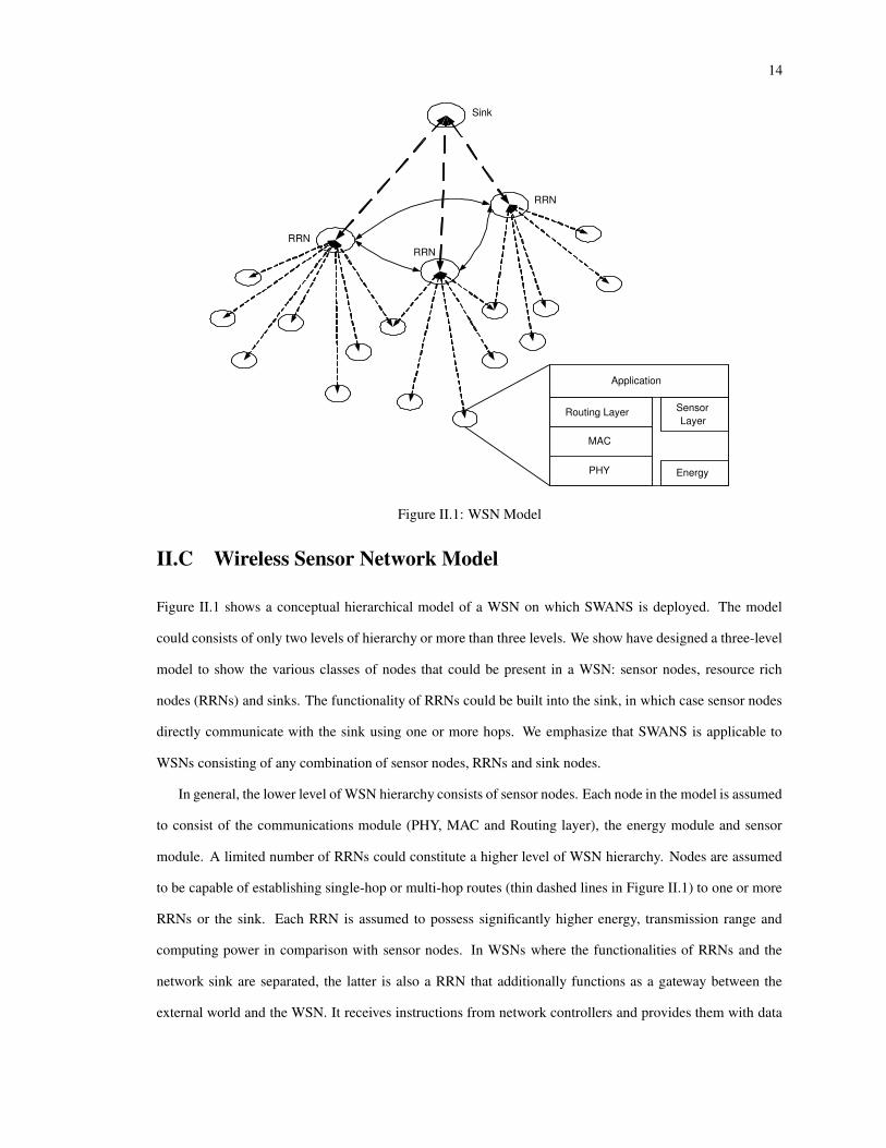
Figure II.1: WSN Model

II.C Wireless Sensor Network Model

Figure II.1 shows a conceptual hierarchical model of a WSN on which SWANS is deployed. The model

could consists of only two levels of hierarchy or more than three levels. We show have designed a three-level

model to show the various classes of nodes that could be present in a WSN: sensor nodes, resource rich

nodes (RRNs) and sinks. The functionality of RRNs could be built into the sink, in which case sensor nodes

directly communicate with the sink using one or more hops. We emphasize that SWANS is applicable to

WSNs consisting of any combination of sensor nodes, RRNs and sink nodes.

In general, the lower level of WSN hierarchy consists of sensor nodes. Each node in the model is assumed

to consist of the communications module (PHY, MAC and Routing layer), the energy module and sensor

module. A limited number of RRNs could constitute a higher level of WSN hierarchy. Nodes are assumed

to be capable of establishing single-hop or multi-hop routes (thin dashed lines in Figure II.1) to one or more

RRNs or the sink. Each RRN is assumed to possess significantly higher energy, transmission range and

computing power in comparison with sensor nodes. In WSNs where the functionalities of RRNs and the

network sink are separated, the latter is also a RRN that additionally functions as a gateway between the

external world and the WSN. It receives instructions from network controllers and provides them with data

15

RRN

Sensor Node

RRN

Routing

MAC

PHY Energy

Sensor

Parameter Values

Monitoring & Reporting

Component Logic Component

Sensor Node

Ontology

Action Component

Sensor Node State

Ontological Symbols

Modify Operational Behavior

State information from all sensor nodes under

this RRN

Monitoring & Reporting

Component

Ontological Symbols Logic Component

Network Ontology

Action Component WSN State

Instruct Sensor Nodes to Modify Operational Behavior

Sensor Node State

I n t e n d e d A c t i o n

Sensor Node State & Intended Action

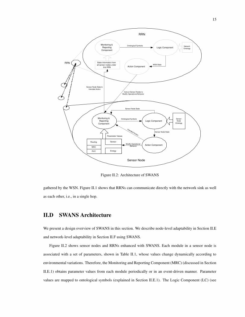
Figure II.2: Architecture of SWANS

gathered by the WSN. Figure II.1 shows that RRNs can communicate directly with the network sink as well

as each other, i.e., in a single hop.

II.D SWANS Architecture

We present a design overview of SWANS in this section. We describe node-level adaptability in Section II.E

and network-level adaptability in Section II.F using SWANS.

Figure II.2 shows sensor nodes and RRNs enhanced with SWANS. Each module in a sensor node is

associated with a set of parameters, shown in Table II.1, whose values change dynamically according to

environmental variations. Therefore, the Monitoring and Reporting Component (MRC) (discussed in Section

II.E.1) obtains parameter values from each module periodically or in an event-driven manner. Parameter

values are mapped to ontological symbols (explained in Section II.E.1). The Logic Component (LC) (see

16

Module ParametersEnergy Remaining Energy Capacity (REC), Energy Consumption Rate (ECR)PHY Received Channel Power (RCP), Received Noise Power (RNP)

Carrier Loss Rate (CLR), Format Violation Rate (FVR)Header Error Check Failure Rate (HFR)

MAC Failed Transmission Ratio (FTR), Multiple Retry Ratio (MRR)Frame Check Sequence Failure Rate (FFR), Collision Ratio (CR)

Routing Number of Reachable RRNs (RR), Number of Paths to RRN (PR)Hop count to RRN (HR), Count of Favored Routers (CFR)Compromised Link Count (CL), Compromised Node Count (CN)Failed Neighbor Count (FN), Node Degree (ND)

Sensor Operating Mode (OpMode), Sensor Accuracy (SA)

Table II.1: Sensor Node Parameters

Section II.E.2) uses ontological symbols as input to a comprehensive sensor node ontology and computes the

sensor node’s state. The Action Component (Section II.E.3) uses rules to determine if and how the sensor

node should modify its operational behavior based on its current state.

In order to ensure that the WSN responds cohesively to environmental variations, SWANS is also de-

ployed on each RRN. As shown in Figure II.2, each RRN obtains current states of sensor nodes in its cluster

either periodically or due to an event. The RRN places each sensor node in a class associated with its state.

For example, all sensor nodes reporting a “Normal” state are placed in a “Sensor Node Normal” class. After

classification, MRC computes the cardinality of each class and maps it to an ontological symbol. LC uses

these symbols as inputs to a network ontology and computes the cluster’s state. The Action Component de-

termines whether the RRN should broadcast a set of instructions to sensor nodes in its cluster to cause them

further modify their operational behavior based on its global view of the network’s state.

The sensor node and network ontologies discussed above can be implemented in two ways: (i) using

a tabular representation and (ii) using a Semantic language such as OWL-DL (Web Ontology Language -

Description Logics) [41].

In the tabular representation, logical values of parameters associated with each module are combined in

boolean expressions to compute the logical state of the module. Subsequently, logical values representing

module states are combined in boolean expressions to compute the logical state of the sensor node. The

tabular representation is useful for WSNs in which a large number of nodes are resource-constrained (e.g.,

Smart Dust motes).

For WSNs containing resource-enhanced sensor nodes (e.g., Wireless Integrated Network Sensor nodes

from Sensoria Corp.) that can support a reasoning engine, SWANS uses richer representations of the sensor

17

node ontology using OWL-DL. Ontologies using OWL-DL explicitly describe logical relationships between

parameters associated with a module, and relationships between module states and sensor node states in a

hierarchical manner. Thus, these ontologies are deployed as an extensible knowledge base on each node.

Logical symbols associated with all monitored parameters at a given instant in time represent an instance

of the sensor node’s “raw” state. Each node provides this instance to the knowledge base, which uses the

reasoning engine to compute and output the logical state of the sensor node.

The network ontology is represented using OWL-DL on RRNs because it contains high-level descriptions

of cluster states and is deployed as a knowledge base on each RRN. Each RRN presents an instance of the

“raw” state of the cluster (consisting of sensor node states and logical values associated with user-defined

constraints) to its knowledge base, which uses a reasoning engine to compute and output the logical state of

the cluster.

II.E Node-Level Adaptability

In this section, we describe the design of the Monitoring and Reporting Component, Logic Component and

Action Component deployed on each sensor node.

II.E.1 Monitoring and Reporting Component (MRC)

The primary tasks of MRC are to obtain values of parameters associated with each module shown in Table

II.1 and map each value to an ontological symbol.

Obtaining Parameter Values

MRC is capable of obtaining parameter values in two ways: periodically and in an event-driven manner.

MRC uses a built-in timer to periodically obtain parameter values. A WSN designer can choose the

periodicity of this process depending upon the needs of the environment in which sensor nodes are deployed.

In the current design of MRC, reporting periodicity is local to each node. Thus, for example, nodes with

greater memory and processor capability can be programmed to monitor and report values of parameters

with greater frequency (i.e., lesser periodicity) than resource-constrained nodes. Further, by ensuring that

each node begins its monitoring process at a different time than its neighbors, the designer can avoid large-

scale collisions in the network due to transmission of status reports by nodes.

18

Value of Parameter Ontological Symbol� ��������� ABNORMAL LOW���������� ������� LOW�������� ������� NORMAL���������� ������� HIGH�������� �� ABNORMAL HIGH

Table II.2: Parameter Mapping

We have also designed MRC to accept parameter values from different modules in an event-driven man-

ner, without waiting for the timer to expire. This mechanism enables a sensor node to be more reactive to its

environment. For example, the PHY module could be instructed to immediately report its current value of

RNP, if three consecutive readings of observed noise power at the wireless interface are above -90 dB in a

previously low-noise environment.

Mapping Parameter Values to Ontological Symbols

SWANS consists of two principal methods of mapping parameter values to ontological symbols.

The general method is to impose thresholds on each parameter based on knowledge about its behavior

within a particular module and associated a symbol with each set of lower/upper thresholds. For example,

consider the parameter representing remaining energy capacity (REC) of a sensor node. Energy consumption

in a sensor node is both hardware dependent (i.e., CPU, RF circuitry, Sensor circuitry) and dependent upon

events occurring in the environment, which may cause the node to become active or inactive. Therefore,

REC cannot be approximated by any specific distribution. In this case, a WSN designer may use additional

information to establish a simple mapping function for REC: for example, if a node currently has more than

40% of its original energy capacity, then REC is NORMAL, otherwise it is ABNORMAL.

A special case of the general method is applicable to parameters whose values either exhibit or can be

approximated by a Gaussian distribution. In this method, parameter values are collected for a fixed period of

time. The mean ( � ) and standard deviation ( � ) of the collected data are computed. Therefore, the collected

data provide information about existing environmental conditions as reflected by � and � for each parameter.

� and � are used to create a set of thresholds to map all subsequent observed values of each parameter to

ontological symbols. Table II.2 shows ranges of parameter values and corresponding ontological symbols.

The method described in this paragraph is not novel. It is commonly used in fuzzy logic to associate linguistic

variables to distributions of states exhibited by an entity in the system.

19

Parameter Value Ontological Symbol0.4TEC REC � TEC NORMAL

0 REC � 0.4TEC ABNORMALECR ���! #"�$%�����& #"#$ ABNORMAL LOW�! #"�$%�����& #"#$� ECR ���# #"#$����' #"�$ LOW�! �"#$%���' �"#$� ECR ���! �"#$��(�& #"�$ NORMAL�! #"�$����' �"#$� ECR ���! �"#$������' #"�$ HIGH� #"�$ ����� �"#$ ECR ABNORMAL HIGH

TEC: Total Energy Capacity, REC: Remaining Energy CapacityECR: Energy Consumption Rate

Table II.3: Energy Module Parameters

We now describe each parameter shown in Table II.1 in detail and show how its values are mapped to

ontological symbols using one of the two methods described above.

Energy Module

The energy module describes a sensor node’s state as a function of its energy consumption. Table II.3 shows

the mapping for parameters REC and ECR. The acronym TEC stands for Total Energy Capacity. A threshold

of 40% is chosen to indicate normal or abnormal levels of remaining energy capacity. A sensor node’s

ECR allows it to determine how quickly its energy is being drained. A very low rate (ABNORMAL LOW)

could indicate node malfunction, whereas a very high rate (ABNORMAL HIGH) could indicate a resource

starvation attack in progress. The state space associated with the Energy module theoretically consists of a

maximum of ten different states; however, when ECR takes on extreme values such as ABNORMAL LOW

or ABNORMAL HIGH we disregard the value of REC and declare that the energy module is in an abnormal

state, causing an overall reduction in the state space associated with the energy module. We discuss possible

states of the energy module in Section II.E.2.

PHY Module

Table II.4 maps values of parameters RCP, RNP, CLR, FVR and HFR – which are associated with the PHY

module - to ontological symbols. RCP is NORMAL if it is above -80 dBm, which is equivalent to )+*-,/.mW. Similarly, RNP is NORMAL if it is below -80 dBm. CLR, FVR and HFR are assumed to be Gaussian

variables. CLR tracks the rate of carrier loss, which is signaled at the wireless interface if the channel becomes

idle after the interface has received a synchronization symbol and validated the header of the incoming data

frame. FVR indicates the rate at which frames violating the prescribed format are received at the interface.

20

Parameter Value Ontological Symbol-80 dBm RCP NORMAL

RCP � -80 dBm ABNORMALRNP -90 dBm NORMAL-80 dBm RNP ABNORMAL

CLR ��� "�01$ ��� "�01$ NORMALCLR 23� "#01$ �(� "#01$ HIGHCLR 2�� "#01$ ����� "�01$ ABNORMAL HIGHFVR ���!465!$��(�&4�5�$ NORMALFVR 2��!4�5�$����'465#$ HIGHFVR 23�!4�5#$������&4�5�$ ABNORMAL HIGHHFR ���!7 4#$ ���'7 4!$ NORMALHFR 2�� 7 4!$%�(� 7 4#$ HIGH

HFR 23� 7 4!$������ 7 4!$ ABNORMAL HIGHRCP: Received Channel Power, RNP: Received Noise PowerCLR: Carrier Loss Rate, FVR: Format Violation RateHFR: Header Error Check Failure Rate

Table II.4: PHY Module Parameters

HFR tracks the rate at which frames failing the header error check are received at the interface. Low values of

these variables generally indicate normal conditions, whereas higher rates of loss or failure are indicative of

sleep deprivation or denial-of-service attacks. CLR is a transmit-side parameter, i.e., it describes the state of

PHY when this node is a transmitter because carrier loss is indicated on the node that initiated transmission.

Similarly, FVR and HFR are receive-side parameters, i.e., they describe PHY state when this node is a

receiver, because format violation and HEC failure are detected on the receiver.

The state space associated with the PHY module is theoretically associated with a hundred and eight

states; however, based on the above discussion, we observe that a large number of states become redundant

under certain conditions. For example, if either RCP or RNP is in the ABNORMAL state, then the values of

the remaining parameters can be disregarded, thus reducing the state space considerably. Similarly, if one of

FVR and HFR is in the ABNORMAL HIGH state, then the state of the PHY state can be identified clearly

even after disregarding values of other parameters. We discuss possible states of the PHY module in Section

II.E.2.

MAC

As shown in Table II.5, the MAC module is associated with four parameters: FTR, which tracks the number

of MAC frames for which no acknowledgment is received; MRR, which tracks the number of frames that

had to be retransmitted before successful reception (i.e., acknowledgment received); FFR indicates the rate at

21

Parameter Value Ontological SymbolFTR ��� 4!8-$ ��� 4#8&$ NORMALFTR 2�� 4#8&$ ��� 4!8-$ HIGH

FTR 2�� 4#8&$ ����� 4!8-$ ABNORMAL HIGHMRR ���#9:$;$%�(�-9<$;$ NORMALMRR 2���9<$;$%���&9:$;$ HIGH

MRR 2��#9:$;$%�����&9:$;$ ABNORMAL HIGHCR ��� "#$ �(� "#$ NORMALCR 2��!"�$����'"�$ HIGH

CR 23�!"�$������&"#$ ABNORMAL HIGHFFR ���!4!4!$����'4!4!$ NORMALFFR 2��!4#4!$����'4#4!$ HIGHFFR 2�� 4!4#$ ����� 4!4!$ ABNORMAL HIGH

FTR: Failed Transmission Ratio, MRR: Multiple Retry RatioCR: Collision Ratio, FFR: Frame Check Sequence Failure Ratio

Table II.5: MAC Module Parameters

which frames with an invalid Frame Check Sequence (FCS) are received; and CR, which tracks the number

of frames discarded due to collisions. Again, lower values (i.e., at most one standard deviation greater than

the mean) indicate that the MAC module’s state is normal. Higher values indicate the possibility of sleep

deprivation and denial-of-service attacks. FTR and MRR are transmit-side parameters. CR and FFR are

receive-side parameters. Thus, we observe that the seven parameters associated with PHY and MAC can

provide important information regarding how transmission and reception are being affected on a node.

The state space of the MAC module is theoretically associated with eighty-one states. This space is

reduced by declaring that the transmit side is in an alert/abnormal state when one of FTR and MRR is

HIGH/ABNORMAL HIGH or that the receive side is in an alert/abnormal state when one of CR and FFR

has an HIGH/ABNORMAL HIGH value, respectively. We discuss possible states of the MAC module in

Section II.E.2.

Routing

The routing module is associated with eight parameters: the number of Reachable RRNs (RR), the number

of Paths to a chosen or designated RRN (PR), the hop-count to a chosen or designated RRN (HR), a count

of favored routers (CFR), the node degree (ND), the number of compromised nodes (CN), the number of

compromised links (CL) and the number of failed neighbors (FN). For readability, we show these parameters

and associated symbols in two tables.

Table II.6 shows the mapping for RR, PR, HR and CFR. Table II.7 shows the mapping for CN, CL, FN

22

Parameter Value Ontological SymbolTRR*(1 - r1) � RR � TRR*(1 + r1) NORMAL

TRR*(1 - r2) � RR TRR*(1 - r1) LOWRR TRR*(1 - r2) ABNORMAL LOW

TRR*(1 + r1) RR � TRR*(1 + r2) HIGHRR 2 TRR*(1 + r) ABNORMAL HIGH

TPR*(1 - p1) � PR � TPR*(1 + p1) NORMALTPR*(1 - p2) � PR TPR*(1 - p1) LOW

PR TPR*(1 - p2) ABNORMAL LOWTPR*(1 + p1) PR � TPR*(1 + p2) HIGH

PR 2 TPR*(1 + p2) ABNORMAL HIGHTHR*(1 - h1) � HR � THR*(1 + h1) NORMAL

THR*(1 - h2) � HR THR*(1 - h1) LOWHR THR*(1 - h2) ABNORMAL LOW

THR*(1 + h1) HR � THR*(1 + h2) HIGHHR 2 THR*(1 + h2) ABNORMAL HIGH

TR*(1 - m1) � CFR � TR*(1 + m1) NORMALTR*(1 - m2) � CFR TR*(1 - m1) LOW

CFR TR*(1 - m2) ABNORMAL LOWTR*(1 + m1) CFR � TR*(1 + m2) HIGH

CFR 2 TR*(1 + m2) ABNORMAL HIGHTRR: Total Reachable RRNs, RR: Reachable RRN countTPR: Total Paths to each RRN, PR: Path count to RRNsTHR: Total Hop count to each RRN, HR: Hop-count to RRNsTR: Total Router count, CFR: Count of Favored Routers

Table II.6: Routing Module Parameters I

and ND. Each pair of ( =>)@?A=�� ), (#)@?B/� ), ( C#)�?DC&� ), ( EF)�?GE�� ) and ( H!I')@?AH!IJ� ) is tunable and represents a fraction

between 0 and 1, of the established value of the corresponding parameter. Parameters TRR, TPR, THR, TR

and TND are set during network self-organization. (The letter T in TRR, TPR, THR, TR and TND stands

for Total.) For example, each node knows the number of RRNs it can reach based on first hand knowledge

(i.e., it discovered them) or that provided by neighbors (i.e., node X has a one-hop neighbor Y that can reach

2 RRNs, therefore X can too). Thus, by tracking changes to these parameters, a node can determine the

state of its routing module. Variable pairs ( =J)�?G=K� ), (#)@?B-� ), ( C#)�?DC&� ), ( EF)�?AE�� ) and ( H!I&)�?GH!I>� ) provide this

functionality.

Parameters CN, CL and FN are dependent upon ND. Variable c represents a fraction of the total number of

neighbors that may be compromised before CN is declared ABNORMAL. Variable f has a similar function

for FN, the failed neighbor count. CL is the number of links established by this node which have been

compromised. CL tracks CN, the number of compromised neighbors. Thus, CL must be less than or equal to

CN; otherwise it is considered ABNORMAL.

23

Parameter Value Ontological SymbolTND*(1 - nd1) � ND � TND*(1 + nd1) NORMAL

TND*(1 - nd2) ND TND*(1 - nd1) LOWND TND*(1 - nd2) ABNORMAL LOW

TND*(1 + nd1) ND � TND*(1 + nd2) HIGHND 2 TND*(1 + nd2) ABNORMAL HIGH

CN � TND*c NORMALCN 2 TND*c ABNORMALCL � CN NORMALCL 2 CN ABNORMAL

FN � ND*f NORMALFN 2 ND*f ABNORMAL

TND: Total Node Degree, ND: Node DegreeCN: Compromised Nodes, CL: Compromised LinksFN: Failed Neighbors

Table II.7: Routing Module Parameters II

Parameter Value Ontological SymbolOpMode == ACTIVE L OFF NORMAL

OpMode == HIGH SAMPLING L LOW SAMPLING ABNORMAL0.3 SA � 1.0 NORMAL0.0 SA � 0.3 ABNORMAL

OpMode: Operating Module, SA: Sensor Accuracy

Table II.8: Sensor Module Parameters

The state space associated with the routing module theoretically consists of twenty-five thousand states.

We observe, however, that when either a combination of RR, PR and CFR (shown in Table II.6) or only one of

them has an ABNORMAL HIGH value, then the state of the routing module can be identified by disregarding

other parameters. This is because, at the level of individual nodes, detecting an abnormally high number of

RRNs, paths or routers should be considered an attack irrespective of other parameter values. Further, when

either of RR, PR, CFR and ND has an ABNORMAL LOW value, then the node can be declared to be either

in a “disconnection imminent” or a “disconnected” state, irrespective of other parameter values. This is

because, the inability of a node to reach a prescribed number of RRNs due to loss of RRNs, path failure or

router failure is an indication that it is about to be disconnected from the WSN, if not already disconnected.

We have reduced the state space of the routing module using similar reasoning. It is discussed in Section

II.E.2.

24

REC ECR Energy StateN N Normal EnergyN L Malfunction ImminentN AL Malfunction IndicatedN H Low Energy ImminentN AH Discharge ImminentA N Low EnergyA H M AH Discharged

REC: Remaining Energy CapacityECR: Energy Consumption RateN: Normal, A: Abnormal, H: HighAL: Abnormal Low, AH: Abnormal High

Table II.9: Energy Module State

Sensor Module

Parameters associated with the Sensor module are operating mode (OpMode) and accuracy (SA). Together,

OpMode and SA provide information to determine the usefulness of a particular sensor under existing envi-

ronmental conditions. The energy consumption of a sensor per epoch can be computed based on its operating

mode. For example, a sensor operating in a HIGH SAMPLING mode consumes more energy than in the

ACTIVE operating mode. The accuracy of a sensor depends upon many factors, internal and external. While

internal factors are mostly static (e.g., drift), external factors in the form of physical environmental variables

(e.g., temperature, pressure, humidity, wind velocity) may be highly varying. Such variations can severely

affect the accuracy and in some cases, cause the sensor data to become useless. We have designed a sensor

data calibration algorithm [3] that allows a sensor node to automatically calibrate or correct data output by

a sensor layer. Thus, the node can compute the accuracy of each sensor layer based on the observed output

and the correct output. Table II.8 shows symbols associated with operating mode and sensor accuracy.

II.E.2 Logic Component (LC)

LC is responsible for computing the state of each module on a sensor node based on values of parameters as-

sociated with each module. It also computes sensor node state by logically combining module states obtained

in the previous step.

25

HFR FVR CLR RNP RCP PHY StateN N N N N NormalN N N X A Out-of-RangeN N N M H H M N N Jamming ImminentN N N M AH AH M N N Jammed

N M H H M N N N N Abnormal Rx ImminentN M AH AH M N N N N Abnormal RxH M X H M X H M X H M X N Denial-of-Service Imminent

AH M X AH M X AH M X AH M X N Denial-of-ServiceRCP: Received Channel Power, RNP: Received Noise PowerCLR: Carrier Loss Rate, FVR: Format Violation RateHFR: Header Error Check Failure RateN: Normal, A: Abnormal, H: High, AH: Abnormal High, X: Don’t Care

Table II.10: PHY Module State

Energy Module

Table II.9 shows possible ECR and REC values along with their combinations that reflect a node’s energy

state. A low or abnormally low rate of energy consumption during its active cycle is an indicator of a node’s

malfunctioning state. This is because, in active mode, various components of the node must consume a fixed

amount of energy, per hardware characteristics. When the energy module exhibits a high rate of consumption,

the sensor node could reach a low energy state, indicating the possibility of an attack against the node. An

abnormally high rate of energy consumption is an indication of a sleep deprivation torture attack [56] and

points to the likelihood that the node will be completely discharged of its energy. A low energy condition

is indicated when the node’s rate of energy consumption is normal, but its remaining energy capacity is

abnormal. When both REC and ECR are abnormal, it is highly likely that the sensor node will completely

exhaust its energy.

PHY Module

Boolean expressions for PHY parameters and their combinations are shown in Table II.10. If RCP is abnor-

mal, then PHY is Out-of-Range, which implies that the node is out of communication range of its neighbors.

A potential indication of jamming is exhibited by the PHY module if either or both of RNP and CLR have

high values. When they have abnormally high values, then the PHY module is considered to be jammed.

This situation occurs when background noise level rises above transmission or reception power. It could also

occur when a significant number of transmissions experience carrier signal loss. PHY exhibits resource star-

vation, indicated by high or abnormally high values of FVR and HFR when a significant number of received

26

FTR MRR FFR CR MAC StateN N N N NormalN N N M H H M N Abnormal Reception ImminentN N N M AH AH M N Reception Abnormal

N M H H M N N N Abnormal Transmission ImminentN M AH AH M N N N Transmission AbnormalN M H H M N X X Abnormal Tx+Rx Imminent

N M AH AH M N X X Abnormal Tx+RxFTR: Failed Transmission Ratio, MRR: Multiple Retry RatioCR: Collision Ratio, FFR: Frame Check Sequence Failure RatioN: Normal, H: High, AH: Abnormal High, X: Don’t Care

Table II.11: MAC Module State

frames are malformed, i.e., have an illegal format or fail the header error check. This situation could occur if

an adversary possessing sufficient resources were to continuously broadcast malformed frames to legitimate

sensor nodes. When one or more of HFR, FVR, CLR and RNP have high or abnormally high values, with

RCP remaining normal, a Denial-of-Service attack against the node is indicated.

MAC Module

Table II.11 shows possible states of the MAC module. The receive-side of the MAC module exhibits a po-

tentially abnormal state when either CR or FFR or both have high values. When these values are abnormally

high, the MAC module’s abnormal state at its receiver is confirmed. The discussion presented for receive-

side behavior at the PHY module (i.e., for FVR and HFR) applies in this case too. The MAC module is in

an abnormal state at its transmit-side if FTR or MRR or both have high or abnormally high values. This

situation occurs when MAC frames transmitted by a node are not ACKnowledged, thereby causing failed

transmissions or multiple retransmissions before succeeding. Nodes in exhibiting this behavior are likely to

exhaust their energy resources even faster than those exhibiting receive-side abnormalities due to high energy

costs associated with transmission. When a combination of all four parameters have high or abnormally high

values, the MAC module is in an abnormal state on both transmissions and receptions, indicating a possible

denial-of-service attack against the node.

Routing Module

Table II.12 shows states of the routing module as indicated by the number of reachable RRNs (RR), number

of paths to RRNs (PR), number of hops to RRNs (HR), number of routers (CFR), number of compromised

27

RR PR HR CFR CL CN FN ND Routing StateN N N N N N N N Normal

L M X L M X H M X L M X N N A L Disc. Imm.AL M X AL M X AH M X AL M X N N A AL DisconnectedH M AH H M AH N H M AH N N N N Ab. Rt. Info.

N N N N N N N H M AH High Node DegreeN M H M AH N M H M AH L M AL N N N N N M AH Ab. Dist. Info.

N N N N X A N X CompromisedL M AL L M AL H M AH L M AL X A A L M AL DoS

RR: Reachable RRN count, PR: Path count to RRNsHR: Hop-count to RRNs, CFR: Count of Favored RoutersND: Node Degree, CN: Compromised Nodes, CL: Compromised Links, FN: Failed NeighborsAb. Rt. Info.: Abnormal Routing InformationAb. Dist. Info.: Abnormal Distance InformationN: Normal, L: Low, AL: Abnormal Low, H: High, AH: Abnormal High, X: Don’t Care

Table II.12: Routing Module State

links (CL), number of compromised neighbors (CN), number of failed neighbors (FN) and the node degree

(ND).

Node disconnection is imminent when RRN reachability is low, an abnormal number of neighbors have

failed and overall node degree is low. Disconnection is confirmed when RRNs are unreachable and overall

node degree is abnormally low. When all routing indicators, except ND (high or abnormally high), are

normal the routing module indicates that a significant number of new nodes have been discovered in its

neighborhood. These nodes may be due to legitimate node addition or due to a node addition attack [61].

The routing module indicates that it has obtained abnormal routing information (i.e., count of RRNs, paths

and routers) when RRN reachability indicators (RR, PR, CFR) have high or abnormally high values. This

situation occurs when a node’s neighbors begin to disseminate bogus routing information. One of the methods

of spreading such information in a sensor network is to claim to provide to routes to either existing or non-

existent cluster-heads. The routing module indicates that it has received abnormal distance information when

RRN reachability indicators have normal or high values, but HR has a low or abnormally low value. This

situation could occur when the node is under a distance-based attack. A distance-based attack, such as

Wormhole or Sinkhole, is one in which adversaries advertise minimum hop distances to RRNs and sinks,

which are eventual destinations of data from all ordinary sensor nodes. Thus, adversaries attract traffic toward

themselves and subsequently launch different types attacks [31]. Neighborhood compromise is indicated

when the number of compromised neighbors of a sensor node exceeds the prescribed threshold. In general,

depending upon the security protocol, the number of compromised links associated with a node (CL) tracks

28

OpMode SA Sensor StateN N NormalN A Low AccuracyA N High Energy ConsumptionA A Non-functional

OpMode: Sensor Operating Mode, SA: Sensor AccuracyN: Normal, A: Abnormal

Table II.13: Sensor Module State

CN, so that both are equal. However, in certain cases extra information may become available to the adversary

upon node compromise thereby enabling the compromise of more links. In that case CL 2 CN. When

RRN reachability indicators and neighbor compromise indicators have abnormal values, the routing module

indicates a DoS attack.

Sensor Module

Table II.13 shows that values of parameters OpMode and SA directly reflect the sensor module’s state. When

both parameters have abnormal values, the sensor is non-functional if neither its accuracy can be improved

nor energy consumption reduced.

Sensor Node States

The Logic Component computes the logical state of a sensor node after computing logical states of Routing,

MAC, PHY, Energy and Sensor modules, described in previous sections. We show examples of boolean ex-

pressions that assign logical states to a sensor node. Symbols RS, MS, PS, ES, SS and NS stand for Routing

State, MAC State, PHY State, Energy State, Sensor State and Node State, respectively. The notation XS(Y)

in each expression below indicates the logical value Y assigned to module X. Further, values of terms absent

in any expression are assumed to be “Normal”.

RS(Normal) N MS(Normal) N PS(Normal) N ES(Normal) N SS(Normal) O NS(Normal)

ES(Discharged) O NS(Non-functional)

(MS(Abnormal Tx) M PS(Jammed)) N ES(Low Energy) O NS(Jammed)

29

((MS(Abnormal Rx) M PS(Abnormal Rx)) N ES(Low Energy Imminent)) O NS(Resource Starvation)

(RS(Disconnected) M PS(Out-of-Range)) O NS(Disconnected)

RS(Abnormal Routing Info.) O NS(Node Addition Attack)

ES(Low Energy Imminent) N SS(High Energy Consumption) O NS(Low Sensitivity)

As shown in Figure II.2, LC returns the sensor node’s logical state to MRC, which in turn, transmits this

information to a RRN.

II.E.3 Action Component (AC)

Sensor nodes modify their operational behavior according to states determined by LC. An important param-

eter that a sensor node employs in deciding its operational behavior is its previous state as determined by LC.

If both previous and current states are equal, then the node’s operational behavior would not change. If none

of the sensor nodes modify their operational behavior, then the WSN’s behavior would also remain the same.

AC contains a set of rules that are applied based on the sensor node’s logical state, computed by LC.

In this section, we show examples of actions that a node can take in response to environmental variations,

reflected in its logical state. The list of actions shown in this section is by no means exhaustive; a WSN

designer may add rules to AC describing additional actions for each sensor node. (OS in the expressions

below stands for Operational State.)

NS(Jammed) M NS(Resource Starvation) M (NS(Disconnected) N ES(Low Energy)) O OS(Sleep)

The above rule causes nodes under jamming or resource starvation attacks to transition from an active oper-

ational state to a Sleep state. Nodes with low energy that have been disconnected from the network due to

neighbor failure or route failure and that are at low energy levels also enter the sleep state. The primary goal

of nodes taking this action is to conserve energy and await a change in environmental conditions (e.g., death

of malicious nodes causing jamming or resource starvation, addition of new nodes to re-establish broken

30

links). As we discuss in Section II.F.3 below, RRNs may override a node’s decision to sleep. Many energy

management solutions in WSNs focus on sleep-scheduling, i.e., establishing a sequence of sleep and wake

times for each node in the WSN, such that nodes spend a large part of their life in sleep mode as opposed to

active mode. The above rule fits this type of node behavior because if a node detects either an attack or that it

cannot reach the rest of the network, it can simply transition back to sleep mode after informing a RRN about

its state.

NS(Disconnection Imminent) N ES(Normal) O OS(Increase Tx Range)

If sensor nodes possess on-board radios capable of varying their transmission range, then the WSN can adapt

to the situation in which a node or set of nodes would be disconnected from the network due to neighbor fail-

ure or death. Thus, according to the above rule, if a node detects an imminent disconnection from the WSN

and its energy level is normal, then it attempts to reconnect to the network by increasing its transmission

range. In this manner, a node may reach either a RRN directly or nodes closer to a RRN, thereby reducing its

hop count. However, this action should be temporary, because long-range transmission costs could quickly

deplete the node’s energy.

NS(High Node Degree) M NS(Low Accuracy) M NS(Abnormal Routing Info.) O OS(Extend Active Pe-

riod)

According to the above rule, a node that can control its sleep schedule can extend the period during which it

remains active in response to topological variations (i.e., increase in node degree, receipt of abnormal routing

information) or loss of sensitivity of on-board sensors (e.g., fog affects on-board camera). By remaining

active during node addition, which may be legitimate or malicious, a node can ensure that only legitimate

nodes are able to join the network using built-in security mechanisms or raise an alarm that malicious nodes

have attacked the network. Similarly, if a node receives abnormal routing information, then it remains active

to determine whether the information was sent in error or is being transmitted by a malicious adversary. Loss

of sensor accuracy on a sensor node could imply an overall reduction in the accuracy of the WSN. Thus, a

node remains active for a longer period of time to either gather more data and make up for loss in accuracy or

to detect a change in conditions affecting accuracy (e.g., camera remains active to show fog lifting and new

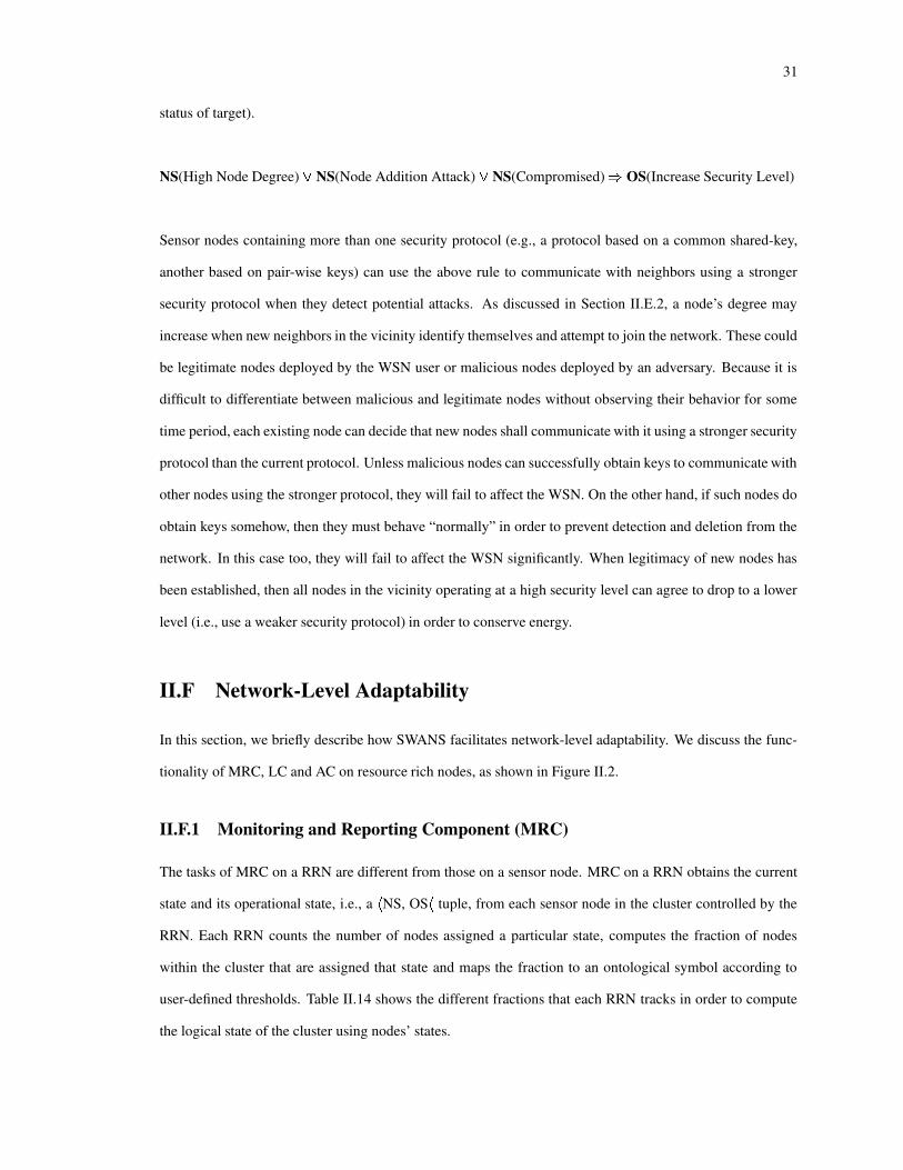
31

status of target).

NS(High Node Degree) M NS(Node Addition Attack) M NS(Compromised) O OS(Increase Security Level)

Sensor nodes containing more than one security protocol (e.g., a protocol based on a common shared-key,

another based on pair-wise keys) can use the above rule to communicate with neighbors using a stronger

security protocol when they detect potential attacks. As discussed in Section II.E.2, a node’s degree may

increase when new neighbors in the vicinity identify themselves and attempt to join the network. These could

be legitimate nodes deployed by the WSN user or malicious nodes deployed by an adversary. Because it is

difficult to differentiate between malicious and legitimate nodes without observing their behavior for some

time period, each existing node can decide that new nodes shall communicate with it using a stronger security

protocol than the current protocol. Unless malicious nodes can successfully obtain keys to communicate with

other nodes using the stronger protocol, they will fail to affect the WSN. On the other hand, if such nodes do

obtain keys somehow, then they must behave “normally” in order to prevent detection and deletion from the

network. In this case too, they will fail to affect the WSN significantly. When legitimacy of new nodes has

been established, then all nodes in the vicinity operating at a high security level can agree to drop to a lower

level (i.e., use a weaker security protocol) in order to conserve energy.

II.F Network-Level Adaptability

In this section, we briefly describe how SWANS facilitates network-level adaptability. We discuss the func-

tionality of MRC, LC and AC on resource rich nodes, as shown in Figure II.2.

II.F.1 Monitoring and Reporting Component (MRC)

The tasks of MRC on a RRN are different from those on a sensor node. MRC on a RRN obtains the current

state and its operational state, i.e., a P NS, OS P tuple, from each sensor node in the cluster controlled by the

RRN. Each RRN counts the number of nodes assigned a particular state, computes the fraction of nodes

within the cluster that are assigned that state and maps the fraction to an ontological symbol according to

user-defined thresholds. Table II.14 shows the different fractions that each RRN tracks in order to compute

the logical state of the cluster using nodes’ states.

32

Module ParametersEnergy Non-Functional Node Fraction (NFN), Low-Energy Node Fraction (LEN)

Communications Jammed Node Fraction (JN), Starved Node Fraction (SN)(PHY, MAC, Routing) Fraction of Nodes under DoS (NDOS)

Fraction of Nodes under Distance Attack (NDA)Fraction of Nodes under Node-based Attack (NNA)Fraction of Compromised Nodes (NC)Fraction of New Nodes (NN)Fraction of Nodes Requesting Neighbor Deletion (NRD)

Sensor Fraction of Nodes with High Energy Consuming Sensors (NHES)Fraction of Nodes with Low Accuracy Sensors (NLAS)

Table II.14: RRN Parameters

Thus, for example, if the fraction of jammed nodes (JN) is greater than 5% of the total size of the cluster,

then the RRN maps the value of JN to ABNORMAL. Similarly, a 20% increase in the fraction of new nodes

(NN) in the cluster results in mapping it to an ABNORMAL value. The RRN provides ontological symbols

of the twelve parameters shown in Table II.14 to the Logic Component as input and obtains the cluster’s

current state.

II.F.2 Logic Component

The LC on a RRN functions in a manner similar to that on a sensor node. It employs a cluster ontology to

compute logical states of the Energy, Communications and Sensor modules in the cluster, which it subse-

quently combines to obtain the logical state of the cluster as a whole.

For example, communications in the cluster are under short-term attack if either an abnormal number of

nodes is under a jamming attack or a resource starvation attack. On the other hand, cluster communications

are under long-term attack if different parts of the cluster experience a node-based attack, a distance-based

attack and a DoS. Further, if the fraction of low energy nodes in the cluster is high, but overall sensor behavior

is normal, then cluster communications under long-term attack combined with low energy in cluster results

in the cluster’s overall state: cluster failure imminent.

Other states of the cluster are computed using similar logical combinations.

II.F.3 Action Component

On a RRN, the Action Component combines the output of the Logic Component with user-defined constraints

(if any) and aggregate sensor data to determine the cluster’s response to the observed environmental variation.

33

In this section, we show examples of rules used by RRNs for this purpose. In each case, CS stands for Cluster

State.

CS(Under SDTA) N Detected(A) N Detects(S, A) N NS(S, Sleep) O NS(S, Active)

The above rule states that under a Sleep Deprivation Torture Attack (SDTA), all sensor nodes S in the cluster

that can detect malicious agent type A, and have transitioned to the Sleep state must transition back to the

Active state, if the agent has been detected. The rationale behind this rule is as follows: The adversary, being

aware of the WSN’s presence around a resource or asset, first attacks the network via SDTA in order to force

nodes to go to Sleep (and conserve energy) and subsequently attacks the resource using some agent (e.g.,

biological agent such as Anthrax). Therefore, when it detects SDTA and the presence of a malicious agent,

the network must ensure that all sensor nodes capable of tracking the agents remain active, even at the risk of

exhausting them completely.

CS(Normal) N Detected(A) N Detects(S, A) O Stop Aggregation(S)

According to the above rule, the network instructs sensor nodes capable of detecting a certain agent A to

stop aggregating data and instead transmit raw data values, when traces of the agent have been detected.

Such a situation could occur, for example, in the case of a WSN deployed to detect a biological, chemical

or radiation event. By obtaining raw data values from individual sensor nodes, the RRN can obtain precise

information about the concentrations of the agent in each region, instead of receiving a single, less accurate,

aggregate data value. The pre-condition that the Cluster State be Normal ensures that this rule is executed

only when the network has sufficient energy to handle large data streams that will result from transmission of

individual data values across the network.

Rules similar to the ones described in this section can be implemented either in a logic programming

language, such as Prolog, or as a policy using a policy language.

34

Parameter ValueField size 600 x 500

Node transmission range 75.0 mNetwork size 100 to 800 nodes

Initial node energy 1000 JRC5 encrypt/decrypt energy consumption 0.76 � J/byte

Table II.15: WSN Configuration Parameters

II.G Experimental Evaluation of SWANS

We describe three experiments to evaluate SWANS and demonstrate its ability to ensure that WSNs can

detect, classify and respond to environmental variations. The three variations we consider are: (i) increase in

network size (topological/security variation), (ii) sleep deprivation torture attack (security variation) and (iii)

significant node failure (topological variation). Sections II.H, II.I and II.J describe experiments evaluating

SWANS according to each of these three variations, respectively.

We have simulated SWANS using J-Sim [55], a Java-based simulator developed jointly by students and

faculty at The Ohio State University and University of Illinois at Urbana-Champaign. The simulator uses an

autonomous component programming model, in which each entity is a component as opposed to an object.

Components communicate via input and output ports, passing parameters via contracts. J-Sim contains a

wireless sensor network simulation package, which we modified and augmented to implement SWANS.

We assume that wireless sensor nodes are deployed in the area of interest along with RRNs and sinks.

Each node is capable of discovering its neighbors and establishing secure links with them. A node has the

capability to create secure links using symmetric keys, which may be common shared keys (low security)

or unique, pair-wise keys (high security). As an initial condition, we assume that each node uses common,

shared keys to establish secure links.

Table II.15 shows a set of parameters, common to all three experiments, used in the evaluation. We

observe that the maximum network size in each experiment is 800 nodes because the Java Virtual Machine

was unable to provide memory to the J-Sim simulator to support larger network sizes.

II.H Adaptability to Increase in Network Size

In this section, we describe an experiment to demonstrate the ability of an established WSN to adapt to

increases in network size due to the addition of new nodes, legitimate or malicious. We show how a WSN

35

dynamically increases its security level depending upon the number of new nodes attempting to join the WSN.

We contrast an adaptive WSN to non-adaptive WSNs that cannot modify their security level and maintain

either a low security level (thereby consuming less energy) or a high security level (thereby consuming more

energy).

Node addition may be a legitimate process carried out periodically to ensure the WSN’s survival or a

process initiated by some adversary intent on disrupting network functionality, i.e., a node addition attack.

SWANS enables nodes in a WSN to adapt to both types of node addition. In the following sections, we

discuss the role that each SWANS component plays in WSN adaptivity to node addition. We also evaluate

WSN performance in terms of energy consumption and discuss trade-offs in terms of security and energy.

II.H.1 The Node Addition Process

Node addition is a common, legitimate process associated with WSNs. Based on the type of WSN and the

area of deployment, node addition may either be periodic or event-driven. For example, WSNs deployed

in a building are more likely to require periodic replenishment of nodes as opposed to WSN deployed on a

battlefield, which may require new nodes based on certain events. Further, adversaries in hostile environments

may seek to add malicious nodes to the network to disrupt it and/or passively gather data for future misuse.

In general, legitimate node addition is accomplished as follows. Upon deployment, new nodes attempt

discover existing nodes within their transmission range. The latter respond to the discovery request and

subsequently, both parties establish a secure link using the default security protocol.

Using SWANS, each node determines the most appropriate mechanism of accepting new neighbors based

on values of its current and original node degree. These mechanisms allow a node to accept new neighbors

using the default security protocol or at higher levels of security. The transition from a lower to a higher

security level is triggered when the node degree crosses bounds established by the WSN designer.

A WSN designer uses SWANS to set appropriate lower and upper bounds on the node degree based on

the area of deployment and the potential for attacks against the network. For example, let ( H!I') , H!I>� ) shown

in Table II.6 have the following values: H!I&):�Q*'R S and H!IJ���T)�R * . Assume that the current value of node

degree is 10. Thus, as long as it is between 5 and 15, node degree is considered Normal. When it crosses 15,

node degree is considered High and triggers a raise to the next higher security level. When its degree crosses

20, i.e., more than doubles, a node is considered under attack, thereby triggering a transition to the highest

security level before allowing new neighbors to join its neighborhood. Therefore, by choosing the values of

36

Parameter ValueNode degree threshold, nd1 0.5Node degree threshold, nd2 1.0

Energy consumed per node at SL0 2.432e-5 J/msgEnergy consumed per source/dest. node at SL1/SL2 4.256e-5 J/msg

Min. energy consumed per intermediate node at SL1/SL2 3.648e-5 J/msgMax. energy consumed per intermediate node at SL1/SL2 7.296e-5 J/msg

Table II.16: Experiment Parameters

Data Field

Destination Source DstRouter Nonce Data SrcRouter Label

Address Fields

4 bytes 4 bytes 4 bytes 4 bytes 4 bytes 4 byte 8 bytes

Figure II.3: Message Format

nd1 and nd2 carefully, a WSN designer can ensure that all nodes in the network operate at the appropriate

security level and can communicate with a sufficient number of neighbors.

The trade-off in this case is directly between the WSN’s security and its energy consumption. Smaller

values for nd1 and nd2 will cause nodes to transition to higher security levels quicker and consume more

energy, whereas larger values for nd1 and nd2 allow nodes to consume less energy by operating at lower

security levels. The values chosen for nd1 and nd2 also determine the frequency with which nodes transition

to the highest security level due to changes in node degree. The smaller the values of nd1 and nd2, the greater

the probability of transition to the highest security level.

II.H.2 Results

Table II.16 shows various parameters and their values used in the simulation. We assume that each node

can monitor its degree with respect to prescribed lower and upper bounds. Each node uses the ontology in

SWANS to determine its logical state. The action component on each node causes it to transition to one of

three operational states: Maintain Security Level, Raise Security Level and Drop Security Level.

In the simulation, WSN sizes range from 100 to 800 nodes. The number of RRNs is fixed at 1% of the

network size. For the purpose of discussing security versus energy trade-offs, we present the case of a 200-

node WSN, including 2 RRNs. The network also consists of a single sink node. All nodes in the WSN are

immobile, except for a target node that moves randomly through the network, periodically emitting a signal.

When sensor nodes within range of the target receive this signal they transmit a signal-to-noise (SNR) value

37

to their respective RRNs via established routes. Thus, the SNR value from each node finally reaches the

sink. The message format that nodes use to transmit data values is shown in Figure II.3. Energy consumption

values per message at SL0, SL1 and SL2 (explained below) shown in Table II.16 are based on this message

format.

We assume that each node can use three different security levels for secure communication and topology

management (i.e., node addition and deletion, route computation etc.). Security levels are synonymous with

the keying mechanism employed by nodes in the WSN. Thus, at the lowest level of security, SL0, all nodes use

a common, shared key for secure communication. At SL1, a group of nodes initiate and exchange pair-wise

symmetric keys using a distributed protocol (D-SONETS in this experiment). At SL2, each node transmits

a list of neighbors to its RRN requesting keying material using which it computes pair-wise keys with those

neighbors (C-SONETS in this experiment). Thus, SL2 provides an authentication mechanism in which nodes

joining the network receive key material after a RRN verifies their identities.

In this simulation, each node tracks energy consumed for secure communication when operating at differ-

ent security levels. Thus, we can analyze the trade-off between operating at a particular level versus energy

consumption, based on changing node degree. Initially, each node is assumed to be at SL0.

As shown in Table II.16, we choose the values of nd1 and nd2 to be 0.5 and 1.0, respectively. This implies

that when the current node degree is greater than 1.5 times the original value, the node transitions from SL0

to SL1. When node degree is greater than double the original value, the node enforces SL2.

II.H.3 Cost of Achieving the Appropriate Security Level

The main objective of this experiment to determine the cost of triggering a change in security level based on

observed variations in node degree using SWANS. Based on energy consumption values shown in Table II.16,

we expect to observe increased energy consumption for secure communication after an increase in security

levels.

Node addition is simulated as follows. At some time U after network setup and execution, the node degree

value on a chosen set of nodes is increased by a fraction between 0 and 1, chosen randomly. The increase

in node degree occurs at two points during the simulation, which runs for 1000 seconds. The first point is at

UV�W)+*�*@X , increasing a node’s degree by more than 50%, but less than 100%. The second point is at UY�ZS�*@*@X ,increasing node degree by more than 100%.

We have simulated different cases in which the size of the set of nodes chosen to observe increase in

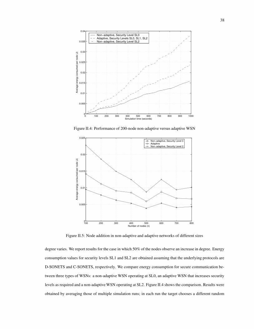
38

0 100 200 300 400 500 600 700 800 900 10000

0.005

0.01

0.015

0.02

0.025

0.03

0.035

0.04

Simulation time (seconds)

Ave

rage

ene

rgy

cons

umed

per

nod

e (J

)

Non−adaptive, Security Level SL0Adaptive, Security Levels SL0, SL1, SL2Non−adaptive, Security Level SL2

Figure II.4: Performance of 200-node non-adaptive versus adaptive WSN

100 200 300 400 500 600 700 8000

0.005

0.01

0.015

0.02

0.025

Number of nodes (n)

Ave

rage

ene

rgy

cons

umed

per

nod

e (J

)

Non−adaptive, Security Level 0AdaptiveNon−adaptive, Security Level 2

Figure II.5: Node addition in non-adaptive and adaptive networks of different sizes

degree varies. We report results for the case in which 50% of the nodes observe an increase in degree. Energy

consumption values for security levels SL1 and SL2 are obtained assuming that the underlying protocols are

D-SONETS and C-SONETS, respectively. We compare energy consumption for secure communication be-

tween three types of WSNs: a non-adaptive WSN operating at SL0, an adaptive WSN that increases security

levels as required and a non-adaptive WSN operating at SL2. Figure II.4 shows the comparison. Results were

obtained by averaging those of multiple simulation runs; in each run the target chooses a different random

39

path of movement through the network, thus causing different nodes operating at higher security levels to

expend energy for secure communication. We observe that results are as expected and indicate that energy

can be saved by allowing nodes to adapt themselves to changes and choose the appropriate security level as

opposed to employing the highest security level continuously. The overall energy consumed by nodes in an

adaptive WSN is approximately 38% less than those in a non-adaptive WSN operating at SL2 continuously.

Similarly, the overall energy consumption of an adaptive WSN is approximately 22.5% greater than that of a

non-adaptive WSN operating at SL0 continuously. We observe that transitioning between SL0, SL1 and SL2

provides an acceptable trade-off between security and energy consumption in a WSN under a potential node

addition attack. If all nodes successfully join the existing WSN at SL2, each node that observed an increase

in its degree updates it to the new value and uses it for all subsequent determinations of security state. At this

point, security level can be dropped to SL0. A WSN can accomplish this task easily using SWANS, because

after a successful join operation by new nodes, each affected node’s state returns to “Normal”, thus triggering

a Drop Security Level action.

In order to show that SWANS is scalable with respect to network size, we simulated networks of sizes

ranging from 100 to 800 nodes, 1% of which were RRNs. Figure II.5 shows the average energy consumed

per node for different network sizes and adaptive capabilities. We observe that energy consumption initially

decreases with increasing network size and becomes flat except when n=600. We have verified that the

deviation observed at this point is due to the nature of the random topologies of 600-node networks generated

by the simulator. The initial decrease can be attributed to the fact that nodes require fewer hops to reach a

base station in larger networks than smaller ones because the former have more base stations than the latter

[2]. However, once the hop counts stabilize, energy consumption becomes flat.

II.H.4 Thresholds for Node Addition

In this experiment, we are interested in answering the following question: What is an acceptable increase in

a node’s degree when network size increases by a fixed number of nodes, H ? By answering this question, we

can determine accurate values of two bounds n1 and n2 that govern the quantum of increase in node degree,

for any network whose size increases by n nodes. We choose H��[)\* in this experiment.

Network sizes range between 200 and 390 nodes, with the number of RRNs remaining at 2. The size

of each network is increased by 10 nodes. Table II.17 shows the results of this simulation. The first two

columns show original and final network sizes. As the results indicate, the mean increase in node degree

40

Orig. WSN New WSN �#]Y^\_ �']Y^+_ �!]Y^+_+� Size Size ���&]Y^\_200 210 0.78 0.87 2.52 0.020210 220 0.84 0.90 2.64 0.015220 230 0.57 0.65 1.87 0.023230 240 0.65 0.86 2.37 0.023240 250 0.79 0.96 2.66 0.015250 260 0.70 0.63 1.96 0.003260 270 0.78 0.87 2.53 0.017270 280 0.64 0.86 2.37 0.020280 290 0.66 0.78 2.23 0.023290 300 0.72 0.96 2.64 0.022300 310 0.74 0.84 2.43 0.019310 320 0.75 0.91 2.57 0.023320 330 0.75 0.64 2.03 0.023330 340 0.66 0.79 2.24 0.021340 350 0.52 0.79 2.12 0.023350 360 0.55 0.68 1.91 0.023360 370 0.72 0.72 2.15 0.022370 380 0.63 0.71 2.06 0.022380 390 0.55 0.82 2.19 0.021390 400 0.75 0.83 2.41 0.023

Table II.17: Increase in node degree (�`���

) for various network sizes

( �!]Y^\_ ) is 1 (rounding-up fractions greater than 0.5) for all network sizes. The standard deviation ( �!]Y^\_ ) of

the distribution of differences in node degree for each case, shown in column four of the table, indicates that

the width of the distribution is significantly high. We have observed that the tail of the distribution of values

greater than the mean is long, whereas that of values less than the mean is short. The maximum�����

ranges

between 2 and 5 nodes. We map the distribution of increases in node degree to a normal distribution and

assume that all increases greater than two standard deviations away from the mean, i.e., a ] ^+_b����� ] ^\_ in

Table II.17 should trigger a change in security levels. Under this assumption, the probability that a transition

to security level SL2 will be triggered is between 0.015 and 0.023, as shown in the last column of Table II.17.

Based on increases in node degree shown in Table II.17, a WSN designer can choose one of the following

two pairs of values for n1 and n2, respectively: (1,3) or (2,4). Thus, using the first pair of values for n1 and

n2, a node can be in the following states: NORMAL, as long as node degree increases by 1; HIGH if node

degree increases by 2 or 3; ABNORMAL HIGH if it increases by more than 3. Therefore, when a node’s

degree increases by 2 or 3, its security level changes from SL0 to SL1, and from SL1 to SL2 when degree

increases by more than 3. A similar analysis can be performed when HY) �c� and H#�d��e .In order to determine the best pair of values to use for HY) and H#� when network size increases by 10

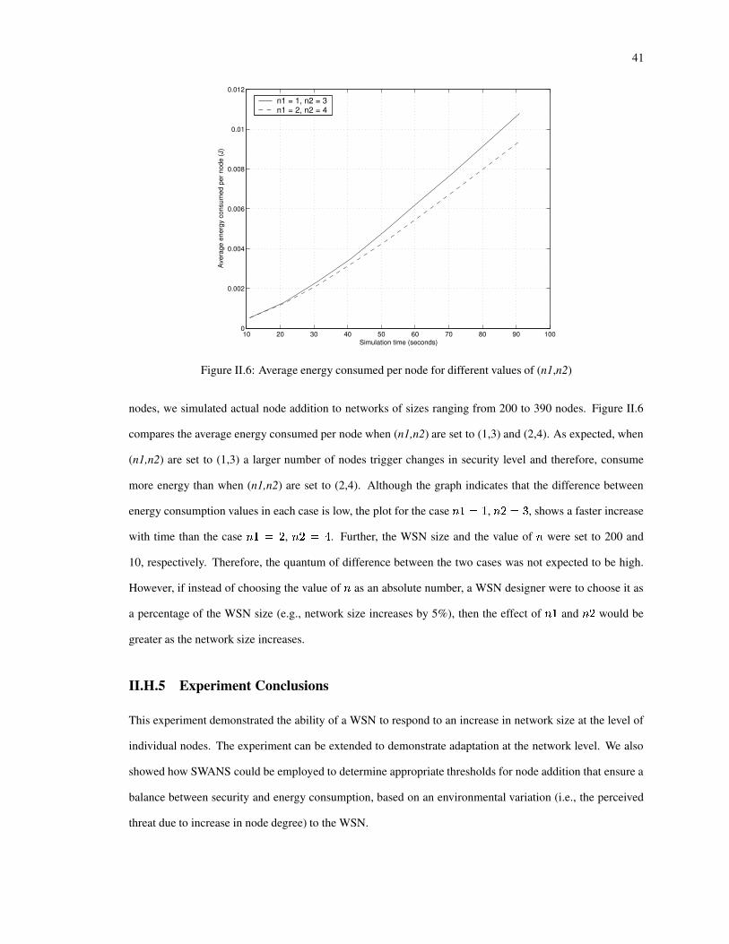
41

10 20 30 40 50 60 70 80 90 1000

0.002

0.004

0.006

0.008

0.01

0.012

Simulation time (seconds)

Ave

rage

ene

rgy

cons

umed

per

nod

e (J

)

n1 = 1, n2 = 3n1 = 2, n2 = 4

Figure II.6: Average energy consumed per node for different values of (n1,n2)

nodes, we simulated actual node addition to networks of sizes ranging from 200 to 390 nodes. Figure II.6

compares the average energy consumed per node when (n1,n2) are set to (1,3) and (2,4). As expected, when

(n1,n2) are set to (1,3) a larger number of nodes trigger changes in security level and therefore, consume

more energy than when (n1,n2) are set to (2,4). Although the graph indicates that the difference between

energy consumption values in each case is low, the plot for the case HY) �f) , H#�d�Zg , shows a faster increase

with time than the case HY)��h� , H#�F�ie . Further, the WSN size and the value of H were set to 200 and

10, respectively. Therefore, the quantum of difference between the two cases was not expected to be high.

However, if instead of choosing the value of H as an absolute number, a WSN designer were to choose it as

a percentage of the WSN size (e.g., network size increases by 5%), then the effect of HY) and H#� would be

greater as the network size increases.

II.H.5 Experiment Conclusions

This experiment demonstrated the ability of a WSN to respond to an increase in network size at the level of

individual nodes. The experiment can be extended to demonstrate adaptation at the network level. We also

showed how SWANS could be employed to determine appropriate thresholds for node addition that ensure a

balance between security and energy consumption, based on an environmental variation (i.e., the perceived

threat due to increase in node degree) to the WSN.

42

II.I Adaptability to Sleep Deprivation Torture Attack (SDTA)

In this experiment, we evaluate a WSN’s ability to detect a sleep deprivation torture attack (SDTA) [56] and

adapt to it in order to conserve energy. Therefore, the metric of interest in this case is longevity.

II.I.1 SDTA

Stajano and Anderson [56] suggest that legitimate nodes in a wireless ad hoc network are susceptible to

SDTA. In SDTA, legitimate nodes unknowingly interact with malicious nodes and in the process consume

valuable battery power. The interactions are designed to appear legitimate, but in reality are one of many

mechanisms to ensure the death of nodes. The unattended nature of WSNs renders them more susceptible to

SDTA than wireless ad hoc networks in which devices could be under user control. Stajano and Anderson

point out that one of the many defenses against SDTA is for nodes to become “unresponsive” and indicate

that such a defense would be counterproductive in ad hoc networks. They discuss a solution called the

“resurrecting duckling” to solve SDTA at higher layers of the network stack.

Malicious nodes can launch a SDTA against legitimate nodes at the routing, MAC and PHY layers of the

networking stack, and also at the application layer. In this experimental evaluation, we focus on SDTA at

the PHY and MAC layers as solutions to this problem at higher layers, such as resurrecting duckling, exist.

Malicious activity at the MAC and PHY layers could be harder to detect than at higher layers due to other

factors such as noise in the environment or high node density.

II.I.2 Defending Against SDTA Using SWANS

A WSN can detect SDTA at the MAC and PHY layers, and adapt to it using SWANS. Four parameters, shown

in Table II.1, are useful in indicating SDTA: FCS Failure Rate (FFR) and Collision Ratio (CR) at the MAC

layer, and HEC Failure Rate (HFR) and Format Violation Ratio (FVR) at the PHY layer. In SWANS, the

main defense against SDTA is that each individual node goes into a passive or sleep state (as opposed to an

unresponsive state) from which it can be woken up by a broadcast from a resource rich node. Schurgers et

al. [52] suggest the inclusion of a low-power radio on each sensor node which would only be used to wake

up sleeping nodes, thereby ensuring that the primary radio used for data communication maybe completely

turned off to conserve energy. Therefore, nodes in a WSN can adapt to SDTA by employing a dual-radio,

monitoring MAC and PHY parameters, and waking up once the attack has passed or upon instruction from a

43

Parameter Mean Std. Dev.FFR 0.1 0.05CR 0.25 0.1

HFR 0.12 0.04FVR 0.12 0.04

Table II.18: Values to Compute Parameter Thresholds

RRN.

In order to trigger the detection of SDTA at the MAC and PHY layers using FFR, CR, HFR and FVR, each

parameter must be associated with a set of lower and upper bounds. We accomplish this task by simulating

WSNs of different sizes and capturing values of these four parameters over a fixed time period as nodes in the

WSN communicate with each other. We compute the mean and variance of the data distribution associated

with each parameter, which we employ in establishing thresholds. We observed initially that both HFR and

FVR were 0 at the end of each simulation, i.e., no HEC failures or format violations were recorded. Therefore,

in order to set up non-zero thresholds, we used a random walk generator to simulate HEC failures and format

violations during normal communications between sensor nodes, and computed mean and variance of the

data distributions for HFR and FVR. After computing the mean and variance, thresholds for each parameter

are calculated using Tables II.5 and II.4.

II.I.3 Results

This experiment was designed to evaluate both node-level and network-level adaptability. We discuss them

separately in the sections below. Table II.18 shows the mean and standard deviation values obtained using

procedures discussed in Section II.I.2 and employed in this experiment.

Node-level Adaptability to SDTA

We simulated WSNs whose sizes ranged from 100 nodes to 800 nodes. Each simulated WSN is initialized

with threshold values for FFR, CR, HFR and FVR as described above. A mobile target node begins to

travel within the area of deployment (see Table II.17) and periodically emits a signal. Nodes in its vicinity

communicate with neighbors as they detect the target. Because the J-Sim simulator does not allow nodes to

be added to a network after the simulation is started, SDTA must be simulated on each individual node. This

is done by ensuring that values of one or more of the four monitored parameters crosses the prescribed upper

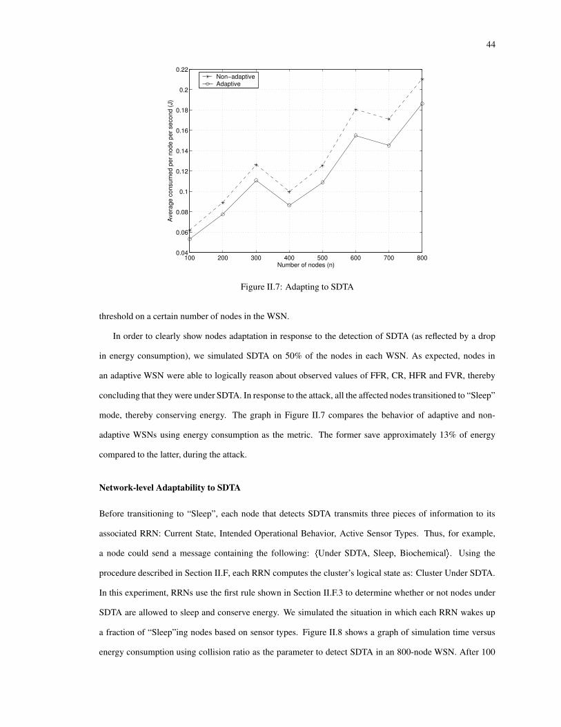
44

100 200 300 400 500 600 700 8000.04

0.06

0.08

0.1

0.12

0.14

0.16

0.18

0.2

0.22

Number of nodes (n)

Ave

rage

con

sum

ed p

er n

ode

per s

econ

d (J

)

Non−adaptiveAdaptive

Figure II.7: Adapting to SDTA

threshold on a certain number of nodes in the WSN.

In order to clearly show nodes adaptation in response to the detection of SDTA (as reflected by a drop

in energy consumption), we simulated SDTA on 50% of the nodes in each WSN. As expected, nodes in

an adaptive WSN were able to logically reason about observed values of FFR, CR, HFR and FVR, thereby

concluding that they were under SDTA. In response to the attack, all the affected nodes transitioned to “Sleep”

mode, thereby conserving energy. The graph in Figure II.7 compares the behavior of adaptive and non-

adaptive WSNs using energy consumption as the metric. The former save approximately 13% of energy

compared to the latter, during the attack.

Network-level Adaptability to SDTA

Before transitioning to “Sleep”, each node that detects SDTA transmits three pieces of information to its

associated RRN: Current State, Intended Operational Behavior, Active Sensor Types. Thus, for example,

a node could send a message containing the following: P Under SDTA, Sleep, Biochemical j . Using the

procedure described in Section II.F, each RRN computes the cluster’s logical state as: Cluster Under SDTA.

In this experiment, RRNs use the first rule shown in Section II.F.3 to determine whether or not nodes under

SDTA are allowed to sleep and conserve energy. We simulated the situation in which each RRN wakes up

a fraction of “Sleep”ing nodes based on sensor types. Figure II.8 shows a graph of simulation time versus

energy consumption using collision ratio as the parameter to detect SDTA in an 800-node WSN. After 100

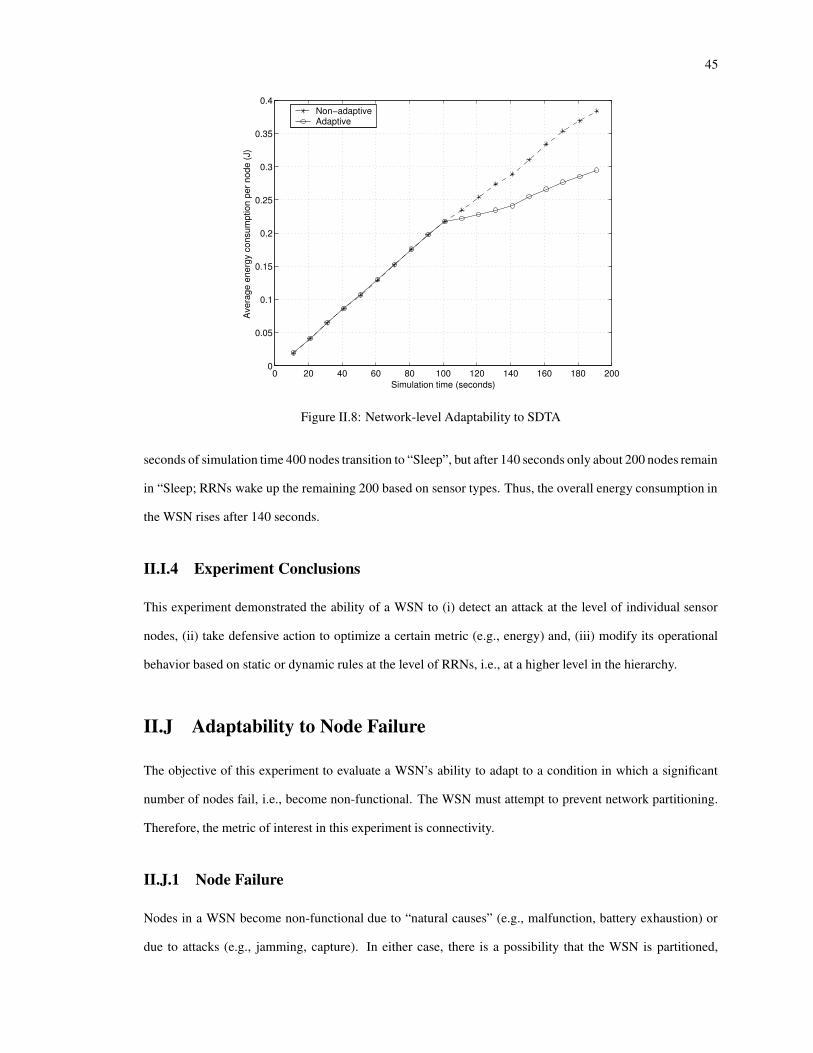
45

0 20 40 60 80 100 120 140 160 180 2000

0.05

0.1

0.15

0.2

0.25

0.3

0.35

0.4

Simulation time (seconds)

Ave

rage

ene

rgy

cons

umpt

ion

per n

ode

(J)

Non−adaptiveAdaptive

Figure II.8: Network-level Adaptability to SDTA

seconds of simulation time 400 nodes transition to “Sleep”, but after 140 seconds only about 200 nodes remain

in “Sleep; RRNs wake up the remaining 200 based on sensor types. Thus, the overall energy consumption in

the WSN rises after 140 seconds.

II.I.4 Experiment Conclusions

This experiment demonstrated the ability of a WSN to (i) detect an attack at the level of individual sensor

nodes, (ii) take defensive action to optimize a certain metric (e.g., energy) and, (iii) modify its operational

behavior based on static or dynamic rules at the level of RRNs, i.e., at a higher level in the hierarchy.

II.J Adaptability to Node Failure

The objective of this experiment to evaluate a WSN’s ability to adapt to a condition in which a significant

number of nodes fail, i.e., become non-functional. The WSN must attempt to prevent network partitioning.

Therefore, the metric of interest in this experiment is connectivity.

II.J.1 Node Failure

Nodes in a WSN become non-functional due to “natural causes” (e.g., malfunction, battery exhaustion) or

due to attacks (e.g., jamming, capture). In either case, there is a possibility that the WSN is partitioned,

46

100 200 300 400 500 600 700 8000.03

0.04

0.05

0.06

0.07

0.08

0.09

0.1

0.11

0.12

Number of nodes (n)

Avg

. ene

rgy

cons

umed

per

nod

e pe

r sec

ond

(J)

Non−adaptiveAdaptive

Figure II.9: Cost of Adapting to Node Failure

causing groups of nodes to become unreachable from the rest of the network. Solutions to this problem

include (i) addition of new nodes in the vicinity of failed nodes and (ii) increasing the transmission range of

the affected nodes in order to maintain connectivity with the rest of the network. The first solution requires

human intervention, whereas the second solution can be implemented using tunable radios on sensor nodes

to transmit at higher power, thereby increasing their transmission range. However, the second solution may

lead to rapid reduction in overall energy in the network, rendering it a temporary solution.

II.J.2 SWANS Against Node Failure

In order to adapt to node failure, each node must be capable of detecting such a condition. SWANS provides

a routing layer parameter, Failed Neighbor (FN) count, computed as a fraction of the current Node Degree

(ND), to track the level of failures. Each node can employ routing layer mechanisms to determine whether

a neighbor is functional or not. For example, if an expected message acknowledgment from a neighbor is

not received even after repeated attempts, then a node labels the neighbor as “failed” and increments FN.

Fraction k , that tracks the fraction of failed neighbors and shown in Table II.7, is a user-defined value. k must

be chosen carefully, because a trade-off exists between energy consumption and the level of connectivity. If kis too low, then nodes may be required to increase transmission range after the failure of only a small number

of neighbors is detected, leading to higher energy consumption. If k is too high, then connectivity is affected

leading to higher loss of data.

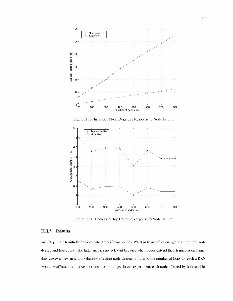
47

100 200 300 400 500 600 700 8000

20

40

60

80

100

120

Number of nodes (n)

Ave

rage

nod

e de

gree

(nd)

Non−adaptiveAdaptive

Figure II.10: Increased Node Degree in Response to Node Failure

100 200 300 400 500 600 700 8001.5

2

2.5

3

3.5

4

4.5

5

5.5

Number of nodes (n)

Ave

rage

hop

cou

nt to

RR

N

Non−adaptiveAdaptive

Figure II.11: Decreased Hop Count in Response to Node Failure

II.J.3 Results

We set kl�[*1Rnm�S initially and evaluate the performance of a WSN in terms of its energy consumption, node

degree and hop count. The latter metrics are relevant because when nodes extend their transmission range,

they discover new neighbors thereby affecting node degree. Similarly, the number of hops to reach a RRN

would be affected by increasing transmission range. In our experiment, each node affected by failure of its

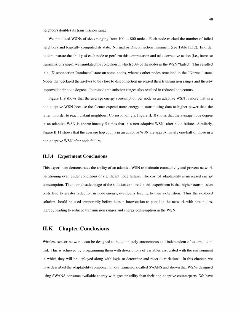
48

neighbors doubles its transmission range.

We simulated WSNs of sizes ranging from 100 to 800 nodes. Each node tracked the number of failed

neighbors and logically computed its state: Normal or Disconnection Imminent (see Table II.12). In order

to demonstrate the ability of each node to perform this computation and take corrective action (i.e., increase

transmission range), we simulated the condition in which 50% of the nodes in the WSN “failed”. This resulted

in a “Disconnection Imminent” state on some nodes, whereas other nodes remained in the “Normal” state.

Nodes that declared themselves to be close to disconnection increased their transmission ranges and thereby

improved their node degrees. Increased transmission ranges also resulted in reduced hop counts.

Figure II.9 shows that the average energy consumption per node in an adaptive WSN is more that in a

non-adaptive WSN because the former expend more energy in transmitting data at higher power than the

latter, in order to reach distant neighbors. Correspondingly, Figure II.10 shows that the average node degree

in an adaptive WSN is approximately 5 times that in a non-adaptive WSN, after node failure. Similarly,

Figure II.11 shows that the average hop counts in an adaptive WSN are approximately one-half of those in a

non-adaptive WSN after node failure.

II.J.4 Experiment Conclusions

This experiment demonstrates the ability of an adaptive WSN to maintain connectivity and prevent network

partitioning even under conditions of significant node failure. The cost of adaptability is increased energy

consumption. The main disadvantage of the solution explored in this experiment is that higher transmission

costs lead to greater reduction in node energy, eventually leading to their exhaustion. Thus the explored

solution should be used temporarily before human intervention to populate the network with new nodes,

thereby leading to reduced transmission ranges and energy consumption in the WSN.

II.K Chapter Conclusions

Wireless sensor networks can be designed to be completely autonomous and independent of external con-

trol. This is achieved by programming them with descriptions of variables associated with the environment

in which they will be deployed along with logic to determine and react to variations. In this chapter, we

have described the adaptability component in our framework called SWANS and shown that WSNs designed

using SWANS consume available energy with greater utility than their non-adaptive counterparts. We have

49

also shown that SWANS is scalable with respect to network size and can be used to enable both resource-

constrained and resource-rich nodes adaptive. SWANS also enables a sensor network designer to create

environmental descriptions of different complexities and validate them offline prior to actual deployment on

sensor nodes.

Chapter III

P-SONETS: SECURE WIRELESS SENSOR

NETWORKS FOR PERIMETER PROTECTION

III.A Introduction

In this chapter we motivate the need to build security as a core component of heterogeneous wireless sensor

networks using the class of perimeter protection applications as the driver. We identify threats and vulner-

abilities to WSNs deployed for perimeter protection, starting from the radio layer and progressing to the

application layer. We describe a centralized security model that serves as a countermeasure to the identified

threats. Our model utilizes a trusted base station to establish a secure perimeter around the chosen asset using

sensor nodes consisting of one or more sensor interfaces. We have implemented our model in SensorSim [46]

and evaluated its performance in terms of energy consumption and ability to detect malicious behavior in the

network to prevent a breach in the perimeter.

III.B Perimeter Protection

The following example describes a scenario that requires a secure perimeter capable of handling multiple

threats:

In today’s geopolitical climate the threat posed to high-level government officials is overwhelming, par-

ticularly when they are engaged in official business and traveling outside their home countries.

50

51

Consider the typical case of a country’s foreign minister. She travels extensively, often on the spur of the

moment, and sometimes to destinations that are hostile. Due to the nature of her office, her security detail

may not have had adequate time to conduct a detailed advance and install the requisite security controls.

The foreign minister faces a number of threats. Physical threats include poisoning from radiation, chemi-

cal or biological toxins. These are in addition to threats from explosives and individuals utilizing small arms

or other military ordinance. More insidious threats are posed by collection efforts aimed at both the substance

of her agenda and at analyzing security controls in order to compromise them at some later time.

Such perimeter security applications represent a vast class of “monitoring and responding” type applica-

tions for which heterogeneous WSNs will be deployed. We believe that a solution designed to mitigate the

aforementioned threats will also cover the broad spectrum of all threat models that such applications face.

The application scenario described above and its attendant security model may be abstracted and applied

to other scenarios where concentric circles of perimeter protection need to be temporarily established. Ex-

amples of other applications are placing alarm fields on a border and at ports of entry in order to prevent the

smuggling of hazardous materials and munitions and to prevent illegal entry. For example, suppose informa-

tion is developed leading to the suspicion that some person or persons unknown will be attempting to move

fissionable material across a remote section of a country’s border. Furthermore, suppose that this material

produces a signature which is only discernible at distances of 20 meters or less. Such a scenario is within

the realm of possibility. Moreover, it is conceivable that those behind such an operation could be leaking

spurious information so as to cause the authorities to take precautionary measures, only to study, analyze and

circumvent future preventive measures. This is in effect a “dry run” in preparation for the actual event. A

heterogeneous WSN could be rapidly deployed in order to prevent and apprehend those involved in such an

event. However, the underlying architecture of the WSN must be able to withstand probes and analyses in

order to remain effective over time.

III.B.1 Sensor Technology as a Solution

Sensor technologies have matured sufficiently over the years to miniaturize sensor types such as accelerom-

eters, microphones, light and motion detectors, and magnetometers. We envision a WSN design inclusive of

these sensors types; however, our application assumes a (not so) futuristic scenario that include sensors that

test for nitrates (explosives), chemical toxins, biological toxins and radiation. For example, sensors testing

for motion and sound would be placed on rooftops to detect the presence of assailant(s). Sensors testing

52

for radiation would be placed in areas frequented by the protectee, while sensors testing for chemical and

biological toxins would be placed in airways that feed into areas frequented by the protectee. Our colleagues

at UMBC in the Department of Chemical and Biochemical Engineering are deploying such sensors [33], and

we feel that such sensors will eventually be integrated with sensor prototypes.

III.B.2 Securing Wireless Sensor Networks

Our contribution in this area is the creation of lightweight techniques for securing existing sensor network

routing and data movement approaches, such as directed diffusion [26], SPIN [35] and data dissemination

[8, 38]. We assume the computational capability and memory requirements typical of those provided by

sensor nodes designed for the applications described above. We further assume that the base station is fixed,

always attended and is in a secure location. We make no attempt to counter the threat from a widespread

denial of service attack against the RF layer. As pointed out in [48], such attacks are fairly straightforward

to mount against fixed frequency RF communication links that are found in the sensors. Defending against

them requires changes to the RF layer of the sensor, such as the use of spread spectrum techniques, which

can mitigate against an RF level DoS attack. In our scenario, and many others, a denial of service is in itself

an alarm.

III.B.3 Threat Model

We model threats against a WSN deployed for perimeter protection in terms of the following actions that an

adversary may take into order to disrupt it and breach the perimeter.

i. Passive Information Gathering: If communications between sensor nodes or between sensor nodes and

the base station are in the clear, then an adversary with an appropriately powerful receiver and well

designed antenna can easily read off the data stream. Further, if routing messages containing source

and destination addresses are transmitted without encryption, then the adversary can analyze messages

to eventually learn the entire topology and subsequently subvert the network. We employ the term

traffic analysis to describe this threat.

ii. Node Compromise: The adversary can physically capture a node and compromise it. Node compromise

includes extracting secret information from the node and deploying malicious code on it such that the

node misbehaves during interactions with other nodes.

53

iii. False Node: An intruder can add malicious nodes to the WSN that feed false data or prevent the

passage of true data. Malicious nodes could also force legitimate nodes to continuously engage in

energy consuming communications and computations leading to network failure.

III.C Background

Relatively few security protocols described in current literature employ a base station model for wireless

sensor networks. In this section, we describe a few security protocols for WSNs that employ a base station

model.

Perrig et al. [48] describe “SPINS: Security Protocols for Sensor Networks” comprised of Sensor Network

Encryption Protocol (SNEP) and � TESLA. The function of SNEP is to provide confidentiality (privacy), two-

party data authentication, integrity and freshness. � TESLA is to provide authentication to data broadcasts.

SPINS presents an architecture where the base station accesses nodes using source routing. We describe

SPINS in greater detail in Section III.E.4 and also compare it to our model.

Carman et al. [10] have conducted a detailed study of various keying protocols applicable to distributed

sensor networks. They classify these protocols under pre-deployed keying, arbitrated protocols, self-enforcing

autonomous keying protocols and hybrid approaches. The authors also present detailed comparisons between

various keying protocols in terms of energy consumption.

III.D Wireless Sensor Network Model

The model of the WSN deployed for perimeter protection is discussed in the following points:

� The base station is computationally robust, having the requisite processor speed, memory and power

to support cryptographic and routing requirements of the sensor network. As stated above, the base

station is in a fixed, secure location and is always attended. Hence, it is considered to be within a

trusted computing environment. The assumptions of secure location and constant attendance are not

valid for the individual sensor nodes.

� Key management and re-keying mechanisms are not necessary because the base station, which holds

the cryptographic keys of all sensor nodes, is secure.

54

BS

Figure III.1: Example Network Topology

� The communication paradigm is one-to-one, not one-to-many or many-to-one. Even though all mes-

sages are broadcast at the routing and MAC levels, each message has an intended recipient. The threat

of traffic analysis is mitigated by the encryption of addresses.

� The physical security protocol of our application class follows the traditional model of concentric

circles of protection, where the the inner circle is resource rich. Conversely, as the distance from the

inner circle increases, the controls and mechanism become more general and are deployed in fewer

numbers.

III.E Security Model

Security is a broadly used term encompassing the characteristics of authentication, integrity, confidentiality,

non-repudiation and anti-playback. In the case of our WSN, security requirements are comprised of au-

thentication, integrity, confidentiality, anti-playback and resilience against traffic analysis. The recipient of a

message must be able to be unequivocally assured that the message came from its stated source. Similarly,

the recipient must be assured that the message was not altered in transit and that it is not an earlier message

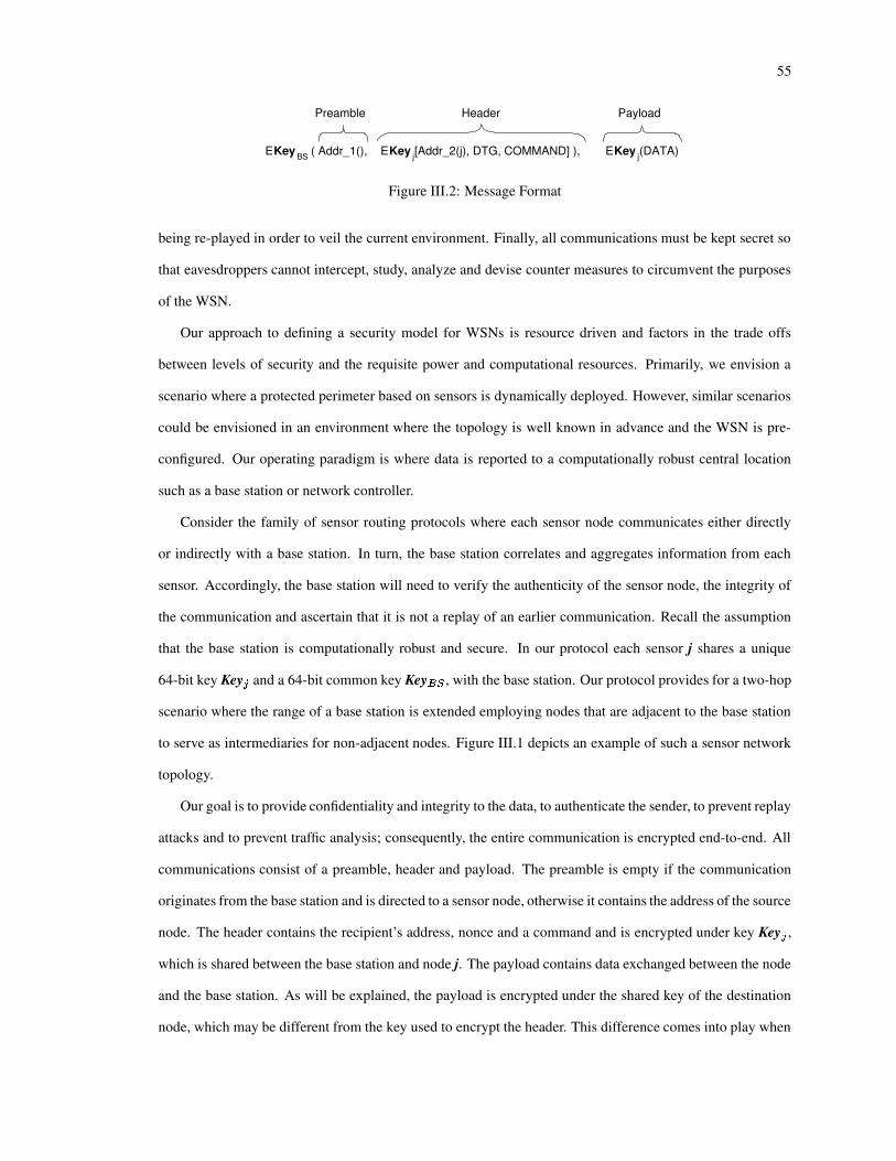
55

E Key BS ( Addr_1(), E Key j [Addr_2(j), DTG, COMMAND] ),

Preamble Header Payload

E Key j (DATA)

Figure III.2: Message Format

being re-played in order to veil the current environment. Finally, all communications must be kept secret so

that eavesdroppers cannot intercept, study, analyze and devise counter measures to circumvent the purposes

of the WSN.

Our approach to defining a security model for WSNs is resource driven and factors in the trade offs

between levels of security and the requisite power and computational resources. Primarily, we envision a

scenario where a protected perimeter based on sensors is dynamically deployed. However, similar scenarios

could be envisioned in an environment where the topology is well known in advance and the WSN is pre-

configured. Our operating paradigm is where data is reported to a computationally robust central location

such as a base station or network controller.

Consider the family of sensor routing protocols where each sensor node communicates either directly

or indirectly with a base station. In turn, the base station correlates and aggregates information from each

sensor. Accordingly, the base station will need to verify the authenticity of the sensor node, the integrity of

the communication and ascertain that it is not a replay of an earlier communication. Recall the assumption

that the base station is computationally robust and secure. In our protocol each sensor j shares a unique

64-bit key Key o and a 64-bit common key Key prq , with the base station. Our protocol provides for a two-hop

scenario where the range of a base station is extended employing nodes that are adjacent to the base station

to serve as intermediaries for non-adjacent nodes. Figure III.1 depicts an example of such a sensor network

topology.

Our goal is to provide confidentiality and integrity to the data, to authenticate the sender, to prevent replay

attacks and to prevent traffic analysis; consequently, the entire communication is encrypted end-to-end. All

communications consist of a preamble, header and payload. The preamble is empty if the communication

originates from the base station and is directed to a sensor node, otherwise it contains the address of the source

node. The header contains the recipient’s address, nonce and a command and is encrypted under key Key o ,which is shared between the base station and node j. The payload contains data exchanged between the node

and the base station. As will be explained, the payload is encrypted under the shared key of the destination

node, which may be different from the key used to encrypt the header. This difference comes into play when

56

the communication needs to be relayed by an intermediate node. Figure III.2 depicts the communication

format. The following rules apply to the use of the message format shown in the figure:

� Addr 1 is empty if the communication is from the base station to a sensor node.

� Addr 1 contains the address of the transmitting node if the communication is directed to the base

station. A non-empty Addr 1 field enables the base station to immediately select the correct key,

instead of trying keys until it locates the correct one.

� Addr 2 contains the address of the destination node if the communication is from the base station to a

node. If the communication is from a node to the base station Addr 2 will contain the address of the

source node.

� DTG is the date-time-group and is a nonce used to prevent replay attacks.

� COMMAND describes the contents of the message to the recipient.

Accordingly, a communication from the base station to a node j is of the form depicted in Figure III.2,

and a communication from a node j to the base station is of the form: E slt+u p6q (Preamble, E s�t+u o (Header)),

E slt+u o (Payload). On receipt, the base station decrypts the communication, uses the address contained in the

preamble to select the key shared with the node and decrypts the message.

The use of double encryption prevents the disclosure of node addresses, consequently preventing traffic

analysis. However, by listening to transmissions from nodes, an adversary would be able to determine the

number of nodes in the network. Should a single node be compromised and the its keys disclosed, the network

will be able to function albeit the unique addresses of each node will be disclosed.

III.E.1 Topology Discovery and Network Setup

The base station is deployed with the unique ID, symmetric encryption key of each node in the sensor network

and a master key, Key prq . Similarly, each node is deployed with the unique key, Key o that it shares with the

base station and Key prq . As in SPINS, its clock is synchronized with the base station’s clock. We note that

sensor nodes do not obtain their keys “over the air” from the base station; rather every node is programmed

with a unique key. Upon initialization of the sensor network, the base station learns the network topology,

creates and optimizes a routing table and provides a mechanism to non-adjacent (out of radio range) nodes

that enables them to securely communicate with the base station.

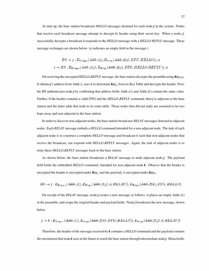
57

At start up, the base station broadcasts HELLO messages destined for each node j in the system. Nodes

that receive each broadcast message attempt to decrypt its header using their secret key. When a node, j,

successfully decrypts a broadcast it responds to the HELLO message with a HELLO-REPLY message. These

message exchanges are shown below. ( v indicates an empty field in the message.)

w<x�yhz|{�}b~b�����1�!�B� I>I@= ) ��� ? }b~b���G�@�B� I>I@= � ��zJ� ?G�����`?�� }d�������A� ?�vz:y�w<x�{�} ~b��� �1�/�B� I@I@= ) ��zJ� ? } ~b��� ���B� I>I@= � ��z>� ?G��� �`?G� }d����� ��}d�������G� ?DvOn receiving the encrypted HELLO REPLY message, the base station decrypts the preamble using Key prq .

It obtains j’s address from Addr 1, uses it to determine Key o from its Key Table and decrypts the header. First,

the BS authenticates node j by confirming that address fields Addr 1() and Addr 2() contain the same value.

Further, if the header contains a valid DTG and the HELLO REPLY command, then j is adjacent to the base

station and the latter adds that node to its route table. Those nodes that did not reply are assumed to be two

hops away and non-adjacent to the base station.

In order to discover non-adjacent nodes, the base station broadcasts RELAY messages directed to adjacent

nodes. Each RELAY message embeds a HELLO command intended for a non-adjacent node. The task of each

adjacent node is to construct a complete HELLO message and broadcast it such that non-adjacent nodes that

receive the broadcast, can respond with HELLO REPLY messages. Again, the task of adjacent nodes is to

relay these HELLO REPLY messages back to the base station.

As shown below, the base station broadcasts a RELAY message to node adjacent node j. The payload

field holds the embedded HELLO command, intended for non-adjacent node k. Observe that the header is

encrypted the header is encrypted under Key o and the payload, is encrypted under Key � .w<x�yhz|{�}b~b�����1�/��� I>I�= ) ��� ? }b~b���G����� I>I�= � ��zJ� ?�v�? ��}d�������G� ? }�~b�����1�B� I@I@= � � �1� ?������`?�� }d���¡���

On receipt of the RELAY message, node j creates a new message as follows: it places an empty Addr 1()

in the preamble, and swaps the original header and payload fields. Node j broadcasts the new message, shown

below.

z:y¢��{�} ~b��� �1�!�B� I>I@= ) ��� ? } ~b���D� �B� I>I@= � � �1� ?������`?G� }d���¡���A� ? } ~b��� �K�B� I@I@= � ��zJ� ?�v�? �£}������<�A�Therefore, the header of the message received by k contains a HELLO command and the payload contains

the mechanism that node k uses in the future to reach the base station through intermediate node j. Henceforth,

58

we refer to the mechanism, consisting of the intermediate node’s address and a RELAY command encrypted

under the intermediate node’s key, as ¤ .

To respond to the HELLO message from the BS, node k constructs a HELLO REPLY message as follows:

the preamble contains k, the header contains ¤ , and the payload contains k along with a DTG and the

HELLO REPLY command encrypted under Key � . This message is transmitted as shown below:

��yhz|{�}b~b�����1�!�B� I>I@= ) ���'� ?D¤ � ? }b~b���D�J��� I>I�= � ���'� ?G�|���`?G� }������ ��}d�����d�A�Node j receives the transmission, performs the outer decryption and attempts to decrypt the header (i.e.,

¤ ), using Key o . After successfully decrypting the header and noting the RELAY command, node j creates a

new message as follows: it places the original preamble in the new message’s preamble, places the original

payload in the header field and its own address encrypted under Key o in the payload field. Node j then

transmits it to the base station, as shown below:

z<y¢w<x�{�} ~b��� �1�/��� I>I�= ) ���'� ? } ~b����� �B� I>I@= � � �1� ?������`?G� }d���¡� ��}d�������A� ? } ~b��� ����zJ�The for steps described above are repeatedly executed until all non-adjacent nodes can reach the base

station via at least one adjacent node.

After discovering adjacent nodes and all of the paths by which non-adjacent nodes can reach it, the BS

optimizes its route table so as to not overburden an adjacent node with the task of relaying messages to and

from non-adjacent nodes. (Recall that each non-adjacent node has stored a mechanism ¤ that it uses to reach

the BS.) The optimization process may result in reassignment of a non-adjacent node to an adjacent node

different from that used to relay the HELLO REPLY message. In such a case, the base station sends the

non-adjacent node a new ¤ , containing the address of the new adjacent node.

The BS maintains three tables, shown in Figure III.3 to route instructions and help repair the network as

required. The Route Table contains the primary route, indicated by an *, and alternate routes to a node. An

entry of the form A:() indicates that the node is directly connected to the base station whereas an entry such

as D:(A) indicates that A is an intermediate node between the base station and node D.

The Key Table contains the unique key shared by node j and the base station. The Activity Table

contains the most recent Date Time Group (DTG) received by the base station from a particular node, a count

(Activity ¥ ) of corrupted messages sent by the node, and a count (Activity ¦ ) of route failures due to that

node. The values of Activity ¥ and Activity ¦ are used to detect aberrant behavior on the part of an individual

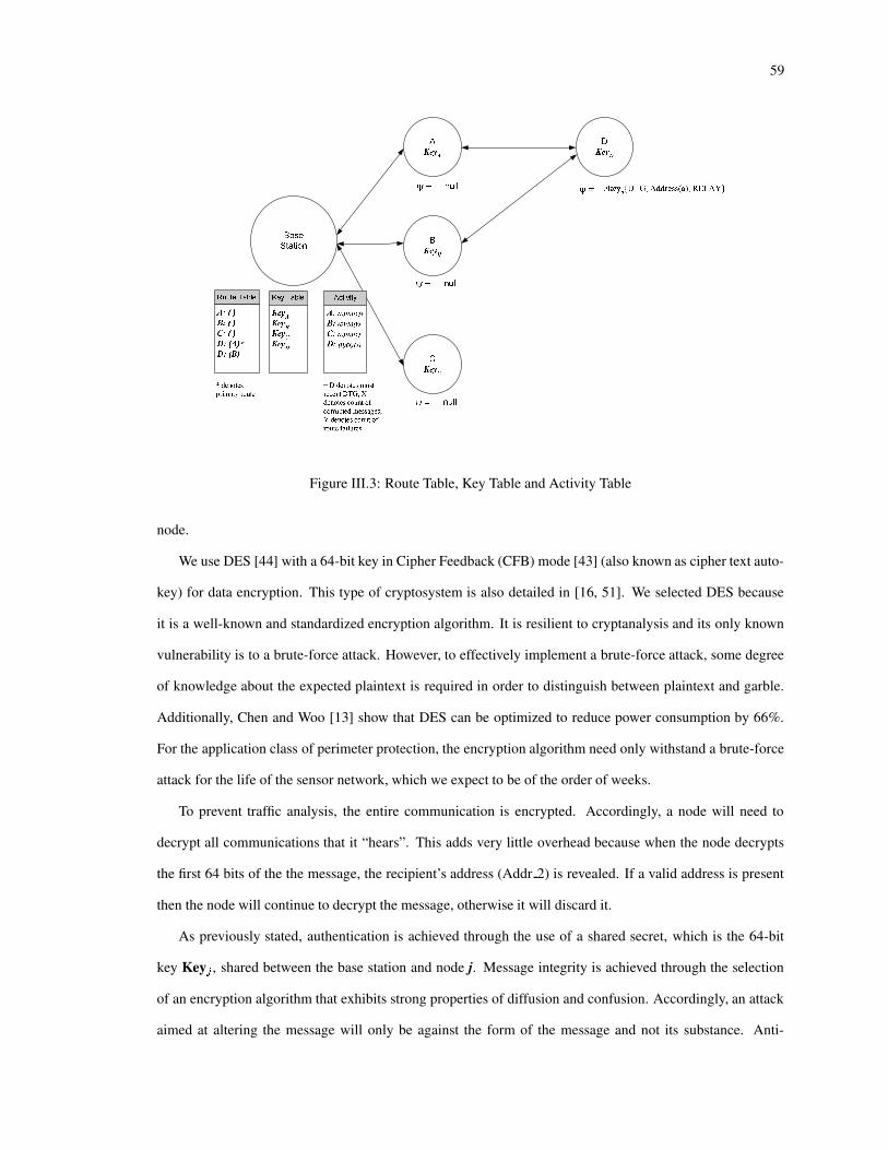
59

Figure III.3: Route Table, Key Table and Activity Table

node.

We use DES [44] with a 64-bit key in Cipher Feedback (CFB) mode [43] (also known as cipher text auto-

key) for data encryption. This type of cryptosystem is also detailed in [16, 51]. We selected DES because

it is a well-known and standardized encryption algorithm. It is resilient to cryptanalysis and its only known

vulnerability is to a brute-force attack. However, to effectively implement a brute-force attack, some degree

of knowledge about the expected plaintext is required in order to distinguish between plaintext and garble.

Additionally, Chen and Woo [13] show that DES can be optimized to reduce power consumption by 66%.

For the application class of perimeter protection, the encryption algorithm need only withstand a brute-force

attack for the life of the sensor network, which we expect to be of the order of weeks.

To prevent traffic analysis, the entire communication is encrypted. Accordingly, a node will need to

decrypt all communications that it “hears”. This adds very little overhead because when the node decrypts

the first 64 bits of the the message, the recipient’s address (Addr 2) is revealed. If a valid address is present

then the node will continue to decrypt the message, otherwise it will discard it.

As previously stated, authentication is achieved through the use of a shared secret, which is the 64-bit

key Key o , shared between the base station and node j. Message integrity is achieved through the selection

of an encryption algorithm that exhibits strong properties of diffusion and confusion. Accordingly, an attack

aimed at altering the message will only be against the form of the message and not its substance. Anti-

60

playback is achieved by the use the Date-Time-Group. Finally, privacy is achieved as a result of encrypting

all communications.

III.E.2 Inserting Additional Nodes into the Network

The insertion of additional nodes into the existing sensor network is easily accomplished. In our model the

unique identity and the key Key § of some node m to be added are loaded into the base station, the new node’s

clock is synchronized with that of the existing network and the base station repeats the topology discovery

algorithm, explicitly looking for the new node. Once the new node is discovered, the routing table is re-

optimized. For the perimeter protection application class, the need to insert additional nodes into the network

is not expected to be high, given the limited duration for which protection is required.

III.E.3 Isolating Aberrant Nodes

An aberrant node is one that is not functioning as specified. Identifying and isolating aberrant nodes that are

serving as intermediate nodes is important to the continued operation of the sensor network.

A node may cease to function as expected for several reasons:

1. It has exhausted its source of power.

2. It was damaged.

3. It is dependent upon an intermediate node and is being blocked because the intermediate node has

fallen victim to 1 and 2 above.

4. It is dependent upon an intermediate node and is being deliberately blocked because the intermediate

node has been compromised.

5. An intermediate node has been compromised and it is corrupting the communication by modifying data

before forwarding it.

Our protocol effectively mitigates against the class of attack/failure where an intermediate node is in-

volved. The protocol for the detection of aberrant nodes is presented in Figure III.4.

Periodically, the base station checks the activity table associated with a node, testing for a prolonged

period of inactivity,�

. If the node is directly connected (i.e., it does not rely upon an intermediate node) this

could be evidence of aberrant behavior on the part of the node. If the node relies upon an intermediate node

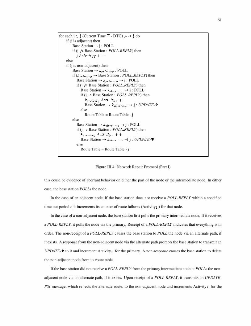
61

for each j ¨%© (Current Time � - DTG) 2 �«ª doif (j is adjacent) then

Base Stationy

j : POLLif (j ¬y Base Station : POLL-REPLY) then

j� ­ U�®°¯@®°U�u@¦%�3�

elseif (j is non-adjacent) then

Base Stationy±�K²´³Gµ § � ³�� : POLL

if (�¶²´³�µ § � ³�� y Base Station : POLL REPLY) thenBase Station

y±� ²·³�µ § � ³G� y j : POLLif (j ¬y Base Station : POLL REPLY) then

Base Stationy±� �D¸º¹ ��³ � �D¹ � y j : POLL

if (jy

Base Station : POLL REPLY) then� ²´³�µ § � ³�� � ­ U�®°¯@®°U�u ¦ �3�Base Station

y±� �D¸n¹ ��³ � �D¹ � y j : UPDATE- ¤else

Route Table = Route Table - jelse

Base Stationy±� �D¸n¹ ��³ � �D¹ �¡y j : POLL

if (jy

Base Station : POLL REPLY) then�K²´³Gµ § � ³G����­ U�®°¯>® U�u>¦%���Base Station

y±� �D¸º¹ ��³ � �D¹ ��y j : UPDATE- ¤else

Route Table = Route Table - j

Figure III.4: Network Repair Protocol (Part I)

this could be evidence of aberrant behavior on either the part of the node or the intermediate node. In either

case, the base station POLLs the node.

In the case of an adjacent node, if the base station does not receive a POLL-REPLY within a specified

time out period t, it increments its counter of route failures (Activity ¦ ) for that node.

In the case of a non-adjacent node, the base station first polls the primary intermediate node. If it receives

a POLL-REPLY, it polls the node via the primary. Receipt of a POLL-REPLY indicates that everything is in

order. The non-receipt of a POLL-REPLY causes the base station to POLL the node via an alternate path, if

it exists. A response from the non-adjacent node via the alternate path prompts the base station to transmit an

UPDATE- ¤ to it and increment Activity ¦ for the primary. A non-response causes the base station to delete

the non-adjacent node from its route table.

If the base station did not receive a POLL-REPLY from the primary intermediate node, it POLLs the non-

adjacent node via an alternate path, if it exists. Upon receipt of a POLL-REPLY, it transmits an UPDATE-

PSI message, which reflects the alternate route, to the non-adjacent node and increments Activity ¦ for the

62

for each j ¨ (� ­ U�®°¯@®°U�u@»c2�� C1=KtKX¶C'¼K½�I ) do

if (j is adjacent) thenfor each n ¨ Primary-Adjacent-List(j)

Base Stationy±� �D¸n¹ ��³ � �D¹ �¡y n : UPDATE- ¤

Route Table = Route Table - jelse

Base Stationy±� �D¸n¹ ��³ � ��¹ ��y j : POLL

if (j ¬y Base Station : POLL REPLY) thenRoute Table = Route Table - j

for each j ¨ Route Table doif (��­ U�® ¯>®°U�u ¦ 2��£C1=KtKX¶C'¼K½�I ) thenRoute Table = Route Table - j

Figure III.5: Network Repair Protocol (Part II)

primary. If it does not receive a POLL-REPLY from the non-adjacent node via the alternate path, it deletes

that node from its route table.

As shown in Figure III.5, the base station also checks for a high incidence of corrupted messages orig-

inating from a non-adjacent node. An intermediate node that has become aberrant may corrupt data that it

is relaying on behalf of a non-adjacent node. This behavior constitutes a denial-of-service (DoS) attack. In

order to mitigate against such an intermediate node, the base station keeps a counter of corrupted packets,

Activity ¥ . When this counter crosses a pre-determined threshold, the base station transmits an UPDATE- ¤to all non-adjacent nodes affected by the intermediate node via alternate paths, if they exist, and deletes the

aberrant intermediate node from its route table. A non-adjacent node may be sending corrupt data which the

intermediate faithfully relays. The base station tests for this situation by transmitting a POLL to the non-

adjacent node via an alternate path, if it exists. Non-receipt of a POLL-REPLY from the non-adjacent node

causes it to be deleted from the base station’s route table; receipt indicates that everything is in order. Finally,

nodes whose count of route failures, Activity ¦ , crosses the prescribed threshold are deleted from the Route

Table.

III.E.4 Comparison with SPINS

SPINS is comprised of Sensor Network Encryption Protocol (SNEP) and Micro Timed Efficient Stream Loss-

tolerant Authentication ( � TESLA). The function of SNEP is to provide confidentiality (privacy), two-party

data authentication, integrity and freshness. � TESLA is to provide authentication to data broadcasts. We

compare our security model to SNEP in terms of functionality. We do not compare it to � TESLA because

63

we do not perform broadcast authentication.

In SNEP each H!¼KI>t o shares a unique master key s o with the base station. This master key is used to

derive all other keys. For data encryption SNEP employs a one time encryption key produced by using

a key derived from s o and an incremental counter (message indicator) as inputs to the RC5 cryptographic

algorithm. The RC5 algorithm outputs a binary string that is used as the one time key. The message is XORed

with the one time key, transmitted and the counter is incremented in preparation for the next message. The

base station, aware of the node’s counter value and the derived key, produces the identical one time key,

XORs the encrypted message with the one time key to produce the clear text.

Our protocol differs from SPINS in the following fundamental and essential ways.

1. SPINS uses source routing, which like all non-broadcast routing mechanisms, is vulnerable to traffic

analysis. Our protocol relies upon broadcasts where the entire communication is end-to-end encrypted

in order to mitigate against the threat posed by traffic analysis.

2. We provide a mechanism for detecting certain types of aberrant behavior, behavior that may be due

to either a compromise or malfunction of an individual node. In either case we are able to remove

the node from the network. This is extremely important in the case of applications such as perimeter

protection, because the longer a compromised node remains in the network, the greater it’s chances of

being able to break down the perimeter.

3. SPINS has been highly optimized in order to reduce code footprint on the SmartDust Mote. Although

our model has not been optimized for a specific sensor platform, the encryption algorithm may be

replaced to better suit different hardware platforms.

In addition, we note that our protocol differs from SPINS in terms of the application class. Our protocol

is designed to function correctly in sensor networks used for perimeter protection.

III.F Experimental Evaluation

We have implemented the topology discovery and network setup components of our protocol using the Sen-

sorSim [46] extension of the NS network simulator [45]. The entire protocol, including cryptographic func-

tionality, is implemented at the routing layer. We generated 100 cryptographic keys, where the first key was

used as the Key p6q . These keys were placed in the base station. Individual keys and Key p6q were also placed

64

in each node. Topology distribution files, consisting of the (x,y) co-ordinates of each node were created for

four different distributions, which we explain shortly. Each distribution file and a configuration file were used

as inputs to the simulator. The correctness of the topology discovery and network setup protocol was verified

by observing the successful encryption, transmission, reception, decryption and response to each message.

Additionally, the routing table created by the base station was visually inspected to verify that each adjacent

node was associated with approximately the same number of non-adjacent nodes. The correctness of the

network repair protocol was verified by observing the base station’s response to node failures and corrupted

data.

III.F.1 Simulation

We used the simple battery, radio and CPU models of the simulator. According to the battery model, the

initial energy of the battery attached to each sensor node is 36 Asec (10 mAh). According to the radio

model, message transmission and reception at a data rate of 19.2 Kbps draw 5.2mA and 4.1mA of current,

respectively. The model assumes a radio range of 15m. The CPU model assumes that the CPU draws 2.9mA

in active mode and 1.9 mA in sleep mode. For purposes of this simulation, we assume a voltage of 1V. It

should be noted that the CPU is assumed to draw a constant amount of current in active mode, irrespective

of the task it performs, be it a simple arithmetic function or encryption of a message. We assume a message

length of either 24 or 48 bytes.

We conducted experiments to measure energy expenditure of each sensor function (Tx, Rx and CPU)

during network setup time for four different network topologies. We simulated a geographic environment

measuring 5654 m ¾ . We divided this environment into two concentric circles, the inner circle with a radius

of 15 meters and the outer circle with a radius of 30 meters. The base station was located at the center. The

sensor placement within our experimental topologies is as follows:

1. LIHO: 30 nodes randomly placed in the inner circle and 70 nodes randomly placed in the outer circle.

2. EIO: 50 nodes randomly placed in the inner circle and 50 nodes randomly placed in the outer circle.

3. HILO: 70 nodes randomly placed in the inner circle and 30 nodes randomly placed in the outer circle.

4. RND: 100 nodes randomly placed across the entire area.

The results of our experiments are illustrated in the graphs contained in Figures III.6–III.9. We measured

the energy consumed (Y axis) by each component of the sensor: the transmitter, receiver and CPU, for the

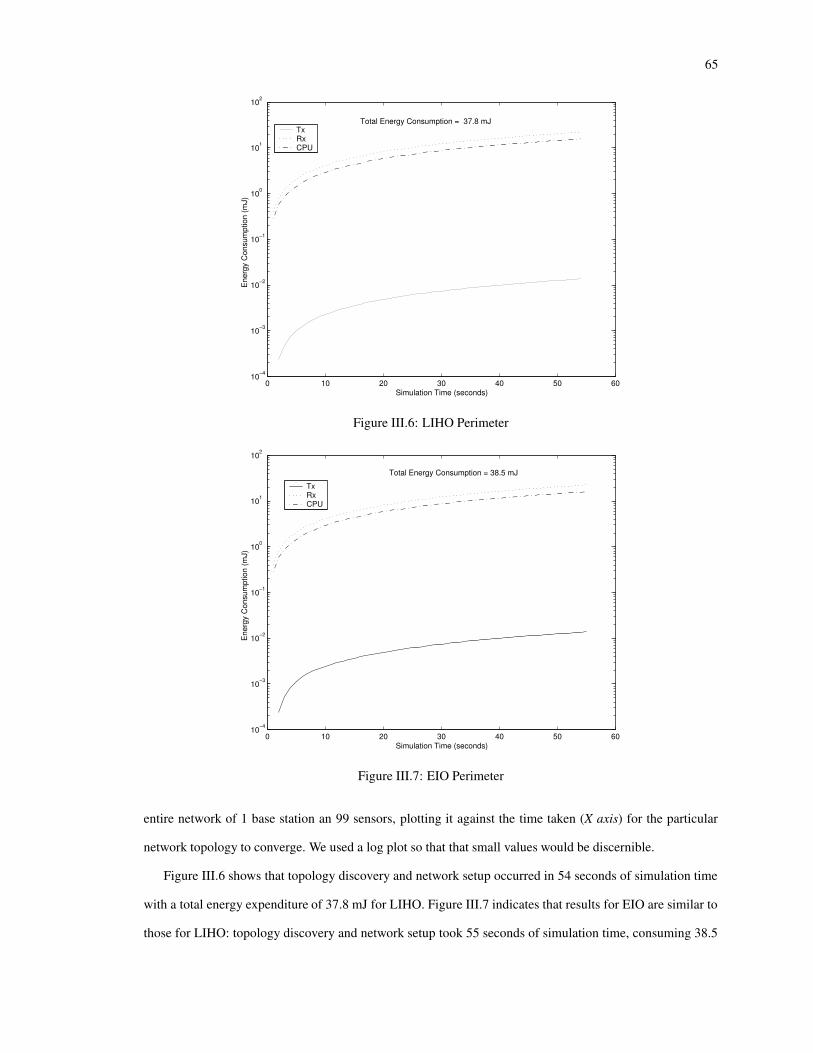
65

0 10 20 30 40 50 6010−4

10−3

10−2

10−1

100

101

102

Simulation Time (seconds)

Ene

rgy

Con

sum

ptio

n (m

J)

TxRxCPU

Total Energy Consumption = 37.8 mJ

Figure III.6: LIHO Perimeter

0 10 20 30 40 50 6010−4

10−3

10−2

10−1

100

101

102

Simulation Time (seconds)

Ene

rgy

Con

sum

ptio

n (m

J)

TxRxCPU

Total Energy Consumption = 38.5 mJ

Figure III.7: EIO Perimeter

entire network of 1 base station an 99 sensors, plotting it against the time taken (X axis) for the particular

network topology to converge. We used a log plot so that that small values would be discernible.

Figure III.6 shows that topology discovery and network setup occurred in 54 seconds of simulation time

with a total energy expenditure of 37.8 mJ for LIHO. Figure III.7 indicates that results for EIO are similar to

those for LIHO: topology discovery and network setup took 55 seconds of simulation time, consuming 38.5

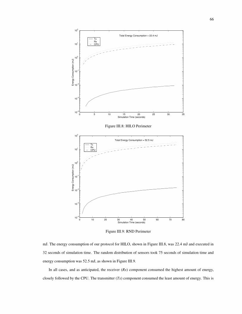
66

0 5 10 15 20 25 30 3510−4

10−3

10−2

10−1

100

101

102

Simulation Time (seconds)

Ene

rgy

Con

sum

ptio

n (m

J)

TxRxCPU

Total Energy Consumption = 22.4 mJ

Figure III.8: HILO Perimeter

0 10 20 30 40 50 60 70 8010−4

10−3

10−2

10−1

100

101

102

Simulation Time (seconds)

Ene

rgy

Con

sum

ptio

n (m

J)

TxRxCPU

Total Energy Consumption = 52.5 mJ

Figure III.9: RND Perimeter

mJ. The energy consumption of our protocol for HILO, shown in Figure III.8, was 22.4 mJ and executed in

32 seconds of simulation time. The random distribution of sensors took 75 seconds of simulation time and

energy consumption was 52.5 mJ, as shown in Figure III.9.

In all cases, and as anticipated, the receiver (Rx) component consumed the highest amount of energy,

closely followed by the CPU. The transmitter (Tx) component consumed the least amount of energy. This is

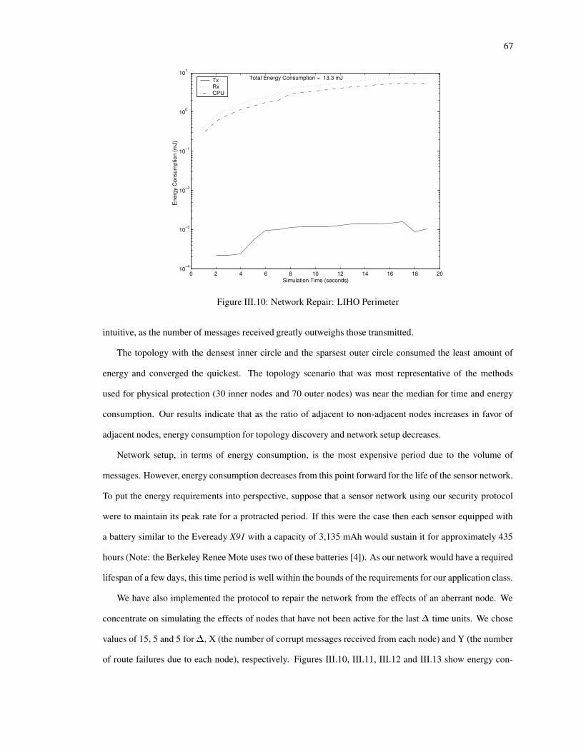
67

0 2 4 6 8 10 12 14 16 18 2010−4

10−3

10−2

10−1

100

101

Simulation Time (seconds)

Ene

rgy

Con

sum

ptio

n (m

J)

TxRxCPU

Total Energy Consumption = 13.3 mJ

Figure III.10: Network Repair: LIHO Perimeter

intuitive, as the number of messages received greatly outweighs those transmitted.

The topology with the densest inner circle and the sparsest outer circle consumed the least amount of

energy and converged the quickest. The topology scenario that was most representative of the methods

used for physical protection (30 inner nodes and 70 outer nodes) was near the median for time and energy

consumption. Our results indicate that as the ratio of adjacent to non-adjacent nodes increases in favor of

adjacent nodes, energy consumption for topology discovery and network setup decreases.

Network setup, in terms of energy consumption, is the most expensive period due to the volume of

messages. However, energy consumption decreases from this point forward for the life of the sensor network.

To put the energy requirements into perspective, suppose that a sensor network using our security protocol

were to maintain its peak rate for a protracted period. If this were the case then each sensor equipped with

a battery similar to the Eveready X91 with a capacity of 3,135 mAh would sustain it for approximately 435

hours (Note: the Berkeley Renee Mote uses two of these batteries [4]). As our network would have a required

lifespan of a few days, this time period is well within the bounds of the requirements for our application class.

We have also implemented the protocol to repair the network from the effects of an aberrant node. We

concentrate on simulating the effects of nodes that have not been active for the last�

time units. We chose

values of 15, 5 and 5 for�

, X (the number of corrupt messages received from each node) and Y (the number

of route failures due to each node), respectively. Figures III.10, III.11, III.12 and III.13 show energy con-

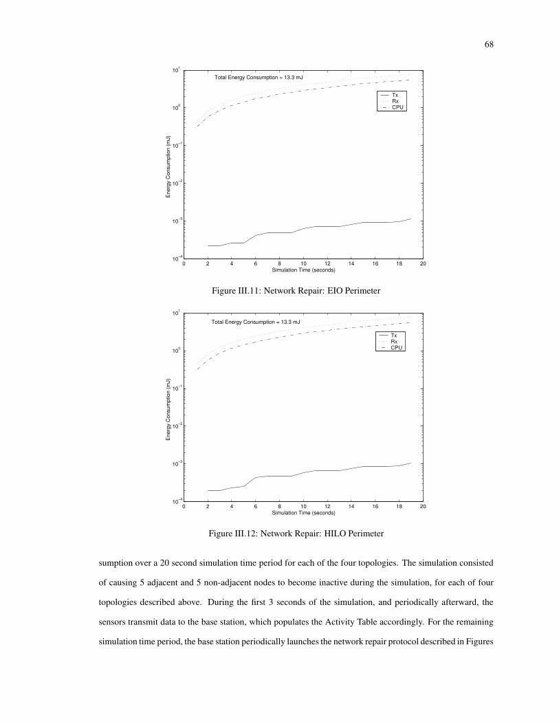
68

0 2 4 6 8 10 12 14 16 18 2010−4

10−3

10−2

10−1

100

101

Simulation Time (seconds)

Ene

rgy

Con

sum

ptio

n (m

J)

TxRxCPU

Total Energy Consumption = 13.3 mJ

Figure III.11: Network Repair: EIO Perimeter

0 2 4 6 8 10 12 14 16 18 2010−4

10−3

10−2

10−1

100

101

Simulation Time (seconds)

Ene

rgy

Con

sum

ptio

n (m

J)

TxRxCPU

Total Energy Consumption = 13.3 mJ

Figure III.12: Network Repair: HILO Perimeter

sumption over a 20 second simulation time period for each of the four topologies. The simulation consisted

of causing 5 adjacent and 5 non-adjacent nodes to become inactive during the simulation, for each of four

topologies described above. During the first 3 seconds of the simulation, and periodically afterward, the

sensors transmit data to the base station, which populates the Activity Table accordingly. For the remaining

simulation time period, the base station periodically launches the network repair protocol described in Figures

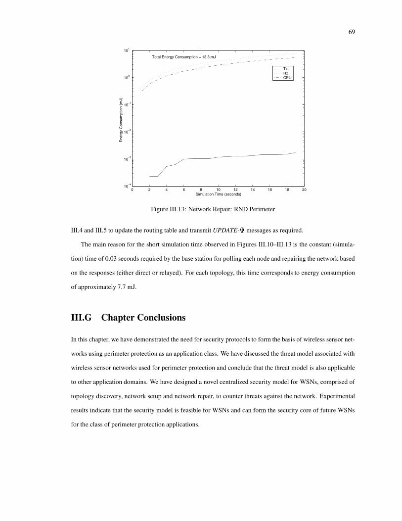
69

0 2 4 6 8 10 12 14 16 18 2010−4

10−3

10−2

10−1

100

101

Simulation Time (seconds)

Ene

rgy

Con

sum

ptio

n (m

J)

TxRxCPU

Total Energy Consumption = 13.3 mJ

Figure III.13: Network Repair: RND Perimeter

III.4 and III.5 to update the routing table and transmit UPDATE- ¤ messages as required.

The main reason for the short simulation time observed in Figures III.10–III.13 is the constant (simula-

tion) time of 0.03 seconds required by the base station for polling each node and repairing the network based

on the responses (either direct or relayed). For each topology, this time corresponds to energy consumption

of approximately 7.7 mJ.

III.G Chapter Conclusions

In this chapter, we have demonstrated the need for security protocols to form the basis of wireless sensor net-

works using perimeter protection as an application class. We have discussed the threat model associated with

wireless sensor networks used for perimeter protection and conclude that the threat model is also applicable

to other application domains. We have designed a novel centralized security model for WSNs, comprised of

topology discovery, network setup and network repair, to counter threats against the network. Experimental

results indicate that the security model is feasible for WSNs and can form the security core of future WSNs

for the class of perimeter protection applications.

Chapter IV

C-SONETS: CENTRALIZED SECURE

SELF-ORGANIZATION IN WIRELESS SENSOR

NETWORKS

We believe that P-SONETS is an efficient and secure solution for problems related to the class of perimeter

protection applications. However, it is not scalable with respect to network size. As the number of nodes

beyond a two-hop transmission range to the base station increases, the size of encrypted messages from those

nodes to the base station (and vice versa) increases. This leads to increased energy consumption by the entire

WSN, because transmission costs dominate all other costs. Further, physical failure of the single, trusted

computing base in a WSN using P-SONETS renders the network inoperable.

IV.A Introduction

In order to address the above issues in P-SONETS, we have extended the concept of employing trusted com-

puting bases to ensure secure self-organization in WSNs and designed C-SONETS. The C-SONETS protocol

suite employs multiple trusted computing bases in order to eliminate the the single-point-of-failure problem.

Further, in order to provide scalability C-SONETS ensures that the size of encrypted messages from a node

to a base station is not a function of the distance between them; rather it is a function of the number of 1-hop

neighbors discovered by that node. The novel topology discovery and key setup mechanism in C-SONETS

ensures confidentiality, authenticity, integrity, and protection from traffic analysis and replay. C-SONETS

70

71

also provides sensor nodes with the capability to establish multi-hop, pair-wise keys in order to achieve end-

to-end security between nodes, if required. New nodes can be legitimately added to an existing WSN using

C-SONETS so that they establish secure links with neighbors and can reach a trusted base station in one or

more secure hops. C-SONETS provides an efficient voting based mechanism to ensure that neighbors of a

misbehaving node can delete it from the WSN.

Pair-wise key establishment is the cornerstone of security protocols for large scale homogeneous and

heterogeneous WSNs. In C-SONETS and D-SONETS (described in Chapter V), pair-wise keys are estab-

lished after node deployment, in a deterministic manner. This is in contrast to pair-wise key pre-distribution

protocols [11, 18, 19, 37], which are probabilistic. Therefore, C-SONETS and D-SONETS trade off higher

energy consumption for better resilience, flexible network size and lower storage requirements. A significant

advantage of C-SONETS and D-SONETS compared to probabilistic approaches is that key material exposed

by a compromised node cannot be used to compromise links between uncompromised nodes, irrespective

of network size. This is because each node only possesses keys for communication with 1-hop neighbors.

All probabilistic approaches, except random pair-wise keying [11], exhibit the above vulnerability. How-

ever, even random pair-wise keying is perfectly resilient only for a fixed network size, determined at design

time, and is restricted by the amount of available on-board memory, requiring additional techniques to extend

network size.

Further, C-SONETS is agnostic of the security environment. It does not assume that nodes remain uncom-

promised until pair-wise key establishment has occurred, unlike LEAP [61]. This is because in C-SONETS,

pair-wise keys are not computed from a single master key; they are computed using keying material unique

to each sensor node and random numbers generated by base stations, resulting in better resilience to attacks

during network setup.

IV.B Background

Eschenauer and Gligor [19] discuss key pre-distribution on sensor nodes such that each pair of nodes shares

at least one key with probability . Each node possesses a key ring, formed by drawing k keys without

replacement from a set of keys S which is a random subset of a large pool of keys. After deployment, in the

key setup phase, each sensor node discovers neighbors it shares a key with.

Chan et al. [11] present three schemes for random key pre-distribution in sensor networks. The first

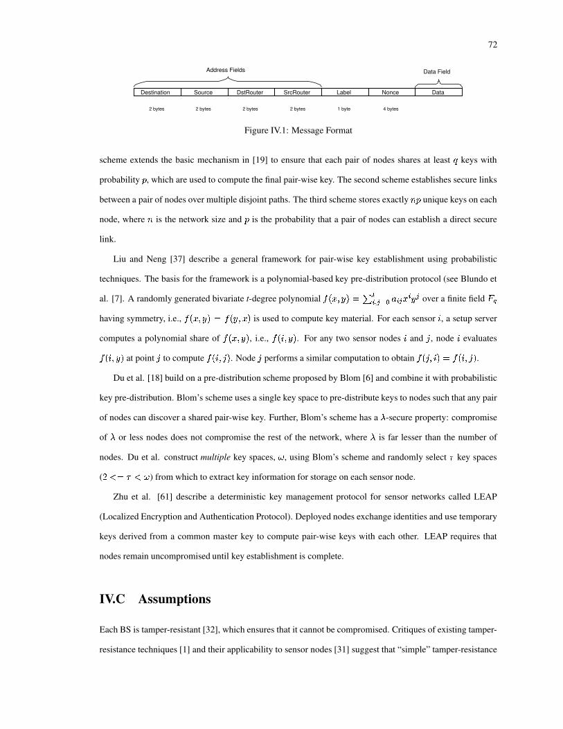
72

Data Field

Destination Source DstRouter Nonce Data SrcRouter Label

Address Fields

2 bytes 2 bytes 2 bytes 4 bytes 2 bytes 1 byte

Figure IV.1: Message Format

scheme extends the basic mechanism in [19] to ensure that each pair of nodes shares at least ¿ keys with

probability , which are used to compute the final pair-wise key. The second scheme establishes secure links

between a pair of nodes over multiple disjoint paths. The third scheme stores exactly HÀ unique keys on each

node, where H is the network size and is the probability that a pair of nodes can establish a direct secure

link.

Liu and Neng [37] describe a general framework for pair-wise key establishment using probabilistic

techniques. The basis for the framework is a polynomial-based key pre-distribution protocol (see Blundo et

al. [7]. A randomly generated bivariate t-degree polynomial k �ÂÁ ?Au � �«Ã ¹µÂÄ oGÅ;Æ6Ç µ o Á µ u o over a finite field ÈYÉhaving symmetry, i.e., k �ÂÁ ?Au � �«k � u/? Á/� is used to compute key material. For each sensor ® , a setup server

computes a polynomial share of k �ÂÁ ?Au � , i.e., k � ®D?Au � . For any two sensor nodes ® andz, node ® evaluates

k � ®D?Gu � at pointz

to compute k � ®D? zJ� . Nodez

performs a similar computation to obtain k ��z ?G® � �ck � ®�? zJ� .Du et al. [18] build on a pre-distribution scheme proposed by Blom [6] and combine it with probabilistic

key pre-distribution. Blom’s scheme uses a single key space to pre-distribute keys to nodes such that any pair

of nodes can discover a shared pair-wise key. Further, Blom’s scheme has a Ê -secure property: compromise

of Ê or less nodes does not compromise the rest of the network, where Ê is far lesser than the number of

nodes. Du et al. construct multiple key spaces, Ë , using Blom’s scheme and randomly select Ì key spaces

( �� ��Ì��Ë ) from which to extract key information for storage on each sensor node.

Zhu et al. [61] describe a deterministic key management protocol for sensor networks called LEAP

(Localized Encryption and Authentication Protocol). Deployed nodes exchange identities and use temporary

keys derived from a common master key to compute pair-wise keys with each other. LEAP requires that

nodes remain uncompromised until key establishment is complete.

IV.C Assumptions

Each BS is tamper-resistant [32], which ensures that it cannot be compromised. Critiques of existing tamper-

resistance techniques [1] and their applicability to sensor nodes [31] suggest that “simple” tamper-resistance

73

is easily broken and “complex” tamper-resistance is expensive, making it ill-suited to sensor nodes. On the

other hand, BSs must be tamper-resistant because they are gateways to the WSN and the only interface to

users of the WSN. Furthermore, the number of BSs in the WSN is limited, therefore the cost of tamper-

resistance is amortized over the life of the WSN. Each BS possesses significantly higher amount of energy,

computing power, memory and storage than sensor nodes; each BS’s radio has universal coverage in the

network. On the other hand, each sensor node has limited amounts of energy, computing power, memory and

storage, and its radio has a limited transmission range.

Each BS in the network has a unique ID and contains a list of all sensor nodes in the network. Each BS’s

ID is designed to enable all nodes in the WSN to distinguish between an ordinary node and a BS. Each BS

stores a list of unique shared keys s�Í (one per sensor node a ), a list of unique node secrets [53]Á Í (one per

sensor node a ) and a network-wide key s � , which is common to all nodes in the network. A shared key s�Íbetween a BS and node a provides a secure, out-of-band communication channel irrespective of the number

of hops between them, as we show in Section IV.E.2. Furthermore, s Í provides authentication between BS

and node a because only these two entities can successfully decrypt a message encrypted by the other using

s Í . The node secretÁ Í associated with node a is a primary component of all pair-wise keys that node a

eventually establishes with its neighbors (Section IV.D).

Each sensor node a in the network also has a unique node ID and contains s�Í , the network-wide key s � ,the unique node secret

Á Í and a one-way hash function k (e.g., the 160-bit SHA-1 hash function), which is

used for computing pair-wise keys.

Key and node secret lengths are constant at�

bits. Each BS communicates periodically with other BSs in

the network over a separate secure channel in order to exchange topology information and keying material.

The message format used by all nodes in the WSN is shown in Figure IV.1. The entire message is always

encrypted by s � and parts within are encrypted using pair-wise keys or shared keys as required. Thus, there

is no need to include a separate message digest with the original message because no part of the message

is ever transmitted in the clear, thereby ensuring that an adversary cannot tamper with specific fields of a

message without possessing at least s � . The address portion of the message is unencrypted by pair-wise

or shared keys. Encrypting the entire message, including the address portion, using s � helps prevent traffic

analysis by adversaries. If s � is leaked to an adversary, the network becomes vulnerable to traffic analysis,

but the rest of the message remains secure. Additionally, the Î%¼¶H ­ t field in the message provides freshness

and thwarts message replay attacks.

74

The adversary is assumed to be capable of compromising sensor nodes, which are not tamper-resistant.

The adversary can also launch Denial-of-Service (DoS) attacks, message replay attacks, Sinkhole and Worm-

hole and Sybil attacks [31] on the WSN.

IV.D WSN Model and Pair-wise Key Design

The WSN consists of a limited number of static or mobile BSs, each of which can support thousands of

sensor nodes. The presence of multiple, powerful BSs increases the network’s scalability during secure self-

organization, data aggregation and energy conservation. The model is applicable to a variety of domains in

which sensor nodes may be static or mobile. Each BS is a powerful entity capable of performing network

setup, query processing and energy management in the WSN. During normal operation of the WSN, the final

destination of data generated by any sensor node is one of the BSs.

A node secret is the most important component of a pair-wise key between any two nodes a and ¯ . Using

node secrets enables node-to-node authentication [11], because each node secret is unique and associated

with one and only one node in the entire WSN. Thus, a unique combination of individual node secrets would

serve as a strong pair-wise key. However, under no circumstances should a node’s secret be revealed to

another node in the WSN; otherwise the pair-wise keying mechanism will fail.

A pair-wise key between nodes a and ¯ is constructed as follows:

1. Compute ¼¶H#X¶Í+Ïl� Á Ï�Ð � and ¼¶H#X+Ï�Í(� Á Í`Ð � . The notation ¼¶H#X+Í¶Ï stands for: node v’s secret,Á Ï , obfuscated with a random number�

, and associated with node u. ¼¶H#X�Ï�Í has a similar meaning.

Random number�

is unique to the pair-wise key under construction. Symbol Ð stands for the bit-wise

XOR of the two operands.

2. Node a computes s�ͶÏ<�fk � ¼¶H#X+ͶÏbÐ Á Í � and node ¯ computes s�Ï�Í��[k � ¼¶H#X+Ï�Í�Ð Á Ï � , where k is a

one-way hash function. Observe that s�Í¶Ï = s|Ï�Í because XOR is a commutative operation.

The constraint that node secrets must not be revealed to other nodes in the WSN precludes nodes a and ¯from exchanging

Á Í andÁ Ï , respectively, in order to compute ¼¶H#XKÍ¶Ï and ¼¶H#X+Ï�Í . Thus, this step is executed

by a BS, one of a limited number of trusted entities in the WSN. This implies that nodes a and ¯ must receive

¼¶H#X+Í¶Ï and ¼¶H#X+Ï�Í , respectively, from a BS in order to execute the second step and compute pair-wise key

s|Í¶Ï (= s|Ï�Í ). Therefore, the BS employs s�Í and s|Ï to encrypt messages containing ¼¶H#X¶Í¶Ï and ¼¶H#X+Ï�Í ,respectively, and transmits those messages to nodes a and ¯ . As discussed in Section IV.C, s Í provides a

75

Message Type Function Source DestinationHELLO Neighbor discovery Node or BS Node or BS

HELLO ACK Neighbor discovery Node or BS NodeNLIST Provide list of neighbors Node BS

ONSLIST Provide list of ONSs BS NodeRTINFO Provide routing information BS Node

FWD Forward embedded message Node Node or BSSEEDATA Indicate presence of embedded message Node BS

Table IV.1: Message Types

secure, out-of-band channel for communication between a BS and node a , in addition to serving the purpose

of authentication between them.

Repeated execution of the two steps discussed above will result in each node in the WSN obtaining a

pair-wise key with each neighboring node.

An important feature of the two-step pair-wise key design is that even if the out-of-band channel between

a BS and a node were to be compromised and ONSs revealed, an adversary would still be unsuccessful in

obtaining pair-wise keys associated with that node. This is because each node must apply its own secret

(which an adversary can only obtain by physically compromising the node) to the received ONS in order to

compute the final pair-wise key with that neighbor.

IV.E Self-organization and Single-hop Pair-wise Key Establishment

(SO/SPKE)

In this section, we discuss two protocols that constitute SO/SPKE – neighbor discovery, and topology dis-

covery and key setup. During neighbor discovery, all nodes, including BSs, discover 1-hop neighbors. In

topology discovery and key setup, nodes provide local topology information to BSs and receive neighbors’

ONSs in return. Table IV.1 shows the different types of messages exchanged between nodes during execution

of SO/SPKE.

IV.E.1 Neighbor Discovery

Single-hop neighbor discovery is executed by all entities in a WSN, including sensor nodes and BSs. At some

random time after deployment, each entity broadcasts a HELLO message, encrypted with s � , to discover

76

1-hop neighbors. The message consists of the source address, the broadcast destination address, the message

label and a nonce generated by the source. Each node broadcasts a HELLO message a fixed number of times

before terminating neighbor discovery. In response to the HELLO message, each 1-hop neighbor, including

BSs, transmits a HELLO ACK message containing the original nonce present in the HELLO message. If the

nonce verifies at the original source, then that neighbor is added to the source’s neighbor list. These message

sequences are shown below (* indicates a broadcast destination):

a yÒÑd{@}b~ ^ � Ñ ?Aa6?G� }������ ?�Î%¼¶H ­ t¶Í �¯ y a {�} ~ ^ � a�?G¯&?�� }d���¡� � Ó s%?�Î%¼¶H ­ t Í �

w:x�y a {�} ~ ^ � a6? w<x ?G� }d����� � Ó sl?GÎ%¼¶H ­ t Í �H!½B®�X\U�Í�Ô±H!½B®�X´U�Í£��¯-? w:x

Nodes that discover a BS associate with it and employ it for subsequent topology discovery and pair-wise

key setup. An interesting issue that arises is that of nodes that discover multiple BSs as 1-hop neighbors and

must choose a primary BS with which to associate. For example, consider four entities, a , ¯ , BS1 and BS2,

where a and ¯ are sensor nodes, while BS1 and BS2 are base stations. Let a and ¯ be 1-hop neighbors of

both BS1 and BS2. If a chooses BS1 as its primary BS and ¯ chooses BS2, a situation arises where a obtains

an ONS to establish a pair-wise key with ¯ from BS1 (Section IV.D) and ¯ obtains an ONS from BS2. Thus,

we observe that a and ¯ may establish two pair-wise keys with each other. Nodes a and ¯ solve this problem

by choosing the key that is lexicographically greater of the two.

Subsequent to neighbor discovery, all sensor nodes initiate topology discovery and key setup (Section

IV.E.2) after receiving synchronization messages from all BSs in the WSN.

Neighbor discovery in C-SONETS is similar to that in LEAP [61], but different from that in [11, 18, 19,

37] where neighbor discovery is performed to determine all neighboring nodes ¯ with which a source node ashares a common key, polynomial or matrix elements.

IV.E.2 Topology Discovery and Key Setup

Topology discovery in C-SONETS is based on a simple invariant: For each value of a hop distance C , a BS

discovers all nodes at a distance of C hops from it before working on the topology of the WSN at a distance

77

of C<�Z) hops. Furthermore, the BS discovers WSN topology as far as C`�Z) hops and not beyond, because

security of pair-wise communications between sensor nodes is guaranteed only until that point.

Initially, C%�Q) , i.e., sensor nodes one hop away from a BS establish pair-wise keys with the help of the

BS. Let us consider the case of a sensor node a and base station BS1. First, node a transmits its neighbor list

H!½Â®�X\U�Í to BS1 in a NLIST message encrypted under both s�Í and s � as shown below:

a y�w:x ) {�}b~ ^ �Bw<x )�?Aa6? }�~VÕ'� Î ��ÖJx �b?�Î%¼¶H ­ t¶Í1?GH!½Â®�X\U�Í �A�BS1 decrypts the message and implicitly authenticates a if the inner message decrypts correctly. BS1 then

processes each node on H!½Â®�X\U Í by creating ¼¶H#X Ï�Í for each node ¯ on H!½Â®�X\U Í using the technique described

in Section IV.D and stores the ONS in the routing table entry for ¯ . As it goes through the list, BS1 may

find a node × it did not discover during neighbor discovery. Such nodes are 2-hop neighbors of BS1 and are

added to the routing table along with their hop count and node a ’s ONS, e.g., ¼¶H#X�Ø;Í . BS1 also creates ¼¶H#X+ͶÏand stores it on ¼¶H#X\½B®�X´UAÍ , i.e., the list of obfuscated node secrets of node a ’s neighbors. Subsequently, BS1

transmits ¼¶H#X\½B®�X´UAÍ to node a in an ONSLIST message, encrypting it with both s � and s|Í .¼¶H#X Ï�Í Ô Á Í Ð � ͶÏJÙ � ¼¶a&U�t+� ÇÀÚ ½�tJÛ ¯@Ü1Ô � ¼¶a-U�t+� ÇÀÚ ½BtJÛ ¯�Ü�� � a6?G¼¶H#X Ï�Í ?´��) �¼¶H#X+Ø;Í<Ô Á Í�Ð � Í¶Ø Ù � ¼¶a-U�t\� ÇJÚ ½BtJÛ ×bÜ1Ô � ¼¶a-U�t+� ÇÀÚ ½BtJÛ ×ÝÜ@� � a�?�¼¶H#X\Ø;Í&?�� �¼¶H#X+Í+Ï�Ô Á ÏÝÐ � Í+Ï Ù ¼¶H#X\½B®�X´U�Í:Ô�¼¶H#X+½Â®�X\U�Í>�[�¯-?G¼¶H#X+ͶÏ�2�?�Þ-¯�¨�H!½Â®�X\U�Íw<x ) y a {�}b~ ^ � a�? w<x )@? }b~�Õ&� � Î xY��ÖJx �b?�Î%¼¶H ­ t prqJß ?�¼¶H#X+½Â®�X\U�Í �A�

Upon receipt and decryption of the ONSLIST message from BS1, node a proceeds to compute the pair-

wise key with each neighbor as discussed in Section IV.D.

BS1 also transmits a RTINFO message to each node ¯ on H!½Â®�X\UGÍ containing ¼¶H#X+Ï�Í and routing informa-

tion. The routing information consists of a neighbor ID (e.g., a ) and the number of hops � in which node ¯can reach BS1 via a (e.g., 2). If both a and ¯ are 1-hop neighbors of BS1, then � is set to -1 in the RTINFO

message indicating that neither node requires a router to reach the BS.

=¶U�®°H#k/¼KÏ£Ô � a6?G¼¶H#X+Ï�Í-?´��) �

78

w<x ) y ¯ {�}b~ ^ � ¯&? w<x )@? }b~VàJ��� � Ö Î%È � ?�Î%¼¶H ­ t prqJß ?A=¶U�®°H#k/¼KÏ �A� ?�Þ-¯|¨�H!½Â®�X\U�Í1?GH!½Â®�X\U p6qÀß=+U�®°H#k/¼KØ�Ô � a6?G¼¶H#X+Ø;Í1?�� �

w:x ) y × {�}b~ ^ � ×d? w<x )@? }b~Vá��B� � Ö Î%È � ?GÎl¼¶H ­ t p6qÀß ?G=+U�®°H#k/¼KØ � ?�Þ-×â¨�H!½Â®�X\U�Í1?A×äã¨�H!½Â®�X\U prqJßUpon receipt and decryption of the RTINFO message from BS1, each node ¯ computes its pair-wise key

with node a and stores the routing information, if any, that enables ¯ to reach BS1 via a . We observe that

nodes unable to discover any BS during neighbor discovery do so via RTINFO messages. Using information

from these messages, these nodes choose a primary BS and associate with it.

After the primary BS is chosen, a neighbor that is closer to that BS is designated as the primary router.

For example, node × could designate node a as its primary router after receiving the RTINFO message shown

above.

At this point, all BSs have discovered nodes that are two hops away and distributed ONSs to them. They

discover nodes beyond two hops as follows. Consider a 2-hop node × that has a route to base station BS1

via node a with which it has established a pair-wise key s Ø;Í . Node × may also have established pair-wise

keys with other neighbors that are two hops away from a BS, but not with those that are three hops away.

Thus, it creates a neighbor list H!½B®�X\UGØ , consisting of these neighbors’ IDs, places it in an NLIST message

and encrypts the message using s�Ø . It then embeds the NLIST message in a FWD (i.e., forward) message,

encrypting both with with s�Ø;Í . Finally, it sets BS1 as the destination and node a as the ��X\U � ¼¶a&U�t+= (see

Figure IV.1).

× y�w<x ) {�}b~ ^ ��w<x )@?A×d?Ga�? }b~Vá>Õ&� Èdåâ��?GÎ%¼¶H ­ t+Ø�? }�~VáV� Î ��ÖJx �b?AH!½B®�X´U�Ø �A�G�The FWD message is node × ’s request to node a to forward the NLIST message to BS1. The fact that

the ��X\U � ¼¶a&U�t+= field of the message contains its address ensures that node a processes the message further

instead of throwing it away based on the ��X\U field. Node a decrypts the inner part of the message using s Ø;Íand verifies the nonce for recency to ensure that the message has not been replayed. Node a then re-labels the

FWD message as a SEEDATA message, replaces the nonce with its own and transmits the message to BS1.

a y�w:x ) {�} ~ ^ ��w<x )@?A×d?Ga�? } ~ Õ-��xY}�} � � � � ?GÎl¼¶H ­ t Í ? } ~ áV� Î ��ÖJx �b?AH!½B®�X´U Ø �A�G�

79

Upon receipt and verification of the SEEDATA message, BS1 extracts its payload and decrypts it using

s|Ø to obtain the embedded NLIST message. At this point, the situation is exactly the same as that when node

a transmitted its NLIST message to BS1 directly. Thus, BS1 takes the same actions as before and transmits

an ONSLIST message to node × and RTINFO messages to all nodes in the incoming NLIST message that

are new. BS1 has thus discovered nodes three hops away from it.

w<x ) y × {@}b~ ^ � ×�? w<x )�? }�~Vá�� � Î xY��ÖJx �b?�Î%¼¶H ­ t prqJß ?�¼¶H#X+½Â®�X\U�Ø �G� ?�Þ/u|¨�H!½Â®�X\U�Ø=¶U�®°H#k/¼ � Ô � ×d?�¼¶H#X+Ø � ?G� � ?�Þ-u�¨�H!½B®�X\U�Ø

w<x ) y u {�} ~ ^ � u/? w:x )�? } ~Væ �B� � Ö Î%È � ?GÎl¼¶H ­ t¶p6qÀß+?G=+U�®°H#k/¼ � �G� ?�Þ/u|¨�H!½Â®�X\U ØThe procedure discussed above is executed repeatedly until all nodes in the network have been discovered

by at least one BS and have established pair-wise keys with all their 1-hop neighbors. Since the network size

is finite as is the distance between the farthest node connected to the network and a BS, the protocol eventually

terminates. Thus, we accomplish secure self-organization of a WSN and enable nodes to operate securely in

a pair-wise manner.

The topology discovery and key setup protocol discussed in this section is unique; none of the existing

probabilistic or deterministic protocols perform topology discovery simultaneously with key setup as dis-

cussed above.

IV.F Performance Analysis

All protocols described in this chapter were simulated using SENSE (Sensor Network Simulator and Emula-

tor) [12], an event-driven simulator capable of simulating sensor networks of up to 5000 nodes. Table IV.2

shows initial values of configuration parameters used in our simulations. These parameters are common to

all protocols described in this paper. For all simulations, node co-ordinates were randomly generated and

assigned by the simulator producing a random WSN topology. Message hashing is performed using SHA-1,

which consumes approximately 0.65 � J/byte (see Potlapally et al. [49]). Message encryption and decryption

algorithm is performed using RC5 in electronic code book (ECB) mode. We use SHA-1 as the one-way hash

function to compute pair-wise keys.

We are aware that the ECB mode of RC5 has many vulnerabilities that prevent it from being used in a

80

Parameter ValueField size 500m x 500m

Node transmission range 75 mBS transmission range universal coverage

Total number of nodes in WSN 100 to 1000Initial node energy 1e8 J

Tx energy consumed/node 83*t*k mJ, t=bit time, k=#bitsRx energy consumed/node 33*t*k mJ, t=bit time, k=#bitsIdle energy consumed/node 3.3*t mJ, t=time

RC5 key setup energy consumption 66.54 � JRC5 encrypt/decrypt energy consumption 0.76 � J/byte

SHA-1 energy consumption 0.65 � J/byteRatio of BSs to total number of nodes in WSN 0.01

Maximum number of attempts for neighbor discovery per node 10

Table IV.2: WSN Configuration Parameters

real-world, practical system and do not advocate its use in a wireless sensor network either. We employ it

only to evaluate the security protocols in terms of energy consumption. Potlapally et al. have empirically

measured the energy consumed by RC5 in ECB mode to encrypt and decrypt one byte of data. We use this

information directly to empirically determine the overall energy consumed by the protocols to accomplish

secure self-organization. The proposed protocols will work correctly with RC5 or AES-128 in Integrity

Aware Parallelizable Mode (IAPM) [29], OCB [50], eXtended CBC (XCBC) and other similar modes.

SO/SPKE is evaluated using four metrics: energy consumption, pair-wise key setup time, node to BS hop

count and node degree. Network sizes range from 100 to 1000 nodes.

IV.F.1 Energy consumption

Figure IV.2 shows the mean total energy consumed per node, including communication and security. Energy

consumed for communication is the dominant component of the total energy consumption. Energy consump-

tion ranges from 0.65 J/node to 22 J/node. As expected, energy consumption increases with network size due

to higher cost of neighbor discovery and topology discovery (transmitting larger NLIST messages and, re-

ceiving larger NLIST, ONSLIST and RTINFO messages). Figure IV.2 also shows that the increase in energy

consumption is approximately O( H�ç ), where H is the network size.

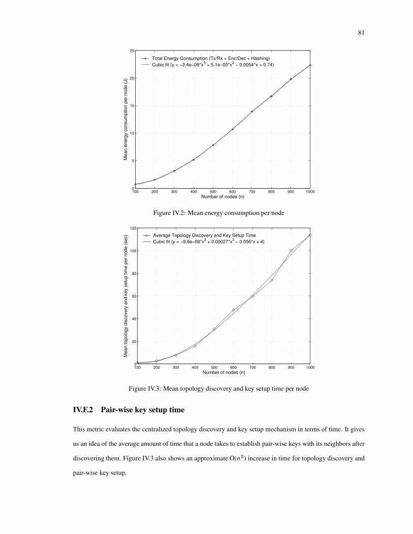
81

100 200 300 400 500 600 700 800 900 10000

5

10

15

20

25

Number of nodes (n)

Mea

n en

ergy

con

sum

ptio

n pe

r nod

e (J

)

Total Energy Consumption (Tx/Rx + Enc/Dec + Hashing)Cubic fit (y = −2.4e−08*x3 + 5.1e−05*x2 − 0.0054*x + 0.74)

Figure IV.2: Mean energy consumption per node

100 200 300 400 500 600 700 800 900 10000

20

40

60

80

100

120

Number of nodes (n)

Mea

n to

polo

gy d

isco

very

and

key

set

up ti

me

per n

ode

(sec

) Average Topology Discovery and Key Setup TimeCubic fit (y = −9.8e−08*x3 + 0.00027*x2 − 0.056*x + 4)

Figure IV.3: Mean topology discovery and key setup time per node

IV.F.2 Pair-wise key setup time

This metric evaluates the centralized topology discovery and key setup mechanism in terms of time. It gives

us an idea of the average amount of time that a node takes to establish pair-wise keys with its neighbors after

discovering them. Figure IV.3 also shows an approximate O( H6ç ) increase in time for topology discovery and

pair-wise key setup.

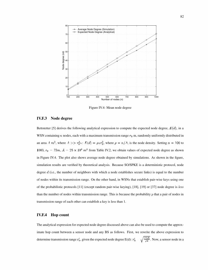
82

100 200 300 400 500 600 700 800 900 10000

10

20

30

40

50

60

70

80

Number of nodes (n)

Nod

e de

gree

(nd)

Average Node Degree (Simulation)Expected Node Degree (Analytical)

Figure IV.4: Mean node degree

IV.F.3 Node degree

Bettstetter [5] derives the following analytical expression to compute the expected node degree,}|� I � , in a

WSN containing H nodes, each with a maximum transmission range = Æ m, randomly uniformly distributed in

an area� E�¾ , where

� 2�2è=K¾ÆKé :}|� I � �fê é =K¾Æ , where ê%�fH�ã � , is the node density. Setting H��T)\*�* to

)\*@*�* , = Æ �ëm�S�E ,� �ë�@S�ì�)+*�íbE�¾ from Table IV.2, we obtain values of expected node degree as shown

in Figure IV.4. The plot also shows average node degree obtained by simulations. As shown in the figure,

simulation results are verified by theoretical analysis. Because SO/SPKE is a deterministic protocol, node

degree I (i.e., the number of neighbors with which a node establishes secure links) is equal to the number

of nodes within its transmission range. On the other hand, in WSNs that establish pair-wise keys using one

of the probabilistic protocols [11] (except random pair-wise keying), [18], [19] or [37] node degree is less

than the number of nodes within transmission range. This is because the probability that a pair of nodes in

transmission range of each other can establish a key is less than 1.

IV.F.4 Hop count

The analytical expression for expected node degree discussed above can also be used to compute the approx-

imate hop count between a sensor node and any BS as follows. First, we rewrite the above expression to

determine transmission range =�îÆ , given the expected node degree E(d): =�îÆ �fï Yð �DñòDó . Now, a sensor node in a

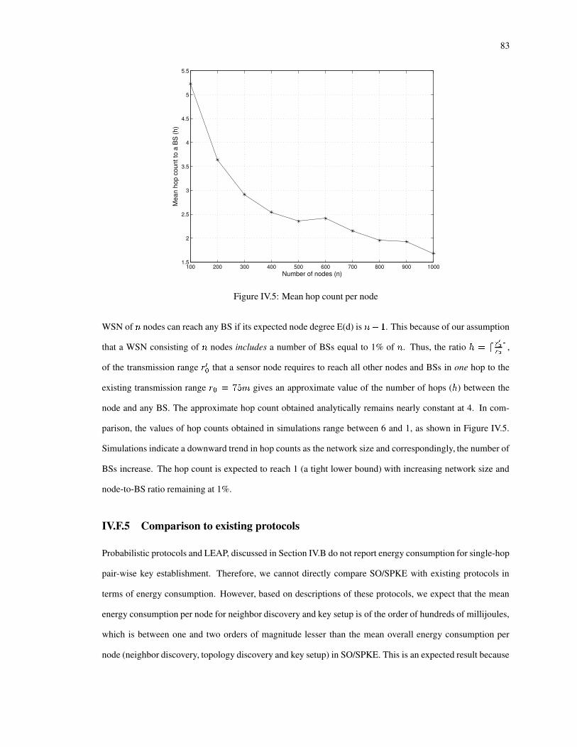
83

100 200 300 400 500 600 700 800 900 10001.5

2

2.5

3

3.5

4

4.5

5

5.5

Number of nodes (n)

Mea

n ho

p co

unt t

o a

BS

(h)

Figure IV.5: Mean hop count per node

WSN of H nodes can reach any BS if its expected node degree E(d) is H���) . This because of our assumption

that a WSN consisting of H nodes includes a number of BSs equal to 1% of H . Thus, the ratio C��Òô ³Gõö³ öK÷ ,of the transmission range =�îÆ that a sensor node requires to reach all other nodes and BSs in one hop to the

existing transmission range =\��Tm�SKE gives an approximate value of the number of hops ( C ) between the

node and any BS. The approximate hop count obtained analytically remains nearly constant at 4. In com-

parison, the values of hop counts obtained in simulations range between 6 and 1, as shown in Figure IV.5.

Simulations indicate a downward trend in hop counts as the network size and correspondingly, the number of

BSs increase. The hop count is expected to reach 1 (a tight lower bound) with increasing network size and

node-to-BS ratio remaining at 1%.

IV.F.5 Comparison to existing protocols

Probabilistic protocols and LEAP, discussed in Section IV.B do not report energy consumption for single-hop

pair-wise key establishment. Therefore, we cannot directly compare SO/SPKE with existing protocols in

terms of energy consumption. However, based on descriptions of these protocols, we expect that the mean

energy consumption per node for neighbor discovery and key setup is of the order of hundreds of millijoules,

which is between one and two orders of magnitude lesser than the mean overall energy consumption per

node (neighbor discovery, topology discovery and key setup) in SO/SPKE. This is an expected result because

84

existing protocols require each node to only broadcast either its identity (LEAP and random pair-wise keying)

or its key ring, which other nodes in the vicinity receive and employ in order to compute pair-wise keys. On

the other hand, SO/SPKE requires nodes to first discover all neighbors using a combination of broadcast and

unicast messages, following which NLIST messages are repeatedly unicast until they reach a BS. However,

we show below that while existing probabilistic protocols consume less energy, they require more storage,

have lower resilience (except random pair-wise keying) and have lower node degrees, thereby reducing the

number of redundant paths to other nodes in the network.

For ease of discussion, we label the basic probabilistic protocol in [19] as P1, ¿ -composite and random

pair-wise keying protocols in [11] as P2, the polynomial-based protocol in [37] as P3 and the matrix-based

protocol in [18] as P4.

In SO/SPKE, similar to LEAP, each node stores exactly I pair-wise keys, where I is the number of

neighbors it discovers, i.e., its node degree. Therefore, each node in a 1000-node WSN stores 65 keys, as

shown in Figure IV.4. In P1, P2 and P4 the number of keys stored is a function of a global connectivity

parameter�rø

, the desired probability with which a pair of nodes can establish a secure link and the network

size H . Thus, in P1 and P2, each node stores approximately 200 keys for Hâ�¢)\*�*@* , ��ø �h*1R ù�ù@ù�ù@ù and

«�Ò*1R g . Correspondingly, each node in P4 stores 200*( Ê +1) keys spaces, where ½ Ç E Ú I Ç is a security

parameter [18]. In P3, each node stores X î � U6�Z) � keys, where X î is the number of polynomial shares stored

on the node and U is the degree of the polynomial. An important feature of P1, P2, P3 and P4 is that they

are based on random graph theory which provides a framework to compute the number of keys required to

support networks of different sizes. Thus, by storing 200 keys, these protocols can support a network of up to

10,000 nodes. In SO/SPKE, each node would store approximately 700 keys for a 10,000-node WSN. Because

the number of BSs increases with increase in network size and hop counts tend toward 1, we can restrict the

node degree in SO/SPKE to a fixed value I , thereby ensuring that nodes store no more than I keys, while

retaining the property that each node is able to reach a BS.

In P1, P2, P3 and P4 node degree is a function of the desired probability with which each pair of nodes

can establish a secure link. Specifically, I��ú Ñ`� H��è) � in P1, the ¿ -composite protocol in P2, P3 and

P4; I�� § � õ� in the random pair-wise keying protocol in P2, where E is the number of keys and Hrî is the

expected number of nodes in transmission range. Eschenauer and Gligor show in [19] that for Hè�û)+*�*�*and

�rø �ë*'R ù@ù�ù@ù�ù , node degree Il�ü)+ù approximately. Similarly, for H��ü)+*�*@* , Eý�ë��*�* and H6î��ëþ>S ,node degree I<�W)+g approximately in random pair-wise keying protocol from P2. In contrast, node degree in

85

SO/SPKE and LEAP is equal to the expected number of nodes in transmission range of a node, i.e., its 1-hop

neighbors.

IV.G Multi-hop Pair-Wise Key Establishment (MPKE)

During WSN operation, a sensor node may need to establish a pair-wise key with another node that is multiple

hops away from it. In C-SONETS, MPKE is an extension of SPKE. Consider two arbitrary nodes a and ¯that are 2 or more hops away from each other. If a wants to establish a pair-wise key with ¯ , it transmits an

ONSREQ message containing ¯ ’s ID, either in a single hop or via multiple hops depending upon its distance

from its BS. In response, the BS transmits to a and ¯ , ONSREPLY messages containing tuples P¯-?G¼¶H#X Ï�Í jand PÂa6?G¼¶H#X Í¶Ï j , respectively. Nodes a and ¯ can then compute the pair-wise key.

We simulated MPKE for a 100-node WSN in which the source node a is 1, 7 and 14 hops away from

the BS and verified the correctness of our protocol. The verification consisted of ensuring that both a and ¯computed the same pair-wise key s�Í¶Ï and s|Ï�Í , respectively. The energy consumption of nodes participating

in this protocol is similar to that of SPKE. The distance of the source node from its primary BS is the

most important factor governing energy consumption in MPKE. Energy consumption for this protocol is

indirectly related to the number of nodes in the WSN because the latter, in conjunction with the number of

BSs, determine the average distance between a node and a BS.

IV.H Node Addition

Node addition is typically employed to augment an existing WSN and ensure that the network remains con-

nected. Each BS receives the node ID, shared key and node secret of each new node being deployed via an

out-of-band secure channel from the network controller, e.g., an unmanned aerial vehicle (UAV) flying over

a WSN deployed in a hostile area. After deployment, each new node executes SO/SPKE with two minor

changes to the neighbor discovery protocol. The first is that new nodes broadcast NEW HELLO messages

instead of HELLO messages. This enables existing nodes to determine that a new node is attempting to join

the WSN. The second change is that the HELLO ACK message from an existing node a to a new node ¯includes the ID of a ’s primary BS and its distance to that BS. After node ¯ completes neighbor discovery, it

chooses a primary BS and router based on the minimum distance to a BS, breaking ties arbitrarily. Node ¯then proceeds to execute pair-wise key setup discussed in Section IV.E.2.

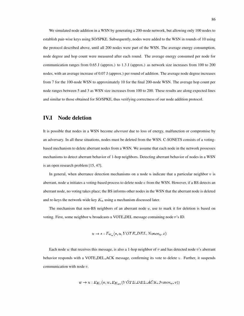
86

We simulated node addition in a WSN by generating a 200-node network, but allowing only 100 nodes to

establish pair-wise keys using SO/SPKE. Subsequently, nodes were added to the WSN in rounds of 10 using

the protocol described above, until all 200 nodes were part of the WSN. The average energy consumption,

node degree and hop count were measured after each round. The average energy consumed per node for

communication ranges from 0.65 J (approx.) to 1.3 J (approx.) as network size increases from 100 to 200

nodes, with an average increase of 0.07 J (approx.) per round of addition. The average node degree increases

from 7 for the 100-node WSN to approximately 10 for the final 200-node WSN. The average hop count per

node ranges between 5 and 3 as WSN size increases from 100 to 200. These results are along expected lines

and similar to those obtained for SO/SPKE, thus verifying correctness of our node addition protocol.

IV.I Node deletion

It is possible that nodes in a WSN become aberrant due to loss of energy, malfunction or compromise by

an adversary. In all these situations, nodes must be deleted from the WSN. C-SONETS consists of a voting-

based mechanism to delete aberrant nodes from a WSN. We assume that each node in the network possesses

mechanisms to detect aberrant behavior of 1-hop neighbors. Detecting aberrant behavior of nodes in a WSN

is an open research problem [15, 47].

In general, when aberrance detection mechanisms on a node a indicate that a particular neighbor ¯ is

aberrant, node a initiates a voting-based process to delete node ¯ from the WSN. However, if a BS detects an

aberrant node, no voting takes place; the BS informs other nodes in the WSN that the aberrant node is deleted

and re-keys the network-wide key s � using a mechanism discussed later.

The mechanism that non-BS neighbors of an aberrant node ¯ , use to mark it for deletion is based on

voting. First, some neighbor a broadcasts a VOTE DEL message containing node ¯ ’s ID.

a yÿÑ�{>}b~ ^ � Ñ ?Aa6?�� � � } � }d� ?�Î%¼¶H ­ t¶Í1?G¯ �Each node × that receives this message, is also a 1-hop neighbor of ¯ and has detected node ¯ ’s aberrant

behavior responds with a VOTE DEL ACK message, confirming its vote to delete ¯ . Further, it suspends

communication with node ¯ .× y a {�} ~ ^ � a�?G×d? } ~ á@Õ-� � � � } � }d� � Ó sl?GÎ%¼¶H ­ t Ø ?A¯ �A�

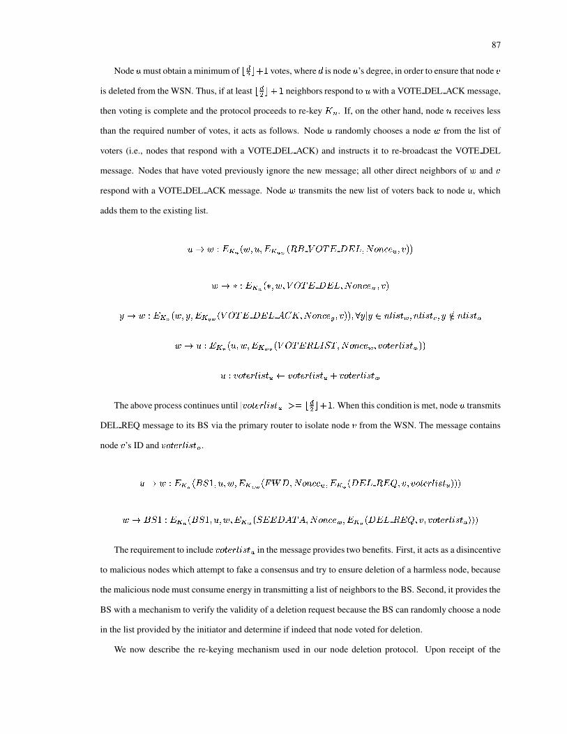
87

Node a must obtain a minimum of ��¾ � ��) votes, where I is node a ’s degree, in order to ensure that node ¯

is deleted from the WSN. Thus, if at least ��¾ � ��) neighbors respond to a with a VOTE DEL ACK message,

then voting is complete and the protocol proceeds to re-key s � . If, on the other hand, node a receives less

than the required number of votes, it acts as follows. Node a randomly chooses a node × from the list of

voters (i.e., nodes that respond with a VOTE DEL ACK) and instructs it to re-broadcast the VOTE DEL

message. Nodes that have voted previously ignore the new message; all other direct neighbors of × and ¯respond with a VOTE DEL ACK message. Node × transmits the new list of voters back to node a , which

adds them to the existing list.

a y × {@} ~ ^ � ×�?Aa6? } ~ Õ�á��B��w � � � } � }d� ?GÎ%¼¶H ­ t Í ?A¯ �A�× yÿÑ�{�} ~ ^ � Ñ ?A×d?�� � � } � }d� ?�Î%¼¶H ­ t Ø ?G¯ �

u y × {�}b~ ^ � ×d?Gu-? }b~ æ á¡� � � � } � }�� � Ó sl?GÎ%¼¶H ­ t � ?G¯ �G� ?�Þ/u!L u|¨�H!½B®�X\U�Ø�?AH!½Â®�X\U�Ï@?AuFã¨�H!½Â®�X\U�Í× y a {�}b~ ^ � a�?G×d? }�~Vá@Õ-� � � � }d����Ö>x ��?GÎ%¼¶H ­ t¶ØY?G¯>¼¶U�t+=K½Â®�X\U�Ø �A�

a { ¯>¼¶U�t+=K½Â®�X\U�Í<Ô±¯J¼¶U�t+=K½Â®�X\U�Í£�(¯>¼¶U�t+=K½Â®�X\U�ØThe above process continues until L ¯J¼¶U�t+=¶½B®�X´U Í LJ2 ���

�¾ � ��) . When this condition is met, node a transmits

DEL REQ message to its BS via the primary router to isolate node ¯ from the WSN. The message contains

node ¯ ’s ID and ¯J¼¶U�t+=¶½B®�X´U Í .a y × {>} ~ ^ �Bw:x )�?Ga�?G×d? } ~ Õ�áV� Èdåâ��?�Î%¼¶H ­ t Í ? } ~ Õ/� � }d� ��}�� ?A¯-?A¯J¼¶U�t\=K½B®�X\U Í �A�A�

× y�w:x ) {@} ~ ^ ��w<x )@?Aa6?A×d? } ~ áV� xY}d} � � � � ?�Î%¼¶H ­ t Ø ? } ~ Õ/� � }d� ��}�� ?G¯&?G¯>¼¶U�t+=K½Â®�X\U Í �A�A�The requirement to include ¯>¼¶U�t+=K½Â®�X\UAÍ in the message provides two benefits. First, it acts as a disincentive

to malicious nodes which attempt to fake a consensus and try to ensure deletion of a harmless node, because

the malicious node must consume energy in transmitting a list of neighbors to the BS. Second, it provides the

BS with a mechanism to verify the validity of a deletion request because the BS can randomly choose a node

in the list provided by the initiator and determine if indeed that node voted for deletion.

We now describe the re-keying mechanism used in our node deletion protocol. Upon receipt of the

88

DEL REQ message from node a , a designated BS generates and distributes a new s � . An important require-

ment of the re-keying mechanism in a multiple-BS WSN is that only one BS be allowed to perform re-keying,

to ensure that all nodes obtain the same s � . This requirement can be met using simple offline mechanisms

such as choosing the BS with least (or greatest) ID or online mechanisms such as a rotation scheme in which

the BS to perform this task is periodically changed according to some order, e.g., increasing or decreasing

order of BS IDs.

The designated BS transmits the new key to each node a NEWKEY message that also contains node

¯ ’s ID. Thus, all nodes that established either single-hop or multi-hop pair-wise keys with node ¯ delete

those keys from memory and delete node ¯ from their neighbor lists. If some node u chose ¯ as its primary

router during topology discovery, then u must now choose a new router from its table containing routing

information. In a pathological case, if all routers between a node and a BS are deleted from the WSN, then

that node is isolated from the WSN. As shown in Figure IV.4, the average node degree of a 1000-node WSN

is approximately 65. Therefore, assuming a random distribution of the WSN, approximately 65 nodes must

be deleted to isolate each node.

w:x ) y a {�} ~ ^ � a6? w:x )�? } ~ Õ'� Î } åâs }d� ?�Î%¼¶H ­ t¶prqJ߶?Gs î� ?G¯ �G� ?�Þ/a�¨�å x Î�L a�¬��¯BS1 continues to use the old network-wide key s � to encrypt NEWKEY messages until all nodes obtain

the new key. This is not a problem because important parts of the message are encrypted by the shared key

between BS1 and each node a .

Node deletion or revocation in C-SONETS relies primarily on voting, a technique suggested in [11].

Pair-wise keys shared between the deleted node and its neighbors are removed from their storage in a manner

similar to that described in [19]. In C-SONETS the network-wide key must be re-keyed after node deletion.

In all four probabilistic protocols discussed previously, a mechanism to ensure that all keys present on the

deleted node are removed from other nodes in the network, is required.

We simulated the node deletion protocol in a manner similar to the simulation of MPKE. In this case,

source node a ’s node degree and distance to a BS are important factors in determining energy consumption

of the WSN. Additionally, all nodes must expend energy in receiving and decrypting the NEWKEY message

containing the new value of s � and the ID of the deleted node. We simulated node deletion in a 100-node

WSN with the source at distances greater than 1 hop to verify its correctness. The verification consisted of

89

ensuring that all references to the deleted node were removed from the WSN and that nodes which used it as

a router chose a new router to their primary BS.

IV.J Security Analysis

We evaluate C-SONETS in terms of network and data security. Both network and data security are affected

if sensor nodes are compromised. We analyze the extent of the effect of node compromise on network and

data security in our approach.

IV.J.1 Effects of node compromise

Each sensor node a is pre-loaded with s � , s|Í andÁ Í (Section IV.C). Now, assume the worst-case sce-

nario: node a is compromised immediately after deployment, i.e., even before neighbor discovery. Thus, the

adversary has access to the two keys and the node secret.

Neighbor discovery uses s � to encrypt all parts of the HELLO and HELLO ACK messages. Therefore,

the adversary can launch spoofing and message replay attacks against neighbor discovery using a compro-

mised node. Spoofing cannot be prevented during neighbor discovery if the attack is launched from a com-

promised node; however, it is limited to the 1-hop neighborhood of the compromised node. The adversary can

also launch message replay attacks during neighbor discovery, but the presence of a Î%¼¶H ­ t in the message

ensures that non-compromised sensor nodes can determine that a particular message is being replayed.

Let us assume that node compromise is not detected by the end of the neighbor discovery process. Using

compromised node a , the adversary can subsequently disrupt topology discovery, which depends on the

forwarding mechanism on each sensor node, by launching a selective forwarding attack. Let a neighbor ¯of node a learn that a is on one of the paths to its BS. Thus, ¯ requests a to forward its NLIST message

to the BS, but node a simply drops it. However, in order to ensure that it is not detected, node a forwards

some messages from other nodes. Our topology discovery protocol thwarts the selective forwarding attack

by ensuring that ¯ can find all alternate routes to its BS that do not go through a . On the other hand, node

a itself may have to depend on neighbors to forward its NLIST message to a BS. Assume that the message

successfully reaches the BS. Now, the question is: Does the message contain a valid neighbor list or garbage?

If it contains a valid list, then the adversary can remain undetected, otherwise the BS will determine that node

a is aberrant and simply not transmit to it either routing information or ONSs.

90

If node a ’s compromise remains undetected until pair-wise key setup is complete, then data security in

node a ’s 1-hop neighborhood is affected. The adversary can modify or delete data and drop data packets

transmitted to it by neighbors. Thus, the affect on data security is highly localized.

Additionally, node a can disrupt, but not prevent, MPKE by dropping some or all ONSREQ messages

that it receives. The adversary can launch spoofing and selective forwarding attacks against node addition.

In response to a HELLO message from a new node × , node a can announce itself as a BS and proceed to

provide × with spurious routing information and keys. However, other non-compromised nodes provide node

× with their hop counts to the nearest BS. If none of the counts is 1, then node × can determine that node

a ’s announcement is false. However, pathological situations in which node a is the only node one hop away

from the BS could cause × to believe a . Finally, the adversary can initiate node deletion by falsely accusing

a neighbor of aberrant behavior. However, the voting requirement will defeat the adversary’s attempt because

none of the neighbors will vote in the affirmative. Furthermore, a BS’s ability to verify consensus among

nodes regarding node deletion ensures that the adversary cannot illegally delete a node.

An important conclusion we can draw from the above discussion is that node compromise has a localized

effect and more importantly, that compromise of a single node does not lead to compromise of uncompro-

mised nodes or links (due to the pair-wise key design discussed in Section IV.D).

Node collusion, in which compromised nodes collude in order to compromise other nodes and links in

the WSN, may affect C-SONETS. While we have not studied its effects in detail, we observe the following.

The number of disjoint neighborhoods formed in an H -node WSN with node degree}|� I � is approximately

�� Vð �Dñ � . Therefore, to compromise a WSN established using C-SONETS via node collusion two conditions

must be satisfied: (i) at least one node from each neighborhood is compromised and (ii) each compromised

node must be able to expose its pair-wise keys to colluders from other neighborhoods.

Comparison to existing protocols

Random pair-wise keying [11] has the same property as C-SONETS that node compromise causes compro-

mise of only those links associated with the compromised node. This is because in random pair-wise keying,

each pre-distributed pair-wise key is unique to a pair of nodes a and ¯ : none of the other nodes in the network

possess this key. If, after deployment, nodes a and ¯ are in transmission range of each other, then they com-

municate securely using their common key. Otherwise, they cannot communicate with each other. Thus, if a

node is compromised, the only links compromised are those associated with this node. The basic probabilistic

91

protocol [19], ¿ -composite scheme [11], polynomial-based scheme [37] and matrix-based scheme [18] are

vulnerable to node compromise that leads to compromise of links between uncompromised nodes. Liu and

Neng show in [37] that a WSN in which probability of local connectivity is 0.33 and each node stores 200

keys, is completely compromised when approximately 550 nodes are compromised. As discussed in Section

IV.F, in the probabilistic schemes, 200 keys can support networks of up to 10,000 nodes.

IV.J.2 Resilience to known attacks

The known attacks we consider are Sinkhole, Sybil, Wormhole and HELLO flooding [31] and node replica-

tion. We show that our approach is resilient to these attacks and can even avoid some of them. We assume

that the adversary can launch these attacks when it believes they are most effective, that it can compromise

or add malicious nodes to the WSN and that it possesses at least s � , the network-wide key.

Sinkhole attack

In this attack, the adversary advertises that it is in the vicinity of a BS, thereby causing diversion of all traffic

toward itself, i.e., the Sinkhole. In our approach, sensor nodes do not advertise routes to neighbors; only BSs

do and each BS directly communicates with the destination node securely, to provide routing information.

Each BS computes routes from a certain node to itself, based on information received from all nodes that

communicate with it.

Sybil attack

In a Sybil attack, a single node presents multiple identities to other nodes in the network. Our approach

thwarts malicious nodes from obtaining either key material or topological information because each node amust implicitly authenticate itself to a BS using an ID-based key s�Í . Thus, even if it succeeds in presenting

different identities to nodes in its vicinity, the node ultimately fails to obtain useful information because of

its inability to decrypt messages from a BS that contain key material and routing information.

Wormhole attack

Wormhole attacks succeed when two distant colluding nodes understate the distance between them and attract

traffic toward themselves. As stated earlier, no sensor node in our approach advertises routes or distances. A

92

node can only inform a BS about its immediate neighbors. If BSs collude, then this attack succeeds against

our approach; however, the foundation of C-SONETS is that BSs cannot be compromised (Section IV.C).

HELLO flood attack

In this attack, a distant laptop-class adversary announces itself as a 1-hop neighbor to most or all nodes in the

network. This attack is easily detected and thwarted during the topology discovery and key setup protocol.

When a BS notices that all its neighbors, irrespective of distance, indicate that the adversary is one hop away

from them, it simply refuses to assign any keying material for nodes to communicate with the adversary.

Node replication

In this attack, the adversary replicates sensor nodes and distributes replicas throughout the WSN. This attack

can be thwarted by C-SONETS in one of two ways. The first is to restrict each node’s degree at design time

by preventing a node from discovering more than I neighbors. Thus, even if an adversary replicates nodes,

they will be unable to join the WSN. However, this restriction affects future attempts to add legitimate nodes

to the WSN. A possible solution is to let BSs broadcast a node degree increase message to all nodes. The

second method to thwart node replication is to let BSs exchange topology information periodically. Thus, if

BSs find the same node in different routing tables but with different neighbors, then they can determine that

it has been replicated and delete all instances of the node.

IV.K Chapter Conclusions

In this chapter, we have demonstrated an efficient and scalable centralized mechanism to ensure that sensor

nodes deployed in an area of interest self-organize securely, resulting in a resilient WSN. We have shown that

key management in C-SONETS, while expensive compared probabilistic approaches, is cost-effective for

heterogeneous WSNs. We have also demonstrated that C-SONETS is more resilient to attacks and flexible

compared to probabilistic approaches.

Chapter V

D-SONETS: DISTRIBUTED SECURE

SELF-ORGANIZATION IN WIRELESS SENSOR

NETWORKS

V.A Introduction

In this chapter we discuss D-SONETS, which is the third protocol suite in SONETS and is a completely

distributed solution to the problem of securing wireless sensor networks. In D-SONETS, sensor nodes ex-

change keying material using temporary session keys to compute pairwise keys and subsequently exchange

topology information. D-SONETS is an appropriate security solution when the adversary’s capabilities are

significantly less than those in the threat model described in Chapter IV. Further, D-SONETS is applicable

to situations requiring rapid establishment of a secure WSN in an area of interest in order to monitor and

report the subsequent presence of adversaries. The following scenario serves to motivate the need for such a

deployment: soldiers in a war zone receive information that an important enemy general is likely to cross a

certain bridge in the next hour and are ordered to capture the general. To accomplish this goal, the soldiers

must remain hidden while constantly monitoring the bridge. Therefore, a WSN consisting of sensor nodes

with anti-jamming capabilities is a feasible solution to this problem. Upon random deployment across the

bridge, the sensor nodes rapidly organize themselves into a secure WSN using a distributed protocol. When

enemy vehicles start crossing the bridge, the network detects and reports their presence to the hidden soldiers,

while thwarting jamming attacks, thereby enabling the soldiers to engage the enemy and capture the general.

93

94

In this scenario, the focus is on rapid establishment of a secure WSN that, upon detection by adversaries,

is resilient to the types of attacks mounted against it. Therefore, the threat model in this case assumes

that the adversary has limited presence in the area of interest and possesses a limited ability to passively

listen to transmissions and record them for latter analysis. The D-SONETS protocol suite enables rapid

establishment of secure WSNs resilient to attacks mounted after network formation. D-SONETS also ensures

secure addition of new nodes into an existing WSN and uses the same node deletion protocol described in

Chapter IV to delete misbehaving nodes from the network. While base stations do not play a central role in

key distribution in D-SONETS, each sensor node in the WSN is required to be able to transmit data to at least

one base station over one or more secure links. Therefore, D-SONETS employs a modified form of local

flooding that employs secure unicasts (instead of broadcasts) to disseminate routing information within the

WSN.

V.B WSN Model and Pairwise Key Design

The WSN model in D-SONETS is similar to that in C-SONETS, as is the basic component of pairwise keys,

the obfuscated node secret (ONS). As stated above, the main difference is that base stations (BSs) do not

play a role in ONS distribution and management in D-SONETS. Sensor nodes themselves undertake this

responsibility, thereby simplifying pairwise keying.

Sensor nodes share only s � , the network-wide key, with which to setup a temporary, secure channel for

ONS exchange. Thus, by compromising a node and extracting s � from it, an adversary can subsequently

compromise links between uncompromised nodes in the neighborhood and obtain key material resulting in

the failure of pairwise key setup. To solve this issue, we make the following assumption: The time, � ø� § ² , that

an adversary takes to compromise a node, extract s � and listen to communications between uncompromised

neighbors is greater than �� � ¹ Í ² , the time for any pair of nodes to exchange key material. Sensor nodes

establish pairwise keys during � � ¹ Í ² , thus ensuring secure pairwise communications with 1-hop neighbors.

The adversary could also passively record some of the encrypted communications within its reception

range (i.e., a small localized area) and subsequently analyze them by compromising a node and extracting

s � . One possible solution to this problem is that each node erases s � after �� � ¹ Í ² and BSs re-key s � so

that the adversary cannot decrypt the recorded messages.

Zhu et al. [61] make similar assumptions in the description of their Localized Encryption and Authen-

95

tication Protocol (LEAP). In LEAP, each node a is pre-deployed with an initial key s� , which is used to

compute a master key s�Ï��úk ~���� a � , where k � is a family of pseudorandom functions [20]. After deploy-

ment, neighbors a and ¯ discover each other by transmitting their IDs in the clear. Subsequently, node acomputes s�Ï��ck ~���� ¯ � and s|ͶÏ��ck ~�àÀ� a � . Node ¯ performs a similar computation, thereby establishing a

pairwise key with a . After this step, both a and ¯ erase s� and all master keys from memory. Thus, the time

� § µ � that an adversary requires to compromise a node, extract s and compute master keys is assumed to

be greater than � � ¹ , during which nodes discover each other.

Unlike LEAP, nodes in D-SONETS do not use the common shared key to compute pairwise keys. Instead,

node a obfuscates its secretÁ Í with a unique random number

� Í¶Ï and creates ¼¶H#X¶Í+Ï , i.e., a ’s ONS specific

to ¯ . Node ¯ performs a similar computation and creates ¼¶H#X�Ï�Í . � Í+ÏF¬� � Ï�Í (assuming a large key space,

e.g., 128-bit keys) to ensure that each node’s secret is never revealed to the other. Subsequently, nodes a and

¯ exchange ONSs and compute s�Í¶Ï and s|Ï�Í as follows:

s|Ͷϣ�cs|Ï�Í<�Zk � ¼¶H#X+Í¶Ï Ð�¼¶H#X+Ï�Í � ? ¼¶H#X+ͶÏ�� Á Í�Ð � Í¶Ï Ù ¼¶H#X+Ï�Í`� Á Ï Ð � Ï�ÍThe crucial step in D-SONETS is ONS exchange, which is described in detail in the next section.

V.C Distributed Self-organization and Single-hop Pairwise Key Es-

tablishment (DSO/SPKE)

DSO/SPKE combines neighbor discovery with pairwise key setup. Topology discovery is accomplished sub-

sequent to pairwise key setup. Unlike C-SONETS, topology discovery in D-SONETS cannot be performed

until pairwise key setup. This is because topology discovery consists of nodes exchanging neighbor lists and

routes to BSs, which must be done securely, to prevent adversaries from launching topology-based attacks,

such as Sinkhole and Wormhole, against the network.

V.C.1 Neighbor Discovery

Neighbor discovery in DSO/SPKE is simpler compared to SO/SPKE. All nodes, including base stations

(BSs), broadcast encrypted HELLO messages containing their respective IDs a fixed number of times. Un-

like SO/SPKE in C-SONETS, only BSs are required to acknowledge HELLO messages with HELLO ACK

96

messages unicast to specific one-hop neighbors. Non-BS nodes accept other one-hop, non-BS nodes as neigh-

bors upon receiving the initial HELLO. This simplification is acceptable because all nodes are trustworthy

during network setup. Nodes that receive HELLO ACK messages from BSs confirm that the latter are indeed

within transmission range (i.e., at a distance of one hop).

a yÿÑ<{@}b~ ^ � Ñ ?Aa6?G� }������ ?�Î%¼¶H ­ t¶Í � Ù ¯ yÿÑ�{�}�~ ^ � Ñ ?A¯-?G� }d����� ?�Î%¼¶H ­ t¶Ï �a { H!½Â®�X\U�Í�Ô±H!½Â®�X\U�Í �(¯ Ù ¯ { H!½Â®�X\U�Ï£Ô±H!½B®�X´U�Ï¡��aw:x�y a {�}b~ ^ � a6? w<x ?G� }d����� � Ó sl?GÎ%¼¶H ­ t+Í �

a { H!½Â®�X\U Í Ô±H!½B®�X\U Í � w<xV.C.2 Pair-wise Key Setup

Subsequent to neighbor discovery, each node a creates an obfuscated node secret for each neighbor it dis-

covers. Node a constructs tuples of the form P¯-?G¼¶H#X Í¶Ï j for each neighbor ¯ . It generates a temporary key of

the form s�� ð�Ï ñ by hashing each neighbor ¯ ’s ID with one-way function hash function k and encrypts tuple

P¯-?G¼¶H#X Í¶Ï j using s�� ð�Ï ñ . The reason for encrypting each PB®D?G¼¶H#X´o+j pair with s�� ð o ñ is to provide an extra layer

of security in the rare case that an adversary does succeed in compromising a node and extracting s � before

�� � ¹ Í ² . Node a broadcasts an ONS message containing these encrypted tuples. ( L�L stands for concatenation.)

a yÿÑ<{�} ~ ^ � Ñ ?Aa6? � Î x ?�Î%¼¶H ­ t Í ? } ~���� à�� � ¯-?G¼¶H#X Í¶Ï � L�L } ~���� á�� � ×d?�¼¶H#X Í+Ø � L�LºR�R�R � ?�Þ-¯-?A×W¨�H!½Â®�X\U ÍAll of nodes a ’s neighbors broadcast similar messages. Each node ¯ that receives an ONS message

attempts to find and extract tuple PB¯&?�¼¶H#X¶Í¶Ï�j from the list. By encrypting each tuple with a temporary key

computed using a neighbor’s ID, node a ensures that each neighbor extracts only its tuple and ignores the

rest.

Subsequent to exchanging obfuscated node secrets, each node computes pairwise keys with its neighbors

as shown at the end of Section V.B above.

Nodes do not compute pairwise keys with BSs in their 1-hop neighborhood because each node a possesses

s Í , a key that it shares only with BSs.

97

V.C.3 Topology Discovery

Topology discovery in D-SONETS is limited to a node’s 2-hop neighborhood. The motivation for limited

topology discovery in D-SONETS is to ensure the protocol’s scalability and prevent broadcast storms. Fur-

ther, limiting topology discovery to a 2-hop neighborhood ensures that bogus routing information provided

by malicious or compromised nodes does not spread throughout the network. Nodes discover 2-hop neigh-

bors as follows: each node a securely transmits its neighbor list to node ¯ , which computes the difference

between the incoming list and its own. Nodes in a ’s list, but not in ¯ ’s list are considered 2-hop neighbors

and added to a separate list.

a y ¯ {@}b~ ^ � ¯-?Aa6? }�~VÕ�àJ� Î ��Ö>x ��?GÎ%¼¶H ­ t¶Í'?AH!½Â®�X\U�Í �G� ?�Þ-¯|¨�H!½Â®�X\U�ͯ { UAC'H!½Â®�X\U Ï Ô±H!½Â®�X\U Í �FH!½Â®�X\U Ï

Each node executes the two steps above and discovers its two-hop neighbors.

The exception to the above limitation of disseminating routing information to only a 2-hop neighborhood

is relaxed when a node propagates information regarding its distance from a BS. In order to disseminate this

information, each node ¯ checks the neighbor list received from node a , i.e., H!½B®�X\UDÍ , for the presence of a BS.

If no BS is present in the list, then ¯ does nothing. Otherwise, node ¯ increments its own distance to that BS

by one and distributes the distance information to a limited set of neighbors as follows: node ¯ computes the

difference between its own list and node a ’s list, i.e., nodes on H!½Â®�X\U Ï , but not in H!½Â®�X\U Í , obtaining a list of

nodes to provide ¯ ’s distance to a BS.

¯ { Ú ­ Ç X\U�½Â®�X\U�Ï�Ô±H!½Â®�X\U�Ïb�FH!½Â®�X\U�Í Ù C ­ Ï�Ô¢C ­ Í ��)¯ y × {�} ~ ^ � ×d?G¯&? } ~ à�á��B� � Ö Î%È � ?GÎ%¼¶H ­ t Ï ?+P w<xVÖ ��?DC ­ Ï j �A� ?�Þ-×â¨ Ú ­ Ç X\U�½Â®�X\U Ï

Node × repeats this process until the edge of the WSN is reached, when a node’s “broadcast list” is empty.

Thus, routing information propagates in the WSN until all nodes can reach neighbors at a distance of at most

two hops and a BS.

98

100 200 300 400 500 600 700 800 900 10000

1

2

3

4

5

6

7

8

9

Number of nodes (n)

Mea

n en

ergy

con

sum

ptio

n pe

r nod

e (J

)

Total Energy Consumption (Tx/Rx + Enc/Dec + Hashing)Cubic Fit (y = 3.9e−09*x3 + 3.6e−06*x2 +0.0011*x +0.21)

Figure V.1: Mean energy consumption per node

V.D Performance Analysis

Performance of DSO/SPKE is analyzed using mean energy consumption, key setup time, node degree and

hop count to a BS per node. Results reflect the average of multiple simulation runs. Figures V.1 – V.4 show

simulation results associated with DSO/SPKE, based on the parameters shown in Table IV.2. We assume a

random distribution of nodes in a 500 m ì 500 m field (see Table IV.2). Other parameters associated with

the simulation and evaluation of D-SONETS are also obtained from Table IV.2.

V.D.1 Energy consumption

Figure V.1 shows that the mean total energy consumption per node is approximately 0.35 J in a 100-node

WSN and increases to approximately 9 J in a 1000-node WSN assuming a random distribution of nodes.

These values reflect simplified neighbor discovery and limited topology discovery in D-SONETS as com-

pared to C-SONETS. The figure also shows that total energy consumption is O( H6ç ), where H is the network

size.

V.D.2 Key setup time

Figure V.2 shows that the mean key setup time per node ranges from 0.2 s to 20 s (approx.) as network size

increases from 100 to 1000 nodes. As expected, key setup time in D-SONETS is approximately 85% lesser

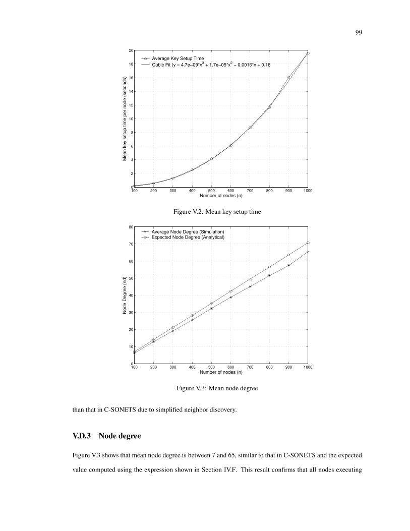
99

100 200 300 400 500 600 700 800 900 10000

2

4

6

8

10

12

14

16

18

20

Number of nodes (n)

Mea

n ke

y se

tup

time

per n

ode

(sec

onds

)

Average Key Setup TimeCubic Fit (y = 4.7e−09*x3 + 1.7e−05*x2 − 0.0016*x + 0.18

Figure V.2: Mean key setup time

100 200 300 400 500 600 700 800 900 10000

10

20

30

40

50

60

70

80

Number of nodes (n)

Nod

e D

egre

e (n

d)

Average Node Degree (Simulation)Expected Node Degree (Analytical)

Figure V.3: Mean node degree

than that in C-SONETS due to simplified neighbor discovery.

V.D.3 Node degree

Figure V.3 shows that mean node degree is between 7 and 65, similar to that in C-SONETS and the expected

value computed using the expression shown in Section IV.F. This result confirms that all nodes executing

100

100 200 300 400 500 600 700 800 900 10001.5

2

2.5

3

3.5

4

4.5

5

5.5

6

6.5

Number of nodes (n)

Mea

n ho

p co

unt t

o a

BS

(h)

Figure V.4: Mean hop-count per node

D-SONETS successfully establish secure pairwise links with their neighbors.

V.D.4 Hop Count

Figure V.4 shows that the mean hop count to a BS follows a decreasing trend, similar to that in C-SONETS,

as network size increases. Hop counts decrease from approximately 7 to 2, as the number of nodes increases

from 100 to 1000. This is an important result because it validates the topology discovery mechanism in D-

SONETS which restricts propagation of information regarding sensor nodes to a limited neighborhood while

ensuring that information regarding routes to BSs propagates unrestricted.

V.D.5 Comparison to existing protocols

DSO/SPKE compares more favorably with existing probabilistic protocols and LEAP in terms of energy con-

sumption. We have observed that at smaller network sizes (i.e., networks with 500 or less nodes), probabilistic

protocols consume (for neighbor discovery and key setup only) approximately one-third of the overall energy

consumed (neighbor discovery, key setup and topology discovery) by DSO/SPKE. Thus, according to Figure

V.1, probabilistic protocols consume approximately 0.1 J to 0.6 J for neighbor discovery and key setup. For

larger networks (i.e., networks with more than 500 nodes), the overall energy consumption of DSO/SPKE

is approximately an order of magnitude higher than probabilistic protocols. According to Figure V.1 would

101

consume approximately 0.3 J to 0.9 J for networks with sizes ranging from 600 to 1000 nodes. Based on

information provided in [61], we infer that D-SONETS and LEAP have similar energy consumption values.

DSO/SPKE exhibits the same kind of properties as SO/SPKE with respect to node degree and hop count.

Therefore, we refer the reader to discussion comparing SO/SPKE and existing protocols with respect to these

two metrics in Section IV.F.5.

V.E Distributed Multi-hop Pairwise Key Establishment (DMPKE)

Because topology discovery is limited to a node’s 2-hop neighborhood, a node can only setup pairwise keys

with 2-hop neighbors when required. Multi-hop pairwise keying between nodes at distances greater than

two hops is accomplished by first establishing a 2-hop pairwise key and subsequently employing the 2-hop

neighbor as a router on the path to the destination

In general, to establish a multi-hop pairwise key with a node ¯ , node a creates its ¼¶H#X�Í¶Ï and transmits it

securely in a FWD message to its router using the pairwise key established between them. The router receives

the message, verifies it and re-transmits it to node ¯ as a SEEDATA message. Node ¯ , in turn, creates ¼¶H#X�Ï�Íand forwards it to node a via the same router. Thus, nodes a and ¯ establish a pairwise key after combining

computing s Í¶Ï as discussed in Section V.B.

The performance of DMPKE was evaluated by simulating a 100-node WSN and verifying correctness

of the protocol. Verification consisted of ensuring that both the source and destination nodes established the

same pairwise key.

V.F Distributed Node Addition

We believe that node addition would be a rare occurrence in WSNs deployed rapidly for purposes such as

those described in the example in Section V.A because such networks would not be required to remain active

for a very long period of time. Further, we assume that adversarial activities against the existing WSN are

detected sufficiently in advance of deploying new nodes, thereby ensuring that actions such as re-keying s �have taken place. Therefore, new nodes are not affected by adversaries in the area of deployment. We also

observe that the adaptability component of our framework, discussed in Chapter II, would also ensure that

node addition occurs at the appropriate security level. Thus, if adversaries are still active in the region of

deployment and nodes can switch between D-SONETS and C-SONETS, then SWANS would ensure that

102

existing nodes employ C-SONETS to allow new nodes into the WSN as opposed to D-SONETS.

New nodes to be added to an existing WSN are pre-loaded with all required information prior to deploy-

ment. Upon deployment, they perform neighbor discovery and key setup. After pairwise key setup, existing

nodes provide the new nodes with both topology and routing information via NLIST and RTINFO messages,

respectively.

The procedure for node addition is the same as DSO/SPKE, except that the neighbor discovery process

is modified. The only modification is that existing non-BS nodes (which are already in the WSN) respond

to HELLO messages from new nodes with HELLO ACK messages. New nodes use source addresses in

HELLO ACK message to discover existing nodes and HELLO messages alone to discover other new nodes

in their neighborhood. Subsequent to neighbor discovery, key setup and topology discovery proceed as

described in Sections V.C.2 and V.C.3, respectively.

Node addition is simulated using 200 nodes. Initially, the WSN is assumed to contain 100 nodes. WSN

size subsequently is increased by adding 10 to 100 nodes in ten separate simulations. Results indicate that

total energy consumption increases from approximately 0.38 J/node (adding 10 nodes) to approximately 0.9

J/node (adding 100 nodes). Increased energy consumption is due to transmission of HELLO ACK messages

repeatedly by a larger set of existing nodes, as the number of nodes added increases from 10 to 100. As

expected, mean node degree ranges from 5 to 12, as the number of nodes added increases from 10 to 100.

The mean hop-count to a BS is approximately 5 hops per node, which is comparable to that reported in Figure

V.4 for DSO/SPKE.

V.G Node Deletion

D-SONETS employs the same protocol to delete misbehaving or compromised nodes as C-SONETS (see

Section IV.I).

V.H Security Analysis

We analyze security aspects of D-SONETS in a manner similar to that of C-SONETS in Section IV.J.

103

V.H.1 Effects of node compromise

Assuming that node compromise is likely after time � � ¹ Í ² , as stated in Section V.B, topology discovery will

be affected. A compromised node could propagate false routing information to its 1-hop neighbors or selec-

tively drop packets containing routing information. These attacks are localized to the 1-hop neighborhood

of the compromised node because of the restricted on propagation of routing information. Further, routing

information from non-compromised nodes in the neighborhood serves to expose the compromised node and

ensure its removal from the network. For example, if a node a receives information from three neighbors ¯ ,× and u that they are 4, 1 and 3 hops away from base station BS1, respectively, then node a can determine

that information provided by × is erroneous. If node × continuous to provide erroneous information, then it

will eventually be deleted from the network.

Node compromise also affects DMPKE as follows. A compromised node a can selectively forward ONS

messages received from its neighbors, which attempt to establish pairwise keys with their 2-hop neighbors via

a . It could also alter and replay ONS messages in order to obtain enough ciphertext to launch cryptanalytic

attacks on the encryption algorithm and as part of a denial-of-service attack. These attacks are local to a ’s

neighborhood.

Distributed node addition is not significantly affected by node compromise because new nodes discover

uncompromised nodes along with any compromised nodes. Thus, using combined information provided by a

larger number of uncompromised neighbors, new nodes can discard spurious information from compromised

nodes (e.g., shorter route to a BS than neighbors or information indicating that the compromised node is a

BS).

The effects of node compromise on node deletion have already been discussed in Section IV.J.1.

Comparison to existing protocols

D-SONETS compares to existing probabilistic protocols and LEAP in the same manner as C-SONETS. D-

SONETS has the same property as C-SONETS that a compromised node can only reveal keys associated

with links it has established and no other keys. Thus, it is more robust than probabilistic protocols, except

random pairwise keying which has the same property as C-SONETS and D-SONETS.

104

V.H.2 Resilience to known attacks

We evaluate the resilience of D-SONETS to Sinkhole, Sybil, Wormhole, HELLO flood attack and node

replication. We assume that the adversary can launch these attacks after �� � ¹ Í ² . Further, we assume that the

adversary can compromise a node and at least obtain s � .Sinkhole attack

In D-SONETS, sensor nodes exchange neighbor lists before advertising the fact that they are in the vicinity

of a BS. The process of exchanging neighbor lists ensures redundancy of information which enables a node

to determine whether a neighbor is being truthful or not and thereby foil a Sinkhole attack by the adversary.

Sybil attack

This attack, when launched after neighbor discovery and key setup, cannot succeed against D-SONETS

because at that point in time each node is aware of the true identity of all its neighbors.

Wormhole attack

This attack cannot succeed against D-SONETS because the neighbor discovery procedure requires a BS to

acknowledge a node’s HELLO message with a secure HELLO ACK message before the latter considers the

former a 1-hop neighbor. Thus, a legitimate node a will never consider distant colluding nodes as neighbors

because its HELLO message will never reach them.

HELLO flood attack

This attack fails during topology discovery when each node observes that the attacker is one hop away from

all its neighbors and their neighbors. This will cause one or more nodes to initiate node deletion of the

attacker from the network.

Node replication

Nodes that are compromised, replicated and deployed elsewhere in the network after �� � ¹ Í ² will fail to

adversely affect legitimate nodes. This is because the compromised nodes do not possess any information

regarding nodes in the new neighborhood including topology and security information. Thus, they will be

unable to communicate with other nodes without being detected and deleted from the network.

105

V.I Chapter Conclusions

This chapter demonstrates a completely distributed protocol suite that employs deterministic pair-wise keying

to achieve security in wireless sensor networks efficiently and in a scalable manner. We have shown that D-

SONETS is applicable to situations rapid deployment of secure WSNs that are resilient to subsequent attacks

by adversaries.

Chapter VI

CONCLUSIONS

Automated monitoring and surveillance mechanisms have been part of our lives for over a decade. Devices

aiding these mechanisms range from tiny accelerometers in automobiles to detect sudden loss of motion to

large video surveillance cameras linked together in malls. The widespread adoption of wireless technologies

and availability of free spectrum has provided a tremendous impetus to the idea of creating devices that

contain tiny sensors along with a microprocessor and a wireless radio, and building large-scale networks of

such devices. The ultimate goal of these wireless sensor networks is to provide the ability to conduct anytime,

anywhere monitoring and surveillance for a fraction of the cost of “wired” sensor networks.

Research in wireless sensor networks has focused on four main areas: energy management, networking,

data management and security. Our study of current literature on wireless sensor network research led us to

conclude that (i) security has not been considered a basic building block in wireless sensor network designs

and (ii) wireless sensor networks do not possess the ability to adapt to the variety of changes that occur in

any environment.

Our research, described in this dissertation, focused on addressing these two issues in wireless sensor

networks and thereby advancing the state-of-the-art of wireless sensor network design. Our thesis was that

a holistic approach to WSN design that provides mechanisms to detect, classify and react to environmen-

tal variations and employs security as a basic building block will result in adaptive WSNs attuned to their

environment thereby improving WSN performance with respect to security, longevity and connectivity.

In order to validate our thesis, we designed and demonstrated a comprehensive framework that consisted

of a two-tiered, ontological framework, SWANS, which ensured that the network would detect, classify and

106

107

respond to a variety of changes in the local environment and a set of security protocol suites, SONETS, to

form the security core of a wireless sensor network.

SWANS is a two-tiered hierarchical component of our framework that ensures both node-level and

network-level adaptability of wireless sensor networks. SWANS employs a comprehensive set of ontolog-

ical descriptions of node and network state reflecting combinations of environmental variations in order to

determine the most appropriate response to an observed variation. We have demonstrated that wireless sen-

sor networks using SWANS can adapt to changes in network topology including addition of new nodes and

failure of existing nodes, and can respond to attacks such as the sleep deprivation torture attack. We have

shown that wireless sensor networks designed using SWANS consume available energy with greater utility

than their non-adaptive counterparts. We have also shown that SWANS is scalable with respect to network

size. Finally, SWANS can also be used as a tool to create environmental descriptions of different complexities

and validate them offline prior to actual deployment on sensor nodes.

P-SONETS is a centralized security protocol suite that secures wireless sensor networks deployed for

perimeter protection. We demonstrated that P-SONETS is well-suited to the class of perimeter protection

applications and can be employed as the security core of a WSN that supports various networking and data

management protocols. C-SONETS extends P-SONETS to provide an efficient, scalable mechanism to secure

wireless sensor networks that can be deployed in a variety of applications. C-SONETS consists of a novel

topology discovery and key setup protocol to ensure that nodes in a heterogeneous wireless sensor network

establish secure links with neighbors. We demonstrated that C-SONETS is scalable with respect to network

size and is resilient to a variety of attacks specific to wireless sensor networks. In order to ensure that sensor

nodes would be able self-organize securely into a resilient wireless sensor network without the need for

trusted computing bases, we designed and evaluated D-SONETS, a completely distributed security protocol

suite. We showed that in situations of reduced threat from adversaries prior to network formation, D-SONETS

ensures rapid formation of a secure wireless sensor network that remains resilient to attacks.

Our framework for secure and adaptive wireless sensor networks can be further enhanced and employed

as a tool for WSN design. We leave these enhancements for future researchers and list them below.

� Enhance the framework with adaptive protocols and mechanisms to improve data fidelity, described in

Section II.B. Thus, the framework would provide adaptivity to variations in application requirements,

data variations and variations in fidelity requirements.

� Develop mapping mechanisms to map sensor data values to ontological symbols, which could then

108

be employed to cause the WSN to improve sensor performance. For example, if the WSN detects an

extreme weather pattern then nodes with sensors able to detect variables associated with that weather

pattern could be instructed to change the sensitivity levels of on-board sensors to record data with

greater frequency.

� Develop a comprehensive policy to include user-defined requirements, external domain information

and observed state information within the network to govern adaptations. This policy would be re-

sponsible for handling complex situations in which data, network and security related adaptations may

conflict with each other. For example, if the adaptation based on data fidelity require nodes to transition

to the sleep state, whereas the security adaptation requires nodes to remain awake, the policy would be

employed to decide the most appropriate adaptation under current conditions.

We also envisage future work on deploying our framework on real-world sensors and evaluating both,

the performance of the WSN and the performance of the framework under a variety of conditions. It is

conceivable that certain aspects of the framework would have to be optimized for deployment on real-world

sensor nodes, given the fact that nodes are resource-constrained with respect to memory and computational

power.

BIBLIOGRAPHY

[1] R. Anderson and M. Kuhn. Tamper Resistance - a Cautionary Note. In Proceedings of the Second

Usenix Workshop on Electronic Commerce, pages 1–11, November 1996.

[2] S. Avancha, A. Joshi, and J. Pinkston. On self-organization and security in distributed wireless sensor

networks. Technical Report TR-CS-04-03, University of Maryland, Baltimore County, July 2004.

[3] S. Avancha, C. Patel, and A. Joshi. Ontology-driven Adaptive Sensor Networks. In Proc. MobiQuitous

2004, pages 194–202, August 2004.

[4] Mote. http://kingkong.me.berkeley.edu/˜nota/RunningMan/Mote.htm. Page from the Smart Dust pro-

gram giving an overview of the Berkeley Renee Mote.

[5] C. Bettstetter. On the Minimum Node Degree and Connectivity of a Wireless Multihop Network. In

Proc. ACM Intern. Symp. on Mobile Ad Hoc Networking and Computing (MobiHoc), pages 80–91,

2002.

[6] R. Blom. An optimal class of symmetric key generation systems. In Advances in Cryptology: Proceed-

ings of EUROCRYPT 84, LNCS, volume 209, pages 335–338. Springer-Verlag, 1985.

[7] C. Blundo, A. D. Santis, A. Herzberg, S. Kutten, and U. Vaccaro. Perfectly-secure key distribution for

dynamic conferences. In Advances in Cryptology - CRYPTO ’92, LNCS 740, pages 471–486, 1993.

[8] P. Bonnet, J. E. Gehrke, and P. Seshadri. Towards Sensor Database Systems. In Proc. of Second

International Conference on Mobile Data Management, January 2001.

[9] N. Bulusu, J. Heidemann, and D. Estrin. Adaptive Beacon Placement. In Proc. ICDCS, 2001.

109

110

[10] D. W. Carman, P. S. Kruus, and B. J. Matt. Constraints and Approaches for Distributed Sensor Network

Security (Final). Technical Report 00-010, NAI Labs, 2000.

[11] H. Chan, A. Perrig, and D. Song. Random key predistribution schemes in sensor networks. In IEEE

Symposium on Research in Security and Privacy, 2003.

[12] G. Chen and B. Szymanski. SENSE: Sensor Network Simulator and Emulator. World Wide Web,

http://www.cs.rpi.edu/˜cheng3/sense.

[13] X. Chen and T. Woo. Energy Efficient Data Encryption Algorithms. World Wide Web:

http://www.vlsi.uwaterloo.ca/˜thwoo/ece750report.pdf, December 2002.

[14] Crossbow Inc. MICA2. www.xbow.com/Products/Product pdf files/Wireless pdf/MICA2 Datasheet.pdf.

[15] J. Deng, R. Han, and S. Mishra. A performance evaluation of intrusion-tolerant routing in wireless

sensor networks. In Proc. of the 2nd International Workshop on Information Processing in Sensor

Networks (IPSN 2003), pages 349–364, April 2003.

[16] D. Denning. Cryptography and Data Security. Addison-Wesley, Boston, MA, 1982.

[17] J. Ding, K. M. Sivalingam, R. Kashyapa, and L. J. Chuan. A Multi-Layered Architecture and Proto-

cols for Large-Scale Wireless Sensor Networks. In Proc. of IEEE Semiannual Vehicular Technology

Conference (VTC), October 2003.

[18] W. Du, J. Deng, Y. Han, and P. Varshney. A Pairwise Key Pre-distribution Scheme for Wireless Sensor

Networks. In Proc. CCS’03, October 2003.

[19] L. Eschenauer and V. D. Gligor. A key-management scheme for distributed sensor networks. In Proc.

of the 9th ACM Conf. on Computer and Communications Security, pages 41–47, November 2002.

[20] O. Goldreich, S.Goldwasser, and S. Micali. How to Construct Random Functions. Journal of the ACM,

33(4):210–217, 1986.

[21] Q. Han, S. Mehrotra, and N. Venkatasubramanian. Energy Efficient Data Collection in Distributed

Sensor Environments. In Proc. of 24th International Conference on Distributed Computing Systems,

pages 590–597, 2004.

[22] T. He, B. M. Blum, J. A. Stankovic, and T. Abdelzaher. AIDA: Adaptive Application-Independent Data

Aggregation in Wireless Sensor Networks. Trans. on Embedded Computing Sys., 3(2):426–457, 2004.

111

[23] W. R. Heinzelman, J. Kulik, and H. Balakrishnan. Adaptive Protocols for Information Dissemination in

Wireless Sensor Networks. In Mobicom ’99, August 1999.

[24] J. Hill, R. Szewczyk, A. Woo, S. Hollar, D. Culler, and K. Pister. System Architecture Directions for

Networked Sensors. In Proc. of ACM ASPLOS IX, November 2000.

[25] V. Hingne, A. Joshi, T. Finin, H. Kargupta, and E. Houstis. Towards a Pervasive Grid. NSF Next

Generation Systems Program Workshop at International Parallel and Distributed Processing Symposium

(IPDPS’ 03), April 2003.

[26] C. Intanagonwiwat, R. Govindan, and D. Estrin. Directed Diffusion: A Scalable and Robust Commu-

nication Paradigm for Sensor Networks. In Proc. of Mobicom ’00, August 2000.

[27] A. Jain and E. Chang. Adaptive Data Sampling for Wireless Sensor Networks. In Proc. International

Workshop on Data Management for Sensor Networks, August 2004.

[28] E. Jovanov, D. Raskovic, J. Price, A. Moore, J. Chapman, and A. Krishnamurthy. Patient Monitoring

Using Personal Area Networks of Wireless Intelligent Sensors. Biomedical Sciences Instrumentation,

37:373–378, 2001.

[29] C. S. Jutla. Encryption Modes with Almost Free Message Integrity. Cryptology ePrint Archive, Report

2000/039, 2000. http://eprint.iacr.org/.

[30] J. Kang, B. Nath, Y. Zhang, and S. Yu. Adaptive Resource Control Scheme to Alleviate Congestion in

Sensor Networks. In Proc. Workshop on Broadband Advanced Sensor Networks, October 2004.

[31] C. Karlof and D. Wagner. Secure Routing in Sensor Networks: Attacks and Countermeasures. In Proc.

of First IEEE International Workshop on Sensor Network Protocols and Applications, May 2003.

[32] O. Kommerling and M. G. Kuhn. Design Principles for Tamper-Resistant Smartcard Processors. In

Proc. of the USENIX Workshop on Smartcard Technology (Smartcard ’99), pages 9–20. USENIX As-

sociation, May 1999.

[33] Y. Kostov and G. Rao. Low Cost Optical Instrumentation for Biomedical Measurement. J. Review of

Scientific Instruments, pages 4361–4373, December 2000.

[34] B. Krishnamachari, D. Estrin, and S. B. Wicker. Modeling Data-Centric Routing in Wireless Sensor

Networks. Technical Report CENG 02-14, Dept. of Computer Engineering, USC, 2002.

112

[35] J. Kulik, W. R. Heinzelman, and H. Balakrishnan. Adaptive Protocols for Information Dissemination in

Wireless Sensor Networks. In Proc. of Mobicom ’99, Seattle, WA, August 1999.

[36] T.-H. Lin, H. Sanchez, H. Marcy, and W. Kaiser. Wireless Integrated Network Sensors (WINS) for

Tactical Information Systems. In Proc. of the Government Microcircuit Applications Conference, 1998.

[37] D. Liu and P. Ning. Establishing pairwise keys in distributed sensor networks. In Proc. of the 10th ACM

Conf. on Computer and Communications Security, October 2003.

[38] S. Madden and M. J. Franklin. Fjording the Stream: An Architecture for Queries over Streaming Sensor

Data. In Proc. of ICDE 2002, February 2002.

[39] S. R. Madden, M. J. Franklin, J. M. Hellerstein, and W. Hong. TAG: A Tiny AGgregation Service for

Ad-Hoc Sensor Networks. In Proc. of Fifth Symposium on Operating Systems Design and Implementa-

tion (USENIX - OSDI ’02), December 2002.

[40] A. Mainwaring, J. Polastre, R. Szewcyzk, D. Culler, and J. Anderson. Wireless Sensor Networks for

Habitat Monitoring. In Proc. WSNA’02, September 2002.

[41] D. L. McGuinness and F. van Harmelen Ed. Web Ontology Language (OWL): Overview. World Wide

Web – http://www.w3c.org/TR/owl-features.

[42] V. Mhatre and C. Rosenberg. Homogeneous vs. Heterogeneous Sensor Networks: A Comparative

Study. In Proc. of IEEE International Conference on Communications, volume 6, pages 3646–3651,

June 2004.

[43] National Institute of Standards and Technology. FIPS 81; DES Modes of Operation, December 1980.

[44] National Institute of Standards and Technology. FIPS 46-2; Data Encryption Standard, December

1993.

[45] The Network Simulator. http://www-mash.berkeley.edu/ns, 1996.

[46] S. Park, A. Savvides, and M. B. Srivastava. Sensorsim: A Simulation Framework for Sensor Networks.

In Proc. of ACM MSWiM 2000, pages 104–111, August 2000.

[47] A. Perrig, J. Stankovic, and D. Wagner. Security in Wireless Sensor Networks. Communications of the

ACM, 47(6):53–57, June 2004.

113

[48] A. Perrig, R. Szewczyk, V. Wen, D. Culler, and J.D.Tygar. SPINS: Security Protocols for Sensor

Networks. Wireless Networks, 8:521 – 534, 2002.

[49] N. R. Potlapally, S. Ravi, A. Raghunathan, and N. K. Jha. Analyzing the energy consumption of security

protocols. In Proc. of ISLPED’03, August 2003.

[50] P. Rogaway, M. Bellare, and J. Black. OCB: A block-cipher mode of operation for efficient authenticated

encryption. ACM Trans. Inf. Syst. Secur., 6(3):365–403, 2003.

[51] B. Schneier. Applied Cryptography. John Wiley & Sons, Inc., 1996.

[52] C. Schurgers, V. Tsiatsis, and M. B. Srivastava. STEM: Topology Management for Energy Efficient

Sensor Networks. In Proc. IEEE Aerospace Conference, volume 3, pages 1099–1108, March 2002.

[53] A. T. Sherman and D. A. McGrew. Key establishment in large dynamic groups using one-way function

trees. IEEE Transactions on Software Engineering, 29(5):444–458, May 2003.

[54] N. Shrivastava, C. Buragohain, D. Agrawal, and S. Suri. Medians and Beyond: New Aggregation

Techniques for Sensor Networks. In Proc. of 2nd International Conference on Embedded Networked

Sensor Systems, pages 239–249, 2004.

[55] A. Sobeih, W. Chen, J. C. Hou, L.-C. Kung, N. Li, H. Lim, H.-Y. Tyan, and H. Zhang. J-Sim:

A Simulation and Emulation Environment for Wireless Sensor Networks. WWW – http://www.j-

sim.org/v1.3/sensor/JSim.pdf.

[56] F. Stajano and R. Anderson. The resurrecting duckling: Security issues for ad-hoc wireless networks.

Lecture Notes in Computer Science, 1796, 1999.

[57] M. Valenti. Smart Sensors – A Technology Assessment Impact (Technical Insights). Technical report,

Frost & Sullivan, September 2004.

[58] T. van Dam and K. Langendoen. An Adaptive Energy-Efficient MAC Protocol for Wireless Sensor

Networks. In Proc. ACM SenSys, November 2003.

[59] Y. Yao and J. E. Gehrke. The Cougar Approach to In-Network Query Processing in Sensor Networks.

SIGMOD Record, 31(3):9–18, September 2002.

114

[60] X. Yu, K. Niyogi, S. Mehrotra, and N. Venkatasubramanian. Adaptive Target Tracking in Sensor Net-

works. In Proc. The 2004 Communication Networks and Distributed Systems Modeling and Simulation

Conference, January 2004.

[61] S. Zhu, S. Setia, and S. Jajodia. LEAP: Efficient security mechanisms for large-scale distributed sensor

networks. In Proc. of the 10th ACM Conf. on Computer and Communications Security, October 2003.