approval sheet - umbc ebiquity research groupebiquity.umbc.edu/get/a/publication/588.pdf ·...

2

APPROVAL SHEET

Title of Thesis: Community Detection in Twitter Name of Candidate: Mohit Naresh Kewalramani Master of Computer Science, 2011 Thesis and Abstract Approved: Dr. Tim Finin Professor Department of Computer Science and Electrical Engineering

Date Approved: ________________

Curriculum Vitae

Name: Mohit Naresh Kewalramani. Permanent Address: 4757 Daryton Green, Baltimore, MD-21227. Degree and date to be conferred: Masters in Computer Science, May 2011. Date of Birth: 03/04/1988. Place of Birth: Dubai. Secondary education: Jai Hind Junior College, Pune, India, 2005. Collegiate institutions attended: University of Maryland Baltimore County, M.S. in Computer Science, 2011. University of Pune, B.E. in Computer Engineering, 2009. Major: Computer Science. Professional positions held: Susquehanna International Group LLP, PA, USA (June 2010 – August 2010).

4

ABSTRACT

Title of Document: COMMUNITY DETECTION IN TWITTER Mohit Naresh Kewalramani

M.S., 2011 Directed By: Dr. Tim Finin, Professor

Department of Computer Science and Electrical Engineering

Twitter has recently evolved into a source of social, political and real time

information in addition to being a means of mass-communication and marketing. Monitoring

and analyzing information on Twitter can lead to invaluable insights, which might otherwise

be hard to get using conventional media resources. An important task in analyzing highly

networked information sources like twitter is to identify communities that are formed. A

community on twitter can be defined as a set of users that have more links within the set than

outside it.

We present a technique to devise a similarity metric between any two users on twitter

based on the similarity of their content, links and metadata. The link structure on Twitter can

be characterized using the twitter notion of followers, being followed and the @Mentions,

@Reply and @RT tags in tweets. Content similarity is characterized by the words in the

tweets combined with the hash-tags they are annotated with. Meta-data similarity includes

similarity based on other sources of user information such as location, age and gender. We

then use this similarity metric to cluster users into communities using spectral and bottom-up

agglomerative hierarchical clustering. We evaluate the performance of clustering using

different similarity measures on different types of datasets. We also present a heuristic to find

communities in twitter that take advantage of the network characteristics of twitter.

COMMUNITY DETECTION IN TWITTER

By

Mohit Naresh Kewalramani

Thesis submitted to the Faculty of the Graduate School of the University of Maryland, Baltimore County, in partial fulfillment

of the requirements for the degree of Master of Science

2011

6

© Copyright by Mohit Naresh Kewalramani

2011

ii

Dedicated to Mummy, Papa and Richa

iii

Acknowledgements

I would like to express my sincere gratitude to my graduate advisor Dr. Tim Finin. I

would like to thank him for his constant support and continued belief in me. His

suggestions, motivation and advice were vital in bringing this work to completion. I

would also like to thank Dr. Anupam Joshi and Dr. Tim Oates for guiding me

whenever I needed guidance and for graciously agreeing to be on my thesis

committee.

I would also like to thank all my friends for their constant encouragement during my

academic life at UMBC.

iv

Table of Contents

Dedication .................................................................................................................... ii

Acknowledgements .................................................................................................... iii

Table of Contents ........................................................................................................ iv

List of Tables ............................................................................................................. vii

List of Figures .......................................................................................................... viii

Chapter 1: Introduction .............................................................................................. 1

1.1 Social Media ....................................................................................................... 1

1.2 Twitter ................................................................................................................ 2

1.3 Communities in Social Media ........................................................................... 5

1.4 Motivation .......................................................................................................... 6

1.4.1 Politics .......................................................................................................... 7

1.4.2 Brands and Advertisements ....................................................................... 8

1.4.3 Sports ........................................................................................................... 8

1.5 Thesis Contribution ........................................................................................... 9 Chapter 2: Background and Related Work ............................................................ 11

2.1 Background ...................................................................................................... 11

2.1.1. Clustering ................................................................................................. 11

2.2 Related Work ................................................................................................... 15

2.2.1 Communities in Social Network .............................................................. 15

Chapter 3: System Design and Implementation ..................................................... 17

3.1 System Design .................................................................................................. 17

v

3.2 Tweet Collection .............................................................................................. 17

3.2.1 Twitter API and Twitter4J Java Library .............................................. 18

3.2.2 Parameters ................................................................................................ 18

3.3 Database ........................................................................................................... 19

3.4 Similarity Metrics ............................................................................................ 20

3.4.1 Content Similarity .................................................................................... 20

3.4.2 Link Similarity .......................................................................................... 21

3.4.3 Metadata .................................................................................................... 26

3.5 Clusters ............................................................................................................. 29

3.5.1 N-Cuts ..................................................................................................... 29

3.5.2 Bottom-Up Agglomerative Clustering .................................................... 31

3.5.3 Bottom-Up Fusing Heuristic .................................................................... 32

Chapter 4: Results ..................................................................................................... 39

4.1 Datasets ............................................................................................................. 39

4.1.1 India-Pakistan Cricket World Cup Semi-Final Tweets ........................ 39

4.1.2 Democrat-Republic Tweets ...................................................................... 39

4.1.3 Indian Premier League Tweets ............................................................... 40

4.1.4 iPhone-Android Tweets ............................................................................ 41

4.1.5 Tweets Pertaining to Different Universities in Maryland ..................... 42

4.2 Definitions ........................................................................................................ 42

4.2.1 Rand Index ................................................................................................ 42

4.2.2 Modularity Score ...................................................................................... 43

4.3 Cluster Validation ........................................................................................... 43

vi

4.3.1 N-Cuts ........................................................................................................ 43

4.3.2 Bottom-Up Agglomerative Hierarchical ................................................ 48

Chapter 5: Conclusion and Future Work .............................................................. 56

5.1 Conclusion ........................................................................................................ 56

5.2 Future Work .................................................................................................... 57 Bibliography ............................................................................................................... 58

vii

List of Tables Table 4.1 Statistics for India-Pakistan CWC Semi-Final Dataset ............................... 39

Table 4.2 Statistics For Democrat-Republic Dataset .................................................. 40

Table 4.3 Statistics For IPL Dataset ............................................................................ 41

Table 4.4 Statistics For Cricket-Soccer Dataset .......................................................... 41

Table 4.5 Statistics for Universities in Maryland Dataset ........................................... 42

Table 4.6 N-Cuts: Content Similarity .......................................................................... 44

Table 4.7 Most Common Words ................................................................................. 45

Table 4.8 Most Common Hashtags ............................................................................. 45

Table 4.9 Most Common Words ................................................................................. 46

Table 4.10 Most Common Hashtags ........................................................................... 46

Table 4.11 N-Cuts: Link Similarity ............................................................................. 47

Table 4.12 N-Cuts: Content, Link & Metadata Similarity .......................................... 48

Table 4.13 Bottom-Up Agglomerative Hierarchical: India-Pakistan CWC Semi-Final

............................................................................................................................. 50

Table 4.14 Bottom-Up Agglomerative Hierarchical: Democrat-Republic Dataset .... 51

Table 4.15 Bottom-Up Agglomerative Hierarchical: IPL ........................................... 53

Table 4.16 Bottom-Up Fusing Heuristic: India-Pakistan CWC Semi-Final ............... 54

Table 4.17 Bottom-Up Fusing Heuristic: Democrat-Republic Dataset ....................... 54

Table 4.18 Bottom-Up Fusing Heuristic: IPL Dataset ................................................ 55

viii

List of Figures

Figure 1.1 Number of Twitter Users (Figure Courtesy Twitdir) ................................... 3 Figure 1.2 An Example of Communities ....................................................................... 5 Figure 1.3 An Example of Communities with One Node Shared Between Two

Communities .......................................................................................................... 6 Figure 1.4 Political Twitter Accounts With Most Followers (Figure Courtesy

www.sysomos.com) .............................................................................................. 7 Figure 1.5 Volume of Tweets on Super Bowl Sunday as Compared to The Previous

Sunday (Figure Courtesy Twitter Blog) ................................................................ 8 Figure 2.1 Dendrogram Representation for Hierarchical Clustering (Figure Courtesy:

Wikipedia) ........................................................................................................... 12 Figure 2.2 Demonstration of k-means Clustering (Figure Courtesy: Wikipedia) ....... 13 Figure 3.1 System Architecture ................................................................................... 17 Figure 3.2 Tweet Collection ........................................................................................ 17 Figure 3.3 Database Schema ....................................................................................... 19 Figure 3.4 Hashtags in Twitter .................................................................................... 21 Figure 3.5 Retweets in Twitter .................................................................................... 22 Figure 3.6 Replies in Twitter ....................................................................................... 23 Figure 3.7 An Example of Mentions in Twitter .......................................................... 24 Figure 3.8 Twitter Users With Location (Figure Courtesy: www.sysomos.com) ....... 27 Figure 3.9 Flowchart - Location Similarity ................................................................. 29 Figure 3.10 Tweets Posted (Figure Courtesy: www.sysomos.com) ........................... 33 Figure 3.11 Degree of Separation in Twitter Graph (Figure Courtesy:

www.sysomos.com) ............................................................................................ 34 Figure 3.12 Determination of Seeds of the Graph ....................................................... 34

ix

Figure 3.13 Finding The Immediate Neighborhood of Each Seed .............................. 35 Figure 3.14 Fuse Clusters With Common Users ......................................................... 36 Figure 3.15 Resolve Users That Belong to More Than One Community ................... 37 Figure 3.16 Repeat Until Terminal Condition is Reached .......................................... 37 Figure 4.1 N-Cuts: Content Similarity ........................................................................ 44 Figure 4.2 N-Cuts: Link Similarity ............................................................................. 47 Figure 4.3 N-Cuts: Content, Link & Metadata Similarity ........................................... 48 Figure 4.4 Bottom-Up Agglomerative Hierarchical: India-Pakistan CWC Semi-Final

............................................................................................................................. 49 Figure 4.5 Bottom-Up Agglomerative Hierarchical: Democrat-Republic Dataset ..... 50 Figure 4.6 Bottom-Up Agglomerative Hierarchical: IPL Dataset ............................... 52 Figure 4.7 Bottom-Up Fusing Heuristic: India-Pakistan CWC Semi-Final ................ 53 Figure 4.8 Bottom-Up Fusing Heuristic: Democrat-Republic Dataset ....................... 54 Figure 4.9 Bottom-Up Fusing Heuristic: IPL Dataset ................................................. 55

1

Chapter 1: Introduction

In this chapter we present an introduction to the online social media and twitter. We

will discuss the use of twitter in social, commercial and political environments. We show the

motivation clustering the data in these environments and present a formal thesis definition.

1.1 Social Media

Social Media has recently evolved into a source of social, political and real time

information in addition to being a means of communication and marketing. Status updates,

blogging, sharing videos and images, forming groups and communities are some of the ways

people use to share and spread information. Monitoring and analyzing this information can

lead to valuable insights that might otherwise be hard to get using conventional methods and

media sources. ��

The rapid advent of social networking sites has changed the way people receive and

share information and knowledge and also communicate with each other. The ability to

embed metadata in the form of links, images and videos means that social Networking sites

are an important source of information for people not only about their friends but also about

their immediate and distant surrounding. Sites like Twitter, Facebook, blogs, Wikipedia,

Flickr and YouTube are a few examples that have emerged as a major source of information

for most of the world wide web users. Advertisers, political campaigning activists and data

miners have started studying and successfully using social networks and the network of

interactions and information therein to analyze the spread of ideas, social relationships and

viral marketing.

Conventional media only allowed users to gain information as was provided to

them. Transfer of information only took place in one direction i.e. from the source to the

users. They could not respond to the news, provide their opinion and share it. The new social

2

networking platforms have given users the power to share information, gain and add to

information posted by other users as well as spread information over their social network.

This has led to the evolution of a multi-way mode of information dissemination in which the

users are not allowed to post and spread information in addition to metadata in the form of

links, images and video. As a result, the formation of a user-generated model of information

dissemination in which the social graph of the user plays an important role in determining the

mode and rate at which information is spread. This vast amount of “user generated content”

generated everyday is an important source of information which can be used to gain

numerous inferences.

Micro-blogging1 websites such as Facebook1, Orkut2 and Twitter3 allow users to

post short status messages on their homepage. These websites are an instant source of

information about popular social, political, environmental events as well as general public

perception and sentiment. The short messages users post are often called ‘status updates’.

Status updates in Twitter are more commonly called as tweets. Tweets are often related to

some event, specific topic of interest like music, dance or personal thoughts and opinions. A

tweet can contain text, emoticon, link or a combination of them.

1.2 Twitter

Twitter is a fast expanding, free and a very quick social network that has emerged as

a major source of information. Twitter is a micro-blogging social networking website that

started in March 2006 and has amassed more than 75 million users as on Feb 20114 and is

expanding extremely fast. It is also ranked number 20 in popularity among all social

networking sites globally and is ranked as the most popular micro-blogging website (Hughes

1 www.facebook.com 2 www.orkut.com 3 www.twitter.com 4 www.twitdir.com

3

A. L.).

Figure 1.1 Number of Twitter Users (Figure Courtesy Twitdir)

Twitter allows its users to post and share short messages up to 140 characters in

length with other twitter users. These status messages are called ‘tweets’. Tweets can be

posted or ‘tweeted’ through a vast variety of media, which includes text messaging, the

internet, instant messaging, smart phone applications and a wide variety of other third party

applications. Users may choose to share their tweets publicly with anyone, or restrict access

to their tweets so that only users they give permission may view them. Replying to tweets,

mentioning other users in tweets and spreading tweets have lead to a well-defined mark-up

culture. Users can reply to tweets by prefixing the tweet by ‘@’ followed by the user they are

replying to. Users can be mentioned in tweets by adding ‘@’ followed by the users twitter

screen name anywhere within the tweet. Spreading interesting and popular tweets is called

retweeting and is done by prefixing the tweet to be spread by ‘RT @’ followed by the

username of the user whose tweet is retweeted. Retweeting is an important tool that users

virally spread information over twitter. Users can also tag their tweets using hashtags ie by

inserting ‘#’ followed by the tag in their tweet.

4

A special characteristic of twitter is that as opposed to most other sites like facebook

and orkut, the relationship of following and being followed is not necessarily two ways. In

fact in most of the cases it applies only in one direction ie one user follows another and the

other user does not follow the first one back. Following someone is equivalent to subscribing

to a blog. A user that follows someone receives all the tweets of the person he follows.

As a twitterer can post status messages using applications on their smart phones and

also using text messages, twitter has risen as an important source of real time information in a

variety of situations including sports events, mass emergencies and crisis events. In October

2007 twitter was employed to quickly inform citizens about critical information such as road

block, safety measures, evacuations and shifts in fire lines. It was also used in Mumbai during

the terror attacks on Hotel Taj on November 27th 2008 (Stelter B.) to provide real time

updates. Besides twitter has been used for predicting box office performances of movies,

predicting election results etc. Twitter’s growing popularity makes it important to analyze the

content in twitter so that it can be efficiently utilized during such situations.

A key characteristic of twitter is its underlying “Social Graph”. Individuals can

discover and post information, share their opinions and “” using this social graph. A social

graph can be described as the sum of all declared social relationships across the participants

in a given network. Studying the structure and characteristics of this graph in twitter about a

topic or occurrence can give us a huge amount of important information.

Twitter users tend to cluster around each other based factors like common interests, similar

affiliations, opinions and geography. Identifying communities amongst twitter users in an

important task that leads to wide range of useful information. A community in twitter’s social

graph can be described as a subset of the social graph with more links within it than outside

it. Links could be anything from a user mentioning, replying or retweeting another users

tweet to similarities between users based on geography, words and hashtags used etc.

5

1.3 Communities in Social Media

An important practical problem in social networks is to discover communities of

users based on their content and relationships with other users. A community is a pattern with

dense links internally and sparse links externally. These links can be characterized by the

content similarity between users, friendship between them and also other similarities in their

personal data such as their location, gender, age etc. These close structures can then be used

for various purposes such as targeting marketing schemes, terrorist cells.

Figure 1.2 An Example of Communities

The social links of friendship is an important part of most social networks. These

social links often give rise to communities i.e. subsets of users represented as vertices within

which connections are dense put between which connections are relatively sparse. A sketch

of a community is shown in fig 1.2. The nodes 1,2,3 and 4 form one community whereas the

nodes 5,6,7 and 8 form another community. Communities in a social network might represent

real social groupings, perhaps by interest or background being able to identify these

communities could help us to understand and exploit these networks more effectively. The

ability to detect community structure in a network could clearly have practical applications.

6

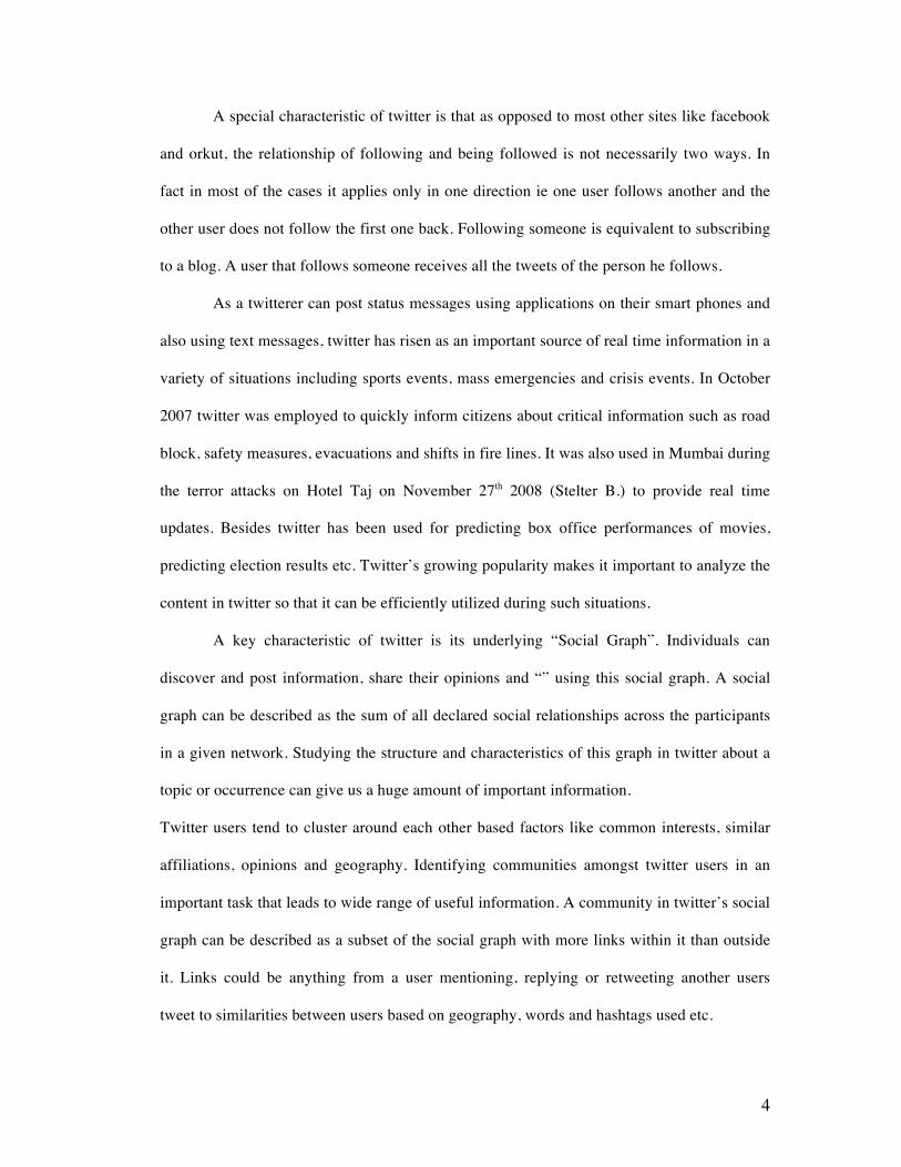
Figure 1.3 An Example of Communities with One Node Shared Between Two Communities

Most of the existing approaches for community detection are based on link analysis

and ignore the vast amount of other information available in most new age social networks.

Besides most community detection algorithms have cubic time complexity in the number of

nodes. They also divide nodes into unique clusters. This is definitely not true of social

networks. In social networks like Facebook and Twitter one user can be a part of more than

one cluster. Besides twitter has different types of links in the form of follower-following

relationships, retweets, mentions and replies. Tweets also contain hashtags and links with

images and videos. Additionally, Twitter provides a lot of metadata in the form of user

location, interests, age and gender that can be used for clustering.

We present a technique to analyze and combine all these sources of information and

evaluate two major clustering techniques in twitter. We also propose a bottom-up fusing

technique, which efficiently makes use of all the links and meta-data present in twitter to

form clusters.

1.4 Motivation

Twitter has evolved as a source of real-time information for corporate brands,

advertisers and situation analysts. In this sub-section we describe how twitter can be a useful

source of information in a variety of situations.

7

1.4.1 Politics

Twitter was used extensively in the last U.S. presidential campaign when Barack

Obama’s enthusiastic use of social media made a big impact on the use of social media in

politics. Twitter presents the politician a user-friendly platform where they can talk about

political issues and have a huge and relevant audience. In addition to President Obama, high-

profile politicians in Twitter include Hilary Clinton, California Governor Arnold

Schwarzenegger, U.S. Senator Jim DeMint, British Prime Minister Gordon Brown and

Canadian Prime Minister Stephen Harper. (http://www.sysomos.com)

Political communities can be detected within tweets of an election campaign. These

communities can then be analyzed to see what supporters of various candidates are tweeting

about. These communities are an invaluable source of information for political campaign

analysts.

Figure 1.4 Political Twitter Accounts With Most Followers (Figure Courtesy www.sysomos.com)

8

1.4.2 Brands and Advertisements

The huge wealth of information present in twitter contains priceless intelligence and

knowledge for advertisers, marketers and other big corporate brands. Corporate companies

have always accumulated information about their customers that helps them to market their

products better.

Communities within this domain of tweets can be analyzed to figure out influential

tweeters about specific brands, products and technologies. The spread of information from

these information-broadcasting users can then be analyzed to figure out improvements and

better marketing strategies for products and technologies.

1.4.3 Sports

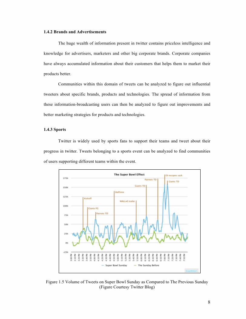
Twitter is widely used by sports fans to support their teams and tweet about their

progress in twitter. Tweets belonging to a sports event can be analyzed to find communities

of users supporting different teams within the event.

Figure 1.5 Volume of Tweets on Super Bowl Sunday as Compared to The Previous Sunday (Figure Courtesy Twitter Blog)

9

1.4.4 Disaster Events and Mass Emergencies

Twitter has emerged as an important source of real-time information during disaster-

events and mass-emergencies. The flexibility and mobility of twitter makes it easy to post

updates through twitter during such situations. News agencies and other users through twitter

update updates about the current on-the-ground situation, relief efforts and other important

news. In late October 2007, instances of Twitter use in the diffuse Southern California US

wildfires to inform citizens of time-critical information about road closures, community

evacuations, shifts in fire lines, and shelter information suggested its more purposeful and

widespread use in the future (Sutton J.). More recently, Twitter was used by those in the area

of effect to report on the events that took place in the Mumbai, India terrorist attacks on

November 26, 2008 (Stelter B.).

Detection of communities can be applied on such domains to analyze and get a

bigger picture of the local situation. Influential users within communities can be found out

and can be used to distribute information quickly and efficiently.

1.5 Thesis Contribution

The thesis contribution can be briefly stated as

• We define a similairity metric between any two users based on their content

similarity, link similarity and meta-data similarity. We calculate content similarity

based on word and hash-tag similarity. Link similarity is calculated based on the

follower-following relationship between two users and the number of times they have

retweeted, mentioned or replied to each other. Meta-data similarity is determined

based on similarity of meta-data such as location, gender and age.

• We cluster twitter users into communities using spectral clustering and bottom-up

agglomerative hierarchical clustering. We also present a bottom-up fusing heuristic to

find communities that takes advantage of some of the characteristics of the twitter

10

network. We analyze the accuracy of the clustering using rand index and silhouette

index.

• We show that the effectiveness of similarity metrics based on link similarity remain

constant across various tweet domains. Performance of word similarity and meta-data

similarity are dependent upon the kind of tweets being clustered.

11

Chapter 2: Background and Related Work

2.1 Background

2.1.1. Clustering

Clustering is the process of taking collections of objects such as tweets and

organizing them into groups based on their similarity. These groups are called as clusters.

Following are the two main types of clustering algorithm:

1. Hierarchical Clustering Algorithm (Newman, Detecting Community Structure in

Network)

There are further two types of this algorithm:

i. Agglomerative Clustering: This clustering algorithm uses the bottom-up

approach. These algorithms have input as each individual document, which is

considered as a separate cluster of size one. Each level consists of merging of

smaller clusters to form the bigger cluster and the process ends when all the

clusters are merged into a single cluster that contains all the documents.

ii. Divisive Clustering: This clustering algorithm uses the top-down approach.

These algorithms begin with entire set and further splitting generates

successive smaller clusters. The recursive implementation continues till

individual documents are reached.

Information retrieval is more frequently done using Agglomerative

Clustering over Divisive Clustering. A greedy algorithm is used to make the splits

and merges. A greedy algorithm follows a problem solving heuristic by which a

locally optimum choice is made at each stage with a hope of finding a global

optimum. The results are depicted using a dendrogram as shown in figure below.

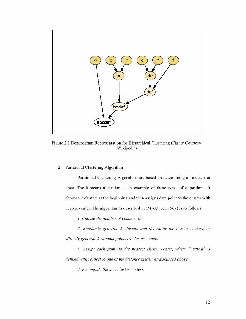
12

Figure 2.1 Dendrogram Representation for Hierarchical Clustering (Figure Courtesy: Wikipedia)

2. Partitional Clustering Algorithm

Partitional Clustering Algorithms are based on determining all clusters at

once. The k-means algorithm is an example of these types of algorithms. It

chooses k clusters at the beginning and then assigns data point to the cluster with

nearest center. The algorithm as described in (MacQueen 1967) is as follows:

1. Choose the number of clusters, k.

2. Randomly generate k clusters and determine the cluster centers, or

directly generate k random points as cluster centers.

3. Assign each point to the nearest cluster center, where "nearest" is

defined with respect to one of the distance measures discussed above.

4. Recompute the new cluster centers.

7

FIG. 2.2. Dendrogram representation for hierarchical clustering (figure courtsey:Wikipedia)

2.2.2 Partitional clustering algorithms

Partitional clustering algorithms typically determine all clusters at once. The k-means

clustering algorithm belongs to this category. It starts off with choosing ’k’ clusters and

then assigning each data point to the cluster whose center is nearest. The algorithm as

described in (MacQueen 1967) is as follows:

1. Choose the number of clusters, k.

2. Randomly generate k clusters and determine the cluster

centers, or directly generate k random points as

cluster centers.

3. Assign each point to the nearest cluster center, where

"nearest" is defined with respect to one of the

distance measures discussed above.

4. Recompute the new cluster centers.

5. Repeat the two previous steps until some convergence

criterion is met (usually that the assignment

hasn’t changed).

13

5. Repeat the two previous steps until some convergence criterion is met

(usually that the assignment hasn’t changed).

Figure 2.2 Demonstration of k-means Clustering (Figure Courtesy: Wikipedia)

The k-means algorithms show their significance in their simplicity and speed

when applied to large datasets. The complexity of most common hierarchical

clustering algorithms is found to be at least quadratic in the number of documents as

compared to the linear complexity of k-means algorithms. K-means is linear in all

relevant factors such as iterations, number of clusters, number of vectors and

dimensionality of the space. This specifies that k-means is more efficient than

hierarchical clustering algorithms as described in (Manning, Raghavan, & Schutze

2008).

3. Spectral Bisection (Newman, Detecting Community Structure in Network)

For an n-vertex undirected graph G the Laplacian is defined as an n x n

symmetric matrix L. The diagonal element Lii of the symmetric matrix L is the

degree of the vertex i whereas the off diagonal element Lij is one less if the

8

FIG. 2.3. Demonstration of k-means clustering (figure courtsey: Wikipedia)

The main advantages of k-means are its simplicity and speed when applied to large

data sets. The most common hierarchical clustering algorithms have a complexity that is

at least quadratic in the number of documents compared to the linear complexity of k-

means. K-means is linear in all relevant factors: iterations, number of clusters, number of

vectors and dimensionality of the space. This means that k-means is more efficient than the

hierarchical algorithms as described in (Manning, Raghavan, & Schutze 2008). Figure 2.3

gives a demonstration for a k-means algorithm.

2.3 Related Work

Topic models have been applied to a number of tasks that are relevant to our goal of

clustering Twitter status messages. We will briefly describe three categories and cite a few

examples in each.

2.3.1 Topic models for information discovery

There has been some work with regards to using topic models for information discov-

ery. (Phan, Nguyen, & Horiguchi 2008) presents a framework to build classifiers using both

a set of labelled training data and hidden topics discovered from large scale data collections.

14

vertices i and j are connected and zero otherwise. Thus L can also be written as L

= D – A where D is the diagonal matrix of vertex degrees and A is the adjacency

matrix. Now as the degree at a particular vertex in diagonal matrix D is given by

an equation Dii = Σj Aij it specifies that the Laplacian matrix has the rows and

columns all summing to zero. This further specifies that the vector 1 = (1, 1, 1,

…) is always an eigenvector with value zero. The separation of the network into

communities depicts the appearance of the Laplacian as follows:

1. If the network is separated perfectly into communities such that the graph

contains only ‘within-community’ edges and not the ‘between-community’

ones then the Laplacian will be block diagonal. The Laplacian of a diagonal

block will be formed by itself and thus has an eigenvector v(k) with

eigenvalue zero. Hence there will be g eigenvectors with eigenvalues 0.

2. If the network is separated well nut not perfectly separated into communities

then the Laplacian will not be a block diagonal. Instead there will be one

eigenvector 1 with eigenvalue zero and g – 1 eigenvalues slightly different

from zero. The corresponding eigenvectors are the linear combination of v(k) .

Hence by looking at the eigenvalues of the graph Laplacian only slightly

greater than zero and taking their linear combination of the corresponding

eigenvectors one should be able to find the blocks themselves.

Thus we can divide the network into its two communities by looking at the

eigenvector corresponding to the second lowest eigenvalue and separating the

vertices by whether the element is greater than or less than zero. This is the way

the spectral bisection method works. It gives better results in cases where the

graph really splits nicely into two communities. The second eigenvalue λ2 is

called algebraic connectivity of the graph.

15

2.2 Related Work

2.2.1 Communities in Social Network

A network or graph can be represented as a set of points, or vertices, joined

in pairs by lines, or edges. Communities emerge in many types of networks. A

community in a graph is defined as a subset of vertices that are densely connected

with each other and sparsely connected with other vertices in the graph. The study of

the underlying properties of communities in networks has interested researchers for

many years.

Most of the existing approaches to community detection are based on link

analysis and ignore the folksonomy meta-data that is easily available on in social

media. Java et al. (Akshay Java A. J.) present a novel method to combine the link

analysis for community detection with information available in tags and

folksonomies, yielding more accurate communities. They also present an

approximation method by sampling a small portion of the graph in order to

approximately determine the overall community structure.

Girman and Newman (M. Girvan) presented a general community detection

algorithm which requires computation of “edge betweenness centrality” which is an

expensive measure. Newman provides a fast approximation to this measure. Shi and

Malik (Malik) present a technique called N-Cuts which requires calculating the

second eigenvector of the similarity matrix called the Fiedler or the connectivity

vector and then using this vector to repeatedly bisection the graph. Kenighan and Li[]

presented a heuristic to find communities by repeated bisection of the initial graph.

Not all communities are static in nature. Communities can be considered to

be dynamic with respect to shifts in interests, temporal factors and reaction of

community members to news and events. Communities may dynamically split or

16

merge to form smaller or bigger communities. Chi et al.[] present a technique to

extend spectral clustering algorithms for social networks and blogs that evolve over

time.

17

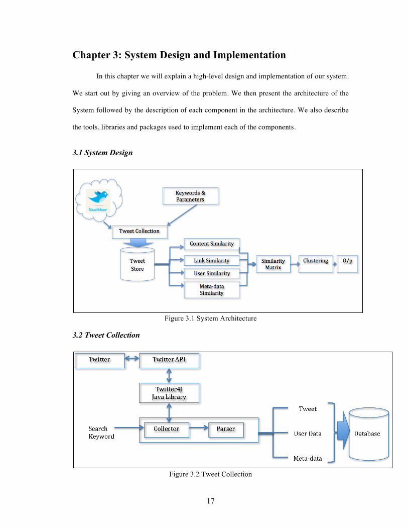
Chapter 3: System Design and Implementation

In this chapter we will explain a high-level design and implementation of our system.

We start out by giving an overview of the problem. We then present the architecture of the

System followed by the description of each component in the architecture. We also describe

the tools, libraries and packages used to implement each of the components.

3.1 System Design

Figure 3.1 System Architecture

3.2 Tweet Collection

Figure 3.2 Tweet Collection

18

3.2.1 Twitter API and Twitter4J Java Library

Twitter4J is an open-sourced, mavenized and Google App Engine safe Java

library for the Twitter API which is released under the BSD license. We have used it

to collect tweets using its streaming and search methods implementation from the

twitter4j package.

3.2.2 Parameters

1. Input

The tweet collector takes ‘search queries as input’. It then uses twitter4j’s

streaming libraries to search twitters live stream for the keywords. The keywords

can be ORed or ANDed together as required.

2. Output

The output of the tweet collector includes tweets which has the search keyword

as a part of its text in addition to the following.

a. Tweet Id

b. Tweet’s geo-location if included

c. Reply Id and Screen name if tweet is a reply

d. Mention Id if as user is mentioned

e. Id of original User if the tweet is a retweet.

f. Text of the tweet

g. Time the tweet of created

h. URLs in the tweet

i. Hashtags in the tweet

j. Id’s of all users who have retweeted this tweet

k. User information

19

l. Id

m. Screen name

n. User’s self reported location

o. User description

p. Language

q. Status Count

r. Follower and Following Count

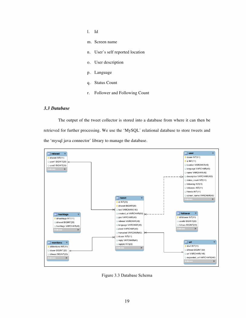
3.3 Database

The output of the tweet collector is stored into a database from where it can then be

retrieved for further processing. We use the ‘MySQL’ relational database to store tweets and

the ‘mysql java connector’ library to manage the database.

Figure 3.3 Database Schema

20

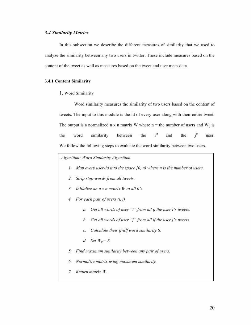
3.4 Similarity Metrics

In this subsection we describe the different measures of similarity that we used to

analyze the similarity between any two users in twitter. These include measures based on the

content of the tweet as well as measures based on the tweet and user meta-data.

3.4.1 Content Similarity

1. Word Similarity

Word similarity measures the similarity of two users based on the content of

tweets. The input to this module is the id of every user along with their entire tweet.

The output is a normalized n x n matrix W where n = the number of users and Wij is

the word similarity between the ith and the jth user.

We follow the following steps to evaluate the word similarity between two users.

Algorithm: Word Similarity Algorithm

1. Map every user-id into the space [0, n) where n is the number of users.

2. Strip stop-words from all tweets.

3. Initialize an n x n matrix W to all 0’s.

4. For each pair of users (i, j)

a. Get all words of user “i” from all if the user i’s tweets.

b. Get all words of user “j” from all if the user j’s tweets.

c. Calculate their tf-idf word similarity S.

d. Set Wij = S.

5. Find maximum similarity between any pair of users.

6. Normalize matrix using maximum similarity.

7. Return matrix W.

21

2. Hashtag Similarity

Figure 3.4 Hashtags in Twitter

The # symbol, called a hashtag, is used to mark keywords or topics in a

Tweet. Twitter users created it organically as a way to categorize messages.

3.4.2 Link Similarity

The input to this module is the id of every user along with all of their hashtags. The

output is a normalized n x n matrix H where n = the number of users and Hij is the hash-tag

Algorithm: Hashtag Similarity Algorithm


2. Initialize n x n matrix H to 0.

3. For each pair of user (i, j)

a. Calculate the total number of tweets ‘cnt’ of user i and user j which

have similar hash tags.

b. Set Hij = cnt.


5. Normalize matrix H using maximum similarity.

6. Return matrix H.

22

similarity between the ith and the jth user.

We follow the following steps to evaluate the hash-tag similarity between two users.

1. Retweet Similarity

Figure 3.5 Retweets in Twitter

When a user finds an interesting tweet written by another user and wants to

share it with her followers, she can retweet the tweet by copying the message,

typically preceding it with RT and addressing the original author with @. For

example, “RT @userA: my experience with #Ipad2 is great!” This practice has

become prevalent enough that Twitter now enables users to retweet easily with one-

click. A retweet is a relatively strong measure of similarity. Users generally retweet

another users tweet when they find the tweet interesting, they agree with the tweeters

opinion or to spread a message.

The input to the retweet based similarity analyzer is all the pairs of users who

have retweeted each other. The output is a normalized n x n matrix R whose element

Rij is the retweet similarity between two users i and j based on the number of times

they have retweeted each other and retweeted a common user. The pseudo-code of

the algorithm used to create the matrix R is given below.

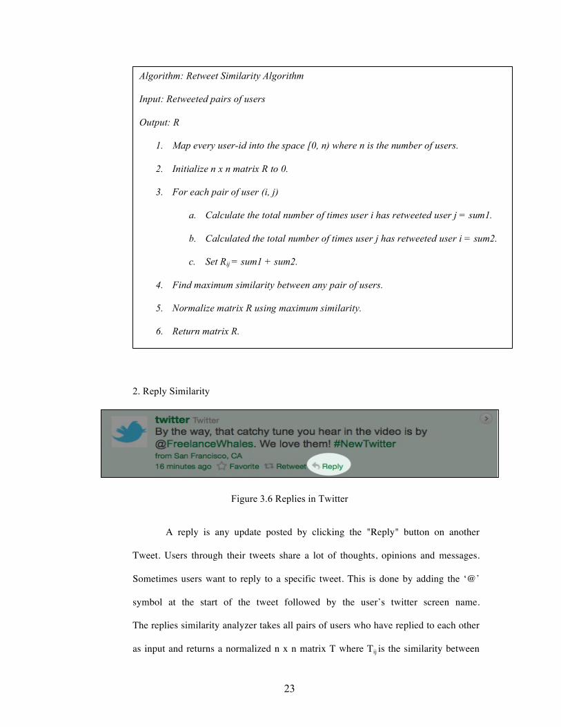
23

2. Reply Similarity

Figure 3.6 Replies in Twitter

A reply is any update posted by clicking the "Reply" button on another

Tweet. Users through their tweets share a lot of thoughts, opinions and messages.

Sometimes users want to reply to a specific tweet. This is done by adding the ‘@’

symbol at the start of the tweet followed by the user’s twitter screen name.

The replies similarity analyzer takes all pairs of users who have replied to each other

as input and returns a normalized n x n matrix T where Tij is the similarity between

Algorithm: Retweet Similarity Algorithm

Input: Retweeted pairs of users

Output: R


2. Initialize n x n matrix R to 0.


a. Calculate the total number of times user i has retweeted user j = sum1.

b. Calculated the total number of times user j has retweeted user i = sum2.

c. Set Rij = sum1 + sum2.


5. Normalize matrix R using maximum similarity.

6. Return matrix R.

24

any two users i and j based on the number of times they have replied to each other

and replied to any other common twitter user.

3. Mention Similarity

Figure 3.7 An Example of Mentions in Twitter

A mention is any Twitter update that contains @username anywhere in the

body of the Tweet. When one user wants to directly address another user, they do

so my putting the ‘@’ symbol in the body of the tweet followed by the users

twitter screen name. This is called ‘mentioning’ a user.

Algorithm: Reply Similarity Algorithm


2. Initialize n x n matrix T to 0.


a. Calculate the total number of times user i has replied to user j = sum1.

b. Calculated the total number of times user j has replied to user i = sum2.

c. Calculate the total number of times user i and user j have replied to a

common user = sum3

d. Set Tij = sum1 + sum2 + sum3.


5. Normalize matrix T using maximum similarity.

6. Return matrix T.

25

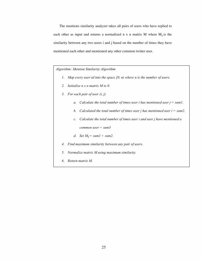
The mentions similarity analyzer takes all pairs of users who have replied to

each other as input and returns a normalized n x n matrix M where Mij is the

similarity between any two users i and j based on the number of times they have

mentioned each other and mentioned any other common twitter user.

Algorithm: Mention Similarity Algorithm


2. Initialize n x n matrix M to 0.


a. Calculate the total number of times user i has mentioned user j = sum1.

b. Calculated the total number of times user j has mentioned user i = sum2.

c. Calculate the total number of times user i and user j have mentioned a

common user = sum3

d. Set Mij = sum1 + sum2.


5. Normalize matrix M using maximum similarity.

6. Return matrix M.

26

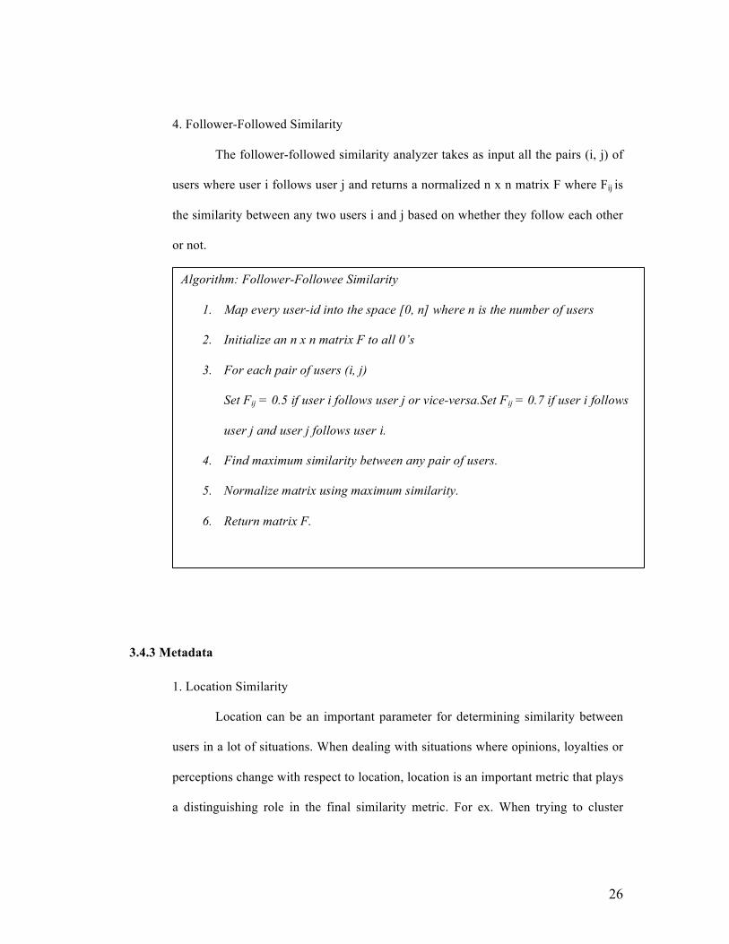
4. Follower-Followed Similarity

The follower-followed similarity analyzer takes as input all the pairs (i, j) of

users where user i follows user j and returns a normalized n x n matrix F where Fij is

the similarity between any two users i and j based on whether they follow each other

or not.

3.4.3 Metadata

1. Location Similarity

Location can be an important parameter for determining similarity between

users in a lot of situations. When dealing with situations where opinions, loyalties or

perceptions change with respect to location, location is an important metric that plays

a distinguishing role in the final similarity metric. For ex. When trying to cluster

Algorithm: Follower-Followee Similarity

1. Map every user-id into the space [0, n] where n is the number of users

2. Initialize an n x n matrix F to all 0’s

3. For each pair of users (i, j)

Set Fij = 0.5 if user i follows user j or vice-versa.Set Fij = 0.7 if user i follows

user j and user j follows user i.


5. Normalize matrix using maximum similarity.

6. Return matrix F.

27

twitterers of a worldwide sports event, their county plays an important role in

determining which team they support.

Figure 3.8 Twitter Users With Location (Figure Courtesy: www.sysomos.com)

A survey done by sysmos[] on over a billion tweets shows that the number of

users that share their location on their profile has increased from 44% in 2009 to 73%

in 2010 (http://www.sysomos.com). This location is the users self reported location

and is generally reported as the name of their city, state or country separated by ‘,’.

The input to the location similarity module is the list containing every user

with his self reported location. The output is a normalized n x n matrix L where every

element Lij is the similarity between user i and j based on their location.

As the user reported location is not in any specific format, we need to first

convert it into a standard format. We first split the users location on ‘,’. We then

check if any stripped element is a city by querying the ‘MySQL world database’. If it

28

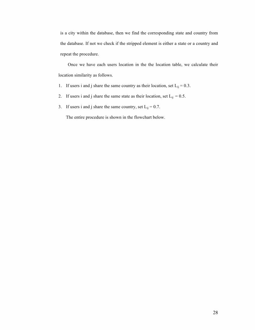
is a city within the database, then we find the corresponding state and country from

the database. If not we check if the stripped element is either a state or a country and

repeat the procedure.

Once we have each users location in the the location table, we calculate their

location similarity as follows.

1. If users i and j share the same country as their location, set Lij = 0.3.

2. If users i and j share the same state as their location, set Lij = 0.5.

3. If users i and j share the same country, set Lij = 0.7.

The entire procedure is shown in the flowchart below.

29

Figure 3.9 Flowchart - Location Similarity

3.5 Clusters

As the location similarity metric is not useful in all situations, it needs to be scaled

depending upon the kind of tweets being clustered.

3.5.1 N-Cuts

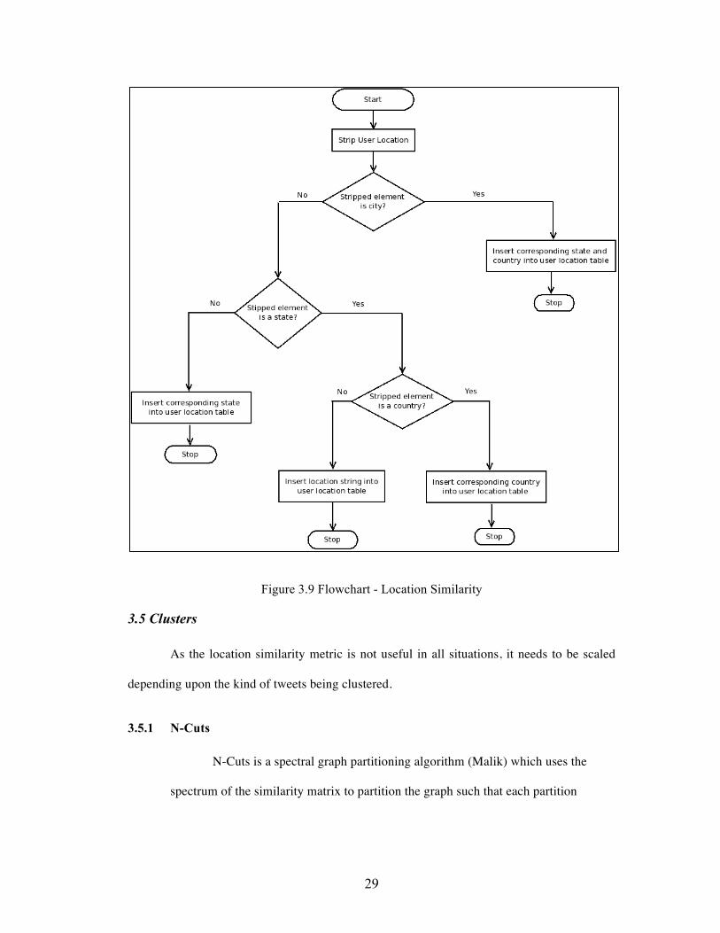
N-Cuts is a spectral graph partitioning algorithm (Malik) which uses the

spectrum of the similarity matrix to partition the graph such that each partition

30

minimizes the N-cut value. A detailed description of the algorithm is given in

Section.

1. Inputs

The similarity matrices calculated in the similarity metric step are added and

given as input to the N-cuts clustering module. The N-cut module uses this combined

similarity metric as its similarity matrix and uses its eigen-spectrum to find clusters.

2. Algorithm

3. Time Complexity

The main time constraint in the N-Cuts algorithm is in finding the

eigenvectors of the similarity matrix. In general calculation of the eigenvectors of

a n x n matrix takes O(n3) operations, which is relatively slow. But for most

practical purposes, we need only the leading eigen vectors of the normalized

Algorithm: N cuts

Input: W, R, P, M, L, no. of clusters = k

Output: k clusters

1. Initialize n x n similarity matrix S to all 0’s.

2. S = W + R + P + M + L

3. Compute diagonal matrix D of S; where, Di = Σ Si , 0 ≤ i ≤ n

4. Compute laplacian matrix L = D – W

5. Compute normalized laplacian L’ = D-1/2 L D-1/2

6. Compute the first k eigenvectors of L’ to form a k dimensional embedding of

the similarity graph in Euclidian Space.

7. Use k-means algorithm on the embedded clustering to generate the clusters.

31

laplacian. This can be done using the Lanczos method in relatively less time but

the performance declines if the graph cannot be easily well separated.

4. Disadvantages

a. The number of clusters k needs to be known beforehand.

b. The performance decreases when the number of clusters k increases.

3.5.2 Bottom-Up Agglomerative Clustering

Another important approach to clustering is hierarchical agglomerative bottom-up

clustering (Newman, Detecting Community Structure in Network). The idea behind this

technique is to develop a measure of similarity between every pair of users in the given

graph. Once one has such a measure then, starting with an empty network of n vertices and no

edges, one adds edges between pairs of vertices in order of decreasing similarity, starting

with the pair with strongest similarity. As the number of iterations increase the total number

of clusters goes on decreasing. At the start of the algorithm there are n components consisting

of a single vertex each, and at the very end there is just one component containing all

vertices. The components at each step along the way are perfectly nested inside the

components at the next step, so that the entire progress of the algorithm from start to finish

can be represented as a tree or dendrogram. Horizontal cuts through the tree at various

heights represent the communities found if the process is halted at the corresponding point. A

detailed description of the algorithm is given in section 2.1.1

32

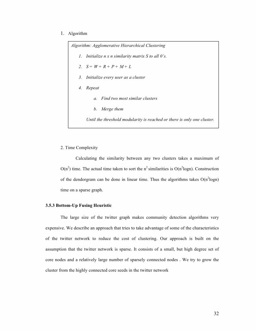
1. Algorithm

2. Time Complexity

Calculating the similarity between any two clusters takes a maximum of

O(n2) time. The actual time taken to sort the n2 similarities is O(n2logn). Construction

of the dendorgram can be done in linear time. Thus the algorithms takes O(n2logn)

time on a sparse graph.

3.5.3 Bottom-Up Fusing Heuristic

The large size of the twitter graph makes community detection algorithms very

expensive. We describe an approach that tries to take advantage of some of the characteristics

of the twitter network to reduce the cost of clustering. Our approach is built on the

assumption that the twitter network is sparse. It consists of a small, but high degree set of

core nodes and a relatively large number of sparsely connected nodes . We try to grow the

cluster from the highly connected core seeds in the twitter network

Algorithm: Agglomerative Hierarchical Clustering

1. Initialize n x n similarity matrix S to all 0’s.

2. S = W + R + P + M + L

3. Initialize every user as a cluster

4. Repeat

a. Find two most similar clusters

b. Merge them

Until the threshold modularity is reached or there is only one cluster.

33

1. Twitter Network Statistics

a. It has been shown by Java et al. that the cumulative follower degree distribution for

Twitter follows a power law with an exponent of about -2.4 (Akshaya Java). In other

words, a very little number of twitter users hold a very high proportion of incoming

links.

b. A small hard-core group (2.2%) have accounted for 58.3% of all tweets, while

22.5% have accounted for about 90% of all activity (http://www.sysomos.com).

Figure 3.10 Tweets Posted (Figure Courtesy: www.sysomos.com)

c. On average, Twitter users have five degrees of separation between each other -

meaning nearly everyone within Twitter is only five steps away

(http://www.sysomos.com). Of all friendship distances, five steps is the most

common (41%), while a friendship distance of four steps is the second-most common

(37%).on average, a Twitter user will encounter 83% of all other Twitter users by

34

visiting everyone's friends up to a distance of five steps. Here is a pie chart that

shows the different Twitter friendship distances:

Figure 3.11 Degree of Separation in Twitter Graph (Figure Courtesy: www.sysomos.com)

2. Method

Figure 3.12 Determination of Seeds of the Graph

35

i. Step 1: Find out the seeds of the graph.

We find the seeds by finding out the users who have the most

a. Followers

b. Have been retweeted the most

c. Have been mentioned the most

d. Have been replied to the most

We consider these seeds as the initial clusters and will find

communities based on the connections emerging from these seeds.

Figure 3.13 Finding The Immediate Neighborhood of Each Seed

ii. Step 2: For each of the clusters do the following

a. Find the 1-neighborhood ie the immediate neighbors of

each of the users in the cluster. We define immediate

neighbors as the users that each of the users in the current

cluster

36

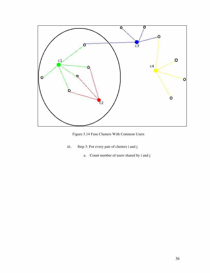
Figure 3.14 Fuse Clusters With Common Users

iii. Step 3: For every pair of clusters i and j

a. Count number of users shared by i and j

37

Figure 3.15 Resolve Users That Belong to More Than One Community

Figure 3.16 Repeat Until Terminal Condition is Reached

38

iv. Step 4: For every user that is present in more than one cluster

a. Allocate it to the cluster to which it shares the maximum

links to

v. Step 5: Calculate the modularity value of the clustering

vi. Step 6: Repeat until

a. No more clusters can be merged

b. All users have been assigned to a cluster

c. The desired number of clusters has been reached

d. The maximum modularity value has been reached

vii. Step 7: If there are users that do not belong to any cluster, allocate

them to the cluster they are most similar according to word-

similarity, hashtag-similarity or location similarity and other

metrics.

39

Chapter 4: Results

4.1 Datasets

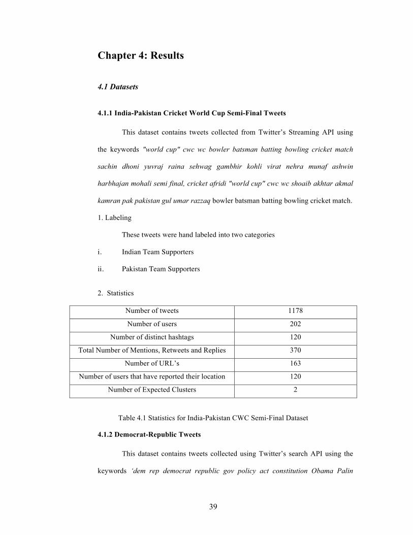
4.1.1 India-Pakistan Cricket World Cup Semi-Final Tweets

This dataset contains tweets collected from Twitter’s Streaming API using

the keywords "world cup" cwc wc bowler batsman batting bowling cricket match

sachin dhoni yuvraj raina sehwag gambhir kohli virat nehra munaf ashwin

harbhajan mohali semi final, cricket afridi "world cup" cwc wc shoaib akhtar akmal

kamran pak pakistan gul umar razzaq bowler batsman batting bowling cricket match.

1. Labeling

These tweets were hand labeled into two categories

i. Indian Team Supporters

ii. Pakistan Team Supporters

2. Statistics

Number of tweets 1178

Number of users 202

Number of distinct hashtags 120

Total Number of Mentions, Retweets and Replies 370

Number of URL’s 163

Number of users that have reported their location 120

Number of Expected Clusters 2

Table 4.1 Statistics for India-Pakistan CWC Semi-Final Dataset

4.1.2 Democrat-Republic Tweets

This dataset contains tweets collected using Twitter’s search API using the

keywords ‘dem rep democrat republic gov policy act constitution Obama Palin

40

president "white house" pres prez demc clinton hillary mayor senator biden jobs

health economic politic sarah "tea party" conservative’’.

1. Labeling

The data was hand labeled into the following two categories

i. Democrat

ii. Republic

2. Statistics


Number of users 535




Number of users that have reported their location 264


Table 4.2 Statistics For Democrat-Republic Dataset

4.1.3 Indian Premier League Tweets

The IPL is a domestic T20 cricket tournament played in India in which

players from all over the world participate. We collected tweets of five different

teams using the names of the teams and their players as search keywords.

1. Labeling

We used Amazon Mechanical Turk for labeling the tweets[]. Each turker was

presented with all the tweets of one twitter user and was asked to identify the team he

supports. We used time filters to remove spam. Each user was labeled into one of the

following five categories:

i. Mumbai Indians

ii. Sahara Pune Warriors

41

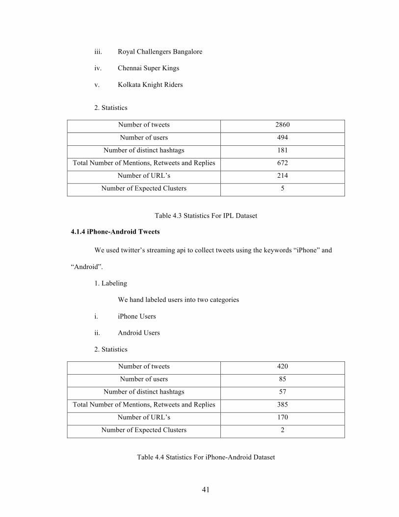
iii. Royal Challengers Bangalore

iv. Chennai Super Kings

v. Kolkata Knight Riders

2. Statistics


Number of users 494





Table 4.3 Statistics For IPL Dataset

4.1.4 iPhone-Android Tweets

We used twitter’s streaming api to collect tweets using the keywords “iPhone” and

“Android”.

1. Labeling

We hand labeled users into two categories

i. iPhone Users

ii. Android Users

2. Statistics


Number of users 85





Table 4.4 Statistics For iPhone-Android Dataset

42

4.1.5 Tweets Pertaining to Different Universities in Maryland

We identified official accounts of the following universities in Twitter:

i. UMBC

ii. UMD

iii. JHU

iv. Towson

1. Labeling

The users were hand labeled to identify which universities they belong to.

2. Statistics


Number of users 100





Table 4.5 Statistics for Universities in Maryland Dataset

4.2 Definitions

4.2.1 Rand Index

We used the rand index to validate the clusters. The Rand index or Rand measure

in statistics, and in particular in data clustering, is a measure of the similarity between two

data clustering.

RandIndex = TruePositive+TrueNegativeTruePositive+FalsePositive+TrueNegative+FalseNegative

43

4.2.2 Modularity Score

Newman and Girvan (Newman, Modularity and Community Structure in Networks)

proposed that the divisions the algorithm generates be evaluated using a measure they call

modularity, which is a numerical index of how good a particular division is. For a division

with g groups, we define a g × g matrix e whose component eij is the fraction of edges in the

original network that connect vertices of group i to those of group j. Then the modularity is

defined to be

! = !!!!

− !!" !!" = !! ! − | !! |!"#

where x indicates the sum of all elements of x. Physically, Q is the fraction of all edges that

lie within communities minus the expected value of the same quantity in a graph in which the

vertices have the same degrees but edges are placed at random without regard for the

communities. A value of Q = 0 indicates that the community structure is no stronger than

would be expected by random chance and values other than zero represent deviations from

randomness. Local peaks in the modularity during the progress of the community structure

algorithm indicate particularly good divisions of the network.

4.3 Cluster Validation

4.3.1 N-Cuts

1. Content Similarity

To evaluate the effectiveness of the content similarity metrics, we clustered users

using the word and hash-tag similarity metrics and calculated the rand-index.

44

Figure 4.1 N-Cuts: Content Similarity

N-Cuts

India vs. Pakistan World Cup Semifinal 0.52

Democrat – Republic 0.56

Indian Premier League 0.52

iPhone – Android 0.73

Universities 0.61

Table 4.6 N-Cuts: Content Similarity

i. Analysis of Content Similarity

Word Similarity has traditionally been an important similarity metric

for clustering of social-networks. But as we can see in the results above the

word similarity similarity metric does not do very well for the india-pakistan

and the dem-republican dataset. It performs better on the iphone-android

dataset.

0 0.1 0.2 0.3 0.4 0.5 0.6 0.7 0.8

Content Similarity

Content Similarity

45

Our intuition is that when we are clustering tweets on a single event

and are trying to cluster users based on their perceptions and opinions, word

similarity does not play a very important role in distinguishing users of

different communities. This is because the users belonging to different

communities are tweeting about the same thing but have different opinions

about them.

a) India-Pakistan CWC Semi-Final

Label Words

India watch, tendulkar, indian, sachin, lagta, teams, world,lose, #cwc2011, bowling, one,

india's, media, @bhogleharsha:, kii, mohali, win, sri, it's, news, @skipperafridi,

surprised, #cricket, cricket, minister, india, @espncricinfo, time, malik, pak, cup,

final, mohali, team, play, india-pakistan, @jhunjhunwala, south, rehman, dhoni,

india's, match, pm, batti, #wc11, suspect, pakistan, yuvraj, wc, vs, lanka, se, rt,

munaf, contest, batting, aur

Pakistan fakmal, country, boys, indian, world, voice., #cwc2011, media, pakistani, vich, sri,

zealand, it's, @skipperafridi, #cricket, afridi, #worldcup, hai, pak, lobby, final,

team, play, rehman, people, match, gali, icc, pm, earth, ki, ko, wa, vs, rt, shoaib,

shit, owes, shor, ay, *gali, singing, #pakistan, mohali, win, via, cricket, minister,

india, hour, malik, day, cup, semi, shahid, match, doing, fucking, afridi's, hotel,

pakistan, top, batting

Table 4.7 Most Common Words

Label Words

India mohali, pakistan, wc11, cricket, worldcup, cwc2011, mohali30mar, cwc, fb, cwc11

Pakistan mohali, afridi, pakistan, wc11, cricket, worldcup, pakcricket, cwc2011, tgme,

lahore, india, cwc11, bringshoaibback

Table 4.8 Most Common Hashtags

46

b) iPhone-Android

Label Words

Iphone Mac, verizon, releases, ipad, released, location, iphone, apple, @iphone_news,

ipod, htt, ios, white, jailbreak, rt, iphone, tracking, touch

Android video, motorola, live, next-generation, updated, @androidcentral, #android, update,

xperia, ericsson, @androidandme, @androiddev, @connectandroid, sony, tablet,

pro, android, launches, mini, phone, samsung, post, t-mobile, maps, #io2011,

@phandroid, #android, @androidpolice, galaxy, io, sprint, htc, rt, android, via,

xprt, titanium, google, version, app, mini, market

Table 4.9 Most Common Words

Label Words

Iphone app, nowplaying, ipod, ios4, download, iphone, itunes

Android htc, androidjp, android, iphone, io2011

Table 4.10 Most Common Hashtags

We can see in the tables above that in the India-Pakistan World Cup

semifinal dataset, users from both the communities are frequently using the same

words and hash-tags. Thus the word-similarity metric doesn’t perform very well on

this dataset.

On the other hand the words and hash-tags used in the the two communities

in the iphone and android dataset are considerably different. Thus word-similarity

performs better on this dataset.

2. Link Similarity

To evaluate the effectiveness of link similarity metrics, we clustered tweets

using the retweet, mentions and replies similarity metric and calculated the rand

index.

47

Figure 4.2 N-Cuts: Link Similarity

N-Cuts

India vs. Pakistan World Cup Semifinal 0.77

Democrat – Republic 0.75

Indian Premier League 0.73

iPhone – Android 0.85

Universities 0.72

Table 4.11 N-Cuts: Link Similarity

3. Content, Link and Metadata Similarity

To evaluate the overall effectiveness of the similarity metric, we added all

the similarity metrics together and then calculated the rand index.

0.65 0.7 0.75 0.8 0.85 0.9

Link Similarity

Link Similarity

48

Figure 4.3 N-Cuts: Content, Link & Metadata Similarity

Data-Set Rand Index #Clusters

India vs. Pakistan World Cup Semifinal 0.74 2

Democrat – Republic 0.73 2

Indian Premier League 0.72 5

iPhone – Android 0.79 2

Universities 0.69 4

Table 4.12 N-Cuts: Content, Link & Metadata Similarity

4.3.2 Bottom-Up Agglomerative Hierarchical

The rand-indices as calculated by the bottom-up fusing heuristic are given in

the table below.

0.64 0.66 0.68 0.7 0.72 0.74 0.76 0.78 0.8

Rand Index

Rand Index

49

Figure 4.4 Bottom-Up Agglomerative Hierarchical: India-Pakistan CWC Semi-Final

Number of Clusters Modularity Index Rand Index

30 0.193684267 0.753265932

29 0.1862532 0.760045793

28 0.185668785 0.766079085

27 0.196529922 0.771582294

26 0.191566887 0.762507058

25 0.191562391 0.760810196

24 0.191548905 0.761029412

23 0.191548905 0.763882353

22 0.19427318 0.759694619

21 0.271438497 0.756663801

20 0.270427008 0.760040671

19 0.273155779 0.754286435

18 0.272557877 0.753491352

17 0.283526906 0.749484802

16 0.283081851 0.764935941

15 0.288809122 0.775456558

14 0.286516415 0.767696173

-‐0.4

-‐0.2

0

0.2

0.4

0.6

0.8

1

1.2

201

189

177

165

153

141

129

117

105 93

81

69

57

45

33

21 9

Modularity Score

Rand Index

50

13 0.288418013 0.766876556

12 0.278280652 0.777952261

11 0.25360933 0.748852236

10 0.264902036 0.738464187

9 0.005507003 0.580084547

8 -0.004931555 0.603417944

7 -0.023084399 0.602409639

6 -0.026806676 0.622111526

5 -0.166580859 0.624042581

4 -0.284875532 0.505705157

3 -0.333179721 0.536189181

Table 4.13 Bottom-Up Agglomerative Hierarchical: India-Pakistan CWC Semi-Final

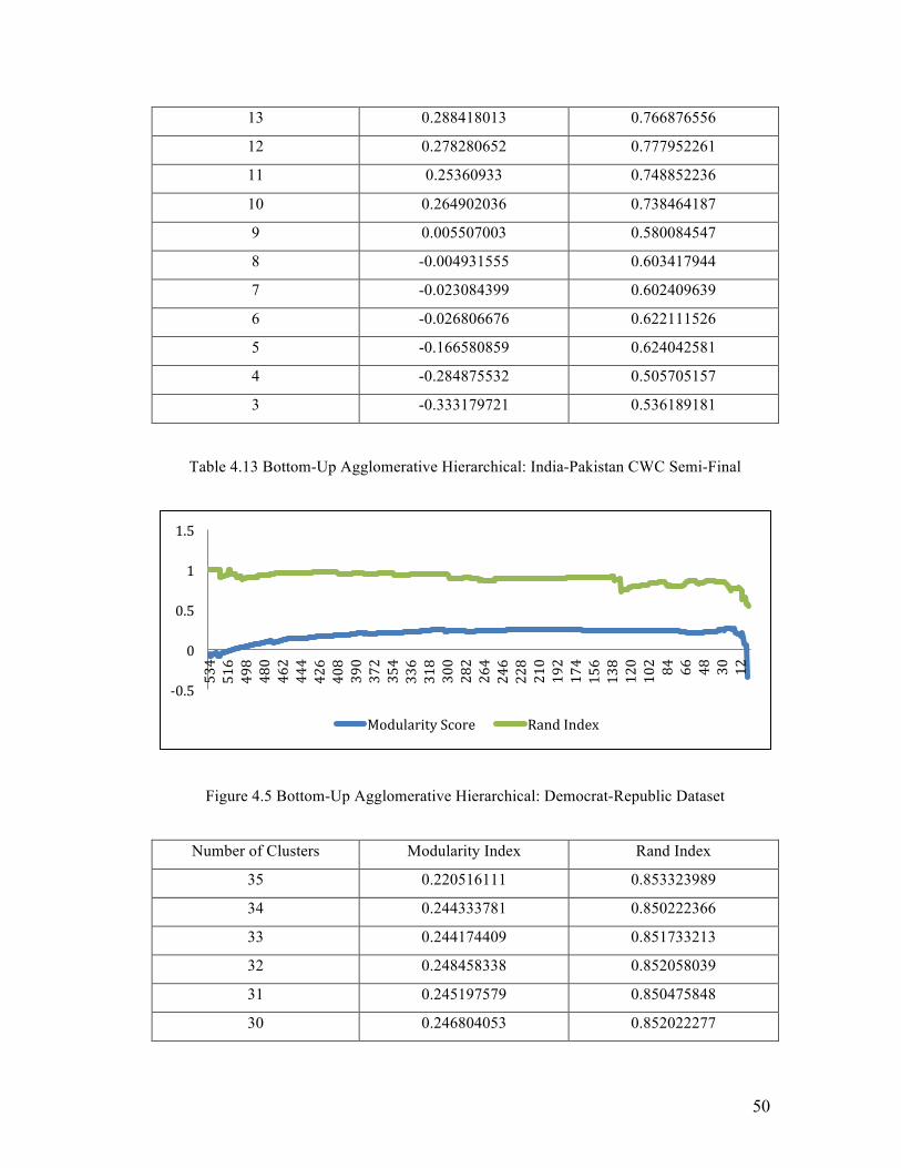
Figure 4.5 Bottom-Up Agglomerative Hierarchical: Democrat-Republic Dataset


35 0.220516111 0.853323989

34 0.244333781 0.850222366

33 0.244174409 0.851733213

32 0.248458338 0.852058039

31 0.245197579 0.850475848

30 0.246804053 0.852022277

-‐0.5

0

0.5

1

1.5

534

516

498

480

462

444

426

408

390

372

354

336

318

300

282

264

246

228

210

192

174

156

138

120

102 84

66

48

30

12

Modularity Score Rand Index

51

29 0.251338728 0.848855247

28 0.250344244 0.850208044

27 0.245148705 0.844659044

26 0.266895596 0.835639308

25 0.266555602 0.824009636

24 0.266176296 0.811333536

23 0.265761927 0.794067271

22 0.264173516 0.780995713

21 0.260858571 0.762481896

20 0.260399578 0.740997308

19 0.256986885 0.763901043

18 0.255609907 0.764907916

17 0.265168 0.768474621

16 0.216914296 0.770015111

15 0.21093677 0.766163561

14 0.205731668 0.770547836

13 0.201570987 0.777542268

12 0.19983489 0.769163748

11 0.174054816 0.746914789

10 0.16954564 0.734555105

9 0.211428699 0.633194505

8 0.161145654 0.643784559

7 0.08134897 0.642496885

6 0.05363199 0.651308039

5 0.054812408 0.572019665

4 -0.350368469 0.565355734

3 -0.3601243588 0.550960667

Table 4.14 Bottom-Up Agglomerative Hierarchical: Democrat-Republic Dataset

52

Figure 4.6 Bottom-Up Agglomerative Hierarchical: IPL Dataset


25 0.401420593 0.806781323

24 0.404592551 0.806195882

23 0.404577265 0.805138016

22 0.404470259 0.803062072

21 0.404449877 0.801469407

20 0.404449877 0.799828844

19 0.404437138 0.797760238

18 0.403479182 0.792636892

17 0.418438328 0.792733418

16 0.417707122 0.790576609

15 0.417645976 0.786875541

14 0.334697406 0.780359551

13 0.324370077 0.740875352

12 0.33450123 0.778405565

11 0.329291066 0.756265502

10 0.329219729 0.754643875

9 0.329184061 0.753715333

-‐0.2

0

0.2

0.4

0.6

0.8

1

1.2

293

275

257

239

221

203

185

167

149

131

113 95

77

59

41

23 5

Modularity Score

Rand Index

53

8 0.32063634 0.745685702

7 0.320279653 0.716176658

6 0.064951185 0.6219706

5 0.058541031 0.59570833

4 0.05925313 0.58552752

Table 4.15 Bottom-Up Agglomerative Hierarchical: IPL

4.3.3 Bottom-Up Fusing Heuristic

Figure 4.7 Bottom-Up Fusing Heuristic: India-Pakistan CWC Semi-Final

Number of Clusters Modularity Index Rand Index 52 0.751508814 0.83296973 51 0.764851467 0.838975051 50 0.779848464 0.834238051 26 0.808237566 0.745642505 24 0.830431868 0.75257061 13 0.694739597 0.716386812 12 0.687731106 0.725804704 7 0.588722143 0.821094609

-‐0.4

-‐0.2

0

0.2

0.4

0.6

0.8

1

114 84 74 68 62 58 56 54 52 50 24 12 6 3

Modularity

Rand Index

54

6 0.462259127 0.745998921 4 0.010933069 0.761408767 3 -0.21173821 0.752402023 2 -0.3 0.63

Table 4.16 Bottom-Up Fusing Heuristic: India-Pakistan CWC Semi-Final

Figure 4.8 Bottom-Up Fusing Heuristic: Democrat-Republic Dataset

Number of Clusters Modularity Index Rand Index 49 0.878719539 0.919784929 28 0.88591807 0.818173982 17 0.865974764 0.817427471 10 0.872271885 0.801186345 6 0.182896795 0.659609675 4 0.381281396 0.554015182 3 -0.40831945 0.546800635

Table 4.17 Bottom-Up Fusing Heuristic: Democrat-Republic Dataset

-‐0.6

-‐0.4

-‐0.2

0

0.2

0.4

0.6

0.8

1

1.2

154 126 113 109 106 103 102 101 100 99 98 97 96 95 94 93 49 28 17 10 6 4 3

Modularity Rand Index

55

Figure 4.9 Bottom-Up Fusing Heuristic: IPL Dataset


50 0.8319124 0.92090668 26 0.820379985 0.865153153 24 0.848875362 0.849638639 13 0.789191625 0.851922293 7 0.610829586 0.779544304 4 0.102735686 0.671259548 3 -0.7333449 0.460643832

Table 4.18 Bottom-Up Fusing Heuristic: IPL Dataset

-‐1 -‐0.8 -‐0.6 -‐0.4 -‐0.2 0

0.2 0.4 0.6 0.8 1

1.2

126 103 94 88 83 78 74 70 67 64 61 59 57 55 53 51 50 26 24 13 7 4 3

Modularity Score Rand Index

56

Chapter 5: Conclusion and Future Work

5.1 Conclusion

We proposed and described an approach to cluster users in twitter based on their

content, link and meta-data similarity. We analyzed the performance of two standard

clustering algorithms for clustering users in twitter. We also analyzed the effectiveness of

various similarity measures in different types of situations. From our results we conclude that

link similarity is a better indicator of similarity between users as compared to content

similarity. We calculated link similarity by analyzing connections between users based on

retweets, mentions, replies and follower-following relationships. Content Similarity is useful

in domains where the clusters to be found are based on “” as compared to clusters based on

affiliations and opinions.

Detecting communities over the extremely large social graph of twitter is

challenging. One way to do this is to analyze the core of the social graph and user this core to

grow communities. If we chose the core carefully, we can find a good approximation of the

community structure of the entire graph. Given the power law distribution of twitter we

introduced a heuristic that takes advantage of the characteristics of the twitter network to

cluster users quickly and efficiently.

57

5.2 Future Work

1. Clustering to find groups is one aspect of community detection, identifying and

characterizing them is another. Our work focuses only on detecting communities.

Identifying communities based on their link structure and the content and meta-data

of consisting users is an interesting problem that can be studied further.

2. Sentiment can be used in analyzing and detecting communities. Sentiment

associated with @mentions and hash-tags can be used as a measure of similarity

between two users to detect communities

3. In our work, we do not weigh similarity metrics before adding them. Determining

optimal weights for each similarity metric before combining them can be an

important step to increase accuracy.

58

Bibliography

• Capocci, V. D. Detecting Communities in Large Networks.

• Yee Whye Teh, H. D. Bayesian Agglomerative Clustering with Coalescents.

• Akshay Java, A. J. Detecting Communities via Simultaneous Clustering of Graphs

and Folksonomies.

• Akshay Java, T. F. Approximating the Community Structure of the Long Tail.

• Akshaya Java, T. F. Why We Twitter: Understanding Microblogging Usage and

Communities.

• Amanda Lee Hughes, L. P. Twitter Adoption and Use in Mass Convergence and

Emergency Events.

• Bernard J. Jansen and Mimi Zhang, K. S. Twitter Power: Tweets as Electronic Word

of Mouth.

• Boyd D., G. S. Tweet, Tweet, Retweet: Conversational Aspects of Retwitting on

Twitter.

• Bongwon Suh, L. H. Want to be Retweet? Large Scale Analytics on Factors

Impacting Retweet in Twitter Network.

• Clauset, A. Finding Local Community Structure in Network.

• D., Z. Science of Retweets.

• Dhillon, I. S. Co-clustering documents and words using Bipartite Spectral Graph

Partitioning.

59

• Gernot Tscherten, C. L. Community Core Detection in Twitter - a "Bottom-Up"

Heuristic.

• Hughes A. L., P. L. "Site-Seeing" in Disaster: An Examination of On-line Social

Convergence.

• Haewoon Kwak, C. L. What is Twitter, a Social Network or a News Media.

• http://www.sysomos.com. (n.d.). Retrieved from

http://www.sysomos.com/company/reports-and-whitepapers/:

• Java, A. A Framework for Modeling Influence, Opinions and Structure in Social

Media.

• Java, A. Mining Social Media Communities and Content (Chapter IV). In A. Java.

• Kale Anubhav, e. a. Modeling Trust and Influence in the Blogosphere Using Link

Polarity.

• Luxburg, U. v. A Tutorial on Spectral Clustering.

• Lei Tang, X. W. Community Detection in Multi-Dimensional Networks.

• Newman, M. E. Detecting Community Structure in Network.

• Newman, M. E. Modularity and Community Structure in Networks.

• Nina Mishra, R. S. Clustering Social Networks.

• M. Girvan, M. E. Community Structure in Social and Biological Networks.

• MacQueen, J. B. Some Methods for Classification and Analysis of Multivariate

Observations.

• Malik, J. S. Normalized Cuts and Image Segmentation.

• Manning, C. D., Raghavan, P., & and Schutze, H. Introduction to Information

Retrieval.

• Meeyoung Cha, H. H. Measuring User Influence in Twitter: The Million Follower

Fallacy.

60

• Michael J. Welch, D. H. Topical Semantics of Twitter Links.

• Sutton J., P. L. Back-Channels in the Front Lines: Emerging Use of Social Media.

• Stelter B., C. N. Citizen Journalists Provided Glimpses of Mumbai Attacks, The New

York Times.

• Tim Finin, e. a. The Information ecology of social media and online communities.

approval sheet - umbc ebiquity research groupebiquity.umbc.edu/get/a/publication/588.pdf ·...

Documents