applied statistics and experimental...
TRANSCRIPT

Applied Statistics and Experimental DesignObservational Studies & Controlled Experiments
Fritz Scholz
Fall Quarter 2008
Census and Samples→ Induction
Statistics originally served to describe matters of the state (status of state)
by capturing numerically various aspects of full populations.
Today this is called a census, from Latin censere (to count or estimate).
−→ historical census of Emperor Augustus.
Much of statistics as a discipline focusses on samples, i.e., part of the total.
The goal is to draw conclusions about the whole population (generalize).
This process is referred to as induction, from Latin inducere (to lead to).
Its validity or compelling force depends crucially on the process of sampling.
Sample←− example←− Latin exemplum←− eximere to take out.
1

Brass Grain Probes–Stick Probe
Stichprobe
German
for Sample
2

Chicago Board of Trade (CBOT)
3
Sampling Issues and Problems
Obviously the grain sample was not random, there was a systematic aspect.
The idea was to represent all parts of the whole shipment.
However, you probably could still escape scrutiny in the bottom 2′′ layer,
or if layers were carefully arranged (based on known probe characteristics).
Long ago a pharmacist was accused of Medicare fraud, supposedly charging
for nonexistent transactions, i.e., making them up.
To obtain evidence the prosecutors had examined every kth transaction in his file.
Prior to computers this was a convenient process, but with problems.
It might be considered a random sample, if the transaction files had been shuffled
randomly a priori, but that was not done.
Assuming that the order is random does not make it a random sample.
My role was to point out the weaknesses in the prosecution’s process.
4
Observational Studies
In an observational study we are just passive observers.
We do not tinker with any aspect of what is observed, except that we do observe.
We observe by obtaining counts/measurements on several variables.
This could be done on a full population or on some kind of sample.
Sampling could be random or not (a possible non-passive aspect of observing).
It is not clear which variables have an effect on which other variables
if we observe any patterns or correlations. =⇒ The causality issue.
There may be unmeasured factors that affect several of the measured variables,
their resultant correlation suggesting causality between them.
The next four slides (inspired by Box, Hunter & Hunter) are a humorous attempt
illustrate the latter point.
5
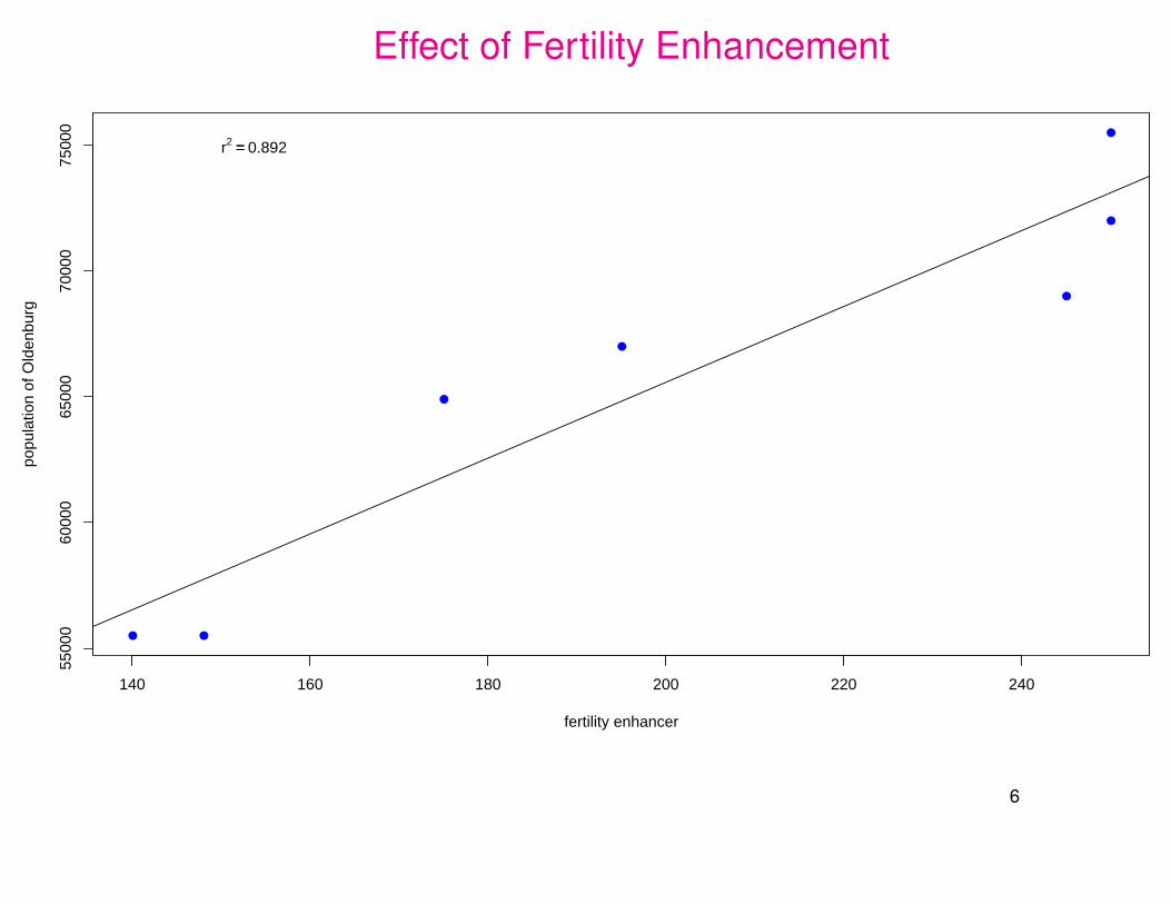
Effect of Fertility Enhancement
● ●
●
●
●
●
●
140 160 180 200 220 240
5500
060
000
6500
070
000
7500
0
fertility enhancer
popu
latio
n of
Old
enbu
rg
r2 == 0.892
6
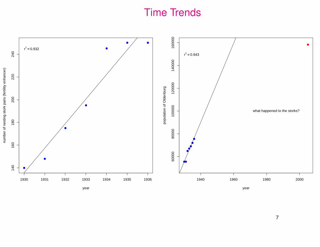
Time Trends
●
●
●
●
●
● ●
1930 1931 1932 1933 1934 1935 1936
140
160
180
200
220
240
year
num
ber
of n
estin
g st
ork
pairs
(fe
rtili
ty e
nhan
cer)
r2 == 0.932
●●
●●
●
●
●
1940 1960 1980 2000
6000
080
000
1000
0012
0000
1400
0016
0000
year
popu
latio
n of
Old
enbu
rg
r2 == 0.943
●
what happened to the storks?
7

Data Source
DALLINGA & SCHOENMAKERS WHITE STORK DECREASE 169
and 1984 the number of eastern storks in West Germany has decreased by about 74%. (The international census data of 1934 are extrapolated to 1928, because, as will be shown later, the numbers in that year seem to be more comparable with those after the 1950s with respect to the conditions in the wintering area.)
In Denmark, situated to the north of West Germany, the downward trend was still greater; in the period 1928-1984 num- bers decreased by about 96%. In the coun- tries situated to the east of West Germany, however, where 'the same fluctuations in numbers occurred, no such downward trend can be discerned, certainly not since the end of the 1920s (see graph 5 Milicz in Figure 2). It is true, regionally numbers decreased, but these decreases seem to have been amply compensated for by in- creases in other regions, partly by expan-
I sion, partly by growing densities (see graph 6 Oberlausiu in Figure 2). It is esti- 1 - mated that in East Germany numbers have
? - increased in this way by 7% since 1928. In M the northern part of the Soviet Union this 5 .- P
percentage is higher still, in that the breed- P .- ing range expanded to the east and north- x east, a process which has been in progress
since at least the first half of the 19th cen- Figure 2. Changes in number of pairs of storks in the census regions shown in Figure 1, given as per- centages of the numbers in base-line census years, 1934 unless otherwise given in Table 1. The graphs 1-11 refer to regions with predominantly eastern storks, graph If refers to a region with, at first, a mixing of eastern and western storks (since the 1950s predominantly eastern storks), and the graphs 13 and 14 refer to regions with predominantly west- ern storks. Broken lines connect irregular censuses. The two periods for Oberlausitz (graph 6) are based on partly different districts. The Dutch data (graph If) for the period 1931-1943 are extrapolations with respect to the complete censuses of 1934 and 1939.
except the years 1937 and 1938. In con- trast, the 1940s and early 1950s were very poor, particularly 1941 (with a decrease in Oldenburg of 28%) and 1949 (32% de- crease). From 1954 to 1962 numbers in- creased, reaching a maximum in 1962. After that numbers decreased fairly stead- ily. However, 1974 was very favorable, with an increase of 18%.
Over a longer term, a clear downward trend in the level of the fluctuations can be discerned, probably dating to the 19th century. It is estimated, that between 1928
tury. In south-east Europe, regional cen-
suses in the Balkan States suggest that numbers have decreased in the past dec- ades by a few tens of percents. In Hun- gary, however, an initially sharp decrease changed into an increase of 19% in the period 1974- 1984.
Among western storks, numbers in north-western Europe (see graphs 13 and 14 in Figure 2) decreased in the second half of the 19th and in the early 20th cen- tury. Whether there have been temporary increases in this period is not known. In the 1930s and again in the course of the 1940s numbers stabilized and regionally rose, reaching a maximum in 1948. After sharp decreases in 1949 and 1950, a clear increase followed in 1955-1960. In 1961, however, numbers decreased again by about 24%. This was the first year of a 15- year period with almost continuously de- creasing numbers.
The census data of the southern parts of the breeding range of the western storks are insignificant to indicate long term
Regional Decrease in the number of White Storks
(Ciconia c. ciconia) in Relation to Food Resources,
J.H. Dalinga and S. Schoenmakers (1987)
Colonial Waterbirds, Vol. 10, No. 2, 167-177.
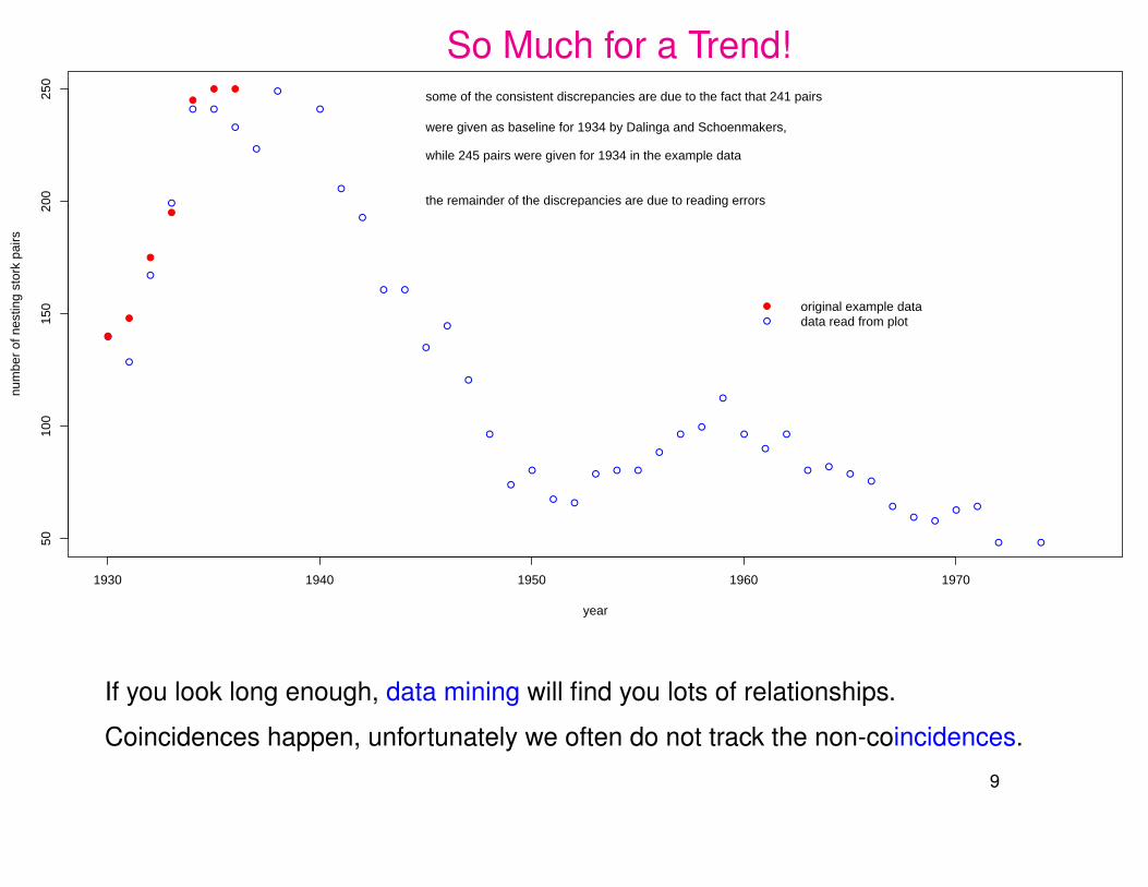
Plot 11 represents the nesting stork pair population
in Oldenburg.
Note the interesting superposition of many time
lines of % of baseline values in 1934.
(241 for Oldenburg in 1934)
8
So Much for a Trend!
●
●
●
●
● ●
●
●
●
●
●
●
●
● ●
●
●
●
●
●
●
● ●
● ● ●
●
●●
●
●
●
●
● ●●
●
●
● ●
● ●
●
●
●
●●
1930 1940 1950 1960 1970
5010
015
020
025
0
year
num
ber
of n
estin
g st
ork
pairs
●
●
●
●
●
● ●
●
●
original example datadata read from plot
some of the consistent discrepancies are due to the fact that 241 pairs
were given as baseline for 1934 by Dalinga and Schoenmakers,
while 245 pairs were given for 1934 in the example data
the remainder of the discrepancies are due to reading errors
If you look long enough, data mining will find you lots of relationships.
Coincidences happen, unfortunately we often do not track the non-coincidences.
9
Controlled Experiments
In a controlled experiment we control the values of certain input variables.
We are no longer passive observers. We experiment (Latin experiri: from trying).
We observe the values of the other, not directly controlled variables and examine
whether any patterns, reactions or relationships emerge as a result of the controlled
input variables.
These other variables are called response variables. It is hoped that they will show
changed and ≈ reproducible values in response to the controlled input levels.
−→ cause and effect. The case of the moving pencil.
We need to avoid any conscious or subconscious biases in the inputs.
Example: Assign healthier patients to a new treatment.
Such biases may contribute to any observed treatment effect (→ confounding).
We don’t know how much of the effect is due to bias and/or treatment.10
Hormone Replacement Therapy for Post-Menopausal Women
US Food and Drug Administration-approved indications for hormone therapy
include relief from menopausal symptoms and osteoporosis.
Approximately 38% of postmenopausal women in the US use
hormone replacement therapy (as reported in 1999).
In 2000, 46 million prescriptions for Premarin, more than $1 billion in sales.
22.3 million prescriptions for Prempro, possibly another $500 million/year.
Long-term use has been in “vogue” to prevent a range of chronic conditions,
especially coronary heart disease (CHD).
The above 38% certainly reflect this long-term usage.
11

Effect of Estrogen Treatment on Post-Menopausal Women?
Population: Healthy post-menopausal women in the U.S.
Potential “input” or causal variables:
estrogen treatment (yes/no)
demographic variables (age, race, family history, ...)
unmeasured variables (education level, diet, level of fitness exercising, . . .).
These other variables may be used to correct for their impact on the response.
Possible output variables (responses or “causal consequences”):
coronary heart disease (CHD, primary), invasive breast cancer (secondary),
stroke, pulmonary embolism (PE), endometrial cancer, colorectal cancer,
hip fracture, and others.
Question: How does estrogen treatment affect health outcomes?
12
Results of Prior Observational Studies
In earlier observational studies, variables of interest were measured
for each subject in available samples (possibly random).
In that sense they may be representative of the general population as is.
The use of estrogen was determined by each woman prior to the study.
Findings: good health and low rates of CHD are more prevalent in the estrogen
portion of the sample.
In fact, these studies suggested a 40%-50% reduction in CHD risk among users
of estrogen alone or, less frequently, of combined estrogen and progestin.
Estrogen alone was the dominant hormone until the increased risk of endometrial
cancer led to the addition of progestins for women with intact uterus. There were
also indications of increased breast cancer risk related to duration of therapy.
13

Sources: WHI Randomized Controlled TrialWHI = Women’s Health Initiative
The following references are easily located on the www.
Risks and Benefits of Estrogen Plus Progestin in Healthy Menopausal Women
Principal Results from the Women’s Health Initiative Randomized Controlled Trial
by the Writing Group for the Women’s Health Initiative Investigators
JAMA, July 17, 2002, Vol. 288, No. 3, 321-333.
Failure of Estrogen Plus Progestin Therapy for Prevention,
by Suzanne W. Fletcher, MD, MSc and Graham A. Colditz, MD, DrPH
JAMA, July 17, 2002, Vol. 288, No. 3, 366-368.
14
Experimental Study (WHI Randomized Controlled Trial)
373,092 women were determined to be eligible, 18,845 consented to take part
(not knowing whether treatment would be estrogen/progestin or placebo)
16,608 were included in the experiment.
These women were divided into different blocks
K clinics by 3 age groups 50-59, 60-69, 70-79.
Within each block half the women (randomly chosen within each block)
were assigned to the estrogen/progestin treatment,
the other half was given a placebo control.
This is a randomized block design.
Why randomization, why blocking?
15
What does Randomization Accomplish?Randomization is a deliberate and public method of breaking any association
between unintended causal factors and the possible effect of the targeted
treatment −→ no confounding!
Other causal factors are≈ equally distributed between treatment and control group.
Any treatment effect will be quantifiable and will act in addition to any other possible
causal factors over which we do not exercise control.
The randomization will ensure that any other causal factors will not gang up
consistently on one side (treatment or control). The effect of such other causal
factors will act more like noise or random variation in the response, or as consistent
bias in both groups.
When in doubt about the effect of extraneous factors, randomize or block!16
What does Blocking Accomplish?Why not randomly split the 16,608 subjects into two equal sized groups?
If it is suspected or known that there is substantial natural variation even without
any treatment, then a possible treatment effect may get swamped by the inherent
natural variation.
Group the experimental units into more homogenous blocks.
Treatment effects are more easily seen within each block against the more
localized and thus tighter within block variation.
Repeated treatment effects, when accumulated over several blocks, provide a
stronger and more compelling message.
Often such blocking is also used in observational studies to bolster the argument
for a treatment effect. This may work, provided biases do not march in unison with
treatments across blocks. Otherwise treatment and bias may still be confounded.
17

Treatment Effects Obscured by Block-Block Variation Effects
●
●
●
●
●●
●●
●
●
●●
●●
●
●●
●
●
●
●●●
●
●
●
●
●●
●●
●
●
●
●
●
●
●
●●
●
●
●
●
●
●●
●
●
●●
●
●
●●●
●
●
●●
●
●
●●
●●
●
●
●
●
●
●
●
●●
●
●
●
●
●
●
●
●
●
●
●
●
●●
●
●
●●
●
●
●
●
●
●
●
mea
sure
men
ts
2530
35
●
●
●
●
●
●
●
●
●●
●
●●
●
●●●
●
●●
●●
●
●
●●
●
●
●
●●
●
●
●
●
●
●
●●
●
●●
●
●●
●
●
●
●●
●
●●
●
●●
●●
●
●
●
●
●
●
●
●
●
●●
●
●
●
●
●●
●
●●●
●
●
●
●
●●●●
●●
●
●
●
●●
●
●
●
●
●
●
●
●
●
●
●●
●●
●
●
●●
●●
●
●●
●
●
●
●
●
●
●
●
●
●
●
●●
●
●●
●
●●●
●
●●
●●●
●
●
●
●
●●
●●
●
●
●
●
●
●
●
●●
●●
●
●
●●
●
●
●
●●
●
●
●
●
●
●
●●
●
●
●
●
●
●
●●
●
●
●●
●
●
●●●
●
●
●●
●●
●
●●
●
●
●
●●
●
●●
●
●●
●●
●
●●
●
●●
●●
●
●
●
●
●
●
●
●●
●
●
●
●
●
●
●
●
●
●
●
●
●●
●
●
●
●
●●
●
●●●
●
●
●
●
●
●
●
●
●●
●
●
●●
●
●
●
●
●
●
● ●
●
●
●●●●
●●
●
●
●
●●
●
●
●
●
●
●
combinedblock data
mean difference sw
amped by variation
Not only are treatment effects more visible within blocks (less background variation)
but it also repeats from block to block −→ much stronger treatment message.
18
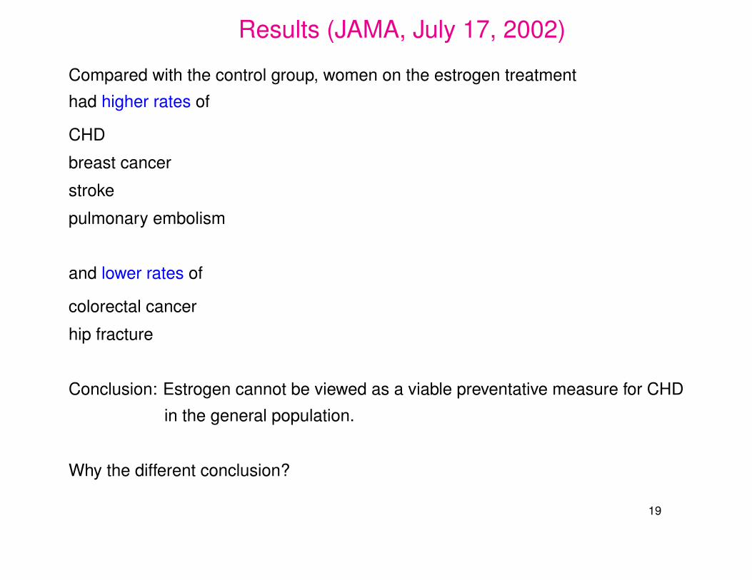
Results (JAMA, July 17, 2002)
Compared with the control group, women on the estrogen treatment
had higher rates of
CHD
breast cancer
stroke
pulmonary embolism
and lower rates of
colorectal cancer
hip fracture
Conclusion: Estrogen cannot be viewed as a viable preventative measure for CHD
in the general population.
Why the different conclusion?
19
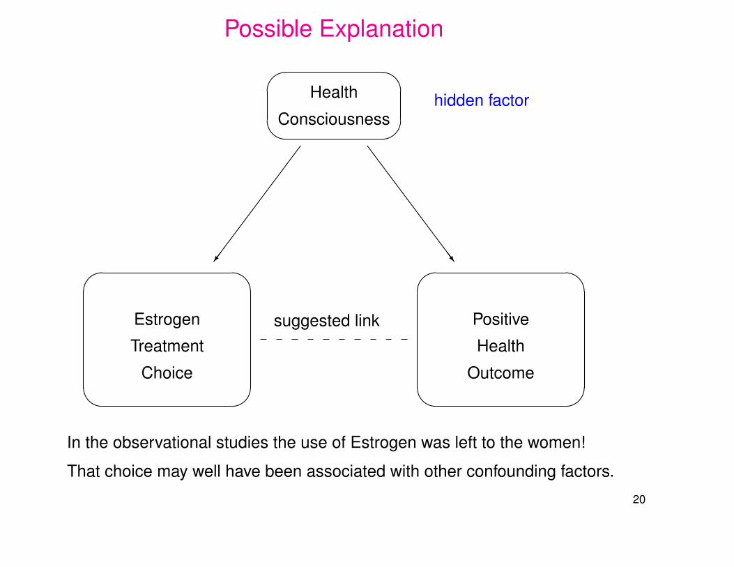
Possible Explanation'
&
$
%
'
&
$
%
'
&
$
%
suggested link
Health
Consciousnesshidden factor
Estrogen
Treatment
Choice
Positive
Health
Outcome
�������������/
SSSSSSSSSSSSSw
In the observational studies the use of Estrogen was left to the women!
That choice may well have been associated with other confounding factors.
20
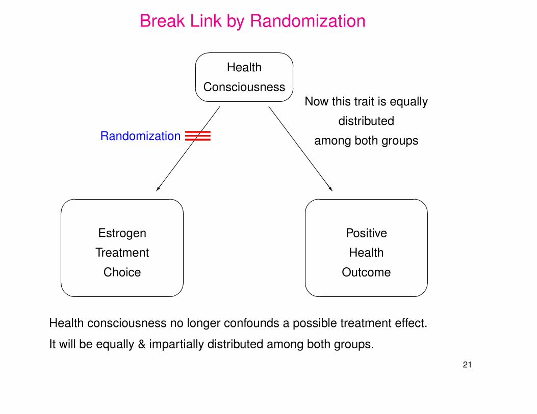
Break Link by Randomization'
&
$
%
'
&
$
%
'
&
$
%
Health
Consciousness
Estrogen
Treatment
Choice
Positive
Health
Outcome
�������������/
SSSSSSSSSSSSSw
———Randomization
Now this trait is equally
distributed
among both groups
Health consciousness no longer confounds a possible treatment effect.
It will be equally & impartially distributed among both groups.
21
Ethical Randomization IssuesSmoking and lung cancer.
Both could be linked to stress, an unmeasured variable.
Assigning “smoking” randomly is only viable in animal experiments.
But tests on animals appeared to rule out a link. (Didn’t inhale?)
One could attempt to measure stress on some scale.
However, this again runs into the hidden factor problem.
Health conscious people could be dealing with stress more effectively.
But there are these mucked up lungs and long time smokers living to 93.
Famous statisticians (Sir R.A. Fisher and Joseph Berkson) argued strongly against
a link between lung cancer & smoking.
22
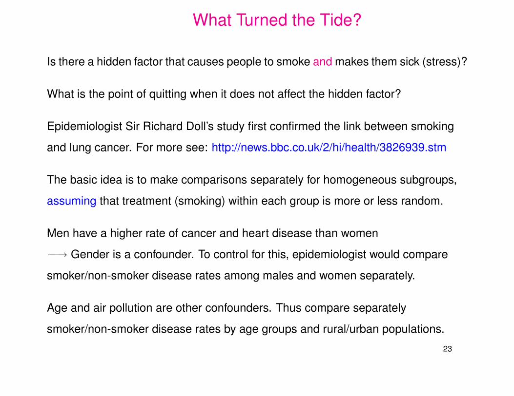
What Turned the Tide?
Is there a hidden factor that causes people to smoke and makes them sick (stress)?
What is the point of quitting when it does not affect the hidden factor?
Epidemiologist Sir Richard Doll’s study first confirmed the link between smoking
and lung cancer. For more see: http://news.bbc.co.uk/2/hi/health/3826939.stm
The basic idea is to make comparisons separately for homogeneous subgroups,
assuming that treatment (smoking) within each group is more or less random.
Men have a higher rate of cancer and heart disease than women
−→ Gender is a confounder. To control for this, epidemiologist would compare
smoker/non-smoker disease rates among males and women separately.
Age and air pollution are other confounders. Thus compare separately
smoker/non-smoker disease rates by age groups and rural/urban populations.
23
Interesting Tidbits from Sir Richard
In 1954, 80% of British adults smoked. Today, that figure is 26%.
“Mortality from lung cancer was increasing every year in the first few decades of
the last century,” said Sir Richard. “People didn’t pay any attention to these mortality
rates during the war.”
Sir Richard: “I personally thought it was tarring of the roads. We knew that there
were carcinogens in tar.”
“It wasn’t long before it became clear that cigarette smoking may be to blame.
I gave up smoking two-thirds of the way through that study.”
24

More
In 1951 the UK’s Medical Research Council asked 40,000 doctors if they smoked.
Over the course of the next three years, they compared those answers with
information about doctors who went on to develop lung cancer.
They found a direct link.
The findings prompted the then UK health minister Iain Macleod to call a
news conference. Chain-smoking throughout, he said: ”It must be regarded as
established that there is a relationship between smoking and cancer of the lung.”
The study has provided the foundation for all other research into the impact of
smoking cigarettes on health.
It has arguably helped to save millions of lives.
25

R.A. Fisher wrote his classic, The Design of Experiments,
in 1935. He opened his exposition with the most famous
experiment in statistical thinking, the lady-tasting-tea
experiment.
Hinkelmann and Kempthorne (1994), Design and Analysis of
Experiments, Volume I Introduction to Experimental Design.
It was a summer afternoon in Cambridge, England, in the
late 1920s. A group of university dons, their wives, and
some guests were sitting around an outdoor table for
afternoon tea. One of the women (Muriel Bristol)
was insisting that tea tasted different depending upon
whether the tea was poured into the milk or whether
the milk was poured into the tea. Salsburg (2001)
26
The Tea Tasting Experiment
The experiment consists in mixing 8 cups of tea, four in one way (A) and four in the
other (B), and presenting them to the Lady in a random order.
She has been told in advance that there will be 4 cups of each kind of preparation,
all 8 cups arranged in random order.
By tasting the 8 cups her task is to divide the 8 cups into two groups of 4
4“A’s” & 4 “B’s”, agreeing, if possible, with the treatments received.
There are(8
4)
= 8!/(4!)2 = 8 ·7 ·6 ·5/(1 ·2 ·3 ·4) = 7 ·2 ·5 = 70 ways of dividing
the 8 cups into two groups of 4, declaring which group belongs to which treatment.
By random choice the chance of getting it correct is 1/70 = 0.0143, rather unlikely,
but not extremely so. Note: 1/70 =(4
4)·(4
0)/(8
4).
27
Are We Too Stringent to Be Convinced?
Getting all 8 cups classified correctly is a strong requirement.
What if the Lady had gotten 3 correct A classifications and 1 B mistaken as an A?
The chance of that would be(4
3)·(4
1)/(8
4)
= 16/70 = .2286.
Is it a sufficiently convincing showing if the Lady gets at least 3 right?
Then by pure random choice the chance of that would be 17/70 = .2429,
no longer that unlikely.
To allow for some rare missteps of the Lady and still be impressed
by her performance one should have prepared more cups.
28
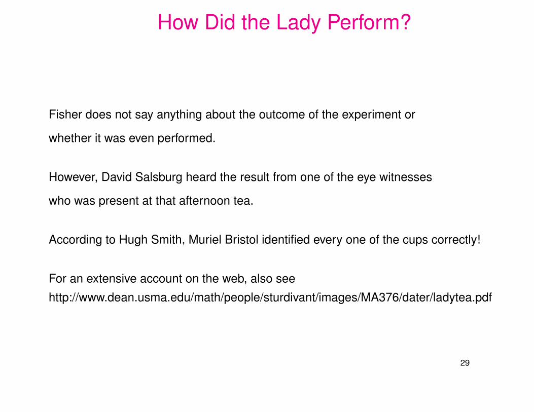
How Did the Lady Perform?
Fisher does not say anything about the outcome of the experiment or
whether it was even performed.
However, David Salsburg heard the result from one of the eye witnesses
who was present at that afternoon tea.
According to Hugh Smith, Muriel Bristol identified every one of the cups correctly!
For an extensive account on the web, also see
http://www.dean.usma.edu/math/people/sturdivant/images/MA376/dater/ladytea.pdf
29
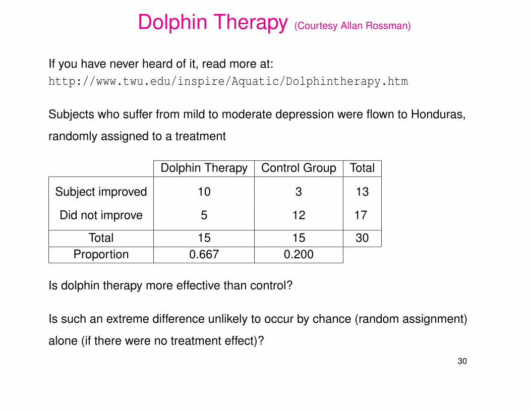
Dolphin Therapy (Courtesy Allan Rossman)
If you have never heard of it, read more at:http://www.twu.edu/inspire/Aquatic/Dolphintherapy.htm
Subjects who suffer from mild to moderate depression were flown to Honduras,
randomly assigned to a treatment
Dolphin Therapy Control Group Total
Subject improved 10 3 13
Did not improve 5 12 17
Total 15 15 30Proportion 0.667 0.200
Is dolphin therapy more effective than control?
Is such an extreme difference unlikely to occur by chance (random assignment)
alone (if there were no treatment effect)?
30
How to Assess the Chance Effect?
If there is no treatment effect, we could try to assess how likely chance alone,
splitting 30 subjects randomly into two groups of 15 (treatment) and 15 (control),
would split the 13 improvers such that at least 10 fall into the treatment group.
Take 30 cards, labeled 1,2,3, . . . ,30, shuffle them and deal them out in
two piles of 15 each (treatment and control).
Count the number Y of cards in the treatment pile with numbers ≤ 13
1,2, . . . ,13 represent the improvers, 14,15, . . . ,30 the non-improvers.
Repeat this process over and over many times, say N = 100000 times, and observe
the proportion of cases when chance alone gives us Y ≥ 10.
If this chance is very small we may be induced to lean towards a treatment effect.
31
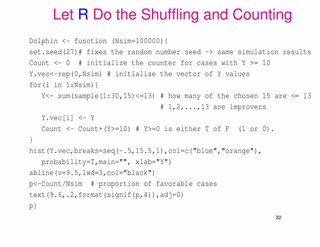
Let R Do the Shuffling and Counting
Dolphin <- function (Nsim=100000){
set.seed(27)# fixes the random number seed -> same simulation results
Count <- 0 # initialize the counter for cases with Y >= 10
Y.vec<-rep(0,Nsim) # initialize the vector of Y values
for(i in 1:Nsim){
Y<- sum(sample(1:30,15)<=13) # how many of the chosen 15 are <= 13
# 1,2,...,13 are improvers
Y.vec[i] <- Y
Count <- Count+(Y>=10) # Y>=0 is either T of F (1 or 0).
}
hist(Y.vec,breaks=seq(-.5,15.5,1),col=c("blue","orange"),
probability=T,main="", xlab="Y")
abline(v=9.5,lwd=3,col="black")
p<-Count/Nsim # proportion of favorable cases
text(9.6,.2,format(signif(p,4)),adj=0)
p}
32
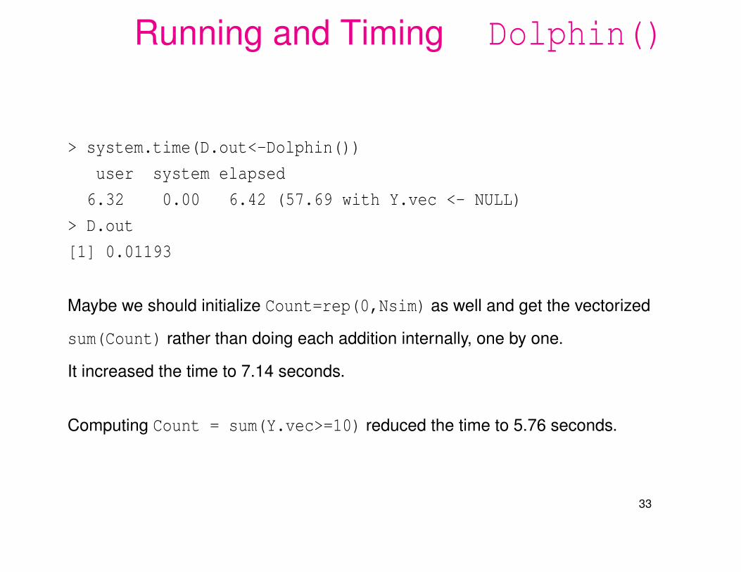
Running and Timing Dolphin()
> system.time(D.out<-Dolphin())
user system elapsed
6.32 0.00 6.42 (57.69 with Y.vec <- NULL)
> D.out
[1] 0.01193
Maybe we should initialize Count=rep(0,Nsim) as well and get the vectorized
sum(Count) rather than doing each addition internally, one by one.
It increased the time to 7.14 seconds.
Computing Count = sum(Y.vec>=10) reduced the time to 5.76 seconds.
33
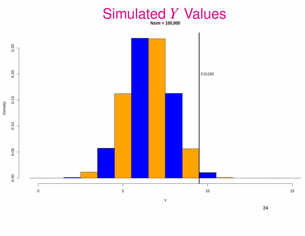
Simulated Y ValuesNsim = 100,000
Y
De
nsi
ty
0 5 10 15
0.0
00
.05
0.1
00
.15
0.2
00
.25
0.01193
34
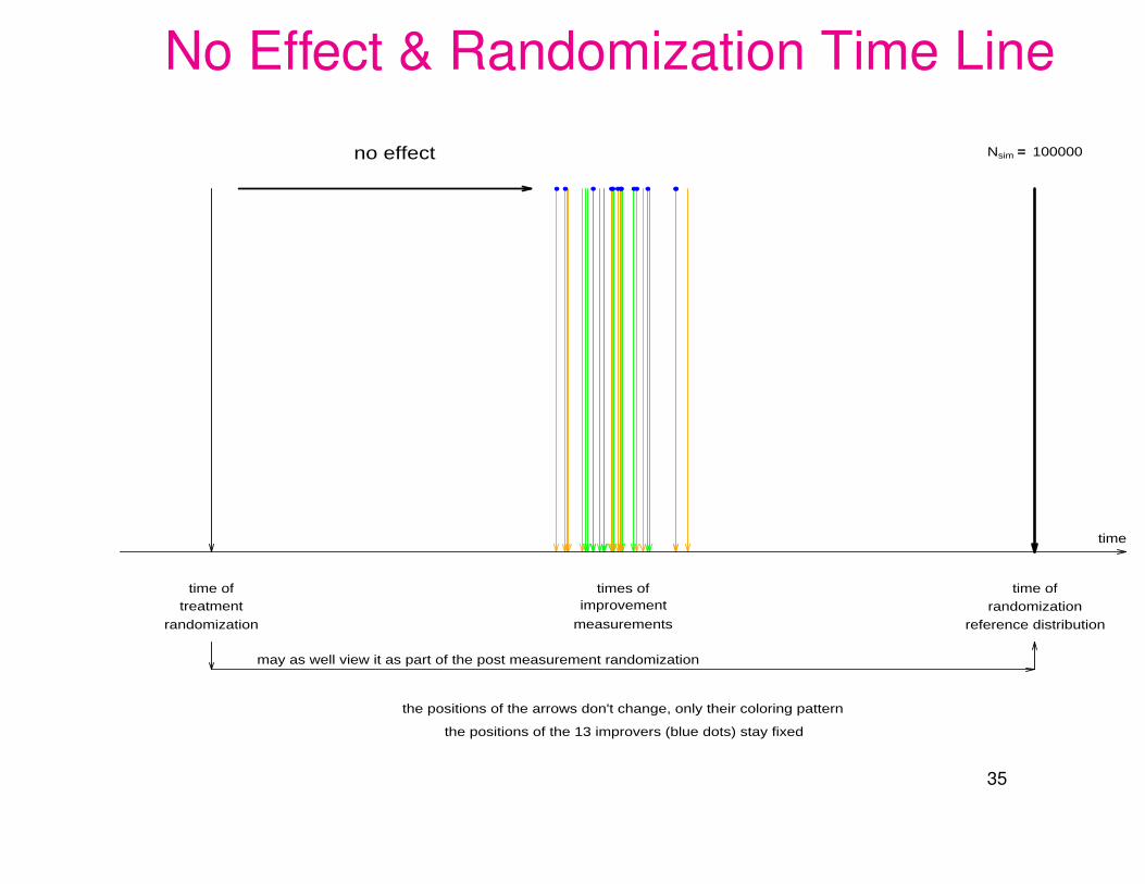
No Effect & Randomization Time Line
● ●● ●●● ●● ●●●●●
time
time oftreatment
randomization
times ofimprovement
measurements
time ofrandomization
reference distribution
no effect Nsim == 100000
may as well view it as part of the post measurement randomization
the positions of the arrows don't change, only their coloring pattern
the positions of the 13 improvers (blue dots) stay fixed
35

Statistical Significance
Chance alone would give us only a .01+ probability of seeing 10 or more of the
13 improvers in the treatment group of 15.
This is usually considered sufficiently rare to be called statistically significant.
=⇒ Something else but randomness seems to be at play here.
There seems to be some treatment effect (Induction).
The previous route via simulation (N = 100000) was chosen for its
operational appeal.
It emulates the random splits into two groups of 15 each, over and over.
However, there is a mathematical reasoning giving the exact probability.
36
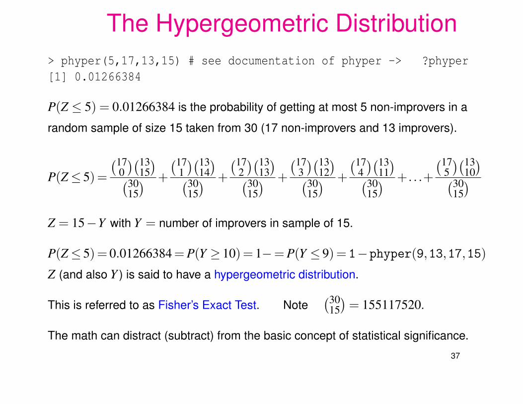
The Hypergeometric Distribution> phyper(5,17,13,15) # see documentation of phyper -> ?phyper[1] 0.01266384
P(Z ≤ 5) = 0.01266384 is the probability of getting at most 5 non-improvers in a
random sample of size 15 taken from 30 (17 non-improvers and 13 improvers).
P(Z≤ 5)=
(170)(13
15)(30
15) +
(171)(13
14)(30
15) +
(172)(13
13)(30
15) +
(173)(13
12)(30
15) +
(174)(13
11)(30
15) +. . .+
(175)(13
10)(30
15)
Z = 15−Y with Y = number of improvers in sample of 15.
P(Z≤ 5)= 0.01266384 = P(Y ≥ 10)= 1−= P(Y ≤ 9)= 1−phyper(9,13,17,15)Z (and also Y ) is said to have a hypergeometric distribution.
This is referred to as Fisher’s Exact Test. Note(30
15)
= 155117520.
The math can distract (subtract) from the basic concept of statistical significance.
37
The Role of Randomization
The random splitting of the 30 subjects into two groups of 15 (Dolphin Therapy and
Control) gives us a basis for viewing the observed result as just one of the 100000
simulations generated later on.
It gives us the simulation based context for our inductive reasoning.
When using the hypergeometric probability calculations, it gives us a
mathematical basis for carrying out the test and calculating the
significance probability of 0.01266384.
Without randomization in the original group splitting we cannot make the link to the
later simulations. We could only pretend that the groups were a random split.
38
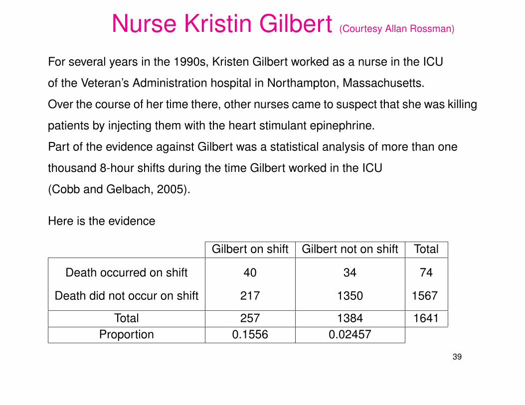
Nurse Kristin Gilbert (Courtesy Allan Rossman)
For several years in the 1990s, Kristen Gilbert worked as a nurse in the ICU
of the Veteran’s Administration hospital in Northampton, Massachusetts.
Over the course of her time there, other nurses came to suspect that she was killing
patients by injecting them with the heart stimulant epinephrine.
Part of the evidence against Gilbert was a statistical analysis of more than one
thousand 8-hour shifts during the time Gilbert worked in the ICU
(Cobb and Gelbach, 2005).
Here is the evidence
Gilbert on shift Gilbert not on shift Total
Death occurred on shift 40 34 74
Death did not occur on shift 217 1350 1567
Total 257 1384 1641Proportion 0.1556 0.02457
39
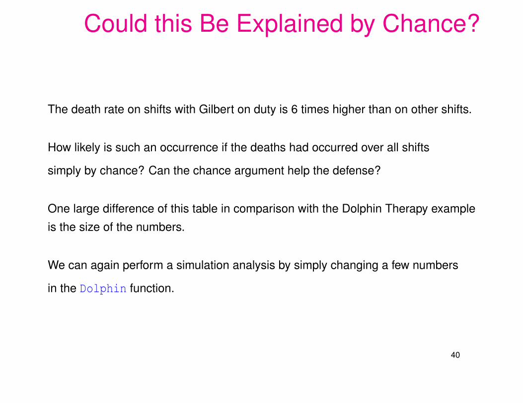
Could this Be Explained by Chance?
The death rate on shifts with Gilbert on duty is 6 times higher than on other shifts.
How likely is such an occurrence if the deaths had occurred over all shifts
simply by chance? Can the chance argument help the defense?
One large difference of this table in comparison with the Dolphin Therapy example
is the size of the numbers.
We can again perform a simulation analysis by simply changing a few numbers
in the Dolphin function.
40
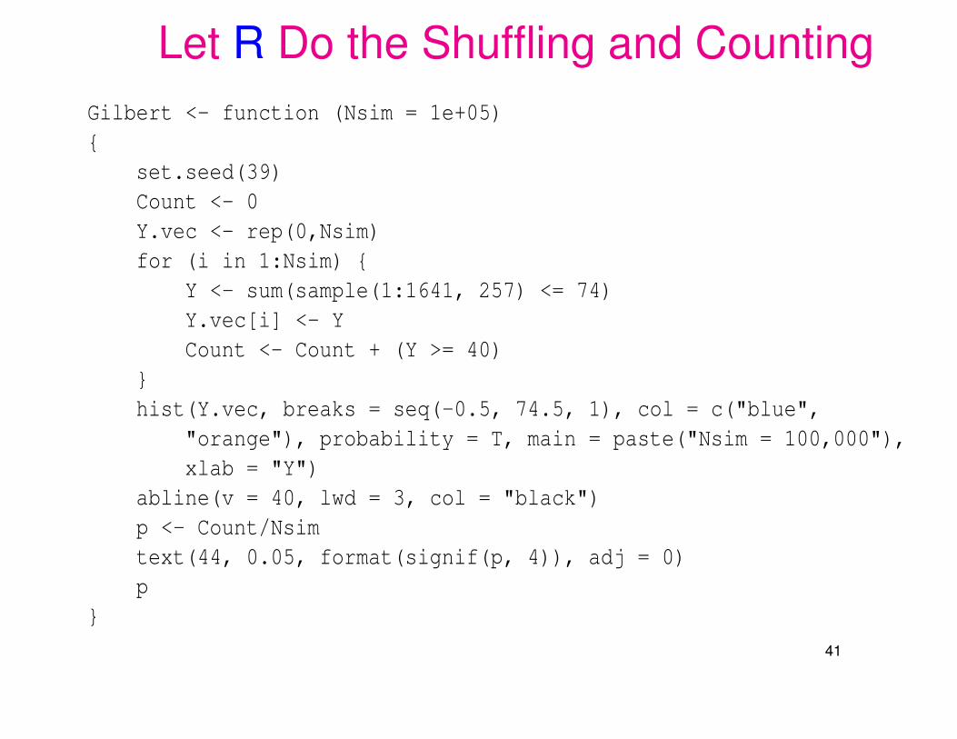
Let R Do the Shuffling and CountingGilbert <- function (Nsim = 1e+05){
set.seed(39)Count <- 0Y.vec <- rep(0,Nsim)for (i in 1:Nsim) {
Y <- sum(sample(1:1641, 257) <= 74)Y.vec[i] <- YCount <- Count + (Y >= 40)
}hist(Y.vec, breaks = seq(-0.5, 74.5, 1), col = c("blue",
"orange"), probability = T, main = paste("Nsim = 100,000"),xlab = "Y")
abline(v = 40, lwd = 3, col = "black")p <- Count/Nsimtext(44, 0.05, format(signif(p, 4)), adj = 0)p
}
41
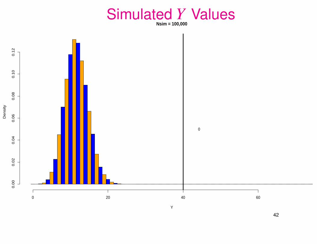
Simulated Y ValuesNsim = 100,000
Y
De
nsi
ty
0 20 40 60
0.0
00
.02
0.0
40
.06
0.0
80
.10
0.1
2
0
42
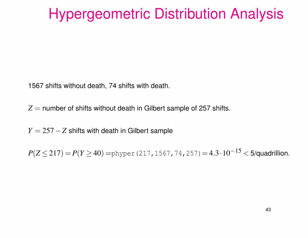
Hypergeometric Distribution Analysis
1567 shifts without death, 74 shifts with death.
Z = number of shifts without death in Gilbert sample of 257 shifts.
Y = 257−Z shifts with death in Gilbert sample
P(Z≤ 217)= P(Y ≥ 40)=phyper(217,1567,74,257)= 4.3·10−15 < 5/quadrillion.
43
Where Does Randomness Come from?The previous simulations and hypergeometric calculation invoke randomness.
Either the death shifts are randomly allocated to the Gilbert or non-Gilbert shifts,
or Gilbert’s shifts are randomly chosen from the total of shifts with or without deaths.
Either method would justify the simulation or hypergeometric calculation.
One basic assumption is that Gilbert is innocent and that chance is at work.
What Chance?
Gilbert was assigned to the shifts, possibly somewhat haphazardly or
by expressing a preference. Some randomness?
The deaths may allocate themselves somewhat randomly among all shifts.
Either way, not all allocations may be equally likely.
Night shifts may see more deaths, Gilbert may have worked more night shifts.
http://well.blogs.nytimes.com/2008/02/20/dying-on-the-night-shift/
There may be other confounding factors. The Defense can soften the blow.
44
Steps in Designing of Experiments (DOE)
1. Be clear on the goal of the experiment. Which questions to address?
Set up hypotheses about treatment/factor effects, a priori.
Don’t go fishing afterwards! It can only point to future experiments.
2. Understand the experimental units over which treatments will be randomized.
Where do they come from? How do they vary? Are they well defined?
3. Define the appropriate response variable to be measured.
4. Define potential sources of response variation
a) factors of interest
b) nuisance factors
5. Decide on treatment and blocking variables.
6. Define clearly the experimental process and what is randomized.
45
Three Basic Principles in Experimental DesignReplication:
repeat experimental runs under same values for control variables.⇒ can we approximately repeat effects?⇒ understanding inherent variability⇒ better response estimate via averaging.
Repeat all variation aspects of an experimental run.
Randomization:Confounding between treatment and other factors (hidden or not) unlikely.Removes sources of bias arising from factor/unit interaction.Provides logical/probability basis for inference about treatment effects.
Blocking:Randomized treatment assignment within blocks.Separates variation between blocks from treatment effect (variation within blocks).Most effective when blocks are homogeneous within and quite variable between.Makes treatment effect more clearly visible, i.e., increases test power.
46
You Have to Change Something!
Insanity: doing the same thing over and over again and expecting different results.
Albert Einstein, (attributed), physicist (1879 - 1955)
Of course, there is value in repetition:
Experience is recognizing the same mistake when you make it again.
47