applied mathematical modelling · development of generalized iwan model to simulate frictional...

Applied Mathematical Modelling xxx (2014) xxx–xxx

Contents lists available at ScienceDirect

Applied Mathematical Modelling

journal homepage: www.elsevier .com/locate /apm

Development of generalized Iwan model to simulate frictionalcontacts with variable normal loads

http://dx.doi.org/10.1016/j.apm.2014.01.0080307-904X/� 2014 Elsevier Inc. All rights reserved.

⇑ Corresponding author. Tel.: +98 21 77240198; fax: +98 21 77240488.E-mail address: [email protected] (H. Ahmadian).

Please cite this article in press as: M. Rajaei, H. Ahmadian, Development of generalized Iwan model to simulate frictional contacvariable normal loads, Appl. Math. Modell. (2014), http://dx.doi.org/10.1016/j.apm.2014.01.008

Majid Rajaei, Hamid Ahmadian ⇑Center of Excellence in Experimental Solid Mechanics and Dynamics, School of Mechanical Engineering, Iran University of Science and Technology, Narmak,Tehran 16848, Iran

a r t i c l e i n f o a b s t r a c t

Article history:Received 8 June 2013Received in revised form 12 October 2013Accepted 28 January 2014Available online xxxx

Keywords:Frictional contactsVariable normal loadIwan modelMasing rule

Most friction models are originally proposed to predict restoring forces in mechanical con-tacts with constant normal load. In practice the contact interface kinematics may involvenormal motion in addition to the tangential displacements, leading to variation of the con-tact normal load. This phenomenon is observed most strongly in contacts with high lateralvibration amplitudes and is known as slap. The current study establishes a general frictionmodel to account for variation in the normal load and enables one to predict the behaviorof a contact more precisely. Iwan model (1966) [5] is a suitable candidate for contact inter-face modeling and is able to represent the stick-micro/macro slip behavior involved in afriction contact. This physical based model is employed in the current work and its physicalparameters are generalized to include the normal load variation effects. The model is char-acterized by a slippage distribution density function and a linear stiffness at stick state.Both these parameters, defined in presence of constant normal load in the original model,are derived considering normal load variation leading to generalization of the contactmodel. Conventional models with constant normal loads produce symmetric contact inter-face hysteresis loops, but the developed generalized Iwan model is capable of generatingasymmetric hysteresis loops similar to those frequently seen in experiments. The general-ized contact model is employed to simulate the measured behavior of a beam with fric-tional support observed in an experimental test set-up. The contact slippage distributionfunction is first identified in a constant normal load condition. Next in low levels of contactpreloads where variation of the normal load is significant, the identified distribution func-tion in generalized form is employed to predict the experimental observations.

� 2014 Elsevier Inc. All rights reserved.

1. Introduction

Contact modeling is of considerable practical importance and occurs in many of mechanical systems. In recent decades, ithas been the focus of a number of studies. Investigating the dynamic behavior of mechanical systems often requires mod-eling contact between two or more components of the system and using detailed finite element models is quite complicatedand almost impossible to implement which generally leads to inaccurate predictions. In general, an experimental approachbased on the identification of contact parameters appears to be more favorable because of its efficiency.

ts with

http://dx.doi.org/10.1016/j.apm.2014.01.008

mailto:[email protected]


http://www.sciencedirect.com/science/journal/0307904X

http://www.elsevier.com/locate/apm


2 M. Rajaei, H. Ahmadian / Applied Mathematical Modelling xxx (2014) xxx–xxx

Surface roughness has a key role on contact interface attributes and is responsible for nonlinear characteristics of the con-tact, which can change the dynamic behavior of the system in different vibration amplitudes. The interface is in stick regimeat low vibration amplitudes, i.e. the system behaves linearly. As the response level increases, nonlinear mechanisms such asslippage and micro impact start to develop. Research works on contact friction characteristics have a rich history. Den Hartog[1] and Dowell [2] are the pioneers in this field followed by comprehensive investigations of friction phenomenon performedby Ferri [3] and Berger [4]. A large number of models have been developed to simulate the friction effects on mechanicalsystems. The Iwan model [5] is commonly used to model micro slip. It consists of networks of parallel Jenkin’s elementsallowing to model partial slip in the contact interface. There are other friction models offering smooth transition from stickto macro slip. The Dahl model [6], the Valanis model [7], the Leuven model [8,9] and LuGre friction model [10] are someexamples. Gaul and Lenz [11] performed an experimental study to verify the capability of the Valanis model. Segalman[12] inspected the validity of the Iwan model experimentally. Gaul and Nitsche [13] performed a comprehensive overviewon a range of constitutive models for contact interface mechanisms.

A contact model must be capable of taking into account the main nonlinear characteristics involved in the interface.Investigations on the contact dynamics are performed in three fields; the first is studying the friction characteristics in con-tact interface and only the tangential component of the contact force is considered and normal force assumed to be constant.All the mentioned models [1–13] fall in the first group. The application of these models is limited to contacts with simplegeometry and negligible normal motion. In these models the coupling of normal motion and tangential vibration at the inter-faces is ignored and the main outcome of this assumption is the symmetry of hysteresis loops. However in experimentalobservations asymmetric hysteresis loops are frequently seen indicating two returning curves of the hysteresis loops arenot following the same trend. These different curves are the result of normal load variations. The second field of study isinspecting the behavior of interface in normal direction and considers a frictionless contact. The application of this approachis limited to collision of multi-body systems or contact with perfectly frictionless surfaces [14,15]. And the third field isdeveloping a general contact model considering the interaction of normal and tangential vibration at the interface. Consid-ering impact and friction in contact interface, Han and Gilmore [16] employed static and kinetic coefficients of friction torelate normal and tangential components of the contact force in their model. A general regularized contact model is devel-oped by Gonthier et al. [17] which include normal compliance, energy dissipation and friction force using seven parameters.However these two models ignore the effect of normal load on tangential stiffness. Gaul and Mayer [18] used finite elementapproach to introduce an improved method to model contact interfaces. They adopted a nonlinear stiffness to model impactforce between the contact surfaces. Yang et al. [19] employed Jenkins element to investigate the effect of normal load onhysteresis loop which only describes the full-slip or full-stick situation. In all published articles simplifications are usedand to the authors knowledge there is no proper micro slip model capable of taking into account the effect of normal loadvariation to generate hysteresis loops observed in micro/macro slip region.

In this paper, a generalized Iwan model is developed. Original Iwan model is capable of reproducing the important contactproperties as they are now understood and many authors used this model to predict contact behavior in structures. Howeverthe applications of Iwan model are restricted to cases with constant level of normal force. The physical based parametricIwan model enables one to derive their characteristics directly from experimental data, and this is another reason foremploying the model in this investigation. The model is generalized to include the effect of normal load variation in the con-tact. This is achieved by special scaling of the distribution function and the shear stiffness variations.

The remainder of this paper is organized as follows: in Section 2 the generated force by Iwan model in presence of normalload variation is obtained and properties of derived model are discussed. Sections 3 and 4 describe the mathematical mod-eling of set-up and the test procedure respectively. In Section 5, Iwan distribution function in high preload condition is iden-tified. To ensure the validation of identified parameters two different identifications approaches based on the energydissipation function and the force state mapping are employed. In Section 6 by reducing the preload, identified model is usedto regenerate the measured data in variable preload.

2. Generalized Iwan contact model

Iwan’s model composed of an infinite number of spring-slider arrays, shown in Fig. 1, known as Jenkins elements [5]. Jen-kins element is an ideal elasto-plastic element, composed of a single discrete spring in series with a Coulomb damper with acritical slipping force. The Iwan model represents hysteretic features and models transitions in stick–slip states, which ap-pears in a contact. Applied tangential forces to the model, distributes between Jenkins elements and obligate sliders with lowcritical slipping forces to begin to saturate and slip. This phenomenon known as micro-slip causes softening effect and en-ergy dissipation at the contact interface. Increasing the applied force makes more sliders to slip, finally, at the ‘‘ultimateforce’’ all dampers would saturate and the full contact’s slip begins. Critical slipping force of frictional sliders f � is shownby a distribution density function uðf �Þ, thus uðf �Þdf � is the fraction of sliders which their critical slipping force is betweenf � and f � þ df �.

A typical Iwan model force–displacement hysteresis loop is shown in Fig. 2. The force required for deformation along thepath a–b, often referred to as ‘‘backbone curve’’, is:

Pleasevariab

fabðxÞ ¼Z kx

0f �uðf �Þdf � þ kx

Z 1

kxuðf �Þdf �; ð1Þ

cite this article in press as: M. Rajaei, H. Ahmadian, Development of generalized Iwan model to simulate frictional contacts withle normal loads, Appl. Math. Modell. (2014), http://dx.doi.org/10.1016/j.apm.2014.01.008


k/n

k/n

k/n

k/n

f

f

x

1*/n

f2*/n

f3*/n

fn*/n

Fig. 1. Iwan spring-slider model.

Fig. 2. A typical symmetrical hystresis loop.

M. Rajaei, H. Ahmadian / Applied Mathematical Modelling xxx (2014) xxx–xxx 3

where k is the spring stiffness and x is the displacement. The ‘‘returning curve’’ b–c–d in Fig. 2 is defined as:

Pleasevariab

fbcdðx;AÞ ¼ �Z kðA�xÞ

2

0f �uðf �Þdf � þ

Z kA

kðA�xÞ2

½kx� ðkA� f �Þ�uðf �Þdf � þ kxZ 1

kAuðf �Þdf �; ð2Þ

where A is the displacement amplitude and curve d–e–b, also shown in Fig. 2, is reflection of curve b–c–d. It’s known thevariation of normal load affects parameters of Iwan model. The two parameters of Iwan model are its distribution function,uðf �Þ, and the restoring stiffness, k. First we consider the change of the distribution function on generated force.

2.1. Variation effects of distribution function

The sliders in Iwan model are coulomb type and their saturation force is proportional to the normal load. Assuming thedistribution function uðf �Þ is obtained at a reference normal load, NRef, it is extended to other normal loads, N, by introducinga new parameter as:

aðtÞ ¼ NðtÞNRef

; ð3Þ

One may use the parameter a to dilate or compress the reference distribution function as:

uðf �;aÞ ¼ uðf �=aÞa

: ð4Þ

This means the distribution function varies during one cycle and the slider with saturation force of f � at reference normalload now may begin to slide at af �.

One needs to find how this variation during one cycle in Iwan model affects the contact restoring force. To answer thisquestion, a differential form is used to find the relation between the change in restoring force and the change of normalized




load ratio ðdaÞ and displacement ðdxÞ. Let us suppose the normal load ratio is increasing and in each step of displacement, thesliders with saturation force less than or equal to kx will slide. In constant preload, by increasing the displacement, the pop-ulation of saturated Jenkins elements increases as well but situation is different in the presence of variable normal load. Ascritical force of Jenkins elements are functions of preload, a rapid jump in preload may causes many or all Jenkins elementsgo to stick state. A criterion for this situation is considering the modified distribution function of Eq. (4) and to determine thechange in critical force of the strongest saturated Jenkins element from reference state due to incremental change of contactnormal load. These parameters for an element starts to slide at displacement x is:

Pleasevariab

f �@x ¼ kx ¼ af �@xRef : ð5Þ

Further increasing the displacement results:

f �@xþdx ¼ kðxþ dxÞ ¼ ðaþ daÞf �@xþdxRef : ð6Þ

As the reference critical force of the strongest saturated element which goes to slip increases, the population of saturationelements increases and vice versa. At da ¼ 0, one finds f �@xþdx

Ref > f �@xRef and in general cases:

da=a < dx=x ! f �@xþdxRef > f �@x

Ref : ð7Þ

Physical explanation of this relation is the relative change of restoring force in a particular element ðkdx=kxÞ should belarger than relative change in shear strength of that element ðda=aÞ. Satisfaction of this condition increases the percentageof saturated sliders, otherwise if this condition does not meet the sliders which were sliding at former state, go to stickingmode at xþ dx. In this situation there would be an element with critical force kxsðxs < xÞ which satisfies da=dx ¼ a=xs. Inphysical sense, the sliders with variable saturation force of equal or less than kxs remain in sliding mode and other sliderswould be at sticking region. The generated force by Jenkins element which is in first group is multiplied by da=a and added tokdx in the second group:

df ¼ daa

Z kxs

0f �

uðf �=aÞa

df � þ kdxZ 1

kxs

uðf �=aÞa

df �: ð8Þ

In this article we suppose the condition in Eq. (7) is always satisfied ðxs > xÞ. In other words normal load increases gradually.In this situation the strongest slider at current step starts to slide at next step, has saturation force kðxþ dxÞ=ð1þ da=aÞ andthe differential force is:

df ¼ daa

Z kx

0f �

uðf �=aÞa

ulastðf �Þdf � þZ k xþdx

1þda=a

kxðf �ð1þ da=aÞ � kxÞuðf

�=aÞa

df � þ kdxZ 1

k xþdx1þda=a

uðf �=aÞa

df �

¼ daa

Z kx

0f �

uðf �=aÞa

df � þ kdxZ 1

kx

uðf �=aÞa

df �: ð9Þ

Analytical integration of Eq. (9) by a change of variables leads to:

f ðxÞ ¼ aZ kx=a

0f �uðf �Þdf � þ kx

Z 1

kx=auðf �Þdf �: ð10Þ

On the other hand with decrease of normal load ratio, slipping sliders do not change their state but their slip force de-clines by the ratio of da=a and sliders which change their state from stick to slip have a maximum saturation force ofkðxþ dxÞ=ð1þ da=aÞ. This leads to the same equation derived for increasing normal load and as a result Eq. (9) can be usedfor any arbitrary loading pattern and there is no condition or limitation in decreasing pattern.

Eqs. (5)–(10) describe the initial loading pattern of the contact model and form the backbone curve. Next a relation forreturning curve is developed using the Masing rule. This rule states that the returning force is composed of the force atreturning point and double stretched backbone curve force:

f ðxÞ ¼ f ðx0Þ � 2Z kðx�x0Þ=2

0f �uðf �Þdf � � kðx� x0Þ

Z 1

kðx�x0Þ=2uðf �Þdf �; ð11Þ

where subscript ()0 denotes the value of parameter in returning point. It is seen the saturation force in the integrals limitsequals kðx� x0Þ=2; as part of displacement ðxrÞ returns the springs to the free-state and after that, other part ðxtÞ pulls themin opposite direction:

x� x0 ¼ xr þ xt : ð12Þ

If there was no change in normal load, these two parts would be equal ðxr ¼ xtÞ:

x� x0 ¼ 2xt ! xt ¼ ðx� x0Þ=2; ð13Þ

and limits of the integrals would be kxt : But when normal load varies one finds:

xt ¼aa0

xr ! xt ¼x� x0

1þ a0=a: ð14Þ




The differential change of restoring force equals:

Pleasevariab

df ¼ daa

Z kðx�x0Þ=1þa0=a

0f �

uðf �=aÞa

df � þ kdxZ 1

kðx�x0Þ=1þa0=a

uðf �=aÞa

df �: ð15Þ

Integrating both sides of Eq. (9) and considering the value of integration at initial point one arrives at:

f ðxÞ ¼ f ðx0Þ � ðaþ a0ÞZ kðx�x0Þ=aþa0


Z 1

kðx�x0Þ=aþa0

uðf �Þdf �: ð16Þ

2.2. The effects of stiffness variations on contact restoring force

Considering the influence of stiffness variation, which is a function of normal load itself in Iwan restoring force modelðk ¼ kðaÞÞ; one obtains the following condition:

jdx=xjP jdk=kj: ð17Þ

This condition ensures us the reverse sliding doesn’t happen. To understand this phenomenon, consider a saturated Jenkinselement, shown in Fig. 1, is pulled to the right direction and its slider is drawing in the same direction, now if the direction ofdisplacement changes (passing the returning point) and at the same time, stiffness has a sudden increase, slider slips in theright direction to reduce the elongation of spring and will make the same critical force as before, this slippage is in the oppo-site direction of the current displacement and is called reverse sliding.

As the stiffness is changed, the backbone curve remains in the original form and no modification is required. However todetermine the returning curve from Masing rule some difficulty arises. For instance when the stiffness of particular Jenkinselement reduces, the force changes depend on the position of the slider with respect to its reference point. The Masing’s formof the element is:

f ðxÞ ¼ f ðx0Þ � b1

Z b2x


Z 1

b2xuðf �Þdf �; ð18Þ

where b1 and b2 are unknown. To obtain these parameters we use the original relation for returning curve as:

f ðxÞ ¼ �Z kðA�xÞ

2

0f �uðf �Þdf � þ k

Z kA

kðA�xÞ2

x� ðA� f �=kÞ½ �uðf �Þdf � þ kxZ 1

kAuðf �Þdf �; ð19Þ

The first integral defines parts of forces generated by saturated elements, second integral represent forces of elementssaturated in initial loading and now are at x in elastic mode and finally the last integral refers to the elements never be sat-urated. The limits of integrals are function of k which varies in a loading cycle. These limits are defined using the propertiesof the element at the returning point as follows. In each saturated Jenkins element with constant normal load the elongationof spring is constant ðxc ¼ f �=kÞ: As normal load varies, this elongation changes over the loading path and at the returningpoint it would be f �=k0: We consider the displacement from returning point as sum of two parts defined in Eq. (12):

f � ¼ k0xr ¼ kxt ! xt ¼x� x0

1þ k=k0: ð20Þ

Eq. (20) specifies the upper limit of the first integral and lower limit of second integral as:

kxt ¼kk0ðx� x0Þ

kþ k0: ð21Þ

The upper limit of second integral is k0A as long as it is less than kxt : Moreover the integrant in second integral must bemodified from A� f �=k, the elongation of springs at returning point, to A� f �=k0. Applying these modifications, the returningcurve relation defined in Eq. (19) is rewritten as:

f ðxÞ ¼ �Z kk0 ðA�xÞ

kþk0

0f �uðf �Þdf � þ k

Z k0A

kk0 ðA�xÞkþk0

½x� ðA� f �=k0Þ�uðf �Þdf � þ kxZ 1

k0Auðf �Þdf �: ð22Þ

Direct employment of Eq. (22) faces two difficulties:

(I) One must insure the inequality kk0ðA�xÞkþk0

6 k0A is satisfied,(II) The amplitude A is meaningful in steady state response but not applicable in transient response.

Therefore it is more convenient to calculate the restoring force from Masing rule, and Eq. (22) may be defined in Masingform as:

f ðxÞ ¼ kk0

f ðx0Þ � 1þ kk0

� �Z kk0kþk0ðx�x0Þ


Z 1

kk0kþk0ðx�x0Þ





Comparing Eqs. (23) and (18), it becomes clear why the original form of Masing rule could not be used and we call the aboveform the adjusted Masing rule.

2.3. Combined effects of the stiffness and distribution function variations

The final step is to combine these results together and consider both effects of normal load on the distribution functionand the stiffness. Rewriting Eq. (16) in original Iwan form:

Fig. 3.(right).

Pleasevariab


1þa0=a

0f �

uðf �=aÞa

df � þ kZ a

a0kA

kðA�xÞ1þa0=a

x� A� a0f �

ka

� �� uðf �=aÞ

adf � þ kx

Z 1

aa0

kA

uðf �=aÞa

df �; ð24Þ

and combining it with Eq. (22), leads to:


1þka0k0a

0f �

uðf �=aÞa

df � þ kZ a

a0k0A

kðA�xÞ

1þka0k0a

x� A� a0f �

k0a

� �� uðf �=aÞ

adf � þ kx

Z 1

aa0

k0A

uðf �=aÞa

df �: ð25Þ

Then the final form of adjusted Masing rule can be written as:

f ðxÞ ¼ kk0

f ðx0Þ � aþ kk0

a0

� �Z kk0ka0þk0aðx�x0Þ


Z 1

kk0ka0þk0aðx�x0Þ


It’s worth mentioning based onEq. (7) limiting criterion for this relation is:

dxx

��P da

a� dk

k

��: ð27Þ

However for small change of normal load, provided the variation of stiffness is a linear function of normal load i.e.aðtÞ ¼ bkðtÞ where b ¼ constant; results jda=a� dk=kj ¼ 0 and criterion (27) is automatically satisfied.

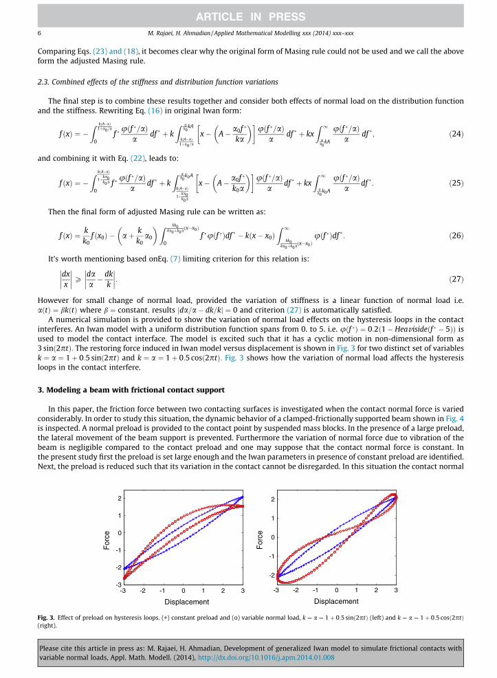
A numerical simulation is provided to show the variation of normal load effects on the hysteresis loops in the contactinterferes. An Iwan model with a uniform distribution function spans from 0. to 5. i.e. uðf �Þ ¼ 0:2 1� Heavisideðf � � 5Þð Þ isused to model the contact interface. The model is excited such that it has a cyclic motion in non-dimensional form as3 sinð2ptÞ: The restoring force induced in Iwan model versus displacement is shown in Fig. 3 for two distinct set of variablesk ¼ a ¼ 1þ 0:5 sinð2ptÞ and k ¼ a ¼ 1þ 0:5 cosð2ptÞ: Fig. 3 shows how the variation of normal load affects the hysteresisloops in the contact interfere.

3. Modeling a beam with frictional contact support

In this paper, the friction force between two contacting surfaces is investigated when the contact normal force is variedconsiderably. In order to study this situation, the dynamic behavior of a clamped-frictionally supported beam shown in Fig. 4is inspected. A normal preload is provided to the contact point by suspended mass blocks. In the presence of a large preload,the lateral movement of the beam support is prevented. Furthermore the variation of normal force due to vibration of thebeam is negligible compared to the contact preload and one may suppose that the contact normal force is constant. Inthe present study first the preload is set large enough and the Iwan parameters in presence of constant preload are identified.Next, the preload is reduced such that its variation in the contact cannot be disregarded. In this situation the contact normal

-3 -2 -1 0 1 2 3-3

-2

-1

0

1

2

Displacement

For

ce

-3 -2 -1 0 1 2 3

-2

-1

0

1

2

Displacement

For

ce

Effect of preload on hysteresis loops. (+) constant preload and (o) variable normal load, k ¼ a ¼ 1þ 0:5 sinð2ptÞ (left) and k ¼ a ¼ 1þ 0:5 cosð2ptÞ



F(t)( , )w x t

Fn(t)

PL

S nk

Fig. 4. The schematic view of beam.


force is not known and varies periodically due to harmonic external excitations. The contact normal force variations needs tobe considered in the modeling of the system and must be identified to predict the tangential contact force.

Euler–Bernoulli beam theory is employed to model the dynamic response of the beam. The beam has a modulus of elas-ticity of E, cross sectional moment of inertia of I, mass density of q, cross sectional area of �A, and length of L. In the modelaxial inertial effects of beam are neglected as the dynamic behavior is considered in a frequency range much lower than itsfirst axial mode. Therefore, in axial direction the beam is regarded as a spring of stiffness kb which is equal to E�A=L. The fric-tional support is composed of a pin welded to the right end of the beam and is allowed to slip on a steel block. The pin has aradius of r, mass of mp, mass moment of inertia of Jp. Applying a normal force to the rod provides a preload to the contactinterface. This is achieved, as shown in Fig. 5, by suspended mass blocks attached to the rod via a string. The beam is excitedby concentrated force F(t) applied at distance S from clamped end.

The beam equation of motion is:

Pleasevariab

EI@4w@x4 � FnlðtÞ

@2w@x2 þ q�A

@2w@t2 ¼ FðtÞdðx� SÞ � rFnlðtÞd0ðx� LÞ: ð28Þ

where Fnl(t) is the non-linear friction force at the contact. The normal stiffness of the contact interface is proportional to thecontact preload. It is assumed, within the range of preload variations in the current study, this relation is linear and is rep-resented with stiffness kn located between two contact surfaces. The beam is clamped at one side and loaded with shear forceat the other side. The shear force at beam frictional support can now be established using three terms, a static preload equalto total weight of suspended masses, preload variation caused by relative lateral movement of surfaces and inertia force ofblock masses,

EI@3wðL; tÞ@x3 ¼ knwðL; tÞ þ nbm

@2wðL; tÞ@t2 � g

!; ð29Þ

where nb is the number of blocks and m = 7 kg is the mass of each of them.One may solve Eq. (28) with the given boundary conditions to obtain the non-linear friction force Fnl(t). The friction force

and the shear deformation at the contact interface are needed to define hysteresis loops of the contact interface. The contactshear deformation is governed by three different effects included in the right hand side of the following identity:

uðtÞ ¼ �12

Z L

0

@wðx; tÞ@x

� �2

dxþ r@wðL; tÞ@x

þ FnlðtÞL�AE

: ð30Þ

Fig. 5. Test set-up.




The first effect is related to shortening of the beam due to its lateral bending motion and is described by the first term on theright hand side of Eq. (30). The second term is the relative motion due to rotation of the beam end, and last term indicates theaxial deformation of beam due to friction force at the contact interface.

To reduce the order of the nonlinear model of Eq. (28), the Galerkin method is employed. The friction in contact is dis-placement dependent phenomenon and corresponding base linear system mode shapes are function of amplitude. The non-linear response of the beam is expanded using the mode shapes of the base linear system as:

Pleasevariab

wðx; tÞ ¼Xn

i¼1

~/iðx; aÞqiðtÞ; ð31Þ

where a is the amplitude of response at direct measurement point. Employing this expansion series in Eq. (28) and usingtheir orthogonally properties, the discretized nonlinear equations of beam motion are:

€qiðtÞ þx2i ðaÞqiðtÞ � FðtÞ~/iðS; aÞ � khðaÞ

Xn

r¼1

qrðtÞ@~/rðL; aÞ

@x

!@~/iðL; aÞ

@x

¼ rd~/iðL; aÞ

dx�Xn

r¼1

qrðtÞZ L

0

@~/rðx; aÞ@x

@~/iðx; aÞ@x

dx

!FnlðtÞ � ~/iðL; aÞðknwðL; tÞ � nbmgÞ; i ¼ 1;2; . . . ;n: ð32Þ

where khðaÞ is the support equivalent flexural stiffness at different vibration levels. In the following section, experiments onthe structure shown in Fig. 4 are performed. The observed behavior of test structure is used to determine the mode shapes ofthe base linear system, the frictional and normal contact forces.

4. Experimental case study

The experimental case is a steel beam clamped at one end and fixed at other end with frictionally support as shown inFig. 5. The dimension of beam are L = 600 mm (length), b = 40 mm (width) and h = 5 mm (thickness). The rod attached to theend of beam end is steel and it has a radius of r = 5 mm and has the length the same as the beam width. The weight of sus-pended mass block provides the desired value for preload and this allows for the application of arbitrary preloads on thecontact interface. A B&K4200 mini shaker is used to excite the beam through a stinger at distance S = 550 mm from theclamped side. A B&K8200 force transducer is located between the beam and stinger to measure the excitations. Three accel-erometers AJB 120 are mounted on structure to measure the lateral acceleration and placed at distance x1 = 550 mm,x2 = 300 mm and x3 = 50 mm from clamped side. A laser Doppler OMETRON vh-1000-d is employed to measure axial defor-mation of beam at frictional end.

Two parameters of Iwan model, namely the stiffness of Jenkins elements, i.e. the stiffness of contact at stick state, and thedistribution function must be identified. To identify the stiffness at the stick state, the beam is excited with a low amplituderandom signal and frequency response function (FRF) is measured. The FRFs of the beam for two different preloads is shownin Fig. 6. In the mathematical model, the stiffness at contact is tuned in such a way to regenerate the same resonancefrequencies.

The identification of distribution function is more complicated. There are a few approaches for extracting this function.Song et al. [20] and Shiryayaev et al. [21] applied neural network method to identify the parameter of a uniform distributionfunction from time domain response. Segalman [22,23] proposed the distribution function with four unknown parameters.Ahmadian et al. [24] applied the force state mapping method to identify the hysteresis loop on contact interfere which couldbe used to identify the Iwan parameters. It is shown in the previous work of the authors that the distribution function couldbe identified by dissipation energy pattern in different displacement amplitude [25].

50 100 150 200 250

10-4

10-2

100

Frequency (Hz)

Iner

tanc

e (L

og M

ag)

One mass bblockThree mass blocks

Fig. 6. Linear frequency response curve for direct measurement.




All of these methods are restricted to the cases with constant preload. To provide this condition, we used three massblocks (21 kg) as the preload and two later approaches is employed at the same time to validate the identified distributionfunction.

5. Distribution function identification in a high preload

In test strategies of nonlinear systems it is common to excite the structure near one of its resonances using a single har-monic force. This practice leads to a dominant single mode response in systems without modal interaction and the contri-bution of other modes is usually marginal.

The measured force and acceleration signals are used to reconstruct the nonlinear restoring forces and shear deformationin the contact interface. The first part of this section deals with determination of the shape functions used in Galerkin pro-jection. Then the measured accelerations and identified shape functions are employed to calculate the generalized coordi-nates using Eq. (31).

The response of the structure contains one dominant harmonics close to the first natural frequencies of the system. There-fore, the mode shapes of the base linear system are good approximations for series expansion base functions. As mentionedin previous section, when the structure behaves linearly the contact interface is modeled by tangential spring. Eliminatingnonlinear parts of Eq. (28) and replacing the last term with kh leads to a linear equation of motion. This stiffness identifiedfrom test result and selected in such a way to regenerate resonance frequencies observed in the test.

It should be noted in Eq. (28) that the effect of accelerometers is not introduced for simple understanding but they areconsidered in the model. Using the section at place of each accelerometer, the beam divides into four parts and compatibilityrequirements at the interface of each two parts are added to the equations of motion. It is assumed that the displacementsand slopes at the sections don’t change but the shear forces and bending moments alter due to mass and inertia of the accel-erometers and the force transducer. Now, the linear base system is completely described. Having the linear mode shape, thegeneralized coordinate vector can be calculated using the measured accelerations at 3 points:

Pleasevariab

€qðtÞ ¼€q1ðtÞ€q2ðtÞ€q3ðtÞ

8><>:

9>=>; ¼

~/1ðx1; aÞ; ~/2ðx1; aÞ; ~/3ðx1; aÞ~/1ðx2; aÞ; ~/2ðx2; aÞ; ~/3ðx2; aÞ~/1ðx3; aÞ; ~/2ðx3; aÞ; ~/3ðx3; aÞ

264

375�1 €wðx1; tÞ

€wðx2; tÞ€wðx3; tÞ

8><>:

9>=>; ¼ U�1 €w: ð33Þ

Next we turn our attention to the experimental results. The mode shapes of the base linear system are inherently goodapproximation. Therefore, we donot expect a large number of modes contributing to construct the desired shape functionsand the number of mode shapes in Eq. (31) is set to be three. In other words, three linear mode shapes used to identify oneshape functions. The corresponding generalized coordinates q(t) of this three modes is shown in Fig. 7. As it is seen in thethird linear mode has a marginal contribution in the final shape functions that ensures that there is no need for more modesin construction of the desired shape functions.

The normal stiffness kn is the last parameter to be evaluated. The response of structure is insensitive to this parameter soit cannot be calculated by any identification method accurately. Johnson [26] showed that force–displacement for an infinitecylinder on a plane in normal direction would be:

d ¼ P1� m2

pEð2 lnð4r=a1Þ � 1Þ; a2

1 ¼ 4Pr=pE�; ð34Þ

0 0.01 0.02 0.03 0.04 0.05 0.06 0.07 0.08-4

-3

-2

-1

0

1

2

3

4

Time (s)

Gen

eral

ized

coo

rdin

ate

(m) q

1(t)

q2(t)

q3(t)

x 10-4

Fig. 7. A generalized coordinate at 30 m/s2 for direct measurement.




where P is the compressive load per unit, E and E� are elasticity modulus and elasticity composite modulus, respectively, r isthe radius of cylinder and v is the poison ratio. This relation plotted in Fig. 8 for dimension of the cylindrical rod which at-tached to the beam end. As it is shown a linear spring gives good estimate for this relation.

However infinite length of cylinder and frictionless of surfaces are two assumptions in Eq. (34) and calculated value forstiffness are rough but we use it in our model. That is because as mentioned above structure response is insensitive to thisparameter which means EIw00ðL; tÞ or beam support shear force remains invariant. It is shown in Eq. (29) shear force at beamend is summation of three terms which the effect of inertia force of mass blocks is negligible, this leads to the conclusion thatthe generated force by variation of normal spring remains the same and if spring stiffness decreases a few percent, the dis-placement amplitude increases in such way to make up this change in generated force. In other words when the normal stiff-ness exceeds from the certain value, the boundary condition at beam end becomes close to the classical simply supportboundary condition (rotation resistance due to friction exists anyway) and changing stiffness has no effect on supportreactions.

Another way to identify distribution function is by using contact dissipation energy [25]. It is shown that each distribu-tion function causes a unique pattern of dissipation energy in different amplitude and the relation is as follows:

Fig. 8

Pleasevariab

d2D

dA2 ¼ 4Ak2uðkAÞ; ð35Þ

where D is the dissipation energy. Increasing the number of recorded points increases the accuracy of identified function.This approach is less sensitive to noise than force state mapping method. Because in the later one, the nonlinear force is dif-ferentiation of two bigger terms (stiffness and inertia force) and noisy data leads to erroneous result.

In this paper, the single sinusoidal excitation is applied to beam at 80 different amplitudes to generate acceleration withamplitude from 40 mg to 6 g at direct point of measurement. In each level, the frequency of excitation is set to the resonancefrequency of structure on that level (with overall error 0.1 Hz). This frequency decreases from 57.3 Hz at 40 mg to 54.8 Hz at6 g. By having contact displacement and contact dissipation energy and using Eq. (35), the distribution function could beextracted.

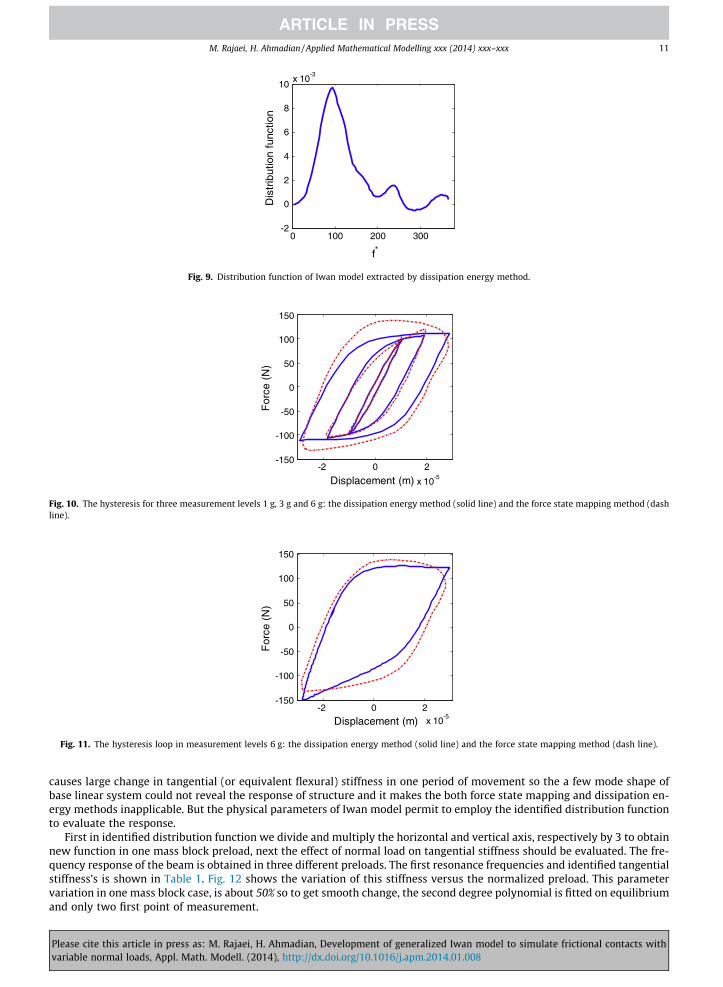
In Fig. 9 the distribution function identified by dissipation energy method is shown and hysteresis loop in contact forthree different amplitude levels by both methods is shown in Fig. 10. These diagrams have a good agreement at amplitudelevels up to 3 g after that normal load variation makes diagram to deviate from each other. Therefore if we seek for a reliabledistribution function, we could only take some part of this function which normal load effects doesnot contaminate it. In 3 gamplitude level a critical force of the strongest Jenkins element would be:

f � ¼ Ajoint � k ¼ 18� 10�6 � 11:02� 10þ6 ’ 200 N: ð36Þ

As it is shown, the deviation between two diagram starts at hysteresis loop end in 3 g level so we could conclude that thedistribution function are reliable and almost exact until 200 N on critical force axis.

In dissipation energy method The distribution function extracted on constant normal load assumption because the effectof this variation on dissipation energy is not considered therefore the hysteresis loops are plotted under this condition andvariation of normal load neglected but it’s worth to mention, if we accept the identified function as an exact one in wholespan and taking into the account the influence of normal on generated hysteresis loop, it could be seen that a better agree-ment between two methods would achieve (Fig. 11) although some deviations remain but it can capture some features.

6. Application of generalized Iwan model

In this section the preload of beam under the test reduces to one mass block and the identified distribution function isapplied to regenerate the time domain response of structure in high variation of normal load. The high variation of preload

. Force versus displacement in normal direction. r ¼ 5 mm; E ¼ 210 Mpa; v ¼ 0:3; L ¼ 0:05 m The slope of fitted line is kn ¼ 2:72� 109 kN=mm.



0 100 200 300-2

0

2

4

6

8

10x 10

-3

f*

Dis

trib

utio

n fu

nctio

nFig. 9. Distribution function of Iwan model extracted by dissipation energy method.

-2 0 2-150

-100

-50

0

50

100

150

Displacement (m)

For

ce (

N)

x 10-5

Fig. 10. The hysteresis for three measurement levels 1 g, 3 g and 6 g: the dissipation energy method (solid line) and the force state mapping method (dashline).

-2 0 2x 10

-5

-150

-100

-50

0

50

100

150

Displacement (m)

For

ce (

N)

Fig. 11. The hysteresis loop in measurement levels 6 g: the dissipation energy method (solid line) and the force state mapping method (dash line).


causes large change in tangential (or equivalent flexural) stiffness in one period of movement so the a few mode shape ofbase linear system could not reveal the response of structure and it makes the both force state mapping and dissipation en-ergy methods inapplicable. But the physical parameters of Iwan model permit to employ the identified distribution functionto evaluate the response.

First in identified distribution function we divide and multiply the horizontal and vertical axis, respectively by 3 to obtainnew function in one mass block preload, next the effect of normal load on tangential stiffness should be evaluated. The fre-quency response of the beam is obtained in three different preloads. The first resonance frequencies and identified tangentialstiffness’s is shown in Table 1. Fig. 12 shows the variation of this stiffness versus the normalized preload. This parametervariation in one mass block case, is about 50% so to get smooth change, the second degree polynomial is fitted on equilibriumand only two first point of measurement.

Please cite this article in press as: M. Rajaei, H. Ahmadian, Development of generalized Iwan model to simulate frictional contacts withvariable normal loads, Appl. Math. Modell. (2014), http://dx.doi.org/10.1016/j.apm.2014.01.008


Table 1The effect of preload on the contact tangential stiffness.

Number of mass blocks One mass block Two mass blocks Three mass blocks

Fundamental frequency 55.3 Hz 56.52 Hz 57.3 HzTangential stiffness 4:90� 106 N=m 8:71� 106 N=m 11:02� 106 N=m

0 1 2 30

2

4

6

8

10

12x 10

6

Normalized preload (N/N)

Tan

gent

ial s

tiffn

ess

(N/m

)

5.44*106α-5.45*105α2

Fig. 12. The identified tangential stiffness for three points (circles) and fitted curve to estimate curve between two first points (solid line).

-1 0 1

x 10-5

-40

-20

0

20

40

Displacement (m)

For

ce (

N)

Fig. 13. The model generated hysteresis loop.

0 0.02 0.04 0.06 0.08-20

-10

0

10

20

Time (s)

Acc

eler

atio

n (m

/s2 )

Fig. 14. Time domain for direct measurement: test data (solid line) and model prediction (dash line).


The generated hysteresis loop is shown in Fig. 13 and to validate the model, the time domain response in direct point ofmeasurement shown in Fig. 14.

By increasing the amplitude, the test result and model prediction diverge from each other. There are two main causes forit, first, the normal spring which is used to model normal load variation is acceptable in limited band and increasing the

Please cite this article in press as: M. Rajaei, H. Ahmadian, Development of generalized Iwan model to simulate frictional contacts withvariable normal loads, Appl. Math. Modell. (2014), http://dx.doi.org/10.1016/j.apm.2014.01.008



amplitude activates the phenomenon like micro slap and its strong nonlinear effects influence on beam response. Secondcause is the domain of reliability of distribution function. As we mentioned the original identified function is reliable until18� 10�6m for tangential displacement amplitude which leads to Jenkins elements with critical force up to 200 N. When thepreload reduces, the critical force of this Jenkins elements decrease to one-third of original value but the stiffness of tangen-tial spring reduces too thus we could conclude the acceptable amplitude for contact displacement would be about:

Pleasevariab

Aone blockjoint ¼ Athree blocks

joint kthree blocks=3kone block: ð37Þ

In our experiment, the reliable amplitude in one mass block preload is about 0.76 of amplitude in three mass blocks.

7. Conclusion

Iwan model is a commonly employed mathematical representation of contact interface behavior. This model is general-ized for cases where the variation of normal load has a significant effect on restoring force of contact. The generalized modelis capable of producing hysteresis loops observed in experimental data. The generalized model is used to predict the re-sponse of a beam with frictional support. The main parameter of Iwan, the distribution function, is identified in constantpreload then the other parameter, the shear stiffness, is identified experimentally as a function of the preload. These twoparameters are employed to regenerate the structure response in variable preload state. Based on observed results, variablepreload affects the obtained hysteresis loops, which in turn is responsible for nonlinear behaviors of the beam.

References

[1] J.P. Den Hartog, Forced vibrations with combined Coulomb and viscous friction, Trans. ASME Appl. Mech. 53 (1931) 107–115.[2] E.H. Dowell, Damping in beams and plates due to slipping at the support boundaries, J. Sound Vib. 105 (1986) 243–253.[3] A.A. Ferri, Friction damping and isolation systems, J. Mech. Des. 117 (1995) 196–206.[4] E.J. Berger, Friction modeling for dynamic system simulation, Appl. Mech. Rev. 55 (6) (2002) 535–577.[5] W.D. Iwan, A distributed-element model for hysteresis and its steady-state dynamic response, J. Appl. Mech. 33 (1966) 893–900.[6] P.R. Dahl, Solid friction damping of mechanical vibrations, AIAA J. 14 (1976) 1675–1682.[7] K.C. Valanis, A theory of viscoplasticity without a yield surface, Arch. Mech. 23 (4) (1971) 171–191.[8] J. Swevers, F. Al-Bender, C.G. Ganesman, T. Prajogo, An integrated friction model structure with improved presliding behavior for accurate friction

compensation, IEEE Trans. Autom. Control 45 (2000) 675–686.[9] V. Lampaert, J. Swevers, F. Al-Bender, Modification of the Leuven integrated friction model structure, IEEE Trans. Autom. Control 47 (2002) 683–687.

[10] C. Canudas de Wit, C.H. Olsson, K.J. Astrom, P. Lischinsky, A new model for control of systems with friction, IEEE Trans. Autom. Control 40 (1995) 419–425.

[11] L. Gaul, J. Lenz, Nonlinear dynamics of structures assembled by bolted contacts, Acta Mech. 125 (1997) 169–181.[12] D.J. Segalman, Modeling contact friction in structural dynamics, Struct. Control Health Monit. 13 (2006) 430–453.[13] L. Gaul, R. Nitsche, The role of friction in mechanical contacts, Appl. Mech. Rev. 52 (2001) 93–106.[14] S.W. Kim, Contact dynamics and force control of flexible multi-body systems (Ph.D. thesis), Department of Mechanical Engineering, McGill University,

Montreal, 1999.[15] K.H. Hunt, F.R.E. Crossley, Coefficient of restitution interpreted as damping in vibro-impact, J. Appl. Mech. 42 (1975) 440–445.[16] I. Han, B.J. Gilmore, Multi-body impact motion with friction – analysis, simulation, and experimental validation, J. Mech. Des. 115 (1993) 412–422.[17] Y. Gonthier, J. Mcphee, C. Lange, J.C. Piedbeuf, A regularized contact model with asymmetric damping and dwell-time dependent friction, Multibody

Syst. Dyn. 11 (2004) 209–233.[18] L. Gaul, M. Mayer, Modeling of contact interfaces in built-up structures by zero thickness elements, in: Conf. Proc. (CD ROM) IMAC XXVI: Conf. & Expo.

on Str. Dyn., 2008.[19] B.D. Yang, M.L. Chu, C.H. Menq, Stick–slip–separation analysis and non-linear stiffness and damping characterization of friction contacts having

variable normal load, J. Sound Vib. 210 (1998) 461–481.[20] Y. Song, C.J. Hartwigsen, D.M. McFarland, A.F. Vakakis, A.F. Bergman, Simulation of dynamics of beam structures with bolted contacts using adjusted

Iwan beam elements, J. Sound Vib. 273 (2004) 249–276.[21] O.V. Shiryayaev, S.M. Page, C.L. Pettit, J.C. Slater, Parameter estimation and investigation of a bolted contact model, J. Sound Vib. 307 (2007) 680–697.[22] D.J. Segalman, A four parameter Iwan model for lap-type contacts, J. Appl. Mech. 72 (2005) 752–760.[23] D.J. Segalman, An initial overview of Iwan modeling for mechanical contacts, Sandia National Labs, Report 2001-0811.[24] H. Ahmadian, H. Jalali, F. Pourahmadian, Nonlinear model identification of a frictional contact support, Mech. Syst. Sig. Process. 24 (2010) 2844–2854.[25] M. Rajaei, Identification of Iwan distribution density function in a mechanical joint interface (Ph.D. thesis), Department of Mechanical Engineering, Iran

University of Science and Technology, Tehran, 2013.[26] K.L. Johnson, Contact Mechanics, Cambridge University Press, 2003. pp. 107–153.


http://refhub.elsevier.com/S0307-904X(14)00033-X/h0135





























applied mathematical modelling · development of generalized iwan model to simulate frictional...

Documents