applied mathematical modelling - university of malaya · optimal control for stochastic linear...

Applied Mathematical Modelling 35 (2011) 3797–3808

Contents lists available at ScienceDirect

Applied Mathematical Modelling

journal homepage: www.elsevier .com/locate /apm

Optimal control for stochastic linear quadratic singular periodic neuroTakagi–Sugeno fuzzy system with singular cost using ant colonyprogramming

N. KumaresanInstitute of Mathematical Sciences, Faculty of Science, University of Malaya, Kuala Lumpur 50603, Malaysia

a r t i c l e i n f o a b s t r a c t

Article history:Received 21 December 2009Received in revised form 27 January 2011Accepted 2 February 2011Available online 13 February 2011

Keywords:Ant colony programmingDifferential algebraic equationMatrix Riccati differential equationOptimal controlStochastic linear singular periodic neuroTakagi–Sugeno fuzzy system

0307-904X/$ - see front matter � 2011 Elsevier Incdoi:10.1016/j.apm.2011.02.017

E-mail addresses: [email protected], drnk200

In this paper, optimal control for stochastic linear singular periodic neuro Takagi–Sugeno(T–S) fuzzy system with singular cost is obtained using ant colony programming (ACP).To obtain the optimal control, the solution of matrix Riccati differential equation (MRDE)is computed by solving differential algebraic equation (DAE) using a novel and nontradi-tional ACP approach. ACP solution is equivalent or very close to the exact solution of theproblem. The ACP solution is compared with the solution of traditional Runge Kutta (RK)method. An illustrative numerical example is presented for the proposed method.

� 2011 Elsevier Inc. All rights reserved.

1. Introduction

A fuzzy system consists of linguistic IF–THEN rules that have fuzzy antecedent and consequent parts. It is a static non-linear mapping from the input space to the output space. The inputs and outputs are crisp real numbers and not fuzzy sets.The fuzzification block converts the crisp inputs to fuzzy sets and then the inference mechanism uses the fuzzy rules in therule-base to produce fuzzy conclusions or fuzzy aggregations and finally the defuzzification block converts these fuzzyconclusions into the crisp outputs. The fuzzy system with singleton fuzzifier, product inference engine, center averagedefuzzifier and Gaussian membership functions is called as standard fuzzy system [1].

Two main advantages of fuzzy systems for the control and modeling applications are (i) fuzzy systems are useful foruncertain or approximate reasoning, especially for the system with a mathematical model that is difficult to derive and(ii) fuzzy logic allows decision making with the estimated values under incomplete or uncertain information [2]. Fuzzycontrollers are rule-based nonlinear controllers, therefore their main application should be the control of nonlinear systems.Stable fuzzy control of linear systems has been studied by a number of researchers. It is well-known that nowadays fuzzycontrollers are universal nonlinear controllers. All these studies are preliminary in nature and deeper studies can be done.For optimality, it seems that the field of optimal fuzzy control is totally open.

Neural networks or simply neural nets are computing systems, which can be trained to learn a complex relationship be-tween two or many variables or data sets. Having the structures similar to their biological counterparts, neural networks arerepresentational and computational models processing information in a parallel distributed fashion composed of intercon-necting simple processing nodes [3]. Neural net techniques have been successfully applied in various fields such as function

. All rights reserved.

[email protected]

http://dx.doi.org/10.1016/j.apm.2011.02.017

mailto:[email protected]

mailto:[email protected]

http://dx.doi.org/10.1016/j.apm.2011.02.017

http://www.sciencedirect.com/science/journal/0307904X

http://www.elsevier.com/locate/apm

3798 N. Kumaresan / Applied Mathematical Modelling 35 (2011) 3797–3808

approximation, signal processing and adaptive (or) learning control for nonlinear systems. Using neural networks, a varietyof off line learning control algorithms have been developed for nonlinear systems [4,5].

Neuro fuzzy systems are a combination of two popular soft computing techniques: neural networks and fuzzy systems.Neural networks have the capability to learn from examples, yet the learned knowledge cannot be represented explicitly. Onthe other hand, knowledge in fuzzy systems is represented via explicit fuzzy if then rules, yet fuzzy systems have no learningcapability. Neuro fuzzy system is a hybrid approach in which a fuzzy system is trained using techniques similar to those ap-plied to neural networks. One of the first neuro fuzzy systems was Adaptive Network-based Fuzzy Inference System (ANFIS)[6]. ANFIS represents a Takagi–Sugeno fuzzy system as a multilayer feedforward network which can be trained via backprop-agation algorithm. Neural networks and fuzzy systems can be combined to join its advantages and to cure its individual ill-ness. Neural networks introduce its computational characteristics of learning in the fuzzy systems and receive from them theinterpretation and clarity of systems representation. Thus, the disadvantages of the fuzzy systems are compensated by thecapacities of the neural networks. Hayashi and Buckley [7] showed that a feedforward neural network could approximateany fuzzy rule based system and any feedforward neural network may be approximated by a rule base fuzzy inference sys-tem [8]. Fusion of Artificial Neural Networks (ANN) and Fuzzy Inference Systems have attracted the growing interest ofresearchers in various scientific and engineering areas due to the growing need of adaptive intelligent systems to solvethe real world problems [9–11].

Stochastic linear quadratic regulator (LQR) problems have been studied by many researchers [12–16]. Chen et al. [17]have shown that the stochastic LQR problem is well posed if there are solutions to the Riccati equation and then an optimalfeedback control can be obtained. For LQR problems, it is natural to study an associated Riccati equation. However, the exis-tence and uniqueness of the solution of the Riccati equation in general, seem to be very difficult problems due to the pres-ence of the complicated nonlinear term. Zhu and Li [18] used the iterative method for solving stochastic Riccati equations forstochastic LQR problems. There are several numerical methods to solve conventional Riccati equation as a result of the non-linear process essential error accumulations may occur. In order to minimize the error, recently the conventional Riccatiequation has been analyzed using neural network approach see [19–21]. A variety of numerical algorithms [22] have beendeveloped for solving the algebraic Riccati equation.

Singular systems contain a mixture of algebraic and differential equations. In that sense, the algebraic equations representthe constraints to the solution of the differential part. These systems are also known as degenerate, differential algebraic,descriptor or semi state and generalized state space systems. The complex nature of singular system causes many difficultiesin the analytical and numerical treatment of such systems, particularly when there is a need for their control. The systemarises naturally as a linear approximation of system models or linear system models in many applications such as electricalnetworks, aircraft dynamics, neutral delay systems, chemical, thermal and diffusion processes, large scale systems, robotics,biology, etc., see [23–25]. As the theory of optimal control of linear systems with quadratic performance criteria is welldeveloped, the results are most complete and close to use in many practical designing problems. The theory of the quadraticcost control problem has been treated as a more interesting problem and the optimal feedback with minimum cost controlhas been characterized by the solution of a Riccati equation. Da Prato and Ichikawa [26] showed that the optimal feedbackcontrol and the minimum cost are characterized by the solution of a Riccati equation. Solving the MRDE is the central issue inoptimal control theory.

Linear singular periodic systems represent a broad class of time evolutionary phenomena and are often the product ofproblem formulation in system theory when the variables used are the natural describing variables of the underlyingprocess. This topic has received a lot of attention over the last 30 years [27]. In control systems and signals, periodic mod-els are used for the control of multirate industrial plants, the prediction of cyclostationary stochastic processes and thedesign of digital filters [28]. Much work has been done on the study of periodic system and periodic optimizationproblems.

Ant colony programming is a metaheuristic approach that is inspired by the behavior of real ant colonies, to find a goodenough solution to the given problem in a reasonable amount of computation time. It allows the programmer to avoid thetedious task of creating a program to solve a well-defined problem [29]. ACP is a stochastic search technique that is car-ried out on a space graph where the nodes represent functions, variables and constants. Functions are usually definedmathematically in terms of arithmetic operators, operands and boolean functions. The set of functions defining a givenproblem is called a function set F and the collection of variables and constants to be used are known as the terminalset T.

Ants are able to find their way efficiently from their nest to food sources. While searching for food, ants initially explorethe area surrounding their nest in a random manner. As soon as an ant finds a food source, it evaluates the quantity and thequality of the food and carries some of it back to the nest. During the return trip, the ant deposits a chemical pheromone trailon the ground. The quantity of pheromone deposited which may depend on the quantity and quality of the food, will guideother ants to the food source. If an ant has a choice of trails to follow, the preferred route is the trail with the highest depositof pheromone [30]. This behavior helps the ants to find the optimal route without any need for direct communication or cen-tral control. Therefore the artificial ants used in the ACP have some features taken from the behavior of real ants, for example,

(a) Artificial ants move in a random fashion.(b) Choice of a route of an artificial ant depends on the amount of pheromone.(c) Artificial ants co-operate in order to achieve the best result.

N. Kumaresan / Applied Mathematical Modelling 35 (2011) 3797–3808 3799

Dorigo et al. [31,32] used ant colony algorithm for solving travelling sales man problem. Roux and Fonlupt [33] made thefirst attempt to apply ant colony algorithm for solving symbolic regression and multiplexer problem. Recently, researchershave been dealing with the relation of ant colony algorithm to other methods for learning, approximations and optimization.They have applied in the field of optimal control and reinforcement learning [34]. In this paper, the ant colony algorithm isused in ACP to compute optimal control for stochastic linear quadratic periodic singular neuro T–S fuzzy system with sin-gular cost.

Although parallel algorithms can compute the solutions faster than sequential algorithms, there have been no report onant colony programming solutions [35] for MRDE. This paper focuses upon the implementation of ant colony programmingapproach for solving MRDE in order to get the optimal solution.

This paper is organized as follows. In Section 2, the statement of the problem is given. In Section 3, solution of the MRDE ispresented. In Section 4, numerical example is discussed. The final conclusion section demonstrates the efficiency of themethod.

2. Statement of the problem

In this section, a class of adaptive networks is proposed. The proposed architecture is referred to as ANFIS, standing forAdaptive Network based Fuzzy Inference System. For simplicity, the Fuzzy Inference System has two inputs x1 and x2 and oneoutput z = f(x1,x2). Suppose that the rule base contains two fuzzy IF–THEN rules of Takagi and Sugeno’s type [36]:

Rule 1 : If x1 is A1 and x2 is B1; then f 1 ¼ p1x1 þ q1x2 þ r1;

Rule 2 : If x1 is A2 and x2 is B2; then f 2 ¼ p2x1 þ q2x2 þ r2;

Then the architecture of type-3 fuzzy reasoning ANFIS with 2 rules is shown in Fig. 1 and the architecture of type-3 fuzzyreasoning ANFIS with 9 rules is shown in Fig. 2. The node functions in the same layer are of the same function family as de-scribed below:

Layer 1: Every node i in this layer is a square node with a node function

O1i ¼ lAi

ðxÞ;

where x is the input to node i and Ai is the linguistic label (small, large, etc.) associated with this node function. In otherwords, O1

i is the membership function of Ai and it specifies the degree to which the given x satisfies the quantifier Ai. Usuallywe choose lAi

ðxÞ to be bell shaped with maximum equal to 1 and minimum equal to 0, such as the generalized bell function

Fig. 1. Type-2 fuzzy reasoning.

Fig. 2. Type-3 fuzzy reasoning.


lAiðxÞ ¼ 1

1þ x�ciai

� �2� �bi

;

or the Gaussian function

lAiðxÞ ¼ exp � x� ci

ai

� �2" #

;

where {ai,bi,ci} (or {ai,ci} in the latter case) is the parameter set. As the values of these parameters change, the bell shapedfunctions vary accordingly, thus exhibiting various forms of membership functions on linguistic label Ai. In fact, any contin-uous and piecewise differentiable functions such as commonly used trapezoidal or triangular shaped membership functionsare also qualified candidates for node functions in this layer. Parameters in this layer are referred to as premise parameters.

Layer 2: Every node in this layer is a circle node labeled P which multiplies the incoming signals and sends the productout. For instance,

wi ¼ lAiðx1Þ � lBi

ðx2Þ; i ¼ 1;2:

Each node output represents the firing strength of a rule.Layer 3: Every node in this layer is a circle node labeled N. The ith node calculates the ratio of the ith rule’s firing strengthto the sum of all rules’ firing strengths:

wi ¼wi

w1 þw2; i ¼ 1;2:

For convenience, outputs of this layer will be called normalized firing strengths.Layer 4: Every node in this layer is a square node with a node function

O4i ¼ wifi ¼ wiðpix1 þ qix2 þ riÞ;

where wi is the output of layer 3 and {pi,qi,ri} is the parameter set. Parameters in this layer will be referred to as consequentparameters.

Layer 5: The single node in this layer is a circle node labeledP

that computes the overall output as the summation of allincoming signals i.e.,

O5i ¼ overall output ¼

Xi

wifi ¼P

iwifiPiwi

:

Thus an adaptive network is constructed equivalent to a type-3 fuzzy inference system.Hence the input variables xj are fuzzified as fuzzy variables whose corresponding term sets Tji have Gaussian membership

function with mean mji and the standard deviation rji, the corresponding output for the neural network [37] is

SxðtÞ ¼ ½AixðtÞ þ BiuðtÞ�dt þ DiuðtÞdWðtÞ; i ¼ 1; . . . ; r:

In other words, the proposed neuro fuzzy network is in fact a neural-based linear T–S fuzzy modeling structure. Using neurallearning technique, this structure will proceed the structure and parameter learning concurrently and generate the followinglinear T–S fuzzy system:

Ri: If xj is Tji(mji,rji), i = 1, . . . , r and j = 1, . . . , n, then

SxðtÞ ¼ ½AixðtÞ þ BiuðtÞ�dt þ DiuðtÞdWðtÞ; xð0Þ ¼ x0; t 2 ½0; tf �;

where Ri denotes the ith rule of the fuzzy model, mji and rji are the mean and standard deviation of the Gaussian membershipfunction, x(t) 2 Rn is a generalized state space vector, u(t) 2 Rm is a control variable and it takes value in some Euclideanspace, W(t) is a Brownian motion and Ai 2 Rn�n; Bi 2 Rn�m and Di 2 Rn�mare known as T-periodic coefficient matrices, x0 isgiven initial state vector, tf is the final time and m 6 n and Sx(t) denotes Fidx(t) for the continuous case.

Neuro fuzzy optimal control system: Consider the linear dynamical singular periodic neuro-fuzzy system that can beexpressed in the form: Ri: If xj is Tji(mji,rji), i = 1, . . . , r and j = 1, . . . , n, then

FidxðtÞ ¼ ½AiðtÞxðtÞ þ BiðtÞuðtÞ�dt þ DiðtÞuðtÞdWðtÞ; xð0Þ ¼ 0; t 2 ½0; tf �; ð1Þ

where the matrix Fi is singular.In order to minimize both state and control signals of the feedback control system, a quadratic performance index is usu-

ally minimized:

J ¼ E12

xTðtf ÞFTi SFixðtf Þ þ

12

Z tf

0½xTðtÞQxðtÞ þ uTðtÞRuðtÞ�dt

� ;


where the superscript T denotes the transpose operator, S 2 Rn�n and Q 2 Rn�n are symmetric and positive definite (or semi-definite) weighting matrices for x(t), R 2 Rm�m is a singular weighting matrix for u(t). It will be assumed that jsFi � Aij– 0 forsome s. This assumption guarantees that any input u(t) will generate one and only one state trajectory x(t).

If all state variables are measurable, then a linear state feedback control law

uðtÞ ¼ �ðRþ DTi KiðtÞDiðtÞÞ�1BiðtÞTkðtÞ

can be obtained to the system described by Eq. (1), where

kðtÞ ¼ KiðtÞFixðtÞ:

KiðtÞ 2 Rn�n is a T-periodic symmetric matrix and the solution of MRDE.The relative MRDE for the stochastic linear singular system (1) is

FTi

_KiðtÞFi þ FTi KiðtÞAiðtÞ þ AiðtÞT KiðtÞFi þ Q � FT

i KiðtÞBiðtÞðRþ DiðtÞT KiðtÞDiðtÞÞ�1BiðtÞT KiðtÞFi ¼ 0; ð2Þ

with terminal condition (TC) Kiðtf Þ ¼ FTi SFi and (R + Di(t)TKi(t)Di(t)) > 0.

After substituting the appropriate matrices in the above equation, it becomes a DAE of index one. Therefore solving MRDEis equivalent to solving the DAE of index one.

3. Solution of MRDE using ant colony programming

Consider the DAE for (2)

_kijðtÞ ¼ /ijðkijðtÞÞ; kijðtf Þ ¼ Aij ði; j ¼ 1;2; . . . ; n� 1Þ; ð3Þ

k1nðtÞ ¼ wðkijðtÞÞ; k1nðtf Þ ¼ A1n:

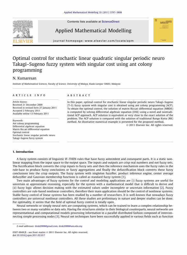
In this approach, ACP is used to obtain a set of expressions. If any expression satisfies fitness function, it will be the optimalsolution of (3). The scheme of computing optimal solution is given in Fig. 3.

According to Boryczka and Wiezorek [29], the following four preparatory steps are essential for a searching process.

Choice of terminals and functionsConstruction of graphDefining fitness functionDefining terminal criteria

3.1. Choice of terminals and functions

A terminal symbol ti 2 T can be a constant or a variable. Every function fi 2 F of a fixed arity can be an arithmetic operator(+,�,⁄, /), an arithmetic function ( sin, cos, exp, log) and an arbitrarily defined function appropriate to the problem underconsideration. The terminal symbols and functions have chosen such that they provided sufficient expressive power to ex-press the solution to a problem. This means that the problem must be solved by a composition of functions and terminalsspecified. For solving the DAE (2), terminal set and function set are taken as T = (0,1,2,3,4,5,6,7,8,9, t) and F = (+, �, ⁄,/, sin,cos, exp, log).

3.2. Construction of graph

In ant colony programming technique, the search space consists of a graph with ‘ nodes where the nodes are the functionsor terminals and edges are weighted by pheromone. An example of such a graph is given in Figs. 4 and 5. Each node in thegraph holds either a function or a terminal. This graph is generated by a randomized process.

3.3. Fitness function

The aim of the fitness function is to provide a basis for competition among available solutions and to obtain the optimalsolution. Hence the fitness function for (3) is defined as

Er ¼ ðk1nðtmÞ � wðkijðtmÞÞÞ2 þXn�1

i;j¼1

ð _kijðtmÞ � /ijðkijðtmÞÞÞ2; ð4Þ

where m represents the equidistance points in the relevant range [0, tf].

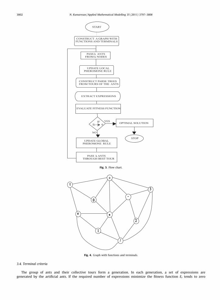
Fig. 3. Flow chart.

Fig. 4. Graph with functions and terminals.


3.4. Terminal criteria

The group of ants and their collective tours form a generation. In each generation, a set of expressions aregenerated by the artificial ants. If the required number of expressions minimize the fitness function Er tends to zero

Fig. 5. Graph with functions and terminals.


or very close to zero and they satisfy the terminal conditions, the process may be stopped; otherwise continue the ACPapproach.

3.5. ACP methodology

Artificial ants build solutions by performing randomized tours on the completely connected graph GðV; EÞ. In the graph,vertices (V) are represented by functions and terminals and the set (E) of edges connect the vertices. The ants move on thegraph by applying a stochastic local decision policy that makes use of pheromone trials and heuristic information. In thisway, ants incrementally build solutions to the given problem.

In the first generation, all edges are initialized by equal pheromone weight. Sent k(<‘) ants through the graph from k start-ing points in a random fashion. Each ant is initially put on a randomly chosen start node. Each ant is moving from the node rto node s in the graph at time t according to the following probability law [38]

prsðtÞ ¼srsðtÞ � ½cs�

bPi2Jk

r½sriðtÞ� � ½ci�

b ;

where cs = (1/(2 + ps))d, ps is the power of symbol s which can be either a terminal symbol or a function, d is the currentlength of the arithmetic expression, b is a parameter which controls the relative weight of the pheromone trail and visibilityand Jk

r is the set of unvisited nodes. The power of the symbols can be calculated from the following Table 1. When an antreaches a node, it determines if the node is a terminal or a function node. If the ant is on a terminal node, the end of the tourhas been reached for that ant.

After having found a tour of an ant, the ant deposits pheromone information on the edges through which it travelled. Itconstitutes a local update of the pheromone trail, which also comprises partial evaporation of the trail. The local update pro-cess is carried out according to the formula:

sijðt þ 1Þ ¼ ð1� qÞ � sijðtÞ þ q � s0;

where (1 � q), q 2 (0,1], is the pheromone decay coefficient, sij is the amount of pheromone trail on edge (i, j) and s0 is theinitial amount of pheromone on edge (i, j).

Each ant has a working memory that stores data about its tour. The ant’s memory is represented programmatically by aparse tree structure. In this tree, the root and branches are functions and leaves are terminals. The depth of the memory treeis limited according to the nature of the problem.

Table 1Power of terminal symbols and functions.

Terminal symbol or function Power

Constant, variable �1Functions 1


The tour e ⁄ t + 1⁄ + 5 of an ant is represented as parse trees in the Fig. 6. The tour e ⁄ t/7⁄ + 4/5 of another ant is repre-sented as parse trees in Fig. 7. The tours of the ants and their corresponding expressions extracted from the parse trees aregiven in Table 2. Some tours of the ants cannot be represented as the parse trees. Such type of tours are given in the followingTable 3. They are discarded when the parse tree construction process is carried out for the tours of the ants. This parse treeconstruction is helpful to converge the solution quickly and also reduces the computation time by discarding the unneces-sary tours. After each generation, a global update of pheromone trail is taken place. The level of pheromone is then changedas follows:

Fig. 6. Parse tree for the tour e ⁄t + 1⁄ + 5.

Fig. 7. Parse tree for the tour e ⁄t /7⁄ + 4/5.

Table 2Tours and expressions.

Tours of ants Expressions

e ⁄ t⁄ et

e ⁄ t + 1⁄ + 5 et+1 + 5e ⁄ t/5⁄ + 0 et/5 + 0e ⁄ t/7⁄ + 4/5 et/7 + 4/5e ⁄ 3 ⁄ t � 2⁄⁄ + 5/2 e3(t�2) + 5/2e ⁄ 3 ⁄ t⁄ + 5/2 � e ⁄ t⁄/7 e3t + 5/2 � et/7

Table 3Discarded tours.

Tours of ants

+e ⁄ t⁄ + 1e ⁄ t + 1⁄ + �5e ⁄ t/ � ⁄2�⁄ e ⁄ t/7⁄ + �/ + 0

Fig. 8. Optimal tour of the ACP.

Fig. 9. Parse tree and its expression.


sijðt þ gÞ ¼ ð1� qÞ � sijðtÞ þ q � 1L;

where g is the number of generations, edges (i, j) belong to the optimal tour found so far and L is the length of this tour. Theaim of the pheromone value update rule is to increase the pheromone values on the solution path. The update rule reducesthe size of the searching region in order to find high quality solution with reasonable computation time. On the updatedgraph, the consecutive cycles of the ant colony algorithm are carried out by sending the ants through the best tour of theprevious generation. The procedure is repeated until the fitness function (4) becomes zero or very close to zero. The optimaltour of the ACP and its corresponding tree are given in Figs. 8 and 9, respectively.

3.6. ACP algorithm

Step 1. Construct a graph with ‘ nodes.Step 2. Initialize the equal weight of pheromone in each edge of the graph.Step 3. Pass k ants through the graph from k starting points and they move to the next node according to the probability

law.Step 4. Apply local update rule after the tour of each ant.Step 5. Construct parse trees from the tours of k ants.Step 6. Extract the expressions from the trees.Step 7. Evaluate the fitness function.Step 8. If Er ? 0 and they satisfy the terminal conditions, then stop. Otherwise apply global update rule.Step 9. Identify the best tour of the previous generation.

Step 10. Pass the same k ants through the best tour and go to Step 4.

4. Numerical example

Consider the optimal control problem:


Minimize

J ¼ E12

xTðtf ÞFTi SFixðtf Þ þ

12

Z tf

0xTðtÞQxðtÞ þ uTðtÞRuðtÞ �

dt�

subject to the stochastic linear singular periodic fuzzy system

FidxðtÞ ¼ AiðtÞxðtÞ þ BiðtÞuðtÞ½ �dt þ DiðtÞuðtÞdWðtÞ; xð0Þ ¼ x0;

where fuzzy term sets T11(0.4158,0.6545), T12(0.597,0.7889), T21(0.3982,0.5249), T12(0.8596,0.6376);

S ¼2 00 0

� �; Fi ¼

1 00 0

� �; A1ðtÞ ¼

�cost 00 �cost

� �; A2ðtÞ ¼

�sint 00 �sint

� �;

BiðtÞ ¼01

� �; R ¼ 0; Q ¼

1 00 0

� �; DiðtÞ ¼

10

� �:

The numerical implementation could be adapted by taking tf = 1 for solving the related MRDE of the above linear singularsystem. The appropriate matrices are substituted in Eq. (2), the MRDE is transformed into DAE in k11 and k12. In this problem,the values of k12 and k22 of the symmetric matrix K(t) are free and let k12 = k22 = 0. Then the optimal control of the system canbe found out by the solution of MRDE.

4.1. Solution obtained using ant colony programming

The graph is generated randomly with 10 nodes. Let q = 0.8 and b = 2. Each edge is initialized by a pheromone weight of1.0. Six ants are taken for sending through the graph from 6 different points. The equidistance points of the interval [0,1] aretaken as m = 0, 0.5, 1.

Table 4Solutions of MRDE.

t ACP solution RK solution

k11 k11

0.0 1.31705803038421 1.317058000000000.1 1.41672486367786 1.416725000000000.2 1.51439669197433 1.514397000000000.3 1.60809844370689 1.608098000000000.4 1.69589471500151 1.695895000000000.5 1.77590910759261 1.775909000000000.6 1.84634297717428 1.846343000000000.7 1.90549340485959 1.905493000000000.8 1.95177021218325 1.951770000000000.9 1.98371184963917 1.983712000000001.0 2.00000000000000 2.00000000000000

Fig. 10. Solution curve for k11.

Fig. 11. Parse tree for k11.


As the ant colony programming is carried out continuously, the solution of each generation will be improved by the pher-omone updating rules. The construction of parse tree for the tour of the ants will converge the optimal solution quickly bydiscarding some unnecessary tours.

After 100 generations, the solutions are obtained from the graph. The numerical solutions of MRDE are calculated anddisplayed in Table 4 using the ACP and RK method. Solution curves by ACP and RK method are given in Fig. 10. Parse treeof ACP is shown in Fig. 11.

Similarly the solution of the above system with the matrix A2 can be found out using ant colony programming.

5. Conclusion

The optimal control for the stochastic linear singular periodic neuro-fuzzy system with singular cost has been found byACP approach. To obtain the optimal control, the solution of MRDE is computed by solving Differential algebraic equation(DAE) using a novel and nontraditional ACP approach. The obtained solution in this method is very close to the exact solutionof the problem. ACP solution is compared with traditional RK solution A numerical example is given to illustrate the derivedresults.

Acknowledgement

The author is very much thankful to the referees for their valuable comments and suggestions to improve this manu-script. The funding of this work by the UMRG grant (Account No: RG099/10AFR) is gratefully acknowledged.

References

[1] L.X. Wang, Stable and optimal fuzzy control of linear systems, IEEE Trans. Fuzzy Syst. 6 (1) (1998) 137–143.[2] L.A. Zadeh, The concept of a linguistic variable and its application to approximate reasoning, Inform. Sci. Part I: (8) (1975) 199–249 (Part II:(8), 301–

357, Part III:(9), 43–80).[3] P. De Wilde, Neural Network Models, Second ed., Springer-Verlag, London, 1997.[4] A. Karakasoglu, S.L. Sudharsanan, M.K. Sundareshan, Identification and decentralized adaptive control using neural networks with application to

robotic manipulators, IEEE Trans. Neural Netw. 4 (1993) 919–930.[5] K.S. Narendra, K. Parathasarathy, Identification and control of dynamical systems using neural networks, IEEE Trans. Neural Netw. 1 (1990) 4–27.[6] J. Jang, Anfis: adaptive-network-based fuzzy inference systems, IEEE Trans. Syst. Man Cybern. 10 (5) (1993) 665–685.[7] Y. Hayashi, J.J. Buckley, Approximations between fuzzy expert systems and neural networks, Int. J. Approx. Reason. 53 (1) (1996) 29–41.[8] X.H. Li, C.L.P. Chen, The equivalence between fuzzy logic systems and feedforward neural networks, IEEE Trans. Neural Netw. 11 (2) (2000) 356–365.[9] J.J. Buckley, Y. Hayashi, Hybrid neural nets can be fuzzy controllers and fuzzy expert systems, Fuzzy Sets Syst. 60 (1993) 135–142.

[10] S.K. Halgamuge, M. Glesner, Neural networks in designing fuzzy systems for real world applications, Fuzzy Sets Syst. 65 (1994) 1–12.[11] S. Mitra, Y. Hayashi, Neuro-fuzzy rule generation: survey in soft computing framework, IEEE Trans. Neural Netw. 2 (3) (2000) 748–768.[12] M. Athens, Special issues on linear quadratic Gaussian problem, IEEE Trans. Automat. Control AC-16 (1971) 527–869.[13] A. Bensoussan, Lecture on stochastic control part I, in: Nonlinear and Stochastic Control, Lecture Notes in Math, vol. 972, Springer-Verlag, Berlin, 1983,

pp. 1–39.[14] F. Bucci, L. Pandolfi, The regulator problem with indefinite quadratic cost for boundary control systems: the finite horizon case, Syst. Control Lett. 39

(2000) 79–86.[15] M.H.A. Davis, Linear Estimation and Stochastic Control, Chapman and Hall, London, 1997.[16] W.M. Wonham, On a matrix Riccati equation of stochastic control, SIAM J. Control Optim. 6 (1968) 681–697.[17] S.P. Chen, X.J. Li, X.Y. Zho, Stochastic linear quadratic regulators with indefinite control weight costs, SIAM J. Control Optim. 36 (5) (1998) 1685–1702.[18] J. Zhu, K. Li, An iterative method for solving stochastic Riccati differential equations for the stochastic LQR problem, Optim. Methods Softw. 18 (2003)

721–732.[19] P. Balasubramaniam, J. Abdul Samath, N. Kumaresan, A. Vincent Antony Kumar, Solution of matrix Riccati differential equation for the linear quadratic

singular system using neural networks, Appl. Math. Comput. 182 (2006) 1832–1839.


[20] P. Balasubramaniam, J. Abdul Samath, N. Kumaresan, Optimal control for nonlinear singular systems with quadratic performance using neuralnetworks, Appl. Math. Comput. 187 (2007) 1535–1543.

[21] P. Balasubramaniam, J. Abdul Samath, N. Kumaresan, A. Vincent Antony Kumar, Neuro approach for solving matrix Riccati differential equation, NeuralParallel Sci. Comput. 15 (2) (2007) 125–135.

[22] C.H. Choi, A survey of numerical methods for solving matrix Riccati differential equation, Proc. Southeastcon (1990) 696–700.[23] S.L. Campbell, Singular Systems of Differential Equations, Pitman, Marshfield MA, 1980.[24] S.L. Campbell, Singular Systems of Differential Equations II, Pitman, Marshfield MA, 1982.[25] F.L. Lewis, A survey of linear singular systems, Circ. Syst. Sig. Proc. 5 (1) (1986) 3–36.[26] G. Da Prato, A. Ichikawa, Quadratic control for linear periodic systems, Appl. Math. Optim. 18 (1988) 39–66.[27] D.G. Luenberger, Dynamic equations in descriptor form, IEEE Trans. Automat. Control 22 (1977) 312–321.[28] R.A. Meyer, C.S. Burrus, A unified analysis of multirate and periodically time-varying digital filters, IEEE Trans. Circ. Syst. 22 (1) (1975) 162–167.[29] M. Boryczka, W. Wiezorek, Solving approximation problems using ant colony programming, Proc. AI-METH (2003) 55–60.[30] E. Wilson, B. Hölldobler, The Ants, Springer-Verlag, 1990.[31] M. Dorigo, V. Maniezzo, A. Colorni, Positive feedback as a search strategy, Technical report politechnico di Milano, Italy, 1991.[32] M. Dorigo, V. Maniezzo, A. Colorni, The ant system: optimization by a colony of cooperating agents, IEEE Trans. Syst. Man Cybern. 26 (1) (1996) 29–41.[33] O. Roux, C. Fonlupt, Ant programming: or how to use ants for automatic programming, Proc. ANTS (2000) 121–129.[34] M. Birattari, G. Di Caro, M. Dorigo, Toward the formal foundatin of Ant programming, in: M. Dorigo, G. Di Caro, M. Sampels (Eds.), Ant Algorithms,

Proceedings of ANTS, 2002, pp. 188–201.[35] N. Kumaresan, P. Balasubramaniam, Singular optimal control for stochastic linear quadratic singular system using ant colony programming, Int. J.

Comput. Math. 87 (14) (2010) 3311–3327.[36] T. Takagi, M. Sugeno, Derivation of fuzzy control rules from human operator’s actions, in: Proceedings of the IFAC Symposium on Fuzzy Information,

Knowledge Representation and Decision Analysis, 1983, pp. 55–60.[37] S.J. Wu, H.H. Chiang, H.T. Lin, T.T. Lee, Neural-network-based optimal fuzzy controller design for nonlinear systems, Fuzzy Sets Syst. 154 (2005) 182–

207.[38] M. Boryczka, Eliminating introns in ant colony programming, Fund. Inform. 68 (2005) 1–19.

applied mathematical modelling - university of malaya · optimal control for stochastic linear...

Documents