applied mathematical modelling - dl.edi-info.ir queue with working vacations, vacation... ·...

Applied Mathematical Modelling 37 (2013) 3879–3893

Contents lists available at SciVerse ScienceDirect

Applied Mathematical Modelling

journal homepage: www.elsevier .com/locate /apm

MAP/PH/1 queue with working vacations, vacation interruptionsand N policy

C. Sreenivasan a, Srinivas R. Chakravarthy b, A. Krishnamoorthy c,⇑a Department of Mathematics, Government College, Chittur, Palakkad 678104, Indiab Department of Industrial Manufacturing Engineering, Kettering University, Flint, MI 48504, USAc Department of Mathematics, Cochin University of Science and Technology, Cochin 682022, India

a r t i c l e i n f o

Article history:Received 27 September 2011Received in revised form 1 June 2012Accepted 5 July 2012Available online 1 September 2012

Keywords:Working vacationVacation interruptionMarkovPhase type distributionAlgorithmic probability

0307-904X/$ - see front matter � 2012 Elsevier Inchttp://dx.doi.org/10.1016/j.apm.2012.07.054

⇑ Corresponding author. Tel.: +91 484 2577447.E-mail addresses: [email protected]

moorthy).

a b s t r a c t

In this paper we study a MAP/PH/1 queueing model in which the server is subject to takingvacations and offering services at a lower rate during those times. The service is returned tonormal rate whenever the vacation gets over or when the queue length hits a specificthreshold value. This model is analyzed in steady state using matrix analytic methods.An illustrative numerical example is discussed.

� 2012 Elsevier Inc. All rights reserved.

1. Introduction

Queues with vacations have been extensively studied by several authors. We refer the reader to the paper by Doshi [1] forearlier works (prior to 1985) on vacation models and to the book by Tian and Zhang [2] for works through 2006. Queueingmodels with vacations under different scenarios such as (a) exhaustive clearance where the server clears all the work in thesystem before going on a vacation and returns to work only after completing the current vacation; (b) limited clearance inwhich the server proceeds on a vacation after completing a fixed number of services or after a fixed period of time; and (c)gated clearance in which the server returning from a vacation serves only those who are waiting at that instant before goingon another vacation. The server can take single or multiple vacations at a time. For example, in the case of single vacation theserver remains in the system even if there is no one waiting, whereas in the multiple vacations the server will start anothervacation when the system is empty whenever coming back from a vacation.

Servi and Finn [3] introduced a working vacation model with the idea of offering services but at a lower rate whenever theserver is on vacation. Their model was generalized to the case of M/G/1 in ([4,5]), and to GI/M/1 model in [6]. A survey ofworking vacation models with emphasis on the use of matrix analytic methods is given in Tian et al. [7]. Working vacationmodels have a number of applications in practice. Two such examples are given in [7].

Recently, Li and Tian [8] studied an M=M=1 queue with working vacations in which vacationing server offers services at alower rate for the first customer arriving during a vacation. Upon completion of the service at a lower rate the server will (a)continue the current vacation (if not finished) or take another vacation (if the working vacation expired) if there are no

. All rights reserved.

(C. Sreenivasan), [email protected] (S.R. Chakravarthy), [email protected] (A. Krishna-

http://dx.doi.org/10.1016/j.apm.2012.07.054

mailto:[email protected]



http://dx.doi.org/10.1016/j.apm.2012.07.054

http://www.sciencedirect.com/science/journal/0307904X

http://www.elsevier.com/locate/apm

3880 C. Sreenivasan et al. / Applied Mathematical Modelling 37 (2013) 3879–3893

customers waiting or (b) resume at a normal rate (irrespective of whether the vacation expired or not) if there are customerswaiting. Resuming services at a normal rate while the vacation is still in progress corresponds to the vacation beinginterrupted.

Very recently, Zhang and Hou [9] studied a MAP=G=1 queue with working vacations and vacation interruption using sup-plementary variable method. In this model, the authors assume that the vacation times are exponentially distributed andthat the server gets back to normal service mode when at the service (offered during a vacation) completion the systemhas at least one customer waiting in the queue. The server is allowed to take multiple vacations. In this paper we extendthe work of [8] in the following way. First we assume a more versatile point process to model the arrivals. Secondly, weuse phase type services which generalizes some of the well-known distributions such as exponential, generalized Erlang,and hyperexponential. Thirdly, we introduce a threshold, say, 1 6 N <1, such that the server offering services (at a lowerrate) during a vacation will have the vacation interrupted, the moment the queue size hits N.

In this paper, we consider a single server queueing model in which customers arrive according to a versatile point process,namely, Markovian arrival process (MAP). A MAP is a tractable class of Markov renewal processes. It should be noted that byappropriately choosing the parameters of the MAP the underlying arrival process can be made as a renewal process. The MAPis a rich class of point processes that includes many well-known processes such as Poisson, PH-renewal processes, and Mar-kov-modulated Poisson process. One of the most significant features of the MAP is the underlying Markovian structure andfits ideally in the context of matrix-analytic solutions to stochastic models. Matrix-analytic methods were first introducedand studied by Neuts [10]. As is well known, Poisson processes are the simplest and most tractable ones used extensivelyin stochastic modelling. The idea of the MAP is to significantly generalize the Poisson processes and still keep the tractabilityfor modelling purposes. Furthermore, in many practical applications, notably in communications engineering, productionand manufacturing engineering, the arrivals do not usually form a renewal process. So, MAP is a convenient tool to modelboth renewal and non-renewal arrivals. While MAP is defined for both discrete and continuous times, here we will need onlythe continuous time case.

The MAP in continuous time is described as follows. Let the underlying Markov chain be irreducible and let Q � be the gen-erator of this Markov chain. At the end of a sojourn time in state i, that is exponentially distributed with parameter ki, one ofthe following two events could occur: with probability pijð1Þ the transition corresponds to an arrival and the underlying Mar-kov chain is in state j with 1 6 i; j 6 m; with probability pijð0Þ the transition corresponds to no arrival and the state of theMarkov chain is j, j – i. Note that the Markov chain can go from state i to state i only through an arrival. Define matricesD0 ¼ ðd0

ijÞ and D1 ¼ ðd1ijÞ such that d0

ii ¼ �ki, 1 6 i 6 m, d0ij ¼ kipijð0Þ, for j – i and d1

ij ¼ kipijð1Þ, 1 6 i; j 6 m. By assuming D0

to be a nonsingular matrix, the interarrival times will be finite with probability one and the arrival process does not termi-nate. Hence, we see that D0 is a stable matrix. The generator Q � is then given by Q � ¼ D0 þ D1.

Thus, D0 governs the transitions corresponding to no arrival and D1 governs those corresponding to an arrival. It can beshown that MAP is equivalent to Neuts’ versatile Markovian point process. The point process described by the MAP is a spe-cial class of semi-Markov processes with transition probability matrix given by
Z x
0eD0t dtD1 ¼ ½I � eD0x�ð�D0Þ�1D1; x P 0:

For use in sequel, let eðrÞ, ejðrÞ and Ir denote, respectively, the (column) vector of dimension r consisting of 1’s, columnvector of dimension r with 1 in the jth position and 0 elsewhere, and an identity matrix of dimension r. When there is noneed to emphasize the dimension of these vectors we will suppress the suffix. Thus, e will denote a column vector of 1’sof appropriate dimension. The notation �will stand for the Kronecker product of two matrices. Thus, if A is a matrix of orderm� n and B is a matrix of order p� q, then A� B will denote a matrix of order mp� nq, whose (i, j)th block matrix is given byaijB. For more details on Kronecker products and sums, we refer the reader to [11].

Let p be the stationary probability vector of the Markov process with generator Q �. That is, p is the unique (positive) prob-ability vector satisfying.

pQ � ¼ 0; pe ¼ 1: ð1Þ

Let n be the initial probability vector of the underlying Markov chain governing the MAP. Then, by choosing n appropri-ately we can model the time origin to be (a) an arbitrary arrival point; (b) the end of an interval during which there are atleast k arrivals; and (c) the point at which the system is in specific state such as the busy period ends or busy period begins.The most interesting case is the one where we get the stationary version of the MAP by n = p. The constant k ¼ pD1e, referredto as the fundamental rate gives the expected number of arrivals per unit of time in the stationary version of the MAP.

Often, in model comparisons, it is convenient to select the time scale of the MAP so that k has a certain value. That isaccomplished, in the continuous MAP case, by multiplying the coefficient matrices D0 and D1, by the appropriate commonconstant. For further details on MAP and their usefulness in stochastic modelling, we refer to [12–14] and for a reviewand recent work on MAP we refer the reader to [15,16].

This paper is organized as follows. In Section 2 we provide a description of the queueing model under study. In Section 3the steady state analysis of the model is presented. In Section 4 we discuss an illustrative numerical example.

C. Sreenivasan et al. / Applied Mathematical Modelling 37 (2013) 3879–3893 3881

2. Mathematical model

We consider a single server queueing system in which customers arrive according to a Markovian arrival process withparameter matrices D0 and D1 of dimension m. An arriving primary customer finding the server free (i.e., on vacation) getsinto service immediately but at a lower rate. On the other hand an arriving customer finding the server busy gets into a buf-fer (of infinite capacity) for the server to become available. The service times follow a phase type distribution with represen-tation (a,T) of order n. When the system becomes empty at the time of a completion of a service, the server will go on avacation. The duration of a vacation is assumed to be exponentially distributed with parameter g. A vacation is interruptedwhen a customer arrives during that time. However, the server offers services to those customers arriving during a vacationat a lower rate as compared to the other (regular) customers. We assume that the service times of those customers (served ata lower rate) are also of phase type but with representation (a,hT), with 0 < h < 1. The server continues to serve at this rateuntil either the vacation expires or the queue length hits a pre-determined threshold, say, N, 1 6 N <1. At this instant, theserver instantaneously switches over to the normal rate and continues to serve at this rate until the system becomes empty.At the end of a vacation if there is no customer waiting for service, the server takes another vacation. Let l denote the regularservice rate. It is easy to verify that l ¼ ½að�TÞ�1e��1 and the vacation mode of service has rate hl.

3. steady-state analysis

In this section we will discuss the steady-state analysis of the model under study.

3.1. The QBD process

The model described in Section 2 can be studied as a quasi-birth-and-death (QBD) process. First, we set up necessarynotations. Define NðtÞ to be the number of customers in the system at time t,

S1ðtÞ ¼0; if the service is in vacation mode;1; if the service is normal;

�
S2ðtÞ, the phase of the service process when the server is busy, and MðtÞ to be the phase of the arrival process at time t. It iseasy to verify that fðNðtÞ; S1ðtÞ; S2ðtÞ;MðtÞÞ : t P 0g is a quasi-birth-and-death process (QBD) with state space
X ¼[1i¼0

lðiÞ;

where

lð0Þ ¼ fð0;1Þ; ð0;2Þ; . . . ð0;mÞg;

and for i P 1,

lðiÞ ¼ fði; j1; j2; kÞ : j1 ¼ 0 or 1;1 6 j2 6 n;1 6 k 6 mg:

Note that when NðtÞ ¼ 0, S1ðtÞ and S2ðtÞ do not play any role and will not be tracked. In this case only the state, MðtÞ, of thearrival process needs to be accounted.

The generator, Q, of the QBD process under consideration is of the form

Q ¼

D0 C0

C2 B1 I � D1

. .. . .

. . ..

B2 B1 I � D1

B2 B1 e� I � D1

e02ð2Þ � T0a� I A1 A0

A2 A1 A0

. .. . .

. . ..

0BBBBBBBBBBBB@

1CCCCCCCCCCCCA; ð2Þ

where the (block) matrices appearing in Q are as follows.

C0 ¼ ½a� D1 O�; C2 ¼ hT0 � IT0 � I

� �;

B1 ¼hT � D0 � gI gI

O T � D0

� �; B2 ¼

hT0a� I O

O T0a� I

" #;

A0 ¼ I � D1; A1 ¼ T � D0; A2 ¼ T0a� I: ð3Þ


3.2. The steady-state probability vector

Defining A ¼ A0 þ A1 þ A2 and d to be the steady-state probability vector of the irreducible matrix A, it is easy to verify thatthe vector d satisfying

dA ¼ 0; de ¼ 1; ð4Þ

is given by

d ¼ ðlað�TÞ�1 � pÞ; ð5Þ

where p as given in (1).The condition dA0e < dA2e required for the stability of the queueing model under study (see [10]) reduces to k < l.Let x be the steady-state probability vector of Q . Partition this vector as:

x ¼ ðx0; x1; x2 . . . ; . . . ; xN ; xNþ1; . . .Þ;

where x0 is of dimension m, x1; x2; . . . ; xN are of dimension 2mn and xNþ1; xNþ2; . . . are of dimension mn.Under the condition that k < l, the steady-state probability vector x is obtained (see, e.g. [10]) as follows:

xNþi ¼ xNþ1Ri�1; i P 1; ð6Þ

where the matrix R is the minimal nonnegative solution to the matrix quadratic equation:

R2A2 þ RA1 þ A0 ¼ 0; ð7Þ

and the vectors x0; . . . ; xNþ1 are obtained by solving

x0D0 þ x1C2 ¼ 0;x0C0 þ x1B1 þ x2B2 ¼ 0;xi�1ðI � D1Þ þ xiB1 þ xiþ1B2 ¼ 0; 2 6 i 6 N � 1;

xN�1ðI � D1Þ þ xNB1 þ xNþ1ðe02ð2Þ � T0a� IÞ ¼ 0;xNðe� I � D1Þ þ xNþ1ðA1 þ RA2Þ ¼ 0;

ð8Þ

subject to the normalizing condition
XN
i¼0

xieþ xNþ1ðI � RÞ�1e ¼ 1: ð9Þ

The computation of the R matrix can be carried out using a number of well-known methods such as logarithmic reduc-tion. We will list only the main steps involved in the logarithmic reduction algorithm for the computation of R. For full detailsof the logarithmic reduction algorithm we refer the reader to [17].

Logarithmic Reduction Algorithm for R:Step 0: H ð�A1Þ�1A0, L ð�A1Þ�1A2, G ¼ L, and T ¼ H.Step 1:

U ¼ HLþ LHM ¼ H2

H ðI � UÞ�1M

M L2

L ðI � UÞ�1M

G Gþ TL

T TH

Continue Step 1 until jje� Gejj1 < �.Step 2: R ¼ �A0ðA1 þ A0GÞ�1.The computation of the vectors x0; . . . ; xNþ1 can be carried out by exploiting the special structure of the coefficient matri-

ces and the details are omitted. For use in the sequel, we partition xi ¼ ðui; v iÞ; 1 6 i 6 N, where ui and v i are of dimensionmn.

3.3. The stationary waiting time distribution in the queue

The stationary waiting time distribution in the queue of a customer is derived here. We obtain this by conditioning on thefact that at an arrival epoch the server is serving in normal mode or in vacation mode. First note that an arriving customerwill enter into service immediately (at a lower service rate) when the server is on vacation. Otherwise, the customer has towait before getting into service (either at a lower rate or normal rate).


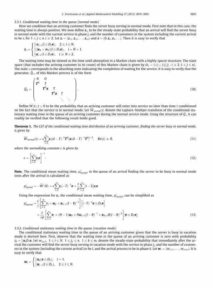
3.3.1. Conditional waiting time in the queue (normal mode)Here we condition that an arriving customer finds the server busy serving in normal mode. First note that in this case, the

waiting time is always positive. We now define zi;j to be the steady-state probability that an arrival will find the server busyin normal mode with the current service in phase j, and the number of customers in the system including the current arrivalto be i, for 1 6 j 6 n; i P 2. Let zi ¼ ðzi;1; zi;2; . . . ; zi;nÞ and z ¼ ð0; z2; z3; . . .Þ. Then it is easy to verify that

zi ¼

1k v i�1ðI � D1eÞ; 2 6 i 6 N;1k ðuN þ vNÞðI � D1eÞ; i ¼ N þ 1;1k xi�1ðI � D1eÞ; i P N þ 2:

8><>:
The waiting time may be viewed as the time until absorption in a Markov chain with a highly sparse structure. The state
space (that includes the arriving customer in its count) of this Markov chain is given by X1 ¼ f�g [ fði; jÞ : i P 2;1 6 j 6 ng.The state ⁄ corresponds to the absorbing state indicating the completion of waiting for the service. It is easy to verify that thegenerator, eQ 1, of this Markov process is of the form

~Q 1 ¼

0 O

T0 T

T0a T

T0a T

. .. . .

.

0BBBBBB@

1CCCCCCA: ð10Þ

Define WðtÞ; t > 0 to be the probability that an arriving customer will enter into service no later than time t conditionedon the fact that the service is in normal mode. Let fW normalðsÞ denote the Laplace–Stieltjes transform of the conditional sta-tionary waiting time in the queue of an arriving customer during the normal service mode. Using the structure of ~Q1 it canreadily be verified that the following result holds good.

Theorem 1. The LST of the conditional waiting time distribution of an arriving customer, finding the server busy in normal mode,is given by

fW normalðsÞ ¼ cX1i¼2

ziðsI � TÞ�1T0½aðsI � TÞ�1T0�i�2; ReðsÞP 0; ð11Þ

where the normalizing constant c is given by

c ¼X1i¼2

zie

" #�1

: ð12Þ

Note. The conditional mean waiting time, l0normal, in the queue of an arrival finding the server to be busy in normal modesoon after the arrival is calculated as

l0normal ¼ �fW 0ð0Þ ¼ cX1i¼2

zið�TÞ�1eþ clX1i¼2

ði� 2Þzie:

Using the expression for zi, the conditional mean waiting time, l0normal, can be simplified as

l0normal ¼ck

XN

i¼1

v i þ uN þ xNþ1ðI � RÞ�1

" #ð�TÞ�1e� D1eh i

þ ckl

X1i¼1

v i þ ðN � 1ÞuN þ NxNþ1ðI � RÞ�1 þ xNþ1RðI � RÞ�2

" #½e� D1e�: ð13Þ

3.3.2. Conditional stationary waiting time in the queue (vacation mode)The conditional stationary waiting time in the queue of an arriving customer given that the server is busy in vacation

mode is derived here. First, observe that the waiting time in the queue of an arriving customer is zero with probabilityz0 ¼ 1

k x0D1e. Let wi;j2 ;k; 1 6 i 6 N; 1 6 j2 6 n; 1 6 k 6 m, denote the steady-state probability that immediately after the ar-rival the customer will find the server busy serving in vacation mode with the service in phase j2 and the number of custom-ers in the system (including the current arrival) to be i, and the arrival process to be in phase k. Let wi ¼ ðwi;1;1; . . . ;wi;n;mÞ. It iseasy to verify that

wi ¼1k x0ða� D1Þ; i ¼ 1;1k ui�1ðI � D1Þ; 2 6 i 6 N:

(


Observe that the conditional waiting time in the queue of an arriving customer finding the server busy in vacation modesoon after the arrival depends on the future arrivals due to the threshold placed on the system for bringing back the servicerate to normal. Thus, we need to keep track of the phase of the arrival process up until the service rate becomes normal dueeither to meeting the threshold or the vacation expiring. Towards this end, we define the following set of states.

Let ði; j; j2; kÞ; 1 6 i 6 N � 1; 1 6 j 6 i; 1 6 j2 6 n; 1 6 k 6 m, denote the state that corresponds to the server being invacation mode with i customers in the queue; the arriving customer’s position in the queue is j; the current service is in phasej2, and the arrival process is in phase k. Define ði�; j2Þ : 1 6 i� 6 N � 1;1 6 j2 6 n to be the state that corresponds to the serverserving in normal mode and the position of the tagged customer in the queue being i� and the current service in phase j2.

Let i = fði; j; j2; kÞ;1 6 j 6 i;1 6 j2 6 n;1 6 k 6 mg; 1 6 i 6 N � 1, and i� = fði�; j2Þ;1 6 j2 6 ng; 1 6 i� 6 N � 1.Before we formally state the result we need the following notations. Define:

� Ir is an identity matrix of dimension r.

� bIr is a matrix of dimension r � N � 1 of the form

Ir ¼ Ir 0ð Þ; 1 6 r 6 N � 1:

� �Ir is a matrix of dimension r � r � 1 of the form

�Ir ¼0

Ir�1

� �; 2 6 r 6 N � 1:

� eIr is a matrix of dimension r � r þ 1 of the form
eIr ¼ Ir 0ð Þ; 1 6 r 6 N � 2:
Let

L1;1 ¼

T

T0a T

T0a T

. .. . .

.

T0a T

0BBBBBBBBBB@

1CCCCCCCCCCA; L2;1 ¼

gbI1 � I � e

gbI2 � I � e

..

.

gbIN�2 � I � e

IN�1 � ðgI � eþ I � D1eÞ

0BBBBBBBBBBBB@

1CCCCCCCCCCCCA; ð14Þ

L2;2 ¼

eB1eI1 � I � D1

h�I2 � T0a� I I2 � eB1eI2 � I � D1

h�I3 � T0a� I I3 � eB1eI3 � I � D1

. .. . .

.

h�IN�1 � T0a� I IN�1 � eB1

0BBBBBBB@

1CCCCCCCA; ð15Þ

and
eB1 ¼ ðhT � D0Þ � gI: ð16Þ
Under this setup, one can readily verify the following result.

Theorem 2. The conditional waiting time distribution in the queue of an arriving customer finding the server in vacation modesoon after the arrival is of phase type with representation ðc; LÞ of order ½ðN � 1Þnþ 0:5NðN � 1Þmn�, where

c ¼ dð0;w2; e02ð2Þ �w3; e03ð3Þ �w4; ; e0N�1ðN � 1Þ �wNÞ; ð17Þ

and

L ¼L1;1 0L2;1 L2;2

� �; ð18Þ

where the normalizing constant is given by d ¼PN

i¼1wieh i�1

:

Note. The conditional mean waiting time, l0vacation, in the queue of an arrival finding the server to be busy during vacationmode soon after the arrival is calculated as l0vacation ¼ cð�LÞ�1e. The computation of this mean is achieved by exploiting thespecial structure of c and L. We will briefly present the steps involved in this.


Defining

cð�LÞ�1 ¼ ða;bÞ;

and partitioning the vectors a and b as

a ¼ ða1; ;aN�1Þ;

b ¼ ðb1;1;b2;1;b2;2; . . . ;bN�1;1; . . . ;bN�1;N�1Þ;

where ai; 1 6 i 6 N � 1, is of dimension n and bi;j; 1 6 j 6 i; 1 6 i 6 N � 1, is of dimension of mn, the mean l0vacation is givenby

l0vacation ¼XN�1

i¼1

aieþXi

j¼1

bi;je

" #:

The vectors ai;1 6 i 6 N � 1; and bi;j; 1 6 j 6 i; 1 6 i 6 N � 1, are ideally suited for solving using any of the well-knownmethods such as (block) Gauss–Seidel. The necessary equations are as follows:

a1 ¼ a2T0að�TÞ�1 þ gXN�1

r¼1

br;1ð�T�1 � eÞ þ bN�1;1ð�T�1 � D1eÞ;

ai ¼ aiþ1T0að�TÞ�1 þ gXN�1

r¼i

br;ið�T�1 � eÞ þ bN�1;ið�T�1 � D1eÞ; 2 6 i 6 N � 2;

aN�1 ¼ gbN�1;N�1ð�T�1 � eÞ þ bN�1;N�1ð�T�1 � D1eÞ;

b1;1 ¼ ½w2 þ hb2;2ðT0a� IÞ�ð�eB1Þ�1;

bi;1 ¼ ½bi�1;1ðI � D1Þ þ hbiþ1;2ðT0a� IÞ�ð�eB1Þ�1; 2 6 i 6 N � 2;

bi;j ¼ ½bi�1;jðI � D1Þ þ hbiþ1;jþ1ðT0a� IÞ�ð�eB1Þ�1; 2 6 j 6 i� 1; 3 6 i 6 N � 2;

bi;i ¼ ½wiþ1 þ hbiþ1;iþ1ðT0a� IÞ�ð�eB1Þ�1; 2 6 i 6 N � 2;

bN�1;j ¼ bN�2;jðI � D1Þð�eB1Þ�1; 1 6 j 6 N � 2;

bN�1;N�1 ¼ wNð�eB1Þ�1;

subject to the condition

a1T0 þ hXN�1

i¼1

bi;1ðT0 � eÞ ¼ 1� dw1e:

3.3.3. The stationary waiting time in the queueFrom the knowledge of conditional stationary waiting time in the queue, one can get the (unconditional) stationary wait-

ing time in the queue and the details are omitted.

Note. The (unconditional) mean, l0WTQ , waiting time of a customer in the queue is obtained as

l0WTQ ¼1k

XN

i¼1

v i þ uN þ xNþ1ðI � RÞ�1

" #½ð�TÞ�1e� D1e�

þ 1kl

X1i¼1

v i þ ðN � 1ÞuN þ NxNþ1ðI � RÞ�1 þ xNþ1RðI � RÞ�2

" #½e� D1e� þ 1

d

XN�1

i¼1

aieþXi

j¼1

bi;je

" #: ð19Þ

3.4. Analysis of slow service mode

In this section we will discuss the duration of the server spending in slow service mode as well as the number of visits tolevel 0 before hitting normal service mode.

3.4.1. The duration in slow service modeThe duration, Tslow, in slow service mode is defined as the time the server starts in slow service mode (through initiating a

working vacation) until either the server takes another vacation or the server gets back to normal mode through the working


vacation expiring. In this section we will show that the random variable Tslow can be studied as the time until absorption in afinite state continuous time Markov chain with two absorbing states. We first define

cM ¼ c1ða� x0D1;0Þ;

M ¼

eB1 I � D1

hðT0a� IÞ eB1 I � D1

hðT0a� IÞ eB1 I � D1

. .. . .

.

hðT0a� IÞ eB1

0BBBBBBBBBBBB@

1CCCCCCCCCCCCA;

M01 ¼

hðT0 � eÞ0...

0

0BBBB@1CCCCA; M0

2 ¼

gege

..

.

gegeþ ðe� D1eÞ

0BBBBBBB@

1CCCCCCCA;

where c1 ¼ ½x0D1e��1 is the normalizing constant and eB1 is as given in (16). The matrix M is of dimension Nmn. First note thatthe probability, pslow, that the server will serve only in slow mode before taking another vacation is given bypslow ¼ cMð�MÞ�1M0

1. We now have the following result.

Theorem 3. The (conditional) probability density function of Tslow, conditioned on the fact that the slow service mode endsthrough the server taking another vacation, is given by

fTslowðyÞ ¼ 1

pslowcMeMyM0

1; y P 0: ð20Þ

Given that the slow service mode ends through the server taking another vacation, the (conditional) mean time spent inslow mode can be calculated as

l0SM ¼1

pslowcMð�MÞ�2M0

1: ð21Þ

Note. 1. The special structure of cM; M, and M01 is to be exploited when computing this mean. The details are similar to the

computation of l0vacation and hence omitted.2. By a similar argument we can get the (conditional) probability density function of Tslow and the conditional mean,

conditioned on the fact that the server ends the slow service mode by entering into the normal rate. The details are omitted.

3.4.2. The distribution of the number of visits to level 0 before hitting normal service modeWe consider the queueing system at an arrival epoch that finds the server in vacation mode. At this instant the service

will start in slow mode. The quantity that is of interest here is the probability mass function, fpk; k P 0g, of the number ofvisits to level 0 before hitting normal service mode. This mass function and its associated measures such as mean and stan-dard deviation, play an important role in the qualitative study of the model under consideration. Using the set up in 3.4.1 itcan easily be verified that

pk ¼ cMð�MÞ�1BkM02; k P 0; ð22Þ

where

B ¼ h ðe1e01 � T0a� ð�D0Þ�1D1Þh i

ð�MÞ�1: ð23Þ

Note. It is easy to see that the mean number of visits, lNVZ , to level 0 before hitting level N þ 1 is obtained as

lNVZ ¼ cMð�MÞ�1BðI � BÞ�2M02: ð24Þ

The computation of lNVZ can be carried out by exploiting the special structure of cM; M, and B. Below, we will outline onlythe main steps. Towards this end, we first define

cMð�MÞ�1 ¼ ðd1; . . . ;dNÞ;


where the vectors di; 1 6 i 6 N, are of dimension nm, and their computation is very similar to the one discussed in findingl0vacation. From Eq. (23) it is clear that B is of the form

B ¼

B1 B2 BN

0 0 0

..

. ... ..

.

0 0 0

0BBBBBBB@

1CCCCCCCA;

where the matrices Bi; 1 6 i 6 N, of order nm are obtained by solving the following equations that are ideally suited for anyof the well-known methods such as (block) Gauss–Seidel.

B1 ¼ h½B2ðT0a� IÞ þ ðT0a� ð�D0Þ�1D1Þ�ð�eB1Þ�1;

Bi ¼ ½Bi�1ðI � D1Þ þ hBiþ1ðT0a� IÞ�ð�eB1Þ�1; 2 6 i 6 N � 1;

BN ¼ BN�1ðI � D1Þð�eB1Þ�1;

subject to the condition

hB1ðT0 � eÞ þ BNðe� D1eÞ þ gXN

i¼1

Bie ¼ hðT0 � eÞ;

and eB1 is as given in (16).Using the facts that

pslow ¼ hd1ðT0 � eÞ and lNVZ ¼ cMð�MÞ�1ðI � BÞ�2M 02 � 1;

and the special form of B, it can easily be verified that

lNVZ ¼ hd1ðI � B1Þ�1ðT0 � eÞ:

3.4.3. The uninterrupted vacation timeThe uninterrupted vacation time is defined as the duration that begins with the server becoming idle (and thus starts a

vacation) until a new arrival interrupts the vacation. It is easy to verify that this duration is of phase type with representationðn;D0Þ of dimension m, where n ¼ c2ðhu1 þ v1ÞðT0 � IÞ and c2 is the normalizing constant given by c2 ¼ ½ðhu1 þ v1ÞðT0 � eÞ��1.The mean, lUIV , is calculated as lUIV ¼ nð�D0Þ�1e.

3.5. Key system performance measures

In this section we list a number of key system performance measures to bring out the qualitative aspects of the modelunder study. Note that these are in addition to the ones such as the conditional mean waiting times and mean waiting timelisted above. The measures are listed below along with their formulae for computation:

1. The probability that the system is idle: PIDLE ¼ x0e.2. The probability that the server is serving at a lower rate: PLR ¼

PNi¼1uie.

3. The probability that the server is serving at a normal rate rate: PNR ¼PN

i¼1v ieþ xNþ1ðI � RÞ�1e.4. The mean number of customers in the system: lNS ¼

PNi¼1iðui þ v iÞeþ NxNþ1ðI � RÞ�1eþ xNþ1ðI � RÞ�2e.

4. Numerical results

In order to bring out the qualitative nature of the model under study, we present a few representative examples in thissection. For the arrival process we consider the following five sets of matrices for D0 and D1:

1. Erlang (ERA)

D0 ¼

�5 5�5 5

�5 5�5 5

�5

0BBBBBB@

1CCCCCCA D1 ¼

5

0BBBBBB@

1CCCCCCA


2. Exponential (EXA)

D0 ¼ ð�1Þ; D1 ¼ ð1Þ

3. Hyperexponential (HEA)

D0 ¼�10 0

0 �1

� �; D1 ¼

9 10:9 0:1

� �
4. MAP with negative correlation ðMNAÞ
D0 ¼�2 2 00 �2 00 0 �450:5

0B@1CA; D1 ¼

0 0 00:02 0 1:98

445:995 0 4:505

0B@1CA

5. MAP with positive correlation ðMPAÞ

D0 ¼�2 �2 00 �2 00 0 �450:5

0B@1CA; D1 ¼

0 0 01:98 0 0:02

4:505 0 445:995

0B@1CA:

0.0

0.5

1.0

1.5

2.0

510152025

510

1520 η

N

(a) Erlang arrivals

0.0

0.5

1.0

1.5

2.0

510152025

510

1520 η

N

(e) MAP with positive correlation arrivals

0.0

0.5

1.0

1.5

2.0

510152025

510

1520 η

N

(b) Exponential arrivals

0.0

0.5

1.0

1.5

2.0

510152025

5101520 η

N

(c) Hyperexponential arrivals

0.0

0.5

1.0

1.5

2.0

510152025

510

1520 η

N

(d) MAP with negative correlation arrivals

λ = 1, μ = 1.1, θ= 0.6

Fig. 1. Mean duration in slow mode – Erlang services.


All these five MAP processes are normalized so as to have an arrival rate of 1. However, these are qualitatively different inthat they have different variance and correlation structure. The first three arrival processes, namely ERA, EXA, and HEA, cor-respond to renewal processes and so the correlation is 0. The arrival process labelled MNA has correlated arrivals with cor-relation between two successive inter-arrival times given by �0.4889 and the arrival process corresponding to the onelabelled MPA has a positive correlation with value 0.4889. The ratio of the standard deviations of the inter-arrival timesof these five arrival processes with respect to ERA are, respectively, 1, 2.2361, 5.0194, 3.1518, and 3.1518.

For the service time distribution we consider the following two phase type distributions.

1. Erlang (ERS)

a ¼ ð1;0Þ; T ¼�2 20 �2

� �
2. Hyperexponential (HES)
a ¼ ð0:9;0:1Þ; T ¼�1:90 0

0 �0:19

� �

These above two distributions will be normalized to have a specific mean in our illustrative example. Note that these arequalitatively different in that they have different variances. The ratio of the standard deviation of HES to that of ERS is 3.1745.

0.0

0.5

1.0

1.5

2.0

510152025

510

1520 η

N

(a) Erlang arrivals

0.0

0.5

1.0

1.5

2.0

510152025

510

1520 η

N


0.0

0.5

1.0

1.5

2.0

510152025

510

1520 η

N


0.0

0.5

1.0

1.5

2.0

510152025

510

1520 η

N


0.0

0.5

1.0

1.5

2.0

510152025

510

1520 η

N


λ = 1, μ = 1.1, θ= 0.6

Fig. 2. Mean duration in slow mode – hyperexponential services.

0.00.20.40.60.81.01.21.41.61.8

510152025

510

1520 η

N

(a) Erlang arrivals

0.00.20.40.60.81.01.21.41.61.8

510152025

510

1520 η

N


0.00.20.40.60.81.01.21.41.61.8

510152025

510

1520 η

N


0.00.20.40.60.81.01.21.41.61.8

510152025

510

15

η

N


0.00.20.40.60.81.01.21.41.61.8

510152025

510

1520 η

N


λ = 1, μ = 1.1, θ= 0.6

Fig. 3. Mean number of visits to level zero – Erlang services.


Illustrative example: The purpose of this example is to see how various system performance measure behave under dif-ferent scenarios. We fix k ¼ 1; l ¼ 1:1, and h ¼ 0:6. First we look at the effect of varying N and g on the performance mea-sures: (conditional) mean duration of service in slow mode which ends in the server taking another vacation and the meannumber of visits to level zero before hitting the normal service mode. Due to space restriction, we will display only a fewfigures and others are available upon request from the authors. In the following we summarize the observations based onvarious graphs of these performance measures.

� An increase in g leads to a decrease in the mean duration of vacation. Hence a switch from the lower service rate to thenormal one occurs more frequently. Once the service rate is brought back to normal, the server clears out the customers ata faster rate. So the measure, Pidle, appears to increase as g increases. This is true for all values of N and for all combinationsof arrival and service processes under study. As N increases the duration of vacation mode of service gets extended, as isexpected. Due to the slow service rate the customers get accumulated faster. So Pidle decreases until the service rate getsto normal. Also note that the probability, PLR, that the server is serving at a low rate increases as N is increased (for fixed g)for all combinations of arrival and service times. This in turn will cause the probability, PNR, of the server serving undernormal mode to decrease as N increases. As expected, the measure PNR appears to increase with increasing g. When com-paring the mean duration of service in slow mode (see Figs. 1 and 2), we notice (for fixed N and g) that HES services yield alower value as opposed to ERS services. This is the case for all five arrival processes considered.� Referring to Figs. 3 and 4, we note that as g increases, the measure lNVZ appears to decrease in all cases, as expected,

for any fixed N. Among renewal arrivals,those with larger variation yields a smaller value for this measure. That is,HEA has a smaller value compared to EXA and EXA has a smaller value compared to ERA. Among correlated arrivals,

0.00.20.40.60.81.01.21.41.61.8

510152025

510

1520 η

N

(a) Erlang arrivals

0.00.20.40.60.81.01.21.41.61.8

510152025

510

1520 η

N


0.00.20.40.60.81.01.21.41.61.8

510152025

510

1520 η

N


0.00.20.40.60.81.01.21.41.61.8

510152025

510

1520 η

N


0.00.20.40.60.81.01.21.41.61.8

510152025

510

1520 η

N


λ = 1, μ = 1.1, θ= 0.6

Fig. 4. Mean number of visits to level zero – hyperexponential services.


MPA has a higher value than MNA. It is worth pointing out that both MNA and MPA processes have the same mean andvariance, but MPA has a positive correlation while MNA has a negative correlation. This indicates the significant roleplayed by correlation. As N increases, this measure appears to increase monotonically to a limiting value (whichdepends on g as well as on the arrival and service time distributions). It should be noted that the rate of approachis higher for larger values of g. That is, the impact of N on this measure decreases as g increases. We notice that thismeasure appears to have a larger value when services are changed from Erlang to hyperexponential. When comparingthis measure (for fixed N and g), we notice that HES services yield a higher value as opposed to ERS services. This isthe case for all five arrival processes considered.

Now we look at the unconditional mean waiting time, l0WTQ , in the queue of a customer. The values of this measure asfunctions of N and g under different scenarios are displayed in Table 1. Some key observations are as follows.

� As is to be expected, the mean is a non-increasing function of g (for fixed N) and is a non-decreasing function of N (forfixed g). This is the case for all combinations of arrival and service processes. However, the rate of change is muchsmaller in the case of MPA arrivals as compared to the other arrivals.

� The mean is significantly large for MPA case indicating the role played by the (positively) correlated arrivals.� For all except MPA arrivals, we notice the mean changes significantly as a function of g when N becomes large. This is

due to the fact that for large N the mean waiting time can only be reduced through an increase in g (which willdecrease the duration of the slow service period).

Table 1The unconditional mean waiting time in the queue (l0WTQ ).

N g Erlang services Hyperexponential services

ERA EXA HEA MNA MPA ERA EXA HEA MNA MPA

1 0.1 3.21 6.97 25.21 7.07 497.45 23.82 27.64 46.32 27.63 518.100.2 3.20 6.96 25.21 7.07 497.44 23.81 27.63 46.31 27.63 518.080.3 3.19 6.96 25.21 7.07 497.44 23.80 27.62 46.31 27.63 518.070.4 3.18 6.95 25.20 7.07 497.43 23.79 27.61 46.30 27.63 518.060.5 3.18 6.95 25.20 7.07 497.43 23.78 27.61 46.30 27.63 518.05

2 0.1 3.50 7.19 25.39 7.42 497.57 24.13 27.90 46.51 28.05 518.270.2 3.46 7.16 25.37 7.40 497.55 24.08 27.86 46.48 28.02 518.220.3 3.42 7.14 25.36 7.38 497.52 24.03 27.82 46.46 27.99 518.180.4 3.39 7.12 25.34 7.36 497.50 23.99 27.79 46.44 27.96 518.150.5 3.36 7.10 25.33 7.35 497.49 23.96 27.77 46.43 27.94 518.12

3 0.1 3.83 7.45 25.59 7.57 497.68 24.43 28.17 46.72 28.24 518.400.2 3.73 7.38 25.55 7.52 497.61 24.31 28.08 46.66 28.17 518.310.3 3.64 7.32 25.51 7.48 497.57 24.22 28.00 46.62 28.11 518.240.4 3.56 7.27 25.48 7.44 497.54 24.14 27.94 46.58 28.06 518.190.5 3.50 7.23 25.45 7.41 497.52 24.08 27.90 46.55 28.02 518.15

4 0.1 4.16 7.73 25.81 7.90 497.74 24.70 28.43 46.93 28.57 518.500.2 3.96 7.59 25.72 7.79 497.65 24.50 28.27 46.83 28.42 518.360.3 3.80 7.49 25.65 7.70 497.59 24.36 28.15 46.76 28.31 518.270.4 3.68 7.40 25.60 7.63 497.55 24.24 28.06 46.70 28.23 518.210.5 3.58 7.34 25.55 7.57 497.53 24.15 27.99 46.65 28.16 518.16

5 0.1 4.46 8.00 26.03 8.14 497.79 24.94 28.68 47.15 28.79 518.580.2 4.14 7.78 25.89 7.96 497.67 24.66 28.44 46.99 28.57 518.400.3 3.92 7.62 25.78 7.82 497.60 24.46 28.27 46.88 28.42 518.290.4 3.75 7.50 25.70 7.71 497.56 24.31 28.15 46.79 28.30 518.220.5 3.63 7.41 25.63 7.63 497.53 24.19 28.05 46.72 28.21 518.17

10 0.1 5.54 9.10 26.99 9.29 497.84 25.82 29.61 48.06 29.76 518.770.2 4.61 8.36 26.48 8.59 497.69 25.08 28.94 47.55 29.11 518.460.3 4.12 7.95 26.17 8.19 497.62 24.67 28.56 47.24 28.73 518.320.4 3.85 7.70 25.96 7.95 497.57 24.42 28.32 47.04 28.50 518.230.5 3.68 7.54 25.81 7.79 497.54 24.25 28.16 46.90 28.34 518.18


5. Concluding remarks

In this paper we extended the work of Li and Tian [8] to MAP arrivals and phase type services. We introduced the N-policyto return the server to normal mode from vacationing one. An illustrative numerical example to bring out the qualitativenature of the model was presented.

Acknowledgments

The authors thank the anonymous referees for their valuable suggestions and comments which greatly improved the pre-sentation of the paper. C. Sreenivasan’s research is supported by the University Grants Commission, Govt. of India, under Fac-ulty Development Program (Grant No. F.FIP/11th Plan/KLCA042TF02).

References

[1] B.T. Doshi, Queueing systems with vacations – a survey, Queue. Syst. 1 (1986) 29–66.[2] N. Tian, Z.G. Zhang, Vacation Queueing Models: Theory and applications, Springer Publishers, New York, 2006.[3] L. Servi, S. Finn, M/M/1 queue with working vacations (M/M/1/WV), Perform. Eval. 50 (2002) 41–52.[4] J. Kim, D. Choi, K. Chae, Analysis of queue-length distribution of the M/G/1 queue with working vacations, in: International Conference on Statistics and

Related Fields, Hawaii, 2003.[5] D. Wu, H. Takagi, M/G/1 queue with multiple working vacations, Perform. Eval. 63 (2006) 654–681.[6] Y. Baba, Analysis of a GI/M/1 queue with multiple working vacations, Oper. Res. Lett. 33 (2005) 201–209.[7] N. Tian, J. Li, Z.G. Zhang, Matrix-analytic method and working vacation queues – a survey, Int. J. Inform. Manage. Sci. 20 (2009) 603–633.[8] J. Li, N. Tian, The M/M/1 queue with working vacations and vacation interruptions, J. Syst. Sci. Syst. Eng. 16 (1) (2007) 121–127.[9] M. Zhang, Z. Hou, Performance analysis of MAP/G/1 queue with working vacations and vacation interruption, Appl. Math. Modell. 35 (2011) 1551–

1560.[10] M.F. Neuts, Matrix-Geometric Solutions in Stochastic Models: An Algorithmic Approach, The Johns Hopkins University Press, Baltimore, MD, 1981

(1994 version is Dover Edition).[11] M. Marcus, H. Minc, A Survey of Matrix Theory and Matrix Inequalities, Allyn and Bacon, Boston, MA, 1964.[12] D.M. Lucantoni, New results on the single server queue with a batch Markovian arrival process, Stochastic Models 7 (1991) 1–46.[13] M.F. Neuts, Structured Stochastic Matrices of M/G/1 Type and Their Applications, Marcel Dekker, NY, 1989.[14] M.F. Neuts, Models based on the Markovian arrival process, IEICE Trans. Commun. E75B (1992) 1255–1265.


[15] S.R. Chakravarthy, The batch markovian arrival process: a review and future work, in: A. Krishnamoorthy, et al. (Eds.), Advances in Probability Theoryand Stochastic Processes, Notable Publications, Inc., New Jersey, 2001, pp. 21–49.

[16] S.R. Chakravarthy, Markovian arrival processes, Wiley Encyclopedia of Operations Research and Management Science, 15 June 2010.[17] G. Latouche, V. Ramaswami, Introduction to Matrix Analytic Methods in Stochastic Modeling, SIAM, 1999.

applied mathematical modelling - dl.edi-info.ir queue with working vacations, vacation... ·...

Documents