lecture notes on mathematical modelling from applied...
TRANSCRIPT
Lecture Notes on
Mathematical Modelling From
Applied Sciences to Complex Systems
Nicola Bellomo, Elena De Angelis, Marcello Delitala
Department of Mathematics - Politecnico Torino - Italy
nicola.bellomo,elena.deangelis,[email protected]
Vol. 8 - 2010
ISBN-A: 10.978.88905708/72
Licensed under
Attribution-Non-Commercial-No Derivative Works

Published by:
SIMAI - Società Italiana di Matematica Applicata e Industriale
Via dei Taurini, 19 c/o IAC/CNR
00185, ROMA (ITALY)
SIMAI e-Lecture Notes
ISSN: 1970-4429
Lecture Notes on Mathematical Modelling
From Applied Sciences to Complex Systems
Volume 8, 2010
ISBN-13: 978-88-905708-7-2
ISBN-A: 10.978.88905708/72

iii
Contents
Preface . . . . . . . . . . . . . . . . . . . . . . . . . . . . v
Chapter 1. An Introduction to the Science ofMathematical Modeling . . . . . . . . . . . . . . . . 1
1.1 An Intuitive Introduction to Modeling . . . . . . . . . . . . . . . . 1
1.2 Elementary Examples and Definitions . . . . . . . . . . . . . . . . 3
1.3 Modelling Scales and Representation . . . . . . . . . . . . . . . . . 8
1.4 Dimensional Analysis for Mathematical Models . . . . . . . . . . . . 16
1.5 Traffic Flow Modelling . . . . . . . . . . . . . . . . . . . . . . 19
1.6 Classification of Models and Problems . . . . . . . . . . . . . . . . 24
1.7 Critical Analysis Focusing on Complexity Topics . . . . . . . . . . . 26
Chapter 2. Microscopic Scale Models andOrdinary Differential Equations . . . . . . . . . . 35
2.1 Introduction . . . . . . . . . . . . . . . . . . . . . . . . . . . 35
2.2 On the Derivation of Mathematical Models . . . . . . . . . . . . . . 36
2.3 Classification of Models and Mathematical Problems . . . . . . . . 40
2.4 Solution Schemes and Time Discretization . . . . . . . . . . . . . . 46
2.5 Stability Methods . . . . . . . . . . . . . . . . . . . . . . . . . 60
2.6 Regular and Singular Perturbation Methods . . . . . . . . . . . . . 68
2.7 Bifurcation and Chaotic Motions . . . . . . . . . . . . . . . . . . 81
2.8 Critical Analysis . . . . . . . . . . . . . . . . . . . . . . . . . 85
iv
Chapter 3. Macroscopic Scale Models andPartial Differential Equations . . . . . . . . . . . . 87
3.1 Introduction . . . . . . . . . . . . . . . . . . . . . . . . . . . 87
3.2 Modelling Methods and Applications . . . . . . . . . . . . . . . . 89
3.3 Classification of Models and Equations . . . . . . . . . . . . . . . . 98
3.4 Mathematical Formulation of Problems . . . . . . . . . . . . . . 104
3.5 An Introduction to Analytic Methods for Linear Problems . . . . . . 110
3.6 Discretization of Nonlinear Mathematical Models . . . . . . . . . . 114
3.7 Critical Analysis . . . . . . . . . . . . . . . . . . . . . . . . 121
Chapter 4. From Methods of Kinetic Theoryto Modeling Living Systems . . . . . . . . . . . . 125
4.1 Introduction . . . . . . . . . . . . . . . . . . . . . . . . . . 125
4.2 The Boltzmann Equation . . . . . . . . . . . . . . . . . . . . . 127
4.3 Discrete Velocity Models . . . . . . . . . . . . . . . . . . . . . 133
4.4 Mathematical Problems . . . . . . . . . . . . . . . . . . . . . 136
4.5 Mathematical Methods to Model Living (Complex) Systems . . . . . 137
4.6 Some Preliminary Ideas on the Modeling of Nonlinear Interactions . . . 150
4.7 Critical Analysis . . . . . . . . . . . . . . . . . . . . . . . . 158
Chapter 5. Bibliography . . . . . . . . . . . . . . . . . . 161
v
Preface
The Lecture Notes collected in this book refer to a university course delivered at the Politecnicoof Torino to students of the Master Graduation in Mathematical Engineering. Ph.D. studentsattending programs in engineering sciences have been attending the same lectures.
The monograph corresponds to the first part of the course devoted to modelling issues toshow how the application of models to describe real world phenomena generates mathematicalproblems to be solved by appropriate mathematical methods. Mathematical models are quitesimple being proposed with tutorial aims.
The contents are developed through four chapters. The first one proposes an introduction tothe science of mathematical modelling focusing on the three representation scales of physicalreality: microscopic, macroscopic and statistical over the microscopic states. The three chapterswhich follow deal with the derivation and applications of models related to each of the afore-mentioned scales. Different mathematical structures correspond to each scale. Specificallymodels at the microscopic scale are generally stated in terms of ordinary differential equations,while models at the macroscopic scale are stated in terms of partial differential equations.Models of the mathematical kinetic theory, presented in Chapter 4, are stated in terms ofintegro-differential equations.
The above different structures generate a variety of analytic and computational problems.The contents are devoted to understand how computational methods can be developed startingfrom an appropriate discretization of the dependent variables.
The Lecture Notes look at applications focussing on modelling and computational issues,while the pertinent literature on analytic methods is brought to the attention of the interestedreader for additional education.
After the above introduction to the contents and aims of the Lecture Notes, a few remarksare stated to make a little more precise the guidelines followed by the authors.
• All real systems can be observed and represented at different scales by mathematical equations.The selection of a scale with respect to others belong, on one side, to the strategy of the scientists
vi
in charge of deriving mathematical models, and on the other hand to the specific applicationof the model.
• Systems of the real world are generally nonlinear. Linearity has to be regarded either asa very special case, or as an approximation of physical reality. Then methods of nonlinearanalysis need to be developed to deal with the application of models. Computational methodsare necessary to solve mathematical problems generated by the application of models to theanalysis and interpretation of systems of real world.
• Computational methods can be developed only after a deep analysis of the qualitative prop-erties of a model and of the related mathematical problems. Different methods may correspondto different models and problems.
• Modelling is a science which needs creative ability linked to a deep knowledge of the wholevariety of methods offered by applied mathematics. Indeed, the design of a model has to beprecisely related to the methods to be used to deal with the mathematical problems generatedby the application of the model.
• Modeling systems of the inert matter can generally take advantage of first principles relatedto well defined physical theories. On the other hand, models of the living matter need lookingat the complexity of living entities and at their ability to express specific strategies.
These Lectures Notes attempt to provide an introduction to the above issues and will exploitthe use of electronic diffusion to update periodically the contents also on the basis of interactionswith students. The authors aim at taking advantage of suggestions, generally useful, fromstudents involved in the master graduation in mathematics for engineering sciences. This editionis a revisiting of the Lecture Notes published by SIMAI with the slightly different title. The mainnovelty consists in enlarging the horizons of applied mathematics to modeling and simulationof living, and hence complex, living systems.
Nicola Bellomo, Elena De Angelis, Marcello Delitala

1
Chapter 1
An Introduction to the Scienceof Mathematical Modelling
1.1 An Intuitive Introduction to Modelling
The analysis of systems of applied and natural sciences, for instance technology, economy,biology etc., needs a constantly growing use of methods of mathematics and computer sciences.In fact, once a physical system has been observed and phenomenologically analyzed, it is oftenuseful to use mathematical models to describe its evolution in time and space. Indeed, theinterpretation of systems and phenomena, which occasionally show complex features, is gener-ally developed on the basis of methods which organize their interpretation toward simulation.When simulations related to the behavior of the real system are available and reliable, it maybe possible, in most cases, to reduce time devoted to observation and experiments.
Bearing in mind the above reasoning, one can state that there exists a strong link betweenapplied sciences and mathematics represented by mathematical models designed and applied,with the aid of computer sciences and devices, to the simulation of systems of real world. Theterm mathematical sciences refers to various aspects of mathematics, specifically analytic andcomputational methods, which both cooperate to the design of models and to the developmentof simulations.
Before going on with specific technical aspects, let us pose some preliminary questions:
1 • What is the aim of mathematical modelling, and what is a mathematical model ?
2 • There exists a link between models and mathematical structures ?
3 • There exists a correlation between models and mathematical methods ?
4 • Which is the relation between models and computer sciences ?
Moreover:
5 • Can mathematical models contribute to a deeper understanding of physical reality ?
6 • Is it possible to reason about a science of mathematical modelling ?

2
7 • Can education in mathematics take some advantage of the above mentioned science ofmathematical modelling ?
8 • Is it possible designing models of living systems by an approach that retains the complexityof the living matter ?
Additional questions may be posed. However, it is reasonable to stop here considering thatspecific tools and methods are needed to answer precisely to the above questions. A deeperunderstanding of the above topics will be achieved going through the chapters of these LectureNotes also taking advantage of the methods which will be developed in the next chapters.Nevertheless an intuitive reasoning can be developed and some preliminary answers can begiven:
• Mathematical models are designed to describe physical systems by equations or, more ingeneral, by logical and computational structures.
• The above issue indicates that mathematical modelling operates as a science by means ofmethods and mathematical structures with well defined objectives.
• Intuitively, it can be stated that education in mathematics may take advantage of the sci-ence of mathematical modelling. Indeed, linking mathematical structures and methods to theinterpretation and simulation of real physical systems is already a strong motivation related toan inner feature of mathematics, otherwise too much abstract. Still, one has to understand ifmodelling provides a method for reasoning about mathematics.
• At this preliminary stage, it is difficult to reason about the possibility that mathematicalmodels may contribute to a deeper understanding of physical reality. At present, we simplytrust that this idea will be clarified all along the contents of these Lectures Notes. The goalconsists in depicting, by mathematical models, behaviors that have not yet been observed inreality.
• Far more difficult is a reply, although preliminary, to the last question 8. We simply observethat deterministic causality principles are lost in the case of living system, as observed by May(2004) and Reed (2004). This delicate matter will be treated more deeply in the last chapterof this monograph.
This chapter has to be regarded as an introduction to the science of mathematical modellingwhich will be developed through these Lecture Notes with reference to well defined mathematicalstructures and with the help of several applications intended to clarify the above concepts.Specifically it deals with general introduction to mathematical modelling, and is organized intosix more sections which follow this introduction:
– Section 1.2 deals with the presentation of some simple examples of mathematical models whichact as a preliminary reference for the various concepts introduced in the following sections.Then, the definition of mathematical model is given as an equation suitable to define theevolution in time and space of the variable charged to describe (at each specific scale) thephysical state of the real system.

3
– Section 1.3 deals with a preliminary aspect of the modelling process, that is the identificationof the representation scales, microscopic, macroscopic and statistical, needed to observe andrepresent a real system. The above concepts are related to a variety of examples of modelsat each one of the above scales. Simple examples are chosen with tutorial aims, while moresophisticated models are treated in the next chapters.
– Section 1.4 deals with the dimensional analysis of mathematical models. It is shown how writ-ing the model in terms of dimensionless variables is useful towards computational analysis andallows to extract suitable scaling parameters which can be properly used towards a qualitativeunderstanding of the properties of the model.
– Section 1.5 analyzes the various concepts proposed in the preceding sections by means ofmodels of vehicular traffic flow. Such a system can be described by different models and scales,all of them are analyzed with reference to the above mentioned definitions and scaling methods.
– Section 1.6 deals with a classification of models and mathematical problems still referring tothe various aspects of the modelling process dealt with in the preceding sections.
– Section 1.7 provides a description and critical analysis of the contents of this chapter withspecial attention to complexity problems. This section introduces the contents of the lastchapter, devoted to the modeling of living systems.
1.2 Elementary Examples and Definitions
This section deals with the description of three simple examples of mathematical models whichwill be a technical reference for the definitions given in the following sections. The models arederived by an intuitive approach, while well defined modelling methods will be developed inthe chapters which follow and applied to the design of relatively more sophisticated models.
The first example describes linear oscillations of a mass constrained to move along a line,while the second one refers to modelling heat diffusion phenomena. The third example isa generalization of the second one to a nonlinear case. As already mentioned, very simpleexamples are selected to reason, according to tutorials aims, with classification of models andmathematical structures.
Example 1.2.1
Linear Elastic Wire-Mass System
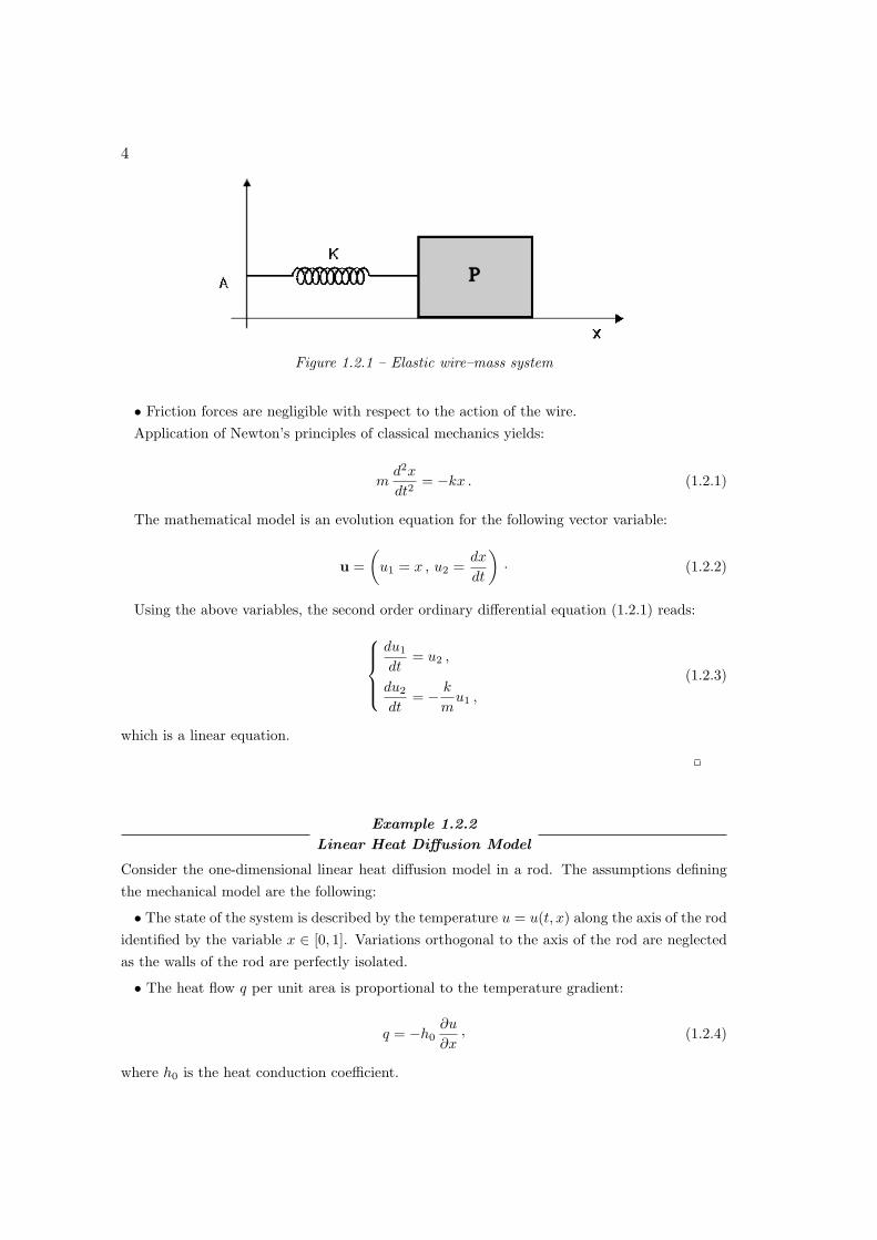
Consider, with reference to Figure 1.2.1, a mechanical system constituted by a mass m con-strained to translate along an horizontal line, say the x-axis. The location of the mass is iden-tified by the coordinate of its center of mass P , which is attached to an elastic wire stretchedwith ends in A and P . The assumptions defining the mechanical model are the following:
• The system behaves as a point mass with localization identified by the variable x.
• The action of the wire is a force directed toward the point A with module: T = k x.
4
Figure 1.2.1 – Elastic wire–mass system
• Friction forces are negligible with respect to the action of the wire.Application of Newton’s principles of classical mechanics yields:
md2x
dt2= −kx . (1.2.1)
The mathematical model is an evolution equation for the following vector variable:
u =(
u1 = x , u2 =dx
dt
)· (1.2.2)
Using the above variables, the second order ordinary differential equation (1.2.1) reads:
du1
dt= u2 ,
du2
dt= − k
mu1 ,
(1.2.3)
which is a linear equation.
Example 1.2.2
Linear Heat Diffusion Model
Consider the one-dimensional linear heat diffusion model in a rod. The assumptions definingthe mechanical model are the following:
• The state of the system is described by the temperature u = u(t, x) along the axis of the rodidentified by the variable x ∈ [0, 1]. Variations orthogonal to the axis of the rod are neglectedas the walls of the rod are perfectly isolated.
• The heat flow q per unit area is proportional to the temperature gradient:
q = −h0∂u
∂x, (1.2.4)
where h0 is the heat conduction coefficient.
5
• The material properties of the conductor are identified by the heat conduction coefficienth0 and heat capacity c0.
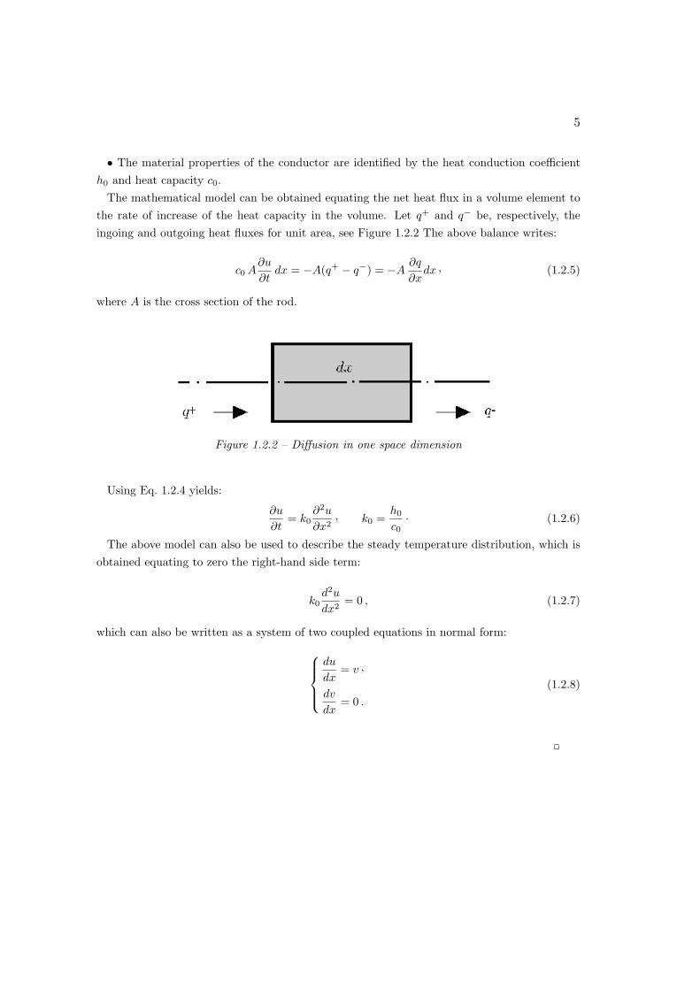
The mathematical model can be obtained equating the net heat flux in a volume element tothe rate of increase of the heat capacity in the volume. Let q+ and q− be, respectively, theingoing and outgoing heat fluxes for unit area, see Figure 1.2.2 The above balance writes:
c0 A∂u
∂tdx = −A(q+ − q−) = −A
∂q
∂xdx , (1.2.5)
where A is the cross section of the rod.
Figure 1.2.2 – Diffusion in one space dimension
Using Eq. 1.2.4 yields:
∂u
∂t= k0
∂2u
∂x2, k0 =
h0
c0· (1.2.6)
The above model can also be used to describe the steady temperature distribution, which isobtained equating to zero the right-hand side term:
k0d2u
dx2= 0 , (1.2.7)
which can also be written as a system of two coupled equations in normal form:
du
dx= v ,
dv
dx= 0 .
(1.2.8)

6
Example 1.2.3
Nonlinear Heat Diffusion Model
Nonlinearity may be related to the modelling of the heat flux phenomenon. For instance, ifthe heat flux coefficient depends on the temperature, say h = h(u), the same balance equationgenerates the following model:
∂u
∂t=
∂
∂x
[k(u)
∂u
∂x
], k(u) =
h(u)c0
. (1.2.9)
The reader with a basic knowledge of elementary theory of differential equations will be soonaware that the above two simple models generate interesting mathematical problems. In fact,Model 1.2.1 needs initial conditions for t = t0 both for u1 = u1(t) and u2 = u2(t), while Models1.2.2 and 1.2.3 need initial conditions at t = t0 and boundary conditions at x = 0 and x = 1for u = u(t, x).
The solution of the above mathematical problems ends up with simulations which visualizethe behavior of the real system according to the description of the mathematical model.
After the above examples, a definition of mathematical model can be introduced. Thisconcept needs some preliminary definitions referring to:
• Independent variables, generally time and space.
• State variables which are the dependent variables, that take values corresponding tothe independent variables.
Then the following concept can be introduced:
• Mathematical model, that is a set of equations which define the evolution of the statevariable over the dependent variables.
The general idea is to observe the phenomenology of a real system in order to extract itsmain features and to provide a model suitable to describe the evolution in time and space ofits relevant aspects. Bearing this in mind, the following definitions are proposed:
Independent variables
The evolution of the real system is referred to the independent variables which,
unless differently specified, are time t, defined in an interval (t ∈ [t0, T ]), which refers
the observation period; and space x, related to the volume V, (x ∈ V) which contains
the system.

7
State variable
The state variable is the finite dimensional vector variable
u = u(t,x) : [t0, T ]× V → IRn , (1.2.10)
where u = u1, . . . , ui, . . . , un is deemed as sufficient to describe the evolution of the
physical state of the real system in terms of the independent variables.
Mathematical model
A mathematical model of a real physical system is an evolution equation suitable
to define the evolution of the state variable u in charge to describe the physical state
of the system itself.
In order to handle properly a mathematical model, the number of equations and the dimensionof the state variable must be the same. In this case the model is defined consistent:
Consistency
The mathematical model is said to be consistent if the number of unknown depen-
dent variables is equal to the number of independent equations.
This means that one has to verify whether an equation belonging to the model can be obtainedcombining the remaining ones. If this is the case, that equation must be eliminated.
The space variable may be referred to a suitable system of orthogonal axes, 0(x, y, z) withunit vectors i, j, k, so that a point P is identified by its coordinates
P = P(x) = x i + y j + z k . (1.2.11)
The real physical system may be interacting with the outer environment or may be isolated.In the first case the interactions has to be modelled.
Closed and Open Systems
A real physical system is closed if it does not interact with the outer environment,
while it is open if it does.
The above definitions can be applied to real systems in all fields of applied sciences: engi-neering, natural sciences, economy, and so on. Actually, almost all systems have a continuousdistribution in space. Therefore, their discretization, that amounts to the fact that u is a finitedimensional vector, can be regarded as an approximation of physical reality.
In principle, one can always hope to develop a model which can reproduce exactly physicalreality. On the other hand, this idealistic program cannot be practically obtained consideringthat real systems are characterized by an enormous number of physical variables. This reasoningapplies to Example 1.2.1, where it is plain that translational dynamics in absence of frictionalforces is only a crude approximation of reality. The observation of the real behavior of the

8
system will definitively bring to identify a gap between the observed values of u1 and u2 andthose predicted by the model.
Uncertainty may be related also to the mathematical problem. Referring again to the aboveexample, it was shown that the statement of mathematical problems need u10 and u20, i.e. theinitial position and velocity of P , respectively. Their measurements are affected by errors sothat their knowledge may be uncertain.
In some cases this aspect can be dealt with by using in the model and/or in the mathematicalproblems randomness modelled by suitable stochastic variables. The solution of the problemwill also be represented by random variables, and methods of probability theory will have tobe used.
As we have seen, mathematical models are stated in terms of evolution equations. Exampleshave been given for ordinary and partial differential equations. The above equations cannot besolved without complementing them with suitable information on the behavior of the systemcorresponding to some values of the independent variables. In other words the solution refers tothe mathematical problem obtained linking the model to the above mentioned conditions. Oncea problem is stated suitable mathematical methods have to be developed to obtain solutionsand simulations, which are the prediction provided by the model.
The analysis of the above crucial problems, which is a fundamental step of applied mathe-matics, will be dealt with in the next chapters with reference to specific classes of equations.
1.3 Modelling Scales and Representation
As we have seen by the examples and definitions proposed in Section 1.2, the design ofa mathematical model consists in deriving an evolution equation for the dependent variable,which may be called state variable, which describes the physical state of the real system, thatis the object of the modelling process.
The selection of the state variable and the derivation of the evolution equation starts fromthe phenomenological and experimental observation of the real system. This means that thefirst stage of the whole modelling method is the selection of the observation scale. For instanceone may look at the system by distinguishing all its microscopic components, or averaginglocally the dynamics of all microscopic components, or even looking at the system as a wholeby averaging their dynamics in the whole space occupied by the system.
For instance, if the system is a gas of particles inside a container, one may either model thedynamics of each single particle, or consider some macroscopic quantities, such as mass density,momentum and energy, obtained averaging locally (in a small volume to be properly defined:possibly an infinitesimal volume) the behavior of the particles. Moreover, one may average thephysical variables related to the microscopic state of the particles and/or the local macroscopicvariables over the whole domain of the container thus obtaining gross quantities which representthe system as a whole.

9
Specifically, let us concentrate the attention to the energy and let us assume that energy maybe related to temperature. In the first case one has to study the dynamics of the particlesand then obtain the temperature by a suitable averaging locally or globally. On the otherhand, in the other two cases the averaging is developed before deriving a model, then themodel should provide the evolution of already averaged quantities. It is plain that the abovedifferent way of observing the system generates different models corresponding to differentchoices of the state variable. Discussing the validity of one approach with respect to the otheris definitively a difficult, however crucial, problem to deal with. The above approaches will becalled, respectively, microscopic modelling and macroscopic modelling.
As an alternative, one may consider the microscopic state of each microscopic componentand then model the evolution of the statistical distribution over each microscopic description.Then one deals with the kinetic type (mesoscopic) modelling which will be introduced inthis chapter and then properly dealt with later in Chapter 4. Modelling by methods of themathematical kinetic theory requires a detailed analysis of microscopic models for the dynamicsof the interacting components of the system, while macroscopic quantities are obtained, as weshall see, by suitable moments weighted by the above distribution function.
This section deals with a preliminary derivation of mathematical framework related to thescaling process which has been described above. This process will ends up with a classificationboth of state variables and mathematical equations. Simple examples will be given for eachclass of observation scales and models. The whole topic will be specialized in the followingchapters with the aim of a deeper understanding on the aforementioned structures.
Both observation and simulation of system of real world need the definition of suitable ob-servation and modelling scales. Different models and descriptions may correspond to differentscales. For instance, if the motion of a fluid in a duct is observed at a microscopic scale, eachparticle is singularly observed. Consequently the motion can be described within the frame-work of Newtonian mechanics, namely by ordinary differential equations which relate the forceapplied to each particle to its mass times acceleration. Applied forces are generated by theexternal field and by interactions with the other particles.
On the other hand, the same system can be observed and described at a larger scale consid-ering suitable averages of the mechanical quantities linked to a large number of particles, andthe model refers to macroscopic quantities such as mass density and velocity of the fluid. Asimilar definition can be given for the mass velocity, namely the ratio between the momentumof the particles in the reference volume and their mass. Both quantities can be measured bysuitable experimental devices operating at a scale of a greater order than the one of the singleparticle. This class of models is generally stated by partial differential equations.
Actually, the definition of small or large scale has a meaning which has to be related to thesize of the object and of the volume containing them. For instance, a planet observed as a rigidhomogeneous whole is a single object which is small with respect to the galaxy containing theplanet, but large with respect to the particles constituting its matter. So that the galaxy canbe regarded as a system of a large number of planets, or as a fluid where distances between

10
planets are neglected with respect to the size of the galaxy. Bearing all above in mind, thefollowing definitions are given:
Microscopic scale
A real system can be observed, measured, and modelled at the microscopic scale if
all single objects composing the system are individually considered, each as a whole.
Macroscopic scale
A real system can be observed, measured, and modelled at the macroscopic scale
if suitable averaged quantities related to the physical state of the objects composing
the system are considered.
Mesoscopic scale
A real system can be observed, measured, and modelled at the mesoscopic (kinetic)
scale if it is composed by a large number of interacting objects and the macroscopic
observable quantities related to the system can be recovered from moments weighted
by the distribution function of the state of the system.
As already mentioned, microscopic models are generally stated in terms of ordinary differ-ential equations, while macroscopic models are generally stated in terms of partial differentialequations. This is the case of the first two examples proposed in the section which follows.The contents will generally be developed, unless otherwise specified, within the framework ofdeterministic causality principles. This means that once a cause is given, the effect is deter-ministically identified, however, even in the case of deterministic behavior, the measurement ofquantities needed to assess the model or the mathematical problem may be affected by errorsand uncertainty.
The above reasoning and definitions can be referred to some simple examples of models, thisalso anticipating a few additional concepts which will be dealt in a relatively deeper way in thechapters which follow.
Example 1.3.1
Elastic Wire-Mass System with Friction
Following Example 1.2.1, let us consider a mechanical system constituted by a mass m con-strained to translate along a horizontal line, say the x-axis. The location of the mass is identifiedby the coordinate of its center of mass P , which is attached to an elastic wire stretched withends in A and P . The following assumption needs to be added to those of Model 1.2.1 definingthe mechanical model:
• Friction forces depend on the p-th power of the velocity and are direct in opposition withit.

11
Application of Newton’s model yields:
md2x
dt2= −kx− c
(dx
dt
)p
. (1.3.1)
The mathematical model, according to the definitions proposed in Section 1.2, is an evolutionequation for the variable u defined as follows:
u =(
u1 = x , u2 =dx
dt
)· (1.3.2)
Using the above variables, the second order ordinary differential equation (1.3.1) can bewritten as a system of two first order equations:
du1
dt= u2 ,
du2
dt= − k
mu1 − c
mup
2 ·(1.3.3)
The above example has shown a simple model that can be represented by an ordinary differ-ential equation, Eq. (1.3.3), which is nonlinear for values of p different from zero or one.
Observing Eq. (1.3.3), one may state that the model is consistent, namely there are twoindependent equations corresponding to the two components of the state variable. The physicalsystem is observed singularly, i.e. at a microscopic scale, while it can be observed that the modelis stated in terms of ordinary differential equations.
Linearity of the model is obtained if c = 0. On the other hand, if k is not a constant, butdepends on the elongation of the wire, say k = k0x
q a nonlinear model is obtained:
du1
dt= u2 ,
du2
dt= −k0
muq+1
1 ·(1.3.4)
Independently of linearity properties, which will be properly discussed in the next Chapter2, the system is isolated, namely it is a closed system. One should add, in the case of opensystems, to the second equation the action of the outer environment over the inner system. Asimple example is the following:
du1
dt= u2 ,
du2
dt= −k0
muq+1
1 +1m
F (t) ,(1.3.5)
where F = F (t) models the above mentioned action.

12
The above models, both linear and nonlinear, have been obtained linking a general back-ground model valid for large variety of mechanical systems, that is the fundamental principlesof Newtonian mechanics, to a phenomenological model suitable to describe, by simple analyticexpressions, the elastic behavior of the wire. Such models can be refined for each particularsystem by relatively more precise empirical data obtained by experiments.
The example which follows is developed at the macroscopic scale and it is related to the heatdiffusion model we have seen in Section 1.2. Here, we consider a mathematical model suitableto describe the diffusion of a pollutant of a fluid in one space dimension.
As we shall see, an evolution equation analogous to the one of Example 1.2.2 will be obtained.First the linear case is dealt with, then some generalizations, i.e. non linear models and diffusionin more than one space dimensions, are described.
Example 1.3.2
Linear Pollutant Diffusion Model
Consider a duct filled with a fluid at rest and a pollutant diffusing in the duct in the direction x
of the axis of the duct. The assumptions which define the mechanical model are the following:
• The physical quantity which defines the state of the system is the concentration of pollutant:
c = c(t, x) : [t0, T ]× [0, `] → IR+ , (1.3.6)
variations of c along coordinates orthogonal to the x-axis are negligible. The mass per unitvolume of the pollutant is indicated by ρ0 and is assumed to be constant.
• There is no dispersion or immersion of pollutant at the walls.
• The fluid is steady, while the velocity of diffusion of the pollutant is described by a phe-nomenological model which states that the diffusion velocity is directly proportional to thegradient of c and inversely proportional to c.
The evolution model, i.e. an evolution equation for c, can be obtained exploiting mass con-servation equation. In order to derive such equation let consider, with reference to Figure 1.2.2,the flux q = q(t, x) along the duct and let q+ and q− be the inlet and outlet fluxes, respectively.Under suitable regularity conditions, which are certainly consistent with the physical systemwe are dealing with, the relation between the above fluxes is given by:
q+ = q− +∂q
∂xdx . (1.3.7)
A balance equation can be written equating the net flux rate to the increase of mass in thevolume element Adx, where A is the section of the duct. The following equation is obtained:
ρ0 A∂c
∂tdx + A
∂(cv)∂x
dx = 0 , (1.3.8)

13
where v is the diffusion velocity which, according to the above assumptions, can be written asfollows:
v = −h0
c
∂c
∂x, (1.3.9)
and h0 is the diffusion coefficient.Substituting the above equation into (1.3.8) yields
∂c
∂t= k0
∂2c
∂x2, k0 =
h0
ρ0, (1.3.10)
which is a linear model.
Nonlinearity related to the above model may occur when the diffusion coefficient depends onthe concentration. This phenomenon generates the nonlinear model described in the followingexample.
Example 1.3.3
Nonlinear Pollutant Diffusion Model
Consider the same phenomenological model where, however, the diffusion velocity depends onthe concentration according to the following phenomenological model:
v = −h0h(c)
c
∂c
∂x, (1.3.11)
where h(c) describes the behavior of the diffusion coefficient with c. The model writes as follows:
∂u
∂t=
∂
∂x
(k(c)
∂c
∂x
), k(c) =
h(c)ρ0
. (1.3.12)
Phenomenological interpretations suggest:
k(0) = k(cM ) = 0 , (1.3.13)
where cM is the maximum admissible concentration. For instance:
k(c) = c(cM − c) , (1.3.14)
so that the model reads:
∂c
∂t= c(cM − c)
∂2c
∂x2+ (cM − 2c)
(∂c
∂x
)2
. (1.3.15)
14
The above diffusion model can be written in several space dimensions. For instance, technicalcalculations generate the following linear model:
Example 1.3.4
Linear Pollutant Diffusion in Space
Let us consider the linear diffusion model related to Example 1.3.2, and assume that diffusionis isotropic in all space dimensions, and that the diffusion coefficient does not depend on c. Inthis particular case, simple technical calculations yield:
∂c
∂t= k0
(∂2
∂x2+
∂2
∂y2+
∂2
∂z2
)c = k0 ∆c . (1.3.16)
The steady model is obtained equating to zero the right-hand side of (1.3.16):
(∂2
∂x2+
∂2
∂y2+
∂2
∂z2
)c = k0 ∆c = 0 . (1.3.17)
The above (simple) examples have given an idea of the microscopic and macroscopic mod-elling. A simple model based on the mesoscopic description will be now given and criticallyanalyzed. Specifically, we consider an example of modelling social behaviors such that the mi-croscopic state is defined by the social state of a certain population, while the model describesthe evolution of the probability density distribution over such a state. The above distributionis modified by binary interactions between individuals.
Example 1.3.5
Population Dynamics with Stochastic Interaction
Consider a population constituted by interacting individuals, such that:
• The microscopic state of each individual is described by a real variable u ∈ [0, 1], that isa variable describing its main physical properties and/or social behaviors. As examples, in thecase of a population of tumor cells this state may have the meaning of maturation or progressionstage, for a population of immune cells we may consider the state u as their level of activation.
• The statistical description of the system is described by the number density functions
N = N(t, u) , (1.3.18)
which is such that N(t, u) du denotes the number of cells per unit volume whose state is, attime t, in the interval [u, u + du].

15
If n0 is the number per unit volume of individuals at t = 0, the following normalization of N
with respect to n0 can be applied:
f = f(t, u) =1n0
N(t, u) . (1.3.19)
If f (which will be called distribution function) is given, it is possible to compute, undersuitable integrability properties, the size of the population still referred to n0:
n(t) =∫ 1
0
f(t, u) du . (1.3.20)
The evolution model refers to f(t, u) and is determined by the interactions between pairs ofindividuals, which modify the probability distribution over the state variable and/or the size ofthe population. The above ideas can be stated in the following framework:
• Interactions between pairs of individuals are homogeneous in space and instantaneous, i.e.without space structure and delay time. They may change the state of the individuals as wellas the population size by shifting individuals into another state or by destroying or creatingindividuals. Only binary encounters are significant for the evolution of the system.
• The rate of interactions between individuals of the population is modelled by the encounter
rate which may depend on the state of the interacting individuals
η = η(v, w) , (1.3.21)
which describes the rate of interaction between pairs of individuals. It is the number of encoun-ters per unit time of individuals with state v with individuals with state w.
• The interaction-transition probability density
A = A(v → u |v, w) , (1.3.22)
gives the probability density distribution of the transition, due to binary encounters, of theindividuals which have state v with the individuals having state w that, after the interaction,manufacture individuals with state u.
The product between η and A is the transition rate
T (v → u |v, w) = η(v, w)A(v → u |v, w) . (1.3.23)
• The evolution equations for the density f can be derived by balance equation which equatesthe time derivative of f to the difference between the gain and the loss terms. The gain termmodels the rate of increase of the distribution function due to individuals which fall into thestate u due to uncorrelated pair interactions. The loss term models the rate of loss in thedistribution function of u-individuals due to transition to another state or due to death.

16
Combining the above ideas yields the following model
∂f
∂t(t, u) =
∫ 1
0
∫ 1
0
η(v, w)A(v → u |v, w)f(t, v)f(t, w) dv dw
−f(t, u)∫ 1
0
η(u, v)f(t, v) dv . (1.3.24)
The above example, as simple as it may appear, gives a preliminary idea of the way a kinetictype modelling can be derived. This topic will be properly revisited in Chapter 4. At presentwe limit our analysis to observing that a crucial role is defined by the modelling of interactionsat the microscopic scale which allows the application of suitable balance equation to obtain theevolution of the probability distribution. At present, we can observe that since A(v → u |v, w)is a probability density, it satisfies
∫ 1
0
A(v → u |v, w) du = 1 , ∀ v, w ∈ [0, 1] . (1.3.25)
As a consequence, Eq. (1.3.24) implies
∫ 1
0
∂f
∂t(t, u) =
∂
∂t
∫ 1
0
f(t, u) = 0 , ∀ t ≥ 0 , (1.3.26)
and, due to the normalization,∫ 1
0
f(t, u) du = 1 . (1.3.27)
Therefore, the knowledge of f means knowing the time evolution of the moments
Ep(t) =∫ 1
0
up f(t, u) du , (1.3.28)
for p = 1, 2, . . .
1.4 Dimensional Analysis for Mathematical Models
Examples 1.2.1 and 1.3.2 can be properly rewritten using dimensionless variables. This pro-cedure should be generally, may be always, applied. In fact, it is always useful, and in somecases necessary, to write models with all independent and dependent variables written in adimensionless form by referring them to suitable reference variables. These should be properlychosen in a way that the new variables take value in the domains [0, 1] or [−1, 1].
The above reference variables can be selected by geometrical and/or physical argumentsrelated to the particular system which is modelled. Technically, let wv be a certain variable

17
(either independent or dependent), and suppose that the smallest and largest value of wv,respectively wm and wM , are identified by geometrical or physical measurements; then thedimensionless variable is obtained as follows:
w =wv − wm
wM − wm
, w ∈ [0, 1] . (1.4.1)
For instance, if wv represents the temperature in a solid material, then one can assumewm = 0, and wM = wc, where wc is the melting temperature for the solid.
In principle, the description of the model should define the evolution within the domain [0, 1].When this does not occur, then the model should be critically analyzed.
If wv corresponds to one of the independent space variables, say it corresponds to xv, yv, andzv for a system with finite dimension, then the said variable can be referred to the smallest andto the largest values of each variable, respectively, xm, ym, zm, and xM , yM , and zM .
In some cases, it may be useful referring all variables with respect to only one space variable,generally the largest one. For instance, suppose that xm = ym = zm = 0, and that yM = axM ,and zM = bxM , with a, b < 1, one has
x =xv
xM
, y =yv
xM
, z =zv
xM
, (1.4.2)
with x ∈ [0, 1], y ∈ [0, a], z ∈ [0, b].
Somehow more delicate is the choice of the reference time. Technically, if the initial time ist0 and tv is the real time, one may use the following:
t =tv − t0Tc − t0
, t ≥ 0 , (1.4.3)
where generally one may have t0 = 0. The choice of Tc has to be related to the actual analyticstructure of the model trying to bring to the same order the cause and the effect as both ofthem are identified in the model. For instance, looking at models in Example 1.2.1, the cause
is identified by the right-hand side term, while the effect is the left-hand term. The modelshould be referred to the observation time during which the system should be observed. Thistime should be compared with Tc.
Bearing all above in mind let us apply the above concepts to the statement in terms ofdimensionless variables of the two models described in Examples 1.2.1 and 1.3.2.
Example 1.4.1
Dimensionless Linear Elastic Wire-Mass System
Let us consider the model described in Example 1.2.1, with the addition of the following as-sumption:
• A constant force F is directed along the x-axis.

18
Therefore, the model can written as follows:
md2xv
dt2v= F − kxv . (1.4.4)
It is natural assuming ` = F/k, t = tv/Tc, and x = xv/`. Then the model writes:
m
kTc2
d2x
dt2= 1− x . (1.4.5)
Assuming:m
kTc2 = 1 ⇒ Tc
2 =m
k, (1.4.6)
yields
d2x
dt2= 1− x , (1.4.7)
which is a second order model.The evolution can be analyzed in terms of unit of Tc.
Example 1.4.2
Linear Dimensionless Pollutant Diffusion Model
Consider the model described in Example 1.3.2 which, in terms of real variables, can be writtenas follows:
∂cv
∂t= k0
d2cv
∂x2v
, k0 =h0
ρ0, (1.4.8)
It is natural assuming u = cv/cM , t = tv/Tc, and x = xv/`. Then, the model writes:
1Tc
∂u
∂t=
k0
`2∂2u
∂x2, (1.4.9)
Moreover, taking:
k0Tc
`2= 1 ⇒ Tc =
`2
k0
yields
∂u
∂t=
∂2u
∂x2. (1.4.10)
In particular Eq. (1.4.10) shows that the same model is obtained, after scaling, to describelinear diffusion phenomena in different media. Indeed, only Tc changes according to the material
19
properties of the media. This means that the evolution is qualitatively the same, but it evolvesin time with different speeds scaled with respect to Tc.
Writing a model in terms of dimensionless variables is useful for various reasons, both fromanalytical point of view and from the computational one, which will be examined in details inthe chapters which follow. One of the above motivations consists in the fact that the proceduremay introduce a small dimensionless parameter which characterizes specific features of theevolution equation, e.g. nonlinear terms, time scaling, etc. As we shall see in Chapter 2, theabove parameters allow the development of perturbation techniques such that the solution canbe sought by suitable power expansion of the small parameter.
1.5 Traffic Flow Modelling
Various models have been proposed in the preceding sections corresponding to the micro-scopic, macroscopic, and kinetic representation. This section will show how the same physicalsystem can be represented by different models according to the selection of different observationscales.
Let us consider the one dimensional flow of vehicles along a road with length `. First the inde-pendent and dependent variables which, in a suitable dimension form, can represent the relevantphenomena related to traffic flow are defined, then some specific models will be described.
In order to define dimensionless quantities, one has to identify characteristic time T andlength `, as well as maximum density nM and maximum mean velocity vM . Specifically:
nM is the maximum density of vehicles corresponding to bumper-to-bumper traffic jam;
vM is the maximum admissible mean velocity which may be reached by vehicles in the emptyroad.
It is spontaneous to assume vMT = `, that means that T is the time necessary to cover thewhole road length ` at the maximum mean velocity vM . After the above preliminaries, we cannow define dimensionless independent and dependent variables.
The dimensionless independent variables are:
• t = tr/T , the dimensionless time variable referred to the characteristic time T , where tr isthe real time;
• x = xr/`, the dimensionless space variable referred to the characteristic length of the road `,where xr is the real dimensional space.
The dimensionless dependent variables are:
• ρ = n/nM , the dimensionless density referred to the maximum density nM of vehicles;
• V = VR/vM , the dimensionless velocity referred to the maximum mean velocity vM , whereVR is the real velocity of the single vehicle;
• v = vR/vM , the dimensionless mean velocity referred to the maximum mean velocity vM ,where vR is the mean velocity of the vehicles;

20
• q, the dimensionless linear mean flux referred to the maximum admissible mean flux qM .
Of course a fast isolated vehicle can reach velocities larger that vM . In particular a limitvelocity can be defined
V` = (1 + µ)vM , µ > 0 , (1.5.1)
such that no vehicle can reach a velocity larger than V`. Both vM and µ may depend on thecharacteristics of the lane, say a country lane or a highway, as well as to the type of vehicles,say a slow car, a fast car, a lorry, etc.
The above variables can assume different characterization according to the modeling scaleswhich can be adopted for the observation and modeling. In particular, one may consider,according to the indications given in the previous sections, the following types of descriptions:
• Microscopic description: the state of each vehicle is defined by position and velocity asdependent variables of time.
• Kinetic (statistical) description: the state of the system is still identified by position andvelocity of the vehicles however their identification refers to a suitable probability distributionand not to each variable.
•Macroscopic description: the state is described by locally averaged quantities, i.e. density,mass velocity and energy, regarded as dependent variables of time and space
In detail, in the microscopic representation all vehicles are individually identified. Thestate of the whole system is defined by dimensionless position and velocity of the vehicles. Theycan be regarded, neglecting their dimensions, as single points
xi = xi(t) , Vi = Vi(t) , i = 1, . . . , N , (1.5.2)
where the subscript refers to the vehicle.
On the other hand, according to the kinetic (statistical) description, the state of thewhole system is defined by the statistical distribution of position and velocity of the vehicles.Specifically, it is considered the following distribution over the dimensionless microscopic state
f = f(t, x, V ) , (1.5.3)
where f dx dV is the number of vehicles which at the time t are in the phase domain [x, x +dx]× [V, V + dV ].
Finally, the macroscopic description refers to averaged quantities regarded as dependentvariables with respect to time and space. Mathematical models are stated in terms of evolutionequations for the above variables. If one deals with density and mean velocity, then models willbe obtained by conservation equations corresponding to mass and linear momentum:
ρ = ρ(t, x) ∈ [0, 1] , v = v(t, x) ∈ [0, 1] . (1.5.4)
21
Before describing a specific model for each of the above scales, it is necessary to show how theinformation recovered at the microscopic scale and by the kinetic representation can provide,by suitable averaging processes, gross quantities such as density and mass velocity.
In the microscopic presentation, one can average the physical quantities in (1.5.2) either atfixed time over a certain space domain or at fixed space over a certain time range. For instancethe number density u(t, x) is given by the number of vehicles N(t) which at the time t are in[x− h, x + h], say
u(t, x) ∼= N(t)2hnM
· (1.5.5)
A similar reasoning can be applied to the mean velocity
v(t, x) ∼= 1N(t)vM
N(t)∑
i=1
Vi(t) , (1.5.6)
where, of course, the choice of the space interval is a critical problem and fluctuations may begenerated by different choices.
In the kinetic representation, macroscopic observable quantities can be obtained, under suit-able integrability assumptions, as momenta of the distribution f , normalized with respect tothe maximum density nM so that all variables are given in a dimensionless form. Specifically,the dimensionless local density is given by
ρ(t, x) =∫ 1+µ
0
f(t, x, V ) dV , (1.5.7)
while the mean velocity can be computed as follows:
v(t, x) = E[V ](t, x) =q(t, x)u(t, x)
=1
ρ(t, x)
∫ 1+µ
0
V f(t, x, V ) dV . (1.5.8)
After the above preliminaries, we can now describe some specific models. Actually very simpleones will be reported in what follows, essentially with tutorials aims. The first model is basedon the assumption that the dynamics of each test vehicle is determined by the nearest field
vehicle.
Example 1.5.1
Follow the Leader Microscopic Model
The basic idea of this model, see Klar et al. (1996), is that the accelerationd2xi
dt2(t + T ) of the
i− th vehicle at time t + T depends on the following quantities:
• The speed Vi(t) of the vehicle at time t,
• The relative speed of the vehicle and of its leading vehicle at time t: Vi−1(t)− Vi(t),
• The distance between the vehicle and its leading vehicle at time t: xi−1(t)− xi(t).

22
Hence the ordinary differential equation which describes the model is as follows:
d2xi
dt2(t + T ) = a (Vi(t))m Vi−1(t)− Vi(t)
(xi−1(t)− xi(t))c, (1.5.9)
where T is the reaction time of the driver, and a,m, c, are parameters to be fitted to specificalsituations.
The model which will be described in what follows was proposed by Prigogine and Hermann(1971), and is based on the assumption that each driver, whatever its speed, has a programin terms of a desired velocity which can be computed by suitable experiments. Specificallyfd = fd(V ) denotes, in what follows, the desired-velocity distribution function, meaningthat fd(V )dx dV gives the number of vehicles that, at time t and position x ∈ [x, x+dx], desireto reach a velocity between V and V + dV .
Example 1.5.2
Prigogine Kinetic Model
Prigogine’s model describes the traffic flow according to the scheme:
∂f
∂t+ V
∂f
∂x= JP [f ] , (1.5.10)
where the operator JP is the sum of two terms:
JP [f ] = Jr[f ] + Ji[f ] , (1.5.11)
which describe the rate of change of f due to two different contributes:
• The relaxation term Jr, due to the behavior of the drivers of changing spontaneously speedto reach a desired velocity.
• The (slowing down) interaction term Ji, due to the mechanics of the interactions betweenvehicles with different velocities.
Moreover, it is assumed that the driver’s desire also consists in reaching this velocity withina certain relaxation time Tr, related to the normalized density and equal for each driver.
More in details, Prigogine’s relaxation term is defined by:
Jr[f ](t, x, V ) =1
Tr[f ](fd(V )− f(t, x, V )) , (1.5.12)
with
Tr[f ](t, x) = τu(t, x)
1− u(t, x), (1.5.13)

23
where τ is a constant. The relaxation time is smaller the smaller is the density; instead fordensity approaching to the bumper condition, u → 1, this term grows indefinitely.
The term Ji is due to the interaction between a test (trailing) vehicle and its (field) headingvehicle. It takes into account the changes of f(t, x, V ) caused by a braking of the test vehicle dueto an interaction with the heading vehicle: it contains a gain term, when the test vehicle hasvelocity W > V , and a loss term, when the heading vehicle has velocity W < V . Moreover, Ji isproportional to the probability P that a fast car passes a slower one; of course this probabilitydepends on the traffic conditions and so on the normalized density. Taking the above probabilitydefined by the local density yields:
Ji[f ](t, x, V ) = u(t, x)f(t, x, V )∫ 1+µ
0
(W − V )f(t, x, W ) dW . (1.5.14)
Hence the model finally writes:
∂f
∂t+ V
∂f
∂x=
1− u(t, x)τu(t, x)
(fd(V )− f(t, x, V )) + u(t, x)
× f(t, x, V )∫ 1+µ
0
(W − V )f(t, x, W ) dW . (1.5.15)
Example 1.5.3
Macroscopic Models
The macroscopic model which follows is based on conservation of mass and linear momentum,see Bellomo et al. (2002), which can be written as follows:
∂u
∂t+
∂
∂x(uv) = 0 ,
∂v
∂t+ v
∂v
∂x= g[u, v] ,
(1.5.16)
where g defines the average acceleration referred to each particle. Square brackets are usedto indicate that the model of g may be a functional of the arguments. In practice it maybe not simply a function of the variables, but also of their first order derivatives. The wordacceleration is used, when dealing with traffic flow models, to avoid the use of the term force
for a system where the mass cannot be properly defined.
It is worth stressing that the above framework simply refers to mass and momentum conser-vation, while energy is not taken into account. This choice is practically necessary for a systemwhere the individual behavior plays an important role on the overall behavior of the system.

24
As we have seen, models can be obtained by Eq. (1.5.16) with the addition of a phenomeno-logical relation describing the psycho-mechanic action g = g[u, v] on the vehicles. For instance,if one assumes (in dimensionless variables):
g[u, v] ≡ g[u] = − 1u
∂p
∂x, (1.5.17)
then, the following:
∂u
∂t+
∂
∂x(uv) = 0
∂v
∂t+ v
∂v
∂x= − 1
u
∂p
∂x,
(1.5.18)
is obtained, where p is the pressure. A possible relation is the equation of ideal gases: p = c uγ ,where c is a constant (in isothermal conditions).
If, instead of (1.5.17), we assume the following:
g[u, v] = − 1u
∂p
∂x+
23uRe
∂2v
∂x2, (1.5.19)
we have
∂u
∂t+
∂
∂x(uv) = 0 ,
∂v
∂t+ v
∂v
∂x= − 1
u
∂p
∂x+
23uRe
∂2v
∂x2.
(1.5.20)
Here Re = V0Lu0/µ with V0, L and u0 reference speed, length and density respectively, andµ > 0 a material parameter called viscosity. Re is a positive constant called Reynolds number,that gives a dimensionless measure of the (inverse of) viscosity. System (1.5.20) defines theequations of motion of a viscous, compressible fluid in one spatial dimension. As it is obvious,the presence or the absence of the viscous term leads to a change in the mathematical structureof the equations, with consequences in the properties of the model.
Let us stress again that the above models have to be regarded as simple examples proposedto show how different representation scales generate different models corresponding to the samephysical system.
1.6 Classification of Models and Problems
The above sections have shown that the observation and representation at the microscopicscale generates a class of models stated in terms of ordinary differential equations, while themacroscopic representation generates a class of models stated in terms of partial differentialequations. In details, the following definitions can be given:

25
Dynamic and static models
A mathematical model is dynamic if the state variable u depends on the time variable
t. Otherwise the mathematical model is static.
Finite and continuous models
A mathematical model is finite if the state variable does not depend on the space
variables. Otherwise the mathematical model is continuous.
A conceivable classification can be related to the above definitions and to the structure of thestate variable, as it is shown in the following table:
finite static u = ue Algebric
finite dynamic u = u(t) ODE
continuous static u = u(x) PDE
continuous dynamic u = u(t,x) PDE
Figure 1.6.1 — Classification of mathematical models
The above classification corresponds to well defined classes of equations. Specifically:
• finite dynamic models correspond to ordinary differential equations, ODEs;
• continuous dynamic models correspond to partial differential equations, PDEs.
Static models, both finite and continuous, have to be regarded as particular cases of thecorresponding dynamic models obtained equating to zero the time derivative. Therefore:
• finite static models correspond to algebraic equations;
• continuous static models correspond to partial differential equations with partialderivatives with respect to the space variables only.
As specific examples of static models, the following two examples correspond, respectively, toExample 1.2.1 and Example 1.3.5.
Example 1.6.1
Static Configurations of an Elastic Wire-Mass System
Consider, with reference to Figure 1.2.1, the mechanical system described in Example 1.2.1.Equating to zero the left hand side term, i.e. the time derivatives, yields, in the linear case, thefollowing model:
u2 = 0 ,
− k
mu1 = 0 ·
(1.6.1)

26
Similarly the nonlinear model writes:
u2 = 0 ,
− k1
mu1 − c
mup
2 = 0 .(1.6.2)
Example 1.6.2
Static Configurations of a Population Dynamics Model
The static configuration of the stochastic population dynamics model described in Example1.3.5 are obtained equating to zero the left side term of Eq. (1.3.24)
∫ 1
0
∫ 1
0
η(v, w)A(v → u |v, w)f(t, v)f(t, w) dv dw = f(t, u)∫ 1
0
η(u, v)f(t, v) dv . (1.6.3)
1.7 Critical Analysis Focusing on Complexity Topics
This chapter has been proposed as an introduction to modelling, classification and organi-zation of mathematical models and equations. It has been stated that a deeper insight intomathematical aspects can be effectively developed only if a well defined class of models (andequations) is effectively specialized. Therefore, the above relatively deeper analysis is postponedto the chapters which follow.
This section simply anticipates some topics and concepts which will be analyzed properly inthe chapters which follow. Specifically, we anticipate some ideas concerning model validation
and complexity problems in modelling.Referring to model validation one can state, in general, that a model can be regarded valid
if it is able to provide information on the evolution of a real system sufficiently near to thoseobtained by experiments on the real system. So far a conceivable modelling procedure needsthe development of the following steps:
• The real system is modelled by suitable evolution equations able to describe the evolution ofthe dependent variables with respect to the independent ones.
• Mathematical problems are generated by linking to the model all conditions necessary forits solution. These conditions should be generated by experimental measurements on the realsystem.
27
• The above problems can be possibly solved and the output of the simulations is comparedwith the experimental observations.
• If the distance (according to a concept to be properly defined in mathematical terms) betweenthe above simulations and experiments is less than a critical value fixed a priori, then the modelcan be regarded valid, otherwise revisions and improvements are necessary.
Unfortunately, the concept of validity is not universal, but it refers to the circumstancesrelated to the above comparisons. Indeed, a model which is valid to describe certain phenomena,may loose validity with reference to different phenomena. Therefore development of modelsand their application needs a constant critical analysis which can go on following a systematicanalysis and improvements of each model.
Referring now to complexity problems in modelling, it is worth stating that this conceptcan be applied to the real system, as well as to the model and to the mathematical problems. Inprinciple all systems of the real world are complex, considering that the number of real variablessuitable to describe each system may be extremely large, if not infinite. Once applied mathe-maticians try to constrain the real system into a mathematical model, i.e. into a mathematicalequation, then a selection of the variables suitable to describe the state of the real system isdone.
In other words, every model reduces the complexity of the real system through a simplifieddescription by a finite number of variables. Enlarging the number of variables makes themodel virtually closer to the real system. On the other hand this enlargement may causecomplexity in modelling. In fact a large number of variables may need experiments to identifythe phenomenological models related to the material behavior of the system, which may requirehigh costs to be realized, and, in some cases, may be impossible.
However, suppose that the applied mathematician is able to design a model by a large numberof variables, then the related mathematical problem may become too difficult to be dealt with.Technically, it may happen that the computational time to obtain a careful solution increasesexponentially with the number of variables. In some cases, mathematics may not even be able tosolve the above problems. The above concepts refer to complexity related to mathematical
problems. Once more, this is a critical aspects of modelling which involves a continuousintellectual effort of applied mathematicians.
It is plain that the attempt to reduce complexity may fall in contrast with the needs posedby validation. Let us anticipate some concepts related to validation of models. Essentially,a validation process consists in the comparison between the prediction delivered by the modeland some experimental data available upon observation and measurement of the real system.If this distance is “small”, then one may say that the model is valid. Otherwise it is not.
The above distance can be computed by a suitable norm of the difference between the variablewhich defines the state of the model and the measurement obtained on the real system relatedto the same variable. Of course, different norms have to be used according to the differentclasses of models in connection to the different representation scales.

28
Let us critically focus on some aspects of the validation problems and their interplay withcomplexity problems:
• The validation of a model is related to a certain experiment. Hence a validity statement holdsonly in the case of the phenomena related to the experiment. In different physical conditions,the model may become not valid.
• The evaluation of the distance between theoretical prediction and measurements needs theselection of a certain norm which needs to be consistent not only with the analytic structure ofthe model, but also with the data available by the measurements.
• The concept of small and large related to the evaluation of the deviations of the theoreticalprediction from the experimental data has to be related both to the size (in a suitable norm)of the data, and to the type of approximation needed by the application of the model to theanalysis of real phenomena.
• Improving the accuracy (validity) of a model may be contrasted by the complexity problemsconcerning both modelling and simulations. In some cases accuracy may be completely lost dueto errors related to complex computational problems
Mathematical modelling constantly supports the development of applied sciences with theessential contribution of mathematical methods. In the past centuries, a systematic use of mod-elling methods have generated classical equations of mathematical physics, namely equationsdescribing hydrodynamics, elasticity, electromagnetic phenomena etc. Nowadays, modellingrefers to complex systems and phenomena to contribute to the development of technologicalsciences.
Mathematical models already contribute, and in perspective will be used more and more,to the development of sciences directly related to quality of life, say, among others, biology,medicine, earth sciences.
Modelling processes are developed through well defined methods so that it is correct to talkabout the science of mathematical modelling. The first stage of this complex process isthe observation of the physical system which has to be modelled. Observation also means orga-nization of experiments suitable to provide quantitative information on the real system. Thena mathematical model is generated by proper methods to deal with mathematical methods.
Generally a mathematical model is an evolution equation which can potentially describe theevolution of some selected aspects of the real system. The description is obtained solvingmathematical problems generated by the application of the model to the description of realphysical behaviors. After simulations it is necessary to go back to experiments to validate themodel. As we shall see, problems are obtained linking the evolution equation to the so-calledinitial and/or boundary conditions. Indeed, the simplest differential model cannot predictthe future if its behavior in the past and on the boundaries of the system are not defined.
The above procedure will be revisited all along these Lecture Notes and it will be particu-larized with reference to specific models or class of models. However, simply with the aim ofintroducing the reader to some aspects of the statement of problems and development of math-

29
ematical methods, the previously described Examples 1.3.1 and 1.2.2 will be revisited withspecial attention to statement of problems and simulations.
Example 1.7.1
Simulations for the Elastic Wire-Mass Model
Consider the model proposed in Example 1.3.1 as it is described, in the nonlinear case, byEq. (1.3.3). Simulations should provide the evolution in time of the variables u1 = u1(t) andu2 = u2(t).
It is plain that the above evolution can be determined from the initial state of the system:
u10 = u1(t0) , u20 = u2(t0) . (1.7.1)
In other words, different behaviors correspond to different initial states. A very simple way(actually, as we shall discuss in Chapter 2, too simple) to obtain the above simulation consistsin developing a finite difference scheme organized as follows:i) Consider the discretization of the time variable:
It = t0, t1, . . . , ti, . . . , h = ti+1 − ti . (1.7.2)
ii) Given the initial state (1.7.1), compute, with reference to Eq. (1.3.3), the state u11 = u1(t1)and u21 = u2(t1) by the following scheme:
u11 = u10 + u20 h ,
u21 = u20 + h
(− k
mu10 − c
mup
20
).
(1.7.3)
iii) Continue the above scheme at the step (i + 1) of the discretization by the following scheme:
u1(i+1) = u1i + u2i h ,
u2(i+1) = u2i + h
(− k
mu1i − c
mup
2i
),
(1.7.4)
where u1i = u1(ti) and u2i = u2(ti).The mathematical problem is stated linking conditions (1.7.1) to the mathematical model,
while the related mathematical method is developed in items i) – iii).

30
Example 1.7.2
Simulations for Linear Heat Transfer Model
Consider the mathematical model proposed in Example 1.2.2 as it is described by Eq. (1.2.6).Similarly to Example 1.7.1, simulations should provide the evolution in time and space of thevariable u = u(t, x). Also in this case, the above simulations can be developed by appropriatemathematical methods, if additional information is given on the behavior of u at the initialtime and at the boundaries of the space domain.
Specifically, let us assume it is known the initial state of the system:
u0(x) = u(t0, x) , ∀x ∈ [0, 1] , (1.7.5)
and the behavior at the boundaries x = 0 and x = 1, say the fluxes:
α(t) = q(t, 0) , β(t) = q(t, 1) , ∀ t ≥ t0 . (1.7.6)
Different behaviors correspond to different initial and boundary states. A very simple (actu-ally too simple as we shall discuss in Chapter 3) way to obtain the above simulation consists indeveloping a finite difference scheme organized as follows:i) Consider the discretization (1.7.2) of the time variable, and the following discretization for
the space variable:
Ix = x0 = 0, x1, . . . , xj , . . . , xn = 1 , d = xj+1 − xj . (1.7.7)
ii) Compute, with reference to (1.2.4), the fluxes at the boundary of each tract (finite volume)[xj , xj+1] by their approximate values qj+1 = qj+1(t):
qj+1 = −h0
d(uj+1 − uj) , (1.7.8)
where uj = uj(t) = u(t, xj) , ∀ j = 1, · · ·n− 1iii) Apply the following scheme at each time and for each volume corresponding to the space
discretization:duj+1
dt∼= − 1
c0 d(qj+1 − qj) =
k0
d2(uj+1 − 2uj + uj−1) . (1.7.9)
iv) Apply the time discretization tod uj+1
d tas in Example 1.7.1.
The mathematical problem is stated linking conditions (1.7.5)–(1.7.6) to the mathematicalmodel, while the related mathematical method is developed in items i) – iv).
The reader should be aware that the above examples have been dealt with at an intuitiveand, may be, naive level and that the above topics have to be revisited in a deeper framework.

31
Then, at this stage, some simple remarks are proposed with the aim of pointing out some crucialfeatures of the modelling process, which will be specifically discussed in the various chapterswhich follow with direct reference to particular models.
• A mathematical model, although approximating the physical reality, should not hiderelevant features. In particular, it should not hide nonlinear behaviors or nonlinear features ofthe phenomena which is modelled.
• Analysis of mathematical models essentially means solution of mathematical problemsobtained by providing suitable initial and/or boundary conditions to the state equation. Thistype of analysis needs the development of mathematical methods that can be organized forclasses of models and which may differ for each class. Mathematical methods, according towhat we have said in the preceding item, should be those of nonlinear analysis. Linearityshould be regarded as a particular situation.
• Generally, mathematical problems are not as mathematicians wish. In other words, realsituations are not such that existence, uniqueness, and regularity of the solution can be proved.Often, mathematical problems are imposed by physical reality. In fact, it may often happen thatalthough some information on the solution is given, some features of the model (the parameters)or of the mathematical problem (initial or boundary conditions) cannot be measured. Inverseproblems are almost always ill posed. On the other hand, it is plain that the solution ofinverse-type problems is of relevant importance in the construction of mathematical models.
• Physical systems sometimes show stochastic behaviors. In some situations, even if themathematical model is of a deterministic type, the related mathematical problem may be ofa stochastic type. In fact, initial or boundary conditions cannot be measured precisely andthis type of information may be affected by some stochastic noise. Stochastic behaviors inmathematical models may be an unavoidable feature, and, consequently, suitable mathematicalmethods need to be developed in order to deal with stochastic problems.
• The modelling process may be regarded as a sort of loop that might be interrupted whenthere is a satisfactory agreement between simulation and observation of the phenomena.
• Modelling not only leads to a simulation of physical reality, but can also contribute toa deeper understanding of physical systems. Indeed, after the simulation, the experimentalobservation can be revisited and hopefully improved.
Part of the contents of a letter, Bellomo (1998), appeared on the review journal of theAmerican Society of Mechanical Engineers is reported as it summarizes some of the conceptswhich have been reported above.
It is worth pointing out that modelling is a creative science, which requires observation, initia-
tive, and invention. Modelling motivates applied mathematics which, on the other hand, needs
to support modelling and contributes to address the invention along mathematically reasonable
paths. Further mathematical models can often contribute to a deeper understanding of physical
reality. Indeed, the construction of a mathematical model contributes to discover the organized
32
structures of physical systems. Moreover, the simulation can point out behaviors which have
not been, or even cannot, be observed.
Then one may state that mathematical modelling constantly supports the development oftechnological and natural sciences by providing the essential contribution of the mathematicalmethods.
An additional complexity problem is related to scaling. It may happen, in the case of systemsconstituted by a large number of interacting elements that, although the dynamics of eachelement is well understood, the collective behavior of the whole system is not properly describedby the sum of the dynamics of each element. The complexity source is that collective behaviorsfollow a dynamics totally different from that of the behavior of a few entities. It is not simplya matter of selection of the proper scale, while models should take into account the fact thatin large systems, the various elements do not behave in the same way and individual behaviorscan play a relevant role in the overall evolution of the whole system.
This observation introduces the concept of complexity of living systems, and hence thechallenging problem of modeling living systems. This topic is dealt with in Chapter 4, howeversome preliminary observations can be anticipated for large systems of interacting individuals.
• Living systems have the ability to express specific strategies which depends on that of theother interacting individuals.
• This ability is heterogeneously distributed among individuals, while interactions are generallynot additive.
• Living systems operate out of equilibrium and have the ability to extract energy from thesurrounding environment for their own benefit.
Although the above remarks do not cover the whole variety of complexity features of livingsystems, a preliminary analysis can be referred to the example of models we have presented inthis chapter.
• All models of this chapter involve, with exception of Models 1.3.5 and 1.5.2, a description ofthe state of the system by deterministic variables.
• All models have been derived by a causality principle, namely by a relation between “cause”and “effect”. This relation is deterministic for most models besides, again, 1.3.5 and 1.5.2.
• Focusing on deterministic models, it can be observed that the causality principle is basedon rigorous relations either conservation or equilibrium equations. On the other hand, thederivation of the model needs phenomenological models concerning the material behavior ofthe system under consideration.
• The afore–said characteristics are generally related to experiments which are valid in steadyconditions, while the model is supposed to operate far from these special conditions.
This latter remark focus on one of the weakness of the modeling approach, which occurswhenever the closure of equilibrium and conservation equations is obtained by heuristic mate-rial models that are no supported by a robust theory. Due to this motivation, the definitionmathematical models is used. On the other hand, the use of models of mathematical

33
physics can be used when conservation and/or equilibrium equations are closed by a relationderived by a theory of mathematical physics.
Very different appears to be the panorama offered by models of living systems, where thecausality principle involves random variables. Moreover, the phenomenological model used toclose the equilibrium and/or conservation equations may, in some cases, be stated in probability.In fact, the heterogeneous distribution of the ability to express a certain strategy requires theuse of random variables and stochastic models for the interactions.
This specific characteristics and the modeling difficulty suggest to design explorative modelsrather than predictive ones. More precisely:
- Predictive models are supposed to depict the evolution of systems once the parameters of themodel have been properly identified.
- Explorative models are supposed to depict the scenario of all conceivable evolutions corre-sponding to all admissible values of the parameters.
The latter class of models is very important in the case of living systems, where one may beinterested to understand the behavior of the system corresponding to different interaction rulesinvolving the entities composing the system itself.
However, the two examples that have been presented in this Section have to be considered verysimple examples that need to be criticized. For instance, by the fact that interactions are linearlyadditive, while living systems generally undergo non-linear interactions; as an example, focusingon the vehicle traffic model, the passing probability does not depend by binary interactions only,but by the distribution of the vehicles in the whole interaction domains.
Therefore, the challenging topic we are talking about has to be treated within a well definedmathematical approach, possibly a mathematical theory, different from that widely used in thischapter. Accordingly, the modeling approach to living systems will be widely treated in thelast chapter of this monograph.

34
35
Chapter 2
Microscopic Scale Models andOrdinary Differential Equations
2.1 Introduction
This chapter deals with modeling and related mathematical problems within the frameworkof the microscopic observation scale. Modeling at the microscopic scale means, according to theclassification of models and equations proposed in Chapter 1, deriving an evolution equationfor each element constituting the system where each element is treated as a whole. Generally,the model is stated in terms of a system of ordinary differential equations.
More precisely, if m is the dimension of the state variable which defines the state of eachelement and n the number of elements, then the dimension of the system is n×m. Equationsare generally linked by the mutual interactions of the elements belonging to the system and byexternal actions on the elements of the system.
Microscopic modeling can be developed when the number of elements is somehow small(in some sense to be properly specified). Otherwise, when their number becomes large, thecomputational complexity to handle a large system of equations may involve difficulties whichcannot be technically dealt with. Actually, technical difficulties do not refer to the derivation ofthe model, but to the computational treatment of a system of equations too large to be handled:specifically the computational time may grow exponentially with the number of equations. Inthis case a different way of modeling can be developed in order to reduce complexity.
This chapter deals with models and problems which do not yet generate the above typeof computational complexity. This delicate matter cannot be hidden, being aware thatreducing complexity is one of the challenging aspects of the science of mathematical modeling.However the real complexity problem is the modelling of nonlinear interactions rather than theapproach based on assumption of linear superposition already discussed in Chapter 1.
After the above preliminaries, the contents and organization of this chapter can be described.Specifically, after this introduction:
– Section 2.2 deals with modeling methods at the microscopic scale. As we shall see, although

36
it is not possible to assess a unique procedure to derive a model, still some general rules can beidentified. Some specific examples will show how models can be derived within the mathematicalframework of ordinary differential equations.
– Section 2.3 presents a classification of ordinary differential equations, and the mathematicalstatement of the problems, which is obtained by linking the evolution equation to the conditionsthat are necessary to its solution. If these conditions are given corresponding to the initial valueof the independent variable, say t = t0, one has an initial-value problem, also called Cauchyproblem. Otherwise, if these quantities are given at both ends of the range of the independentvariable, say t = t0 and t = t1, one has a boundary-value problem.
– Section 2.4 deals with the representation of solutions to mathematical problems described inSection 2.3. Then an introduction to discretization methods is proposed to obtain quantitativeresults, that are the simulations related to the solution of the above problems. This topic isrelated both to initial and boundary value problems. The contents have to be regarded as anintroduction to computational methods. The reader will be introduced to topics which need tobe properly revisited by means of the essential contribution of the pertinent literature.
– Section 2.5 is concerned with the qualitative analysis of dynamical systems; in particular withstability definitions followed by methods to study linear and nonlinear stability.
– Section 2.6 deals with regular and singular perturbation methods developed to analyze thequalitative and quantitative behavior of solutions to initial value problems for finite models.
– Section 2.7 provides a brief introduction to the problem of bifurcation, analyzing the de-pendence of the equilibrium points and of their stability properties on the parameters of themodel.
– Section 2.8 develops a critical analysis on the contents of this chapter focused, as already men-tioned, on modelling and computational problems, looking ahead to modelling and simulationof living systems.
2.2 On the Derivation of Mathematical Models
In general, it is not reasonable to assess only one method to derive models at the micro-scopic scale. However some common lines can be identified. Therefore a conceivable modelingprocedure will be here described and applied in the derivation of some specific models.
Let us consider the following sequential steps which may be followed for the derivation offinite mathematical models:
Step 1. Phenomenological observation of the physical system which needs to be modeled.
Step 2. Identification of the various elements composing the system and of the dependent(state) variables suitable to describe the state of each element, and hence of the whole system.
Step 3. Modeling the causes which generate the dynamics and identification of the cause-effect relationships, as well as of the conservation equations (when they exist) of quantitiesrelated to the state of the system.
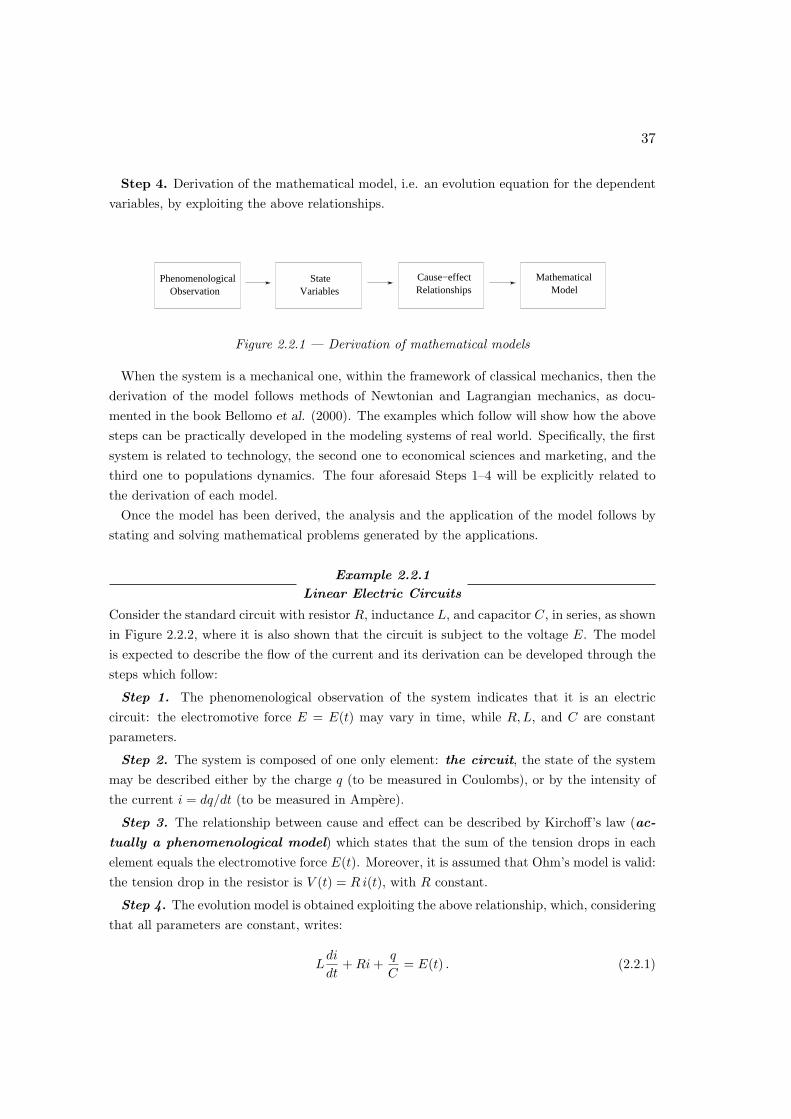
37
Step 4. Derivation of the mathematical model, i.e. an evolution equation for the dependentvariables, by exploiting the above relationships.
Observation VariablesStatePhenomenological Cause−effect
RelationshipsMathematical
Model
Figure 2.2.1 — Derivation of mathematical models
When the system is a mechanical one, within the framework of classical mechanics, then thederivation of the model follows methods of Newtonian and Lagrangian mechanics, as docu-mented in the book Bellomo et al. (2000). The examples which follow will show how the abovesteps can be practically developed in the modeling systems of real world. Specifically, the firstsystem is related to technology, the second one to economical sciences and marketing, and thethird one to populations dynamics. The four aforesaid Steps 1–4 will be explicitly related tothe derivation of each model.
Once the model has been derived, the analysis and the application of the model follows bystating and solving mathematical problems generated by the applications.
Example 2.2.1
Linear Electric Circuits
Consider the standard circuit with resistor R, inductance L, and capacitor C, in series, as shownin Figure 2.2.2, where it is also shown that the circuit is subject to the voltage E. The modelis expected to describe the flow of the current and its derivation can be developed through thesteps which follow:
Step 1. The phenomenological observation of the system indicates that it is an electriccircuit: the electromotive force E = E(t) may vary in time, while R, L, and C are constantparameters.
Step 2. The system is composed of one only element: the circuit, the state of the systemmay be described either by the charge q (to be measured in Coulombs), or by the intensity ofthe current i = dq/dt (to be measured in Ampere).
Step 3. The relationship between cause and effect can be described by Kirchoff’s law (ac-tually a phenomenological model) which states that the sum of the tension drops in eachelement equals the electromotive force E(t). Moreover, it is assumed that Ohm’s model is valid:the tension drop in the resistor is V (t) = R i(t), with R constant.
Step 4. The evolution model is obtained exploiting the above relationship, which, consideringthat all parameters are constant, writes:
Ldi
dt+ Ri +
q
C= E(t) . (2.2.1)

38
Considering that i is the derivative with respect to time of the charge q, the following secondorder model is derived:
d2q
dt2+
R
L
dq
dt+
q
LC=
E(t)L
, (2.2.2)
which can be written as a system of first order equations using the following variables:
u1 = q , u2 =dq
dt=
du1
dt,
so that the following system is obtained:
du1
dt= u2 ,
du2
dt= αu1 + βu2 + γE(t) ,
(2.2.3)
α = − 1LC
, β = −R
L, γ =
1L·
Remark 2.2.1. The derivation of the model (2.2.3), is obtained by particularizing the general
procedure described at the beginning of this section and visualized in Fig. 2.2.1.
Figure 2.2.2 — Electric Circuit.

39
Example 2.2.2
Modeling Marketing Dynamics
Consider the interaction within an economical system constituted by potential buyers withthe users of brand names in a closed marketing environment. Modeling the above systemshould provide the evolution in time of the numbers of the above interacting subjects. Themathematical model can be derived through the following steps:
Step 1. The system is constituted by potential buyers with the users of brand names in aclosed marketing environment. Interactions modify their number.
Step 2. The state of system is supposed to be described by the number u1 of potentialbuyers and the number u2 of users of brand names.
Step 3. The relationship between cause and effect can be described by a simple phenomeno-logical model such that u1 grows with time at a constant rate, namely the growth is linearlydepending on u2. On the other hand such a growth is contrasted by the interaction between u1
with up2, with p > 1, due to saturation phenomena. Similarly u2 grows due to the interaction
between u1 with uq2, with q > 1. On the other hand such a growth is contrasted by u2 due to
saturation of offer in the market.
Step 4. The model is obtained exploiting the above modeling of the cause and equating thecause to the effect, that is the time derivative of u1 and u2. The results is as follows:
du1
dt= α− βu1u
p2 + γu2 ,
du2
dt= βu1u
q2 − δu2 ,
(2.2.4)
where α defines the natural rate of growth of buyers, β refers to the decrease of buyers due totheir contact with brand names, while brand names increase the rate of growth of buyers asruled by the parameter γ. The parameter β is again used for their increase due to the contactwith buyers, while δ refers to decay of brand names.
Example 2.2.3
Population Dynamics
Consider a system of n interacting populations fully isolated with respect to the outer envi-ronment. Modeling the above system means obtaining the evolution in time of the numberof individuals of the above interacting populations. The mathematical model can be derivedthrough the following steps:
Step 1. The system is fully isolated, i.e., it is assumed that there is not interaction with theouter environment. Moreover, one assumes that the state of the system is simply described bythe number ui of individuals of each ith population.

40
Step 2. The cause–effect relationship is assessed by two phenomenological aspects. The firstaspect states that the population growth of the ith species linearly depends upon the numberof the individuals belonging to the said species. A second aspect states that the interactionbetween individuals of different species produces a decrease proportional to the product ofindividuals of the interacting species.
Step 3. The mathematical model is simply obtained equating the cause:
aiui − ui
n∑
j=1
bijuj , (2.2.5)
to the effect:
dui
dt= aiui − ui
n∑
j=1
bijuj · (2.2.6)
The above three simple models in Examples 2.2.1–2.2.3 show some technical differences. Thefirst model refers to one element only, the second one to a system of two elements, while thenumber of elements in the third one may be arbitrarily large. All models need to be rewrittenin terms of dimensionless variables after a proper selection of reference quantities as indicatedin Chapter 1. The derivation of the first model is based on principles of physics, more preciselymodels of material behaviour of circuits subject to electrical potential. The second and thirdmodel are simply related to a phenomenological interpretation of real systems. Surely thederivation is based on naive ideas that can be critically analyzed in the last section of thischapter.
More precisely, one may observe that the first Example 2.2.1 describes the interactions be-tween two objects, while the model 2.2.3 is concerned with the interactions among n popula-tions. Actually, the model is meaningful if n is small. Indeed, when the number of populationsbecomes large, interactions between pair of individuals may be affected by the presence of athird population. In other words, the coefficients are no longer constant, but may depend onthe state of the system. This is definitely an origin of complexity to be properly analyzed
2.3 Classification of Models and Mathematical Problems
Section 2.2 has shown that mathematical models can be derived at the microscopic scale inorder to describe the time evolution of a finite dimensional state variable: u = u(t), whereu is the set of dependent variables u = (u1, . . . , ui, . . . , un) defined over the domain [t0, t1] ofthe independent variable t.
This section deals with the classification of microscopic models which are structured in termsof ordinary differential equations, which will be assumed to be always written in dimensionless

41
form. The classification refers to models where the independent variable is the time t. However,it holds for any type of independent variable and it is based on the structure of the mathematicalequations.
Specifically, let us consider first systems of equations written in the commonly called normal
form :
du1
dt= f1(t, u1, . . . , un) ,
...
dun
dt= fn(t, u1, . . . , un) ,
(2.3.1)
which can be written, with obvious meaning of notation, in the compact vector form:
dudt
= f(t,u) . (2.3.2)
Another interesting class of models is the one which refers to higher-order scalar equations:
dnu
dtn= f
(t, u,
du
dt, · · · , dn−1u
dtn−1
)· (2.3.3)
The above equation can be rewritten in terms of a normal system of n equations in n unknownsby the change of variables:
u1 = u , u2 =du
dt, . . . , un =
dn−1u
dtn−1, (2.3.4)
which yields the normal form:
du1
dt= u2 ,
du2
dt= u3 ,
...
dun
dt= f(t, u1, . . . , un) .
(2.3.5)
This means, referring specifically to the class of equations represented in Eq. (2.3.1), that thefollowing classification can be given.

42
Linear Models
A system of ordinary differential equations (the model) is considered linear if it can
be written as follows:
du1
dt= a11(t)u1 + · · ·+ a1n(t)un + b1(t) ,
...
dun
dt= an1(t)u1 + · · ·+ ann(t)un + bn(t) ,
(2.3.6)
or in a compact form:
dudt
= A(t)u + b(t) , (2.3.7)
where A(t) is the n× n matrix of the coefficients aij(t), and b(t) is a column vector
with n components.
Linear Homogeneous Models
A linear system of ordinary differential equations (the model) is considered homo-
geneous if b(t) = 0 or in a compact form:
dudt
= A(t)u . (2.3.8)
Linear Models with Constant Coefficients
A system of ordinary differential equations (the model) is considered linear with
constant coefficients if the coefficients aij are constants. It can be written as
follows:
dudt
= Au + b(t) . (2.3.9)
A special case is when b is constant. Then, is A is nonsingular, the following change
of variable w = u + A−1b eliminates the nonhomogeneous term.
Nonlinear Models
A system of ordinary differential equations (the model) is considered nonlinear if
the terms fi are nonlinear functions of the dependent variables u.

43
Nonlinearly Weakly Perturbed Models
A system of ordinary differential equations (the model) is considered weakly per-
turbed semilinear if it can be written in the form:
dudt
= A(t)u + b(t) + ε f(t,u) , (2.3.10)
where ε is a small, dimensionless parameter.
A further aspect which plays an important role in modeling is the presence of time.
Autonomous Models
A system of ordinary differential equations (the model) is considered autonomous
if the time t does not explicitly appear as an argument of f . Otherwise, the model is
called nonautonomous.
For instance, in Eq. (2.3.9) A and b are, respectively, a constant matrix and a constantvector, so the system is autonomous. On the other hand, mathematical models presenting timedependent forcing terms are nonautonomous.
Remark 2.3.2. Linear homogeneous systems can be written in the following form:
dudt
= L(u) , (2.3.11)
where L(u) is a linear operator, i.e.
L(u1 + u2) = L(u1) + L(u2) , L(λu) = λL(u) , (2.3.12)
where λ is a real constant. On the other hand, nonlinear systems can be written as follow:
dudt
= N (u) , (2.3.13)
where N does not satisfy condition (2.3.12).
In some very general cases models may have even a structure of the type of the type:
f
(t, u,
du
dt, · · · , dnu
dtn
)= 0 · (2.3.14)
In this case, writing the model in normal form as indicated in Eq. (2.3.1) may be hard oreven impossible. Actually, the above very particular cases are not dealt with in these LectureNotes.
Let us now consider mathematical problems which are generated by the analysis of realsystems. These problems are stated by joining the evolution equation with the conditionsnecessary for its solution. Conditions for the solutions of problems are called initial and limit
conditions which may be defined as follows:
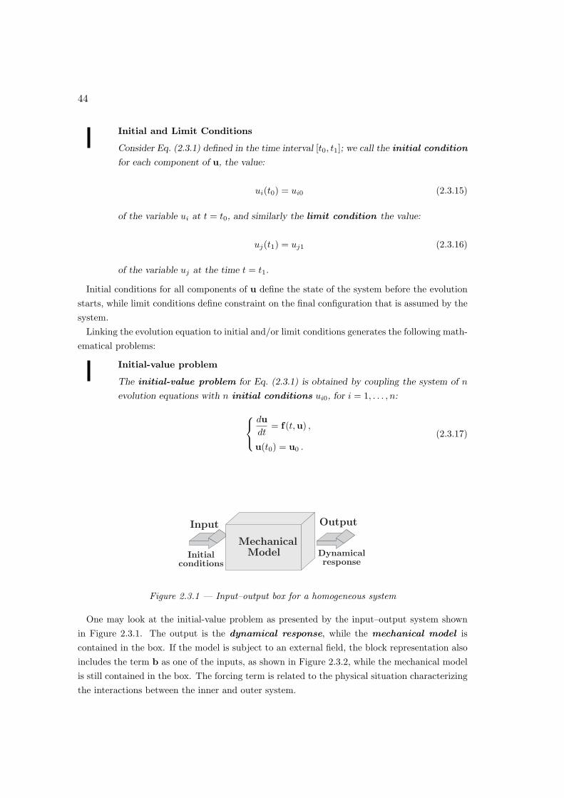
44
Initial and Limit Conditions
Consider Eq. (2.3.1) defined in the time interval [t0, t1]; we call the initial condition
for each component of u, the value:
ui(t0) = ui0 (2.3.15)
of the variable ui at t = t0, and similarly the limit condition the value:
uj(t1) = uj1 (2.3.16)
of the variable uj at the time t = t1.
Initial conditions for all components of u define the state of the system before the evolutionstarts, while limit conditions define constraint on the final configuration that is assumed by thesystem.
Linking the evolution equation to initial and/or limit conditions generates the following math-ematical problems:
Initial-value problem
The initial-value problem for Eq. (2.3.1) is obtained by coupling the system of n
evolution equations with n initial conditions ui0, for i = 1, . . . , n:
dudt
= f(t,u) ,
u(t0) = u0 .
(2.3.17)
Figure 2.3.1 — Input–output box for a homogeneous system
One may look at the initial-value problem as presented by the input–output system shownin Figure 2.3.1. The output is the dynamical response, while the mechanical model iscontained in the box. If the model is subject to an external field, the block representation alsoincludes the term b as one of the inputs, as shown in Figure 2.3.2, while the mechanical modelis still contained in the box. The forcing term is related to the physical situation characterizingthe interactions between the inner and outer system.
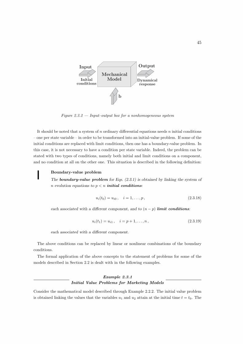
45
Figure 2.3.2 — Input–output box for a nonhomogeneous system
It should be noted that a system of n ordinary differential equations needs n initial conditions– one per state variable – in order to be transformed into an initial-value problem. If some of theinitial conditions are replaced with limit conditions, then one has a boundary-value problem. Inthis case, it is not necessary to have a condition per state variable. Indeed, the problem can bestated with two types of conditions, namely both initial and limit conditions on a component,and no condition at all on the other one. This situation is described in the following definition:
Boundary-value problem
The boundary-value problem for Eqs. (2.3.1) is obtained by linking the system of
n evolution equations to p < n initial conditions:
ui(t0) = ui0 , i = 1, . . . , p , (2.3.18)
each associated with a different component, and to (n− p) limit conditions:
ui(t1) = ui1 , i = p + 1, . . . , n , (2.3.19)
each associated with a different component.
The above conditions can be replaced by linear or nonlinear combinations of the boundaryconditions.
The formal application of the above concepts to the statement of problems for some of themodels described in Section 2.2 is dealt with in the following examples.
Example 2.3.1
Initial Value Problems for Marketing Models
Consider the mathematical model described through Example 2.2.2. The initial value problemis obtained linking the values that the variables u1 and u2 attain at the initial time t = t0. The
46
problems is as follows:
du1
dt= α− βu1u
p2 + γu2 ,
du2
dt= βu1u
q2 − δu2 ,
u1(t0) = u10 ,
u2(t0) = u20 ,
(2.3.20)
where u10 and u20 are given constants.
Example 2.3.2
Boundary Value Problems for a Population Model
Consider the mathematical model described through Example 2.2.3 for a two population dy-namics. A boundary value problem is obtained for example linking the values that the variableu1 attain at the initial time t = t0 and the one that u2 attain at the final time t = t1. Theproblem is as follows:
du1
dt= a1u1 − u1(b11u1 + b12u2) ,
du2
dt= a2u2 − u2(b21u1 + b22u2) ,
u1(t0) = u10 ,
u2(t1) = u21 .
(2.3.21)
2.4 Solution Schemes and Time Discretization
Section 2.3 has shown in that once a model has been properly derived, its practical applicationto the analysis of the behavior of real system needs the statement of a mathematical problem andthe related technical solution. It follows that mathematical methods for ordinary differentialequations should be developed to obtain quantitative simulations.
The development of analytic methods does not generally give sufficiently operative tools todeal with mathematical problems. In fact, the presence of nonlinearity in the model often(or almost always) requires the development of computational schemes and possibly scientificsoftware for the application of solution algorithms.
Several books are available in the literature which deal with analytic and/or computationalmethods. For instance, and among others, one may consider the book Marasco and Romano
47
(2001), into which, after the definition of the proper analytic background concerning existenceof solutions, stability properties, bifurcation analysis, various computational schemes are devel-oped with the aid of the Software Mathematica c©. A similar line is followed in the previouslycited book Bellomo et al. (2000), which is mainly oriented on the analysis of models of classicalmechanics. The interested reader is addressed to the above literature to obtain a relativelymore complete background on analytic and computational methods.
This section provides a concise description of solution schemes by analytic and discretizationmethods. Completeness is not claimed, the aim being simply to show how it is possible toobtain quantitative results from simulation of a large variety of class of problems. In details,this section is organized through four subsections which deal with the following topics:
i) existence of solutions to initial value problems;
ii) analytic methods for linear initial value problems;
iii) discretization schemes for initial value problems;
iv) boundary value problems.
2.4.1 Existence of solutions for initial value problems
This subsection deals with qualitative analysis related to the solution of the initial-value prob-lems for ordinary differential equations. Referring to the above class of problems, the followingdefinitions can be given:
Well-posedness
A problem is well formulated if the evolution equation is associated with the correct
number of initial (or boundary) conditions for its solution, while a problem is well
posed if the solution exists, it is unique and depends continuously on the initial data.
The main purpose of a model related to a certain physical system is to predict, for a certaintime interval, the behavior of the system starting from the knowledge of the state at the initialtime t0. The predictions of the model are then obtained by solving the initial-value problem.To do that, there are some basic requirements that a problem should satisfy:
i) The solution should exist, at least for the period of time desired;
ii) The solution should be unique;
iii) The solution should depend continuously on the initial data and on the parameters of themodel, so that if a small error is made in describing the present state, one should expect theeffect of this error to be small in the future.
As already stated, if these requirements are satisfied, then the initial-value problem is saidto be well posed.
Consider a norm in IRn, which might be, for instance, the Euclidean norm:
‖u‖ =
(n∑
i=1
u2i
) 12
, (2.4.1)
48
and give the following definition:
Lipschitz condition
A vector function f(t,u) satisfies a Lipschitz condition in a region D of the (t,u)-space if there exists a constant L (called Lipschitz constant), such that, for any
(t,u) and (t,v) in D one has:
∥∥f(t,u)− f(t,v)∥∥ ≤ L ‖u− v‖ . (2.4.2)
where both terms on the left-hand side of (2.4.2) are referred to the same instant of
time.
The Lipschitz condition is a property related both to continuity and differentiability. Indeed,it can be proved that if f(t,u) is defined in a bounded, closed, and convex domain D, and ifthe partial derivatives of f with respect to ui exist with:
maxi,j=1,...,n
sup(t,u)∈D
∣∣∣∣∂fi
∂uj
∣∣∣∣ ≤ M , (2.4.3)
then f satisfies a Lipschitz condition in D with a Lipschitz constant equal to M . We recallthat a domain is convex if any segment joining two points of the domain lies entirely within thedomain.
Of course, if f(t,u) satisfies a Lipschitz condition in D, f is a continuous function of u in Dfor each fixed t. The opposite is not true: for instance:
f(u) = 3√
u2
is continuous, however it does not satisfies the Lipschitz condition in any region containing theorigin. On the other hand, if f(t,u) is differentiable to respect to u, for all times, then it satisfiesthe Lipschitz condition, but the opposite it is not true, as it is shown by |u| that satisfies theLipschitz condition with constant L = 1 though it is not differentiable in u = 0.
Functions like:
f(u) = uq with q > 1 , or f(u) = cosh u ,
do not satisfy the Lipschitz condition in IR. In fact, roughly speaking, their derivative growswithout bound as u goes to infinity. However, they satisfy the Lipschitz condition in any closedbounded interval with Lipschitz constant equal to the maximum of the absolute value of thederivative in the interval.
Let us now consider, after the above preliminary definitions, the qualitative analysis of theinitial-value problem with initial time denoted by t0. Existence and uniqueness of solutions isstated by the following two theorems:

49
Theorem 2.1 Existence
If f(t,u) is continuous in the rectangle:
R =(t,u) : ‖u− u0‖ ≤ K , |t− t0| ≤ T
, (2.4.4)
then there exists at least one solution to the initial-value problem (2.3.17) and it is of
class C1 for |t− t0| ≤ T , where:
T = min
T,K
M
and M = max
(t,u)∈R‖f(t,u)
∥∥ .
Theorem 2.2 Uniqueness
If, in addition to the continuity condition of Theorem 2.1, the function f satisfies a
Lipschitz condition in R, then the solution u(t) to the initial-value problem (2.3.17) is
unique, and:
‖u(t)− u0‖ ≤ MT . (2.4.5)
Notice that the Lipschitz condition is not needed to assure the existence of a solution of theinitial-value problem. Instead, it is essential in the uniqueness proof. Actually, Theorem 2.1can be slightly improved, mainly by specializing the proofs to particular cases. For instance,existence results can be obtained for f(t,u) with a limited number of finite discontinuities.
Consider now the problem of the continuous dependence on the initial data, and let u
and u be the two solutions of the two initial-value problem (2.3.17) with initial data u(t0) = u0
and u(t0) = u0, respectively.
Theorem 2.3 Continuous dependence on the initial data
If f is continuous and satisfies the Lipschitz condition, then the following inequality holds:
∥∥u(t)− u(t)∥∥ ≤ ∥∥u0 − u0
∥∥eL|t−t0| , (2.4.6)
where L is the Lipschitz constant.
Finally, referring to the analysis of the continuous dependence on f , consider for t ∈[t0, t0 + T ] the initial-value problems:
dudt
= f(t,u) ,
u(t0) = u0 ,
and
dudt
= f∗(t,u) ,
u(t0) = u∗0 ,
(2.4.7)
with f and f∗ defined and continuous in a common domain D.
50
Theorem 2.4 Continuous dependence on f
If one of f or f∗ satisfies a Lipschitz condition with constant L and if:
∥∥f(t,u)− f∗(t,u)∥∥ ≤ ε , ∀ (t,u) ∈ D , (2.4.8)
then
∥∥u(t)− u∗(t)∥∥ ≤ ∥∥u0 − u∗0
∥∥eL|t−t0| +ε
L
[eL|t−t0| − 1
], (2.4.9)
where u(t) and u∗(t) are the solutions of the two initial-value problems defined in (2.4.7).
Although the above analysis answers the questions posed at the beginning of this sectionand can be applied to most of the initial-value problems occurring in nature, an importantquestion still remains unanswered: how large is the domain of the solution? The existenceresults shown above assure existence and uniqueness of the solution which may, however, leadto useless estimates on the existence interval.
Of course, the domain might be larger than the estimate given by the theorems, possiblyextending to all t ≥ t0. Then one needs criteria to determine the largest possible domain ofexistence. This question gives rise to the class of what is known as the extension theorems.Namely, extensions of the solution can be developed if one can prove that the norm of thesolution does not grow too fast. This type of analysis is often based on a deep understandingof the qualitative properties of the system. For instance boundness properties can be recoveredby a qualitative analysis of energy conservation. Of course, one needs to prove that the a priori
estimates hold true in the same function space where the local existence theorem has beenstated. This type of analysis can be recovered in the classical literature on ordinary differentialequations, see for example Pontriaguine (1975).
2.4.2 Analytic methods for linear initial value problems
In general, analytic solutions can be sought for in the case of linear systems of ordinarydifferential equations. The qualitative analysis of linear systems is widely dealt with in theliterature and can be approached in several ways. Some general results can be summarizedhere:
Remark 2.4.1. Any linear system:
dudt
= A(t)u + b(t) , (2.4.10)
with continuous coefficients on a time interval [0, T ] satisfies the Lipschitz condition with
L =n∑
i,j=1
maxt∈I
|Aij(t)| . (2.4.11)
51
Remark 2.4.2. The initial-value problem:
dudt
= A(t)u + b(t) ,
u(t0) = u0 ,
(2.4.12)
with Aij(t) and bi(t) defined and continuous for |t−t0| ≤ T , has a unique solution for |t−t0| ≤ T ,
by Theorems 2.1–2.2.
Remark 2.4.3. If u1(t), . . . ,um(t) are m solutions of the homogeneous linear system:
dudt
= A(t)u , u ∈ IRn , (2.4.13)
then any linear combination:
m∑
i=1
Ciui(t) , C1, . . . , Cm ∈ IR (2.4.14)
is still a solution of (2.4.13).
Theorem 2.5 Solutions of the Linear Homogeneous Models
There exist n linearly independent solutions u1, . . . ,un of (2.4.13) such that any solution
of (2.4.13) can be written as follows:
u(t) =n∑
i=1
Ciui(t) , (2.4.15)
for suitable C1, . . . , Cn ∈ IR.
Remark 2.4.4. The initial value problem:
dudt
= A(t)u ,
u(t0) = u0 ,
(2.4.16)
is solved by imposing the n initial conditions to u(t), given by (2.4.15), to find the values of the
constants C1, . . . , Cn.
A set of independent solutions for the homogeneous problem is called a fundamental set
and it can be ordered into a matrix:
U(t) =
u11(t) · · · u1n(t)...
. . ....
un1(t) · · · unn(t)
(2.4.17)

52
called the fundamental matrix.The above results can be exploited to obtain also analytic solutions of the nonhomogeneous
linear Eq. (2.4.10):
Theorem 2.6 Solutions of the Linear Models
Any solution of Eq.(2.4.10) can be written as follows:
u(t) =n∑
i=1
Ciui(t) + u(t) , (2.4.18)
for suitable coefficients C1, . . . , Cn ∈ IR, where u1(t), . . . ,un(t) is a fundamental set
for the homogeneous system (2.4.13) associated to (2.4.10), and u is a solution of
Eq. (2.4.10).
Summarizing the results stated in the above Theorems, the solution of a linear initial valueproblem (2.4.12) is obtained according to the following steps:
Step 1. Find a fundamental set u1(t), . . . ,un(t) for the homogeneous system (2.4.13) asso-
ciated to (2.4.10).
Step 2. Find a solution u of the nonhomogeneous system (2.4.10). This step sometimes can
be made by inspection, otherwise one can use the rule which determines u(t) as one of the
following functions:
u(t) = U(t)∫
U−1(t)b(t) dt , (2.4.19)
where U is the fundamental matrix defined by the functions obtained in Step 1, which amounts
to choosing a constant of integration.
Step 3. Impose the n initial conditions to (2.4.18) to find the values of the coefficients
C1, . . . , Cn.
In the case of systems of ordinary differential equations with constant coefficients:
dudt
= Au , u ∈ IRn , (2.4.20)
it is possible to give a general procedure to complete Step 1, and Step 2 can be developed in asimplified way. In fact, one can look for solutions in the form:
u(t) = veλt . (2.4.21)
Substituting (2.4.21) into (2.4.20) indicates that λ and v have to satisfy:
(A− λI)v = 0 . (2.4.22)

53
Hence, they have to be an eigenvalue and the corresponding eigenvector of the matrix A. De-tailed calculations differ technically according to the fact that the number of distinct eigenvaluesdiffers from n or is the same. In particular
• If A has n linearly independent eigenvectors v1, . . . ,vn corresponding to the eigenvaluesλ1, . . . , λn (which need not all be distinct and may be complex), then the solution of (2.4.20)is:
u = C1v1eλ1t + · · ·+ Cnvneλnt . (2.4.23)
A complex conjugate pair of eigenvalues λr ± iλi and eigenvectors vr ± ivi gives rise to asolution:
u = (Cr + iCi)(vr + ivi)e(λr+iλi)t + (Cr − iCi)(vr − ivi)e(λr−iλi)t
= 2eλrt[(
Crvr − Civi
)cos(λit)−
(Crvi + Civr
)sin(λit)
]. (2.4.24)
This matter has to be dealt with differently if there are eigenvalues with multiplicity r > 1and p < r corresponding eigenvectors. Without entering into details, we consider just thefollowing particular case:
• If A has n − 2 distinct eigenvalues λ1, . . . , λn−2 with corresponding distinct eigenvectorsv1, . . . ,vn−2 and a double eigenvalue λn−1 = λn = λ corresponding to a single eigenvector v,the solution of (2.4.20) is as follows:
u = C1v1eλ1t + · · ·+ Cn−2vn−2e
λn−2t +[Cn−1v + Cn(w + vt)
]eλt , (2.4.25)
where w is a solution of (A− λI)w = v.The case of a single equation of order n:
andnu
dtn+ · · ·+ a1
du
dt+ a0u = 0 (2.4.26)
is somewhat simpler since the procedure can be reduced to the solution of what is commonlycalled the characteristic equation:
anλn + · · ·+ a1λ + a0 = 0 . (2.4.27)
A real root λ corresponds to the solution (c0 + · · ·+ cµtµ)eλt , where µ is the multiplicity ofλ. A complex conjugate pair, λ+ = λr + iλi, and λ− = λr − iλi, corresponds to the solution:
eλrt[(c0 + . . . + cµtµ) cos λit + (d0 + . . . + dµtµ) sin λit
], (2.4.28)
where again µ is the multiplicity of λ+.
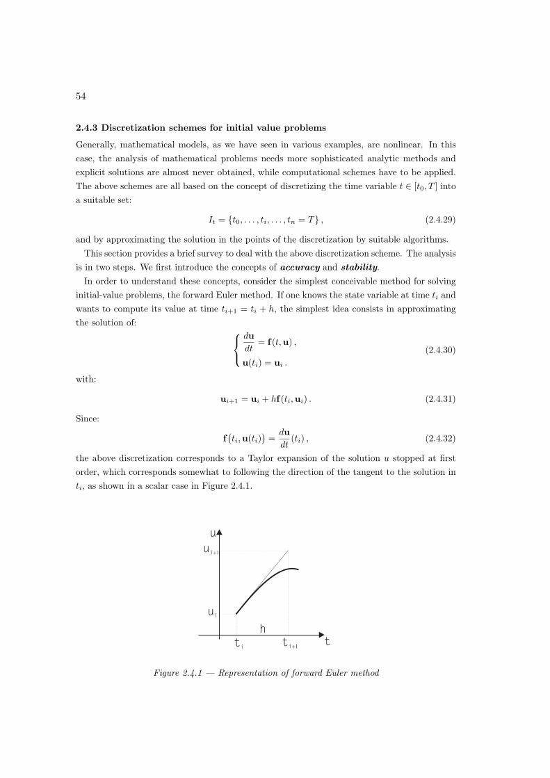
54
2.4.3 Discretization schemes for initial value problems
Generally, mathematical models, as we have seen in various examples, are nonlinear. In thiscase, the analysis of mathematical problems needs more sophisticated analytic methods andexplicit solutions are almost never obtained, while computational schemes have to be applied.The above schemes are all based on the concept of discretizing the time variable t ∈ [t0, T ] intoa suitable set:
It = t0, . . . , ti, . . . , tn = T , (2.4.29)
and by approximating the solution in the points of the discretization by suitable algorithms.This section provides a brief survey to deal with the above discretization scheme. The analysis
is in two steps. We first introduce the concepts of accuracy and stability.In order to understand these concepts, consider the simplest conceivable method for solving
initial-value problems, the forward Euler method. If one knows the state variable at time ti andwants to compute its value at time ti+1 = ti + h, the simplest idea consists in approximatingthe solution of:
dudt
= f(t,u) ,
u(ti) = ui .
(2.4.30)
with:
ui+1 = ui + hf(ti,ui) . (2.4.31)
Since:
f(ti,u(ti)
)=
dudt
(ti) , (2.4.32)
the above discretization corresponds to a Taylor expansion of the solution u stopped at firstorder, which corresponds somewhat to following the direction of the tangent to the solution inti, as shown in a scalar case in Figure 2.4.1.
u
t
h
ti+1t
i
ui+1
ui
Figure 2.4.1 — Representation of forward Euler method

55
Truncation Error
The truncation error Terr is defined as the norm of the difference between the
solution to the differential equation and the numerical solution divided by the time
step used in the numerical scheme.
In the case of forward Euler method it can be proved, under suitable regularity assumptions,that for each component:
Terr∼= − h
2d2u
dt2(ξ) , ξ ∈ (ti, ti+1) , (2.4.33)
where ξ changes from component to component.
Accuracy
If the truncation error goes like hp, the method is pth order, which means that
halving the step divides the error by 2p. This is what is generally meant by accuracy
of the method.
From (2.4.33), for the forward Euler method the error goes like h and one has a first ordermethod.
Another important requirement of a numerical scheme is that the time step has to be chosenso that the scheme is absolutely stable:
Absolute Stability
A numerical scheme is absolutely stable in a point ah of the complex plane if a
sequence ui generated by the method applied to the model:
du
dt= au , (2.4.34)
with time step ∆t = h is bounded for i → +∞.
Stability Region
The stability region is the set of points ah in the complex plane for which the
method is absolutely stable
It can be proved that each scheme is characterized by a stability region, which can be usedto determine a condition on the time step to be used in the integration. The procedure to beused is the following:
Step 1. Starting from a nonlinear model, consider its linearized form:
dudt
= Au , (2.4.35)
obtained for instance by linearization about the initial condition;

56
Step 2. Compute the eigenvalues λ1, . . . , λn of A, the so-called spectrum of the linearizedmodel;
Step 3. Choose, if possible, a not too restrictive time step h such that hλ1, . . ., hλn allbelong to the stability region.
Therefore, the numerical errors are not amplified as the integration is continued. If, instead,there are some eigenvalues which remain outside the stability region, then one must be awarethat the numerical errors grow exponentially in time. The literature on computational methodsreports about a large variety of algorithms to obtain simulations of finite models. The interestedreader is addressed to Chapter 3 of the book Bellomo and Preziosi (1995) as well as to Marascoand Romano (2001) for computational schemes.
Consider, as an example of algorithm, the Runge–Kutta methods which are very popularfor their adaptability and versatility and work quite well for all nonstiff problems. They areobtained by evaluating the function f at different values of t and u, and by suitably combiningof these values. In this way it is possible to obtain methods of any order of accuracy. Forinstance, one has:
2nd order : ui+1 = ui +h
2
(K1 + K2
), (2.4.36)
where
K1 = f(ti,ui) , K2 = f(ti + h,ui + hK1) . (2.4.37)
3rd order : ui+1 = ui +h
6
(K1 + 4K2 + K3
), (2.4.38)
where
K1 = f(ti,ui) ,
K2 = f(
ti +h
2,ui +
h
2K1
),
K3 = f(ti + h,ui + h(2K2 −K1)
).
(2.4.39)
4th order : ui+1 = ui +h
6
(K1 + 2K2 + 2K3 + K4
), (2.4.40)
where
K1 = f(ti,ui) ,
K2 = f(
ti +h
2,ui +
h
2K1
),
K3 = f(
ti +h
2,ui +
h
2K2
),
K4 = f(ti + h,ui + hK3) .
(2.4.41)

57
Recalling that the initial-value problem with initial condition u(ti) = ui can be written inintegral form as:
u(t) = ui +∫ t
ti
f(s,u(s)
)ds , (2.4.42)
and, in particular,
u(ti+1) = uti+
∫ ti+1
ti
f(s,u(s)
)ds , (2.4.43)
it can be observed that both the third-order and the fourth-order methods are closely relatedto Simpson’s rule applied to the integrals in (2.4.43).
The stability regions of the second-order method has an ellipsoidal shape, while that of thethird-order and fourth-order methods are bean-like shaped.
Third-order and fourth-order Runge–Kutta methods are recommended in dealing with prob-lems for which the spectrum is not available, since they include both a part of the imaginaryaxis and a part of the negative real axis. The disadvantage of these schemes is that severalevaluations of f have to be performed per time step and therefore if the computation of f
is very heavy, this method may demand an excessive amount of labor per step and becomesinconvenient.
Runge–Kutta methods have the property of being self-starting as well as adaptive. In otherwords, the time step can be changed at any moment according to an estimate of the localerror. Unfortunately, it is not trivial to get the above estimate of time step. In this case, tobe practical, the time step has then to be decreased if the difference between the two values(over h) is larger than a specified maximum tolerance and can be increased if this difference issmaller than the minimum required tolerance. Of course, this checking is time consuming.
2.4.4 On boundary value problems
Boundary-value problems for ordinary differential equations with time as independent variableoften arise in several applications. For example when some of the initial conditions at t = t0
cannot be measured and are replaced by the corresponding conditions at a certain control time,say t = t1, where their identification is possible.
Finding a solution to boundary-value problems is not an easy task. We remember that initial-value problems generally have unique solutions, while some boundary-value problems may havemore than one solution and others have no solutions at all, as it will be shown in the Example2.4.1 in what folows.
An existence theorem may be formulated for linear boundary-value problems. Here, we willrefer to a linear second order problem:
d2u
dt2+ a1(t)
du
dt+ a0(t)u = b(t) ,
u(t0) = u0 ,
u(t1) = u1 ,
(2.4.44)

58
and consider the following theorem:
Theorem 2.7 Existence and uniqueness
If a0, a1, and b are continuous in [t0, t1] and if
t1 − t0 <
2A1
if a0(t) = 0 ,
2
√A2
1 + 2A0 −A1
A0otherwise ,
(2.4.45)
where
|a0(t)| ≤ A0 and |a1(t)| ≤ A1 ∀t ∈ [t0, t1] ,
then the boundary-value problem (2.4.44) has a unique solution in [t0, t1].
Remark 2.4.5. When the existence of the solution of a linear boundary value problem is
assured (for example from Theorem 2.7), we can apply to the problem the results of Theorems
2.5–2.6. Then, imposing the initial and/or boundary conditions we get the solution of the
problem.
In order to clarify the importance of the existence and uniqueness issues related to boundary-value problems, consider the following example.
Example 2.4.1
Nonuniqueness and Buckling of a Rod
Consider a simple mass-spring system governed by the ordinary differential equation:
d2u
dt2+ Ω2u = 0 , (2.4.46)
where Ω2 = k/m, which has solution:
u(t) = C1 cos(Ω t) + C2 sin(Ω t) . (2.4.47)
If we join to (2.4.46) the initial conditions:
u(0) = u0 anddu
dt(0) = u′0 , (2.4.48)
the unique solution is:
u(t) = u0 cos(Ωt) +u′0Ω
sin(Ωt) . (2.4.49)
In a similar way, if we join to (2.4.46) the boundary conditions:
u(0) = u0 and u(T ) = uT , (2.4.50)

59
with T 6= hπ/Ω, h ∈ N, we again have a unique solution:
u(t) = u0 cos(Ωt) +uT − u0 cos(ΩT )
sin(ΩT )sin(Ωt) . (2.4.51)
If T = hπ/Ω, the boundary-value problem has no solution at all if uT 6= (−1)hu0, andinfinitely many solutions given by:
u(t) = u0 cos(Ωt) + C sin(Ωt) , ∀C ∈ IR , (2.4.52)
if uT = (−1)hu0.
The existence theorem considered above assures existence and uniqueness only if:
T <2√
2Ω
<π
Ω. (2.4.53)
Using the following argument this result can be used to explain the buckling of a rod. Considera rod of length T subject at its ends to a compressive load F , as shown in Figure 2.4.2. Thelinear theory of elasticity tells us that for small deformations the angle of deflection u of the rodcan be found by solving (2.4.46) with Ω2 = F/(EI), where E is Young’s modulus of elasticityfor the rod, and I is the moment of inertia of the cross section of the rod about its axis.
Figure 2.4.2 — Buckling of a rod: (a) small loads, (b) large loads
The previous discussion can then be reprocessed in the following terms: if T < π/Ω, that isif F < EIπ2/T 2, then there is no deflection, but as soon as F reaches the critical compressiveload (first buckling load) F = EIπ2/T 2, the solution is not unique and no longer small, whichalso indicates a failure of the linear theory of elasticity to model the situation.

60
2.5 Stability Methods
As already mentioned, it is possible to give a general procedure to obtain analytic solutionsonly for some classes of linear differential equations or for very special nonlinear problems. Onthe other hand, it is impossible in most cases to find analytic solutions. It is then desirable tohave at least some knowledge on the qualitative behavior of the solution.
In details, this Section is organized in three subsection which follows this brief introduction.The first subsection proposes some preliminary definitions, while the next two subsections ex-plain suitable methods for the analysis of the stability of equilibrium configurations, respectivelythe linear stability method the first subsection, and the nonlinear stability method the secondone.
2.5.1 Stability Definitions
In view of the study of the equilibrium configurations and their stability of a mathematicalmodel, we introduce the following definition:
Equilibrium points
Consider the autonomous system of ordinary differential equations:
dudt
= f(u) . (2.5.1)
The states ue such that:
f(ue) = 0 (2.5.2)
are called the equilibrium points. If u(t0) = ue, then u(t) = ue for all times.
It is trivial to verify that if an equilibrium point is occupied initially, it is maintained for alltimes.
The next problem is to decide whether an initially perturbed system gradually returns back tothe equilibrium point, or at least remains next to it, or wanders away. The following definitionsare given:
Stability and instability of equilibrium points
The equilibrium state ue is said to be stable if for any ε > 0 it is possible to find a
δ(ε) > 0 such that for any initial condition u(t0) with:
∥∥u(0)− ue
∥∥ < δ(ε) , (2.5.3)
one has that:∥∥u(t)− ue
∥∥ < ε ∀ t ≥ t0 . (2.5.4)
An equilibrium state that is not stable is called unstable.

61
Asymptotic stability and basin of attraction
A stable equilibrium point ue is also asymptotically stable if there is a neighborhood
De of ue such that for u(t0) ∈ De, one has:
limt→+∞
∥∥u(t)− ue
∥∥ = 0 . (2.5.5)
The largest possible De is called the basin of attraction of ue and is denoted in the
following by Be.
The definition of stability has a local meaning. Indeed, if we want that the system remains,within a given tolerance, near ue, the initial condition has to be sufficiently close to ue. Ingeneral an equilibrium position can be stable to small perturbations, but unstable to large ones.
Conditional stability and global stability
Consider an asymptotically stable equilibrium point. If it is stable with respect to
small perturbations but unstable with respect to large ones, then the basin of attrac-
tion Be is not the entire space and only the solutions starting in Be will tend toward
ue. In this case ue is said to be conditionally stable , otherwise ue is said to be
globally stable .
2.5.2 Linear Stability Methods
The aim of this subsection is to provide suitable methods for linear stability analysis of equi-librium points. The simplest approach to establish the stability properties of an equilibriumconfiguration is to investigate what happens if the perturbation is very small. The stabilitycondition we will provide is often referred to as the linear stability criterion .
Consider then the autonomous system (2.5.1) and the expansion of f in a Taylor series aboutthe equilibrium state, which can be performed under suitable regularity assumptions on f . Inthis way it is possible to approximate each component of fi(u), i = 1, . . . , n as follows:
fi(u) ≈ fi(ue) + (u− ue) · ∇fi(ue) + o(|u− ue|
), (2.5.6)
where by the definition of equilibrium point fi(ue) = 0. Therefore for infinitesimal perturbationsv = u− ue about the equilibrium state, one can neglect the other terms in the expansion, andthe differential system (2.5.1) can be approximated by its linearized form:
dvdt
= J(ue)v , (2.5.7)
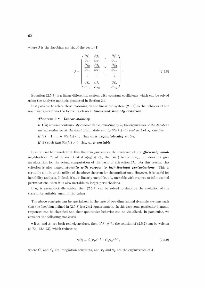
62
where J is the Jacobian matrix of the vector f :
J =
∂f1
∂u1
∂f1
∂u2· · · ∂f1
∂un
∂f2
∂u1
∂f2
∂u2· · · ∂f2
∂un...
.... . .
...
∂fn
∂u1
∂fn
∂u2· · · ∂fn
∂un
· (2.5.8)
Equation (2.5.7) is a linear differential system with constant coefficients which can be solvedusing the analytic methods presented in Section 2.4.
It is possible to relate these reasoning on the linearized system (2.5.7) to the behavior of thenonlinear system via the following classical linearized stability criterion .
Theorem 2.8 Linear stability
If f(u) is twice continuously differentiable, denoting by λi the eigenvalues of the Jacobian
matrix evaluated at the equilibrium state and by <e(λi) the real part of λi, one has:
If ∀ i = 1, . . . , n <e(λi) < 0, then ue is asymptotically stable;
If ∃ ı such that <e(λı) > 0, then ue is unstable.
It is crucial to remark that this theorem guarantees the existence of a sufficiently small
neighborhood Ie of ue such that if u(t0) ∈ Be, then u(t) tends to ue, but does not givean algorithm for the actual computation of the basin of attraction De. For this reason, thiscriterion is also named stability with respect to infinitesimal perturbations. This iscertainly a limit to the utility of the above theorem for the applications. However, it is useful forinstability analysis. Indeed, if ue is linearly unstable, i.e., unstable with respect to infinitesimalperturbations, then it is also unstable to larger perturbations.
If ue is asymptotically stable, then (2.5.7) can be solved to describe the evolution of thesystem for suitably small initial values.
The above concepts can be specialized in the case of two-dimensional dynamic systems suchthat the Jacobian defined in (2.5.8) is a 2×2 square matrix. In this case some particular dynamicresponses can be classified and their qualitative behavior can be visualized. In particular, weconsider the following two cases:
• If λ1 and λ2 are both real eigenvalues, then, if λ1 6= λ2 the solution of (2.5.7) can be writtenas Eq. (2.4.23), which reduces to:
v(t) = C1v1eλ1t + C2v2e
λ2t , (2.5.9)
where C1 and C2 are integration constants, and v1 and v2 are the eigenvectors of J.

63
Figure 2.5.1 — Qualitative behavior of the dynamic response: (a) stable, (b) unstable node.
In particular, if λ1 and λ2 are both negative, one has:
limt→+∞
v(t) = 0 , (2.5.10)
and this equilibrium point is called a stable node . On the other hand, if one of the eigenvalueis positive, it follows that:
limt→+∞
v(t) = +∞ . (2.5.11)
The equilibrium point is called an unstable node if both eigenvalues are positive and asaddle point otherwise. In this latter case, two of the trajectories meet at the equilibriumpoint and two depart from it. They are therefore called stable and unstable manifolds.
Figure 2.5.2 — Qualitative behavior of the dynamic response: (a) stable and (b) unstable focus.
• If the eigenvalues are complex conjugate, i.e., λ1 = λ + iω, λ2 = λ− iω, the solution to the

64
initial-value problem (2.5.7) can be written as in Eq. (2.4.24) by a linear combination of sineand cosine functions.
In particular, if:
λ = <e(λ1) = <e(λ2) < 0 ⇒ limt→+∞
v(t) = 0 , (2.5.12)
the equilibrium point is called a stable focus. If, instead,
λ = <e(λ1) = <e(λ2) > 0 ⇒ limt→+∞
|v(t)| = +∞ , (2.5.13)
the equilibrium point is called an unstable focus. Finally, if:
λ = <e(λ1) = <e(λ2) = 0 ,
then v(t) stays bounded and the equilibrium state is a center point .
The qualitative behavior of the solution in the case of stable and unstable node is representedin Figure 2.5.1. The qualitative behavior of the solution in the case of stable and unstable focusis represented in Figure 2.5.2.
Figure 2.5.3 — Qualitative behavior of the dynamic response: (a) saddle and (b) center point.
Finally, the qualitative behavior of the solution in the case of saddle and center point isrepresented in Figure 2.5.3.
If λ1 = λ2, the discussion gives the same results though (2.5.9) cannot be the solution of(2.5.7) as shown in (2.4.23).
Note that for n = 2 the eigenvalues of J are:
λ =trJ2±
√(trJ)2
4− detJ , (2.5.14)
where trJ = J11 + J22, and have both negative real part if and only if:
tr J < 0 and detJ > 0 . (2.5.15)

65
Example 2.5.1
Stability for the van der Pol Model
As an example, consider the van der Pol model which can for instance model the behavior ofsome nonlinear electric circuits. The mathematical model can be written as follows:
di
dt= v ,
dv
dt= (α− βi2)v − γi ,
(2.5.16)
and is characterized by a unique equilibrium given by:
v = 0 ,
(α− βi2)v + γi = 0 ,(2.5.17)
that is i = v = 0, which, according to what has just been stated, is linearly stable if α isnegative, as the Jacobian:
J(i = v = 0) =(
0 1−γ α
)(2.5.18)
has always positive determinant and trace equal to α. Hence, the equilibrium point is stable ifα < 0. More in details, the eigenvalues of the Jacobian are:
λ =12
[α±
√α2 − 4γ
], (2.5.19)
which are complex conjugate if |α| < 2√
γ, and real if |α| ≥ 2√
γ.
The stability results can be summarized in the following table:
α eigenvalues stability result
α ≤ −2√
γ real and negative stable node
−2√
γ < α < 0 complex with <e(λ) < 0 stable focus
α = 0 purely imaginary (±i√
γ) center point
0 < α < 2√
γ complex with <e(λ) > 0 unstable focus
α ≥ 2√
γ real and positive unstable node
Figure 2.5.4 — Stability analysis for the van der Pol Model

66
2.5.3 Nonlinear Stability
The linear stability criterion guarantees stability with respect to indefinitely small disturbances.To obtain this result one has to study the linear system (2.5.7), which is an approximation ofthe real model. In order to obtain more information on nonlinear stability criteria by only usingthe right-hand side of the ordinary differential equation, Liapunov suggested a method whichfor this reason is usually called Liapunov direct method . For those who are not familiar withstability theory, the method consists in finding a function, called Liapunov function , whichessentially plays the role of a generalized energy for the system. If this “energy” decreasesas the system evolves, i.e., if the system is dissipative, then the system will tend to a stableconfiguration.
Bearing this in mind, we introduce the following concept:
Liapunov function
Let ue be an isolated equilibrium of the system of equationdudt
= f(u) in some open
neighborhood De of ue. A function V = V (u) is called a Liapunov function if it
satisfies the following properties:
i) It is continuous in De and differentiable in De − ue;ii) It has a local minimum in ue, i.e., for instance:
V (ue) = 0 , V (u) > 0 for u ∈ D′e − ue
with D′e open neighborhood of ue;
iii) It is a nonincreasing function of time over any solution u(t) with initial condition
u(t0) = u0 ∈ De − ue, i.e. ∀ t ≥ t0:
dV
dt
(u(t)
)=
n∑
i=1
∂V
∂ui
dui
dt=
n∑
i=1
∂V
∂uifi
(u(t)
) ≤ 0 . (2.5.20)
Theorem 2.9 Liapunov stability
If there exists a Liapunov function V in a neighborhood De of the isolated equilibrium
state ue, then ue is stable. Furthermore, ifdV
dt
(u(t)
)< 0, then ue is also asymptotically
stable.
It is important to remark that the conditiondV
dt
(u(t)
)< 0 means that V decreases as the
system evolves. This implies that the trajectory will remain in the region delimited by thelevel curve V (u) = V (u0).
It is hard to say, in general, how to proceed to identify the best Liapunov function. For

67
instance, in the case of systems of two equations, let consider the quadratic function:
V = av21 + 2bv1v2 + v2
2 (2.5.21)
with a > b2, that is always nonnegative. Then one has to check that the sign of:
12
dV
dt=
(av1 + bv2
)f1(v1, v2) +
(bv1 + v2
)f2(v1, v2) (2.5.22)
be negative in some region near v1 = v2 = 0 for some values of a and b with a > b2.Another method is to look for V as a quadratic form V = v ·Av with A such that:
JT A + AJ = −I , (2.5.23)
where J is the Jacobian of f in v = 0, and I is the identity matrix.Liapunov Theorem 2.9 is partially inverted by the following theorem:
Theorem 2.10 Chetayev theorem
Let ue be an isolated equilibrium of du/dt = f(u) in some open set D. If there exists a
differentiable function V = V (u) and an open set D+ such that
i) ue belongs to the border ∂D+ of D+,
ii) V (u) > 0 in D+ and V (u) = 0 on ∂D+,
iii)dV
dt> 0 in D+,
then ue is unstable.
Example 2.5.2
Stability through Liapunov Method
Consider the system:
du1
dt= −u1 + u2 ,
du2
dt= u2 + 2u1u2 ,
(2.5.24)
which has u1 = u2 = 0 and u1 = u2 = −1/2 as equilibrium points. In order to check thenonlinear stability of u1 = u2 = −1/2, it is useful to introduce the perturbation (v1, v2) definedby:
u1 = −12
+ v1 , u2 = −12
+ v2 . (2.5.25)
Eq. (2.5.24) then rewrites in terms of the new variables as:
dv1
dt= −v1 + v2 ,
dv2
dt= −v1 + 2v1v2 .
(2.5.26)

68
Consider the function:
V = v21 − v1v2 +
32v22 , (2.5.27)
which is positive definite as can be written as V = v · (Av), where v = (v1, v2) and
A =
1 −12
−12
32
(2.5.28)
has both positive eigenvalues.The computation of dV/dt yields:
dV
dt= (2v1 − v2)
dv1
dt+ (3v2 − v1)
dv2
dt= −v2
1 − v22 + 6v1v
22 − 2v2
1v2 . (2.5.29)
Rewriting −v21 − v2
2 + 6v1v22 − 2v2
1v2 ≤ 0 as follows:
(2v2 + 1)v21 − 6v1v
22 + v2
2 ≥ 0 , (2.5.30)
the equality is solved by:
v1 =3v2
2 ±√
v22(9v2
2 − 2v2 − 1)2v2 + 1
· (2.5.31)
If 9v22 − 2v2 − 1 ≤ 0, that is, if
v2 ∈ I =
[1−√10
9, 1 +
√10
9
],
then (2.5.30) is always satisfied, as in I, 2v2 + 1 > 0.
2.6 Regular and Singular Perturbation Methods
As we have already seen, mathematical models must always be written in terms of suitable di-mensionless variables. This technical manipulation may generate dimensionless numbers whichare small with respect to unity, while the independent and dependent variables are of the orderof unity. Almost always, these parameters have a well defined physical meaning which shouldbe related to the solution of mathematical problems (or vice versa).
This section provides a brief introduction to regular and singular perturbation methods bymeans of simple examples where the dependent variable is a scalar or a two dimension vector.
We first define a perturbed model. Let ε be a positive number which is small with respectto unity.

69
Regularly Perturbed Model
A finite mathematical model:
du
dt= f(t, u, ε) ,
u(t0, ε) = u0(ε) .
(2.6.1)
is called regularly perturbed if f(t, u, ε) and u0(ε) depend smoothly on their argu-
ments.
Singularly Perturbed Model
A finite mathematical model is called singularly perturbed if it can be written as
εdu
dt= f(t, u) ,
u(t0, ε) = u0(ε) .
(2.6.2)
The above definitions are given for a scalar problem. Their generalization to systems ofequations requires technical additional calculations..
As it is shown in the examples which follow, the parameter ε (in a regularly perturbedproblem) is linked to the presence in the model of nearly negligible physical phenomena, whilein a singularly perturbed problem the parameter ε is generally related to the scaling and to thedimensional analysis of the variables.
Different methods have to be developed for each of the above classes of models, as it willbe shown in the next subsections. The starting point is the idea of looking for an asymptoticexpansion, in the sense of Poincare, for ε → 0, uniformly valid in an interval [t0, T ], for thesolution u(t, ε) of the perturbed problem, and we write:
u(t, ε) ∼∞∑
i=0
ui(t)εi as ε → 0 . (2.6.3)
This means that there exists a positive constant ε0 and that ∀N ≥ 0, there exist functionsui(t)N
i=0 defined in [t0, T ], and a positive constant KN such that:
∣∣∣u(t, ε)−∑Ni=0 ui(t)εi
εN+1
∣∣∣ < KN , (2.6.4)
for all ε ∈ (0, ε0) and for all t ∈ [t0, T ].
Using the Landau symbol “O”, condition (2.6.4) can be written:
u(t, ε) =N∑
i=0
ui(t)εi + O(εN+1) as ε → 0 , (2.6.5)
70
uniformly valid for t ∈ [t0, T ]. The series on the right-hand side of (2.6.3) is called asymptot-ically convergent, uniformly in [t0, T ]. The concepts of convergent series and asymptoticallyconvergent series are quite different: we refer to De Jager and Furu (1996) for a discussionabout convergence versus asymptotic convergence.
Starting from the above preliminaries it is shown in the next subsection how to deal with therelatively simpler case of regular perturbations. Subsequently the case of singular perturbedproblems is considered.
2.6.1 Regular perturbation method for initial value problems
Let us consider the regularly perturbed problem (2.6.1) and let us define as limiting problemassociated to (2.6.1) the initial value problem obtained from (2.6.1) for ε = 0:
du(0)
dt= f(t, u(0), 0) ,
u(0)(t0, 0) = u0(0) .
(2.6.6)
Due to the smoothness of f(t, u, ε) and u0(ε) with respect to their arguments, we espect thatthe solution u(t, ε) of (2.6.1) depends smoothly on t and ε and that it tends to the solutionu(0)(t) of the limiting problem (2.6.6), as ε → 0, uniformly with respect to t ∈ [t0, T ].
Following De Jager and Furu (1996), let us assume that f(t, u, ε), defined on IR2 × [0, 1], hasthe following expansion:
f(t, u, ε) ∼∞∑
i=0
f (i)(t, u)εi as ε → 0 , (2.6.7)
uniformly valid in any bounded domain of IR2, with the functions f (i)(t, u) infinitely differen-tiable in IR2, and assume that:
u0(ε) ∼∞∑
i=0
u0iεi . (2.6.8)
Then, let us look for an asymptotic expansion for the solution of problem (2.6.1):
u(t, ε) ∼∞∑
i=0
u(i)(t)εi , (2.6.9)
along the following steps:
Step 1. Substituting (2.6.9) in (2.6.7), yields:
f(t, u(t, ε), ε) ∼∞∑
i=0
εi f (i)(t,
∞∑
j=0
u(j)(t)εj)
∼∞∑
i=0
εi
f (i)(t, u(0)(t)) +∂f (i)
∂u(t, u(0)(t))
∞∑
j=1
u(j)(t)εj
71
+12
∂2f (i)
∂u2(t, u(0)(t))
( ∞∑
j=1
u(j)(t)εj)2
+ · · ·
=f (0)(t, u(0)(t)) + ε∂f (0)
∂u(t, u(0)(t))u(1)(t)
+ f (1)(t, u(0)(t))
+ ε2∂f (0)
∂u(t, u(0)(t))u(2)(t)
+12
∂2f (0)
∂u2(t, u(0)(t))(u(1)(t))2 +
∂f (1)
∂u(t, u(0)(t))u(1)(t)
+ f (2)(t, u(0)(t))
+ · · ·+ εp∂f (0)
∂u(t, u(0)(t))u(p)(t)
+ f (p)(t, u(0)(t), u(1)(t), · · · , u(p−1)(t))
+ · · · , (2.6.10)
with f (p) are known functions depending only on (t, u(0), u(1), · · · , u(p−1)).
Step 2. Consider from Step 1, that:
f(t, u(t, ε), ε) ∼ f (0)(t, u(0)(t)) +∞∑
i=1
εi∂f (0)
∂u(t, u(0)(t))u(i)(t)
+ f (i)(t, u(0)(t), u(1)(t), · · · , u(i−1)(t))
, (2.6.11)
then substituting (2.6.11), (2.6.9) and (2.6.8) into the corresponding terms of problem (2.6.1),and equating the same powers of ε, the following systems are obtained:
du(0)
dt= f (0)(t, u(0)) ,
u(0)(t0) = u00 ,
(2.6.12)
and
du(i)
dt=
∂f (0)
∂u(t, u(0))u(i) + f (i−1)(t, u(0), u(1) · · · , u(i−1)) ,
u(i)(t0) = u0i ,
(2.6.13)
for i = 1, 2, . . . .
Step 3. Applying to problem (2.6.12) the existence and uniqueness Theorems 2.1-2.2, weget the existence of a unique solution u(0)(t) of (2.6.12), for t ∈ [t0, T ]. Recalling that f (0)(t, u)is infinitely differentiable, the solution u(0) is C∞. Moreover, referring to subsection 2.4.2, thesolutions of the linear differential systems (2.6.13) in the same interval [t0, T ] is obtained.
Step 4. The procedure has to be completed showing that the formal expansion (2.6.9) foru(t, ε), where the terms u(i)(t) are the solutions of systems (2.6.12) and (2.6.13) obtained in
72
Step 3, is an asymptotic expansion for u(t, ε). This means that, writing ∀N ≥ 0,
u(t, ε) =N∑
i=0
u(i)(t)εi + RN (t, ε) , (2.6.14)
it has to be proved that:
RN (t, ε) = O(εN+1) , (2.6.15)
uniformly in t ∈ [t0, T ]. The reader is addressed to O’Malley (1991) or De Jager and Furu(1996) for the details of this proof.
Remark 2.6.1. The precedure described in Step 1 - Step 4 refers to the scalar problem (2.6.1).
In the general case of a system of equations, the method of looking for an asymptotic expansion
for the solution of the system can also be applied, as it is shown in the following example from
Humi and Miller (1988).
Example 2.6.1
Consider the system:
du
dt= −2u + v + εv2 ,
dv
dt= u− 2v + εu2 ,
u(0) = v(0) = 1 ,
(2.6.16)
and the perturbation expansions for u and v:
u(t, ε) ∼∞∑
i=0
u(i)(t)εi , v(t, ε) ∼∞∑
i=0
v(i)(t)εi . (2.6.17)
Appling the perturbation method outlined above, we obtain at order i = 0 and i = 1,respectively:
du(0)
dt= −2u(0) + v(0) ,
dv(0)
dt= u(0) − 2v(0) ,
u(0)(0) = v(0)(0) = 1 ,
(2.6.18)
and
du(1)
dt= −2u(1) + v(1) + (v(0))2 ,
dv(1)
dt= u(1) − 2v(1) + (u(0))2 ,
u(1)(0) = v(1)(0) = 0 .
(2.6.19)
73
We may observe that (2.6.16) is symmetric in u, v, as well as (2.6.18) and (2.6.19) are sym-metric in u(0), v(0) and u(1), v(1) respectively. Solving the linear systems (2.6.18) and (2.6.19)yields:
u(0)(t) = v(0)(t) = e−t , u(1)(t) = v(1)(t) = e−t − e−2t , (2.6.20)
that gives as solution of (2.6.16):
u(t, ε) = v(t, ε) = e−t + ε(e−t − e−2t) + O(ε2) . (2.6.21)
Example 2.6.2
Duffing’s Equation - Part I
Let consider the following system related to the motion of a mass attached to a nonlinear spring(hard spring):
d2u
dt2+ u + εu3 = 0 ,
u(0) = a ,du
dt
∣∣∣∣t=0
= 0 ,
(2.6.22)
where ε ∈ (0, 1), which can be considered as a regular perturbation of
d2u
dt2+ u = 0 ,
u(0) = a ,du
dt
∣∣∣∣t=0
= 0 .
(2.6.23)
Problem (2.6.22) is equivalent to the following two-dimensional first order system:
du
dt= v ,
dv
dt= −u− εu3 ,
u(0) = a , v(0) = 0 .
(2.6.24)
The power series expansion method gives at order i = 0 and i = 1 the following systems:
d2u(0)
dt2+ u(0) = 0 ,
u(0)(0) = a ,du(0)
dt
∣∣∣∣t=0
= 0 ,
(2.6.25)

74
and
d2u(1)
dt2+ u(1) = −(u(0))3 ,
u(1)(0) = 0 ,du(1)
dt
∣∣∣∣t=0
= 0 ,
(2.6.26)
where (2.6.25) is solved by u(0)(t) = a cos t , so that system (2.6.26) for u(1) can be written asfollows:
d2u(1)
dt2+ u(1) = −a3
(14
cos 3t +34
cos t
),
u(1)(0) = 0 ,du(1)
dt
∣∣∣∣t=0
= 0 .
(2.6.27)
Its solution is:
u(1)(t) = a3
[132
(cos 3t− cos t
)− 3
8t sin t
], (2.6.28)
so that the solution of (2.6.22) can be written as follows:
u(t, ε) = a cos t + εa3
[132
(cos 3t− cos t
)− 3
8t sin t
]+ O(ε2) , (2.6.29)
uniformly in any bounded interval 0 < t < T .
Remark 2.6.2. It is interesting to remark that we do not get any answer to the question of
how big can be the deviation of the solution of problem (2.6.1) from the solution of problem
(2.6.6) on a large time interval. The following simple examples show that this deviation may
even be not small.
Example 2.6.3
Let consider the scalar system, from Mishchenko and Rozov (1980),
du
dt= (u + ε)2 ,
u(0) = 0 ,
(2.6.30)
that for ε = 0 becomes:
du
dt= u2 ,
u(0) = 0 .
(2.6.31)
The solution of (2.6.31) is u(t) = 0, ∀ t ∈ [0,∞), while the solution of (2.6.30) is u(t, ε) =ε
1− εt− ε and it is defined only for t ∈ [0, 1/ε).
75
Example 2.6.4
Lindstedt-Poincare Algorithms
Coming back to Example 2.6.2, we see that expression (2.6.29) is a reasonable approximationof the solution for bounded time intervals but not for t ∈ [0,∞). In fact due to the term−(3/8) t sin t in (2.6.29), when t = O(1/ε) the second term of the expansion is no longer O(ε)and when t = O(1/ε2) the second term blows up.
Let us notice here that the term −(3/8) t sin t in (2.6.29) is due to the presence of the term−(3/4)a3 cos t in (2.6.27) (the so–called resonance effect). On the other hand, (2.6.22) hasonly bounded (and periodic) solutions, as it describes a conservative system with the energyintegral:
(du
dt
)2
+ u2 +ε
2u4 = a2 +
ε
2a4 , (2.6.32)
which implies u and du/dt are bounded for t ∈ [0,∞).This suggests to use a different expansion of the solution in which unbounded terms do not
appear: a possible approach is the Lindstedt-Poincare algorithm.Let s be a new variable defined as follows:
t = s ω(ε) , (2.6.33)
where
ω(ε) = 1 + εω1 + ε2ω2 + · · · . (2.6.34)
System (2.6.22) can now be written in the unknown u(s) = u(t(s)) as:
d2u
ds2+ (1 + εω1 + ε2ω2 + · · ·)2(u + εu3) = 0 ,
u(0) = a ,du
ds
∣∣∣∣s=0
= 0 .
(2.6.35)
The above procedure can be applied to this problem looking for an asymptotic power seriesexpansions for the solution of the type:
u(s, ε) ∼∞∑
i=0
u(i)(s)εi . (2.6.36)
The power series expansion method gives, respectively to the order i = 0, 1, 2, the followingsystems:
d2u(0)
ds2+ u(0) = 0 ,
u(0)(0) = a ,du(0)
ds
∣∣∣∣s=0
= 0 ,
(2.6.37)

76
d2u(1)
ds2+ u(1) = −(u(0))3 − 2ω1u
(0) ,
u(1)(0) = 0 ,du(1)
ds
∣∣∣∣s=0
= 0 ,
(2.6.38)
d2u(2)
dt2+ u(2) = −3(u(0))2u(1) − 2ω1(u(1) + (u(0))3)
− (ω12 + 2ω2)u(0) ,
u(2)(0) = 0 ,du(2)
ds
∣∣∣∣s=0
= 0 .
(2.6.39)
The solution of (2.6.37) is u(0)(s) = a cos s, so that system (2.6.38) for u(1) can be rewrittenas follows:
d2u(1)
ds2+ u(1) = −1
4a3 cos(3s)−
(34a2 + 2ω1
)a cos s ,
u(1)(0) = 0 ,du(1)
ds
∣∣∣∣s=0
= 0 ,
(2.6.40)
so that, we can choose ω1 such that:
34a2 + 2ω1 = 0 , (2.6.41)
in order to avoid the resonance effect. Therefore, the following bounded solution of (2.6.37) isobtained:
u(1)(s) =132
a3 (cos 3s− cos s) . (2.6.42)
Consequently,
u(s, ε) = a cos s +132
a3 (cos 3s− cos s)ε + O(ε2) , (2.6.43)
that is uniformly valid in any finite s interval, with the coordinate s given by:
s = t ω(ε)−1 = t(1− 3
8a2ε + · · ·
)−1
. (2.6.44)
Finally the solution of (2.6.22) can be written as follows:
u(t, ε) = a cos(Ωt) +ε
32a3(cos(3Ωt)− cos(Ωt)) + O(ε2) , (2.6.45)
where
Ω = ω(ε)−1 =(1− 3
8a2ε + · · ·
)−1
= 1 +38a2ε + O(ε2) . (2.6.46)
77
2.6.2 Singularly perturbed problems
As we have seen in the preceding subsection, in the case of regularly perturbed problem (2.6.1),the solution depends on the parameter ε in such a way that the solution u(t, ε) converges,as ε → 0, to the solution u(0)(t) of the limiting problem (2.6.6), uniformly with respect tot ∈ [t0, T ]. On the other hand, in the case of the singularly perturbed problem (2.6.2), theconvergence u(t, ε) → u(0)(t) generally fails. Let us introduce some basic notions and definitionsthrough the following examples.
Example 2.6.5
Initial Layer Effect - First Order Problem
Let us consider the problem:
εdu
dt+ u = 1 ,
u(0) = u0 ,
(2.6.47)
which has the unique solution:
u(t, ε) = 1 + (u0 − 1)e−tε , ∀ t > 0 . (2.6.48)
Assuming ε > 0 and u0 6= 1 yields:
limε→0+
u(t, ε) = 1 for t > 0 , u(0, ε) = u0 , (2.6.49)
that proves that the convergence of u(t, ε) to 1, for ε → 0+, is not uniform in any right-neighbourhood of t = 0.
Remark 2.6.3. The solution (2.6.48) of system (2.6.47) is the sum of two terms: the first one,
the outer or bulk solution, is an asymptotic solution of the differential equation for t > 0,
and the second one, the initial layer solution, is a function of what is called stretched time
variable:
τ =t
ε· (2.6.50)
As τ → +∞, the initial layer solution is decreasing to zero. The stretched time can be considered
as a rescaling parameter which magnifies the region of non-uniform convergence.
Example 2.6.6
Initial Layer Effect - Second Order Problem
Let us now consider the following nonlinear second order boundary value problem:
εd2u
dt2=
(du
dt
)2
,
u(0) = 1 , u(1) = 0 ,
(2.6.51)
78
which is solved by:
u(t, ε) = −ε log(t + e−
1ε (1− t)
), for t ∈ [0, 1] and ε > 0 . (2.6.52)
As in the preceding example, we have:
limε→0+
u(t, ε) = 0 , u(0, ε) = 1 , (2.6.53)
which shows that the convergence u(t, ε) → 0 for ε → 0 is uniform to respect to t on each closedsubinterval of (0, 1], but not in [0, 1].
Different solution techniques can be applied to solve and to overcome the problem of non-uniform convergence both for singularly perturbed initial value problems and for singularlyperturbed boundary value problems. Here we limit ourselves to show in the following exampleof singularly perturbed boundary value problem how an asymptotic expansion technique canbe applied.
Example 2.6.8
Friedrichs’ Problem
Consider the following second order linear boundary value problem:
εd2u
dt2+
du
dt+ u = 0 ,
u(0) = a , u(1) = b ,
(2.6.54)
for t ∈ [0, 1] and ε ∈ (0, 1), whose exact solution is:
u(t, ε) =(aes2 − b)es1t + (b− aes1)es2t
es2 − es1, (2.6.55)
with s1,2 =−1±√1− 4ε
2ε.
Assume now that we don’t know the exact solution and we want to try to determine anasymptotic form of the solution of (2.6.54) writing:
u(t, ε) = U(t, ε) + u(τ, ε) , (2.6.56)
where τ =t
ε.
Referring to the definitions stated in Remark 2.6.3, U(t, ε) represents the outer solution andu(τ, ε) the initial layer solution. Let us assume that the following power series expansion holds:
U(t, ε) ∼∞∑
i=0
U (i)(t)εi , u(τ, ε) ∼∞∑
i=0
u(i)(τ)εi . (2.6.57)

79
and assume that u(i) and its derivatives tend to zero as τ → +∞, providing the desired resultthat the correction term u has only a significant value in a neighbourhood of t = 0. The outersolution U has to solve:
εd2U
dt2+
dU
dt+ U = 0 ,
U(1, ε) = b .
(2.6.58)
The expansion gives the following first order linear problems defined inductively:
dU (0)
dt+ U (0) = 0 , U (0)(1) = b , (2.6.59)
dU (i)
dt+ U (i) = −d2U (i−1)
dt2, U (i)(1) = 0 i = 1, 2, . . . . (2.6.60)
Solving the related problems gives:
U(t, ε) = be1−t + εb(1− t)e1−t + O(ε2) , (2.6.61)
which is asymptotically valid for t ∈ (0, 1]. For t = 0 we have:
U(0, ε) = be + εbe + O(ε2) 6= a , (2.6.62)
which shows that for taking into account the initial condition, the initial layer correction u mustbe considered. The problem for u is the following linear homogeneous one:
d2u
dτ2+
du
dτ+ εu = 0 , u(0, ε) = a− U(0, ε) . (2.6.63)
The expansion for u gives at order i = 0:
du(0)
dτ+ u(0) = 0 , u(0)(0) = a− U (0)(0) = a− be . (2.6.64)
which is solved by:
u(0)(τ) = (a− be) e−τ . (2.6.65)
So we have shown that Problem (2.6.54) has the following unique asymptotic solution:
u(t, ε) = U (0)(t) + u(0)( t
ε
)+ O(ε) = b e1−t + (a− be) e−
tε + O(ε) . (2.6.66)
It is worth stressing that u(0, ε) = a, and for ε > 0 we have u(1, ε) = b + (a − be) e−1ε and
u(1, ε) → b as ε → 0+.

80
The algorithm shown in Example 2.6.8 can also be applied to the initial value problem foran autonomous system of differential equations in the form:
εdu
dt= f(u, v) ,
dv
dt= g(u, v) ,
u(0) = µ(ε) , v(0) = η(ε) ,
(2.6.67)
where u and v can be scalar or vector functions of t, and the dimensions of u and v can bedifferent.
Implementing such an algorithm from a numerical point of view, as reported in Mika andPalczewski (1991), means to solve a number of equations equal to the order of approximationplus one. In this paper, the authors propose a different algorithm which involves only onedifferential equation for a single function. This algorithm is here briefly illustrated in thefollowing example, while the reader is addressed to the original paper for the details.
Example 2.6.9
Mika and Palczewski’s Algorithm
Consider the boundary value problem:
εd2u
dt2+
du
dt+ u2 = 0 ,
u(0) = η ,du
dt
∣∣∣∣t=0
= µ ,
(2.6.68)
which corresponds to the system:
εdu1
dt= −u1 − u2
2 ,
du2
dt= u1
u1(0) = µ , u2(0) = η .
(2.6.69)
The algorithm leads, as first order approximation, to solve the following system:
εdw
dt= −w2 − 2εw2 ,
w(0) = η + ε(µ + η2) ,
(2.6.70)
and it is possible to prove that the accuracy obtained in this new algorithm is similar to thatfor the first order standard algorithm and much better than the zero order standard algorithm.
81
2.7 Bifurcation and Chaotic Motions
This section focus on how the equilibrium configurations of a dynamical system usually dependon the parameters which characterize the model. In particular, it may occur that as oneof the parameters crosses a critical value, the solution will tend toward another equilibriumconfiguration. The aim of this Section is to give some hints for the study of the bifurcation ofa dynamical system without claiming any completeness on the treatment of the subject. For adetailed treatment of the subject, refer for instance to the book Bellomo et al. (2000).
Consider a mathematical model described by a scalar autonomous ordinary differential equa-tion depending on a parameter α:
du
dt= f(u;α) . (2.7.1)
The equilibrium configurations are determined by solving the algebraic equation:
f(u; α) = 0 . (2.7.2)
This equation is usually nonlinear and for each value of α it can be solved by a certain numberof values of u, or possibly by no value at all. The number of solutions of (2.7.2) cannot bedetermined a priori and generally changes with α. As will be shown later in this section, thevalues of α for which the number of solutions of (2.7.2) changes are particularly important inthe stability analysis.
Then, one can represent by dots in the (u, α)-plane, the solutions of (2.7.2) obtained for eachfixed value of α. If α varies continuously, the solution of (2.7.2) defines a certain number ofcurves, each of which can be locally described by an equation u = ue(α), implicitly defined by(2.7.2), i.e., such that f(ue(α); α) = 0.
If one is able to determine the stability property of each equilibrium configuration, thenthis piece of information can also be reported on the diagrams using the following classicalconvention:
• Stable equilibrium configurations are identified by a heavy solid line;
• Unstable equilibrium configurations are identified by a dashed line.
The figures obtained by drawing these curves are called stability diagrams, (or bifurcationdiagrams, branching diagrams, response diagrams), and each of the curves appearing in thediagram is called a branch.
The generalization of the above considerations, given for the scalar case, to systems of equa-tions is technical.
The following definitions are recalled:
Branch points
The values(α,ue(α)
)where the number of equilibrium solutions changes are called
branch points.

82
Bifurcation points
An equilibrium solution bifurcates from another at α = αb if there are two distinct
branches ue(α) and ue(α) continuous in α, such that ue(αb) = ue(αb). The common
value(αb, ue(αb)
)=
(αb, ue(αb)
)in the (α,u)-space is called a bifurcation point.
Not all branch points are, however, bifurcation points. That is, not all changes in the numberof equilibrium solutions are due to the intersection of curves in the stability diagram. Bi-furcation points can be further classified, e.g. pitchfork bifurcation, supercritical, subcriticaland transcritical bifurcations and Hopf bifurcations, referring again to the book Bellomo et al.
(2000) for details. The following definitions can be reported:
Pitchfork bifurcation
If one of the two branches intersecting at the bifurcation point (αb,ub) is one sided
(i.e., defined only for α ≥ αb or for α ≤ αb), then the bifurcation is of the pitchfork
type.
Supercritical and subcritical bifurcations
A pitchfork bifurcation is defined as being supercritical if the one-sided branch is
stable and is otherwise subcritical .
Transcritical bifurcations
A bifurcation is transcritical if on both sides of the bifurcation point there are
locally two equilibrium solutions.
In many applications it may happen that, still departing from an unstable configuration,the system will neither go to another stationary configuration nor wander away, but will startoscillating approaching a periodic orbit. The oscillations described here are also referred to inmechanics as self-sustained oscillations, to distinguish them from those which are due tooscillatory forcing terms. One can then state the following definition:
Limit cycle
An orbit u(t) tends to a closed curve Γ called the limit cycle if there exists a period
T > 0 such that the sequence of points u(t+nT ) tends to a point of Γ as the integer
n goes to infinity.
A cycle Γ is asymptotically stable if there exists a neighborhood UΓ of Γ such that if
u(0) ∈ UΓ, then u(t) tends to Γ.
The relevance of limit cycles is basically related to the problem of how time-periodic behaviorsmay arise from the bifurcation of a steady state. This is an interesting problem in the case ofsystems of equations, i.e. in the case of dimension more than one. In fact, for a scalar problem(2.7.1), it is impossible to have a nonconstant periodic solution.
83
The behavior of a dynamical system may change, according to the value assumed by a pa-rameter α and the solution will tend to a time periodic orbit, as a critical value αb is crossed.In this case, the bifurcation is called the Hopf bifurcation.
The identification of self-sustained oscillations is far more difficult than that of equilibriumpoints. As a consequence, recognizing the existence of a Hopf bifurcation can be a hard task.In this respect, the following theorem, known as the Hopf Theorem, is often very helpful.
Theorem 2.11 Hopf Theorem
Focussing on the dependence of the equilibrium configuration ue on a parameter α, let
us assume that there is a critical value αb, such that ue(α) is asymptotically stable for
α < αb and unstable for α > αb. If for α = αb the Jacobian J of f has a simple pair of
purely imaginary eigenvalues:
λ(αb) = ± iΩ , (2.7.3a)
and all the other eigenvalues have a negative real part and, furthermore, for α close to
αb:
λ(α) = µ(α)± iω(α) , withdµ
dα(α = αb) > 0 . (2.7.3b)
Therefore for α sufficiently near the critical value αb, there exists a limit cycle with initial
period:
T =2π
Ω· (2.7.3c)
If, in addition, the equilibrium configuration u(α = αb) is locally asymptotically stable,
then the limit cycle is stable.
The theorem above uses again the eigenvalues of the Jacobian and the knowledge of thestability properties which are not too hard to verify. In particular, it pays attention to whathappens to the first eigenvalue which will have positive real part as the bifurcation value iscrossed.
We already know that at criticality. i.e. for α equal to the critical value αb, the real partof an eigenvalue or of a pair of eigenvalues vanishes and becomes positive as the bifurcationvalue is passed by, while that of the others is negative. The theorem states that if also theimaginary part vanishes, i.e., the eigenvalue is zero, then the bifurcation involves stationaryconfigurations. If, instead, there is a pair of purely imaginary eigenvalues, then the bifurcationinvolves self-sustained oscillations. This situation is represented in Figure 2.7.1. In particular,in Figure 2.7.1b a pair of eigenvalues of J crosses the imaginary axis from left to right awayfrom the origin as α, increasing from stable values to unstable ones, crosses criticality.
Generally, the Hopf theorem does not tell whether a stable (supercritical) limit cycle exists forα > αb or an unstable (subcritical) limit cycle exists for α < αb, inside of which all orbits spiraltoward ue and outside of which the orbits diverge. In order to know whether the limit cycle is

84
Figure 2.7.1 — Behavior of the critical eigenvalues as α increases from stable values to unstableones in the case of (a) stationary bifurcation and (b) Hopf bifurcation.
stable or unstable, it must be proved that ue is locally asymptotically stable at criticality. Thisinformation can be achieved by using the Liapunov method. In fact, linear stability criteriaare useless because at criticality the eigenvalues are purely imaginary. This precludes anyconclusion on the character of the nonlinear system. This second part is, however, certainlynot simple.
These concepts are now applied to the following example.
Example 2.7.1
Limit Cycle for the van der Pol Model
Consider the van der Pol equation already encountered in Example 2.5.1:
d2u
dt2− (α− βu2)
du
dt+ u = 0 , (2.7.4)
with β > 0 and, without loss of generality, γ = 1.
The only equilibrium configuration is u = 0, which is asymptotically stable for α < 0 andunstable for α > 0. In fact, the eigenvalues of the Jacobian are:
λ =α±√α2 − 4
2·
Therefore, near the origin µ = <e(λ) = α/2. Furthermore, at criticality,
λ(α = 0) = ± i 6= 0 anddµ
dα(α = 0) =
12
> 0 .
From Hopf theorem, then, there exists a limit cycle. To establish if the limit cycle is subcritical(unstable) or supercritical (stable), one has to verify that u = 0 is locally asymptotically stablefor α = 0.

85
By using V = u2 +(
du
dt
)2
as a Liapunov function, one can compute for α = 0,
dV
dt= −βu2
(du
dt
)2
, (2.7.5)
which is always negative for non-trivial solutions.
2.8 Critical Analysis
An introduction to mathematical modelling at the microscopic scale has been given in thischapter focusing on models stated in terms of ordinary differential equations. It has beenshown that the analysis of nonlinear systems needs to be approached using both analytic andcomputational schemes. Analytic methods can provide existence results and some informationon the qualitative behavior of the solution, for instance stability properties, asymptotic be-havior, bifurcations, while computational schemes integrate the information by visualizing andcompleting what found by analytic methods.
Generally, none of the two approaches, namely analytic and computational, is sufficient todeliver a complete information, while a sinergetic use can be successful in providing a picture,as complete as possible of the solution patterns. Simulations, based on computational schemes,have to be focussed on completing, and possible enlarging, what is delivered (and not delivered)by the analytic qualitative analysis.
Let us analyze some modeling and complexity issues related to the contents of this chapter.Finite models, i.e. at the microscopic scale, consider each system as a whole. It is worthreasoning about some implications of the above approximation of physical reality. In fact, thisapproximation can be, in some cases, not acceptable when the number of elements constitutingthe overall system under consideration is large, namely the number of ordinary differentialequations to be dealt with is too high for the qualitative analysis, as well as for computationaltreatment.
Moreover, let us critically consider that all models we have seen in this chapter need pa-rameters related to the material behavior of the system under consideration. For instance,elasticity characteristics of spring, coefficients of competitive and/or cooperative models, andso on. Generally, these parameters are measured by empirical data obtained near equilibrium,while their values are needed to describe the evolution of the system far from equilibrium.
Finally, let us observe that most of the models presented in this chapter belong to the inertmatter. Therefore they do not take into account the ability of living systems to extract energyfrom the outer environment and live out of equilibrium. Moreover, the deterministic causalityprinciples, which are valid for models of the inert matter, should be replaced by relations wherethe effect is related to the cause only in some probabilistic sense.

86
This aspect is even more difficult to treat in the case of large systems where, as in most livingsystems, interactions are not linearly additive. This chapter has skipped over all aforesaidproblems which will be treated later in Chapter 4, by mathematical tools that appear to beappropriate to take into account all topics outlined in this section.

87
Chapter 3
Macroscopic Scale Modelsand Partial Differential Equations
3.1 Introduction
This chapter deals with the derivation and analysis of mathematical models derived at themacroscopic scale. These models, according to the definitions given in Chapter 1, providea description of real systems by suitable evolution equations for locally averaged quantitieswhich can be called macroscopic observable quantities. Of course, all physical systemsare constituted by several interacting elements. However, the local averaging is an acceptableapproximation when a small volume, in terms to be still precisely defined, contains a sufficientlylarge number of elements.
The above approximation can be called continuous matter assumption, which states thatgiven two points belonging to the system, however close each other, some matter is includedbetween these points. A typical example is the flow of fluid particles regarded as a continuumsystem. Rather than modelling the dynamics of each single particle and then averaging to obtaingross quantities such as mass density and linear momentum, the macroscopic approach providesdirectly, as we shall see, the evolution in time and space of the above macroscopic quantities.This approach was already analyzed in Chapter 1, where a few introductory examples havealso been proposed. Therefore we simply recall that the derivation of equations in continuumphysics has been a fundamental chapter in the history of mathematical physics and, in general,in the history of sciences.
Models of continuum physics, e.g. fluid dynamics, elasticity, electromagnetism fields, havebeen derived at the macroscopic scale under the continuum matter approximation, and arenowadays the fundamental background of the mathematical models of natural, applied, andtechnological sciences. Moreover, the derivation of several models in technology takes advantageof the above fundamental models of mathematical physics.
As we have already seen in Chapter 1, macroscopic models are characterized by a statevariable u which depends on time and space. In general this dependence is continuous and one

88
can write
u = u(t,x) : [0, T ]×D 7−→ IRn , (3.1.1)
where D ⊆ IR3 is the domain of the space variable and u is an n-dimensional vector. Math-ematical models are generally stated in terms of a system of partial differential equations forthe variable u.
If the state variable is a scalar and the space variable is in dimension one, then one simplyhas
u = u(t, x) : [0, T ]× [a, b] 7−→ IR . (3.1.2)
In this case the model is a scalar partial differential equation.
Static continuous models are such that the dependence on time drops and the state variableis
u = u(x) : D 7−→ IRn . (3.1.3)
The organization of this chapter is somehow analogous to the one of the previous one. Afterthe above introduction, the contents are organized as follows:
– Section 3.2 deals first with the description of some general modelling methods; then, thesemethods are will be applied to the derivation of some elementary models of mathematicalphysics related to simple phenomena, such as wave propagation, thermal diffusion.
– Section 3.3 analyzes the contents of the preceding section and deals with a classification ofmodels and equations. This means looking at the mathematical structure of the models toprovide a classification based on common properties of the said equations. As we shall see, theclassification, based on mathematical properties, can be related to different classes of physicalphenomena described by the model.
– Section 3.4 deals, on the basis of the above classification, with the statement of mathemat-ical problems. The above classification is finalized to the correct statement of mathematicalproblems technically related to the development of mathematical methods. The mathematicalformulation of problems is, as we shall see, preliminary to their solution and to the developmentof simulations.
– Section 3.5 deals with an introduction to analytic methods for linear problems. It is only abrief introduction considering that these Lecture Notes are mainly devoted to nonlinear modelsand problems, a relatively deeper insight can be obtained by the pertinent literature which willbe given in what follows.
– Section 3.6 deals with the discretization of continuous models into a discrete number of finitemodels. Using this method, one obtains a set of models which approximate the continuous oneby a system of ordinary differential equations related to the evolution of each finite element.
– Section 3.7 proposes a critical analysis mainly focused on the selection of the macroscopicscale to represent the system.

89
It is worth mentioning that this chapter does not aim to provide a complete presentation ofthe large variety of models of mathematical physics. The aim is to deal with methodologicalaspects which may contribute to address the reader to mathematical modelling as a science.The examples of models proposed in this chapter have to be regarded as relatively simple onesproposed as a mathematical description of simple phenomena.
3.2 Modelling Methods and Applications
This section deals with the analysis of the methodological aspects of the mathematical mod-elling of continuous systems, which will be then applied to the study of a number of physicalsystems chosen as suitable examples.
As usual, the derivation of a mathematical model suitable to describe a certain physicalsystem requires a preliminary phenomenological observation both of the physical system andof its connection with the outer environment. Then, the modelling procedure can be developedalong the following steps:
1: Selection of the state variable which describes, by the model, the real system: this variablecan be called state variable;
2: Modelling of the interactions between the inner system under consideration and the outerenvironment;
3: Assessment of the equilibrium, conservation, and/or balance equations, related to the abovedefined state variable, including the action of the outer environment to the inner system.
4: Modelling the material behavior of the system by means of phenomenological models, whichwill be called constitutive or material models;
5: Derivation, using the equations dealt with in Steps 3 and 4, of a mathematical model. Suchmodel consists of a suitable set of equations describing in time and space the evolution of thestate variable.
The above scheme does not claim to cover all conceivable types of modelling procedures.However, various examples are proposed to the reader to achieve a general understanding ofthe above methodology and of its generalization.
Then, once the mathematical model has been designed, the usual procedure for its analysiscan be organized: formulation of mathematical problems by a proper statement of initial andboundary conditions, qualitative analysis, solution of mathematical problems, and validationof the model.
As mentioned in Step 3, several methodological approaches can be followed toward the deriva-tion of a certain model, while a common feature of the analysis developed in what follows isthat we consider a real system represented with reference to a certain fixed, generally inertial,frame.
Moreover, models are derived under the assumption that the matter is continuous. This iscertainly an approximation, since intermolecular distances are always positive quantities. On

90
the other hand, when these distances are sufficiently small with respect to the characteristicdimensions of the body, the continuum hypothesis becomes reasonable and can be regarded asan acceptable simplification. If this hypothesis is no longer applicable, for instance for a rarefiedgas, then mathematical models have to be derived at a molecular scale, as we shall see in thenext chapter.
Some examples of models and of the related modelling techniques will be now given in whatfollows.
Example 3.2.1
Modelling the Vibration of an Elastic String
Let us consider, with reference to Fig. 3.2.1, an elastic string fixed at both its extrema. Themodelling procedure for the dynamics of the system can be based upon the following assump-tions:
• The string is held in A and B by a strong tension directed along the string. This implies thatgravity can be neglected, and that consequently the string takes at equilibrium a straightconfiguration, identified by the axis with unit vector i.
• The string is subjected to small displacements from the equilibrium configuration.
• The motion of the string is localized on a plane, identified by the unit vectors i and j andevery point of the string moves along j, namely perpendicularly to the equilibrium state.
• The state variable is the perpendicular displacement
u = u(t, x) : [0, T ]× [0, `] 7−→ IR , (3.2.1)
where the independent variables are time t and location x along the string.
• A fluid-dynamic drag is exerted on the string by the outer environment. A phenomenologicalmodel of the force acting upon the string element ∆x is as follows
F = −h
∣∣∣∣∂u
∂t
∣∣∣∣n
∂u
∂t∆x j , (3.2.2)
where h and c are suitable constant quantities, and n ≥ 0.
• A constant internal tension T (x) = T0 can be assumed in the framework of linear elasticity,related to the initial stretching of the string, while small deformations do not modify theinternal tension.
Referring then to Fig. 3.2.1, if θ is the slope of the string, then the component of the tensionalong j acting over the element ∆x of the string is
∆T = T0 sin θ(x + ∆x)− T0 sin θ(x) . (3.2.3)

91
Figure 3.2.1 — Representation of a vibrating string.
Considering that for small deformations one has:
sin θ ∼= ∆u√∆u2 + ∆x2
∼= ∆u
∆x∼= ∂u
∂x, (3.2.4)
then the approximation
∆T ∼= T0
[∂u
∂x(x + ∆x)− ∂u
∂x(x)
]∼= T0∆x
∂2u
∂x2(x) (3.2.5)
is obtained.Therefore, the element ∆x is subject to the following actions:
• T0∂2u
∂x2∆x is the action of the internal tension;
• −ρ∂2u
∂t2∆x is the inertial force;
• −h
∣∣∣∣∂u
∂t
∣∣∣∣p
∂u
∂t∆x is the fluid-dynamic drag.
In the material reference frame, these forces set the system in equilibrium (Newton’s me-chanical model or, more properly, d’Alembert’s principle). The application of the equilibriumequation yields the following continuous dynamic model
∂2u
∂t2= c2 ∂2u
∂x2− k2
∣∣∣∣∂u
∂t
∣∣∣∣p
∂u
∂t, (3.2.6)
where c =√
T0/ρ, and k =√
h/ρ.
Remark 3.2.1. The model is derived under the assumption of small deformations of the string.
Hence its validity is limited to the case of small vibrations. If the model is used to describe
large deformations, then unreliable descriptions follow.

92
Remark 3.2.2. The above model is nonlinear. Neglecting the fluid dynamic drag leads to the
following linear model:
∂2u
∂t2= c2 ∂2u
∂x2· (3.2.7)
The model is linear also if p = 0
∂2u
∂t2= c2 ∂2u
∂x2− k2 ∂u
∂t· (3.2.8)
Example 3.2.2
Linear Temperature Diffusion Model
Consider a linear diffusion model homogeneous in the space. The assumptions which generatethe model are the following:• The physical quantity which defines the state of the system is the temperature in the body:
u = u(t, x, y, z) : [0, T ]× IR3 → IR+.
• The mass per unit volume of the medium is assumed to be constant, as well as the heatcapacity of the medium.
• The diffusion of temperature in a certain direction is described by a phenomenological modelwhich states that the said velocity is directly proportional to the directional derivative of u
in the above direction.The evolution model, i.e. the evolution equation for u, can be obtained equating the net heat
flux in a control volume to the increase of heat capacity:
∂u
∂t= k
(∂2
∂x2+
∂2
∂y2+
∂2
∂z2
)u = k ∆u , (3.2.9)
which is linear and where k is the diffusion coefficient.
Example 3.2.3
Equilibrium Temperature Profiles Model
Consider a linear diffusion phenomena homogeneous in the space according to Example 3.2.2.The temperature profiles can be obtained by Model 3.2.2 simply assuming that the temperaturedoes not change in time. The following model is obtained:
(∂2
∂x2+
∂2
∂y2+
∂2
∂z2
)u = ∆u = 0 , (3.2.10)
which is also known as Laplace equation.
93
Remark 3.2.3. Nonlinear models are obtained if the diffusion coefficient depends on the tem-
perature. This applies to both Models 3.2.2 and 3.2.3.
Example 3.2.4
Hydrodynamic Models
Consider a description of the fluid such that the state variable u is simply defined by density ρ,and velocity v, regarded as functions of time and space. The derivation of the model is basedon mass and momentum conservation equations. The velocity v is a three dimensional vector:
v = vx i + vy j + vz k . (3.2.11)
Therefore, the model needs four scalar components related to the variable:
u = ρ , vx , vy , vz . (3.2.12)
Referring to mass conservation, we consider an arbitrary volume Ω in the space occupiedby the fluid and let Σ be the regular surface containing Ω. By definition, the mass containedin Ω is
M =∫
Ω
ρ(t, x, y, z) dx dy dz , (3.2.13)
while the mass flow through Ω is given by
G = −∫
Ω
ρ(t, x, y, z)v(t, x, y, z)n dΩ , (3.2.14)
where dΩ is the elementary surface and n is the unit vector orthogonal to the surface conven-tionally directed towards the outer region.
Gauss Theorem allows to transform the surface integral into a volume integral by replacingthe function to be integrated by its divergence
G = −∫
Ω
∇x(ρv)(t, x, y, z) dx dy dz , (3.2.15)
where
∇x =∂
∂xi +
∂
∂yj +
∂
∂zk . (3.2.16)
The time evolution of the mass in the control volume Ω equals the mass flux given by (3.2.14)through Ω. Due to the arbitrary choice of Ω, the conservation equation can be written indifferential terms as follows:
∂ρ
∂t+∇x(ρv) = 0 , (3.2.17)
94
which, in the one dimensional case, ρ = ρ(t, x), writes
∂ρ
∂t+
∂
∂x(ρvx) = 0 . (3.2.18)
Mass conservation equation (3.2.17) also writes as follows:
∂ρ
∂t+
∂
∂x(ρvx) +
∂
∂y(ρvy) +
∂
∂z(ρvz) = 0 , (3.2.19)
where ρ = ρ(t, x, y, z), and v = v(t, x, y, z).Similarly one can deal with conservation of momentum:
Q = Q(t, x, y, z), Q = : ρv , (3.2.20)
for a system subject to an external field which may depend on the density and velocity of theflow: F = F(t, x, y, z, ρ,v), referred to the unit mass at the time t in the point (x, y, z).
The integral conservation relation writes
∂
∂t
∫
Ω
ρv dx dy dz +∫
Ω
∇x ((ρv) · v) dx dy dz =∫
Ω
ρF(t, ·) dx dy dz . (3.2.21)
The application of Gauss theorem yields the differential model
∂
∂t(ρv) +∇x ((ρv) · v) = ρF(t, x, y, z, ρ,v) , (3.2.22)
which, in the one dimensional case, writes
∂
∂t(ρvx) +
∂
∂x((ρvx) vx) = ρFx(t, x, ρ,v) . (3.2.23)
Model (3.2.22) generates three scalar evolution equation which can be explicitly written asfollows:
∂
∂t(ρvx) + ρvx∇xv + vx∇x (ρv) = ρFx(t, x, y, z, ρ,v) ,
∂
∂t(ρvy) + ρvy∇xv + vy∇x (ρv) = ρFy(t, x, y, z, ρ,v) ,
∂
∂t(ρvz) + ρvz∇xv + vz∇x (ρv) = ρFz(t, x, y, z, ρ,v) .
(3.2.24)
System (3.2.24) coupled with (3.2.18) gives the evolution model. However additional micro-scopic modelling is needed to define the term F generated by the external applied field and bythe internal viscous forces. A simple example of model is given in what follows.
95
Example 3.2.5
A One-dimensional Hydrodynamic Model
Consider, with reference to Model 3.2.4, the one-dimensional flow of a fluid in a duct, and let x
be the coordinate of the axis of the duct. Moreover, assume that the variation of density andvelocity in the direction orthogonal to the axis can be neglected. In this case the expressionsof mass and linear momentum conservation equations simplify as follows:
∂ρ
∂t+
∂
∂x(ρv) = 0 ,
∂v
∂t+ v
∂v
∂x= F (ρ, v) .
(3.2.25)
The above equation can generate a self-consistent model if the action F , namely the forceacting on the volume element, can be properly modelled. One can distinguish two kind offorces: those acting on the entire volume from outside, e.g. gravity, and those generated bythe pressure of the liquid present in the near volume elements pushing our volume elementthrough the sections separating them. The former are generally called body forces and can bewritten as Fb = Af dx, where f is the force per unit volume. The latter are generally calledcontact forces and give rise to a net force
Fc = A[−P (t, x + dx) + P (t, x)] = −∂P
∂x(t, x)Adx . (3.2.26)
Therefore, momentum balance writes
ρ
(∂v
∂t+ 2v
∂v
∂x
)= f − ∂P
∂x. (3.2.27)
Equation (3.2.27) needs a phenomenological description of the dependence of the body andcontact forces on the state variables ρ and v. For instance, if the duct is vertical and onlygravity acts on the fluid, one can show that f = ρg. On the other hand, the phenomenologicallaw for the pressure P involves the identification of a constitutive relation which states how thefluid responds to deformations (in this case compression). It is found, for instance, that certaingases, called polytropic gases, satisfy the following constitutive law:
P = αργ , γ > 1, (3.2.28)
which yields the following self-consistent hydrodynamic model
∂ρ
∂t+
∂
∂x(ρv) = 0 ,
∂v
∂t+ 2v
∂v
∂x= −αγργ−2 ∂ρ
∂x+ g .
(3.2.29)

96
Remark 3.2.4. In some cases of unsteady flow conditions, it is used a constitutive law which
holds true at equilibrium. This is certainly an approximation of physical reality and the example
gives an idea of the difficulty of mathematical modelling.
Wave phenomena can be described by higher order equations to include the modelling ofsolitary waves. This is the case of the celebrated Korteweg-deVries model.
Example 3.2.6
Korteweg-deVries - Solitary wave models
Solitary wave phenomena can be described by a model derived in 1895 by Korteweg and de Vries.This model describes the evolution of the long water waves in a channel of rectangular cross-section and is characterized by an appropriate balance between nonlinearity and dispersion.The model arises in several fields of fluid mechanics, such as water waves, internal gravitywaves in stratified fluids, and waves in rotating atmosphere and can be regarded as one of therelevant paradigms of the nonlinear waves and soliton solutions.
In details consider the following evolution equation mixing transport and third order backwarddiffusion:
∂u
∂t+ um ∂u
∂x+ µ
∂3u
∂x3= 0 , (3.2.30)
where u defines the wave depth.It is useful stressing, in view of development of simulation methods, reporting some analytic
solutions which may be compared with computational ones. Specifically, the solution for asingle soliton is
u(x, t) =[A sech2(κx− ωt− x0)
]1/m, (3.2.31)
where κ and ω are free parameters and
A = 2µκ2
m2(m + 1)(m + 2) ω =
4µκ3
m2· (3.2.32)
The model has an infinite number of conserved densities that, integrated over the whole rangeof the space domain, are independent of time. The first five invariant quantities are
I1 =∫ +∞
−∞udx , (3.2.33)
I2 =∫ +∞
−∞
12u2dx , (3.2.34)
I3 =∫ +∞
−∞
[u3 +
12
(∂u
∂x
)2]
dx , (3.2.35)
I4 =∫ +∞
−∞
[5u4 + 10u
(∂u
∂x
)2
+(
∂2u
∂x2
)2]
dx , (3.2.36)

97
and
I5 =∫ +∞
−∞
[21u5 + 105u2
(∂u
∂x
)2
+ 21u
(∂2u
∂x2
)2
+(
∂3u
∂x3
)2]
dx , (3.2.37)
where the first three conservation equations correspond to mass, momentum, and energy, re-spectively, of the wave. These equations can be used to test the application of computationalschemes.
The last model of this section focus on vehicular dynamics, already introduced in Section 1.5of Chapter One, according to the conservation of mass equation, which writes
∂u
∂t+
∂(uv)∂x
= 0 , (3.2.38)
where u is the dimensionless number density of vehicles, namely the real density divided bythe maximal value reached in bumper-to-bumper conditions, and v is the dimensionless meanvelocity, that is the real mean velocity divided by the maximal one, for instance that obtainedby speed limits.
The modeling approach takes advantage of the so called fundamental diagram which re-ports, in steady uniform conditions, the flux q = uv versus the density u ∈ [0, 1]. A typicalmodel, which approximates empirical data, is the following
q = u v = u (1− u), v = 1− u , (3.2.39)
which is valid for a large variety of one–lane road. This phenomenological model is used toderive a traffic dynamics model although more refined interpretation of physical reality can beproposed. Still it is consistent with the tutorial reasonings presented in the following.
Example 3.2.7
Macroscopic Vehicular Model
First order models of vehicular traffic can be obtained by closing the mass conservation (3.2.38)by phenomenological model linking the velocity v to the local density conditions. It is suggestedin De Angelis (1999) that this relation can be offered by using in the expression of v the perceiveddensity w, rather than the real one, modeled as follows:
w = u
[1 + ε (1− u)
∂u
∂x
]. (3.2.40)
Therefore, using q = u(1− w) yields
∂u
∂t+ (1− 2u)
∂u
∂x= ε u2 (1− u)
∂2u
∂x2+ ε (2u− 3u2)
(∂u
∂x
)2
, (3.2.41)
98
Remark 3.2.5. Model 3.2.39 is a non-linear transport diffusion equation that can be written
as follows:
∂u
∂t+ c(u)
∂u
∂x= ε
∂
∂x
[k(u)
∂u
∂x
], (3.2.42)
where c(u) = (1− 2u) is the density dependent transport velocity, and k(u) = u2(1− u) is the
density dependent diffusion term.
Remark 3.2.6. The phenomenological model 3.2.38 basically states that the perceived density
w is higher/lower in the presence of postive/negative density gradients. Moreover, this effect
depends on (1− u), namely it increases with decreasing density.
3.3 Classification of Models and Equations
Once a mathematical model has been derived, its application can be developed in view of thequalitative and computational analysis of mathematical problems generated by its applicationto real world analysis. As we have seen in the examples given in Section 3.2, the governingequations appears to be relatively more complex than those encountered for discrete systems.Dealing with the statement of mathematical problems requires, actually it is even necessary,dealing with a detailed analysis of the qualitative properties of the models.
Indeed the statement of the problems and the qualitative behavior of the solutions depends onthe properties of the models which can be classified according to their mathematical structure.The application of computational schemes also needs to be related to the above properties.This topic is dealt with in this section devoted to the classification of mathematical equationson the basis of some structural properties of the equations themselves.
As we have seen, a large variety of macroscopic models can be written in terms of partialdifferential equations. This section deals with the qualitative analysis of a large class of firstand second order equations, related to the models we have seen in Section 3.2. Consideringthat the variety of this type of equations is extremely broad, completeness is not claimed.
Bearing all above in mind, consider the following class of second-order partial differentialequation in two dependent variables:
n∑
i,j=1
Aij(x)∂2u
∂xi∂xj= F
(x; u,
∂u
∂x1, . . . ,
∂u
∂xn
), (3.3.1)
where x includes time and space variables.
Consider the eigenvalues of the matrix A that appear as coefficients of the second-order deriva-tives (A is symmetric and therefore its eigenvalues are real). Then, the following classification
99
can be proposed:
∀i λi 6= 0 ∃!λi > 0∀i λi 6= 0 ∃!λi < 0
=⇒ hyperbolic ,
detA = 0(or equivalently ∃λi = 0)
=⇒ parabolic ,
∀i λi > 0∀i λi < 0
=⇒ elliptic .
Analogous classification can be developed for first order models, such as those we have seenwith reference to hydrodynamic models. Specifically, consider quasi-linear systems of n first-order partial differential equations in two independent variables:
n∑
j=1
Aij(x,u)∂uj
∂t+
n∑
j=1
Bij(x,u)∂uj
∂x= fi(x,u) , i = 1, . . . , n , (3.3.2)
which can be written also in vector form
A(x,u)∂u∂t
+ B(x,u)∂u∂x
= f(x,u) . (3.3.3)
If the dependence on u drops in Aij and Bij , then the system is said to be almost linear. Ifit drops also in fi, then the system of partial differential equations is linear.
Under the assumption that A is nonsingular, the classification is based on the calculations ofthe roots of the eigenvalue problem
Pn(λ) = det(B− λA) = 0 , (3.3.4)
and on the number of independent eigenvectors satisfying
(BT − λAT )v = O . (3.3.5)
It reads as follows:
• If Pn(λ) has n real distinct zeros =⇒ hyperbolic;
• If Pn(λ) has n real zeros at least one of which isrepeated and n independent eigenvectors =⇒ hyperbolic;
• If Pn(λ) has n real zeros at least one of which isrepeated and fewer than n independent eigenvectors =⇒ parabolic;
• If Pn(λ) has no real zeros =⇒ elliptic.
This classification, which does not cover all possibilities due to the assumptions on the Ma-trices A and B, is however useful to deal with a large variety of models. For instance, it can

100
be verified that the equation
∂u
∂t+ c
∂u
∂x= f(t, x;u) , c > 0 , (3.3.6)
is hyperbolic.As a particular case of Eq. (3.3.1), consider the following class of equations:
A(t, x)∂2u
∂t2+ 2B(t, x)
∂2u
∂t∂x+ C(t, x)
∂2u
∂x2= F
(t, x;u,
∂u
∂t,∂u
∂x
). (3.3.7)
Applying the above rules yields:
B2 −AC > 0 =⇒ hyperbolic,
B2 −AC = 0 =⇒ parabolic,
B2 −AC < 0 =⇒ elliptic .
(3.3.8)
Considering that A, B, and C are functions of t and x, then the type of equation dependsupon the local values of the coefficients. In this case the model may change of type. Forinstance, the abstract model
∂2u
∂t2+ C(t, x)
∂2u
∂x2= F
(t, x; u,
∂u
∂t,∂u
∂x
), (3.3.9)
which is such that A = 1 and B = 0. Therefore B2 − AC = −C(t, x), then the equationis elliptic, parabolic, or hyperbolic according to the sign of C. In particular, it is elliptic,hyperbolic, or parabolic when, respectively, C is positive, negative, or equal to zero.
The above classification can be applied to the following specific examples:
Example 3.3.1
Hyperbolic, parabolic, and elliptic
Referring to the models presented in Section 3.2, the following properties holds true:
• Model 3.2.1 (vibrating string) is hyperbolic.
• Model 3.2.2 (diffusion phenomena) is parabolic.
• Model 3.2.3 (Laplace’s equation) is elliptic.
101
Example 3.3.2
Ferrari and Tricomi Model
A model, which changes of type, was proposed by Ferrari and Tricomi, to describe the spaceevolution of the velocity potential, in the velocity space, for inviscid flow around the sonic linefor transonic flow around thin airfoils. The model is as follows:
∂2u
∂x2+ y
∂2u
∂y2= 0 , (3.3.13)
which is elliptic for y > 0, which corresponds to subsonic flow, parabolic for y = 0, whichcorresponds to the sonic line, and hyperbolic for y < 0, which corresponds to supersonic flow.
It can be shown that the qualitative behavior of the solutions depends on the above qual-itative properties of the model related to the above classification. Referring to the specializedliterature, e.g. Dautray and Lions (1990), the following examples are given:
• Parabolic equations are evolution equations that describe diffusion-like phenomena. Ingeneral, the solution of a parabolic problem is smooth with respect to both space and time evenif the initial data are not continuous. In other words, parabolic systems have a smoothing
action so that singularities do not develop, nor can be maintained. Moreover, even if the initialdata have compact support, at any t > 0 the initial condition is felt everywhere. This is usuallyindicated by saying that parabolic systems have an infinite speed of propagation.
• Elliptic equations describe systems in the equilibrium or steady state. They can be seen asequations describing, for instance, the final state reached by a physical system described by aparabolic equation after the transient term has died out.
• Hyperbolic equations are evolution equations that describe wave-like phenomena. Thesolution of an hyperbolic initial-value problem cannot be smoother than the initial data. Onthe other hand, it can actually develop, as time goes by, singularities even from smooth initialdata, which then characterize the whole evolution and are propagated along special curvescalled characteristics. In particular, if the solution has initially a compact support, then sucha support expands with a finite speed of propagation of the effect modelled by the hyperbolicequation.
The above qualitative properties will be analyzed with reference to the examples which follow:
Example 3.3.3
Initial Value Problem for the Linear Transport Model
Consider the linear transport model:
Lu =(
∂
∂t+ c
∂
∂x
)u , c > 0 , (3.3.14)
102
linked to the initial condition: u(t = 0, x) = e−x2. Then the solution is u(t, x) = e−(x−ct)2 ,
which travels unchanged to the right with speed equal to c.
Example 3.3.4
Initial Value Problem for the Linear Diffusion Model
Consider the linear diffusion model:
Lu =(
∂
∂t− h
∂2
∂x2
)u , h > 0 , (3.3.15)
linked to the initial condition given in Example 3.3.3. Then the solution is
u(t, x) =1√
1 + 4hte− x2
1 + 4ht , (3.3.16)
which shows how the bell shape of the initial condition is preserved, but it broadens out; themaximum is always at x = 0, but it decreases with time.
Example 3.3.5
Initial Value Problem for the Linear Wave Model
Consider the linear wave model:
Lu =(
∂2
∂t2− c2 ∂2
∂x2
)u , (3.3.17)
linked to the same above initial condition in Example 3.3.3 and to an additional conditionstating that the initial speed is equal to zero
∂u
∂t(t = 0, x) = 0 . (3.3.18)
Then, the solution is as follows:
u(t, x) =12[e−(x−ct)2 + e−(x+ct)2
], (3.3.19)
which shows that the initial the bell shaped condition is split in two and both parts travel withspeed c, one to the left and the other to the right.

103
Remark 3.3.1. If the solution to the initial value problem related to the above models is
developed for initial conditions with compact support: u(t = 0, x) = 0 for x /∈ [a, b], and
u(t = 0, x) = uin(x) > 0 for x ∈ [a, b], then the support at time t is:
• [a + ct, b + ct] for the transport model;
• [a− ct, b− ct] ∪ [a + ct, b + ct] for the wave propagation problem;
• IR for the diffusion problem;
Remark 3.3.2. It can be observed that the solution to the transport model remains constant
on the lines x = x0 + ct. Similarly, the solution to the wave equation is made up of two terms:
the first remains constant on the lines x = x0+ct, the second on the lines x = x0−ct. From this
observation it should be clear that these are peculiar curves in the (t, x)-plane which deserve to
be named. They are, in fact, called characteristics and, as we shall see, are very important
both from the physical and the mathematical point of view.
To understand the concept of characteristic, consider the three-dimensional transport equa-tion
∂u
∂t+ c(t,x) · ∇u = f(t,x; u) , x ∈ D ⊆ IR3 . (3.3.20)
This equation is called a transport equation, since the state variable is sort of transported bythe convection current c(t,x). In fact, if we consider the curves x(t) defined by
dxdt
= c(t,x) , (3.3.21)
and evaluate u on them we have that its temporal evolution is given by
d
dtu(t,x(t)) =
∂u
∂t+∇u · dx
dt· (3.3.22)
Recalling Eq. (3.3.20), yields
d
dtu(t,x(t)) = f
(t,x(t); u
(t,x(t)
)). (3.3.23)
The line
dxdt
= c(t,x) ,
x( t ) = x ,
(3.3.24)
is the so-called characteristic through (t, x).The evolution of the solution on it is then given by
d
dtu(t,x(t)
)= f
(t,x(t); u
(t,x(t)
))
u(t, x) = u ,
(3.3.25)

104
where u is the value of u in (t, x).Thus we have reduced the solution of a first-order partial differential equation to the solution
of two coupled first-order ordinary differential equations.
Example 3.3.6
Characteristic lines
The characteristics of the equation
∂u
∂t+ (αx + βt + γ)
∂u
∂x= 0 (3.3.26)
can be found by solving the ordinary differential equation
dx
dt= αx + βt + γ , (3.3.27)
the solution of which is
x(t) =
Ceαt − αγ + β
α2− β
αt , if α 6= 0
C + γt +β
2t2 , if α = 0 ,
(3.3.28)
where C is an integration constant. Hence the characteristic through the point (t, x) is
x(t) = xeα(t−t) +αγ + β
α2
(eα(t−t) − 1
)+
β
α
(teα(t−t) − t
), (3.3.29)
if α 6= 0 , and
x(t) = x + γ(t− t) +β
2(t2 − t2) , (3.3.30)
if α = 0. Then the state variable remains constant along the characteristics.
3.4 Mathematical Formulation of Problems
This section deals with the mathematical formulation of problems related to models statedin terms of partial differential equations. A line similar to that of Chapter 2 will be followed:after having verified the consistency of a mathematical model, the formulation of mathematicalproblems is stated adding to the evolution equation the conditions necessary to find quanti-tative solutions. Possibly, before dealing with the search of solutions, the well position of themathematical problem should be verified.
105
The analysis developed in two steps: first we refer to scalar models in one space dimensionand then various generalizations are dealt with. Let us consider the class of models involvingdimensionless scaled independent and dependent variables:
u = u(t, x) : [0, 1]× [0, 1] → [0, 1] , (3.4.1)
stated in terms of partial differential equations which can be written, in normal form, as follows:
∂u
∂t= f
(t, x; u,
∂u
∂x,∂
2u
∂x2
). (3.4.2)
Relatively more general cases can be technically developed starting from the indicationsgiven for the above class of models. For instance higher order problems as well as problems inunbounded domain, and so on.
Remark 3.4.1. Actually the range of the dependent variable cannot be stated precisely with-
out solving the equation. Therefore, only the physics can contribute to identify the smallest
and largest value of the dependent variable. Therefore, (3.4.1) can be interpreted by saying
that u is of the order of unity.
Remark 3.4.2. (Statement of problems) If both time and space derivatives appear in the
mathematical model, then both initial and boundary conditions usually have to be assigned.
The relative mathematical problem is then called an initial-boundary-value problem. If,
instead, the mathematical model is static, i.e., time independent, then initial conditions are not
needed. In this case, the mathematical problem is defined as a boundary-value problem.
Bearing all above in mind, some mathematical problems, in one space dimension, will bestated in what follows.
Problem (Dirichlet) 3.4.1. The Dirichlet initial-boundary value problem for Eq. (3.4.2) is
stated with initial condition
u(0, x) = ϕ(x) , ∀x ∈ [0, 1] , (3.4.3)
and Dirichlet boundary conditions
u(t, 0) = α(t) , and u(t, 1) = β(t) , ∀ t ∈ [0, 1] , (3.4.4)
where ϕ is a given function of space, while α and β are given continuous functions of time.
Problem (Neumann) 3.4.2. The Neumann initial-boundary value problem for Eq. (3.4.2)
is stated with initial condition (3.4.3) and Neumann boundary conditions
∂u
∂x(t, 0) = γ(t) and
∂u
∂x(t, 1) = δ(t) , ∀ t ∈ [0, 1] , (3.4.5)
106
where γ and δ are given continuous functions of time.
Problem (Mixed) 3.4.3. The mixed initial-boundary value problem for Eq. (3.4.2) is stated
with initial condition (3.4.3), to Dirichlet boundary conditions on one side, and Neumann
boundary conditions on the other one:
u(t, 0) = α(t) and∂u
∂x(t, 1) = δ(t) , ∀ t ∈ [0, 1] , (3.4.6)
or viceversa
∂u
∂x(t, 0) = γ(t) and u(t, 1) = β(t) , ∀ t ∈ [0, 1] . (3.4.7)
Problem (Robin) 3.4.4. The Robin initial-boundary value problem for Eq. (3.4.2) is stated
with initial condition (3.4.3), to the boundary conditions defined as a linear combination of
Dirichlet and Neumann boundary conditions, say
c1(t)α(t) + c2(t)γ(t) = ua(t) and c3(t)β(t) + c4(t)δ(t) = ub(t) , (3.4.8)
where c1,2,3,4 and ua,b are given functions of time ∀ t ∈ [0, 1].
In general one may have problems with nonlinear boundary conditions:
Problem (Nonlinear boundary value) 3.4.5. The initial-boundary value problem for
Eq. (3.4.2) with nonlinear boundary conditions is stated with initial condition (3.4.3), to the
boundary conditions defined as a nonlinear combination of Dirichlet and Neumann boundary
conditions, say
g1(α(t), γ(t)) = ba(t) and g2(β(t), δ(t)) = bb(t) , (3.4.9)
∀ t ∈ [0, 1], where ba,b are given functions of time, and g1,2 are suitable functions of their
arguments.
Remark 3.4.3. (Sufficient initial and boundary conditions) The above statement of
problems has been obtained linking to the evolution equations a number of information on the
behavior of the state variable on the boundary of the independent variable equal to the highest
order of the partial derivative with respect to the said variable.
Remark 3.4.4. (Problems in unbounded domains) Some problems refer to systems in
a half-space x ∈ [0,∞), or in the whole space x ∈ IR. In this case boundary conditions have
to be stated as above, at the boundaries x = 0 and x → ∞, or for x → −∞ and x → ∞.
Asymptotic behavior can be stated letting the time variable to infinity.

107
Example 3.4.1
Mathematical Problems for the Linear Wave Model
Consider the linear wave model
Lu =(
∂2
∂t2− c2 ∂2
∂x2
)u = 0 , (3.4.10)
which can be written as a system of two first order equations:
∂u
∂t= v ,
∂v
∂t=
∂2u
∂x2·
(3.4.11)
Then, according to Remark 3.4.3, the first equation needs only an initial condition for thevariable u, while the second one an initial condition for the variable v and two boundaryconditions for the variable u.
Bearing in mind the above definition of statement of problems, the following general definitioncan be given:
Well-formulated problems
If the model is implemented with enough initial and boundary conditions to find a
solution, then the relative mathematical problem is said to be well-formulated.
Well-posedness is not an immediate consequence of the statement of problems. It has to beproven by a specific qualitative analysis. The above analysis needs a deep knowledge of thetheory of partial differential equations, which is not object of the aims of these Lecture Notesmainly addressed to modelling aspects.
The interested reader is addressed to the specialized literature, e.g Lions and Magenes (1968),and Dautray and Lions (1990), to recover the above knowledge. On the other hand, a fewexamples are given in this section simply with the aim of show how the above reasonings can beproperly developed. Before dealing with this topic we will show how the statement of problemscan be generalized to model in several space variables.
Consider first scalar models involving the whole set of space variables, say x = x1, x2, x3.Specifically, consider the case of models which can be written as follows:
∂u
∂t= f
(t,x,
∂u
∂x1, . . . ,
∂2u
∂x21
,∂2u
∂x22
, . . . ,∂2u
∂x1∂x2, . . .
), (3.4.12)
where u is the dependent variable
u = u(t,x) : [0, 1]×D → IR , (3.4.13)

108
where the boundary of the domain of D ⊆ IR3 of the space variables is denoted by ∂D. Thestatement of some related mathematical problems is as follows:
Problem (Dirichlet) 3.4.6. The initial-boundary value problem for the scalar Eq. (3.4.12)
with Dirichlet boundary conditions, is stated with initial condition
u(0,x) = ϕ(x) , ∀x ∈ D , (3.4.14)
and boundary conditions
∀ t ∈ [0, 1], ∀x ∈ ∂D : u = α∗(t;x ∈ ∂D) , (3.4.15)
given as functions consistent, for t = 0, with the initial condition (3.4.14).
Problem (Neumann) 3.4.7. The initial-boundary value problem for the scalar Eq. (3.4.12)
with Dirichlet boundary conditions, is stated with initial condition (3.4.14) and Neumann
boundary conditions
∀ t ∈ [0, 1], ∀x ∈ ∂D :∂u
∂n= γ∗(t;x ∈ ∂D) , (3.4.16)
given as functions of time and where n denotes the normal to ∂D directed inside D.
Remark 3.4.5. If the model is defined by a system of equations, then initial and boundary
conditions have to be assigned for each equation according to the rules stated above. For prob-
lems in unbounded domain the same reasoning developed for problems in one space dimension
can be technically generalized to problems in more than one space domain.
Example 3.4.2
Mathematical problems for the heat diffusion model
Consider the heat conduction problem
∂u
∂t= k∇2u + f(t,x; u) , x ∈ D , (3.4.17)
which is well formulated if joined, for instance, to the initial condition
u(t = 0,x) = uin(x) , x ∈ D , (3.4.18)
and to the boundary conditions
u(t,x) = uD(t,x) , if x ∈ ∂DD ,
n(t,x) · ∇u(t,x) = uN (t,x) , if x ∈ ∂DN ,(3.4.19)

109
where ∂DD and ∂DN are a partition of the boundary ∂D and n is the normal to ∂DN .
It is worth stressing again that the above statements of problems do not imply good position.This matter is dealt in the pertinent literature, e.g. Lions and Magenes (1968), and Dautrayand Lions (1990), with reference to well defined mathematical problems. The above problemshave been stated for bounded time intervals. If time is let to go to infinity, the statement is validglobally in time. In this case it is useful looking for the trend of the solutions asymptoticallyin time.
The statement of mathematical problems we have seen above has used different types ofboundary conditions, always linear ones. However, in some cases of interest for the applications,non-linear boundary conditions are needed. This happens whenever the quantities that can beeffectively measured at the boundaries are not the classical Dirichlet or Neumann conditions,or a linear combination of them.
It is not worth stressing that boundary conditions are not an abstract invention, but quanti-ties, which have to be effectively measured on the real system. Only in such a way the predictionof the model will correspond to the real system under consideration. The example which followsrefers to the vehicular traffic model presented in the Example 3.2.7 of Section 3.2. The mea-surements of the boundary conditions refer specifically to the flow. In fact, for simple technicalreasons due to the available devices, the measurement of the flow is remarkably more precisethan that of density. The following example illustrates the above reasonings in a practical case.
Example 3.4.3
Traffic flow Model
Consider the macroscopic vehicular traffic model presented in Section 3.2, which is writtenas follows
∂u
∂t+ c(u)
∂u
∂x= ε
∂
∂x
[k(u)
∂u
∂x
], (3.4.20)
corresponding to a model of the flow of the type
q = 1− u
[1− ε (1− u)
∂u
∂x
], (3.4.21)
where u = u(t, x) and q = q(t, x).Suppose that the boundary conditions are given by the flow measurements as follows:
qα(t) = 1− α(t) [1− ε (1− α(t)) γ(t)] ,
qβ(t) = 1− α(t) [1− ε (1− β(t)) δ(t)] ,(3.4.22)
where α(t) = u(t, 0), β(t) = u(t, 1), γ(t) =∂ u(t, 0)
∂x, δ(t) =
∂ u(t, 1)∂x
.
110
It follows that if qα(t) and qβ(t) are given, then boundary conditions are identified as anon–linear combination of the Dirichlet and Neumann boundary conditions.
The interested reader can find in Section 6.3 of Bellomo et al. (2007), how the above problemcan be technically solved. It is plain that the above problem cannot be solved by solving system(3.4.22) with respect to α and β or γ and δ. On the other hand, the solution can be linked tothe discretization schema.
Without entering into the details of technical calculations, we can show that it is necessary toderive the phenomenological relation (3.4.21) with respect to time and to link it to the equationof conservation of mass. The following model is obtained:
∂u
∂t= − ∂q
∂x,
∂q
∂t=
[(1− 2u) + ε (2− 3u)
∂q
∂x
]∂q
∂x− ε u(1− u)
∂2q
∂x2.
(3.4.23)
The boundary conditions for this problem are precisely qα(t) and qβ(t). Therefore, the problemcan be solved with the appropriate Dirichlet type conditions on x = 0 and x = 1.
3.5 An Introduction to Analytic Methods for Linear Problems
The preceding sections have shown various examples of linear and nonlinear models. Similarlyto the case of models stated in terms of ordinary differential equations, linearity has to beconsidered a very special case considering that all systems of real world are, at least in principle,nonlinear. In case, however special, of linear models and problems one can attempt to deal withanalytic solutions. A brief account of mathematical methods to obtain analytic solutions is givenin this section.
Consider first the relatively simple case of scalar linear models in one space dimension. More-over, suppose that the solution u = u(t, x) of some initial-boundary value problem is known,then the starting point of the search for analytic solutions is the representation of the solutionin a Hilbert space. Specifically, consider a representation of a function u = u(t, x) given by anexpansion of the type
u(t, x) =∞∑
i=0
ci(t)ψi(x) , (3.5.1)
where the functions ψi belong to a complete space of orthonormal functions defined in a suitableHilbert space with weighted (the weight function is denoted by w = w(x)) inner product
〈f , g〉w(t) =∫
f(t, x)g(t, x)w(x) dx . (3.5.2)
111
Consequently, the coefficients ci are given by
ci(t) = 〈u , ψi〉w , (3.5.3)
where the calculation of the integrals may need numerical computation. In this case, one maydiscretize the space variable and compute the integrals by weighted sums.
For practical applications u is approximated by un corresponding to the collocation Ix, thena truncated expansion is used
u(t, x) ∼= un(t, x) =n∑
i=0
ci(t)ψi(x) , (3.5.4)
where the coefficients ci have to be computed as indicated above.
Various examples of orthonormal functions can be given in addition to the classical Fourierexpansion by sinus and cosinus defined over the interval [0, 2π] with weight w = 1. Someexamples are given in what follows:
Example 3.5.1
Tchebyschev Polynomes
Tchebyschev polynomials are characterized by the following features:
• Range: [−1, 1] .
• Polynomials:
T0 = 1 , T1 = x , Tm = 2xTm−1 − Tm−2 . (3.5.5)
• Weight:
i = j 6= 0 :2/π
1− x2, i = j = 0 :
1/π
1− x2. (3.5.6)
Example 3.5.2
Legendre Polynomials
Legendre polynomials are characterized by the following features:
• Range: [−1, 1] .
• Polynomials:
L0 = 1 , L1 = x , Lm =2m− 1
mxLm−1 − m− 1
mLm−2 . (3.5.7)

112
• Weight:
i = j 6= 0 :2
2m + 1. (3.5.8)
Example 3.5.3
Laguerre Polynomials
Laguerre polynomials are characterized by the following features:
• Range: [0,∞) .
• Polynomials:
La0 = 1 , La
1 = a + 1− x , a > −1 , (3.5.9)
and
Lam =
1m
(2m− 1 + a− x)Lam−1 −
1m
(m− 1 + a)Lam−2 . (3.5.10)
• Weight:
i = j 6= 0 :m!
Γ(a + m + 1)xae−x . (3.5.11)
Example 3.5.4
Hermite Polynomials
Hermite polynomials are characterized by the following features:
• Range: (−∞,∞) .
• Polynomials:
H0 = 1 , H1 = x , Hm = xHm−1 − (m− 1)Hm−2 . (3.5.12)
• Weight:
i = j 6= 0 :m!√2π
e−x/2 . (3.5.13)
The solution of mathematical problems consists in solving suitable evolution equations forthe coefficients ci which are obtained replacing the expression (3.5.4) into the partial differentialequation and in implementing, still into the same expression, initial and boundary conditions.In the case of relatively simpler problems (e.g. linear differential equations with constant
113
coefficients) the solution can be recovered analytically, while in the general cases computationalmethods have to be used. Generally, the method leads to systems of ordinary differentialequations of the type we have seen in Chapter 2.
Consider, in order to understand the application of the method, the following class of linearequations:
∂
∂tu = a(t)
∂
∂xu + b(t)
∂2
∂x2u , (3.5.14)
and initial value problems without constraint at the boundaries.Replacing the expression (3.5.4) in the evolution equation Eq. (3.5.14), yields a system of
linear ordinary differential equations. In fact:
∂
∂t
n∑
j=0
cj(t)ψj(x) = a(t)∂
∂x
n∑
j=0
cj(t)ψj(x) + b(t)∂2
∂x2
n∑
j=0
cj(t)ψj(x) . (3.5.15)
By taking the inner product, an evolution equation for the coefficients can be obtained asfollows:
dci
dt= a(t)
n∑
j=0
cj(t)hji(t) + b(t)n∑
j=0
cj(t)kji(t) , (3.5.16)
where
hji =⟨
dψj
dx, ψi
⟩, (3.5.17)
and
kji =⟨
d2ψj
dx2, ψi
⟩. (3.5.18)
The above linear equation can be treated with methods of linear ordinary differential equa-tions. Initial ci0 conditions have to be implemented for t = 0. Then using the same approxi-mation, one has:
u(0, x) = u0(x) ∼= un0 (x) =
n∑
j=0
cj(t)ψj(x) . (3.5.19)
A similar reasoning can be applied to boundary conditions. Consider specifically the case ofDirichlet boundary conditions. Then one has:
u(t, 0) = α(t) ∼= un(t, 0) =n∑
j=0
cj(t)ψj(x = 0) , (3.5.20)
and
u(t, 1) = β(t) ∼= un(t, 1) =n∑
j=0
cj(t)ψj(x = 1) . (3.5.21)
The solution of the above algebraic system allows computing the first and last coefficient interms of the others, thus reducing the dimension of System (3.5.16). Convergence for n →∞ is

114
related to the application of classical convergence theorems for orthogonal functions in Hilbertspaces. Dealing with systems of equations simply means applying the above procedure to allequations.
In principle, the same method can be implemented for equations in several space dimension.Formally the procedure is the same, however the method generates technical computationalcomplexity related to the large dimension of the system.
3.6 Discretization of Nonlinear Mathematical Models
Continuum models may be viewed as systems with infinite number of degrees of freedom. Theanalysis proposed in Section 3.5 has shown how one may look for analytic solutions in termsof an infinite expansion of functions in a suitable Hilbert space. This method can be unlikelyapplied to the solution of nonlinear problems and models, although, at least in principles,one may attempt to apply the same procedure. On the other hand, the technical applicationof the method immediately shows that the system of ordinary differential equations becomesnonlinear, and the computational complexity is to heavy to be technically tackled.
Then methods of computational mathematics need to be developed to approximate the con-tinuous system, say:
Lu = Nu , (3.6.1)
by a system with finite number of degrees of freedom:
Lun = Nun , (3.6.2)
where n is such a number. In other words, the problem consists in approximating the continuousmodel (or problem) by a discrete model (or problem). Then the solution of the finite model canbe obtained by methods reviewed in Chapter 2, while a technical analysis can possibly provideinformations on the distance between the solution of the continuous model and the finite one.
Although these Lecture Notes deal with modelling rather than with computational methods,this section will however show how the above approximation can be developed for some simplecases. As we shall see, the analysis is rather simple in the case of problems in one space dimen-sion only, while computational complexity problems arise when models, and related mathemat-ical problems are in more than one space dimensions. So far this sections should be regarded asa brief introduction to the above problems to be properly dealt with referring to the specializedliterature.
Discrete models can be obtained by continuous ones by decomposing the domain D of thespace variable into a certain number of finite volumes Di:
D = Uni=1Di , i = 1, . . . , n , (3.6.3)
and by taking averaged value of the state variable within each volume.

115
It follows that in each finite volume the dependent variable is ui = ui(t), and that themathematical model is a finite one consisting in a set of n equations providing the evolution ofthe ui. The model is obtained by the same conservation and/or equilibrium equations of thecontinuous model. The variables ui can be localized in the center of mass of each volume, whileeach finite element is assumed to be subject to the action of the continuous ones as well as fromthe boundaries for those elements which are localized on the boundary containing the systemwhich is modelled.
The above procedure generates a finite model and mathematical problems stated in terms ofa system of ordinary differential equations. The discretization method can be easily appliedin the case of one space dimension. The examples which follow refer to the discretization of amodel of an elastic string subject to Dirichlet boundary conditions, and to a model of diffusionphenomena with Neumann boundary conditions. Namely we refer to models already presentedin Examples 3.2.1 and 3.2.2. Generalizations - and difficulties - to problems in more than onespace dimension will be subsequently described.
Example 3.6.1
Discrete Models for a Vibrating String
Consider a discrete model corresponding to the vibrating string model described in Example3.2.1 where, in this case, gravitation is not neglected and the vibration plane is supposed to bevertical.
Following the above listed modelling procedure, the space variable is discretized by the col-location
i = 0, . . . , n + 1 : Ix = x0 = 0, . . . , xi, . . . , xn+1 = 1 . (3.6.4)
The extrema are fixed; hence two degrees of freedom, corresponding to the movement of thepoints on the boundary, are suppressed. A mass m = M/(n + 2) is placed in each collocationpoint. It is constrained to move along the vertical direction and is connected to the contiguousmasses by linear springs with elastic constant k, as shown in Figure 3.6.1.
Figure 3.6.1 — Discrete model of a vibrating string.

116
The procedure provides a mechanical model with n degrees of freedom identified by theLagrangian variable
q = (q1, . . . , qi, . . . , qn) , qi = qi(t) , (3.6.5)
where qi is the vertical displacement of the mass located in xi. The mathematical modelcorresponding to the above mechanical model can be obtained by the following methods ofclassical mechanics. In detail, the kinetic energy is
Ec =12m
n∑
i=1
(dqi
dt
)2
, (3.6.6)
while the potential is
U =n∑
i=1
mg qi − k
2
n∑
i=0
[(qi+1 − qi)2 + (xi+1 − xi)2
], (3.6.7)
with q0 = qn+1 = 0. The evolution model is as follows:
d2qi
dt2= g +
k
m(qi+1 − 2qi + qi−1) . (3.6.8)
It is worth remarking on a few connections between the above finite model and the originalcontinuous model:
i) The derivation of the discrete model required the preliminary construction of a mechanical
model approximating the continuous phenomenological model. Subsequently, modellingmethods for models at the microscopic scale are applied to obtain the finite mathematical
model.
ii) The system of ordinary differential equations is linear as it was the original continuous model.On the other hand, nonlinear models are needed for large deviations when the elastic termcannot be anymore assumed to be constant. The material behavior can be simulated assumingthat c depends on the lengths of the stretched elements.
iii) Increasing the number of finite elements may increase accuracy. However, it also increasesthe dimension of the system of differential equations.
iv) The model with finite degrees of freedom satisfies the same linearity (or nonlinearity) prop-erties of the continuous model.
v) The model has been derived assuming that each element moves in a vertical plane. On theother hand, the same procedure can be technically applied to the case of elements movingin the plane. This is a simple technical problem, while the continuous model implies severetechnical difficulties.
117
The above model was derived following a finite element scheme. One can technically generalizethem also to finite models derived in finite volume schemes as in the example which follow:
Example 3.6.2
Discrete Models for Diffusion Phenomena
Consider the discrete model corresponding to the one-dimensional case of the heat diffusionmodel dealt with in Example 3.2.2. Obtained discretizing the space variable by the collocation(3.6.4).
A finite element corresponds to each point. Moreover, the heat flux at the extrema areprescribed, say q1 = q1(t) and qn = qn(t).
A mechanical model is obtained, which has n degrees of freedom and identified by the variable
u = (u1, . . . , ui, . . . , un) , ui = ui(t) , (3.6.9)
where ui is the local temperature in the finite volume localized in xi. The mathematical modelis obtained applying to each finite volume the balance equation:
∂u
∂t= k0
∂2u
∂x2, (3.6.10)
where the flux is modelled by applying Fourier’s phenomenological model:
q = −h0∂u
∂x(3.6.11)
The evolution model for an inner element is as follows:
dui
dt=
k0
H[(ui+1 − 2ui + ui−1)] , (3.6.12)
where space derivatives have been replaced by finite differences, and where H is the size of thevolume. This crude approximation can be properly refined. The flux for the boundary elementsis directly given by the boundary conditions.
In the nonlinear case the constant k0 has to be replaced by a function of the local variable u.
The above method is based on the idea of decomposing the continuous system into finiteelements. Then the evolution equation for each element is derived using the same method usedto derive the continuous model. A system of coupled equations is obtained where the couplingis related to the interactions between elements, in other words, i− 1 and i + 1-elements act onthe i-element. Boundary conditions act on the first and last element.
The application of the method is quite immediate in one space dimension, on the other hand,various technical complexities occur in more than one space dimension, although the guiding

118
lines for the application of the method is precisely the same. The evolution in each sub-domainDi is derived by local application of the above mentioned equilibrium and/or conservationequations, while the actions of the elements on the boundaries of Di acts as boundary conditions.
An analogous result can be obtained by analytic interpolation methods of the variable u =u(t, x) for x ∈ [0, 1]. In this case we shall talk about discretization methods by collocation-
interpolation. The description of the method refers both to interpolation of functions and tocalculations of local derivatives. Moreover, let us define the collocation
i = 1, . . . , n : Ix = x1 = 0, . . . , xi, . . . , xn = 1 , (3.6.13)
which may be equally spaced
xi = (i− 1)k , k =1
n− 1· (3.6.14)
or Tchebyschev type collocation with decreasing values of the measure |xi − xj | towards theborders.
In general, u = u(t, x) can be interpolated and approximated by means of by Lagrangepolynomials as follows
u(t, x) ∼= un(t, x) =n∑
i=1
Li(x)ui(t) , (3.6.15)
where ui(t) = u(t, xi) and where Lagrange polinomials are given by the following expressions
Li(x) =(x− x1) . . . (x− xi−1)(x− xi+1) . . . (x− xn)
(xi − x1) . . . (xi − xi−1)(xi − xi+1) . . . (xi − xn)· (3.6.16)
The above defined interpolations can be used to approximate the partial derivatives of thevariable u in the nodal points of the discretization
∂ru
∂xr(t;xi) ∼=
n∑
h=1
a(r)hi uh(t) , a
(r)hi =
drLh
dxr(xi) , (3.6.17)
for r = 1, 2, . . ..
The value of the coefficients depends on the number of collocation points and on the type ofcollocation. Technical calculations provide, in the case of Lagrange polynomials, the followingresult
a(1)hi =
∏(xi)
(xh − xi)∏
(xh), a
(1)ii =
∑
h6=i
1xi − xh
, (3.6.18)
where∏
(xi) =∏
p6=i
(xi − xp) ,∏
(xh) =∏
p 6=h
(xh − xp) . (3.6.19)

119
Higher order coefficients may be computed exploiting the following recurrence formula
a(r+1)hi = r
(ahi a
(r)hi +
a(r−1)hi
xh − xi
), a
(r+1)ii = −
∑
h 6=i
a(r+1)hi . (3.6.20)
The same method can be used for time dependent functions in two space variables: u =u(t, x, y) : [0, 1] × [0, 1] × [0, `] → [−1, 1], such that u(t;x, y) is a one to one map from[0, 1] × [0, `] into [−1, 1], for every t ∈ [0, 1]. Consider, in addition to the collocation Ix, thefollowing
j = 1, . . . , m : Iy = y1 = 0, . . . , yj , . . . , ym = 1 . (3.6.21)
It follows that
u = u(t, x, y) ∼= unm(t, x, y) =n∑
i=1
m∑
j=1
Li(x)Lj(y)uij(t) . (3.6.22)
The approximation of the space derivatives in the collocation points is obtained by calculationsanalogous to the ones of the one-dimensional case:
∂ru
∂xr(t;xi, yj) ∼=
n∑
h=1
a(r)hi uhj(t) , (3.6.23)
and
∂ru
∂yr(t;xi, yj) ∼=
m∑
k=1
a(r)kj uik(t) , (3.6.24)
while mixed type derivatives are given by
∂2u
∂x∂y(t;xi, yj) ∼=
n∑
h=1
m∑
k=1
ahiakjuhk(t) , (3.6.25)
where the coefficients a are given by the expressions reported above and depend, as we haveseen, on the type of interpolation and number collocation points.
Both in one and two space dimension the interpolation is, by definition, exactly satisfied inthe nodal points
ui(t) = un(t, xi) , uij(t) = unm(t, xi, yj) , (3.6.26)
while partial derivatives are only approximated.When problems in two space dimensions are not defined on non rectangular domains, then
the interpolation method needs to be technically modified. When the domain is convex withrespect to both axes and regular, then the following interpolation can be used
u = u(t, x, y) ∼= unm∗(t, x, y) =
n∑
i=1
m∗∑
j=1
Li(x)Lj(y)uij(t) , (3.6.27)

120
where the number of collocation points along the y-axis depends on the collocation on thex-axis.
The above collocation interpolation methods can be applied to obtain finite models approx-imating the continuous ones, and to solve the related initial-boundary value problems by ap-proximating them by suitable initial value problems for ordinary differential equations. Thismethod is explained, at a practical level, in the examples which follow:
Example 3.6.3
From Continuous to Finite Diffusion Models
Consider continuous model for diffusion phenomena corresponding to the following class ofsecond order partial differential equations
∂u
∂t= µ(x)
∂2u
∂x2+ ε(x)
(∂u
∂x
)2
, (3.6.28)
where µ and ε are assumed to be given functions of the space variable.The discretization of the model goes through the following steps:
1. The space variables are discretized into a suitable collocation Ix;
2. The dependent variable u = u(t, x) is interpolated and approximated by the values ui(t) =u(t, xi) as indicated in Eq. (3.6.15), and the space dependence is approximated using thesame interpolation;
3. The finite model is obtained replacing the above interpolations into the continuous modelsand using the properties of the interpolating polynomials.
The result of above calculations yield a system of ordinary differential equations which definesthe time evolution of the values of the variable u in the nodal points, that is the finite model.The above system can be written as follows:
dui
dt= µ(xi)
n∑
j=1
a(2)ji uj + ε(xi)
(n∑
j=1
a(1)ji uj
)2
, (3.6.29)
for i = 1 , . . . , n.
Remark 3.6.1. The above finite model can be used to solve the Dirichlet initial-boundary value
problem simply by substituting the first and last equation by u1 = u(t, 0) and un = u(t, 1). The
differential system can then be solved by means of standard techniques for ordinary differential
equations we have seen in Chapter 2.
Remark 3.6.2. The solution of Neumann problem can be developed analogously. The dif-
ference consists in dealing with the first and last equation. Imposing Neumann boundary
121
conditions yields:
∂u
∂x(t, 0) =a
(1)11 u1 +
n−1∑
j=2
a(1)j1 uj(t) + a
(1)n1 un ,
∂u
∂x(t, 1) =a
(1)1n u1 +
n−1∑
j=2
a(1)jn uj(t) + a(1)
nnun .
(3.6.30)
Then solving the above linear algebraic system with respect to u1 and u2 and substituting
these terms into the first and last equation of the finite model yields the system of ordinary
differential equations approximating the mathematical problem.
Remark 3.6.3. Mixed type problems with Dirichlet boundary conditions on one side and Neu-
mann boundary conditions on the other side can be dealt with following the same method we
have seen above, using for the first or last equations one of the expression given by Eqs. (3.6.30)
related to Neumann boundary conditions, while Dirichlet’s condition is inserted by direct sub-
stitution.
3.7 Critical Analysis
As we have seen, mathematical models derived at the macroscopic scale are generally statedin terms of partial differential equations. Moreover, models should be written in a suitabledimensionless form so that the independent variables are scaled in the interval [0, 1], while thedependent variable is also scaled to be of the order of unity.
Discretization schemes toward computational solutions exploit directly the above formaliza-tion which refers both to the models and to the mathematical problems. Often, such a formal-ization is almost necessary to deal with the qualitative and quantitative analysis of models andproblems. Therefore, the class of models, dealt with in this chapter, need a structure differ-ent from that one of discrete models which have been derived in terms of ordinary differentialequations.
Looking at modelling aspects, one may observe that the various examples we have seen abovehave to be regarded as an approximation of physical reality. In fact, the reader can, for instance,recognize the following:
• All systems seen in this chapter are discrete: continuity assumptions are always an approxi-mation of physical reality;
• Random features often occur either in the mathematical model or in the statement of theproblem;
• Systems may be constituted by different interconnected systems. In this case one needsdifferent models for each sub-system and the overall system should be viewed as a system of

122
systems. Therefore the mathematical statement of problems requires the statement of com-patibility conditions between contiguous systems that may involve both initial and boundaryconditions.
• Mathematical models are generally derived by equilibrium and/or conservation equationsproperly closed using phenomenological models describing the material behaviour of the sys-tem. Generally, these models are valid at equilibrium, while are used to describe dynamicalbehaviour far from equilibrium. Any attempt to improve modeling generates various types ofnonlinearities.
Looking at computational aspects, the contents have been devoted simply to the approxima-tion of continuous models by a suitable set of interconnected discrete models. The discretizationhas been obtained in two different ways:
i) Discretization of the volume occupied by the system into several contiguous volumes. Subse-quently a finite model is derived in each volume supposing that the material is uniform in eachvolume. The model is obtained using the same equilibrium and/or conservation equationsused for the derivation of the continuous model.
ii) Identification of a certain number of collocation points in the physical volume occupied by thesystem followed by a Lagrange type interpolation of the dependent variable corresponding tothe collocation points. Subsequently partial derivatives, with respect to the space variable,are approximated by finite sums of the values of the dependent variables in the collocationpoints. Finally a system of ordinary differential equations, corresponding to a system of finitemodels, approximates the continuous model.
It may be argue that the first method discretizes the continuous model, with an infinitenumber of degrees of freedom, by a model with a finite number of degrees of freedom. On theother hand, the second method obtains an analogous result acting directly on the mathematicalproblem generated by the application of the model.
The above approach has been developed in the relatively simpler case of models and problemsin one space dimension. Generalizations to more than one space dimension involve technicaldifficulties that are not dealt with in these Lecture Notes. A deeper insight into the applicationof collocation methods can be obtained by the book Bellomo et al. (2007), while finite elementsmethods for engineering applications are accurately dealt with in the book Kojic and Bathe(2005).
The reader is addressed to the pertinent literature Bellomo and Preziosi (1995) for alterna-tive computational methods, for instance finite differences and spectral methods, and relatedconvergence methods.
Finally, let us remark that models at the macroscopic scale can be suited to model systems ofthe inert matter, but not of the living systems. In fact, the averaging process ends up to kill theability to express certain strategies. In some cases, the model includes random variables. Forinstance, in the vehicular traffic model of Section 3.2, the parameter ε, that attempts to modelthe ability of the driver to capture the local density conditions, can be modeled as a random

123
variable suitable to depict the stochastic distribution over the driver–vehicle microsystem.In some cases, a stochastic process is added to model fluctuations. However, although the
problem becomes very difficult, a deep insight into the ability of the model to capture thecomplexity of the interactions of living entities is not achieved. Therefore, a substantial im-provement of the mathematical approach is necessary, as we shall see in the next chapter.

124

125
Chapter 4
From Methods of Kinetic Theoryto Modeling Living Systems
4.1 Introduction
Systems of real world are generally constituted by a large number of interacting elements. Anexample, which we have already examined in the preceding chapters, is a fluid of several inter-acting particles. In principle, one may model this system by microscopic type models related tothe dynamics of each element in interaction with the others. However, Chapter 2 has shown thatmodeling systems with a large number of interacting elements generates complexity problems,due to an excessively large number of equations, which cannot be properly dealt with. Thisapproach leads to a large number of equations with a computational time which exponentiallyincreases with the number of equations, so that it may become too computationally complexor even impossible to deal with.
The macroscopic description, we have seen in Chapter 3, reduces the above complexity bydealing with quantities which are averaged, at each time, locally in space. The application ofthis modeling approach is possible when the number of elements is very large in a way that,given a small volume (in terms to be mathematically specified), it still contains a sufficientlylarge number of elements.
Intuitively one can realize that this approach cannot always be applied. For instance, this isthe case of a diluted fluid, when the mean distance between particles is large with respect totheir dimension and may even become of the same order of the container of the fluid. Thereforedifferent methods need to be developed.
Methods of kinetic theory represent an alternative to the approach typical of continuummechanics. Kinetic theory looks for evolution equations for the statistical distribution overthe variable which describes the microscopic state of each element. Gross quantities (whichare those delivered by macroscopic models) are obtained by suitable moments of the abovestatistical distribution.
This chapter gives a brief account to some classical models of the kinetic theory with specialattention to the Boltzmann and Vlasov equations, which model the evolution of large systems

126
of classical particles. Subsequently, an introduction is proposed to models where the mi-croscopic state of the interacting entities includes a variable related to a state different fromthose of classical mechanics. These entities are called, as we shall see, active particles. Thismathematical approach can be used to model living, hence complex, systems.
After the above introduction a description of the contents of this chapter is given:
– Section 4.2 shows how the modeling of large systems of classical particles undergoing by shortrange interactions (collisions) can be described by the Boltzmann equation, the celebratedmathematical model of the (non-equilibrium) kinetic theory of diluted gases. Similarly, it isshown that the modeling long range interactions within a mean field description leads to Vlasovtype models.
– Section 4.3 proposes some discretization schemes of the class of models reviewed in thepreceding sections focusing on the Boltzmann equation. This approach leads to the so calledDiscrete Boltzmann equation.
– Section 4.4 presents the mathematical statement of problems related to the application ofthe above models to real flow description: typically the initial and the initial-boundary valueproblem.
– Section 4.5 initiates to tackle the difficult problem of modeling living systems focusing on theassessment of ten common characteristics of living systems. The contents identify the relevantcharacteristics that should be depicted models. Subsequently, the representation systems ofactive particles is presented. The derivation of a large class of evolution equations suitable todescribe the evolution in time and space of the probability distribution over the microscopicstate of the active particles is treated.
– Section 4.6 proposes some perspective ideas to develop the above mathematical approach,limited to the case of linearly additive interactions, to the more general, and realistic, case ofnonlinear interactions. This section also reports about the modeling of hiding-learning phe-nomena.
– Section 4.7 also shows how the mathematical approach can be particularized to modelinga specific complex system. More precisely the contents focus on modeling vehicular trafficphenomena already treated in the preceding chapters, so that the interested reader can comparethe approach of this present chapter to that of the previous ones.
– Section 4.8 proposes, in the same style of the preceding chapters, a critical analysis on theoverall contents of these Lectures Notes.
Focusing on the models of the mathematical kinetic theory. The reader interested to addi-tional information is addressed to the book by Cercignani et al. (1994) for an introduction tofoundations of kinetic theory and applications, while analytic aspects, such as the well posed-ness of mathematical problems and asymptotic theory to obtain the macroscopic descriptionfrom the microscopic one, are reported in the books Arlotti et al. (1995) and Glassey (1996).
As already mentioned, this chapter also presents some developments of the mathematical ki-netic theory to model living, hence complex, systems. Some pioneers papers have been proposed

127
suitable generalizations and developments of the above mathematical approach to model largecomplex systems in different field of applied sciences. Among others, Prigogine and Hermann(1971) proposed a mathematical theory of traffic flow by Boltzmann type equations. The sameapproach has been applied to model the social behavior of colonies of insects by Jager andSegel (1992), cell populations with special attention to the immune competition Bellouquid andDelitala (2006), social systems Bertotti and Delitala (2004). A systematic presentation of themathematical kinetic theory for active particles is proposed with various applications in thebook Bellomo (2008). The class of models under consideration have been called, in the bookArlotti et al. (2003), generalized kinetic (Boltzmann) models. Their common feature isthat the model, similarly to the classical kinetic theory, is an evolution equation for the oneparticle distribution function over the microscopic state of the active particles interacting in alarge system.
4.2 The Boltzmann Equation
A physical fluid is an assembly of disordered interacting particles free to move in all directions,inside a space domain Ω ⊂ IR3 possibly equal to the whole space IR3. Assuming that the positionof each particle is correctly identified by the coordinates of its center of mass:
xk , k = 1, . . . , N , (4.2.1)
the system may be reduced to a set of point masses in a fixed frame of reference. This is thecase, for instance, if the shape of the particles is spherically symmetric, and hence rotationaldegrees of freedom can be ignored.
When the domain Ω is bounded, the particles interact with its walls Ωw. If Ω containsobstacles, say sub-domains Ω∗ ⊂ Ω which restrict the free motion, then the particles interactalso with the walls of Ω∗. In some instance, e.g. for flows around space ships, the obstacles areobjects scattered throughout the surrounding space.
It is generally believed in physics, and in statistical mechanics in particular, that understand-ing the properties of a fluid follows from the detailed knowledge of the state of each of itsatoms or molecules. In most fluids of practical interest, such states evolve according to thelaws of classical mechanics which, for a system of N particles give the following set of ordinarydifferential equations:
dxk
dt= vk ,
mkdvk
dt= Fk = fk +
N∑
k′=1
fk′k ,
(4.2.2)
with initial conditions:
xk(0) = xk0 , vk(0) = vk0 , k = 1, ..., N , (4.2.3)
128
where Fk is the force referred to the mass mk acting on each particle. Fk may be expressed asthe superposition of an external field fk and of the force fk′k acting on the k-particle due to theaction of all other particles. In general these forces are regular functions in the phase space,and fk′k may be allowed to exhibit pole-discontinuities when the distance between particles iszero.
This approach prescribes that Eqs.(4.2.2) can be solved, and that the macroscopic propertiesof the fluid can be obtained as averages involving the microscopic information contained insuch solution. However, it is very hard, if even possible, to implement such a program, unlesssuitable simplifications are introduced. Indeed, unavoidable inaccuracies in our knowledge ofthe initial conditions, the large value of N (about 1020 for a gas in normal conditions), andthe mathematical complexity, result in the impossibility of retrieving and manipulating all themicroscopic information provided by (4.2.2–4.2.3) and contained in xk,vk for k = 1, . . . , N .It is true that what is of interest is to extract from (4.2.2–4.2.3) the information sufficient tocompute the time and space evolution of a restricted number of macroscopic observable suchas the number density, mass velocity, temperature, and stress tensor. However, computing themacroscopic observable quantities using the solutions to Eq. (4.2.2) is an almost impossibletask. This is not only because of the initial difficulty in dealing with a large system of ordinarydifferential equations, but also because afterwards one has to compute the averages whichcorrectly define the macroscopic quantities. For instance, the mean mass density E(ρ) shouldbe obtained, for a system of identical particles, by examining the ratio:
E(ρ) = m∆n
∆x, (4.2.4)
when the volume ∆x tends to zero and the number of particles remains sufficiently large.Fluctuations cannot be avoided. Additional difficulties are related to the computation of theother macroscopic variables. Thus, constitutive relations are needed.
As we have seen, a different possible approach is that of fluid dynamics, see Truesdell and Ra-jagopal (2000). It consists in deriving the evolution equations, related to the above macroscopicobservable quantities, under several strong assumptions, including the hypothesis of continuityof matter (continuum assumption). This constitutes a good approximation of a real systemonly if the mean distance between pairs of particles is small with respect to the characteristiclengths of the system, e.g. the typical length of Ω or of Ω∗. Conversely, if the intermoleculardistances are of the same order of such lengths, the continuum assumption is no longer valid,and a discrepancy is expected between the description of continuum fluid dynamics and thatfurnished by Eqs. (4.2.2).
Therefore, considering that it is neither possible to deal with the equations of continuum fluiddynamics, nor with particle dynamics (4.2.3), a different model is needed. An alternative tothe above descriptions is provided by the Boltzmann equation, the fundamental mathematicalmodel of kinetic theory, which describes the evolution of a dilute monoatomic gas of a largenumber of identical particles undergoing elastic binary collisions.

129
Following Arlotti et al. (2003), we limit to recall the main features of the model, and werefer to the classical literature, among others Cercignani et al. (1994), for its derivation and itsfundamental properties.
Let us consider a dilute monoatomic gas of particles modeled as mass points identified byunit mass, position x and velocity v. The Boltzmann equation refers to the time evolution ofthe one-particle distribution function:
f = f(t,x,v), f : IR+ × Ω× IR3 → IR+ ,
with the meaning that:∫
B
∫
A
f(t,x,v) dx dv (4.2.5)
gives the number of particles in a measurable set A×B ⊂ Ω× IR3, at time t ≥ 0.If f is known and integrable in the velocity space, the macroscopic observable quantities can
be computed as expectation values of the corresponding microscopic functions. In particular,
ρ(t,x) =∫
IR3f(t,x,v) dv , (4.2.6)
and
u(t,x) =1
ρ(t,x)
∫
IR3v f(t,x,v) dv , (4.2.7)
are, respectively, the mass density and the macroscopic velocity.The internal energy is given by:
e(t,x) =1
2ρ(t,x)
∫
IR3|v − u(t,x) |2f(t,x,v) dv . (4.2.8)
In equilibrium conditions, the energy can be related (according to Boltzmann’s principle) tothe temperature by the relation:
e(t,x) =32
T (t,x) ,
where T (t,x) is the temperature and, for simplicity of notation, we are assuming that the Boltz-mann constant k = 1. This relation has to be handled carefully in nonequilibrium conditions,where the above principle cannot be straightforwardly applied.
The time dependence in the Boltzmann equation allows that, as time goes, the number ofparticles inside an infinitesimal volume dx dv centered at the point (x,v) of the phase spacemay change if the system is away from equilibrium. Obviously, such a change is computed bybalancing the incoming and outgoing particles in dx dv.
The idea behind this balance of losses and gains in dx dv is that particles are lost or gained indx by free streaming, while they leave or enter dv as the result of collisions with other particles.
This leads to the basic assumptions behind the phenomenological derivation of the Boltzmannequation, that in the case of absence of an external force field are:

130
• Gas particles move freely in the space. The collisions have instant in time and local in spacecharacter. During the collisions the conservation of momentum and energy holds accordingto the laws of classical mechanics.
• Collisions involving more than two particles are negligible.
• Collisions between pairs of particles are uncorrelated (molecular chaos hypothesis).
It should be remarked that, according to the first hypothesis, variations of the distributionfunction, inside dx, are neglected. Therefore, the distribution function of the field particleswhich enter into the action domain of the test particles is actually approximated by the valueof f in the position of the field particle.
Let us here recall that the momentum and energy conservation relations for a collision process(v,w) → (v′,w′) of two particles of simple gas are:
v + w = v′ + w′ ,
|v|2 + |w|2 = |v′|2 + |w′|2 .(4.2.9)
The celebrated Boltzmann equation, which defines the evolution of the distribution functionf = f(t,x,v) reads:
∂f
∂t+ v · ∇xf = J [f, f ] , (4.2.10)
where the collision operator J is given by:
J [f, f ](t,x,v) =∫
IR3
∫
S2+
B(n,w − v)
×(f(t,x,v′)f(t,x,w′)− f(t,x,v)f(t,x,w)
)dn dw , (4.2.11)
the post-collision velocities are given by:
v′ = v + ((w − v) · n)n ,
w′ = w − ((w − v) · n)n ,(4.2.12)
where we denote by a dot the scalar product, n is the unit vector in the direction of the apse-linebisecting the angle between v −w and w′ − v′, and
S2+ = n ∈ IR3 : |n| = 1 , (n · (w − v)) ≥ 0 (4.2.13)
is the domain of integration of the variable n. Let us notice that Eq.(4.2.12) are reversible torespect pre and post collision velocities.
The form of the collision kernel B depends upon the particle interaction potential and weassume that B satisfies the following condition:
B ≥ 0 , B = B(n,v) is a function of n · v and |v| only . (4.2.14)
131
Moreover, as usual in the subject, we will assume that B satisfies the Grad’s angular cut-offpotential condition, Grad (1963).
An important example of such a collision kernel B is the one corresponding to the hard spherepotential:
B(n,v) =
n · v if n · v ≥ 0 ,
0 otherwise.(4.2.15)
The above picture on the variation of f , as a result of competition between free streamingand balance of losses and gains in dx dv, requires the size of the volume element dx dv be largeenough that the number of particles contained in it justifies the use of statistical methods. Onthe other hand, this number must be small enough that information contained in it shouldhave local character. Clearly, these two features are not compatible in general, hence problemsare expected in justifying the whole procedure. Hopefully, in the cases of practical interest,the molecule size does fall in a range of values which are small when compared to those ofthe volume elements dx which, in turn, can be considered as microscopic with respect to theobservations scale.
With reference to the specialized literature, see for example by Cercignani et al. (1994)and Glassey (1996), we are now interested in reporting some fundamental properties of theBoltzmann model. In details: ∫
IR3J [f, f ] dv = 0 , (4.2.16)
∫
IR3vJ [f, f ] dv = 0 , (4.2.17)
and ∫
IR3|v|2J [f, f ] dv = 0 , (4.2.18)
for each f such that the integrals make sense.Moreover formal computations show that, if Ω is either IR3 or the 3-dimensional torus T 3,
any solution to the Boltzmann equation should satisfy the following conditions:
∫
IR3
∫
Ω
f(t,x,v) dx dv =∫
IR3
∫
Ω
f(0,x,v) dx dv , (4.2.19)
∫
IR3
∫
Ω
v f(t,x,v) dx dv =∫
IR3
∫
Ω
v f(0,x,v) dx dv , (4.2.20)
and ∫
IR3
∫
Ω
|v|2 f(t,x,v) dx dv =∫
IR3
∫
Ω
|v|2 f(0,x,v) dx dv . (4.2.21)
Let us now consider the equilibrium solutions of Eq. (4.2.10), i.e. the solutions of the equation:
J [f, f ] = 0 , (4.2.22)

132
we recall that the only solutions of Eq. (4.2.23) are the so-called local Maxwellian distributionsgiven by:
M(t,x,v) =ρ(t,x)
(2π T (t,x))3/2exp
[−|v − u(t,x)|2
2 T (t,x)
], (4.2.23)
where ρ, T , and u are the macroscopic observable quantities.
An other interesting feature of the Boltzmann equation is described by the H functional:
H[f ](t) =∫
IR3
∫
Ω
f(t,x,v) log f(t,x,v) dx dv , (4.2.24)
if the term f log f is integrable for all t > 0. Indeed, the H-Theorem asserts that the H
functional is formally decreasing along the solution:
d
dtH[f ](t) =
∫
IR3
∫
Ω
J [f, f ](t,x,v) log f(t,x,v) dx dv ≤ 0 , (4.2.25)
where equality holds only at equilibrium, again for Ω = IR3 or Ω = T 3.
If a positional macroscopic force F(x) is acting on the system, then the Boltzmann equationreads:
∂f
∂t+ v · ∇xf + F(x) · ∇vf = J [f, f ] , (4.2.26)
The Boltzmann equation is such that the distribution function is modified only by externalactions and short range interactions. On the other hand, various physical systems are such thatalso long range interactions may be significant.
To be more specific, consider the vector action P = P(x,v,x∗,v∗) on the subject withmicroscopic state x,v due to the subject with microscopic state x∗,v∗. The resultant action is:
F [f ](t,x,v) =∫
IR3×DΩ
P(x,v,x∗,v∗) f(t,x∗,v∗) dx∗ dv∗ , (4.2.26)
where DΩ is the domain around the test particle where the action of the field particle is effec-tively felt, in other words the action P decays with the distance between test and field particlesand is equal to zero on the boundary of DΩ. Based on the above assumptions, the mean fieldequation writes:
∂f
∂t+ (v · ∇x)f + F · ∇vf +∇ · (F [f ] f) = 0 , (4.2.27)
where F is the positional macroscopic force is acting on the system delivered by Eq. (4.2.26).

133
4.3 Discrete Velocity Models
Classical models of the kinetic theory of gases have been presented in the preceding section.Following the line of Chapter 2 and 3, we shall now provide an outline of some methods to derivediscrete velocity models also in view of the development of suitable computational schemes.
The discrete models of the Boltzmann equation can be obtained assuming that particlesallowed to move with a finite number of velocities. The model is an evolution equation for thenumber densities Ni linked to the admissible velocities vi , for i ∈ L = 1, . . . , n. The setN = Nin
i=1 corresponds, for certain aspects, to the one-particle distribution function of thecontinuous Boltzmann equation.
This model is called discrete Boltzmann equation. The mathematical theory of the dis-crete kinetic theory was systematically developed in the Lecture Notes by Gatignol (1975),which provides a detailed analysis of the relevant aspects of the discrete kinetic theory: mod-eling, analysis of thermodynamic equilibrium and application to fluid-dynamic problems. Thecontents mainly refer to a simple monoatomic gas and to the related thermodynamic aspects.After such a fundamental contribution, several developments have been proposed in order todeal with more general physical systems: gas mixtures, chemically reacting gases, particles un-dergoing multiple collisions and so on. Analytic topics, such as the qualitative analysis of theinitial value and of the initial-boundary value problem, have been object of continuous interestof applied mathematicians. The existing literature is reported in the review papers Platkowskiand Illner (1988) and Bellomo and Gustafsson (1991).
The formal expression of the evolution equation is as follows:
(∂
∂t+ vi · ∇x
)Ni = Ji[N ] , (4.3.1)
where
Ni = Ni(t,x) : (t,x) ∈ [0, T ]× IRν → IR+ , i = 1, . . . , n , ν = 1, 2, 3 , (4.3.2)
and the binary collision terms is given by:
Ji[N ] =12
n∑
j,h,k=1
Ahkij (NhNk −NiNj) . (4.3.3)
The terms Ahkij are the so-called transition rates:
(vi,vj) ←→ (vh,vk) , i, j, h, k ∈ L , (4.3.4)
and where the collision scheme must be such that momentum and energy are preserved. Theseterms are positive constants which, according to the indistinguishability property of the gasparticles and to the reversibility of the collisions, satisfy the following relations:
A = Ahkji = Akh
ij = Akhji . (4.3.5)

134
As for the Boltzmann equation, the qualitative analysis of discrete models needs the identifi-cation of the space of collision invariants and of the Maxwellian state. Specifically, the followingdefinitions can be used:
Collision Invariant
A vector φ = φii∈L ∈ IRm is defined collision invariant if:
〈φ , J [N ]〉 = 0 , J [N ] = Ji∈L ∈ IRm , (4.3.6)
where the inner product is defined in IRm and m is the cardinality of the set L.
Space of the collision invariants
The set of the totality of collision invariants is called space of the collision invari-
ants and is a linear subspace of IRm. Such a space will be denoted, in what follows,
by M.
Maxwellian
Let Ni > 0 for any i ∈ L, then the vector N is defined Maxwellian if J [N ] = 0.
Moreover, the following propositions characterize the space of the collision invariants and theMaxwellian state:
Proposition 4.3.1. Let φ ∈ IRm, then the following conditions are equivalent
i) φ ∈M, i.e. φ is a collision invariant;
ii) 〈φ , J [N ]〉 = 0.
Proposition 4.3.2. Let Ni > 0 for any i ∈ L, then the following three conditions are equivalent
i) N is a Maxwellian;
ii) log Nii∈L ∈M;
iii) J [N ] = 0.
Consider now the classical H–Boltzmann function defined as:
H =∑
i∈L
ciNi log Ni . (4.3.7)
Then, the evolution equation for the H–Boltzmann equation can be derived by multiplying thediscrete Boltzmann equation by 1+ log Ni and taking the sum over i ∈ L. It can be technicallyverified that the time derivative of above functional is nonpositive and that the equality holdsif and only if N is a Maxwellian.
Applied mathematicians have attempted in the last decade to design models with arbitrarilylarge number of velocities and hence to analyze convergence of discretized models toward thefull Boltzmann equation. However, various technical difficulties have to be tackled as welldocumented in the paper Gorsch (2002), such as:
135
i) The discretization schemes for each couples of incoming velocities do not assure a pair ofoutgoing velocities such that conservation of mass and momentum is preserved;
ii) Specific models may have a number of spurious collision invariants in addition to the classicalones corresponding to conservation of mass, linear momentum and energy;
iii) The convergence of the solutions of discretized equation to those of the full Boltzmann equa-tion, when the number of discretization points tends to infinity, under suitable hypotheseswhich have to be properly defined.A technical difficulty in dealing with the above convergence proof consists in obtaining an ex-
istence theorem for the Boltzmann equation in a function space which can be properly exploitedfor the development of the computational scheme.
An alternative consists in discretizing the velocity space by a suitable set of velocity modules,but letting the velocity free to assume all directions in the space. The formal expression of theevolution model is as follows:
(∂
∂t+ vi · ∇x
)Ni(t,x,Ω) = Ji[f ](t,x, Ω) , (4.3.8)
where
Ni = Ni(t,x, Ω) : (t,x) ∈ [0, T ]× IRν × IR3 → IR+ , i = 1, . . . , n , (4.3.9)
and where Ω is the unit vector which identifies the direction of the velocity, vi = vi Ω.
Example 4.3.1
Six Velocity Discrete Boltzmann Equation
Consider a one-component discrete velocity gas such that the particles can attain 6 velocitiesin the xy–plane. The velocity discretization is defined by:
vi = c
[cos(
i− 13
π) i + sin(i− 1
3π) j
]i = 1, . . . , 6 , (4.3.10)
where i and j are the unit vectors of an orthogonal plane frame.Such a velocity discretization generates head-on binary collisions with scattering in all direc-
tions:
(vi,vi+3) ←→ (vh,vh+3) , h = 1, . . . , 6 ,
that are the only nontrivial (generate a flux in the velocity space).
Detailed calculations provide the expression of the collisions operators. In particular thebinary collision operator is simply obtained by joining the transition rates Ahk
ij to the corre-sponding transition probability densities ahk
ij by Ahkij = S|vi−vj |ahk
ij . The mathematical modelfollows from simple calculations.

136
4.4 Mathematical Problems
Mathematical problems related to the Boltzmann equation can be classified, as usual, intoinitial, initial-boundary and boundary value problems. However the statement of the problemsis somewhat different from those models of continuous mechanics.
Consider first the initial value problem for the Boltzmann equation in absence of an externalforce field, in the whole space IR3, and with given initial conditions:
f0(x,v) = f(0,x,v) : IR3 × IR3 → IR+ , (4.4.1)
which are assumed to decay at infinity in space.The integral form of the initial value problem for the Boltzmann equation, when F = 0,
reads:
f#(t,x,v) = f0(x,v) +∫ t
0
J#(s,x,v) ds , (4.4.2)
where
f#(t,x,v) = f(t,x + v t,v) , (4.4.3)
and
J#(t,x,v) = J [f, f ](t,x + v t,v) . (4.4.4)
The statement of the initial-boundary value problem requires the modeling of gas surfaceinteraction phenomena. In particular, two specific problems, among several ones, can be stated:
• The interior domain problem which corresponds to a gas contained in a volume boundedby a solid surface;
• The exterior domain problem, which corresponds to a gas in the whole space IR3 whichcontains an obstacle.
The surface of the solid wall is defined in both cases by Ωw, the normal to the surface directedtoward the gas is ν. Moreover, in order to define the boundary conditions on a solid wall, weneed to define the partial incoming and outgoing traces f+ and f− on the boundary Ωw, which,for continuous f , can be defined as follows:
f+(x,v) =f(x,v) , x ∈ Ωw , v · ν(x) > 0
f+(x,v) =0 , x ∈ Ωw , v · ν(x) < 0 ,(4.4.5)
and f−(x,v) =f(x,v) , x ∈ Ωw , v · ν(x) < 0
f−(x,v) =0 , x ∈ Ωw , v · ν(x) > 0 .(4.4.6)
Then the boundary condition may be formally defined as follows:
f+(t,x,v) = R f−(t,x,v) , (4.4.7)
137
where the operator R, which maps the distribution function of the particles which collide withthe surface into the one of particles leaving the surface is characterized, for a broad range ofphysical problems, by the following properties:
1. R is linear, of local type with respect to x, and is positive:
f− ≥ 0 ⇒R f− ≥ 0 . (4.4.8)
2. R preserves mass, i.e. the flux of the incoming particles equals the one of the particles which
leaves the surface.
3. R preserves local equilibrium at the boundary: ω+w = Rω−w , where ωw is the Maxwellian
distribution at the wall temperature.
4. R is dissipative, i.e. satisfies the inequality at the wall:
∫
IR3〈v , n〉 (f− +R f−
) (log f +
|v|2T
)dv ≤ 0 . (4.4.9)
The formulation of the initial-boundary value problem, in the case of the interior domain
problem, consists in linking the evolution equation (4.2.26) to the initial condition (4.4.1)and to the boundary condition (4.4.7) on the wall Ωw. In the case of the exterior domain
problems, in addition to the boundary conditions on the wall, suitable Maxwellian equilibriumconditions are assumed at infinity. If one deals with the boundary value problem, the statementof the boundary conditions must be linked to the steady Boltzmann equation, and thedefinitions of solutions are analogous to the ones we have seen for the initial value problem.
The mathematical statements we have just seen refer to the Boltzmann equation in absence ofan external field, and hence the trajectories of the particles are straight lines. When an externalfield is acting on the particles, trajectories may be explicitly determined only by solving theequations of Newtonian dynamics.
Several books, for instance Glassey (1996), are available, for the interested reader, on thequalitative analysis of mathematical problems related to the application of the Boltzmannequation. The above cited book provides a detailed survey of existence theory for the Boltzmannand Vlasov equations.
4.5 Mathematical Methods to Model Living (Complex) Systems
This section presents, referring to the existing literature, a unified approach to model livingsystems by suitable development of the mathematical kinetic theory. The contents are presentedstarting from the identification of their main complexity features. Subsequently, a systemapproach is proposed by subdividing the overall system into functional subsystems and by
138
representing the state of them by a suitable probability distribution over the microscopic stateof the entities composing each subsystem. Finally a mathematical framework is derived whichmay act as background paradigm for the derivation of specific models.
Therefore, this section offers the conceptual background for the derivation of models. Theauthors have attempted to unify various approaches that have been offered in the literature.Moreover, it will be discussed later how far this approach departs from the classical kinetictheory.
4.5.1 Ten Common Features of Complex Systems
As already mentioned, the mathematical approach to modeling living systems should attemptto capture, as far as it is possible, the complexity of all living systems. Of course, the authorsdo not naively claim that this is always possible. On the other hand it is an interesting andchallenging field of applied mathematics, which can have a remarkable impact on life and appliedsciences. The following sentences, extracted from Bellomo et al. (2010a) can possibly contributeto understand the aims of this section.
– The study of complex systems, namely systems of many individuals interacting in a non-linear manner, has received in recent years a remarkable increase of interest among appliedmathematicians, physicists as well as researchers in various other fields as economy or socialsciences. ... Their collective overall behavior is determined by the dynamics of their interac-tions. On the other hand, a traditional modeling of individual dynamics does not lead in astraightforward way to a mathematical description of collective emerging behaviors. ... In par-ticular it is very difficult to understand and model these systems based on the sole descriptionof the dynamics and interactions of a few individual entities localized in space and time.
Starting from the above reasonings, let is attempt to identify ten, selected among severalones, common features and sources of complexity. The contents of Bellomo et al. (2009) isfollowed.
1. Ability to express a strategy: Living entities are capable to develop specific strategies
and organization abilities that depend on the state of the surrounding environment. Thesecan be expressed without the application of any external organizing principle. In general, theytypically operate out-of-equilibrium. For example, a constant struggle with the environmentis developed to remain in a particular out-of-equilibrium state, namely stay alive.
2. Heterogeneity: The ability to express a strategy is not the same for all entities: Hetero-
geneity characterizes a great part of living systems, namely, the characteristics of interactingentities can even differ from an entity to another belonging to the same structure. In biology,this is due to different phenotype expressions generated by the same genotype.
3. Interactions: Interactions are nonlinear (nonlinearly additive) and involve immediateneighbors, but in some cases also distant particles. Indeed, living systems have the ability tocommunicate and may possibly choose different observation paths.
4. Topology of interactions: In some cases, the topological distribution of a fixed number
139
of neighbors can play a prominent role in the development of the strategy and interactions.Namely, interactions do not involve all entities that are within an interaction domain.
5. Stochastic games: Interactions modify their state according to the strategy they develop.Living entities play a game at each interaction with an output that is technically relatedto their strategy often related to surviving and adaptation ability. This dynamics is also relatedto the fact that living systems receive a feedback from their environments, which enables themto learn from their experiences.
6. Large deviations: Interactions involving entities and those with the outer environmentcan lead to large effects, which in turn lead to even larger effects due to a natural trend farfrom equilibrium. Deviations can be also related to bifurcation phenomena.
7. Large number of components: Complexity in living systems is induced by a large
number of variables, which are needed to describe their overall state. Therefore, the numberof equations needed for the modeling approach may be too large to be practically treated.For instance, biological systems are different from the physical systems analyzed by statisticalmechanics, which typically deals with systems containing many copies of a few interactingcomponents, whereas cells contain from millions to a few copies of each of thousands of differentcomponents, each with specific interactions.
8. Learning ability: Living systems have the ability to learn from past experience. Thereforetheir strategic ability and the characteristics of interactions among living entities evolve in time.In some case some of the system attempts to escape from the other (hiding), while the otherattempts to approach (learning).
9. Multiscale aspects: The study of complex living systems always needs a multiscale
approach. For instance, the dynamics of a cell at the molecular (genetic) level determines thecellular behaviors. As a matter of fact, the structure of macroscopic tissues depends on such adynamics.
10. Darwinian selection: All living systems are evolutionary. For instance birth processescan generate individuals more fitted to the environment, who in turn generate new individualsagain more fitted to the outer environment. Neglecting this aspect means that the time scaleof observation and modeling of the system itself is not long enough to observe evolutionaryevents. Such a time scale can be very short for cellular systems and very long for vertebrates.Therefore time is a key variable.
Of course, the interested reader can argue that some of the above features can be replacedby different ones. This is certainly true, however we leave this type of arguing to the per-sonal initiative to go back to the intrinsic difficulty of the problem under consideration and,following Bellomo and Carbonaro (2011), we pose three key questions to applied mathemati-cians, that can possibly contribute to define methodological guidelines to modeling in view ofa mathematical theory.
1. Can mathematics contribute to reduce the complexity of the overall system by splitting it
into suitable subsystems?
140
2. Can mathematics offer suitable tools to describe the five features proposed above as common
to all complex biological systems?
3. How far is the state-of-the-art from the development of a biological-mathematical theory
of living systems and how can an appropriate understanding of multiscale issues contribute to
this ambitious objective?
The modeling approach to complex systems should take into account the afore-said commoncomplexity features and the three key questions. Then, it can be developed, according to theauthors’ bias, through four steps as follows:
Step 1: Derivation of a mathematical structure suitable to describe the evolution of a complexsystem in a way that the structure retains the common complexity features. It needs to beregarded as a potential ability to be characterized for each specific case study.
Step 2: The second step specifically refers to a well defined real system. It consists in selectingthe specific complexity characteristics of the system under consideration and in adjusting theafore-said structure to the specific case.
Step 3: The third step consists in characterizing the variables and the parameters that char-acterize the model referring to the real system that is object of the modeling approach. Thisbasically means modeling the interaction at the individual (microscopic scale).
Step 4: Validation of the model by comparison of the dynamics predicted by it with empiricaldata. More precisely, the model should show quantitative agreement with data that are quan-titatively known and qualitative agreement with emerging behaviors that are observed in thereal behavior.
Bearing in mind the problem of validation, some models (too many) artificially include em-pirical data. For instance trend to steady state conditions. This is not correct, prediction of themodel should be a consequence of interactions at the microscopic scale. In general validationshould be related to the ability of models to reproduce empirical data. However, quantitativeempirical data are available only for steady state (may be equilibrium) conditions, while emerg-ing behaviors are observed in dynamical conditions. These behaviors are observed and repeatedonly at a qualitative level as they are very sensitive to environmental conditions.
The validation of models of complex systems needs to be related to their ability to depictempirical data. In some cases, models may possibly describe emerging behaviors that have notyet been observed. In this case, specific experiments can be organized to verify these predictions.
4.5.2 Representation
Some preliminary reasonings on the modeling approach should be focused on the selection ofthe appropriate representation scale and on the related variable that are supposed to describe,in the mathematical model, the state of the system under consideration. This selection shouldhowever face the problem of reducing complexity. Some considerations, related to the keycomplexity features, are useful to the identify the strategy of the modeling approach.
141
1. The modeling of systems of the inert matter is developed within the framework of deter-ministic causality principles. Namely for a given cause, the effect is deterministically identified.This causality principle needs to be weakened, or even suppressed, in the case of theliving matter.
2. The description of the physical state of living systems needs the introduction of ad-ditional variables suitable to describe the strategy that each element of the system develops.Therefore, the use of models at the macroscopic scale ends up with killing the presence of suchvariable, which is, as previously mentioned, heterogeneously distributed.
3. If system is constituted by a large number of interacting living entities, one may call themactive particles, and their microscopic state should include, in addition to geometrical andmechanical variables, also an additional variable, called activity. This variable should beappropriate to model the ability of each entity to express a specific strategy.
4. The ability to express a strategy is heterogeneously distributed over the active particles.Therefore, a modeling approach can be based on the description of the overall state of thesystem by a probability distribution function over such microscopic state.
5. Methods of the mathematical kinetic theory can be developed to model the evolutionin time and space of the distribution function. For instance using a suitable balance in eachelementary volume of the space of the microscopic states, where the inflow and outflow ofparticles in the said volume is determined by interactions among particles.
6. Living systems, particularly in biology (e.g. multicellular systems), are constituted differ-ent types of active particles, so that several different functions are expressed. This is a relevantsource of complexity. Therefore, it is useful reducing it by decomposing the system into
suitable functional subsystems according to well defined rules that will be stated in thesequel.
7. A functional subsystem is a collection of active particles, which have the ability to expresscollectively the same activity regarded as a scalar variable. The whole system is constitutedby several interacting functional subsystems. The link between a functional subsystem and itsactivity depends also on the specific phenomena under consideration.
8. The decomposition into functional subsystems is a flexible approach to be adaptedat each particular investigation. Specifically, the identification of each functional sub-system isrelated to the activity they express as well as to the specificity of the investigation that is devel-oped. Namely, given the same system, different decompositions can be developed correspondingto different specific investigation.
9. Active particles of the same functional subsystem may, however, differ for specific charac-teristics. For instance in a multicellular system, cells with a different genotype may howevercollectively express, with other cell, the same function. Therefore, different decomposition
may correspond, according to the afore-said statements, to different composition
of each functional subsystem.
142
10. Considering that the subsystems composing a system may be linked by networks, themodeling approach needs treating both interactions within the same functional subsystem in anode of the network and interactions involving functional subsystems of different nodes. In somecases nodes of the network may identify different sub systems. Dealing also with interactionsamong subsystems may need, in some cases, use of different scales.
Bearing all above in mind, let us consider a large system is constituted by interacting entities,called active particles organized into n interacting populations labeled by the indexes i =1, . . . , n. Each population corresponds to a functional subsystem, namely active particles ineach functional subsystem develop collectively a common strategy.
The variable charged to describe the state of each particles is called microscopic state,which is denoted by the variable w that includes the geometrical and mechanical descriptionas well as of the activity variable. In the simplest case: w = x , v , u, where x ∈ Dx isposition, v ∈ Dv is mechanical state, e.g. linear velocity, and u ∈ Du is the activity.
The description of the overall state of the system is defined by the generalized one-particle
distribution function:
fi = fi(t,x,v, u) , i = 1, . . . , n,
such that fi(t,x,v, u) dx dv du denotes the number of active particles whose state, at time t, isin the interval [w,w+ dw]. where w = x,v, u is an element of the space of the microscopic
states.
Remark 4.5.1. If the number of active particles is constant in time, then the distribution
function can be normalized with respect to such a number and consequently is a probability
density.
If fi is known, moment calculations lead to the computing of macroscopic quantities. Forinstance, marginal densities are computed as follows:
fmi (t,x,v) =
∫
Du
fi(t,x,v, u) du , (4.5.1)
fai (t,x, u) =
∫
Dv
fi(t,x,v, u) dv (4.5.2) ,
and
f bi (t, u) =
∫
Dx×Dv
fi(t,x,v, u) dx dv . (4.5.3)
The local density of the ith functional subsystem is:
ν[fi](t,x) =∫
Dv×Du
fi(t,x,v, u) dv du =∫
Dv
fmi (t,x,v) dv , (4.5.4)
while integration over the volume Dx containing the particles gives the total size of the ith
subsystem:
Ni[fi](t) =∫
Dx
ν[fi](t,x) dx , (4.5.5)

143
which can depend on time due to the role of proliferative or destructive interactions, as well asto the flux of particles through the boundaries of the volume.
First order moments provide either linear mechanical macroscopic quantities, or lin-
ear activity macroscopic quantities. More precisely, the flux of particles, at the time t inthe position x, is given by:
Q[fi](t,x) =∫
Dv×Du
v fi(t,x,v, u) dv du =∫
Dv
fmi (t,x,v) dv . (4.5.6)
The mass velocity of particles, at the time t in the position x, is given by:
U[fi](t,x) =1
νi[fi](t,x)
∫
Dv×Du
v fi(t,x,v, u) dv du . (4.5.7)
The activity terms are computed as follows:
a[fi](t,x) =∫
Dv×Du
ufi(t,x,v, u) dv du , (4.5.8)
while the local activation density is given by:
ad[fi](t,x) =aj [fi](t,x)νi[fi](t,x)
=1
νi[fi](t,x)
∫
Dv×Du
ufi(t,x,v, u) dv du . (4.5.9)
Integration over space provides global quantities:
A[fi](t,x) =∫
Ω
a[fi](t,x) dx , Ad[fi](t,x) =∫
Ω
ad[fi](t,x) dx ,
Second order moments yield quadratic quantities such as the local quadratic activity:
e[fi](t,x) =∫
Dv×Du
u2fi(t,x,v, u) dv du , (4.5.10)
while the local quadratic density is given by:
ε[fi](t,x) =e[fi](t,x)ν[fi](t,x)
=1
ν[fi](t,x)
∫
Dv×Du
u2fi(t,x,v, u) dv du , (4.5.11)
where the analogy between quadratic quantities and energy needs to be specified with referencethe specific real system under consideration.
Remark 4.5.2. Particular systems in life sciences are such that the microscopic state is
identified only by the activity variable. Namely, space and velocity variables are not
significant to describe the microscopic state of the active particles. In this case, the overall
state of the system is described by the distribution function fi(t, u) over the activity variable
only.

144
Remark 4.5.3. The microscopic state may identified only by the space and activity
variables. Namely, the velocity variable is not significant to describe the microscopic state,
while it is important to know the localization of the active particles. Therefore, the represen-
tation is given by fi(t,x, u) and the definition of vanishing variable is used.
Remark 4.5.4. The space variable can be used, in some cases to identify the regionalization
of active particles, where the activity variable is the same in each region, but the communication
rules, namely the dynamics at the microscopic scale, differ from region to region. In this case
the localization identifies different functional subsystems.
It is useful in view of applications considering also the case of discrete variables such asdiscrete velocities defined by the set:
Iv = v1 , . . . ,vk , . . . ,vK , k = 1, . . . ,K .
The representation is as follows:
fi(t,x,v, u) =K∑
k=1
fki (t,x) δ(v − vk) , fk
i (t,x, u) = fi(t,x, u;vk) . (4.5.12)
Consider now the case of discrete velocity, activity and space variable where the dis-cretization of the activity and space is delivered by the sets:
Iu = u1 , . . . ,xs , . . . , uS , s = 1, . . . , S ,
and
Ix = x1 , . . . ,xr , . . . ,xR , r = 1, . . . , R .
In this general case, the representation is as follows:
fi(t,x,v, u) =S∑
s=1
R∑r=1
K∑
k=1
fsrki (t) δ(u− us) δ(x− xr) δ(v − vk) , (4.5.13)
where frki (t) = fi(t,xr,vk, us).
Calculation of macroscopic quantities is simply obtained by sums. For instance, the localdensity is given, respectively, by:
ni(t,x) =K∑
k=1
∫
Du
fki (t,x, u) du , or ni(t,x) =
S∑s=1
K∑
k=1
fski (t,x) , (4.5.14)
and so on.
Let us know apply the afore-said concepts, with tutorial aims, to the following examples:
145
Example 4.5.1
Vehicular Traffic
The representation, in view of the modeling approach, of vehicular traffic can be developedaccording to the following guidelines:
• Micro-state: The state of the micro-system is defined by position, velocity and activity;
• Functional subsystems: The simplest case consists in assuming one only functional subsys-tem. Otherwise, the decomposition can distinguish: Trucks, slow cars and fast cars. Multilaneflows can be treated by inserting the lane in the micro-variable of as a functional subsystem.
Introducing various functional subsystems reduces the need of an heterogeneous activity vari-able to model the activity of each functional subsystem.
Example 4.5.2
Immune Competition
The representation of phenomena of the immune competition can take advantage of the followingguidelines:
• Micro-state: The state of the micro-system is defined by the function (activity) expressedby cells of each functional subsystem;
• Functional subsystems: The simplest case consists in assuming two functional subsystems.One for cells with a pathologic state, one for the immune cells.
The modeling approach should include the onset of new functional subsystems related toDarwinian mutations.
Example 4.5.3
Social Dynamics
Social systems can be represented according to:
• Micro-state: The state of the micro-system is defined by the function (activity) expressedby individuals of each functional subsystem. It depends very much on the type of system underconsideration.
• Functional subsystems: The simplest case consists in assuming one isolated functionalsubsystems. A general case consists in modeling several functional subsystems interacting in anetwork.
The localization can be used, for systems in a network, to identify different functional subsys-tems. The modeling approach should include the onset of new functional subsystems related to

146
aggregation and/or fragmentation events. New subsystems can also be generated by migrationphenomena.
4.5.3 On the Kinetic Theory of Active Particles with Additive Interactions
Let us now deal with the derivation of mathematical structures suitable to derive the timeand space evolution of the above distribution function. Preliminary to detailed calculations,a classification of models that are technically generated from the classical kinetic theory, isdeveloped. In details:
• Models of classical Kinetic Theory are based on classical interactions, localized or mean
field, with conservation of mass momentum and energy. The distribution function is as follows:f = f(t,x,v). If the dimension of the particles is finite, the microscopic state can includeangular variables and velocities.
• The Generalized Kinetic Theory is based on non-classical interactions, localized and mean
field, without conservation of mass momentum and energy with the same rules for all particles
(typically dissipative interactions). The distribution function has the same structure as in thepreceding case.
• The Kinetic Theory for Active Particles is based interactions by stochastic games with
randomly distributed rules. The distribution function is as follows: f = f(t,x,v, u).
A Particular case is when the rules are the same for all particles, namely homogeneous activitydistribution. The distribution function is as follows:
f = f(t,x,v) δ(u− u0).
The strategy to derive equations follows the guidelines of the classical kinetic theory. Namely,by a balance equation for net flow of particles in the elementary volume of the space of themicroscopic state by transport and interactions. The following active particles are involved inthe interactions:
• Test particles with microscopic state, at the time t, defined by the variable (x,v, u), whosedistribution function is f = f(t,x,v, u).
• Field particles with microscopic state, at the time t, defined by the variable (x∗,v∗, u∗),whose distribution function is f∗ = f(t,x∗,v∗, u∗).
• Candidate particles with microscopic state, at the time t, defined by the variable (x∗,v∗, u∗),whose distribution function is f∗ = f(t,x∗,v∗, u∗).
The rules of interactions are as follows: The candidate particles with microscopic
state defined, at the time t, by (x∗,v∗, u∗), interacts with field particles with microscopic
state, at the same time t, defined by (x∗,v∗, u∗) and acquires, in probability the state of the
147
test particles with microscopic state (x,v, u). Test particles interacts with field particles and
may lose their state.
The following interactions can be taken into account:
• Conservative interactions modify the microscopic state of particles;
• Non conservative interactions generate proliferation or destruction of particles in theirmicroscopic state.
• Onset of new functional subsystems: both type of (above) interactions may generate aparticle in a new functional subsystem.
The mathematical framework refers to the evolution in time and space of the test particle.The derivation related to the distribution functions fi is based on the following balance ofequations in the elementary volume of the phase space:
dfi
dtdx dv =
(Gi[f ]− Li[f ] + Si[f ]
)dx dv , (4.5.15)
where interactions of candidate and test particles refers to the field particles and f = fini=1.
Moreover, for the ith functional subsystem:
Gi[f ] denotes the gain of candidate particles into the state xv, u of the test particle;
Li[f ] models the loss of test particles;
Si[f ] models proliferation/destruction of test particles in their microscopic state.
Let us consider the interactions between candidate or test particles of the hth functionalsubsystem and the field particles of the kth functional subsystem.
H.4.1. The candidate and test particles in x, with state v∗, u∗ and v, u, respectively, interactwith the field particles in x∗, with state v∗, u∗ located in its interaction domain Ω, x∗ ∈ Ω.
H.4.2. Interactions are weighted by a suitable term ηhk(v∗,v∗, u∗, u∗), that can be interpretedas an interaction rate, which depends on the local density in the position of the field particles.
H.4.3. The distance and topological distribution of the intensity of the interactions is weightedby a function phk(x,x∗) such that:
∫
Ω
phk(x,x∗) dx∗ = 1 .
H.4.4. The candidate particle modifies its state according to the probability density A definedas follows:
Ahk(v∗ → v, u∗ → u|v∗,v∗, u∗, u∗)where Ahk denotes the probability density that a candidate particles of the h-subsystems withstate v∗, u∗ reaches the state v, u after an interaction with the field particles k-subsystems withstate v∗, u∗, while the test particle looses its state v and u after interactions with field particleswith velocity v∗ and activity u∗.
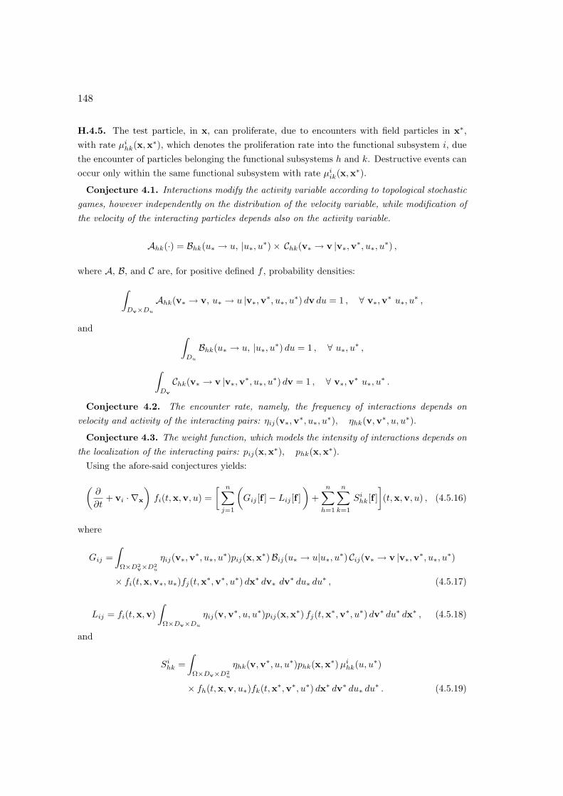
148
H.4.5. The test particle, in x, can proliferate, due to encounters with field particles in x∗,with rate µi
hk(x,x∗), which denotes the proliferation rate into the functional subsystem i, duethe encounter of particles belonging the functional subsystems h and k. Destructive events canoccur only within the same functional subsystem with rate µi
ik(x,x∗).
Conjecture 4.1. Interactions modify the activity variable according to topological stochasticgames, however independently on the distribution of the velocity variable, while modification ofthe velocity of the interacting particles depends also on the activity variable.
Ahk(·) = Bhk(u∗ → u, |u∗, u∗)× Chk(v∗ → v |v∗,v∗, u∗, u∗) ,
where A, B, and C are, for positive defined f , probability densities:
∫
Dv×Du
Ahk(v∗ → v, u∗ → u |v∗,v∗, u∗, u∗) dv du = 1 , ∀ v∗,v∗ u∗, u∗ ,
and ∫
Du
Bhk(u∗ → u, |u∗, u∗) du = 1 , ∀ u∗, u∗ ,
∫
Dv
Chk(v∗ → v |v∗,v∗, u∗, u∗) dv = 1 , ∀ v∗,v∗ u∗, u∗ .
Conjecture 4.2. The encounter rate, namely, the frequency of interactions depends onvelocity and activity of the interacting pairs: ηij(v∗,v∗, u∗, u∗), ηhk(v,v∗, u, u∗).
Conjecture 4.3. The weight function, which models the intensity of interactions depends onthe localization of the interacting pairs: pij(x,x∗), phk(x,x∗).
Using the afore-said conjectures yields:
(∂
∂t+ vi · ∇x
)fi(t,x,v, u) =
[ n∑
j=1
(Gij [f ]− Lij [f ]
)+
n∑
h=1
n∑
k=1
Sihk[f ]
](t,x,v, u) , (4.5.16)
where
Gij =∫
Ω×D2v×D2
u
ηij(v∗,v∗, u∗, u∗)pij(x,x∗)Bij(u∗ → u|u∗, u∗) Cij(v∗ → v |v∗,v∗, u∗, u∗)
× fi(t,x,v∗, u∗)fj(t,x∗,v∗, u∗) dx∗ dv∗ dv∗ du∗ du∗ , (4.5.17)
Lij = fi(t,x,v)∫
Ω×Dv×Du
ηij(v,v∗, u, u∗)pij(x,x∗) fj(t,x∗,v∗, u∗) dv∗ du∗ dx∗ , (4.5.18)
and
Sihk =
∫
Ω×Dv×D2u
ηhk(v,v∗, u, u∗)phk(x,x∗) µihk(u, u∗)
× fh(t,x,v, u∗)fk(t,x∗,v∗, u∗) dx∗ dv∗ du∗ du∗ . (4.5.19)
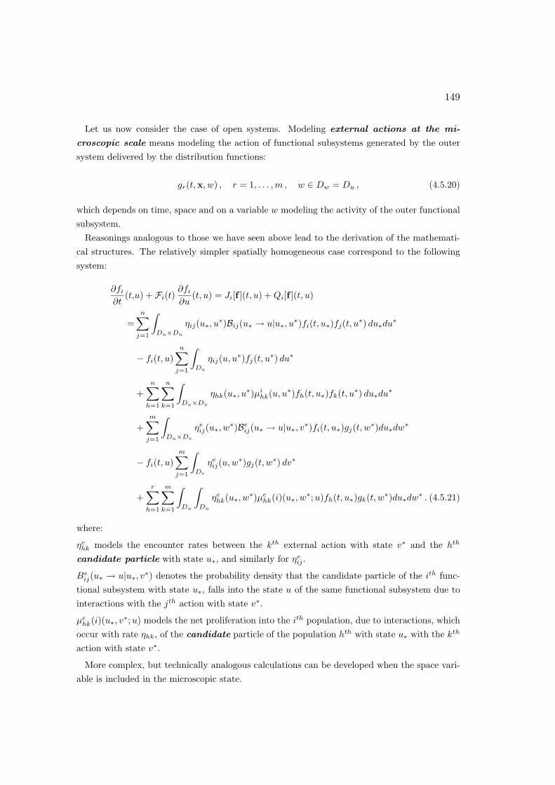
149
Let us now consider the case of open systems. Modeling external actions at the mi-
croscopic scale means modeling the action of functional subsystems generated by the outersystem delivered by the distribution functions:
gr(t,x, w) , r = 1, . . . , m , w ∈ Dw = Du , (4.5.20)
which depends on time, space and on a variable w modeling the activity of the outer functionalsubsystem.
Reasonings analogous to those we have seen above lead to the derivation of the mathemati-cal structures. The relatively simpler spatially homogeneous case correspond to the followingsystem:
∂fi
∂t(t,u) + Fi(t)
∂fi
∂u(t, u) = Ji[f ](t, u) + Qi[f ](t, u)
=n∑
j=1
∫
Du×Du
ηij(u∗, u∗)Bij(u∗ → u|u∗, u∗)fi(t, u∗)fj(t, u∗) du∗du∗
− fi(t, u)n∑
j=1
∫
Du
ηij(u, u∗)fj(t, u∗) du∗
+n∑
h=1
n∑
k=1
∫
Du×Du
ηhk(u∗, u∗)µihk(u, u∗)fh(t, u∗)fk(t, u∗) du∗du∗
+m∑
j=1
∫
Du×Dv
ηeij(u∗, w
∗)Beij(u∗ → u|u∗, v∗)fi(t, u∗)gj(t, w∗)du∗dw∗
− fi(t, u)m∑
j=1
∫
Dv
ηeij(u,w∗)gj(t, w∗) dv∗
+r∑
h=1
m∑
k=1
∫
Du
∫
Du
ηehk(u∗, w∗)µe
hk(i)(u∗, w∗; u)fh(t, u∗)gk(t, w∗)du∗dw∗ . (4.5.21)
where:
ηehk models the encounter rates between the kth external action with state v∗ and the hth
candidate particle with state u∗, and similarly for ηeij .
Beij(u∗ → u|u∗, v∗) denotes the probability density that the candidate particle of the ith func-
tional subsystem with state u∗, falls into the state u of the same functional subsystem due tointeractions with the jth action with state v∗.
µehk(i)(u∗, v∗;u) models the net proliferation into the ith population, due to interactions, which
occur with rate ηhk, of the candidate particle of the population hth with state u∗ with the kth
action with state v∗.
More complex, but technically analogous calculations can be developed when the space vari-able is included in the microscopic state.

150
4.6 Some Preliminary Ideas on the Modeling of Nonlinear Interactions
It is well understood that interactions involving living entities may be nonlinearly additive.A brief introduction is given in this subsection. Some sources of nonlinearity are the following:
• Encounter rate depending on the distribution function due to the hiding and learning
dynamics;
• Table of games conditioned by the distribution function;
• Nonlinearity induced by topological distribution of the interacting entities.
The modeling of the learning dynamics refers to the seminal paper by Cucker and Smale(2002). This paper presents a deep and exhaustive understanding of the approximation ofsparse data, viewed as learning, i.e. the information to be learned.
Here some preliminary ideas are proposed, referring to Bellomo (2010), on the modelingapproach to hiding and learning dynamics of two interacting functional subsystems, wherethe first one escapes, while the second one hunts. The mathematical structure, which is aparticular case of (4.5.21), can be used:
∂fi
∂t(t, u) =
2∑
j=1
∫
Du×Du
ηij(u∗, u∗)Bij(u∗ → u|u∗, u∗) fi(t, u∗) fj(t, u∗) du∗ du∗
− fi(t, u)2∑
j=1
∫
Du
ηij(u, u∗) [1− µij(u, u∗)] fj(t, u∗) du∗. (4.6.1)
where: ηij and µij(u, u∗) the encounter rate and the proliferation rate related to the candidateactive particle, with state u∗, of the hth functional subsystem and the field active particle,with state u∗, of the jth functional subsystem. Moreover, Bij is the probability density that acandidate particle, with state u∗, of the ith functional subsystem ends up into the state u ofthe test particle of the same functional subsystem after the interaction with the field particle,with state u∗, of the jth functional subsystem.
The mathematical structure can be specialized into a mathematical model when the inter-action terms ηij and Bij are properly modeled according to a dynamics of hiding and learningactions. Specifically, let us consider the encounter rate in the following general form
ηij = η0ij e−c β2
ij(t|f ,u∗,u∗), (4.6.2)
where c is a positive constant and β2ij(t|f) models the distance between the two interacting
particles. In details, the following cases can be considered:
I – βij is equal to zero: This assumption corresponds to simplest approach that consistsin assuming that the encounter rate is identified only by the interacting pairs, so that it is aconstant η0
ij for each pair of interacting functional subsystems.

151
II – βij is the distance between the microscopic states of the two interacting pairs:
This amounts to suppose that βij is given by the difference between the microscopic state ofthe interacting particles, and it can be related to the interaction rate as follows:
βij(u∗, u∗) =√
(u∗ − u∗)2, ηij = η0ij e−c (u∗−u∗)2 . (4.6.3)
III – βij is given by the distance between the shapes of the distribution of the
two interacting subsystems: This corresponds to suppose that it is given by the differencebetween the shapes of the interacting particles. More precisely distance βij between the ith andthe jth functional subsystem can be defined as follows:
β2ij(t|f) =
∫
Du
(fi − fj)2(t, u) du, (4.6.4)
hence
ηij = η0ij e−cβ2
ij(t|f) = η0ij e
−c∫
Du(fi−fj)
2(t,u) du. (4.6.5)
More in general, the distance βij can be given by the norm of the difference between fi andfj in the appropriate metric space.
The dynamics is given by the following equation:
∂fi
∂t(t, u) =
2∑
j=1
∫
Du×Du
η0ij e−c β2
ij(t|f) Bij(u∗ → u|u∗, u∗) fi(t, u∗) fj(t, u∗) du∗ du∗
− fi(t, u)2∑
j=1
∫
Du
η0ij e−c β2
ij(t|f) [1− µij(u, u∗)] fj(t, u∗) du∗. (4.6.6)
This structure can be generalized to include the generation of new functional subsys-
tems as follows:
∂fi
∂t(t, u) =
p∑
h=1
p∑
k=1
∫
Du×Du
η0hk e−c β2
hk(t|f) Bihk(u∗ → u|u∗, u∗) fh(t, u∗) fk(t, u∗) du∗ du∗
− fi(t, u)p∑
k=1
∫
Du
η0ik e−c β2
ik(t|f) fk(t, u∗) du∗
+p∑
h=1
p∑
k=1
∫
Du×Du
η0hk e−c β2
hk(t|f)µihk(u∗, u∗)fh(t, u∗) fk(t, u∗) du∗ du∗, (4.6.7)
where Bihk is the probability density that a candidate particle of the hth functional subsystem,
with state u∗ ends up into the state u of the ith functional subsystem after the interactionwith the field particle of the kth functional subsystem, with state u∗. Moreover, µi
hk is theproliferative/destructive rate in the ith f.s. of the test particle, due to the encounter betweenthe hth candidate particle, with state u∗, of the kth particle (field), with state u∗.

152
Example 4.6.1
Modeling Hiding Learning Dynamics
A simple approach of modeling the terms Bij , for two functional subsystems, can be obtainedby supposing that the output of the interaction is defined by the most probable value mij andthe variance σij . In general it can be assumed that encounters within the same functionalsubsystem do not modify the state of the interacting pair:
• The candidate particle with activity u∗ does not shows any modification of its state relatedwhen it encounters a field particle of the same subsystem: m11 = m22 = u∗.
• The candidate particle of the first subsystem, with activity u∗, shows a trend to increasethe distance when it encounters the candidate particle of the second subsystem:
m12 =u∗ − ε1 (u∗ − u∗), if u∗ > u∗
m12 =u∗ + ε1 (u∗ − u∗), if u∗ ≤ u∗
• The candidate particle, with activity u∗, of the second subsystem shows a trend to reducethe distance with respect to the state of the candidate particle of the first subsystem:
m21 =u∗ − ε2 (u∗ − u∗), if u∗ < u∗
m21 =u∗ + ε2 (u∗ − u∗), if u∗ ≥ u∗
Let us now consider the case of nonlinear interactions where the term Bij , depend on thedistribution function of the interaction particles, for instance by the moments of such distribu-tion. The evolution equation for functional subsystems undergoing conservative interactions isas follows:
∂fi
∂t(t, u) = Ji[f ](t, u) =
n∑
j=1
Jij [fi, fj ](t, u)
=n∑
j=1
∫
Du×Du
ηij(t|fi, fj)Bij(u∗ → u|u∗, u∗, Ep[fi], Ep[fj ]) fi(t, u∗) fj(t, u∗) du∗ du∗
− fi(t, u)n∑
j=1
∫
Du
ηij(t|fi, fj) fj(t, u∗) du∗, (4.6.8)
More precisely, the idea is that the candidate particle interacts with the field particles withinits space interaction domain and feels an action identified by the low order moments of the fieldactive particles. The action can be also related, whether consistent with the specific systemunder consideration, to their most probable value, see Bellomo et al. (2010b). This paper alsoshows that the interaction domain of the candidate particle with state u∗ may not be the whole

153
domain Du but a subset Ωu∗ ⊆ Du, which contains the field particles u∗ ∈ Ωu∗ that are ableto interact with candidate particle. Thus interactions only occur if the distance, in the spaceof microscopic states of the interacting particles, are sufficiently small. Therefore a positivefunction ω(u∗, u∗), normalized with respect to integration over u∗, is introduced to take intoaccount such dynamics. This function, which weight the interactions among the active particles,is assumed to have a compact support in the domain of influence Ωu∗ ⊆ Du of the interactions.Moreover: ∫
Du
ω(u∗, u∗) du∗ =∫
Ωu∗
ω(u∗, u∗) du∗ = 1. (4.6.9)
Accordingly we define the pth order weighted moment as follows:
Epw[fi](t, u∗) =
∫
Du
(u∗)p ω(u∗, u∗) fi(t, u∗) du∗ =∫
Ωu∗
(u∗)p ω(u∗, u∗) fi(t, u∗) du∗. (4.6.10)
The mathematical structure is as follow:
∂fi
∂t(t, u) = Qi[f ](t, u) =
n∑
h,k=1
Qhk[fh, fk](t, u)
=n∑
h=1
n∑
k=1
∫
Du×Du
η0hke−cβ2
hk(t|fh,fk)Bihk(u∗ → u|u∗, u∗, Ep
w[fh], Epw[fk])fh(t, u∗)fk(t, u∗)du∗du∗
− fi(t, u)n∑
k=1
∫
Du
η0ik e−c β2
ik(t|fi,fk) fk(t, u∗) du∗
−n∑
h=1
n∑
k=1
∫
Du×Du
η0hk e−c β2
hk(t|fh,fk)µihk(u∗, u∗)fh(t, u∗) fk(t, u∗) du∗ du∗. (4.6.11)
where the number of particles is not any more constant in time due to the term that modelsproliferative and/or destructive events. In details:
• µihk models the proliferative/destructive rate of particles of the hth functional subsystem,
with state u∗, into the state u of the ith functional subsystem due to the encounter with theparticle (field) of the kth functional subsystem, with state u∗. In particular, destructive eventsoccur only within the functional subsystem of the field particles.
• Bihk models the probability density that a candidate particle of the hth functional subsystem,
and with state u∗, ends up into the state u of the ith functional subsystem after the interactionwith the field particle, with state u∗, of the kth functional subsystem.
The application of the mathematical approach we have seen in the preceding and in thissections can be practically applied to model vehicular traffic dynamics, namely a class ofcomplex systems already treated various times in these Lectures Notes. Three aspects willbe considered, and treated in the forthcoming examples; namely, the derivation of the math-ematical structure suitable to capture the complexity of the system under consideration, the

154
derivation of the table of games modeling interactions at the microscopic scale and the val-idation by using empirical data. The book by Kerner (2004) offers a valuable collection ofexperimental results followed by a sharp interpretation based on the physics of traffic, whilethe review papers by Helbing (2001) and Bellomo and Dogbe (2011) provide the mathematicalbackground for the kinetic theory approach to modeling vehicular traffic phenomena.
Let us recall, repeating some concepts of the preceding chapters, that the modeling shouldbe developed by using dimensionless quantities. Referring specifically to the maximum densitynM of vehicles corresponding to bumper-to-bumper traffic jam, and to the maximum admissiblemean velocity VM which can be reached, in average, by vehicles running in free flow conditions,while a fast isolated vehicle can reach velocities larger that VM . More precisely, a limit velocitycan be defined as follows: V` = (1+µ)VM , with µ > 0, such that no vehicle can reach, simply bymechanical reasons, a velocity larger than V`. Moreover, it is convenient, to identify the criticaltime Tc as the ratio between ` and VM . Moreover, t is the dimensionless time variable obtainedreferring the real time tr to a suitable critical time Tc = `/VM , while x is the dimensionlessspace variable obtained dividing the real space xr by the length ` of the road.
The modeling approach can be based on a strategy defined by the following reasonings:
• Increasing the complexity of the model increases the number of parameters to be identified.
• The system is with finite degrees of freedom. However, microscopic models induce considerableerrors in the computation of macroscopic quantities.
• The flow is not continuous, hence hydrodynamic models should not be used. Moreover, it isdifficult to evaluate the entity of the approximation induced by macro-models.
• The number of individual entities is not large enough to allow the use of continuous distributionfunctions within the framework of the mathematical kinetic theory. Moreover, interactions arenot localized, considering that drivers adapt the dynamics of the vehicle to the flow conditionsin the visibility zone.
• Individual entities cannot be regarded as classical particles, but as active particles due to theirability to modify their dynamics according to specific strategies.
The examples proposed in the following tackle the afore-said specific modeling issues andrefer to the recent paper Bianca and Coscia (2011).
Example 4.6.2
Representation and Mathematical Structure of Vehicular Traffic
Let us consider discrete velocity models, where the velocity variable belongs to the followingset: Iv = v1 = 0 , . . . , vi , . . . , vn = 1. The corresponding discrete representation is obtainedby linking the discrete distribution functions to each vi: fi = fi(t, x) : IR+ × [0, 1] → IR+, fori = 1, . . . , n.
Macroscopic quantities are obtained by weighted sums. For instance, dimensionless number
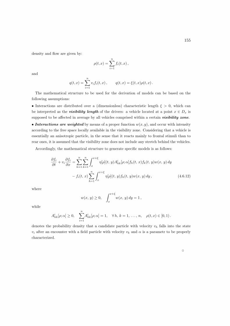
155
density and flow are given by:
ρ(t, x) =n∑
i=1
fi(t, x) ,
and
q(t, x) =n∑
i=1
vifi(t, x) , q(t, x) = ξ(t, x)ρ(t, x) .
The mathematical structure to be used for the derivation of models can be based on thefollowing assumptions:
• Interactions are distributed over a (dimensionless) characteristic length ξ > 0, which canbe interpreted as the visibility length of the drivers: a vehicle located at a point x ∈ Dx issupposed to be affected in average by all vehicles comprised within a certain visibility zone.
• Interactions are weighted by means of a proper function w(x, y), and occur with intensityaccording to the free space locally available in the visibility zone. Considering that a vehicle isessentially an anisotropic particle, in the sense that it reacts mainly to frontal stimuli than torear ones, it is assumed that the visibility zone does not include any stretch behind the vehicles.
Accordingly, the mathematical structure to generate specific models is as follows:
∂fi
∂t+ vi
∂fi
∂x=
n∑
h=1
n∑
k=1
∫ x+ξ
x
η[ρ](t, y)Aihk[ρ; α]fh(t, x)fk(t, y)w(x, y) dy
− fi(t, x)n∑
h=1
∫ x+ξ
x
η[ρ](t, y)fh(t, y)w(x, y) dy , (4.6.12)
where
w(x, y) ≥ 0,
∫ x+ξ
x
w(x, y) dy = 1 ,
while
Aihk[ρ;α] ≥ 0,
n∑
i=1
Aihk[ρ; α] = 1, ∀h, k = 1, . . . , n, ρ(t, x) ∈ [0, 1) .
denotes the probability density that a candidate particle with velocity vh falls into the statevi after an encounter with a field particle with velocity vk and α is a parametr to be properlycharacterized.

156
Example 4.6.3
Modeling Interactions of Vehicles
The modeling of interactions, according to Bianca and Coscia (2011) uses a parameter α ∈ [0, 1]is related to the quality of the road:
α =ρc
ρcM
, α ∈ [0, 1] ,
where ρcM is the maximal admissible value corresponding to the best highway in optimalenvironmental conditions.
The velocity is discretized by coupling of a steady grid when the density ρ is less than thecritical one ρc and with an adaptive grid when ρ is greater than ρc:
vi =2i− 1n− 1
if 0 ≤ ρ ≤ ρc,
vi =(1 + α) (1− ρ3)2i− 1n− 1
if ρc < ρ ≤ 1,
for i ∈ 1, . . . , nThe encounter rate nhk, for h, k ∈ 1, . . . , n, is assumed as follows: ηhk = |vh − vk|. The
Table of the Games Aihk can be derived according to the following assumptions:
i) The trend of the candidate particle to change its velocity decreases in probability when the“distance” |vh − vk| between the velocity of the candidate and field vehicle decreases.
ii) The candidate vehicle h can attain only a velocity vi ∈ vh, vh−1, . . . , vk if it interacts witha field vehicle with velocity vk such that vh > vk while if the candidate vehicle interacts witha field vehicle such that vh < vk it can only attain a velocity vi ∈ vh, vh+1, . . . , vk.
iii) If the candidate and field vehicles have the same velocity, the interaction does not imply achange in velocity.
iv) When a candidate vehicle, with velocity vh, encounters a field vehicle, with velocity vk > vh
(faster vehicle), the candidate vehicle has a trend to increase its velocity from vh to vk.
v) When a candidate vehicle, with velocity vh, encounters a field vehicle, with velocity vk < vh
(slower vehicle), the candidate vehicle has a trend to decrease its velocity from vh to vk.
Detailed calculations reported in the afore stated paper provide the following results:
k < h, i = h : Aihk = 1− εhk ,
k < h, k ≤ i < h : Aihk =
εhk
|h− k|,
k > h, h < i ≤ h : Aihk =
εhk
|h− k|,
k > h, i = h : Aihk = 1− εhk ,

157
where
εhk = α1− ρ
|h− k|2 ·
Let us finally consider the problem of the validation of models. Three types of empirical datacan be classified:
Quantitative data, which provide accurate data of macroscopic quantities such as numberdensity, mean velocity, and/or flow. Models are required to have the ability to reproduce themquantitatively.
Qualitative data on emerging behaviors, which corresponds to specific conditions, forinstance in vehicular traffic interactions of clusters of fast and slow vehicles, bottlenecks. Modelare required to reproduce qualitatively emerging behaviors.
Data on individual behaviors, which should be used to design models for the table ofgames.
A remarkable difficulty is that quantitative and qualitative empirical data provide macro-
scopic quantities, while the dynamics is ruled at the microscopic scale. Moreover:
• The averaging process which leads to macroscopic quantities introduces unavoidable fluctua-tions due not only to measurement errors, but also to the stochastic and granular essence of theflow, where deceleration and acceleration of vehicles are observed even in almost steady flowstop and go dynamics;
• Generally, experimental results refer to steady state conditions, while rarely traffic
reach a steady state;
• Empirical data show results very sensitive to the quality of environmental conditions.Therefore, it is impossible to identify a unique deterministic representation.
• Kerner (2004) remarks that additional transitions can be observed when the flow is congested,for instance related to a considerable dispersion of data. Moreover, transitions have to beinterpreted carefully due to their variability with environmental conditions.
• The use of quantitative data as a direct input to derive models is an abuse as, at leastin principles, a careful modeling of microscopic interactions should provide the above result.
The interested reader can obtain a deeper understanding of the topic treated in this sectionby Bianca and Coscia (2010), where it is shown that their model remarkably reproduce allquantitative features of the velocity diagram studied by Kerner (2004). This diagram reportsthe mean velocity versus density and shows that there exists a critical density ρc such that forρ < ρc the mean velocity maintains its maximum value, while for ρ > ρc a sharp decay indicatesthe transition from free to congested flow. This characteristic, and specifically ρc, depends onthe quality of the outer environment. Additional information is obtained by Delitala and Tosin(2007), where it is shown that various emerging behaviors are reproduced by their model.

158
4.7 Critical Analysis
A concise introduction to some models of the kinetic theory for classical and active particleshas been given in this chapter, while suitable bibliographical indications have been providedtoward a deeper knowledge on the topics treated in this chapter have been given.
The substantial difference between models for classical and active particles refers to mi-croscopic interactions. Classical particles follow deterministic laws of Newtonian mechanics,namely if both the input velocities and the impact parameter are assigned, then the outputvelocities can be computed. On the other hand, interactions for active particles are stochastic.Moreover the activity variable can modify the mechanical variables due to the strategy of theparticles to modify their dynamics.
Although this chapter does not report specific applications, some bibliographical indicationscan be given. Specifically, the Boltzmann equation has been applied to study a variety of fluiddynamic problems at large Knudsen number. Various applications are documented in the booksby Kogan (1969). The Vlasov equation has been applied to study various problems in plasmaphysics, see for example Schram (1991).
The Kinetic Theory of Active Particles has been used to model some interesting complexsystems in applied sciences which are constituted by a large number of interacting entitiessuch that their microscopic state includes, in addition to geometrical and mechanical variable,an additional microscopic state related to their behavior, which will be called characteristic
microscopic variable, or simply: activity. Microscopic interactions do not follow rules ofmechanics (classical or quantum), but are governed by a somehow organized behavior which isable to modify laws of mechanics.
As already mentioned in Chapter 1, mathematical models of the kinetic theory are used toovercame complexity problems induced by the need of modeling large systems of interacting in-dividuals, where the number of equations needed to describe the system is not computationallytractable. The representation offered by methods of the mathematical kinetic theory is elegantand efficient. On the other hand the derivation of equations is based on heuristic assumptions(for instance the factorization of the joint probability density), that cannot be rigorously jus-tified. Therefore, models of the kinetic theory have to be regarded as an approximation of thephysical reality considering that even the structures, that the models refer to, are based onmathematical approximations. Of course, various approaches to improve the above mentionedapproximations have been developed. However, we do not discuss this difficult topic in theseLecture Notes.
Technically, different are the complexity problems related to models of active particles. Infact, velocities of elements of living systems are always bounded, as documented in all appli-cations dealt with in the book Bellomo (2008). Therefore, complexity problems are related tomodeling microscopic interactions rather than to the development of computational algorithms.Discretization can be viewed as an approach to capture the main feature of the activity variablein view of modeling microscopic interactions.

159
Finally, let us stress again that the various reasonings proposed in this chapter have to beregarded simply as a brief introduction to modeling systems in applied and life sciences by theapproach of the classical and generalized kinetic theory. This brief introduction has the objectiveto motivate the reader to a deeper insight, that may possibly start from the bibliography citedin this chapter.

160

161
Chapter 5
Bibliography
Arlotti L., Bellomo N., De Angelis E., and Lachowicz M., (2003), General-
ized Kinetic Models in Applied Sciences - Lecture Notes on Mathematical
Problems, World Scientific, London, Singapore.
Arlotti L., Bellomo N., Lachowicz M., Polewczak J., and Walus W., (1995),
Lecture Notes on the Mathematical Theory of the Boltzmann Equation, World
Scientific, London, Singapore.
Bellomo N., (1998), Guest Editorial: Perspectives on the relationship between math-
ematics and engineering sciences, Appl. Mech. Reviews, 51, iii)–iv).
Bellomo N., (2008), Modelling Complex Living Systems - A Kinetic Theory
and Stochastic Game Approach, Birkhauser, Boston.
Bellomo N., Berestycki H., Brezzi F., and Nadal J.P., (2010a), Mathematics
and Complexity in Life and Human Sciences, Math. Models Methods Appl. Sci, 20,
1391–1396.
Bellomo N., Bianca C., and Delitala M., (2009), Complexity analysis and mathe-
matical tools towards the modeling of living systems, Physics of Life Reviews, 6, 144–175.
Bellomo N., Bianca C., and Mongiovi M.S., (2010b), On the modeling of nonlin-
ear interactions in large complex systems, Appl. Math. Lett., 23, 1372–1377.
Bellomo N., and Carbonaro B., (2011), Toward a mathematical theory of living
systems focusing on developmental biology and evolution: A review and perspectives,
Physics of Life Reviews, to appear.
Bellomo N., Coscia V., and Delitala M., (2002), On the mathematical theory of
vehicular traffic flow. I. Fluid dynamic and kinetic modelling, Math. Models Methods

162
Appl. Sci., 12, 1801–1843.
Bellomo N. and Dogbe C., (2011), On the modeling of traffic and crowds a survey
of models, speculations, and perspectives, SIAM Rev., to appear.
Bellomo N. and Gustafsson T., (1991), The discrete Boltzmann equation: a review
of the mathematical aspects of the initial and initial-boundary value problems, Rev.
Math. Phys., 3, 137–162.
Bellomo N., Lods B., Revelli R., and Ridolfi L., (2007), Generalized Colloca-
tion Methods - Solutions to Nonlinear Problems, Birkhauser, Boston.
Bellomo N. and Preziosi L., (1995), Modelling Mathematical Methods and
Scientific Computation, CRC Press, Boca Raton.
Bellomo N., Preziosi L., and Romano A., (2000), Mechanics and Dynamic
Systems with Mathematica, Birkhauser, Boston.
Bellouquid A. and Delitala M., (2006), Mathematical Modeling of Complex
Biological Systems. A Kinetic Theory Approach, Birkhauser, Boston.
Bertotti M.L. and Delitala M., (2004), From discrete kinetic and stochastic game
theory to modelling complex systems in applied sciences, Math. Models Methods Appl.
Sci., 14, 1061–1084.
Cercignani C., Illner R., and Pulvirenti M., (1994), The Mathematical The-
ory of Dilute Gases, Springer-Verlag, New York.
Cucker F. and Smale S., (2002), On the mathematical foundations of learning, Bull.
Amer. Math. Soc., 39, 1–49.
Dautray R. and Lions J.L., (1990), Mathematical Analysis and Numerical
Methods for Science and Technology - Vol. I, Springer-Verlag, Berlin.
De Angelis E., (1999), Nonlinear hydrodinamic models of traffic flow modelling and
mathematical problems, Math. Comput. Modelling, 29, 83–95.
De Jager E.M. and Furu J., (1996), The Theory of Singular Perturbations,
North-Holland, Amsterdam.
Gatignol R., (1975), Theorie Cinetique des Gaz a Repartition Discrete de
Vitesses, Springer-Verlag, Berlin-New York.
Glassey R., (1996), The Cauchy Problem in Kinetic Theory, SIAM Publish.,
Philadelphia.
Gorsch D., (2002), Generalized discrete velocity models, Math. Models Methods Appl.
Sci., 12, 49–75.
Helbing D., (2001), Traffic and related self-driven many-particle systems, Rev. Modern
Phys., 73, 1067–1141.

163
Humi M. and Miller W., (1988), Second Course in Ordinary Differential Equa-
tions for Scientists and Engineers, Springer-Verlag, New York.
Jager E. and Segel L., (1992), On the distribution of dominance in populations of
social organisms. SIAM J. Appl. Math., 52, 1442–1462.
Kerner B., (2004), The Physics of Traffic, Springer, New York, Berlin.
Klar A., Kuhne R.D., and Wegener R., (1996), Mathematical models for vehicular
traffic, Surveys Math. Indust., 6, 215–239.
Kogan M.N., (1969), Rarefied Gas Dynamics, Plenum Press, New York.
Kojic M. and Bathe K.J., (2005), Inelastic Analysis of Solids and Structures,
Springer-Verlag, Berlin.
Lions J.L. and Magenes E., (1968), Problemes aux Limites Non Homogenes
et Application - Vol. I, Dunod, Paris.
May R.M., (2004), Uses and abuses of mathematics in biology. Science, 303, 790–793.
Marasco A. and Romano A., (2001), Scientific Computing with Mathemati-
ca c©. Mathematical Problems for Ordinary Differential Equation, Birkhauser,
Boston.
Mika, J.R. and Palczewski A., (1991), Asymptotic analysis of singularly perturbed
systems of ordinary differential equations, Comput. Math. Appl., 21, 13–32.
Mishchenko E.F. and Rozov N.Kh., (1980), Differential Equations with Small
Parameters and Relaxation Oscillations, Plenum Press, New York.
O’Malley R.O., (1991), Singular Perturbation Methods for Ordinary Differ-
ential Equations, Springer-Verlag, New York.
Platkowski T. and Illner R., (1988), Discrete velocity models of the Boltzmann
equation: a survey on the mathematical aspects of the theory, SIAM Rev., 30, 213–255.
Pontriaguine L., (1975), Equations Differentielles Ordinaries, Editions MIR,
Moscow.
Prigogine I. and Herman R., (1971), Kinetic Theory of Vehicular Traffic,
Elsevier, New York.
Reed R., (2004), Why is mathematical biology so hard? Notices of the American
Mathematical Society, 51, 338–342.
Schram P.P.J.M., (1991), Kinetic Theory of Gases and Plasmas, Kluwer Aca-
demic Publishers Group, Dordrecht.
Truesdell C. and Rajagopal K., (2000), An Introduction to the Mechanics of
Fluids, Birkhauser, Boston.

164