appendix 7 technical analysis - caltrans · appendix 7 . technical analysis . 2-29-16 ctp 2040...

2-29-16 CTP 2040 Final Review Draft

Appendix 7

Technical Analysis


APPENDIX 7 | TECHNICAL ANALYSIS

INTRODUCTION This report describes the technical analyses conducted to evaluate theoretical greenhouse gas (GHG) reduction strategies and economic benefits contained in the California Transportation Plan 2040 (CTP 2040) scenarios that are designed to test one possible scenario to reach the state’s GHG reduction targets. Key technical analyses were conducted using the California Statewide Travel Demand Model (CSTDM), the California Air Resources Board’s (ARB’s) EMissions FACtor (EMFAC) and ARB’s Vision for Clean Air (VISION) Models, and the Transportation Economic Development Impact Software (TREDIS).

Draft analysis results, completed in early 2015, were subsequently updated for the final forecasts contained in this report. Key changes between the draft and final CTP 2040 include the following:

• Modeled expanded pricing policies with a statewide auto operating cost increase of 36.5 percent (equivalent to 16 cents a miles) and an additional increase of 36.5 percent in urban areas (expressed in increases to auto operating costs) designed to simulate a theoretical urban county congestion fee.

• Roll back modeled transit vehicle speed increases to 50 percent above Scenario 1 (draft CTP 2040 included a doubling of transit vehicle speeds).

• San Joaquin Valley vehicle miles traveled (VMT) adjusted down by 11.6 percent in the modeling strategy, from the DRAFT model runs, to account for slower expected growth in population and jobs.

• Increased high occupancy vehicle (HOV) lane strategy, analyzed off-model, and assumed to decrease statewide VMT by 1.0 percent for this exercise.

CALIFORNIA STATEWIDE TRAVEL DEMAND MODEL The CSTDM was recently updated using the most current information from the 2012 CHTS, the 2010 US Census, and assumptions from California Metropolitan Planning Organization (MPO) Sustainable Communities Strategies (SCSs), effective Spring 2013. The CSTDM (dubbed CSTDM Version 2.0) is documented at the California Department of Transportation (Caltrans) website at http://www.dot.ca.gov/hq/tpp/offices/omsp/statewide_modeling/cstdm.html.

The CSTDM is an integrated system of five components of typical weekday travel in California:

• Short distance personal travel • Long distance personal travel • Short distance truck travel • Long distance truck travel • Interregional Travel (from other states and Mexico)

The CSTDM also includes all modes of transportation, including bicycling, walking, flying, taking transit, trucks, and all passenger rail, including high-speed rail (HSR) (HSR included only for future year


forecasts). A summary of model components and modes of travel is shown in Table 1. Modes of travel are restricted to those logically associated with each model. For example, the long and short distance personal travel models do not allow for commercial truck travel. The long distance personal travel model excludes walk and bicycle trips, and HSR is excluded from short distance personal travel.

TABLE 1. CSTDM MODES OF TRAVEL FOR EACH MODEL COMPONENT

Models

Travel Modes Short

Distance Personal

Long Distance Personal

Short Distance

Truck

Long Distance

Truck

External Travel

Auto Single Occupant √ √ √

Auto 2 persons √ √ √

Auto 3+ persons √ √ √

Transit (bus and urban rail)

√

Bicycle √

Walk √

Air √

Intercity Rail / HSR √

Trucks (3 classes x weight)

√ √ √

VMT and Mobility Results

A key metric for CTP 2040 was VMT, which was used in the development of transportation GHG reduction strategies, as described in Chapter 3. Statewide daily VMT has been summarized for each horizon year (2010, 2020, and 2040) and by scenario. VMT rises through 2040 as the State’s population and economy increase. Substantial reductions in VMT are shown for Scenarios 2 and 3 compared to Scenario 1. VMT was used as a metric to be consistent among the strategies, as well as provide for comparison of the strategies. However, GHG reduction is the ultimate goal of the scenarios and


strategies and not specifically VMT reduction. VMT is used as a surrogate in the models for reductions in GHG remissions.

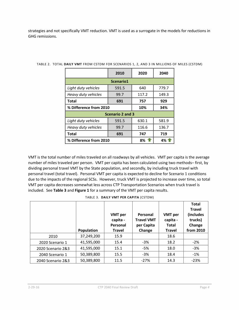
TABLE 2. TOTAL DAILY VMT FROM CSTDM FOR SCENARIOS 1, 2, AND 3 IN MILLIONS OF MILES (CSTDM)

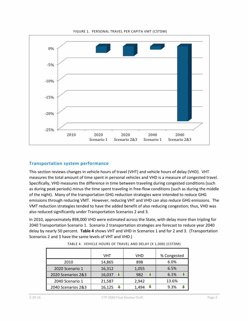
VMT is the total number of miles traveled on all roadways by all vehicles. VMT per capita is the average number of miles traveled per person. VMT per capita has been calculated using two methods– first, by dividing personal travel VMT by the State population, and secondly, by including truck travel with personal travel (total travel). Personal VMT per capita is expected to decline for Scenario 1 conditions due to the impacts of the regional SCSs. However, truck VMT is projected to increase over time, so total VMT per capita decreases somewhat less across CTP Transportation Scenarios when truck travel is included. See Table 3 and Figure 1 for a summary of the VMT per capita results.

TABLE 3. DAILY VMT PER CAPITA (CSTDM)

Population

VMT per capita -

Personal Travel

Personal Travel VMT per Capita

Change

VMT per capita -

Total Travel

Total Travel

(includes trucks) Change

from 2010 2010 37,249,200 15.9 18.6

2020 Scenario 1 41,595,000 15.4 -3% 18.2 -2% 2020 Scenario 2&3 41,595,000 15.1 -5% 18.0 -3%

2040 Scenario 1 50,389,800 15.5 -3% 18.4 -1% 2040 Scenario 2&3 50,389,800 11.5 -27% 14.3 -23%

2010 2020 2040

Scenario1 Light duty vehicles 591.5 640 779.7 Heavy duty vehicles 99.7 117.2 149.3 Total 691 757 929 % Difference from 2010 10% 34%

Scenario 2 and 3 Light duty vehicles 591.5 630.1 581.9 Heavy duty vehicles 99.7 116.6 136.7 Total 691 747 719 % Difference from 2010 8% 4%


Transportation system performance

This section reviews changes in vehicle hours of travel (VHT) and vehicle hours of delay (VHD). VHT measures the total amount of time spent in personal vehicles and VHD is a measure of congested travel. Specifically, VHD measures the difference in time between traveling during congested conditions (such as during peak periods) minus the time spent traveling in free-flow conditions (such as during the middle of the night). Many of the transportation GHG reduction strategies were intended to reduce GHG emissions through reducing VMT. However, reducing VHT and VHD can also reduce GHG emissions. The VMT reduction strategies tended to have the added benefit of also reducing congestion; thus, VHD was also reduced significantly under Transportation Scenarios 2 and 3.

In 2010, approximately 898,000 VHD were estimated across the State, with delay more than tripling for 2040 Transportation Scenario 1. Scenario 2 transportation strategies are forecast to reduce year 2040 delay by nearly 50 percent. Table 4 shows VHT and VHD in Scenarios 1 and for 2 and 3. (Transportation Scenarios 2 and 3 have the same levels of VHT and VHD.)

TABLE 4. VEHICLE HOURS OF TRAVEL AND DELAY (X 1,000) (CSTDM)

VHT VHD % Congested

2010 14,865 898 6.0% 2020 Scenario 1 16,312 1,055 6.5%

2020 Scenarios 2&3 16,037 982 6.1% 2040 Scenario 1 21,587 2,942 13.6%

2040 Scenarios 2&3 16,125 1,494 9.3%

-25%

-20%

-15%

-10%

-5%

0%

2010 2020Scenario 1

2020Scenario 2&3

2040Scenario 1

2040Scenario 2&3

FIGURE 1. PERSONAL TRAVEL PER CAPITA VMT (CSTDM)


THEORETICAL TRANSPORTATION SCENARIOS

MPO/SCS Assumptions Used In Scenarios

As described in Chapter 3, the most up-to-date SCS and Regional Transportation Plan (RTP) assumptions were used for CTP 2040 analyses. However, SCS and RTP data developed after the Spring of 2013 were not included–most notably the eight San Joaquin Valley MPOs. The San Joaquin Valley MPOs have subsequently forecasted significantly lower demographic growth (population and jobs) for their 2014 SCSs, compared to prior regional plans. For the purposes of this report, an off-model VMT reduction was assumed for the San Joaquin Valley MPOs to better represent the more current lower estimates for population and employment growth. Those off-model adjustments are discussed further below in this Appendix.

As of Spring 2013, not all MPOs had completed RTPs that conformed to SB 375 requirements. Socio-economic forecasts and transportation improvement assumptions were included for the following MPOs:

• Bay Area Metropolitan Transportation Commission (MTC)

• Southern California Association of Governments (SCAG)

• Sacramento Area Council of Governments (SACOG)

• Santa Barbara County Association of Governments (SBCAG)

• San Luis Obispo Council of Governments (SLOCOG)

• Tahoe Regional Planning Agency (TRPA)

Additionally, socio-economic forecasts and transportation network assumptions that were updated, but not officially included in the final adopted RTP/SCS were also included for the following regions:

• Association of Monterey Bay Area Governments (AMBAG)

• Butte Council of Governments (BCAG)

County-level population forecast data were also updated for these counties:

• Del Norte County

• Humboldt County

Clean Fuel Assumptions Used in the Transportation Scenarios

In January 2012, the ARB approved a new emissions-control program for model years 2017 through 2025. The program combined the control of smog, soot, and global warming gases, and requirements for greater numbers of zero-emission vehicles (ZEVs) into a single package of standards called Advanced Clean Cars.

TRANSPORTATION GHG REDUCTION STRATEGIES Transportation GHG reduction strategies were outlined in Chapter 3. Appendix 7 presents a more thorough review of each strategy, including key GHG reduction assumptions. The contribution to GHG reductions is analyzed in terms of reduced VMT so each strategy can be compared on a one to one basis.


Table 5 summarizes the transportation GHG reduction strategies for each of the four categories–demand management, mode shift, travel cost, and operational efficiency.

TABLE 5. TRANSPORTATION GHG REDUCTION STRATEGIES BY CATEGORY

Demand Management Mode Shift Travel Cost Operational Efficiency

Telecommute/ Work at Home

Transit Service Improvements (Urban and intercity–rail, bus and ferry)

Implement Expanded Pricing Policies

Incident/Emergency Management

Increased carpoolers High-Speed Rail Caltrans' (TMS) Master Plan

Increased Car Sharing Bus Rapid Transit ITS/TSM

Expand Bike Eco-driving

Expand Pedestrian

Carpool Lane Occupancy Requirements

Increased HOV Lanes

Category 1: Demand Management

TELECOMMUTING STRATEGY

Telecommuting is the practice of working from home by employees who would otherwise travel to a workplace. Telecommuting usually requires the ability to communicate with coworkers electronically, by telephone, email, text message, and/or videoconference. Alternatively, telecommuters may work from a “telecommuting center,” also called a “telecenter,” that provides desk space, Internet access, and other basic support services but is located closer to home than the established workplace.1 The CTP 2040 assumes a statewide implementation of the telecommuting strategy.

The impact of increased telecommuting as an alternative to commuting was analyzed by SACOG as part of their Metropolitan Transportation Plan (MTP).2 SACOG forecasted a 0.39 percent VMT reduction as a result of more people working from home. The CTP 2040 used the same assumption on a statewide basis. See Table 6.

- - - - - - - - - - - - - - - - - - - - - - - - - - - - - 1 http://www.arb.ca.gov/cc/sb375/policies/telecommuting/telecommuting_brief.pdf 2 Sacramento Association of Governments, “2012 Metropolitan Transportation Plan, Final Environmental Impact Report,”

Appendix C-4, Model Reference Report, Sacramento, CA.

http://www.arb.ca.gov/cc/sb375/policies/telecommuting/telecommuting_brief.pdf


TABLE 6. VMT REDUCTIONS ASSOCIATED WITH INCREASED TELECOMMUTING

% Change Work at Home +2.1% Daily VMT reduced per worker 7.0 Change in VMT -0.39%

Source: SACOG; Assumes a 1:1 relationship between GHG reductions and VMT reductions.

CARPOOLING STRATEGY

The CTP 2040 assumes a 5 percent increase in the rate of carpooling statewide. Using data from the CSTDM, this carpooling strategy was estimated to reduce VMT by 2.9 percent statewide.

CARSHARING STRATEGY

Carsharing allows people to rent cars for a period of time extending from as little as 30 minutes, up to a full week. Carsharing services have been available in urbanized areas for over a decade, and in that time the number of subscribers and available vehicles has grown.3 The CTP 2040 assumes an aggressive implementation to increase the use of carsharing.

At the individual household level, carsharing could increase or decrease VMT. Carsharing may increase VMT for households that do not own automobiles, but other households with cars may choose to forego auto ownership (or own fewer vehicles) in favor of carsharing. An ARB Policy Brief examined two studies that found, "[R]eductions in VMT among vehicle-owners (or previous owners) who joined carsharing outweighed increases in VMT among non-owners who had joined at the time of the study. As a result, carsharing appears to have reduced VMT overall by about a quarter to a third among those who have participated.”4

MTC analyzed carsharing as part of their 2012 RTP.5 MTC assumed carsharing would increase region-wide due to new policies, such as the introduction of peer-to-peer carshare exchanges (which allows an individual to rent out his/her private vehicle when not in use), and one-way carsharing (in which vehicles are picked up in one location and returned to another). MTC assumed a net five percent increase in carsharing region-wide, with higher rates of penetration assumed in urbanized areas where carsharing already exists than in suburban areas where carsharing is beginning to be introduced. For the CTP 2040, a 5 percent increase in carsharing was assumed, and this resulted in a statewide reduction in VMT of 1.1 percent. See Table 7.

- - - - - - - - - - - - - - - - - - - - - - - - - - - - - 3 http://www.mtc.ca.gov/planning/plan_bay_area/draftplanbayarea/ 4 2013, Lovejoy, Handy and Boarnet, DRAFT Policy Brief on the Impacts of Carsharing (and Other Shared-Use Systems) Based on

a Review of the Empirical Literature, Prepared for California Air Resources Board, Sacramento, CA. 5 2013, Metropolitan Transportation Commission and Association of Bay Area Governments, Plan Bay Area Technical

Supplementary Report: Predicted Traveler Responses, Summary of Predicted Traveler Responses, Oakland, CA.

http://www.mtc.ca.gov/planning/plan_bay_area/draftplanbayarea/


TABLE 7. INCREASED CARSHARING ASSUMPTIONS, PLAN BAY AREA

EIR ALTERNATIVE URBAN AREAS SUBURBAN AREAS ALL AREAS

No Project (2020 and 2035) 10% 0% Car Share Alternatives (2035) 15% 5% Net change in Car Share Adoption Rates 5% 5% 5%

Source: Metropolitan Transportation Commission and Association of Bay Area Governments

Category 2: Mode Shift

TRANSIT SERVICE IMPROVEMENTS STRATEGY

Many different transit service-related improvements can be used to increase transit ridership. Transit services includes regularly scheduled urban, rural, and intercity transit services; this includes intercity, commuter, urban and light rail, bus services, and other transit line haul modes, such as cable cars and ferries.

For CTP 2040, an aggressive set of transit improvements was assumed. Transit service levels were assumed to double over 2040 baseline conditions, transit speeds for all services were assumed to increase by 50 percent, transit fares for all services were assumed to be free, and widespread timed transfers were also included.

The draft transit strategy has garnered a lot of attention as potentially unrealistic and unaffordable. As such, the final version of this analysis rolled back transit speed improvements from 100 percent faster to 50 percent faster. The intention to identify the maximum VMT reductions from transportation strategies has not shifted; however, doubling the speeds of all transit services in California was determined to not be practical for the purposes of this analysis.

The transit strategy was also designed to help offset road pricing by making transit a more viable option. Along with other alternative transportation strategies, dual emphases of reducing GHG emissions and increasing mobility options were paramount considerations.

Combined with the next strategy–reduced fares for HSR–the transit improvement strategy reduced statewide VMT by 6.0 percent.

HIGH-SPEED RAIL STRATEGY

The HSR system in the CTP 2040 is the same as assumed in the 2013 California State Rail Plan (CSRP) with service operating between the Los Angeles Region, San Joaquin Valley, and San Francisco Bay Area. HSR service levels and speeds are not changed from Transportation Scenario 1, but HSR fares are assumed to be reduced by 50 percent by 2040 in the modeling analysis to maximize incentives for ridership.


BUS RAPID TRANSIT STRATEGY

This strategy assumes that 20 percent of local bus services are converted to bus rapid transit (BRT). Traffic Congestion Relief Program (TCRP) Report 118: Bus Rapid Transit Practitioner’s Guide6 reviewed BRT improvements to local bus systems. Specific sets of improvements were not considered; rather, a combination of BRT improvements was assumed to meet the assumption of this strategy. Such improvements can include exclusive rights-of-way, limited-stop service, fare prepayment, signal priority, “branding” of the system, and other elements that enhance customer satisfaction.

The BRT strategy assumed that 20 percent of the local bus routes (or routes containing 20 percent of local bus riders) were converted from local bus to BRT. Using a series of assumptions, a modest VMT reduction of 0.07 percent was calculated as a result of the BRT strategy.

EXPANSION OF BICYCLE USE STRATEGY

The CTP 2040 assumes an aggressive implementation of the expansion of bicycle use, where the bicycle mode share is assumed to have doubled. Within the model, this objective projected a VMT decrease statewide of 0.4 percent. Some questions were raised whether the bicycle mode share could reasonably be expected to more than double over the 2040 Transportation Scenario 1 forecasts. However, absent compelling data, the doubling of the bicycle mode share was determined to be appropriate for Transportation Scenarios 2 and 3.

EXPANSION OF PEDESTRIAN ACTIVITIES STRATEGY

The CTP 2040 assumes an aggressive expansion of walking–a doubling of pedestrian mode shares. This objective assumed a VMT decrease statewide of 0.4 percent. As with the bicycle strategy, suggestions to increase the walk mode share beyond the initial assumption were made. The doubling of the walk mode share was also determined to be appropriate for Transportation Scenarios 2 and 3.

- - - - - - - - - - - - - - - - - - - - - - - - - - - - - 6 2007, Transit Cooperative Research Program, TCRP Report 118: Bus Rapid Transit Practitioner’s Guide, Washington DC.


CARPOOL LANE OCCUPANCY REQUIREMENTS STRATEGY

The required minimum carpool lane occupancies were increased from 2+ persons to 3+ persons for all carpool lanes statewide. Carpool lanes with 3+ occupancy rates were not modified; thus, a uniform 3+ carpool occupancy was assessed. This strategy was evaluated using the CSTDM and yielded a modest reduction of VMT by 0.8 percent statewide.

HOV LANE SYSTEM

The HOV or carpool lane system serves to increase the person-carrying capacities of California highways in many of the State’s largest regions. The HOT or express lanes provide preferential access for HOV or toll payment for facilities with excess peak period capacity.7 The CTP 2040 Transportation Scenario 1 includes the HOV/HOT network assumed in MPO SCSs, plus all of the widened and new roads contained in the MPO RTPs/SCSs.

The CTP Transportation Scenario 2 GHG reduction strategy extended the separate regional HOV systems into a seamless statewide inter-urban HOV network. The initial assumption was a series of additional new HOV lanes would be added throughout the State to connect the HOV network–particularly for interregional HOV access.

Transportation Scenario 2 did not assume any new lanes would be added to complete the HOV network–but rather that mixed flow lanes would be converted to HOV. The completed HOV network was not modeled directly using the CSTDM due to time constraints for producing the final CTP forecasts; rather, the completed HOV network was treated as an aspirational strategy, and assumed to reduce statewide VMT by 1.0 percent.

Category 3: Travel Cost

IMPLEMENT EXPANDED PRICING POLICIES

The utilization of pricing and vehicle fees to fund infrastructure improvements, manage congestion and improve roadways was modeled as a increase in auto operating cost throughout the State, plus an additional modeled increase designed to test a generalized congestion charge assessed in urban counties. Urban counties were defined as all county MPOs, except for Butte and Shasta Counties. Butte and Shasta were excluded from the generalized congestion charge because these MPOs are mostly surrounded by rural counties.

Non-MPO counties (plus Shasta and Butte) were all considered rural for this analysis. This strategy was designed to create a large mode shift in the model from single occupancy vehicle (SOV) trips to other alternative modes of transportation.

The Implement Expanded Pricing Policies strategy increased, in the model, 2040 statewide auto operating costs by 16 cents per mile. The urban congestion charge also increased auto operating costs by an additional 16 cents per mile. This totals the urban county increase in auto operating costs by 32 cents per mile. Table 8 shows the base auto operating cost assumptions used for 2010, 2020, and 2040.

- - - - - - - - - - - - - - - - - - - - - - - - - - - - - 7http://www.dot.ca.gov/hq/traffops/systemops/hov/Express_Lane/files/Caltrans%20HOV-ExpressLaneBizPlan%202009.pdf

http://www.dot.ca.gov/hq/traffops/systemops/hov/Express_Lane/files/Caltrans%20HOV-ExpressLaneBizPlan%202009.pdf


TABLE 8. AUTO OPERATING COST ASSUMPTIONS

Motor Gasoline in California -- Fuel Efficiency (mpg) -- Gas Operating Cost ($/mile) -- Non Gasoline Operating Cost ($/mile) -- 2010 Auto Operating Cost ($/mile) $0.23 Motor Gasoline in California $3.72 Fuel Efficiency (mpg) 24.1 Gas Operating Cost ($/mile) $0.15 Non Gasoline Operating Cost ($/mile) $0.09 2020 Auto Operating Cost ($/mile) $0.24 Motor Gasoline in California $4.83 Fuel Efficiency (mpg) 36.1 Gas Operating Cost ($/mile) $0.13 Non Gasoline Operating Cost ($/mile) $0.09 2040 Auto Operating Cost ($/mile) $0.22

Note: All figures in constant $2010.

Auto operating cost calculations are based on calculations made for travel demand modeling purposes only. The travel demand models do not consider the “sunk costs” of driving, such as car payments and insurance. As such, Table 9 below compares how CSTDM auto operating costs are calculated compared with real-life auto operating costs as calculated by the American Automobile Association (AAA).

TABLE 9. FACTORS IN AUTO OPERATING COST CALCULATIONS - AAA VERSUS CSTDM

Included: AAA CSTDM

Fuel √ √

Maintenance √ √

Tires √

Insurance √

License, Registration and Taxes √

Depreciation √

Finance √

Auto Operating Cost 59 cents/mile 22-24 cents / mile


Category 4: Operational Efficiency

INCIDENT AND EMERGENCY MANAGEMENT STRATEGY

Incident management programs identify, analyze, and correct minor and major traffic incidents to help mitigate traffic backups, as well as increase public safety. Incident management programs generally include three primary functions: 1) traffic surveillance–detecting and verifying traffic incidents, 2) clearance–coordinating emergency response teams to the site of the incident, and 3) traveler information–notifying motorists of the incident through changeable message signs to provide time to select a route that avoids the incident.8 Incident and emergency management is one component of Caltrans’ Transportation System Management and Operation (TSMO) program. The CTP 2040 assumes the implementation of all components of TSMO.

CALTRANS’ TRANSPORTATION MANAGEMENT SYSTEM MASTER PLAN STRATEGY

Caltrans’ Traffic Management System (TMS) Master Plan focuses on three core processes that help regain lost productivity in congestion. Traffic control and management systems, incident management systems, and advance traveler information systems. All three processes rely on real-time, advanced detection systems. These TMS processes and their associated detection systems represent a nucleus for the Caltrans’ traffic operations strategies, form a critical part of the overall system management strategy, and are the focus of this report.9 The TMS Master Plan is one component of Caltrans’ TSMO program. The CTP 2040 assumes the implementation of all components of TSMO.

INTELLIGENT TRANSPORTATION SYSTEM ELEMENTS STRATEGY

Intelligent transportation systems (ITS) encompass a broad range of information, communications, and control technologies that improve the safety, efficiency, and performance of the surface transportation system. ITS technologies provide the traveling public with accurate, real-time information, allowing them to make more informed and efficient travel decisions.10 The CTP 2040 assumed an aggressive deployment of ITS.

ECO-DRIVING STRATEGY

An ARB Policy Brief defined eco-driving as “a style of driving that saves energy, improving fuel economy and reducing tailpipe emissions per mile traveled. Eco-driving tactics include accelerating slowly, cruising at more moderate speeds, avoiding sudden braking, and idling less, as well as selecting routes that allow more of this sort of driving.”11 The ARB referenced studies of fuel savings that found, on average, 2.3 percent fuel savings for drivers using eco-driving tactics. For the CTP, eco-driving was analyzed as an off-model aspirational objective of a 10 percent adoption rate, yielding a net fuel savings

- - - - - - - - - - - - - - - - - - - - - - - - - - - - - 8http://www.dot.ca.gov/hq/tpp/offices/osp/ctp2040/ctp2040_tac/jan_9_2013/Interregional_GHG_Final_Report_2-14-14.pdf 9 http://www.dot.ca.gov/hq/traffops/sysmgtpl/reports/MasterPlan.pdf 10 http://www.itsa.org/images/ITS%20America%20Strategic%20Plan_Final.pdf 11 2012, Lovejoy, Handy and Boarnet, Draft Policy Brief on the Impacts of Eco-driving Based on a Review of the Empirical

Literature, Prepared for California Air Resources Board, Sacramento, CA.


of 0.23 percent. An additional assumption of a 1:1 relationship between fuel savings and equivalent VMT reduction was made.

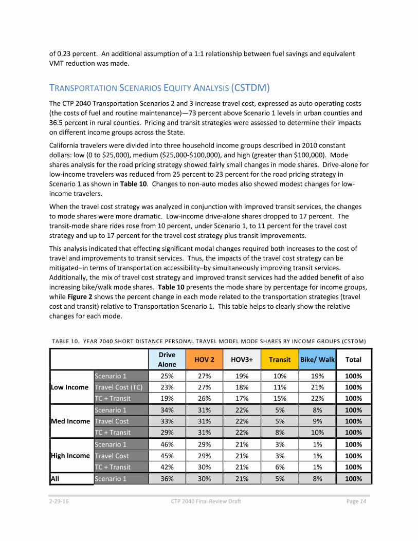
TRANSPORTATION SCENARIOS EQUITY ANALYSIS (CSTDM) The CTP 2040 Transportation Scenarios 2 and 3 increase travel cost, expressed as auto operating costs (the costs of fuel and routine maintenance)—73 percent above Scenario 1 levels in urban counties and 36.5 percent in rural counties. Pricing and transit strategies were assessed to determine their impacts on different income groups across the State.

California travelers were divided into three household income groups described in 2010 constant dollars: low (0 to $25,000), medium ($25,000-$100,000), and high (greater than $100,000). Mode shares analysis for the road pricing strategy showed fairly small changes in mode shares. Drive-alone for low-income travelers was reduced from 25 percent to 23 percent for the road pricing strategy in Scenario 1 as shown in Table 10. Changes to non-auto modes also showed modest changes for low-income travelers.

When the travel cost strategy was analyzed in conjunction with improved transit services, the changes to mode shares were more dramatic. Low-income drive-alone shares dropped to 17 percent. The transit-mode share rides rose from 10 percent, under Scenario 1, to 11 percent for the travel cost strategy and up to 17 percent for the travel cost strategy plus transit improvements.

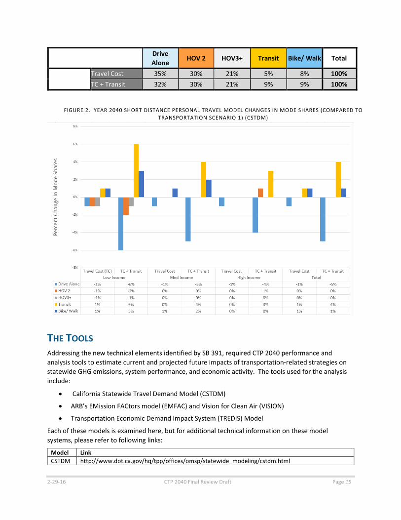
This analysis indicated that effecting significant modal changes required both increases to the cost of travel and improvements to transit services. Thus, the impacts of the travel cost strategy can be mitigated–in terms of transportation accessibility–by simultaneously improving transit services. Additionally, the mix of travel cost strategy and improved transit services had the added benefit of also increasing bike/walk mode shares. Table 10 presents the mode share by percentage for income groups, while Figure 2 shows the percent change in each mode related to the transportation strategies (travel cost and transit) relative to Transportation Scenario 1. This table helps to clearly show the relative changes for each mode.

TABLE 10. YEAR 2040 SHORT DISTANCE PERSONAL TRAVEL MODEL MODE SHARES BY INCOME GROUPS (CSTDM)

Drive Alone

HOV 2 HOV3+ Transit Bike/ Walk Total

Low Income Scenario 1 25% 27% 19% 10% 19% 100% Travel Cost (TC) 23% 27% 18% 11% 21% 100% TC + Transit 19% 26% 17% 15% 22% 100%

Med Income Scenario 1 34% 31% 22% 5% 8% 100% Travel Cost 33% 31% 22% 5% 9% 100% TC + Transit 29% 31% 22% 8% 10% 100%

High Income Scenario 1 46% 29% 21% 3% 1% 100% Travel Cost 45% 29% 21% 3% 1% 100% TC + Transit 42% 30% 21% 6% 1% 100%

All Scenario 1 36% 30% 21% 5% 8% 100%


Drive Alone HOV 2 HOV3+ Transit Bike/ Walk Total

Travel Cost 35% 30% 21% 5% 8% 100% TC + Transit 32% 30% 21% 9% 9% 100%

THE TOOLS Addressing the new technical elements identified by SB 391, required CTP 2040 performance and analysis tools to estimate current and projected future impacts of transportation-related strategies on statewide GHG emissions, system performance, and economic activity. The tools used for the analysis include:

• California Statewide Travel Demand Model (CSTDM)

• ARB’s EMission FACtors model (EMFAC) and Vision for Clean Air (VISION)

• Transportation Economic Demand Impact System (TREDIS) Model

Each of these models is examined here, but for additional technical information on these model systems, please refer to following links:

Model Link CSTDM http://www.dot.ca.gov/hq/tpp/offices/omsp/statewide_modeling/cstdm.html

FIGURE 2. YEAR 2040 SHORT DISTANCE PERSONAL TRAVEL MODEL CHANGES IN MODE SHARES (COMPARED TO TRANSPORTATION SCENARIO 1) (CSTDM)


EMFAC http://www.arb.ca.gov/emfac/ VISION http://www.arb.ca.gov/planning/vision/vision.htm TREDIS http://www.dot.ca.gov/hq/tpp/offices/osp/ctp2040/ctp2040_tac/oct_24_2013_tac_mtg/TREDIS_for

_Caltrans_October_2013_notes_bp.pdf

The following is a brief description of the tools, their individual functions, and how they contribute to the overall analysis. Figure 4 is a graphical representation of the modeling process and how information flows and interacts.

FIGURE 4. CTP 2040 MODELING PROCESS (CALTRANS)

CALIFORNIA STATEWIDE TRAVEL DEMAND MODEL12 The CSTDM is a multimodal, tour-based, travel demand model covering the entire State. It represents both personal and commercial travel, and incorporates the statewide networks for roads, rail, bus, and air travel. The 2012 California Household Travel Survey (CHTS) and the 2010 United States Census, along

- - - - - - - - - - - - - - - - - - - - - - - - - - - - - 12 http://www.dot.ca.gov/hq/tpp/offices/omsp/Statewide_modeling/cstdm.html

http://www.arb.ca.gov/emfac/

http://www.arb.ca.gov/planning/vision/vision.htm


with regional MPO SCS land use assumptions for population and employment were key inputs into the CSTDM Development. The CSTDM outputs a number of performance measures (VMT, VHD, trips, etc.) that are used in the subsequent emissions and economic benefit analyses.

EMISSIONS FACTOR MODEL13 The EMFAC model is used to assess emissions from on-road vehicles. The latest version of the model, EMFAC2014, was released in May 2015. The EMFAC2014 release is needed to support the ARB regulatory and air quality planning efforts and to meet the Federal Highway Administration (FHWA) transportation planning requirements. EMFAC2014 includes the latest data on California’s car and truck fleets and travel activity. The model also reflects the emission benefits of ARB’s recent rulemakings, including on-road diesel fleet rules, Pavley Clean Car Standards, and the Low-Carbon Fuel Standard.14 CSTDM outputs are then input to EMFAC2014 to calculate future transportation-related emissions for California. The EMFAC model addresses the emissions quantification of the vehicle activity from the CSTDM, as required by SB 391.

AIR RESOURCES BOARD VISION MODEL15 The ARB VISION model (VISION 2.0) is used for air quality and climate emissions planning. VISION evaluates strategies to meet California’s multiple air quality and climate change goals well into the future (to the year 2050). The model’s exploration of the technology and energy transformation needed to meet goals provides a foundation for future integrated air quality and climate change program development. VISION addresses future changes in vehicle technology, vehicle efficiency, alternative fuels, and activity changes, and evaluates their impacts on emissions above and beyond on-road diesel fleet rules, Advanced Clean Car Standards, and the Low-Carbon Fuel Standard required by SB 391.

Transportation Economic Development Impact System

TREDIS was developed by Economic Development Research Group, Inc. TREDIS is an integrated economic analysis system for transportation planning and project assessment and is designed to analyze the macroeconomic impacts of long-range plans such as the CTP 2040. TREDIS assesses costs, benefits, and economic impacts across a range of economic responses and societal perspectives of passenger and freight travel across all modes. TREDIS was used to assess the economic impacts from the CSTDM relating to passenger and short distance truck travel information. TREDIS addresses the economic forecasts from the vehicle activity of the CSTDM required by SB 391 for the CTP 2040.

- - - - - - - - - - - - - - - - - - - - - - - - - - - - - 13 http://www.arb.ca.gov/msei/msei.htm 14http://www.arb.ca.gov/msei/emfac2011-technical-documentation-final-updated-0712-v03.pdf 15 http://www.arb.ca.gov/planning/vision/vision.htm

http://www.arb.ca.gov/msei/msei.htm

http://www.arb.ca.gov/msei/emfac2011-technical-documentation-final-updated-0712-v03.pdf

http://www.arb.ca.gov/planning/vision/vision.htm


ARB VISION MODEL ARB prepared a technical memorandum summarizing final CTP 2040 EMFAC and VISION Model forecasts. That memorandum is included here in its entirety.

ARB MEMO

Air Quality Planning and Science Division California Air Resources Board

July 17, 2015

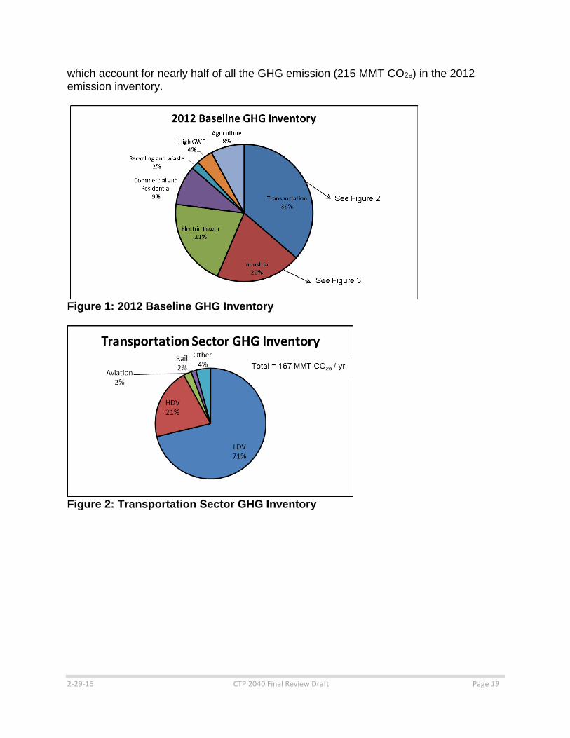
To: California Department of Transportation CTP 2040 Staff Subject: Updated ARB Vision CTP results for Alternatives 1, 2, and 3 Summary Updated results for CTP 2040 Alternatives 1, 2, and 3 have been completed. This report is an update to the previous report dated January 28, 2015. The baseline, Alternative 1, achieved a 3% reduction in GHG emissions by 2040, but shows an increase of 10% in 2050 over the 2020 base year. Alternative 2 reduced GHG emissions, with 23% and 15% reductions in 2040 and 2050 respectively below the Alternative 1 2020 base year, but still did not achieve an 80% reduction by 2050 (the target is 32 MMT CO2e for this analysis). Finally, Alternative 3 achieved an 80% reduction in 2050 achieving the GHG goal. Detailed analysis, input assumptions, and results are given below. Background For reference, Figure 1 below is a pie graph of the baseline GHG emission inventory for all sectors in calendar year 2012. Total GHG emissions in 2012 were estimated to be 461 MMT CO2e of which transportation accounted for 36% (167 MMT CO2e) and industrial emissions, which include refineries and oil and gas extraction, accounted for 20% (93 MMT CO2e) of the inventory. Figure 2 further breaks down the transportation section emissions, while Figure 3 expands the industrial section emissions. Figure 2 illustrates that on-road emissions from LDVs and HDVs account for 92% (154 MMT CO2e) of the transportation sector emissions with LDV contributing the greatest portion (72% or 120 MMT CO2e). From Figure 3, refineries and oil and gas extraction contribute ~50% of the industrial sector emissions (48 MMT CO2e). Adding the three sectors together, transportation, refineries, and oil and gas extraction, gives a wheel-to-wheel (WTW) perspective of the transportation sector total emissions occurring in California,


which account for nearly half of all the GHG emission (215 MMT CO2e) in the 2012 emission inventory.

Figure 1: 2012 Baseline GHG Inventory

Figure 2: Transportation Sector GHG Inventory


Figure 3: Industrial Sector GHG Inventory Methodology Scenarios were run for Caltrans Alternatives 1, 2, and 3 to determine total GHG emissions and fuel demand from 2010 to 2050. The sectors highlighted in this analysis, which were most relevant for CTP, were LDV, HDV, high-speed rail (HSR), aviation (intrastate), and rail (passenger and freight). The ARB Vision 2.0 model was used for the analysis and other transportation sectors (ocean going vessels, harbor craft, cargo handling equipment, and off-road vehicles) lumped together under “other transportation” emissions. Vision 2.0 incorporates the latest data from ARB’s EMFAC 2014 as well as the newest baseline policy assumptions for other sectors. Updated LDV and HDV activity data were supplied to ARB from the Caltrans CSTDM model, which gave VMT by speed bin for three select years (2010, 2020, and 2040)16. Table 1 below displays total VMT in billions of miles for Alternative 1 in 2010, 2020 and 2040 and the 2040 VMT for the other two Alternatives. Also shown in the table is the percent reduction in VMT between Alternatives 1 and 2 (3 is the same VMT as 2). Note that VMT was reduced by 28% in 2040 for Alternative 2 and Alternative 3. ARB extrapolated VMT annually for years between 2010 and 2040. Beyond 2040, VMT growth rates from EMFAC 2014 were applied to the 2040 data point.

Table 1: Total VMT from CSTDM for Alternatives 1, 2 and 3 in billions of miles per year

2010 2020 2040 Alternative 1

LDV 189.7 208 265 HDV 74 73.5 88 Total 264 282 353

- - - - - - - - - - - - - - - - - - - - - - - - - - - - - 16 Updated 2020 and 2040 activity data were received on June 11, 2015 by email from Cambridge Systematics, Inc., Revised

2040 activity data were received on July 10, 2015.


Alternatives 2 and 3 LDV - - 181 HDV - - 73 Total - - 254 % Reduction 28%

Inputs for HSR came from the HSR Authority High-Speed Rail plan, which gives LDV VMT offsets and intrastate aviation trip reductions. HSR authority assumes that HSR will be entirely powered by renewable electricity so there are no GHG emissions associated with HSR and HSR only affects VMT and aircraft trips. For conventional passenger rail, inputs were matched to Vision 2.0 and the Caltrans rail plan for Alternative 1. Ridership was assumed to double for Alternative 2. It was assumed that there were no aircraft fuel efficiency improvements for Alternatives 1 and 2, but HSR aircraft trip reductions were included for both alternatives. Finally, all other assumptions, including the off-road sectors, came from the ARB Vision 2.0 baseline scenario (projections of existing policies and sector growth estimates). In order to achieve the 2050 GHG target, additional assumptions were made for Alternative 3 in ARB Vision 2.0 for the following sectors. For LDVs, the assumptions are that fuel efficiency increases such that new vehicle fuel efficiency is four times higher by 2050 from today’s levels and an assumption of ~20 million LDV ZEVs on the road in 2050. For HDVs, the assumptions are that fuel efficiency is more than 50% higher by 2030 for new vehicles and ZEVs (BEV, FCV) will represent 12% of total sales by 2030. For freight rail and aviation, the assumptions are that fuel efficiency increases by 2.0% per year starting in 2015. Assumptions for HSR and conventional passenger rail remained the same as in Alternative 2. For transportation fuels, this analysis assumes 7 ”BGGE” bio-fuels are available, including drop-in renewable fuel, by 2050 (~1 BGGE in Alternative 1). Also assumed is a 75% renewable electricity and hydrogen supply mix by 2050 as compared to 33% for both in Alternative 1 (for years 2020-2050). Alternatives 1 and 2 Results Results shown in Tables 2 and 3 below are for Alternatives 1 and 2, respectively. The table displays total fuel demand (quadrillion BTUs or “quads” and “BGGE”), GHG emissions (MMT CO2e / yr), and relative percent reduction below Alternative 1 2020 for 2040 and 2050.


Table 2: Alternative 1 Results Alternative 1

2010 2012 2020 2040 2050 Fuel Demand (Quads)

Gasoline (CaRFG)1 1.31 1.25 1.10 0.80 0.90

Diesel (ULSD)2 0.61 0.61 0.69 0.92 1.07 Jet Fuel 0.47 0.46 0.51 0.68 0.77 Electric Power 0.000 0.001 0.008 0.027 0.036 Hydrogen 0.000 0.000 0.001 0.008 0.010

Fuel Demand (BGGE) Gas 11.7 11.1 9.8 7.1 8.0 Diesel 5.5 5.5 6.2 8.2 9.5 Jet Fuel 4.2 4.1 4.6 6.1 6.9 Electric Power 0.00 0.01 0.07 0.25 0.33 Hydrogen 0.00 0.00 0.01 0.07 0.09

GHG Emissions (MMT CO2e / yr) LDV + Bus 114 108 94 70 79 HDV 50 49 50 63 69 Rail 2 3 3 5 6 Aviation 4 4 5 6 7 Other Transportation 4 4 6 10 14 Total 175 168 158 154 175 Target - - - - 32

GHG Relative Reduction Below Alternative 1 20203 (%) LDV + Bus - - - 26% 17% HDV - - - -26% -38% Rail - - - -53% -91% Aviation - - - -26% -40% Other Transportation - - - -70% -129% Total - - - 3% -10% Target - - - - 80%

1California Reformulated Gasoline (CaRFG) includes 10% ethanol blended by volume 2Diesel includes 5% biodiesel by volume 3AB 32 requires that the 2020 total GHG inventory is the same as the 1990 GHG inventory, while the law does not require that each individual sector achieve its absolute 1990 value. Because the CTP project does not include all sectors, it is assumed that the transportation sector 2020 GHG value calculated for Alternative 1 will be the reference point for the 2050 GHG reductions.


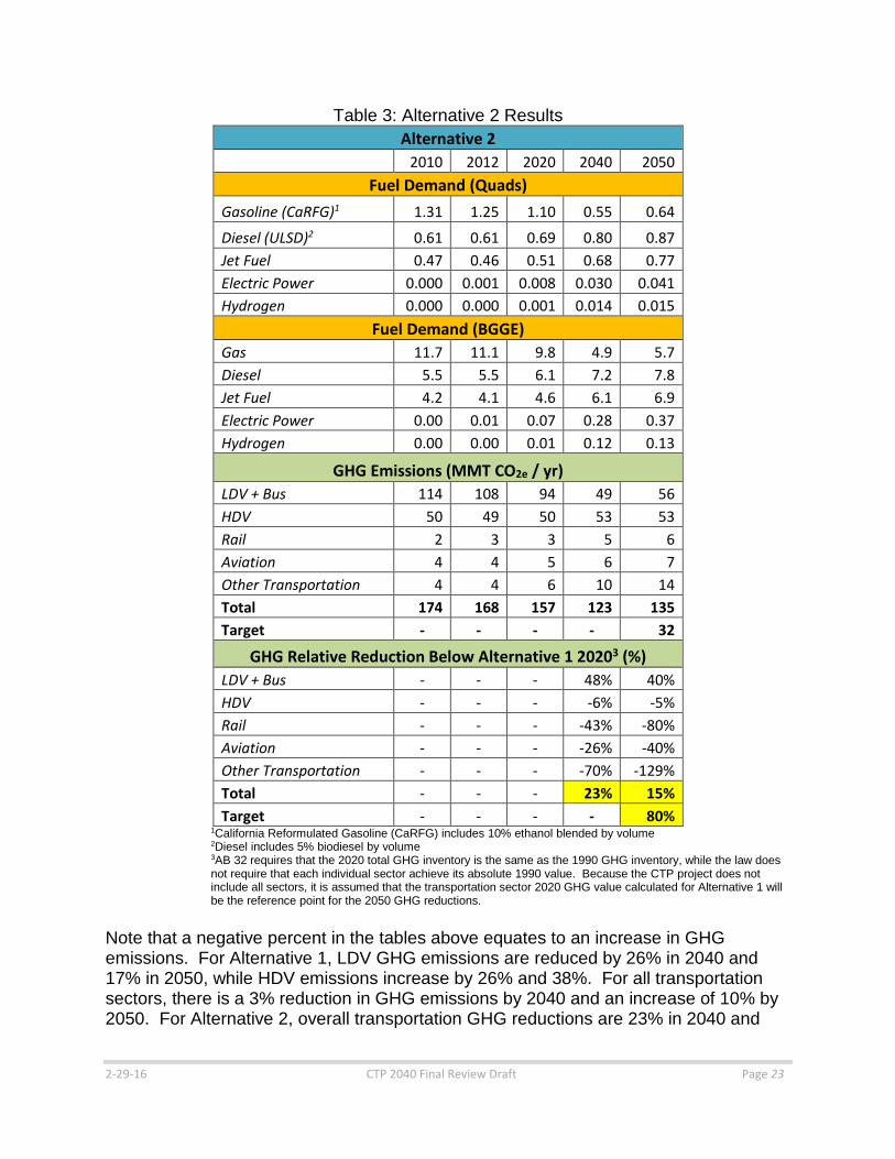
Table 3: Alternative 2 Results Alternative 2

2010 2012 2020 2040 2050 Fuel Demand (Quads)

Gasoline (CaRFG)1 1.31 1.25 1.10 0.55 0.64




GHG Relative Reduction Below Alternative 1 20203 (%) LDV + Bus - - - 48% 40% HDV - - - -6% -5% Rail - - - -43% -80% Aviation - - - -26% -40% Other Transportation - - - -70% -129% Total - - - 23% 15% Target - - - - 80%


Note that a negative percent in the tables above equates to an increase in GHG emissions. For Alternative 1, LDV GHG emissions are reduced by 26% in 2040 and 17% in 2050, while HDV emissions increase by 26% and 38%. For all transportation sectors, there is a 3% reduction in GHG emissions by 2040 and an increase of 10% by 2050. For Alternative 2, overall transportation GHG reductions are 23% in 2040 and


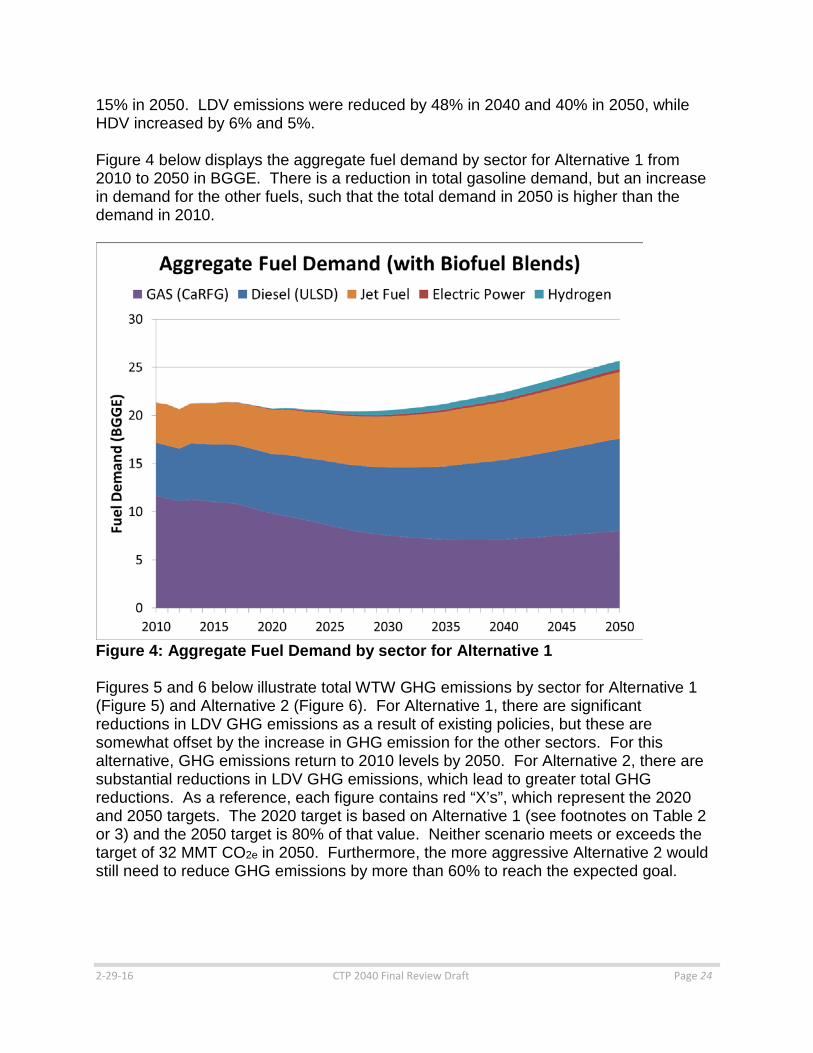
15% in 2050. LDV emissions were reduced by 48% in 2040 and 40% in 2050, while HDV increased by 6% and 5%. Figure 4 below displays the aggregate fuel demand by sector for Alternative 1 from 2010 to 2050 in BGGE. There is a reduction in total gasoline demand, but an increase in demand for the other fuels, such that the total demand in 2050 is higher than the demand in 2010.

Figure 4: Aggregate Fuel Demand by sector for Alternative 1 Figures 5 and 6 below illustrate total WTW GHG emissions by sector for Alternative 1 (Figure 5) and Alternative 2 (Figure 6). For Alternative 1, there are significant reductions in LDV GHG emissions as a result of existing policies, but these are somewhat offset by the increase in GHG emission for the other sectors. For this alternative, GHG emissions return to 2010 levels by 2050. For Alternative 2, there are substantial reductions in LDV GHG emissions, which lead to greater total GHG reductions. As a reference, each figure contains red “X’s”, which represent the 2020 and 2050 targets. The 2020 target is based on Alternative 1 (see footnotes on Table 2 or 3) and the 2050 target is 80% of that value. Neither scenario meets or exceeds the target of 32 MMT CO2e in 2050. Furthermore, the more aggressive Alternative 2 would still need to reduce GHG emissions by more than 60% to reach the expected goal.


Figure 5: WTW GHG Emissions by Sector for Alternative 1

Figure 6: WTW GHG Emissions by Sector for Alternative 2


Alternative 3 Results Results are shown in Table 4 below for Alternative 3. The table displays total fuel demand (quadrillion BTUs or “quads” and billions gallons gasoline equivalent or “BGGE”), GHG emissions (MMT CO2e / yr), and relative percent reduction below 2020 for 2040 and 2050.

Table 4: Alternative 3 Results

Alternative 3 2010 2012 2020 2040 2050

Fuel Demand (Quads) Gasoline (CaRFG)1 1.31 1.25 1.10 0.33 0.17




GHG Relative Reduction Below Alternative 1 20203 (%) LDV + Bus - - - 72% 88% HDV - - - 46% 76% Rail - - - 13% 22% Aviation - - - 52% 62% Other Transportation - - - 12% 28% Total - - - 60% 80% Target - - - - 80%



For Alternative 3, LDV GHG emissions are reduced by 72% in 2040 and 88% in 2050, while HDV emissions decrease by 46% and 76%. For all transportation sectors, there is a 60% reduction in GHG emissions by 2040 and 80% reduction by 2050. Figure 7 below displays the aggregate fuel demand by sector for Alternative 3 from 2010 to 2050. There is a large reduction in total demand due to the decrease in gasoline demand and the decrease in demand for the other sectors, such that the total demand in 2050 is 24% lower than the base value in 2010. Figure 7: Aggregate Fuel Demand by sector for Alternative 3 Figure 8 below illustrates the total WTW GHG emissions by sector for Alternative 3. There are significant reductions in LDV GHG emissions as well as reductions in the other transportation sectors such that this Alternative meets the target of 32 MMT CO2e. As a reference, the figure contains red “X’s”, which represent the 2020 and 2050 targets (see explanation above).

Figure 8: WTW GHG Emissions by Sector for Alternative 3 Conclusions The 2050 GHG target for CTP2040 is 80% below the 2020 data point for Alternative 1, or a target of approximately 32 MMT CO2e for the entire transportation sector, to meet its “equal share” of the GHG emissions target. Neither Alternative 1 nor 2 attained this


target for the entire transportation sector. In Alternative 2, the LDV sector was the only sector to reduce emissions but barely reached 40% of its “equal share” target. In Alternative 3, the LDV mode attained more than its equal share and the other sectors reduced emissions significantly such that the 2050 target was obtained. It’s important to note that the official full statewide GHG Inventory 2050 target equals 86 MMT CO2e for all sectors, with many of those sectors likely unable to reach their equal share, such that the transportation sector may have to reduce beyond their equal share. Comment on Methodology CSTDM has not been fully validated against official State records for gasoline, diesel, and jet fuel consumption in the 2010 base year demand.


ECONOMIC IMPACT ANALYSIS OF CTP 2040 The CTP is the first long-range planning document to consider the economic impacts of implementing the concepts and strategies presented. SB 391 requires the CTP to address how the State will achieve maximum feasible emissions reductions to attain a statewide decrease of GHG emissions as outlined in AB 32 (1990 levels by 2020 and 80 percent below 1990 levels by 2050). Under SB 391, the CTP is required to include a policy element consisting of the Department’s policy and system performance objectives, a strategy element that includes concepts and strategies developed in the plan, and incorporating concepts in adopted RTPs. Additionally, the CTP must include an element that integrates economic forecasts and recommendations for achieving the concepts and strategies presented. The CTP is also required to address certain subject areas identified in SB 391 and U.S. Code 23 USC 134 and 135 of the U.S. Code, Title 23, Chapter 1, Federal-Aid Highways. SB 391 codifies consideration of “Economic Development, including productivity and efficiency” and U.S. Code specifies that the planning process provide consideration of projects and strategies that will: 1) support the economic vitality of the metropolitan area, especially by enabling global competitiveness, productivity, and efficiency, and 2) promote consistency between transportation improvements and State and local planned growth and economic development patterns. However, SB 391 excludes the inclusion of projects in the CTP.

In previous CTP documents, economic consideration was limited to identifying the impacts associated with financial investments in transportation infrastructure projects and discussing transportation dependent industries. Input-Output (I-O) models are commonly used to assess the potential economic impacts of transportation infrastructure projects. Investments in transit and highway infrastructure projects translate into short-term increases in jobs, incomes and output (GSP). I-O models use multipliers that simulate spending patterns within and among industries resulting from initial transportation infrastructure investments. The outcomes are generally regarded as annual impacts, though research indicates these investments can have long-term impacts. Another matrix used in the past is the number of jobs in travel related industries. The North American Industry Classification System (NAICS) reports transportation related jobs in nearly all major industry categories reflecting the wide span of impact.

Economic consideration in the CTP 2040, unlike previous documents, incorporates a more comprehensive analysis. Caltrans’ Economic Analysis Branch (EAB) utilized the TREDIS model to evaluate the wider economic impacts of proposed transportation investment and policy strategies identified in the CTP 2040. TREDIS is an integrated economic impact and analysis tool covering a range of applications including benefits, costs, finance and macroeconomic impacts. The emphasis of the CTP 2040 analysis focused on the impacts of travel costs, market access and economic adjustments. The travel cost impacts on households and industries are evaluated for their spending and productivity impacts. Cost savings, or dis-savings, from transportation investments or policy decisions translate into changes in household spending patterns and productivity impacts on industries. TREDIS measures how households and industries respond to changes in travel due to investment and policy changes. Additionally, TREDIS evaluates the direct changes in productivity or regional economic activity beyond the change in travel times or travel costs for users of the transportation network. These include increased production from business migration, increased labor productivity from agglomeration economies and increased international exports from improved access to international gateways.


LIMITATIONS The economic impact analysis completed for the CTP 2040 meets the requirements set in SB 391. The results of the analysis are limited to the long-term economic impacts of traveler (time and costs) savings and market access changes, specifically, efficiency and productivity. The analysis does not include key considerations such as land use and transportation infrastructure expenditure impacts. Each of these components alone could have significant economic impacts. Limitation in the capacity of the CSTDM to address land use impacts prohibits consideration in the economic analysis. Land use is considered in the CSTDM outputs only so far as they are included in the Scenario 1 development. The impacts from expenditures related to infrastructure improvements were omitted since the CTP 2040 does not, by law, identify or consider individual projects. This document and the analysis, features transportation policy recommendations and their impacts.

Finally, limitations exist from the application of the CSTDM and the interpretation of the results. For instance, the CSTDM assigns transit, bicycle and pedestrian trips, but does not apply distance or time traveled as it does for passenger and commercial vehicles. From an economic assessment point of view, travel savings is difficult to assess. For this analysis, distance and time of travel were estimated based on the 2013 CHTS.

appendix 7 technical analysis - caltrans · appendix 7 . technical analysis . 2-29-16 ctp 2040...

Documents