analytical tools for the performance evaluation of wireless
TRANSCRIPT
'
&
$
%
Analytical Tools for the Performance Evaluationof Wireless Communication Systems
Mohamed-Slim Alouini
Department of Electrical and Computer Engineering
University of Minnesota
Minneapolis, MN 55455, USA.
E-mail: <[email protected]>
Communication & Coding Theory for Wireless Channels
Norwegian University of Science and Technology (NTNU)
Trondheim, Norway.
October 2002.

'
&
$
%
Outline - Part I: Some Basics
1. Introduction: Background, Motivation, and Goals.
2. Fading Channels Characterizationand Modeling (Brief Overview)
•Multipath Fading
• Shadowing
3. Single Channel Reception
• Outage Probability
• Average Fade/Outage Duration (AFD or AOD)
• Average Probability of Error or AverageError Rate
– Coherent Detection
– Differentially Coherent and NoncoherentDetection

'
&
$
%
Design of Wireless Comm. Systems
• Often the basic problem facing the wireless sys-tem designer is to determine the “best” schemein the face of his or her available constraints.
• An informed decision/choice relies on an accu-rate quantitative performance evaluation andcomparison of various options and techniques.
• Performance of wireless communication systemscan be measured in terms of:
– Outage probability.
– Average outage/fade duration.
– Average bit or symbol error rate.

'
&
$
%
Performance Analysis
• Can lead to closed-form expressions or tractablesolutions
– Insight into performance limits and perfor-mance dependence on system parameters ofinterest.
– A significant speed-up factor relative tocomputersimulations or field tests/experiments.
– Quantify the tradeoff between performanceand complexity.
– Useful background study for accurate systemdesign, improvement, and optimization.
• Approach
– Mathematical and statistical modeling.
– Analytical derivations.
– Exact or approximate expressions in com-putable forms.
– Numerical examples and design guidelines.
'
&
$
%
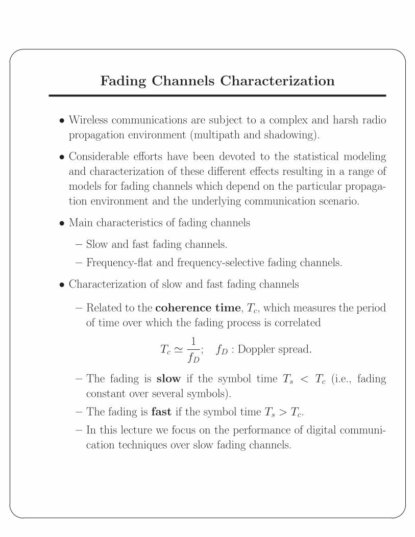
Fading Channels Characterization
• Wireless communications are subject to a complex and harsh radio
propagation environment (multipath and shadowing).
• Considerable efforts have been devoted to the statistical modeling
and characterization of these different effects resulting in a range of
models for fading channels which depend on the particular propaga-
tion environment and the underlying communication scenario.
• Main characteristics of fading channels
– Slow and fast fading channels.
– Frequency-flat and frequency-selective fading channels.
• Characterization of slow and fast fading channels
– Related to the coherence time, Tc, which measures the period
of time over which the fading process is correlated
Tc ' 1
fD; fD : Doppler spread.
– The fading is slow if the symbol time Ts < Tc (i.e., fading
constant over several symbols).
– The fading is fast if the symbol time Ts > Tc.
– In this lecture we focus on the performance of digital communi-
cation techniques over slow fading channels.

'
&
$
%
• Characterization of frequency-flat and frequency-selective channels.
– Related to the multipath intensity profile (MIP) or power
delay profile (PDP) φc(τ ).
– Delay spread or multipath spread Tm is the maximum
value of τ beyond which φc(τ ) ' 0.
– Coherence bandwidth is defined as
∆fc ' 1
Tm
– Frequency-flat or Frequency non-selective fading
∗ Signal components with frequency separation (∆f ) << (∆f )care completely correlated (affected in the same way by chan-
nel).
∗ Typical of narrowband signals.
∗ Since multipath delays are small compared to transmission
baud interval, signal is not distorted (only attenuated) by the
channel.
– Nonflat fading or Frequency-selective fading
∗ Signal components with frequency separation (∆f ) >> (∆f )care weakly correlated (affected differently by channel).
∗ Typical of wideband signals (e.g. spread-spectrum signals).
∗ Since multipath delays are large compared to transmission
baud interval, signal is severely distorted (not only attenu-
ated) by the channel.

'
&
$
%
Modeling of Frequency-Flat Fading Channels
• The received carrier amplitude is modulated by the random fading
amplitude α
– Ω = α2: average fading power of α.
– pα(α): probability density function (PDF) of α.
• Let us denote the instantaneous signal-to-noise power ratio (SNR)
per symbol by γ = α2Es/N0 and the average SNR per symbol by
γ = ΩEs/N0, where Es is the energy per symbol.
• A standard transformation of the PDF pα(α) yields
pγ(γ) =pα
(√Ω γγ
)
2√
γγΩ
.
• Various statistical models
– Multipath fading models
∗ Rayleigh.
∗ Nakagami-q (Hoyt).
∗ Nakagami-n (Rice).
∗ Nakagami-m.
– Shadowing model
∗ Log-normal.
– Composite multipath/shadowing models.
∗ Composite Nakagami-m/Log-normal.

'
&
$
%
Multipath Fading
• Rayleigh model
– PDF of fading amplitude given by
pα(α; Ω) =2 α
Ωexp
(−α2
Ω
); α ≥ 0,
– The instantaneous SNR per symbol of the channel, γ, is dis-
tributed according to an exponential distribution
pγ(γ; γ) =1
γexp
(−γ
γ
); γ ≥ 0.
– Agrees very well with experimental data for multipath propaga-
tion where no line-of-sight (LOS) path exists between the trans-
mitter and receiver antennas.
– Applies to macrocellular radio mobile systems as well as to tropo-
spheric, ionospheric, and maritime ship-to-ship communication.
• Nakagami-q (Hoyt) model
– PDF of fading amplitude given by
pα(α; Ω, q) =(1 + q2) α
q Ωexp
(−(1 + q2)2 α2
4q2Ω
)I0
((1− q4)α2
4 q2Ω
); α ≥ 0,
where I0(.) is the zero-th order modified Bessel function of the
first kind, and q is the Nakagami-q fading parameter which ranges
from 0 (half-Gaussian model) to 1 (Rayleigh model).
'
&
$
%
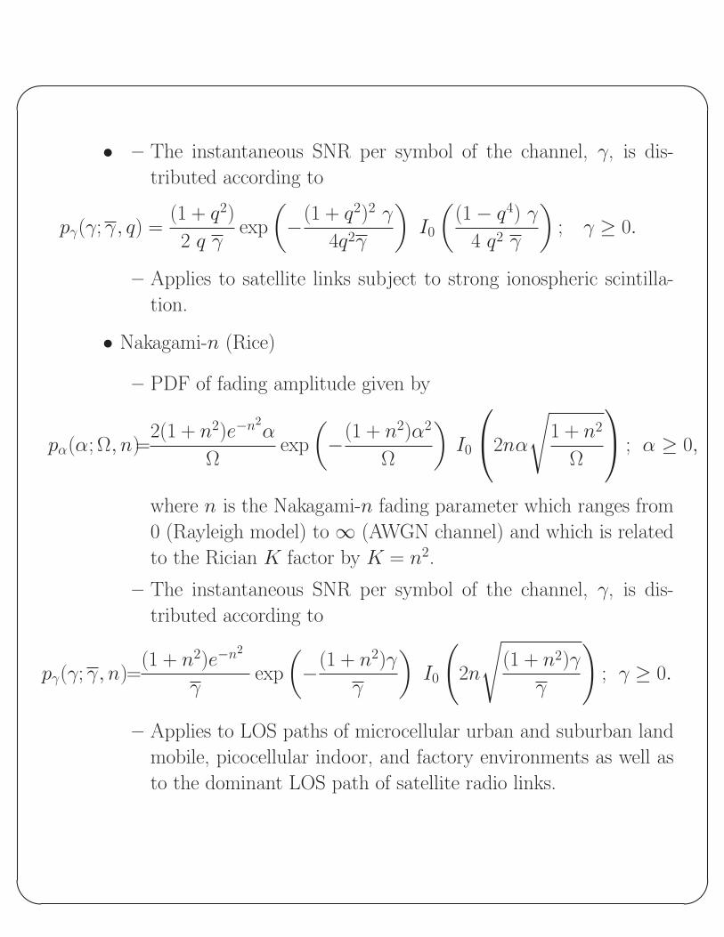
• – The instantaneous SNR per symbol of the channel, γ, is dis-
tributed according to
pγ(γ; γ, q) =(1 + q2)
2 q γexp
(−(1 + q2)2 γ
4q2γ
)I0
((1− q4) γ
4 q2 γ
); γ ≥ 0.
– Applies to satellite links subject to strong ionospheric scintilla-
tion.
• Nakagami-n (Rice)
– PDF of fading amplitude given by
pα(α; Ω, n)=2(1 + n2)e−n2
α
Ωexp
(−(1 + n2)α2
Ω
)I0
2nα
√1 + n2
Ω
; α ≥ 0,
where n is the Nakagami-n fading parameter which ranges from
0 (Rayleigh model) to ∞ (AWGN channel) and which is related
to the Rician K factor by K = n2.
– The instantaneous SNR per symbol of the channel, γ, is dis-
tributed according to
pγ(γ; γ, n)=(1 + n2)e−n2
γexp
(−(1 + n2)γ
γ
)I0
(2n
√(1 + n2)γ
γ
); γ ≥ 0.
– Applies to LOS paths of microcellular urban and suburban land
mobile, picocellular indoor, and factory environments as well as
to the dominant LOS path of satellite radio links.

'
&
$
%
• Nakagami-m
– PDF of fading amplitude given by
pα(α; Ω,m) =2 mm α2m−1
Ωm Γ(m)exp
(−m α2
Ω
); α ≥ 0,
where m is the Nakagami-m fading parameter which ranges from
1/2 (half-Gaussian model) to ∞ (AWGN channel).
– The instantaneous SNR per symbol of the channel, γ, is dis-
tributed according to a gamma distribution:
pγ(γ; γ, m) =mm γm−1
γm Γ(m)exp
(−m γ
γ
); γ ≥ 0.
– Closely approximate the Nakagami-q (Hoyt) and the Nakagami-n
(Rice) models.
– Often gives the best fit to land-mobile and indoor-mobile multi-
path propagation, as well as scintillating ionospheric radio links.

'
&
$
%
Nakagami-m PDF
0 0.5 1 1.5 2 2.50
0.2
0.4
0.6
0.8
1
1.2
1.4
1.6
1.8
2The Nakagami PDF for Different Values of the Nakagami Fading Parameter m
C hanne l Fade A mp litude α
Pro
ba
bili
ty D
en
sit
y F
un
ctio
n P
α(α
)
m=1/2
m=1
m=2
m=4
Figure 1: The Nakagami PDF for different values of the Nakagami fading parameter m.
'
&
$
%
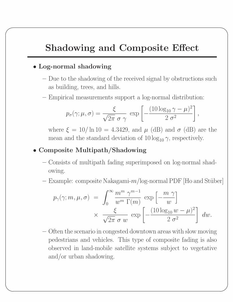
Shadowing and Composite Effect
• Log-normal shadowing
– Due to the shadowing of the received signal by obstructions such
as building, trees, and hills.
– Empirical measurements support a log-normal distribution:
pσ(γ; µ, σ) =ξ√
2π σ γexp
[−(10 log10 γ − µ)2
2 σ2
],
where ξ = 10/ ln 10 = 4.3429, and µ (dB) and σ (dB) are the
mean and the standard deviation of 10 log10 γ, respectively.
• Composite Multipath/Shadowing
– Consists of multipath fading superimposed on log-normal shad-
owing.
– Example: composite Nakagami-m/log-normal PDF [Ho and Stuber]
pγ(γ; m, µ, σ) =
∫ ∞
0
mm γm−1
wm Γ(m)exp
[−m γ
w
]
× ξ√2π σ w
exp
[−(10 log10 w − µ)2
2 σ2
]dw.
– Often the scenario in congested downtown areas with slow moving
pedestrians and vehicles. This type of composite fading is also
observed in land-mobile satellite systems subject to vegetative
and/or urban shadowing.

'
&
$
%
Modeling of Frequency-SelectiveFading Channels
• Frequency-selective fading channels can be modeled by a linear fil-
ter characterized by the following complex-valued lowpass equivalent
impulse response
h(t) =
Lp∑
l=1
αl e−jθl δ(t− τl),
where
– δ(.) is the Dirac delta function.
– l is the path index.
– Lp is the number of propagation paths and is related to the ratio
of the delay spread to the symbol time duration.
– αlLp
l=1, θlLp
l=1, and τlLp
l=1 are the random channel amplitudes,
phases, and delays, respectively.
• The fading amplitude αl of the lth “resolvable” path is assumed to be
a random variable with average fading power α2l denoted by Ωl and
with PDF pαl(αl) which can follow any one of the models presented
above.
• The ΩlLp
l=1 are related to the channel’s power delay profile or multi-
path intensity profile and which is typically a decreasing function of
the delay. Example: exponentially decaying profile for indoor office
buildings and congested urban areas:
Ωl = Ω1 e−τl/Tm; l = 1, 2, · · · , Lp,
where Ω1 is the average fading power corresponding to the first (ref-
erence) propagation path.
'
&
$
%
Outage Probability and Outage Duration
• Outage Probability
– Usually defined as the probability that the instantaneous bit error
rate (BER) exceeds a certain target BER.
– Equivalently it is the probability that the instantaneous SNR γ
falls below a certain target SNR γth:
Pout(γth) = Prob[γ ≤ γth] =
∫ γth
0
pγ(γ) dγ = Pγ(γth),
where Pγ(·) is the SNR cumulative distribution function (CDF).
• Average Outage Duration
– Usually defined as the average time that the instantaneous BER
remains above a certain target BER once it exceeds it.
– Equivalently it is the average time that the instantaneous SNR
γ(t) remains below a certain target SNR γth once it drops below
it:
T (γth) =Pout(γth)
N(γth),
where N(γth) is the average (up-ward or down-ward) crossing
rate of γ(t) at level γth.

'
&
$
%
Examples for CDFs of the SNR
• Rayleigh fading
Pγ(γ) = 1− e−γγ .
• Nakagami-n (Rice with K = n2) fading
Pγ(γ) = 1−Q
n
√2,
√2(1 + n2)
γγ
,
where Q(·, ·) is the Marcum Q-function traditionally defined by
Q(a, b) =
∫ ∞
b
x exp
(−x2 + a2
2
)I0(ax) dx.
• Nakagami-m fading
Pγ(γ) = 1−Γ
(m, m
γ γ)
Γ(m),
where Γ(·, ·) is the complementary incomplete gamma function tra-
ditionally defined by
Γ(α, x) =
∫ ∞
x
e−t tα−1 dt.
'
&
$
%
Average Bit Error Rate
• Average bit or symbol error rate.
– Coherent Detection
∗ Conditional (on the instantaneous SNR) BER for BPSK for
example
Pb(E/γ) = Q(√
2γ)
,
where Q(·) is the Gaussian Q-function traditionally defined
by
Q(x) =1√2π
∫ ∞
x
e−t2/2 dt.
∗ Average BER
Pb(E) =
∫ ∞
0
Pb(E/γ) pγ(γ) dγ.
– Differentially Coherent and Noncoherent Detection
∗ Conditional (on the instantaneous SNR) BER for DPSK for
example
Pb(E/γ) =1
2e−γ,
∗ Average BER of DPSK
Pb(E) =
∫ ∞
0
Pb(E/γ) pγ(γ) dγ =1
2Mγ(−1),
where Mγ(s) = Eγ[esγ] is the moment generating function
(MGF) of the SNR.
'
&
$
%
Examples for MGFs of the SNR
• Rayleigh fading
Mγ(s) = (1− sγ)−1.
• Nakagami-n (Rice with K = n2) fading
Mγ(s) =1 + n2
1 + n2 − sγexp
(sγn2
1 + n2 − sγ
).
• Nakagami-m fading
Mγ(s) =
(1− sγ
m
)−m
.
• Composite Nakagami-m/log-normal fading
Mγ(s) ' 1√π
Np∑n=1
Hxn
(1− s
10(√
2 σ xn+µ)/10
m
)−m
,
where
– Np is the order of the Hermite polynomial, HNp(.). Setting Np
to 20 is typically sufficient for excellent accuracy.
– xn are the zeros of the Np-order Hermite polynomial.
– Hxn are the weight factors of the Np-order Hermite polynomial.

'
&
$
%
Outline - Part II: Diversity Systems
1. Introduction: Concept, Intuition, and Notations.
2. Classification of Diversity Combining Techniques
3. Receiver Diversity Techniques
• “Pure” Diversity Combining Techniques
– Maximal-Ratio Combining (MRC)
– Equal Gain Combining (EGC)
– Selection Combining (SC)
– Switched and Stay Combining (SSC) and Switch-and-Examine
Combining (SEC)
• “Hybrid” Diversity Combining Techniques
– Generalized Selection Combining (GSC) and Generalized Switch-
and-Examine Combining (SEC)
– Two-Dimensional Diversity Schemes
4. Impact of Correlation on the Performance of Diversity Systems
5. Transmit Diversity Systems
6. Multiple-Input-Multiple-Output (MIMO) Systems
'
&
$
%
Diversity Combining
• Concept
– Diversity combining consists of:
∗ Receiving redundantly the same information bearing signal
over 2 or more fading channels.
∗ Combining these multiple replicas at the receiver in order to
increase the overall received SNR.
• Intuition
– The intuition behind diversity combining is to take advantage of
the low probability of concurrence of deep fades in all the diversity
branches to lower the probability of error and outage.
• Means of Realizing Diversity
– Multiple replicas can be obtained by extracting the signals via
different radio paths:
∗ Space: Multiple receiver antennas (antenna or site diversity).
∗ Frequency: Multiple frequency channels which are separated
by at least the coherence bandwidth of the channel (frequency
hopping or multicarrier systems).
∗ Time: Multiple time slots which are separated by at least the
coherence time of the channel (coded systems).
∗ Multipath: Resolving multipath components at different de-
lays (direct-sequence spread-spectrum systems with RAKE
reception).
'
&
$
%
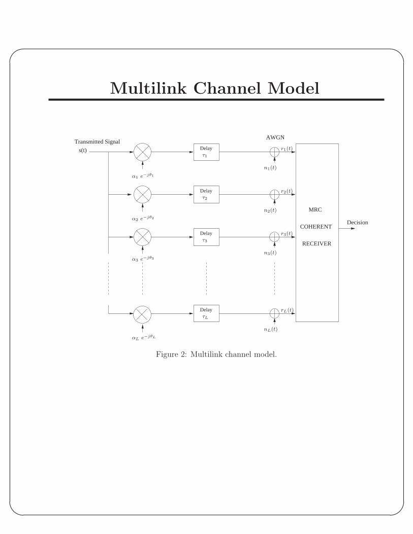
Multilink Channel Model
Delay
Delay
Delay
Delay
s(t)
Transmitted Signal
Decision
MRC
COHERENT
RECEIVER
AWGN
α1 e−jθ1
α2 e−jθ2
α3 e−jθ3
τ1
τ3
τ2
αL e−jθL
τL
n1(t)
n2(t)
nL(t)
n3(t)
r1(t)
r2(t)
r3(t)
rL(t)
Figure 2: Multilink channel model.
'
&
$
%
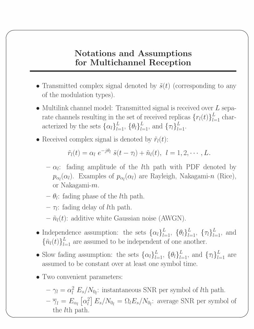
Notations and Assumptionsfor Multichannel Reception
• Transmitted complex signal denoted by s(t) (corresponding to any
of the modulation types).
• Multilink channel model: Transmitted signal is received over L sepa-
rate channels resulting in the set of received replicas rl(t)Ll=1 char-
acterized by the sets αlLl=1, θlL
l=1, and τlLl=1.
• Received complex signal is denoted by rl(t):
rl(t) = αl e−jθl s(t− τl) + nl(t), l = 1, 2, · · · , L.
– αl: fading amplitude of the lth path with PDF denoted by
pαl(αl). Examples of pαl
(αl) are Rayleigh, Nakagami-n (Rice),
or Nakagami-m.
– θl: fading phase of the lth path.
– τl: fading delay of lth path.
– nl(t): additive white Gaussian noise (AWGN).
• Independence assumption: the sets αlLl=1, θlL
l=1, τlLl=1, and
nl(t)Ll=1 are assumed to be independent of one another.
• Slow fading assumption: the sets αlLl=1, θlL
l=1, and τlLl=1 are
assumed to be constant over at least one symbol time.
• Two convenient parameters:
– γl = α2l Es/N0l
: instantaneous SNR per symbol of lth path.
– γl = Eαl
[α2
l
]Es/N0l
= ΩlEs/N0l: average SNR per symbol of
the lth path.

'
&
$
%
Classification of Diversity Systems
• Macroscopic versus microscopic diversity:
1. Macroscopic diversity mitigates the effect of shadowing.
2. Microscopic diversity mitigates the effect of multipath fading.
• “Soft” versus “Hard” diversity schemes:
1. Soft diversity combining schemes deal with signals.
2. Hard diversity combining schemes deal with bits.
• Receive versus transmit diversity schemes:
1. In receive diversity systems, the diversity is extracted at the re-
ceiver (for example multiple antennas deployed at the receiver).
2. In transmit diversity systems, the diversity is initiated at the
transmitter (for example multiple antennas deployed at the trans-
mitter).
3. MIMO systems, such as systems with multiple antennas at the
transmitter and the receiver, take advantage of diversity at both
the receiver and transmitter ends.
• Pre-detection versus post-detection combining:
1. Pre-detection combining: diversity combining takes place before
detection.
2. Post-detection combining: diversity combining takes place after
detection.

'
&
$
%
Diversity Combining Techniques
• Four “pure” types of diversity combining techniques:
– Maximal-ratio combining (MRC)
∗ Optimal scheme but requires knowledge of all channel pa-
rameters (i.e., fading amplitude and phase of every diversity
path).
∗ Used with coherent modulations.
– Equal gain combining (EGC)
∗ Coherent version limited in practice to constant envelope mod-
ulations.
∗ Noncoherent version optimum in the maximum-likelihood sense
for i.i.d. Rayleigh channels.
– Selection combining (SC)
∗ Uses the diversity path/branch with the best quality.
∗ Requires simultaneous and continuous monitoring of all diver-
sity branches.
– Switched (or scanning diversity)
∗ Two variants: Switch-and-stay combining (SSC) and switch-
and-examine combining (SEC).
∗ Least complex diversity scheme.
• “Hybrid” diversity schemes
– Generalized selection combining (GSC) and generalized switch-
and-examine combining (GSEC)
– Two-dimensional diversity schemes.
'
&
$
%
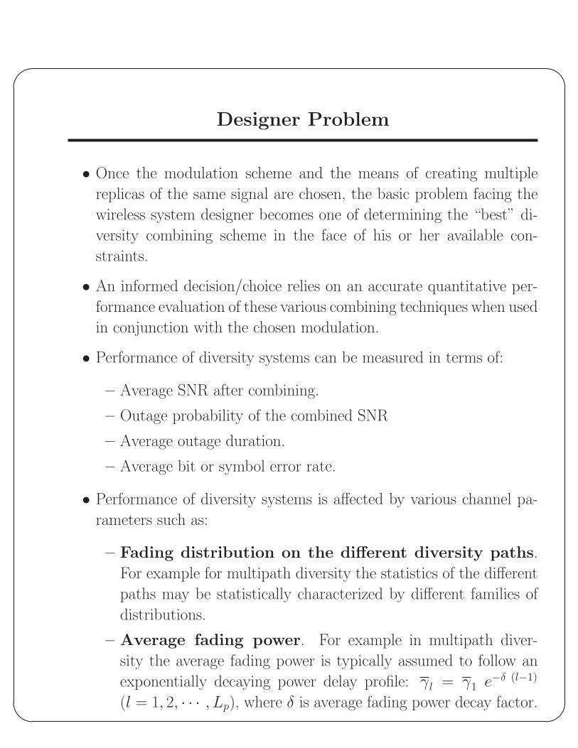
Designer Problem
• Once the modulation scheme and the means of creating multiple
replicas of the same signal are chosen, the basic problem facing the
wireless system designer becomes one of determining the “best” di-
versity combining scheme in the face of his or her available con-
straints.
• An informed decision/choice relies on an accurate quantitative per-
formance evaluation of these various combining techniques when used
in conjunction with the chosen modulation.
• Performance of diversity systems can be measured in terms of:
– Average SNR after combining.
– Outage probability of the combined SNR
– Average outage duration.
– Average bit or symbol error rate.
• Performance of diversity systems is affected by various channel pa-
rameters such as:
– Fading distribution on the different diversity paths.
For example for multipath diversity the statistics of the different
paths may be statistically characterized by different families of
distributions.
– Average fading power. For example in multipath diver-
sity the average fading power is typically assumed to follow an
exponentially decaying power delay profile: γl = γ1 e−δ (l−1)
(l = 1, 2, · · · , Lp), where δ is average fading power decay factor.
'
&
$
%
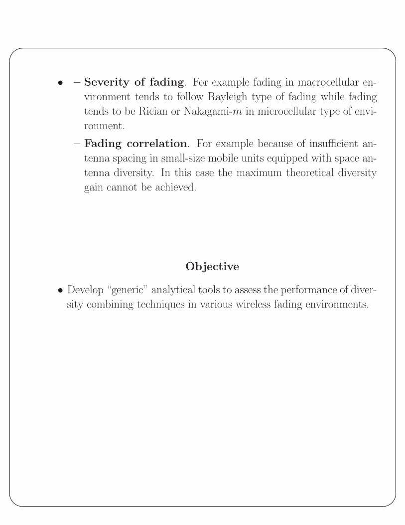
• – Severity of fading. For example fading in macrocellular en-
vironment tends to follow Rayleigh type of fading while fading
tends to be Rician or Nakagami-m in microcellular type of envi-
ronment.
– Fading correlation. For example because of insufficient an-
tenna spacing in small-size mobile units equipped with space an-
tenna diversity. In this case the maximum theoretical diversity
gain cannot be achieved.
Objective
• Develop “generic” analytical tools to assess the performance of diver-
sity combining techniques in various wireless fading environments.

'
&
$
%
Maximal-Ratio Combining (MRC)
• Let Lc denote the number of combined channels, Eb the energy-per-
bit, αl the fading amplitude of the lth channel, and Nl the noise
spectral density of the lth channel.
• For MRC the conditional (on fading amplitudes αlLcl=1) combined
SNR per bit, γt is given by
γt =
Lc∑
l=1
Eb
Nlα2
l =
Lc∑
l=1
γl.
• For binary coherent signals the conditional error probability is
Pb
(E|γlLc
l=1
)= Q
√√√√Lc∑
l=1
2gEb
Nlα2
l
= Q
√√√√2g
Lc∑
l=1
γl
,
g = 1 for BPSK, g = 1/2 for orthogonal BFSK, and g = 0.715 for
BFSK with minimum correlation.
• Average error probability is
Pb(E) =
∫ ∞
0
· · ·∫ ∞
0︸ ︷︷ ︸Lc−fold
Q
√√√√2g
Lc∑
l=1
γl
pγ1,γ2,··· ,γLc
(γ1, · · · , γLc) dγ1 · · · dγLc,
where pγ1,γ2,··· ,γLc(γ1, γ2, · · · , γLc) is the joint PDF of the γlLc
l=1.
• Two approaches to simplify this Lc-fold integral:
– Classical PDF-based approach.
– MGF-based approach which relies on the alternate representation
of the Gaussian Q-function.
'
&
$
%
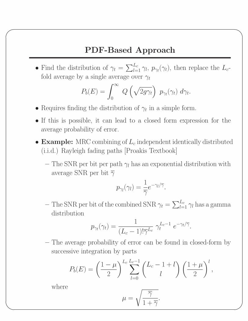
PDF-Based Approach
• Find the distribution of γt =∑Lc
l=1 γl, pγt(γt), then replace the Lc-
fold average by a single average over γt
Pb(E) =
∫ ∞
0
Q(√
2gγt
)pγt(γt) dγt.
• Requires finding the distribution of γt in a simple form.
• If this is possible, it can lead to a closed form expression for the
average probability of error.
• Example: MRC combining of Lc independent identically distributed
(i.i.d.) Rayleigh fading paths [Proakis Textbook]
– The SNR per bit per path γl has an exponential distribution with
average SNR per bit γ
pγl(γl) =
1
γe−γl/γ.
– The SNR per bit of the combined SNR γt =∑Lc
l=1 γl has a gamma
distribution
pγt(γt) =1
(Lc − 1)!γLcγLc−1
t e−γt/γ.
– The average probability of error can be found in closed-form by
successive integration by parts
Pb(E) =
(1− µ
2
)Lc Lc−1∑
l=0
(Lc − 1 + l
l
)(1 + µ
2
)l
,
where
µ =
√γ
1 + γ.

'
&
$
%
Limitations of the PDF-Based Approach
• Finding the PDF of the combined SNR per bit γt in a simple form
is typically feasible if the paths are i.i.d.
• More difficult problem if the combined paths are correlated or come
from the same family of fading distribution (e.g., Rice) but have
different parameters (e.g., different average fading powers (i.e., a
nonuniform power delay profile) and/or different severity of fading
parameters).
• Intractable in a simple form if the paths have fading distributions
coming from different families of distributions or if they have an
arbitrary correlation profile.
• We now show how the alternative representation of the Gaussian
Q-function provides a simple and elegant solution to many of these
limitations.

'
&
$
%
Alternative Form of the Gaussian Q-function
• The Gaussian Q-function is traditionally defined by
Q(x) =1√2π
∫ ∞
x
e−t2/2 dt.
– The argument x is in the lower limit of the integral.
• A preferred representation of the Gaussian Q-function is given by [Nut-
tal 72, Weinstein 74, Pawula et al. 78, and Craig 91]
Q(x) =1
π
∫ π/2
0
exp
(− x2
2 sin2 φ
)dφ; x ≥ 0.
– Finite-range integration.
– Limits are independent of the argument x.
– Integrand is exponential in the argument x.
• Additional property of alternate representation
– Integrand is maximum at φ = π/2.
– Replacing the integrand by its maximum value yields
Q(x) ≤ 1
2e−x2/2; x ≥ 0,
which is the well-known Chernoff bound.
'
&
$
%
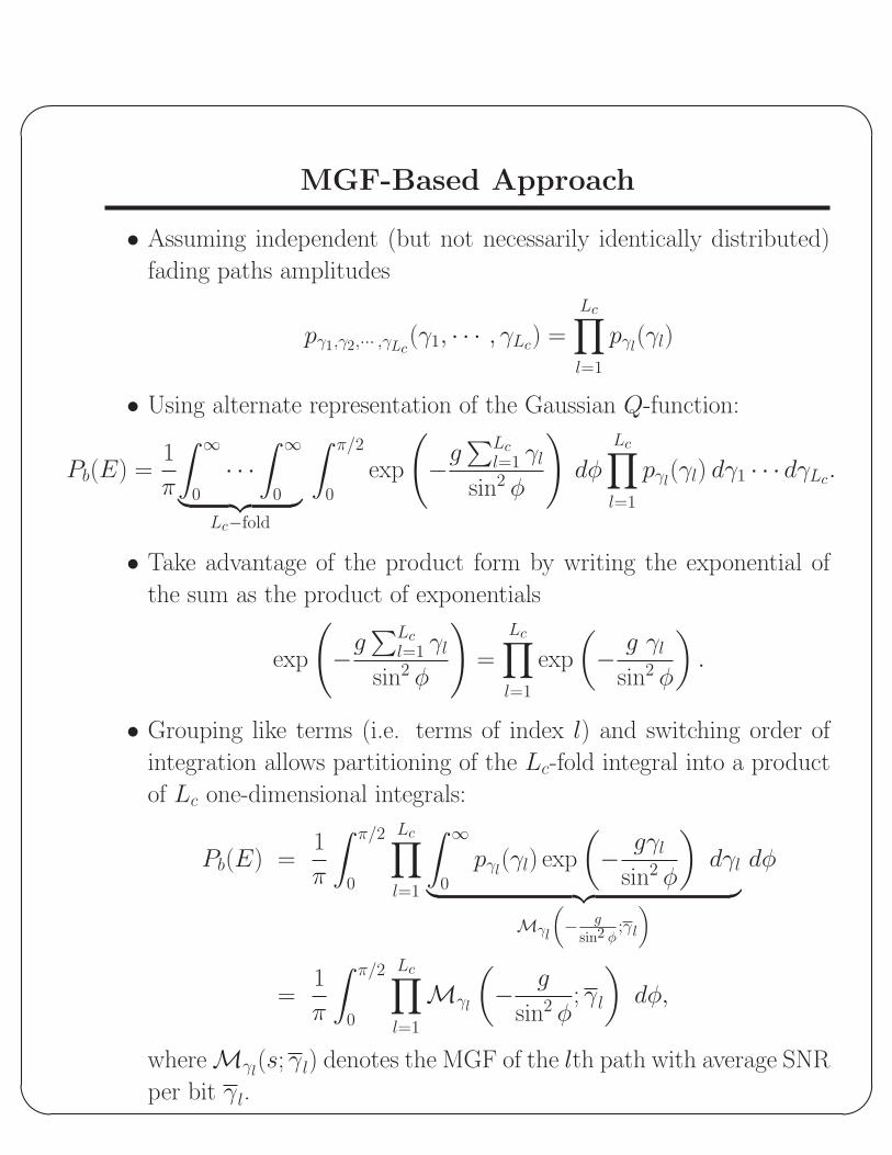
MGF-Based Approach
• Assuming independent (but not necessarily identically distributed)
fading paths amplitudes
pγ1,γ2,··· ,γLc(γ1, · · · , γLc) =
Lc∏
l=1
pγl(γl)
• Using alternate representation of the Gaussian Q-function:
Pb(E) =1
π
∫ ∞
0
· · ·∫ ∞
0︸ ︷︷ ︸Lc−fold
∫ π/2
0
exp
(−g
∑Lcl=1 γl
sin2 φ
)dφ
Lc∏
l=1
pγl(γl) dγ1 · · · dγLc.
• Take advantage of the product form by writing the exponential of
the sum as the product of exponentials
exp
(−g
∑Lcl=1 γl
sin2 φ
)=
Lc∏
l=1
exp
(− g γl
sin2 φ
).
• Grouping like terms (i.e. terms of index l) and switching order of
integration allows partitioning of the Lc-fold integral into a product
of Lc one-dimensional integrals:
Pb(E) =1
π
∫ π/2
0
Lc∏
l=1
∫ ∞
0
pγl(γl) exp
(− gγl
sin2 φ
)dγl
︸ ︷︷ ︸Mγl
(− g
sin2 φ;γl
)
dφ
=1
π
∫ π/2
0
Lc∏
l=1
Mγl
(− g
sin2 φ; γl
)dφ,
whereMγl(s; γl) denotes the MGF of the lth path with average SNR
per bit γl.

'
&
$
%
MGF-Based Approach - Examples
• Nakagami-q (Hoyt) fading
Mγl
(− g
sin2 φ; γl
)=
(1 +
2 γl
sin2 φ+
4 q2l γ2
l
(1 + q2l )
2 sin4 φ
)−1/2
.
• Nakagami-n (Rice) fading
Mγl
(− g
sin2 φ; γl
)=
(1 + n2l ) sin2 φ
(1 + n2l ) sin2 φ + γl
exp
(− n2
l γl
(1 + n2l ) sin2 φ + γl
).
• Nakagami-m fading
Mγl
(− g
sin2 φ; γl
)=
(1 +
γl
ml sin2 φ
)−ml
.
• Composite Nakagami-m/log-normal fading
Mγl
(− g
sin2 φ; µl
)' 1√
π
Np∑n=1
Hxn
(1 +
10(√
2 σl xn+µl)/10
ml sin2 φ
)−ml
,
where
– Np is the order of the Hermite polynomial, HNp(.). Setting Np
to 20 is typically sufficient for excellent accuracy.
– xn are the zeros of the Np-order Hermite polynomial.
– Hxn are the weight factors of the Np-order Hermite polynomial.

'
&
$
%
Advantages of MGF-Based Approach
• Alternate representation of the the Gaussian Q-function allows par-
titioning of the integrand so that the averaging over the fading ampli-
tudes can be done independently for each path regardless of whether
the paths are identically distributed or not.
• Desired representations of the conditional symbol error rate of M -
PSK and M -QAM allows obtaining the average symbol error rate in
a generic fashion with the MGF-based approach:
– For M -PSK the average symbol error rate is given by
Ps(E) =1
π
∫ (M−1)π/M
0
Lc∏
l=1
Mγl
(− gpsk
sin2 φ; γl
)dφ,
where gpsk = sin2(π/M).
– For M -QAM the average symbol error rate is given by
Ps(E) =4
π
(1− 1√
M
) ∫ π/2
0
Lc∏
l=1
Mγl
(− gqam
sin2 φ; γl
)dφ
− 4
π
(1− 1√
M
)2 ∫ π/4
0
Lc∏
l=1
Mγl
(− gqam
sin2 φ; γl
)dφ,
where gqam = 32(M−1).
• MGF-based approach can still provide an elegant and general solu-
tion for Nakagami-m correlated combined paths.

'
&
$
%
Switched Diversity
• Motivation
– MRC and EGC require all or some of the channel state informa-
tion (fading amplitude, phase, and delay) from all the received
signals.
– For MRC and EGC a separate receiver chain is needed for each
diversity branch, which adds to the overall receiver complexity.
– SC type systems only process one of the diversity branches but
may be not very practical in its conventional form since it still
requires the simultaneous and continuous monitoring of all the
diversity branches.
– SC often implemented in the form of switched diversity.
• Mode of Operation
– Receiver selects a particular branch until its SNR drops below a
predetermined threshold.
– When this happens the receiver switches to another branch.
– For dual branch switch and stay combining (SSC) the receiver
switches to, and stays with, the other branch regardless of whether
or not the SNR of that branch is above or below the predeter-
mined threshold.

'
&
$
%
CDF and PDF of SSC Output
• Let γssc denote the the SNR per bit at the output of the SSC combiner
and let γT denote the predetermined switching threshold.
• The CDF of SSC output is defined by
Pγssc(γ) = Prob[γssc ≤ γ]
• Assuming that the two combined branches are i.i.d. then
Pγssc(γ) =
Prob[(γ1 ≤ γT ) and (γ2 ≤ γ)], γ < γT
Prob[(γT ≤ γ1 ≤ γ) or (γ1 ≤ γT and γ2 ≤ γ)] γ ≥ γT ,
which can be expressed in terms of the CDF of the individual branches,
Pγ(γ), as
Pγssc(γ) =
Pγ(γT ) Pγ(γ) γ < γT
Pγ(γ)− Pγ(γT ) + Pγ(γ) Pγ(γT ) γ ≥ γT .
• Differentiating Pγssc(γ) with respect to γ we get the PDF of the
SSC output in terms of the CDF Pγ(γ) and the PDF pγ(γ) of the
individual branches
pγssc(γ) =dPγssc(γ)
dγ=
Pγ(γT ) pγ(γ) γ < γT
(1 + Pγ(γT )) pγ(γ) γ ≥ γT .
• For example for Nakagami-m fading
pγ(γ) =mm γm−1
γm Γ(m)exp
(−m γ
γ
); γ ≥ 0.
Pγ(γ) = 1−Γ
(m, m
γ γ)
Γ(m); γ ≥ 0.
.
'
&
$
%
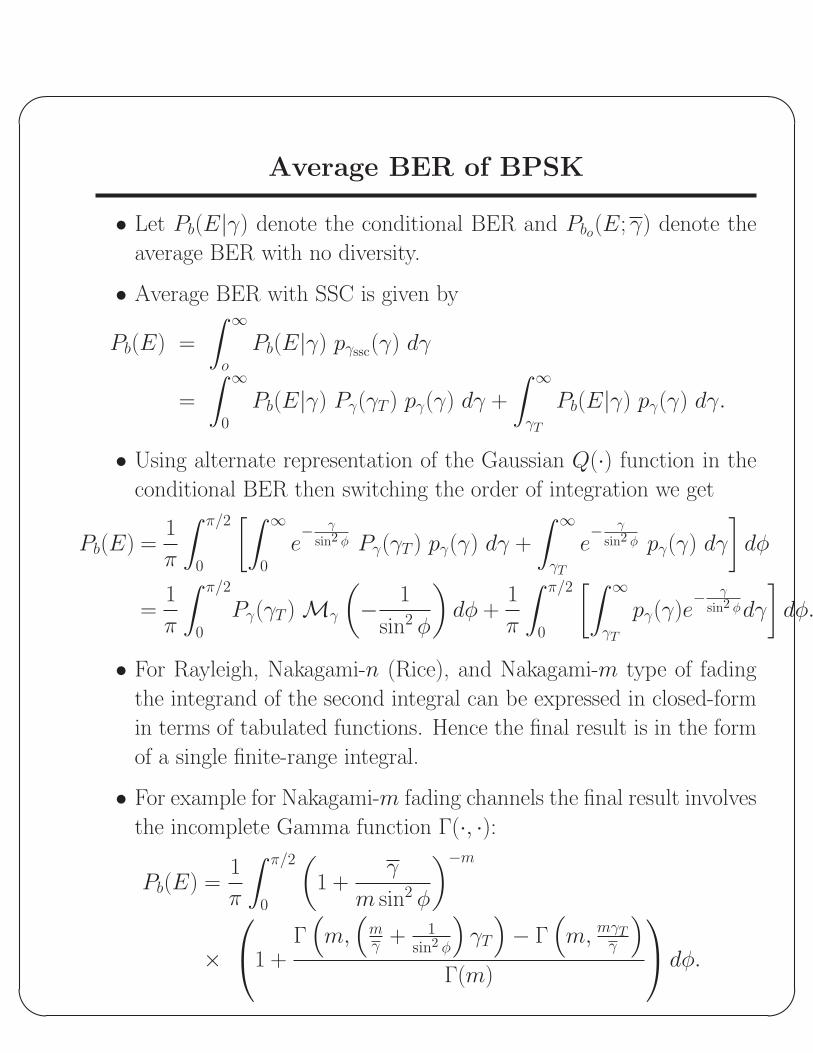
Average BER of BPSK
• Let Pb(E|γ) denote the conditional BER and Pbo(E; γ) denote the
average BER with no diversity.
• Average BER with SSC is given by
Pb(E) =
∫ ∞
o
Pb(E|γ) pγssc(γ) dγ
=
∫ ∞
0
Pb(E|γ) Pγ(γT ) pγ(γ) dγ +
∫ ∞
γT
Pb(E|γ) pγ(γ) dγ.
• Using alternate representation of the Gaussian Q(·) function in the
conditional BER then switching the order of integration we get
Pb(E) =1
π
∫ π/2
0
[∫ ∞
0
e− γ
sin2 φ Pγ(γT ) pγ(γ) dγ +
∫ ∞
γT
e− γ
sin2 φ pγ(γ) dγ
]dφ
=1
π
∫ π/2
0
Pγ(γT ) Mγ
(− 1
sin2 φ
)dφ +
1
π
∫ π/2
0
[∫ ∞
γT
pγ(γ)e− γ
sin2 φdγ
]dφ.
• For Rayleigh, Nakagami-n (Rice), and Nakagami-m type of fading
the integrand of the second integral can be expressed in closed-form
in terms of tabulated functions. Hence the final result is in the form
of a single finite-range integral.
• For example for Nakagami-m fading channels the final result involves
the incomplete Gamma function Γ(·, ·):
Pb(E) =1
π
∫ π/2
0
(1 +
γ
m sin2 φ
)−m
×1 +
Γ(m,
(mγ + 1
sin2 φ
)γT
)− Γ
(m, mγT
γ
)
Γ(m)
dφ.
'
&
$
%
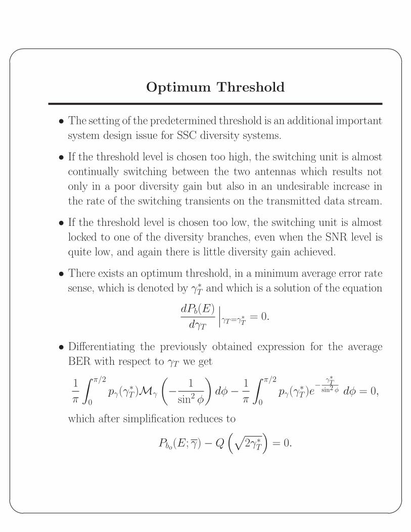
Optimum Threshold
• The setting of the predetermined threshold is an additional important
system design issue for SSC diversity systems.
• If the threshold level is chosen too high, the switching unit is almost
continually switching between the two antennas which results not
only in a poor diversity gain but also in an undesirable increase in
the rate of the switching transients on the transmitted data stream.
• If the threshold level is chosen too low, the switching unit is almost
locked to one of the diversity branches, even when the SNR level is
quite low, and again there is little diversity gain achieved.
• There exists an optimum threshold, in a minimum average error rate
sense, which is denoted by γ∗T and which is a solution of the equation
dPb(E)
dγT
∣∣∣γT =γ∗T = 0.
• Differentiating the previously obtained expression for the average
BER with respect to γT we get
1
π
∫ π/2
0
pγ(γ∗T )Mγ
(− 1
sin2 φ
)dφ− 1
π
∫ π/2
0
pγ(γ∗T )e
− γ∗Tsin2 φ dφ = 0,
which after simplification reduces to
Pbo(E; γ)−Q(√
2γ∗T)
= 0.
'
&
$
%
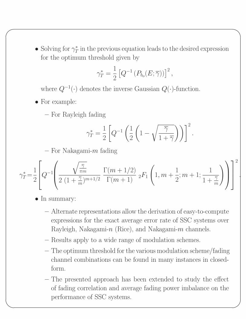
• Solving for γ∗T in the previous equation leads to the desired expression
for the optimum threshold given by
γ∗T =1
2
[Q−1 (Pbo(E; γ))
]2,
where Q−1(·) denotes the inverse Gaussian Q(·)-function.
• For example:
– For Rayleigh fading
γ∗T =1
2
[Q−1
(1
2
(1−
√γ
1 + γ
))]2
.
– For Nakagami-m fading
γ∗T =1
2
Q−1
√γ
πm
2 (1 + γm)m+1/2
Γ(m + 1/2)
Γ(m + 1)2F1
(1,m +
1
2; m + 1;
1
1 + γm
)
2
.
• In summary:
– Alternate representations allow the derivation of easy-to-compute
expressions for the exact average error rate of SSC systems over
Rayleigh, Nakagami-n (Rice), and Nakagami-m channels.
– Results apply to a wide range of modulation schemes.
– The optimum threshold for the various modulation scheme/fading
channel combinations can be found in many instances in closed-
form.
– The presented approach has been extended to study the effect
of fading correlation and average fading power imbalance on the
performance of SSC systems.
'
&
$
%
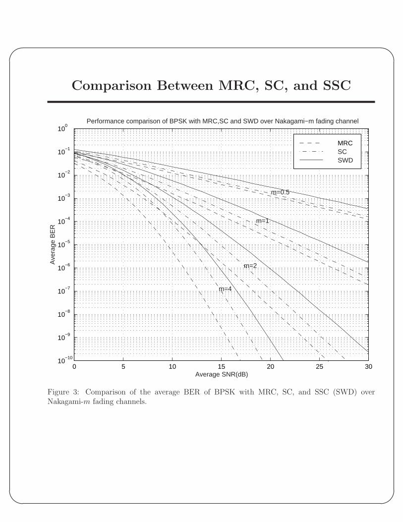
Comparison Between MRC, SC, and SSC
0 5 10 15 20 25 3010
−10
10−9
10−8
10−7
10−6
10−5
10−4
10−3
10−2
10−1
100
Ave
rage
BE
R
Average SNR(dB)
Performance comparison of BPSK with MRC,SC and SWD over Nakagami−m fading channel
m=0.5
m=1
m=2
m=4
MRCSC SWD
Figure 3: Comparison of the average BER of BPSK with MRC, SC, and SSC (SWD) overNakagami-m fading channels.

'
&
$
%
Comparison Between MRC, SC, and SSC
0 5 10 15 20 25 3010
−10
10−9
10−8
10−7
10−6
10−5
10−4
10−3
10−2
10−1
100
Average SNR (dB)
Ave
rage
SE
R
Performance Comparison of 8−PSK with MRC,SC and SWD over Nakagami−m channel
m=0.5
m=1
m=2
m=4
MRCSC SWD
Figure 4: Comparison of the average SER of 8-PSK with MRC, SC, and SSC (SWD) overNakagami-m fading channels.
'
&
$
%
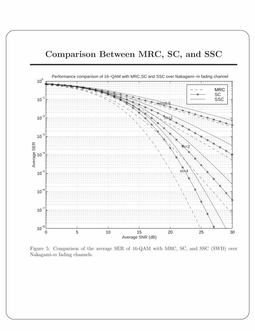
Comparison Between MRC, SC, and SSC
0 5 10 15 20 25 3010
−8
10−7
10−6
10−5
10−4
10−3
10−2
10−1
100
Average SNR (dB)
Ave
rage
SE
R
Performance comparison of 16−QAM with MRC,SC and SSC over Nakagami−m fading channel
m=0.5
m=1
m=2
m=4
MRCSCSSC
Figure 5: Comparison of the average SER of 16-QAM with MRC, SC, and SSC (SWD) overNakagami-m fading channels.
'
&
$
%
Hybrid Diversity Schemes
• Generalized diversity schemes
– SC/MRC
– SC/EGC
– SSC/MRC
– SSC/EGC
• Two dimensional diversity schemes such as space-multipath diversity
(2D-RAKE reception) or frequency-multipath diversity (Multicarrier-
RAKE reception).
– MRC/MRC
– SC/MRC

'
&
$
%
Generalized Selection Combining (GSC)
• Motivation
– Complexity of MRC and EGC receivers depends on the number
of diversity paths available which is a function of the channel
characteristics in the case of multipath diversity.
– MRC is sensitive to channel estimation errors and these errors
tend to be more important when the instantaneous SNR is low.
– Postdetection noncoherent EGC suffers from combining loss as
the number of diversity branches increases.
– SC uses only one path out of the L available multipaths and
hence does not fully exploit the amount of diversity offered by
the channel.
– GSC was introduced as a “bridge” between the two extreme com-
bining techniques offered by SC and MRC (or EGC) by combin-
ing the Lc strongest paths among the L available.
– We denote such a hybrid scheme as SC/MRC-Lc/L or SC/EGC-
Lc/L.
• Goals
– Eng, Kong and Milstein studied the average BER of SC/MRC-
2/L and SC/MRC-3/L over Rayleigh fading channels by using
a PDF-based approach which becomes “extremely unwieldy no-
tationally” for Lc ≥ 4.
– We propose to use the MGF-based approach to derive generic
expressions valid for any Lc ≤ L and for a wide variety of mod-
ulation schemes.

'
&
$
%
GSC Output Statistics
• Let γ1:L, γ2:L, · · · , γL:L denote the order statistics obtained by
arranging the γlLl=1 in decreasing order of magnitude.
• Assuming that the γlLl=1 are i.i.d. then the joint PDF of the
γl:LLcl=1 is given by [Papoulis]
pγ1:L,··· ,γLc:L(γ1:L, · · · , γLc:L)=Lc!
(L
Lc
)[Pγ(γLc:L)]L−Lc
Lc∏
l=1
pγ(γl:L),
with
γ1:L ≥ · · · ≥ γLc:L ≥ 0,
pγ(γ) =1
γe−
γγ ,
Pγ(γ) = 1− e−γγ .
• It is important to note that although the γlLl=1 are independent
the γl:LLl=1 are not.
• The MGF-based approach relies on finding a simple expression for
Mγt(s)=Eγt[esγt] = Eγ1:L,γ2:L,··· ,γLc:L
[es
∑Lcl=1 γl:L
]
=
∫ ∞
0
∫ ∞
γLc:L
· · ·∫ ∞
γ2:L︸ ︷︷ ︸Lc−fold
pγ1:L,··· ,γLc:L(γ1:L, · · · , γLc:L)es
∑Lcl=1 γl:Ldγ1:L · · · dγLc:L.
• Problem: Although the integrand is in a desirable separable form
in the γl:Lc’s, we cannot partition the Lc-fold integral into a product
of one-dimensional integrals as was possible for MRC because of the
γl:L’s in the lower limits of the semi-finite range (improper) integrals.

'
&
$
%
A Useful Theorem
• Theorem [Sukhatme 1937]: Defining the “spacing”
xl4= γl:L − γl+1:L (l = 1, 2, · · · , L− 1)
xL4= γL:L
then the xlLl=1 are
– Independently distributed
– Distributed according to an exponential distribution
pxl(xl) =
l
γe−
lxlγ , xl ≥ 0, (l = 1, 2, · · · , L)
• Sketch of the Proof:
– Since the Jacobian of the transformation is equal to 1 we have
px1,··· ,xL(x1, · · · , xL) = pγ1:L,··· ,γL:L(γ1:L, · · · , γL:L)
=L!
γLexp
(−
∑Ll=1 γl:L
γ
).
– The γl:L’s can be expressed in terms of the xl’s as
γl:L =
L∑
k=l
xk.
– Hence
px1,··· ,xL(x1, · · · , xL) =
L!
γLexp
(−x1 + 2x2 + · · · + LxL
γ
)
=
L∏
l=1
l
γexp
(−lxl
γ
). QED

'
&
$
%
MGF of GSC Combined SNR
• We use the previous theorem to derive a simple expression for the
MGF of the combined SNR γt given by
γt =
Lc∑
l=1
γl:L =
Lc∑
l=1
L∑
k=l
xk
= x1 + 2x2 + · · · + LcxLc + LcxLc+1 + · · · + LcxL.
1. Rewriting the MGF of γt in terms of the xl’s as
Mγt(s)=
∫ ∞
0
· · ·∫ ∞
0︸ ︷︷ ︸L−fold
px1,··· ,xL(x1,· · · ,xL)es(x1+2x2+···+LcxLc+LcxLc+1+···+LcxL)dx1· · ·dxL.
2. Since the xl’s are independent px1,··· ,xL(x1, · · · , xL) =
∏Ll=1 pxl
(xl)
and we can hence put the integrand in a product form
Mγt(s)=
∫ ∞
0
· · ·∫ ∞
0︸ ︷︷ ︸L−fold
[L∏
l=1
pxl(xl)
]esx1e2sx2 · · · eLcsxLceLcsxLc+1 · · · eLcsxLdx1· · ·dxL.
3. Grouping like terms and partitioning the L-fold integral into a
product of L one-dimensional integrals
Mγt(s)=
[∫ ∞
0
esx1px1(x1)dx1
][∫ ∞
0
e2sx2px2(x2)dx2
]· · ·
[∫ ∞
0
eLcsxLcpxLc(xLc)dxLc
]
×[∫ ∞
0
eLcsxLc+1pxLc+1(xLc+1)dxLc+1
]· · ·
[∫ ∞
0
eLcsxLpxL(xL)dxL
].
4. Using the fact that the xl’s are exponentially distributed we get
the final desired closed-form result as
Mγt(s) = (1− sγ)−Lc
L∏
l=Lc+1
(1− sγLc
l
)−1
.
'
&
$
%
Average Combined SNR of GSC
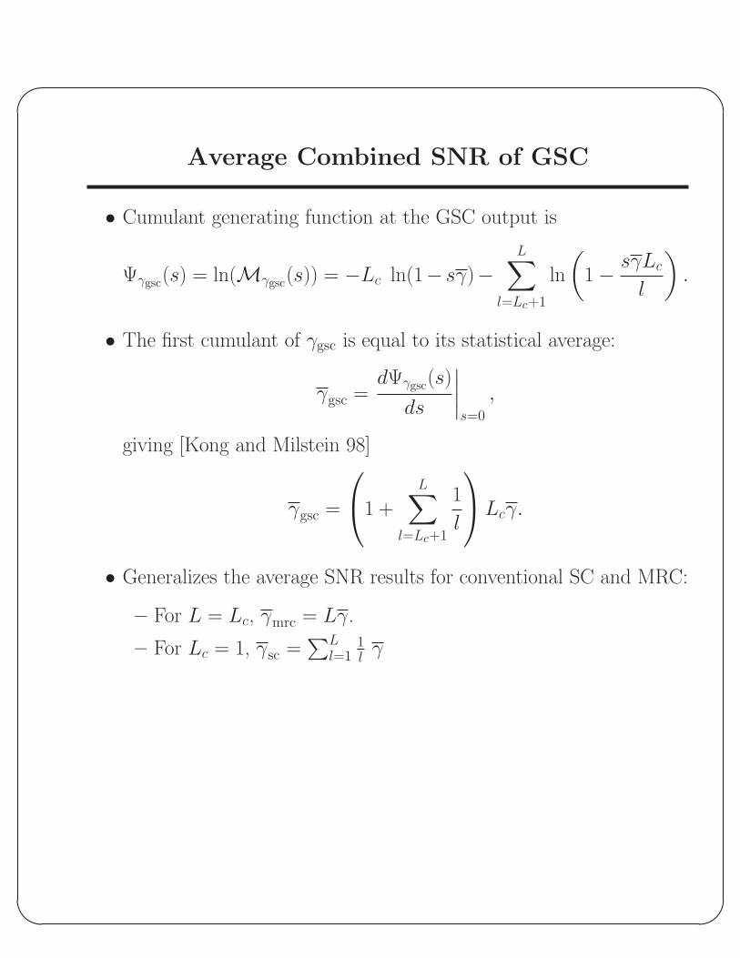
• Cumulant generating function at the GSC output is
Ψγgsc(s) = ln(Mγgsc(s)) = −Lc ln(1− sγ)−L∑
l=Lc+1
ln
(1− sγLc
l
).
• The first cumulant of γgsc is equal to its statistical average:
γgsc =dΨγgsc(s)
ds
∣∣∣∣s=0
,
giving [Kong and Milstein 98]
γgsc =
1 +
L∑
l=Lc+1
1
l
Lcγ.
• Generalizes the average SNR results for conventional SC and MRC:
– For L = Lc, γmrc = Lγ.
– For Lc = 1, γsc =∑L
l=11l γ
'
&
$
%
Average Combined SNR of GSC
0 5 10 15 20 25 300
5
10
15
20
25
30
35Average combined SNR (L=3)
Average SNR per symbol per path [dB]
Ave
rage
com
bine
d S
NR
per
sym
bol [
dB]
(a) Lc=1
(c) Lc=3
0 5 10 15 20 25 300
5
10
15
20
25
30
35Average combined SNR (L=4)
Average SNR per symbol per path [dB]
Ave
rage
com
bine
d S
NR
per
sym
bol [
dB]
(a) Lc=1
(d) Lc=4
0 5 10 15 20 25 300
5
10
15
20
25
30
35Average combined SNR (L=5)
Average SNR per symbol per path [dB]
Ave
rage
com
bine
d S
NR
per
sym
bol [
dB]
(a) Lc=1
(e) Lc=5
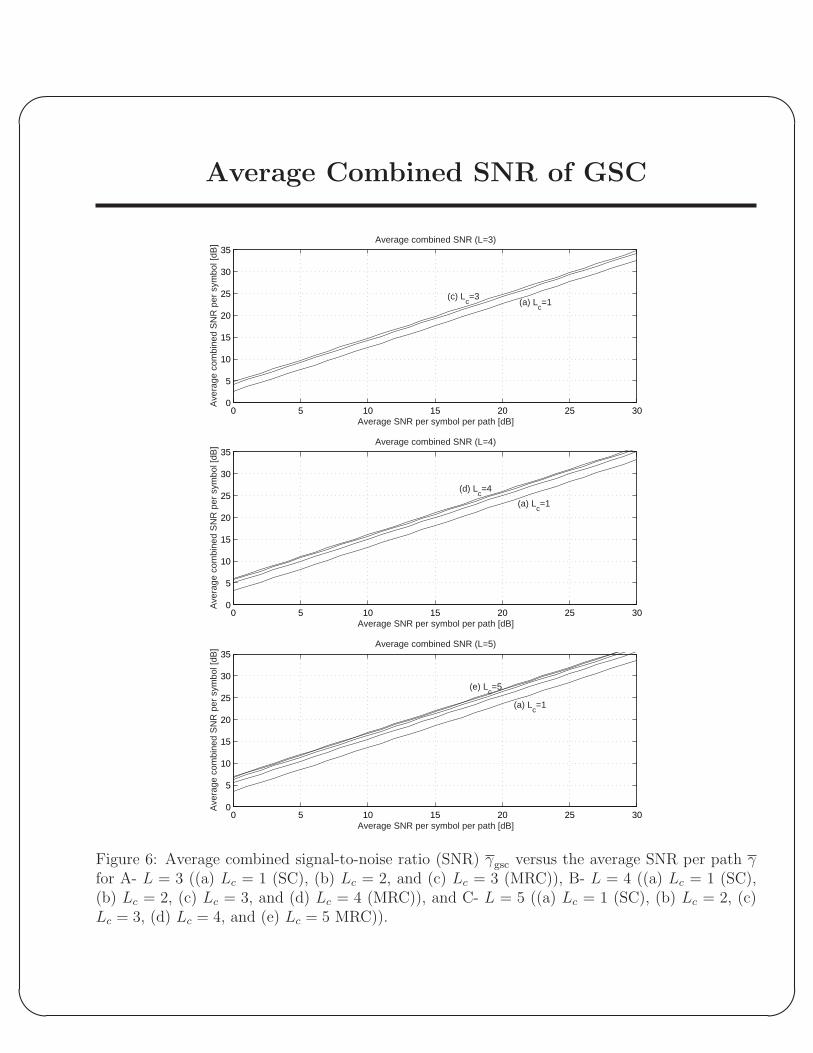
Figure 6: Average combined signal-to-noise ratio (SNR) γgsc versus the average SNR per path γfor A- L = 3 ((a) Lc = 1 (SC), (b) Lc = 2, and (c) Lc = 3 (MRC)), B- L = 4 ((a) Lc = 1 (SC),(b) Lc = 2, (c) Lc = 3, and (d) Lc = 4 (MRC)), and C- L = 5 ((a) Lc = 1 (SC), (b) Lc = 2, (c)Lc = 3, (d) Lc = 4, and (e) Lc = 5 MRC)).

'
&
$
%
Average Combined SNR of GSC
0 5 10 15 20 25 300
5
10
15
20
25
30
35
Average combined SNR (Lc=3)
Average SNR per symbol per path [dB]
Ave
rage
com
bine
d S
NR
per
sym
bol [
dB] (a) L=3
(c) L=5
Figure 7: Average combined signal-to-noise ratio (SNR) γgsc versus the average SNR per path γfor Lc = 3 ((a) L = 3, (b) L = 4, and (c) L = 5.

'
&
$
%
Performance of 16-QAM with GSC
0 5 10 15 20 25 3010
−8
10−6
10−4
10−2
100
Average Symbol Error Rate of 16−QAM (L=3)
Average SNR per symbol per path [dB]
Ave
rage
Sym
bol E
rror
Rat
e P
s(E)
(a) Lc=1
(c) Lc=3
0 5 10 15 20 25 3010
−10
10−8
10−6
10−4
10−2
100
Average Symbol Error Rate of 16−QAM (L=4)
Average SNR per symbol per path [dB]
Ave
rage
Sym
bol E
rror
Rat
e P
s(E)
(a) Lc=1
(d) Lc=4
0 5 10 15 20 25 3010
−10
10−8
10−6
10−4
10−2
100
Average Symbol Error Rate of 16−QAM (L=5)
Average SNR per symbol per path [dB]
Ave
rage
Sym
bol E
rror
Rat
e P
s(E)
(a) Lc=1
(e) Lc=5
Figure 8: Average symbol error rate (SER) Ps(E) of 16-QAM versus the average SNR per symbolper path γ for A- L = 3 ((a) Lc = 1 (SC), (b) Lc = 2, and (c) Lc = 3 (MRC)), B- L = 4 ((a)Lc = 1 (SC), (b) Lc = 2, (c) Lc = 3, and (d) Lc = 4 (MRC)), and C- L = 5 ((a) Lc = 1 (SC), (b)Lc = 2, (c) Lc = 3, (d) Lc = 4, and (e) Lc = 5 MRC)).
'
&
$
%
Performance of 16-QAM with GSC
0 5 10 15 20 25 3010
−10
10−9
10−8
10−7
10−6
10−5
10−4
10−3
10−2
10−1
100
Average Symbol Error Rate of 16−QAM (Lc=3)
Average SNR per symbol per path [dB]
Ave
rage
Sym
bol E
rror
Rat
e P
s(E)
(a) L=3
(b) L=4
(c) L=5
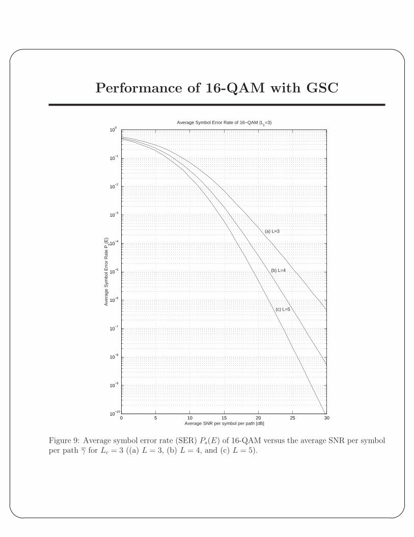
Figure 9: Average symbol error rate (SER) Ps(E) of 16-QAM versus the average SNR per symbolper path γ for Lc = 3 ((a) L = 3, (b) L = 4, and (c) L = 5).

'
&
$
%
Impact of Correlation on the Performanceof MRC Diversity Systems
• Motivation
– In some real life scenarios the independence assumption is not
valid (e.g. insufficient antenna spacing in small-size mobile units
equipped with space antenna diversity).
– In correlated fading conditions the maximum theoretical diversity
gain cannot be achieved.
– Effect of correlation between the combined signals has to be taken
into account for the accurate performance analysis of diversity
systems.
• Goal
– Obtain generic easy-to-compute formulas for the exact average
error probability in correlated fading environment:
∗ Accounting for the average SNR imbalance and severity of
fading (Nakagami-m).
∗ A variety of correlation models.
∗ Wide range of modulation schemes.
• Tools
– The unified moment generating function (MGF) based approach.
– Mathematical studies on the multivariate gamma distribution
(Krishnamoorthy and Parthasarathy 51, Gurland 55, and Kotz
and Adams 64).
'
&
$
%
Summary of the MGF-based Approach
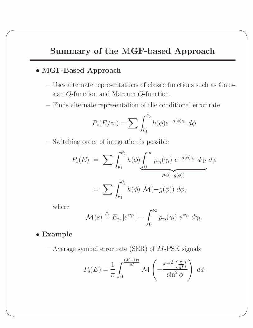
• MGF-Based Approach
– Uses alternate representations of classic functions such as Gaus-
sian Q-function and Marcum Q-function.
– Finds alternate representation of the conditional error rate
Ps(E/γt) =∑ ∫ θ2
θ1
h(φ)e−g(φ)γt dφ
– Switching order of integration is possible
Ps(E) =∑ ∫ θ2
θ1
h(φ)
∫ ∞
0
pγt(γt) e−g(φ)γt dγt
︸ ︷︷ ︸M(−g(φ))
dφ
=∑ ∫ θ2
θ1
h(φ) M(−g(φ)) dφ,
where
M(s)4= Eγt [esγt] =
∫ ∞
0
pγt(γt) esγt dγt.
• Example
– Average symbol error rate (SER) of M -PSK signals
Ps(E) =1
π
∫ (M−1)πM
0
M(−sin2
(πM
)
sin2 φ
)dφ

'
&
$
%
Model A: Dual Diversity
• Two correlated branches with nonidentical fading (e.g. polarization
diversity).
• PDF of the combined SNR
pa(γt) =
√π
Γ(m)
[m2
γ1γ2(1− ρ)
]m (γt
2β′
)m−12
Im−12(β′γt) e−α′γt; γt ≥ 0,
where
ρ =cov(r2
1, r22)√
var(r21)var(r2
2), 0 ≤ ρ < 1.
is the envelope correlation coefficient between the two signals, and
α′4=
α
Es/N0=
m(γ1 + γ2)
2γ1γ2(1− ρ),
β′4=
β
Es/N0=
m((γ1 + γ2)
2 − 4γ1γ2(1− ρ))1/2
2γ1γ2(1− ρ).
• MGF of the combined SNR per symbol
Ma(s) =
(1− (γ1 + γ2)
ms +
(1− ρ)γ1γ2
m2s2
)−m
; s ≥ 0.
• With this model for BPSK the MGF-based approach gives an alter-
nate form to the previous equivalent result [Aalo 95] which required
the evaluation of the Appell’s hypergeometric function, F2(·; ·, ·; ·, ·; ·, ·).
'
&
$
%
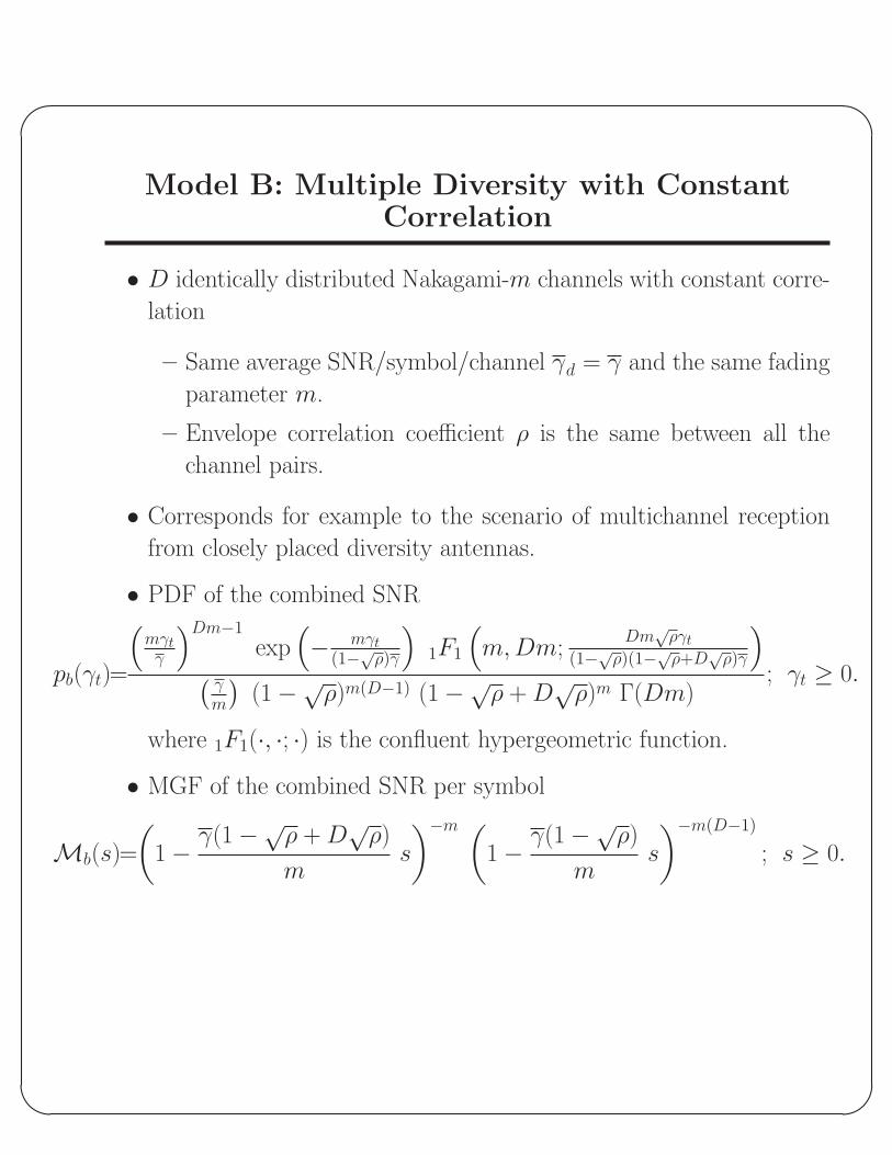
Model B: Multiple Diversity with ConstantCorrelation
• D identically distributed Nakagami-m channels with constant corre-
lation
– Same average SNR/symbol/channel γd = γ and the same fading
parameter m.
– Envelope correlation coefficient ρ is the same between all the
channel pairs.
• Corresponds for example to the scenario of multichannel reception
from closely placed diversity antennas.
• PDF of the combined SNR
pb(γt)=
(mγtγ
)Dm−1
exp(− mγt
(1−√ρ)γ
)1F1
(m,Dm;
Dm√
ργt
(1−√ρ)(1−√ρ+D√
ρ)γ
)(
γm
)(1−√ρ)m(D−1) (1−√ρ + D
√ρ)m Γ(Dm)
; γt ≥ 0.
where 1F1(·, ·; ·) is the confluent hypergeometric function.
• MGF of the combined SNR per symbol
Mb(s)=
(1− γ(1−√ρ + D
√ρ)
ms
)−m (1− γ(1−√ρ)
ms
)−m(D−1)
; s ≥ 0.

'
&
$
%
Model C: Multiple Diversity with ArbitraryCorrelation
• D identically distributed Nakagami-m channels with arbitrary cor-
relation.
– Same average SNR/symbol/channel γd = γ and the same fading
parameter m.
– Envelope correlation coefficient ρdd′ may be different between the
channel pairs.
• Useful for example to the scenario of multichannel reception from
diversity antennas in which the correlation between the pairs of com-
bined signals decays as the spacing between the antennas increases.
• PDF of the combined SNR not available in a simple form.
• MGF of the combined SNR per symbol can be deduced from the
work of [Krishnamoorthy and Parthasarathy 51]
Mc(s) = Eγ1,γ2,··· ,γD
[exp
(s
D∑
d=1
γd
)]
=
(−sγ
m
)−mD
∣∣∣∣∣∣∣∣∣∣∣∣∣
1− msγ
√ρ12 · · · √
ρ1D√ρ12 1− m
sγ · · · √ρ2D
· · · ·· · · ·· · · ·√ρ1D
√ρ2D · · · 1− m
sγ
∣∣∣∣∣∣∣∣∣∣∣∣∣
−m
D×D
,
where |[M ]|D×D denotes the determinant of the D ×D matrix M .

'
&
$
%
Special Cases of Model C
• Dual Correlation Model (Model A)
– A dual correlation model (D = 2) has a correlation matrix with
the following structure
M =
[1− m
sγ
√ρ√
ρ 1− msγ
].
– Application: Small size terminals equipped with space diversity
where antenna spacing is insufficient to provide independent fad-
ing among signal paths.
– The determinant of M can be easily found to be given by
detM =
(1− m
sγ
)2
− ρ.
– Substituting the determinant of M in the MGF we get
Mc(s)=Ma(s) =
(1− 2γ
ms +
(1− ρ)γ2
m2s2
)−m
.

'
&
$
%
• Intraclass Correlation Model (Model B)
– A correlation matrix M is called a Dth order intraclass correla-
tion matrix iff it has the following structure
M =
a b · · · b
b a b · · b
b b a b · b
· · · · · ·b · · · b a
D×D
with b ≥ − aD−1.
– Application: Very closely spaced antennas or 3 antennas placed
on an equilateral triangle.
– Theorem: If M is a Dth order intraclass correlation matrix then
detM = (a− b)D−1 (a + b(D − 1))
– For a = 1 − msγ and b =
√ρ, applying the previous theorem we
get
Mc(s)=Mb(s)=
(1− γ(1−√ρ + D
√ρ)
ms
)−m(1− γ(1−√ρ)
ms
)−m(D−1)
.
'
&
$
%
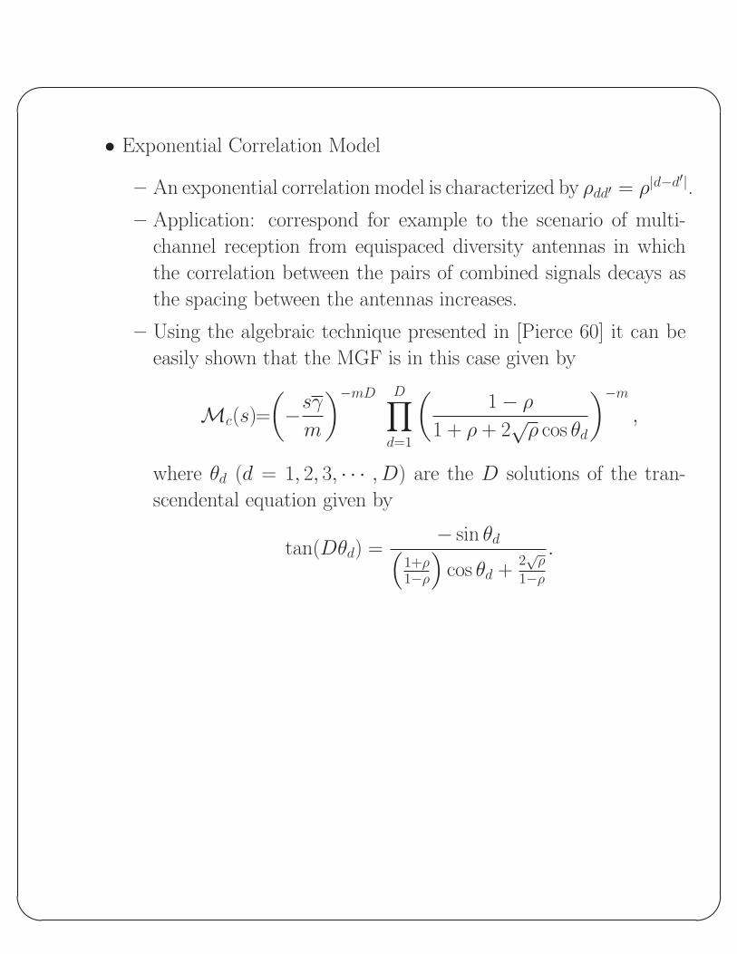
• Exponential Correlation Model
– An exponential correlation model is characterized by ρdd′ = ρ|d−d′|.
– Application: correspond for example to the scenario of multi-
channel reception from equispaced diversity antennas in which
the correlation between the pairs of combined signals decays as
the spacing between the antennas increases.
– Using the algebraic technique presented in [Pierce 60] it can be
easily shown that the MGF is in this case given by
Mc(s)=
(−sγ
m
)−mD D∏
d=1
(1− ρ
1 + ρ + 2√
ρ cos θd
)−m
,
where θd (d = 1, 2, 3, · · · , D) are the D solutions of the tran-
scendental equation given by
tan(Dθd) =− sin θd(
1+ρ1−ρ
)cos θd +
2√
ρ
1−ρ
.
'
&
$
%
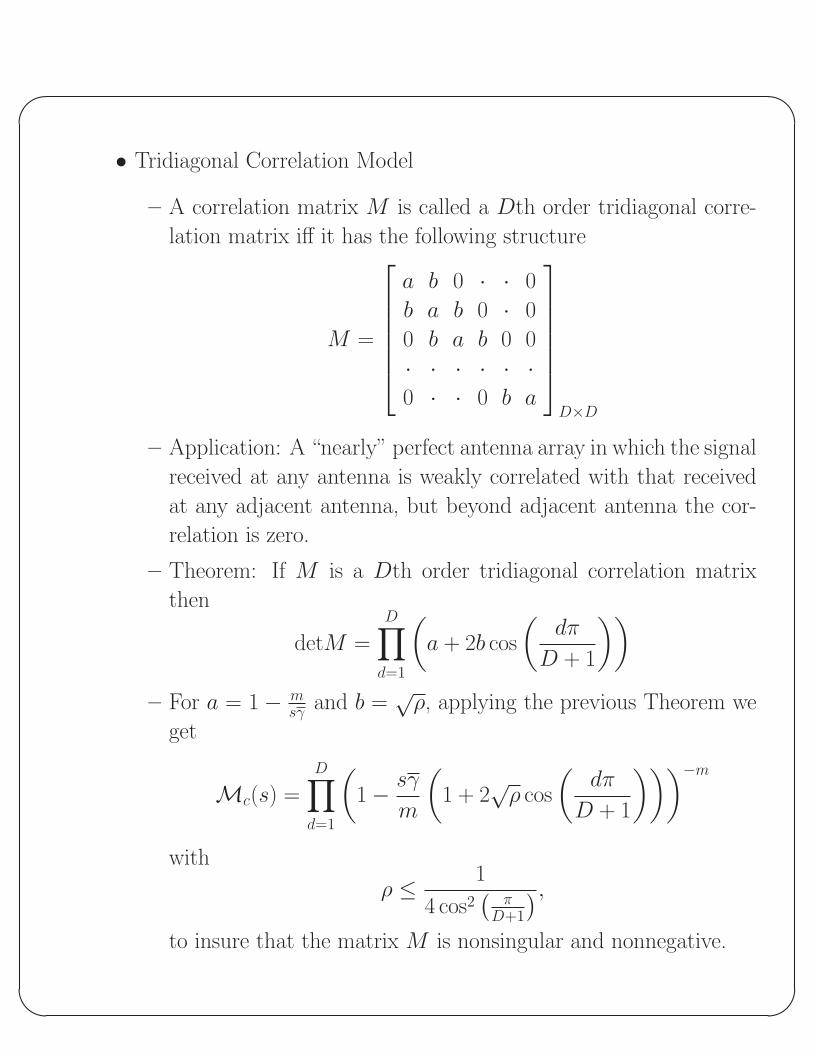
• Tridiagonal Correlation Model
– A correlation matrix M is called a Dth order tridiagonal corre-
lation matrix iff it has the following structure
M =
a b 0 · · 0
b a b 0 · 0
0 b a b 0 0
· · · · · ·0 · · 0 b a
D×D
– Application: A “nearly” perfect antenna array in which the signal
received at any antenna is weakly correlated with that received
at any adjacent antenna, but beyond adjacent antenna the cor-
relation is zero.
– Theorem: If M is a Dth order tridiagonal correlation matrix
then
detM =
D∏
d=1
(a + 2b cos
(dπ
D + 1
))
– For a = 1− msγ and b =
√ρ, applying the previous Theorem we
get
Mc(s) =
D∏
d=1
(1− sγ
m
(1 + 2
√ρ cos
(dπ
D + 1
)))−m
with
ρ ≤ 1
4 cos2(
πD+1
),
to insure that the matrix M is nonsingular and nonnegative.
'
&
$
%
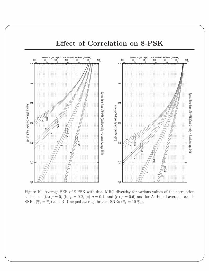
Effect of Correlation on 8-PSK
05
1015
2025
3010 −6
10 −5
10 −4
10 −3
10 −2
10 −1
10 0Symbol Error Rate of 8−PSK (Dual Diversity − Equal Average SNR)
Average SNR per Symbol per Path [dB]
Average Symbol Error Rate (SER)
m=0.5
m=1
m=2
m=4
a
a
a
a
d
d
d
d
05
1015
2025
3010 −6
10 −5
10 −4
10 −3
10 −2
10 −1
10 0Symbol Error Rate of 8−PSK (Dual Diversity − Unequal Average SNR)
Average SNR per Symbol of First Path [dB]
Average Symbol Error Rate (SER)
m=4
m=2
m=1
m=0.5
a
a
a
a
d
d
d
d
Figure 10: Average SER of 8-PSK with dual MRC diversity for various values of the correlationcoefficient ((a) ρ = 0, (b) ρ = 0.2, (c) ρ = 0.4, and (d) ρ = 0.6) and for A- Equal average branchSNRs (γ1 = γ2) and B- Unequal average branch SNRs (γ1 = 10 γ2).

'
&
$
%
Effect of Correlation on 8-PSK
05
1015
2025
3010 −6
10 −5
10 −4
10 −3
10 −2
10 −1
10 0Comparison Between Constant and Exponential Correlation (m=0.5)
Average SNR per Symbol per Path [dB]
Average Symbol Error Rate (SER) Ps(E)
D=3
D=5
a
a
d
d
Constant CorrelationExponential Correlation
05
1015
2025
3010 −6
10 −5
10 −4
10 −3
10 −2
10 −1
10 0Comparison Between Constant and Exponential Correlation (m=1)
Average SNR per Symbol per Path [dB]
Average Symbol Error Rate (SER) Ps(E)
D=3
D=5
a
a
dd
Constant CorrelationExponential Correlation
05
1015
2025
3010 −6
10 −5
10 −4
10 −3
10 −2
10 −1
10 0Comparison Between Constant and Exponential Correlation (m=2)
Average SNR per Symbol per Path [dB]
Average Symbol Error Rate (SER) Ps(E)
D=3
D=5
aad
d
Constant CorrelationExponential Correlation
05
1015
2025
3010 −6
10 −5
10 −4
10 −3
10 −2
10 −1
10 0Comparison Between Constant and Exponential Correlation (m=4)
Average SNR per Symbol per Path [dB]
Average Symbol Error Rate (SER) Ps(E)
D=3
D=5
a
add
Constant CorrelationExponential Correlation
Figure 11: Comparison of the average SER of 8-PSK with MRC diversity for constant and ex-ponential fading correlation profiles, various values of the correlation coefficient ((a) ρ = 0, (b)ρ = 0.2, (c) ρ = 0.4, and (d) ρ = 0.6), and γd = γ for d = 1, 2, · · · , D.

'
&
$
%
2D-MRC/MRC Diversity overCorrelated Fading
• We consider a two-dimensional diversity system consisting for exam-
ple of D antennas each one followed by an Lc finger RAKE receiver.
• For practical channel conditions of interest we have
– For a fixed antenna index d assume that the γl,dLcl=1’s are inde-
pendent but nonidentically distributed.
– For a fixed multipath index l assume that the γl,dDd=1’s are
correlated according to model A, B, or C (as described earlier).
• When MRC combining is done for both space and multipath diversity
we have a conditional combined SNR/bit given by
γt =
D∑
d=1
Lc∑
l=1
γl,d
=
D∑
d=1
γd (where γd =
Lc∑
l=1
γl,d)
=
Lc∑
l=1
γl (where γl =
D∑
d=1
γl,d).
• Finding the average error rate performance of such systems with the
classical PDF-based approach is difficult since the PDF of γt cannot
be found in a simple form.
• We propose to use the MGF-based approach to obtain generic results
for a wide variety of modulation schemes.
'
&
$
%
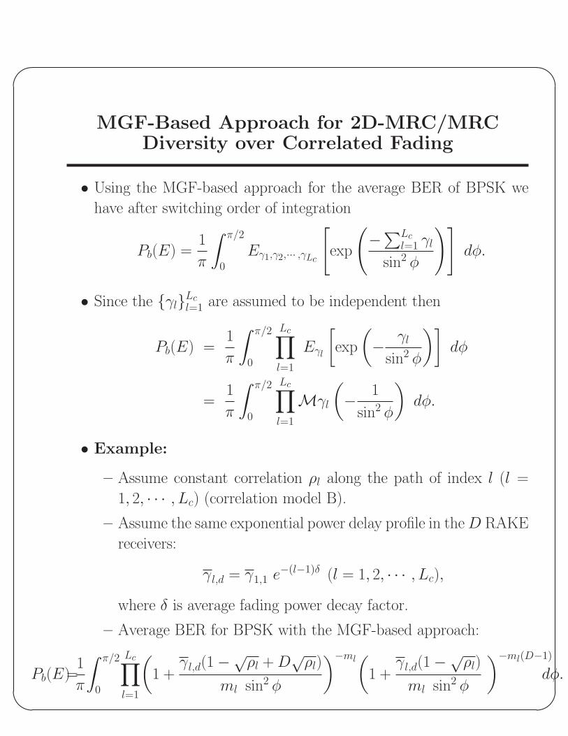
MGF-Based Approach for 2D-MRC/MRCDiversity over Correlated Fading
• Using the MGF-based approach for the average BER of BPSK we
have after switching order of integration
Pb(E) =1
π
∫ π/2
0
Eγ1,γ2,··· ,γLc
[exp
(−∑Lc
l=1 γl
sin2 φ
)]dφ.
• Since the γlLcl=1 are assumed to be independent then
Pb(E) =1
π
∫ π/2
0
Lc∏
l=1
Eγl
[exp
(− γl
sin2 φ
)]dφ
=1
π
∫ π/2
0
Lc∏
l=1
Mγl
(− 1
sin2 φ
)dφ.
• Example:
– Assume constant correlation ρl along the path of index l (l =
1, 2, · · · , Lc) (correlation model B).
– Assume the same exponential power delay profile in the D RAKE
receivers:
γl,d = γ1,1 e−(l−1)δ (l = 1, 2, · · · , Lc),
where δ is average fading power decay factor.
– Average BER for BPSK with the MGF-based approach:
Pb(E)=1
π
∫ π/2
0
Lc∏
l=1
(1 +
γl,d(1−√
ρl + D√
ρl)
ml sin2 φ
)−ml(
1 +γl,d(1−
√ρl)
ml sin2 φ
)−ml(D−1)
dφ.
'
&
$
%
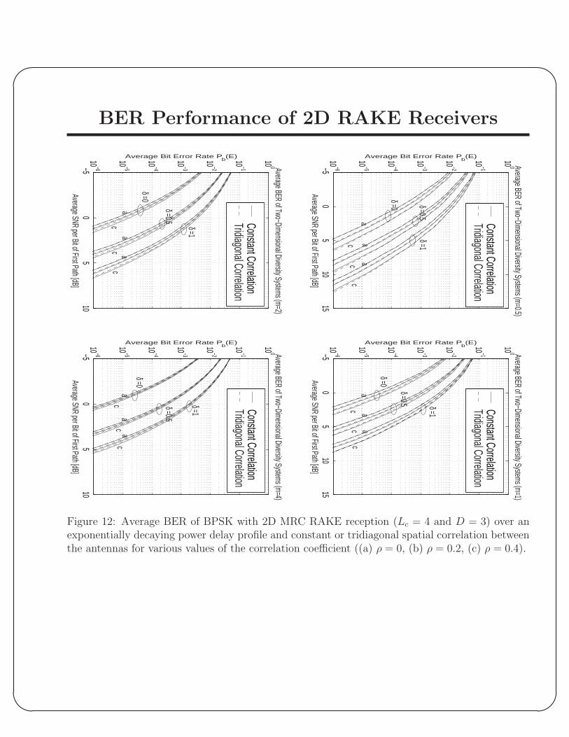
BER Performance of 2D RAKE Receivers
−50
510
1510 −6
10 −5
10 −4
10 −3
10 −2
10 −1
10 0 Average BER of Two−Dimensional Diversity Systems (m=0.5)
Average SNR per Bit of First Path [dB]
Average Bit Error Rate Pb(E)
aa
a
cc
c
δ =0 δ =0.5δ =1
Constant CorrelationTridiagonal Correlation
−50
510
1510 −6
10 −5
10 −4
10 −3
10 −2
10 −1
10 0 Average BER of Two−Dimensional Diversity Systems (m=1)
Average SNR per Bit of First Path [dB]
Average Bit Error Rate Pb(E)
aa
ac
cc
δ =1
δ =0.5
δ =0
Constant CorrelationTridiagonal Correlation
−50
510
10 −6
10 −5
10 −4
10 −3
10 −2
10 −1
10 0 Average BER of Two−Dimensional Diversity Systems (m=2)
Average SNR per Bit of First Path [dB]
Average Bit Error Rate Pb(E)
aa
ac
cc
δ =1
δ =0.5
δ =0
Constant CorrelationTridiagonal Correlation
−50
510
10 −6
10 −5
10 −4
10 −3
10 −2
10 −1
10 0 Average BER of Two−Dimensional Diversity Systems (m=4)
Average SNR per Bit of First Path [dB]
Average Bit Error Rate Pb(E)
aa
ac
cc
δ =1
δ =0.5
δ =0
Constant CorrelationTridiagonal Correlation
Figure 12: Average BER of BPSK with 2D MRC RAKE reception (Lc = 4 and D = 3) over anexponentially decaying power delay profile and constant or tridiagonal spatial correlation betweenthe antennas for various values of the correlation coefficient ((a) ρ = 0, (b) ρ = 0.2, (c) ρ = 0.4).
'
&
$
%
Optimal Transmitter Diversity
• Approximated BER of M -QAM and M -PSK
Pb(E|γ) = a · exp(−bγ).
For example, a = 0.0852 and b=0.4030 for16-QAM.
• Average BER with MRC combining
– Average BER
Pb(E) = aL∏
l=1
(1 +
bγl
ml
)−ml
,
where γl = ΩlE(l)s
Nl= ΩlPlTs
Nl= PlGl.
– Goal: Find the set PlLl=1 which minimizes the av-
erage BER subject to the total power constraint Pt =∑Ll=1 Pl.
– There exists a unique optimal power allocationsolution
∗ The constraint forms a convex set.
∗ aPb(E) is concave.

'
&
$
%
Optimal Solution
• Optimum power for minimum average BER
Pl = ml Max
[Pt∑L
k=1 mk
+
∑Lk=1
mkGk
b∑L
k=1 mk
− 1
bGl, 0
].
• For all equal Nakagami parameter m
Pl = Max
[Pt
L+
m
Lb
L∑
k=1
1
Gk− m
bGl, 0
].
• For the Rayleigh fading channel (i.e., m = 1)
Pl = Max
[Pt
L+
1
Lb
L∑
k=1
1
Gk− 1
bGl, 0
].
• Minimum average BER for 16-QAM
Pb(E) =3
4π
∫ π2
0
L∏
l=1
(1 +
2PlGl
5ml sin2 φ
)−ml
dφ
+1
4π
∫ π2
0
L∏
l=1
(1 +
18PlGl
5ml sin2 φ
)−ml
dφ.
'
&
$
%
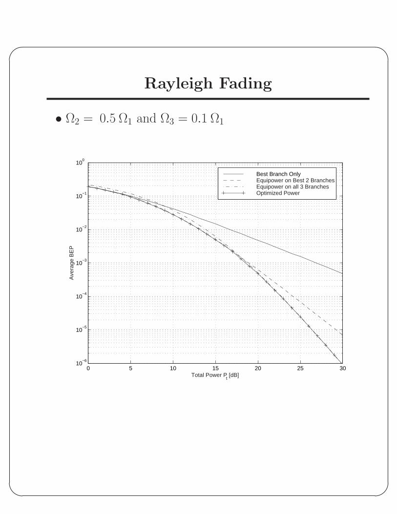
Rayleigh Fading
• Ω2 = 0.5 Ω1 and Ω3 = 0.1 Ω1
0 5 10 15 20 25 3010
−6
10−5
10−4
10−3
10−2
10−1
100
Total Power Pt [dB]
Ave
rage
BE
P
Best Branch Only Equipower on Best 2 BranchesEquipower on all 3 Branches Optimized Power

'
&
$
%
Nakagami Fading (m = 4)
• Ω2 = 0.5 Ω1 and Ω3 = 0.1Ω1.
0 5 10 15 20 25 3010
−10
10−9
10−8
10−7
10−6
10−5
10−4
10−3
10−2
10−1
100
Total Power Pt [dB]
Ave
rage
BE
P
Best Branch Only Equipower on Best 2 BranchesEquipower on all 3 Branches Optimized Power
'
&
$
%
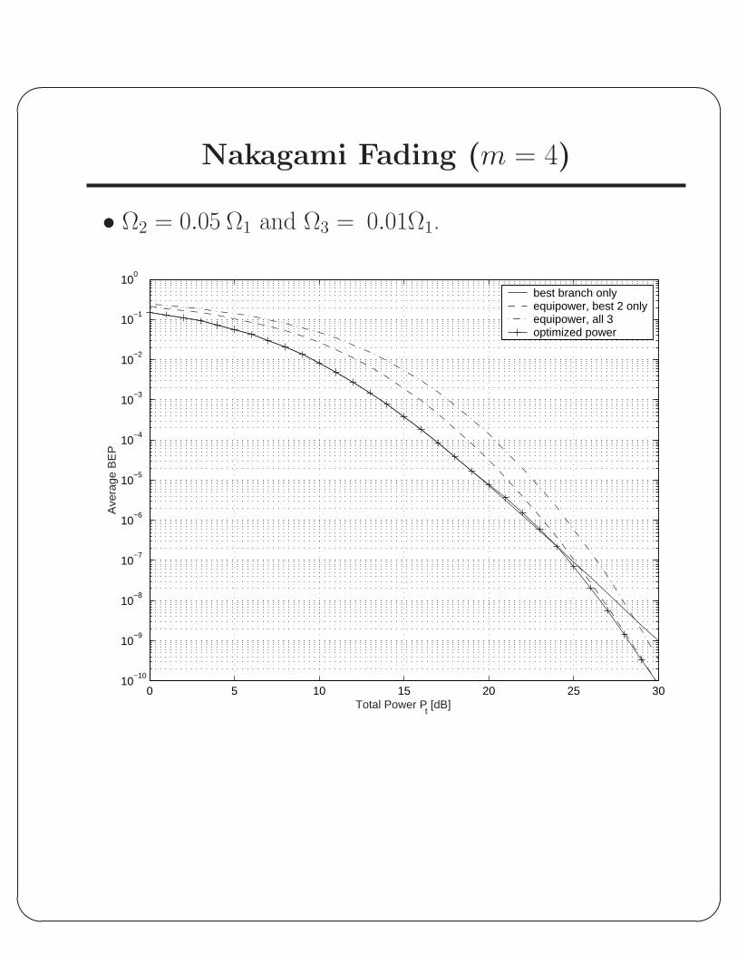
Nakagami Fading (m = 4)
• Ω2 = 0.05 Ω1 and Ω3 = 0.01Ω1.
0 5 10 15 20 25 3010
−10
10−9
10−8
10−7
10−6
10−5
10−4
10−3
10−2
10−1
100
Total Power Pt [dB]
Ave
rage
BE
P
best branch onlyequipower, best 2 onlyequipower, all 3optimized power
'
&
$
%
Model for MIMO Systems
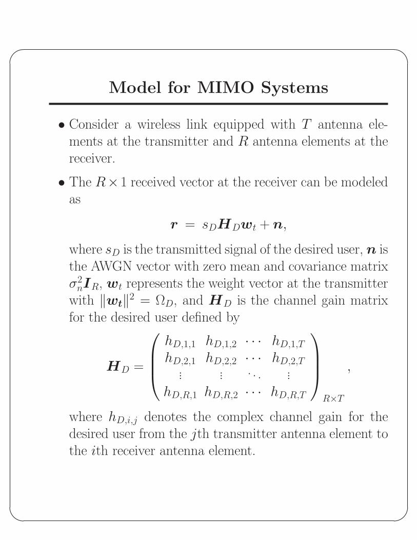
• Consider a wireless link equipped with T antenna ele-ments at the transmitter and R antenna elements at thereceiver.
• The R×1 received vector at the receiver can be modeledas
r = sDHDwt + n,
where sD is the transmitted signal of the desired user, n isthe AWGN vector with zero mean and covariance matrixσ2
nIR, wt represents the weight vector at the transmitterwith ‖wt‖2 = ΩD, and HD is the channel gain matrixfor the desired user defined by
HD =
hD,1,1 hD,1,2 · · · hD,1,T
hD,2,1 hD,2,2 · · · hD,2,T... ... . . . ...
hD,R,1 hD,R,2 · · · hD,R,T
R×T
,
where hD,i,j denotes the complex channel gain for thedesired user from the jth transmitter antenna element tothe ith receiver antenna element.

'
&
$
%
MIMO MRC Systems
• Optimum combining vector at the receiver (given thetransmitting weight vector wt) is
wr = HDwt.
• The resulting conditional (on wt) maximum SNR is
µ =1
σ2n
wHt HH
DHDwt.
• Recall the Rayleigh-Ritz Theorem:For any non-zero N × 1 complex vector x and a givenN ×N hermitian matrix A,
0 < xHAx ≤ ‖x‖2λmax,
where λmax is the largest eigenvalue of A and ‖·‖ denotesthe norm. The equality holds if and only if x is along thedirection of the eigenvector corresponding to λmax.
• Apply Rayleigh-Ritz Theorem and use transmitting weightvector as
wt =√
ΩDUmax,
where Umax (‖Umax‖ = 1) denotes the eigenvector cor-responding to the largest eigenvalue of the quadratic form
F = HHDHD.

'
&
$
%
MIMO MRC Systems (Continued)
• Maximum output SNR is given by
µ =ΩDσ2
σ2n
λmax,
where λmax is the largest eigenvalue of the matrix HHDHD,
or equivalently, the largest eigenvalue of HDHHD .
• Outage probability below a target SNR µth in i.i.d. Rayleighfading
Pout =
∣∣∣∣Ψc
(σ2
nµth
ΩDσ2
)∣∣∣∣s∏
k=1
1
Γ(t− k + 1)Γ(s− k + 1).
where s = min(T, R), t = max(T, R), and Ψc(x) is ans× s Hankel matrix function of x ∈ (0,∞) with entriesgiven by
Ψc(x)i,j = γ(t− s + i + j − 1, x),
i, j = 1, · · · , s.
and where γ(·, ·) is the incomplete gamma function.