Full Terms & Conditions of access and use can be found athttps://www.tandfonline.com/action/journalInformation?journalCode=tgis20

International Journal of Geographical InformationScience

ISSN: 1365-8816 (Print) 1362-3087 (Online) Journal homepage: https://www.tandfonline.com/loi/tgis20

An overview of clustering methods for geo-referenced time series: from one-way clustering toco- and tri-clustering

Xiaojing Wu, Changxiu Cheng, Raul Zurita-Milla & Changqing Song

To cite this article: Xiaojing Wu, Changxiu Cheng, Raul Zurita-Milla & Changqing Song (2020):An overview of clustering methods for geo-referenced time series: from one-way clusteringto co- and tri-clustering, International Journal of Geographical Information Science, DOI:10.1080/13658816.2020.1726922

To link to this article: https://doi.org/10.1080/13658816.2020.1726922

Published online: 16 Feb 2020.

Submit your article to this journal

View related articles

View Crossmark data

REVIEW ARTICLE

An overview of clustering methods for geo-referenced timeseries: from one-way clustering to co- and tri-clusteringXiaojing Wua,b,c,d, Changxiu Chenga,b,c,d, Raul Zurita-Millae and Changqing Songb,c,d

aKey Laboratory of Environmental Change and Natural Disaster, Beijing Normal University, Beijing, China;bState Key Laboratory of Earth Surface Processes and Resource Ecology, Beijing Normal University, Beijing,China; cFaculty of Geographical Science, Beijing Normal University, Beijing, China; dCenter for Geodata andAnalysis, Beijing Normal University, Beijing, China; eDepartment of Geo-Information Processing, Faculty ofGeo-Information Science and Earth Observation (ITC), University of Twente, Enschede, The Netherlands

ABSTRACTEven though many studies have shown the usefulness of clusteringfor the exploration of spatio-temporal patterns, until now there isno systematic description of clustering methods for geo-referencedtime series (GTS) classified as one-way clustering, co-clustering andtri-clustering methods. Moreover, the selection of a suitable cluster-ing method for a given dataset and task remains to be a challenge.Therefore, we present an overview of existing clustering methodsfor GTS, using the aforementioned classification, and compare dif-ferent methods to provide suggestions for the selection of appro-priate methods. For this purpose, we define a taxonomy ofclustering-related geographical questions and compare the cluster-ing methods by using representative algorithms and a case studydataset. Our results indicate that tri-clustering methods are morepowerful in exploring complex patterns at the cost of additionalcomputational effort, whereas one-way clustering and co-clusteringmethods yield less complex patterns and require less running time.However, the selection of the most suitable method should dependon the data type, research questions, computational complexity,and the availability of the methods. Finally, the described classifica-tion can include novel clustering methods, thereby enabling theexploration of more complex spatio-temporal patterns.

ARTICLE HISTORYReceived 5 June 2019Accepted 4 February 2020

KEYWORDSSpatio-temporal pattern;classification; methodselection; clustering analysis;data mining

1. Introduction

Advances in data collection and sharing techniques have resulted in significant increasesin spatio-temporal datasets. Therefore, novel approaches in terms of pattern mining andknowledge extraction are required for such large datasets (Miller and Han 2009, Chenget al. 2014, Shekhar et al. 2015). Geo-referenced time series (GTS), a type of spatio-temporal data, record time-changing values of one or more observed attributes at fixedlocations and consistent time intervals (Kisilevich et al. 2010). GTS is popular in realapplications, and examples include hourly PM2.5 concentrations observed at a networkof ground monitoring stations. Moreover, sequences of images can also be considered asGTS, e.g., satellite image time series.

CONTACT Changxiu Cheng chengcx@bnu.edu.cn

INTERNATIONAL JOURNAL OF GEOGRAPHICAL INFORMATION SCIENCEhttps://doi.org/10.1080/13658816.2020.1726922

© 2020 Informa UK Limited, trading as Taylor & Francis Group

Clustering is a data mining task that identifies similar data elements and groups themtogether. As a result, data elements in each group, or cluster, are similar to each other anddissimilar to those in other groups (Berkhin 2006, Han et al. 2012). This allows an overviewof datasets at the cluster level and also provides insights into details by focusing ona single cluster (Andrienko et al. 2009). Thus, clustering is useful for extracting patternsfrom spatio-temporal datasets.

As mentioned in previous studies (Zhao and Zaki 2005, Henriques and Madeira 2018, Wuet al. 2018), clusteringmethods for GTS can be classified as one-way clustering, co-clusteringand tri-clustering methods depending on the dimensions involved in the analysis. In sucha classification, one-way clustering methods, also termed traditional clustering, identifyclusters in one of the dimensions of 2D datasets based on the similarity of data elementsalong the other dimension (Dhillon et al. 2003, Zhao and Zaki 2005). Also analyzing 2Ddatasets, co-clustering methods identify (co-)clusters along both spatial and temporaldimensions based on the similarity of data elements along these two dimensions(Banerjee et al. 2007, Wu et al. 2020a). Tri-clustering methods identify (tri-) clusters basedon the similarity of data elements along spatial, temporal and third, e.g., attribute, dimen-sions from 3D datasets (Wu et al. 2018, Henriques andMadeira 2018). However, a systematicdescription of clustering methods for GTS from this perspective has not yet been reported.

Besides, an important issue concerns selecting appropriate clustering methods forspecific tasks at hand considering various available methods (Grubesic et al. 2014).Similar issues also exist when choosing clustering methods for GTS and we aim to providesuggestions for selecting suitable methods. To achieve this, we define a taxonomy ofclustering-related geographical questions, compare clustering methods in the aboveclassification by answering these questions using representative algorithms and a casestudy dataset, and provide suggestions for selecting suitable methods.

Thus, the objective of this study is to provide two important and unique perspectiveson clustering methods for GTS. First, we provide an overview of clustering methods forGTS using the classification outlined above. Thereafter, we compare different clusteringmethods by answering clustering-related geographical questions and provide sugges-tions on selecting suitable methods.

The structure of this paper is as follows: First, we describe the types of GTS and defineclustering-related questions in Section 2. Thereafter, we systematically describe theclustering methods for GTS in the classification in Section 3. In Section 4, our case studydataset and representative algorithms are described. Clustering results are interpretedand the algorithms are compared in Section 5. Finally, we discuss the results in Section 6and draw conclusions in Section 7.

2. GTS and questions for clustering GTS

The characteristics of the data to be analyzed heavily influence the choice of clusteringmethods (Andrienko and Andrienko 2006, Kisilevich 2010). As a type of spatio-temporaldata, GTS instinctively involves three components: space (S), time (T) and attribute (A) ina triad framework (Peuquet 1994). Depending on the number of attributes, GTS can bedivided into single attribute GTS (abbreviated to GTS-A, where A indicates the singleattribute) and multiple attributes GTS (abbreviated to GTS-As, where the affixeds indicates the plural form). Alternatively, if single attribute GTS has one attribute but two

2 X. WU ET AL.

nested hierarchies in either spatial or temporal dimension (e.g., day and hour in the caseof time), then GTS also includes the single attribute GTS with nested hierarchies in thespatial dimension (abbreviated to GTS-Ss, where the S after the hyphen indicates the spatialdimension, and s indicates the plural form) and one with nested hierarchies in the temporaldimension (abbreviated as GTS-Ts, where T after the hyphen indicates the temporal dimen-sion, and s indicates the plural form). GTS with more complex structures, e.g., with multipleattributes and nested spatial and temporal dimensions, are beyond the scope of this paperand not further discussed – also because they need the development of new clusteringmethods.

With two dimensions, GTS-A are 2D GTS and typically organized into a data table whererows are locations, columns are timestamps in which the attribute is observed, andelements of the table are values of the attribute (Figure 1(a)); for example, hourly PM2.5

concentrations recorded at monitoring stations. With three dimensions, GTS-As, GTS-Ssand GTS-Ts are 3D GTS, and any of them can be organized into a data cuboid with rows,columns and depths as its three dimensions. Take GTS-As for instance, in which rows arelocations, columns are timestamps, depths are attributes, and elements are values ofattributes observed at corresponding locations and timestamps (Figure 1(b)); for example,hourly PM2.5, PM10, NO2 and CO values recorded at monitoring stations.

In addition to the data characteristics, the other important factor for selecting cluster-ing methods is the questions researchers are interested to answer (Andrienko andAndrienko 2006). According to the triad framework developed by Peuquet (left ofFigure 2), three types of questions can be structured for GTS concerning the threecomponents: (1) where (space) + when (time) → what (attribute); (2) when + what →where; (3) where + what→ when (Peuquet 1994). For these questions, two reading levels

Figure 1. Various formats of GTS under different situations. (a) single attribute GTS (GTS-A); (b)multiple attributes GTS (GTS-As); (c) single attribute GTS with nested hierarchies in spatial dimension(GTS-Ss); (d) single attribute GTS with nested hierarchies in temporal dimension (GTS-Ts).

Figure 2. Triad framework to structure questions of the clustering analysis of GTS.

INTERNATIONAL JOURNAL OF GEOGRAPHICAL INFORMATION SCIENCE 3

are distinguished as elementary and synoptic, depending on whether the elements ofcomponents are treated individually or not (Bertin 1983, Andrienko and Andrienko 2006);for instance, questions regarding one location belong to the elementary level whereasthose regarding part of or the whole area belong to the synoptic level. Based on theaforementioned work, a taxonomy of clustering-related geographical questions is definedwith three new components: spatial-cluster (SC), temporal-cluster (TC) and cluster (C), aswell as two reading levels (right of Figure 2). Correspondingly, questions regarding onespatial-cluster belong to the elementary level while those regarding all spatial-clusters orthe subsets belong to the synoptic level. According to the taxonomy, 12 questions arestructured (Table 1).

3. Classification of clustering methods for GTS

The classification of clustering methods for GTS into one-way clustering, co- and tri-clustering methods is systematically described in this section. Each category is furtherdivided into hierarchical and partitional methods depending on whether nested clustersare created. For each type of clustering method, we first explain principles of the methodand then provide an overview of the main methods used in previous studies, emphasizingon the analysis of GTS.

Table 1. Clustering-related geographical questions.Components

Reading levels

I. where (SC) + when (TC) → what (C)Elementary SC+ elementary TC

What is the value of the cluster observed at spatial-cluster sci and timestamp-cluster tci?

Synoptic SC+ elementary TC

What is the trend of the cluster(s) observed in the whole study area at timestamp-cluster tci?

Elementary SC+ synoptic TC

What is the trend of the cluster(s) observed at location-cluster lci over the whole studyperiod?

Synoptic SC+ synoptic TC

What is the trend of the cluster(s) observed in the whole study area over the whole studyperiod?

II. when (TC) + what (C) → where (SC)Elementary TC +elementary C

At which location-cluster(s) is the cluster ci observed in timestamp-cluster tci?

Synoptic TC+ elementary C

At which location-cluster(s) is the cluster ci observed over the whole study period?

Elementary TC+ synoptic C

At which location-cluster(s) are all clusters observed in timestamp-cluster tci?

Synoptic TC+ synoptic C

At which location-cluster(s) are all clusters observed over the whole time period?

III. where (SC) + what (C) → when (TC)Elementary SC +elementary C

In which timestamp-cluster(s) is the cluster ci observed at location-cluster li?

Synoptic SC +elementary C

In which timestamp-cluster(s) is the cluster ci observed in the whole study area?

Elementary SC +synoptic C

In which timestamp-cluster(s) are all clusters observed at location-cluster li?

Synoptic SC +synoptic C

In which timestamp-cluster(s) are all clusters observed in the whole study area?

4 X. WU ET AL.

3.1. One-way clustering methods

Both traditional partitional and hierarchical clusteringmethods analyze 2DGTS organized intothe table either from the spatial or the temporal perspective, respectively. For example,traditional partitional clustering methods regard locations as objects and timestamps asattributes when analyzing from the spatial perspective (Figure 3(b1)). Then, they partitionlocations into location-clusters, based on the similarity of data elements across all timestamps.As the clustering results are location-clusters, such an analysis is also known as spatialpartitional clustering. When analyzing from the temporal perspective (Figure 3(b2)), tradi-tional partitional clusteringmethods regard timestamps as objects and locations as attributes.Subsequently, they partition timestamps into timestamp-clusters based on the similarity ofelements across all locations. Such an analysis is also known as temporal partitional clusteringbecause the resulting clusters are timestamp-clusters. Theoretically, any traditional clusteringmethod can perform spatial and temporal clustering analysis separately.

3.1.1. Overview of traditional clustering methodsExtensive studies have been conducted for the application of clusteringmethods for spatio-temporal data, including GTS (Berkhin 2006, Han et al. 2012), most of which are traditionalmethods. Regarding traditional partitional clustering algorithms, the most widely used oneis k-means (MacQueen 1967, Lloyd 1982). This algorithm is described in detail as beingrepresentative of one-way clustering methods (Section 4.2). White et al. (2005) and Millset al. (2011) employed k-means to locate similar regions in terms of phenology. Usinga partitioning and optimization process similar to that of k-means, iterative self-organizingdata analysis (ISODATA) employs the predefined number of clusters as an initial estimate,and it is able to delete, split, and merge clusters for further refinement (Tou and Gonzalez1974). Gu et al. (2010) applied ISODATA, which is widely used in remote sensing, to identify

Figure 3. Partitional clustering methods for GTS: (a&b1&b2) one-way clustering, (a&c) co-clusteringand (d&e) tri-clustering.

INTERNATIONAL JOURNAL OF GEOGRAPHICAL INFORMATION SCIENCE 5

regions with similar phenological characteristics. Kohonen (1995) developed self-organizingmaps (SOM) to map n-dimensional input data to neurons on a 2D plane. Starting witha random initialization of values for the neurons, SOM considers each input data as a vectorand aims to determine its best match unit (BMU) in the neurons with the nearest Euclideandistance. Once chosen as a BMU of a particular vector, the neuron changes the values of itsneighboring neurons in the output space by using a neighborhood function. The above-mentioned training process ceases when all the input vectors find their correspondingBMUs, and the output neurons become stable. Thus, SOM groups similar input vectors tothe same or adjacent neurons, thereby proving their feasibility for partitional clusteringanalysis. Owing to its effectiveness for dimension reduction, SOM has also been used forspatial or temporal clustering in many applications such as company location (Guo et al.2006), crime rate analysis (Andrienko et al. 2010), and weather analysis (Wu et al. 2013).

In terms of traditional hierarchical clustering methods, popular algorithms arebalanced iterative reducing and clustering using hierarchies (BIRCH, Zhang et al.1996) and hierarchical SOM (Hagenauer and Helbich 2013). Designed for clusteringlarge datasets, BIRCH first extracts the clustering features (CFs) from data and thenorganizes the CFs into a clustering feature tree (CF tree). Then, the next optional stepentails compressing the initial CF tree into a smaller one to remove outliers and groupsub-clusters. Once the smaller CF tree is built, BIRCH uses an existing hierarchicalclustering algorithm to conduct global clustering with the CF tree. The final optionalstep is to reassign data elements to the closest existing cluster centroids to refine theclusters. Inspired by previous work on Kangas Map (KM, Kangas 1992, Bação et al.2005) and SOM, Hagenauer and Helbich (2013) proposed a hierarchical clusteringalgorithm named hierarchical spatio-temporal SOM (HSTSOM), which is designed witha spatial and temporal KM in the upper layer and a basic SOM in the lower layer. Toseparately consider the spatial and temporal dependence of the data, HSTSOM trainsthe two KMs in the upper layer independently but in parallel. To identify spatio-temporal clusters, this algorithm then concatenates the positions of BMUs in theupper-layer KMs for each input data to create training vectors for the lower-layerSOM. In their study, HSTSOM was applied to analyze the socio-economic character-istics of Vienna. Additional traditional clustering methods are discussed in the litera-ture (Berkhin 2006, Miller and Han 2009, Grubesic et al. 2014).

3.2. Co-clustering methods

Both partitional and hierarchical co-clustering methods treat locations and timestampsequally and concurrently analyze 2D GTS along the spatial and temporal dimensions. Forexample, partitional co-clustering methods (Figure 3(c)) simultaneously partition loca-tions into location-clusters and timestamps into timestamp-clusters based on the simi-larity of data elements along both locations and timestamps. In this case, the clusteringresults are co-clusters with similar elements along both dimensions, which are intersectedby each of location-clusters and timestamp-clusters.

3.2.1. Overview of co-clustering methodsCo-clustering methods have attracted significant attention ever since they were firstproposed in the early 1970s (Hartigan 1972, Padilha and Campello 2017, Shen et al.

6 X. WU ET AL.

2018, Wu et al. 2020b). However, the majority of previous studies focused on other fields,especially bioinformatics (Eren et al. 2012), with only a few recent studies focusing onspatio-temporal data (Wu et al. 2017). To ensure our overview is comprehensive, co-clustering methods used in other fields are also mentioned here.

Regarding partitional co-clustering methods, Dhillon et al. (2003) proposed the informa-tion theoretic co-clustering (ITCC) algorithm for simultaneous word-document clustering.With an initial random mapping from words to word-clusters and document to document-clusters, ITCC regards the co-clustering issue as the optimization process in informationtheory and formulates the objective function as the loss of mutual information between theoriginal variables (word and document) and the clustered ones (word-clusters and docu-ment-clusters). Then, it optimizes the objective function by reassigning words and docu-ments to word-clusters and document-clusters until convergence is achieved. Cho et al.(2004), who aimed to analyze gene expression data, developed a co-clustering algorithm byusing the minimum sum-squared residual as the similarity/dissimilarity measure. This algo-rithm organizes data in the form of a 2D matrix and yields the first set of row-clusters andcolumn-clusters using either random or spectral initialization, and uses residuals to buildthe objective function, which it then minimizes to obtain the optimal co-clustering results.Generalizing these previous studies (Dhillon et al. 2003, Cho et al. 2004), Banerjee et al.(2007) subsequently proposed the Bregman co-clustering algorithm as a meta co-clusteringalgorithm that aims to partition the original data into co-clusters with several distortionfunctions such as the Euclidean distance. They also mentioned several applications of co-clustering such as natural language processing (Rohwer and Freitag 2004) and videocontent analysis (Cai et al. 2005). Recently, Wu et al. (2015) applied the Bregman blockaverage co-clustering algorithm with I-divergence (BBAC_I), a special case of the Bregmanco-clustering algorithm, to analyze temperature series for simultaneous location and time-stamp clustering. This was the first study that applied co-clustering analysis to spatio-temporal data. Afterwards, several studies applied BBAC_I for analyzing GTS in a varietyof fields, for example, disease hotspot detection (Ullah et al. 2017) and identification offavorable conditions for virus outbreaks (Andreo et al. 2018).

Regarding hierarchical co-clustering methods, Hartigan (1972) developed a direct co-clustering algorithm and applied it to analyze American presidential voting. This algo-rithm, which is one of the earliest co-clustering algorithms, employs the squaredEuclidean distance to build the objective function and then aims to minimize it byusing a ‘divide and conquer’ direct clustering algorithm in a hierarchical manner.Another hierarchical co-clustering algorithm proposed by Hosseini and Abolhassani(2007) aimed to analyze queries and URLs of a search engine log, to mine the querylogs in web information systems. This algorithm uses the queries and URLs to constructa bipartite graph in which singular value decomposition (SVD) is used to perform dimen-sion reduction. Subsequently, k-means is used to iteratively cluster queries, and URLs areused to create the hierarchical categorization. Costa et al. (2008) developed a hierarchical,model-based co-clustering algorithm and used it to analyze internet advertisements.Considering the dataset as a joint probability distribution, this algorithm groups tuplesinto clusters characterized by different probability distributions. Thereafter, co-clusters areidentified by exploring the conditional distribution of elements over tuples. Inspired byITCC, Cheng et al. (2012), and Cheng et al. (2016) proposed a hierarchical co-clusteringalgorithm by employing the information divergence as the measure of similarity/

INTERNATIONAL JOURNAL OF GEOGRAPHICAL INFORMATION SCIENCE 7

dissimilarity to analyze newsgroups and documents. This algorithm starts with an initialco-cluster, and then constructs hierarchical structures of rows and columns by iterativelysplitting the rows and columns to achieve convergence. Unlike ITCC, which uses the lossin mutual information, Ienco et al. (2009) and Pensa et al. (2012) proposed a hierarchicalco-clustering algorithm named Incremental Flat and Hierarchical Co-Clustering (iHiCC).This algorithm employs Goodman-Kruskal’s τ coefficient to measure the strength of thelink between two variables and uses the result for text categorization. Using the firsthierarchy created by τCoClust (Robardet 2002), this algorithm divides rows and columnsiteratively until only one element remains in all leaves of the hierarchies of both rows andcolumns. However, to date, studies that have applied hierarchical co-clustering methodsfor the analysis of spatio-temporal data have not been published. Detailed reviews on co-clustering were presented by Charrad and Ahmed (2011), Eren et al. (2012), and Padilhaand Campello (2017).

3.3. Tri-clustering methods

Both partitional and hierarchical tri-clustering methods concurrently analyze 3D GTS inthe cuboid along the spatial, temporal, and third dimensions. For example, partitional tri-clustering analysis of GTS-As (Figure 3(e)) simultaneously groups locations into location-clusters, timestamps into timestamp-clusters and attributes into attribute-clusters basedon the similarity of data elements along all three dimensions. The clustering results are tri-clusters that contain similar elements along locations, timestamps and attributes, whichare intersected by each of location-clusters, timestamp-clusters, and attribute-clusters.

3.3.1. Overview of tri-clustering methodsSince the proposal of the first tri-clustering algorithm in 2005 (Zhao and Zaki 2005), thisemerging subject has attracted increasing attention (Henriques and Madeira 2018).Almost all previous studies on tri-clustering methods focused on other fields, with fewon geo-related fields (Wu et al. 2018). Nevertheless, we mention other methods to ensureour description is complete.

Previous studies focused on partitional tri-clustering methods to a larger extent. Zhao andZaki (2005) introduced the first tri-clustering algorithm named TRICLUSTER, which aims tomine coherent gene expression over time based on graph-based approaches. TRICLUSTERfirst identifies co-clusters as the intermediate results by creating multigraphs of ranges andfinding constrained maximal cliques. Subsequently, these candidate co-clusters generate tri-clusters. Thereafter, Sim et al. (2010) proposed the mining-correlated 3D subspace Cluster(MIC) to analyze continuous-valued data and stock-financial-ratio-year data as examples.Initialized by generating pairs of values with highly correlated information as seeds or initialclusters, MIC greedily refines these clusters to mine correlated 3D subspace clusters byoptimizing the correlation information of those seeds. In addition, Hu and Bhatnagar (2010)proposed a tri-clustering algorithm to analyze real-valued gene expression data. Their algo-rithm identifies tri-clusters in two datasets by specifying an upper threshold for the standarddeviations of these tri-clusters. To this end, the algorithm first searches for co-clusters of whichthe standard deviation obeys the specified upper bound in each dataset. Then, tri-clusters areformulated from these candidate co-clusters. Based on their work on co-clustering analysis,Wu et al. (2018) extended an existing co-clustering algorithm to a tri-clustering algorithm

8 X. WU ET AL.

named the Bregman cuboid average tri-clustering algorithm with I-divergence (BCAT_I) toanalyze 3D GTS.

Few studies concerned with hierarchical tri-clustering methods have been reportedand these efforts mostly focus on analyzing biological data. Gerber et al. (2007) developeda tri-clustering algorithm named GeneProgram for gene expression data analysis basedon hierarchical Dirichlet processes. This algorithm first discretizes continuous geneexpression data, and then employs Markov chain Monte Carlo sampling to approximatethe model posterior probability distribution using a three-level hierarchy in the Dirichletprocess, and finally identifies tri-clusters by summarizing the distribution. Amar et al.(2015) proposed an algorithm known as three-way module inference via Gibbs sampling(TWIGS) to analyze large 3D biological datasets. TWIGS functions by initially developinga hierarchical Bayesian generative model for binary data by using the Bernoulli-Betaassumption and for real-valued data by using the Normal-Gamma assumption.Subsequently, TWIGS employs a co-clustering solution as the starting point and theniteratively improves it using the Gibbs sampler. Finally, tri-clusters are inferred fromcandidate co-clusters. A detailed overview of tri-clustering algorithms was published byHenriques and Madeira (2018).

4. Data and representative algorithms of clustering methods

In this section, the dataset we used as a case study is first described. Then, algorithmsrepresentative of each category of clustering methods are briefly described.

4.1. Case study dataset

To illustrate this study, we used the PM2.5 dataset published by Microsoft Research Asia(MRA, Zheng et al. 2013, 2014), which is freely available. The dataset contains hourly PM2.5

concentrations at 36 monitoring stations in Beijing from 8 February 2013 to8 February 2014. Because of the incompleteness of the dataset (Li et al. 2016), we selected18 stations in the central urban areas (Figure 4). A Thiessen polygon map was createdusing the coordinates of these stations (also available from MRA) to indicate the areacovered by each station. Furthermore, for the purpose of analysis, 299 days ranging from1 February 2013 to 31 January 2014 (365 days) were selected as the study period with thecriterion that the days on which PM2.5 concentrations for all stations are zero for 24 h areremoved. The temporal distribution of these 299 days and the number of non-zero days ineach month over the study period are shown in Figure 5. The experiments were imple-mented in MATLAB 2018a on a laptop running Windows 10 (64-bit) with a 2.20-GHz Intelcore (i7) CPU with 16 GB of RAM. Parallel computing was not implemented in ourexperiments although this could be an interesting line for further research.

Patterns of spatial distribution, seasonal and diurnal variation of PM2.5 concentrationswere analyzed in previous studies (Zhang and Cao 2015, Chen et al. 2015). Based on theseexisting studies, we constructed example questions for the PM2.5 dataset according to theclustering-related questions discussed in Section 2. The 22 example questions we con-structed are listed in Table 2. Clustering methods were then compared by answeringthese questions.

INTERNATIONAL JOURNAL OF GEOGRAPHICAL INFORMATION SCIENCE 9

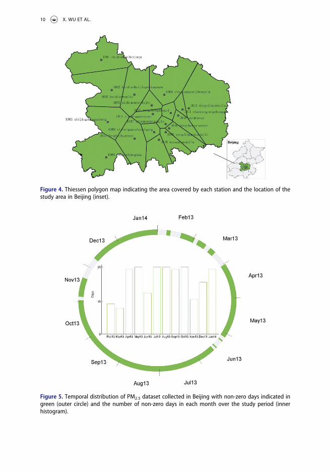
Figure 4. Thiessen polygon map indicating the area covered by each station and the location of thestudy area in Beijing (inset).

Figure 5. Temporal distribution of PM2.5 dataset collected in Beijing with non-zero days indicated ingreen (outer circle) and the number of non-zero days in each month over the study period (innerhistogram).

10 X. WU ET AL.

4.2. K-means

Since the case study dataset is an hourly PM2.5 dataset, i.e., single attribute GTS with dayand hour as nested temporal dimensions (GTS-Ts), it was averaged to daily PM2.5 dataset,i.e., single attribute GTS (GTS-A) when subjected to the traditional clustering method. Thedataset is organized into a table where rows are stations, columns are days and elementsare daily PM2.5 concentrations. Such a data table could also be seen as the co-occurrencematrix OSD between a spatial and temporal variable, the former taking values in m (18)stations and the latter in n (299) days.

Because of its wide use in many applications (Berkhin 2006), k-means was selected asthe algorithm representative of traditional clustering methods and used in this study toperform temporal clustering. It is noteworthy that k-means can also be used to performspatial clustering.

Table 2. Example questions of the clustering PM2.5 dataset in Beijing.Components

Reading levels Number

I. where (SC) + when (TC) → what (C)elementary SC+ elementary TC

What is/are the pollution level(s) of PM2.5 at station-cluster1 and in day-cluster1? 1What is/are the pollution level(s) of PM2.5 at station-cluster1, in day-cluster1 andin hour-cluster1?

2

synoptic SC+ elementary TC

What is the pattern of pollution in the study area in day-cluster2? 3What is the pattern of pollution in the study area in day-cluster1 and hour-cluster1? 4

Elementary SC+ synoptic TC

What is the pattern of pollution at station-cluster1 over the study period? 5

synoptic SC+ synoptic TC

What is the seasonal distribution of the pollution in the study area over the studyperiod?

6

What is the spatial distribution and seasonal variation of the pollution in the studyarea over the study period?

7

What is the spatial distribution, seasonal and diurnal variation of the pollution in thestudy area over the study period?

8

II. when (TC) + what (C) → where (SC)elementary TC +elementary C

At which station-cluster(s) is the PM2.5 pollution level of Good observed in day-cluster2?

9

At which station-cluster(s) is the PM2.5 pollution level of Good observed in day-cluster2 and hour-cluster1?

10

Synoptic TC+ elementary C

At which station-cluster(s) is the PM2.5 pollution level of Good observed over thestudy period?

11

elementary TC+ synoptic C

At which station-cluster(s) is the PM2.5 pollution level becoming worse in day-cluster1? 12At which station-cluster(s) is the PM2.5 pollution level becoming worse in day-cluster2 and hour-cluster1?

13

Synoptic TC+ synoptic C

At which station-cluster(s) is the PM2.5 pollution level becoming worse over the timeperiod?

14

III. where (SC) + what (C) → when (TC)elementary SC+elementary C

In which day-cluster(s) is the PM2.5 pollution level of Good observed at station-cluster1?

15

In which day-cluster(s) and hour-cluster(s) is the PM2.5 pollution level of Goodobserved at station-cluster1?

16

synoptic SC +elementary C

In which day-cluster(s) is the PM2.5 pollution level of Good observed in the studyarea?

17

In which day-cluster(s) and hour-cluster(s) is the PM2.5 pollution level of Goodobserved in the study area?

18

elementary SC +synoptic C

In which day-cluster(s) does the PM2.5 pollution level worsen at station-cluster1? 19In which day-cluster(s) and hour-clusters does the PM2.5 pollution level worsen atstation-cluster1?

20

synoptic SC +synoptic C

In which day-cluster(s) does the PM2.5 pollution level worsen in the study area? 21In which day-cluster(s) and hour-cluster(s) does the PM2.5 pollution level worsen inthe study area?

22

INTERNATIONAL JOURNAL OF GEOGRAPHICAL INFORMATION SCIENCE 11

Suppose the days are clustered into l day-clusters. The pseudocode of the process ofiteratively optimizing day-clusters by k-means is depicted in Figure 6. With a randominitialization, l days are first selected as the cluster centers (step 1). Then, the iterativeprocess starts by assigning each of n days to the most similar cluster center measured bythe Euclidean distance indicated by Deucð; Þ(step 2.1). Next, for each of l day-clusters, thecluster center is updated as the mean of all days assigned to this cluster (step 2.2). Theobjective function of k-means is typically formulated as the sum of squared errorsbetween the days and corresponding day-clusters. The iterative process continues untilthe objective function converges (i.e. reaches a value below a predefined threshold) andthe optimized l day-clusters are yielded.

4.3. Bregman block average co-clustering algorithm with I-divergence (BBAC_I)

The co-clustering method was also used to analyze the daily PM2.5 dataset in the table andconsiders the table as the co-occurrence matrix, OSD. BBAC_I was chosen as the repre-sentative algorithm because of its effectiveness in analyzing GTS (Wu et al. 2015, 2016).

Suppose the stations are clustered into k station-clusters, and the days are clusteredinto l day-clusters for the analysis of the daily PM2.5 data matrix, OSD. The pseudocode ofBBAC_I (shown in Figure 7) demonstrates the process of optimizing the station-clustersand day-clusters iteratively. With a random initial mapping as the starting point (step 1),stations are partitioned into k station-clusters and days into l day-clusters concurrently,resulting in a co-clustered 2D data matrix (OSD). The objective function is then formulatedas the distortion between the original and the co-clustered matrices measured using the

Figure 6. Pseudocode of the k-means algorithm.

12 X. WU ET AL.

information divergence (step 2), where DIð�jj�Þ indicates the information divergence oftwo matrices. Thereafter, the iterative process starts by re-assigning stations to station-clusters and days to day-clusters, to optimize the objective function (step 3). This processhas been proven to monotonically decrease the objective function after each reassign-ment (Banerjee et al. 2007). The iterative process terminates when the objective functionachieves convergence (i.e., gets below a predefined threshold) and k × l optimized sta-tion-day co-clusters are yielded.

4.4. Bregman cuboid average tri-clustering algorithm with I-divergence (BCAT_I)

The tri-clustering method was used to analyze the hourly PM2.5 dataset, which is orga-nized into a data cuboid where rows represent stations, columns represent days, depthsare 24 hours, and elements are hourly PM2.5 concentrations. Such a data cuboid can beregarded as the 3D co-occurrence matrix, OSDH, among one spatial variable taking valuesin m (18) stations, and two temporal variables, taking values in n (299) days and p (24)hours, respectively.

BCAT_I, which was developed and proven to be effective for analyzing GTS (Wu et al.2018), was selected as the representative algorithm. Suppose the stations, days and24 hours in OSDH are clustered into k station-clusters, l day-clusters and z hour-clusters inthe tri-clustering analysis. The pseudocode of BCAT_I (Figure 8) demonstrates the

Figure 7. Pseudocode of BBAC_I.

INTERNATIONAL JOURNAL OF GEOGRAPHICAL INFORMATION SCIENCE 13

optimization process of partitioning the hourly PM2.5 matrix into tri-clusters in an iterativemanner. Starting with a random initialization by mapping stations to k station-clusters, daysto l day-clusters and hours to z hour-clusters (step1), the algorithm first generates a tri-clustered 3D data matrix (OSDH). In the next step, BCAT_I measures the distortion betweenthe original and the tri-clustered matrices using the information divergence to build itsobjective function (step 2). Thereafter, it aims to minimize the objective function byiteratively updating mappings from stations to station-clusters, days to day-clusters andhours to hour-clusters (step 3). The iterative process ceases when the objective function isbelow a preset threshold, which yields the optimized k × l × z station-day-hour tri-clusters.

5. Results

In our analysis, the number of station-clusters was chosen to be three in accordance withprevious studies (Zhao et al. 2014, Wang et al. 2015) and the number of day-clusters is setas four, with the expectation that days would fall into four ‘real’ seasons to enable us toexplore patterns of seasonal variations. Additionally, the number of hour-clusters was set

Figure 8. Pseudocode of BCAT_I.

14 X. WU ET AL.

to six because the air pollution index (AQI) for PM2.5 is categorized into six levels: Excellent(0–50), Good (51–100), Lightly polluted (101–150), Moderately polluted (151–200), Heavilypolluted (201–300) and Severely polluted (>300) (according to the Technical Regulationon Ambient Air Quality Index (on Trial) (China 2012)). Clustering results are interpreted byanswering example questions for clustering the PM2.5 dataset and then the three cluster-ing algorithms are compared in terms of several aspects.

5.1. K-means clustering results

After the temporal clustering analysis, the 299 days are grouped into four day-clusters.The ringmap in Figure 9 displays the temporal distribution of the four clusters of days. Theinnermost circle in the ringmap shows the distribution of zero values in 365 days and theother four circles are four clusters of days with increasing concentrations from inside

Figure 9. Ringmap displaying the results of k-means clustering. The innermost circle indicating dayswith zero values. Other four circles from inside outward indicating day-cluster 1 to day-cluster 4 anddays in each day-cluster colored the same using average value.

INTERNATIONAL JOURNAL OF GEOGRAPHICAL INFORMATION SCIENCE 15

outward. Each circle indicates 365 days, which is divided into 12 months fromFebruary 2013 to January 2014 in a clockwise direction, and days falling into each clusterare colored using the average value of that cluster.

With the ringmap, four out of the 22 questions (numbers: 3, 6, 17, 21) can be answered.In response to question number 3, the ringmap shows that day-cluster2 has the averagedvalue of ‘Lightly polluted’ according to (China 2012) and days therein mainly occur inSpring (April and May), Summer and early Autumn (July, August, September and October).As for question number 6, it can be seen that ‘Good’ days in day-cluster1 are sparselyspread in April, July, August, December and January while ‘Lightly polluted’ days occupymost of the study area. ‘Heavily polluted’ days are scattered throughout Winter and alsoOctober. In response to question number 16, days in day-cluster4 are ‘Heavily polluted,’and the fewest days are scattered throughout January 2014, February, early March andOctober. For question number 20, because day-clusters are arranged from 1 to 4 withincreasing values of PM2.5 concentrations, the pollution level becomes worse from day-cluster1 to day-cluster4.

5.2. BBAC_I co-clustering results

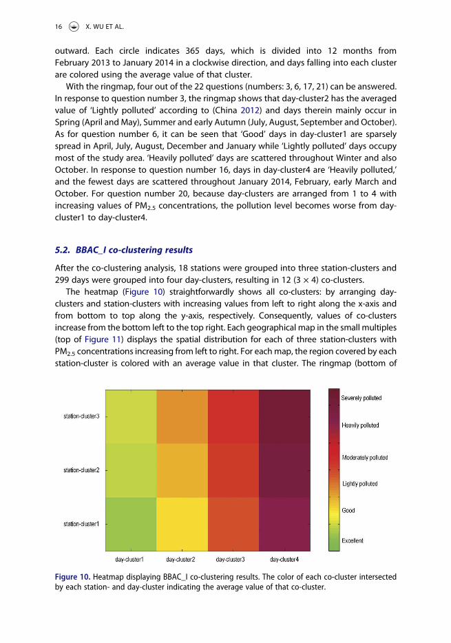
After the co-clustering analysis, 18 stations were grouped into three station-clusters and299 days were grouped into four day-clusters, resulting in 12 (3 × 4) co-clusters.

The heatmap (Figure 10) straightforwardly shows all co-clusters: by arranging day-clusters and station-clusters with increasing values from left to right along the x-axis andfrom bottom to top along the y-axis, respectively. Consequently, values of co-clustersincrease from the bottom left to the top right. Each geographical map in the small multiples(top of Figure 11) displays the spatial distribution for each of three station-clusters withPM2.5 concentrations increasing from left to right. For eachmap, the region covered by eachstation-cluster is colored with an average value in that cluster. The ringmap (bottom of

Figure 10. Heatmap displaying BBAC_I co-clustering results. The color of each co-cluster intersectedby each station- and day-cluster indicating the average value of that co-cluster.

16 X. WU ET AL.

Figure 11) shows the temporal distribution of four day-clusters using four circles insideoutward with increasing values. For each circle, days in corresponding day-clusters aredisplayed in the same color as an average value.

With these visualizations, more than half of the example questions (13) can beanswered (numbers: 1, 3, 5, 6, 7, 9, 11, 12, 14, 15, 17, 19, 21). Questions answered byk-means clustering results are not repeated. For question number 1, the heatmap shows

Figure 11. Small multiples (top) and ringmap (bottom) displaying BBAC_I co-clustering results. In thesmall multiples, stations falling into each station-cluster colored using the average value of thatstation-cluster. In the ringmap, the innermost circle indicating days with zero values. Other four circles,from inside outward, representing day-cluster1 to day-cluster4 and days in each day-cluster coloredthe same as the average value.

INTERNATIONAL JOURNAL OF GEOGRAPHICAL INFORMATION SCIENCE 17

that the co-cluster intersected by station-cluster1 and day-cluster4 is ‘Heavily polluted’.For question number 3, days in day-cluster2 are mostly spread from July to October.During these days, the pollution level worsens from ‘Good’ at stations in the east (station-cluster1&2) to ‘Lightly polluted’ at stations in the west (station-cluster3). In response toquestion number 5, the pollution level of the Haidianbeijingzhiwuyuan station (1002, 海淀北京植物园) in station-cluster1 changes from ‘Excellent’ in day-cluster1 to ‘Heavilypolluted’ in day-cluster4. For question number 7, the pollution level worsens from thewest to the east of the study area and from Summer to Winter in the study period.Moreover, the highest fluctuations of PM2.5 values occur during Winter, with the highestand lowest levels of the entire year, whereas the fluctuations in Spring and Summer aremuch reduced with medium-level concentrations (Li et al. 2015, 2016). For questionnumber 9, the heatmap shows that in station-cluster1, the pollution level of ‘Good’ isobserved in day-cluster2. The result also shows that in station-cluster1 and station-cluster2, the pollution level is observed to be ‘Good’ over the study period as the responseto question number 11. For question number 12, in day-cluster1, the pollution levelworsens from station-cluster1 in the west to station-cluster3 in the east of the studyarea. The same trend can also be observed over the time period for question number 14.The answer to question number 15 is the same as that to question number 9 and theanswer to the last question is the same as that to question number 5.

5.3. BCAT_I tri-clustering results

After the tri-clustering analysis, 18 stations, 299 days and 24 hours were grouped intothree station-clusters, four day-clusters and six hour-clusters, respectively, resulting in72 (3 × 4 × 6) tri-clusters. The quasi-3D heatmap in Figure 12 provides a direct view of alltri-clusters arranged according to station-clusters, day-clusters, and hour-clusters withvalues increasing from bottom to top of rows, from left to right of columns, and fromfront to back of the depths, respectively. The overall view is that the values of tri-clustersincrease from the bottom left front to the top right back. The spatial distribution foreach station-cluster is displayed in the small multiples with PM2.5 values increasing fromleft to right (top of Figure 13). Four circles in the ringmap (middle of Figure 13) usecolors to display the temporal distribution of days in four day-cluster with valuesincreasing from the innermost to the outermost ring. The set of six bar timelines(bottom of Figure 13) displays the temporal distribution of six hour-cluster over24 hours with concentrations increasing from the bottom to the top. Each bar timelinerepresents 24 hours and hours in each hour-cluster are colored using the average valueof that hour-cluster to show the distribution.

With the above visualizations, all example questions can be answered. Questions thatwere answered by k-means and co-clustering results are not repeated. For questionnumber 2, the quasi-3D heatmap shows that the pollution level of PM2.5 is ‘Excellent’ atstation-cluster1, day-cluster1 and hour-cluster1. For question number 4, the overallpollution level in day-cluster1 and hour-cluster1 is ‘Excellent’ with the pollution slightlyworsening from the west to the east of the study area. For question number 8, thecombination of visualizations shows that most stations in the west and other stationsmostly in the southern and eastern areas have the highest value. These results areconsistent with those of previous studies, i.e., low PM2.5 values exist in the north (west),

18 X. WU ET AL.

whereas high values exist in the south (east) (Zhao et al. 2014, Wang et al. 2015). Withrespect to the seasonal variation, it is shown that high fluctuations of PM2.5 concentrationsoccur in the Autumn and especially in the Winter, whereas a more stable pattern ofmiddle-valued concentrations appear in the Spring and Summer (Li et al. 2015, 2016).Furthermore, hours from 7:00 to 14:00 are characterized by low concentrations, whereashours from 21:00 to 24:00 and 1:00 to 3:00 occur the highest PM2.5 concentrations. Theseresults are supported by previous studies on diurnal variations (Zhao et al. 2014, Chenet al. 2015). For question number 10, the heatmap shows that in day-cluster2 and hour-cluster1, station-cluster2 and station-cluster3 are observed to have a ‘Good’ pollutionlevel. This includes all stations except Haidianbeijingzhiwuyuan (1002, 海淀北京植物园)as shown in the small multiples. The response to question number 13 is that, in day-cluster2 and hour-cluster1, the pollution level worsens from ‘Excellent’ to ‘Good’ fromstation-cluster1 to station-clusters2&3. For question number 16, the heatmap shows that,in station-cluster1, the pollution level is observed to be ‘Good’ at several intersectionsof day-clusters and hour-clusters, e.g., the intersections of day-cluster1 and hour-cluster6,day-cluster2 and hour-cluster2. It also shows that the pollution level of ‘Good’ is observedat additional intersections of day-clusters and hour-clusters in the study area for questionnumber 18 (e.g., that of day-cluster2 and hour-clusters1-6 at station-cluster3). For ques-tion number 20, at station-cluster1, the pollution level worsens from day-cluster1and hour-cluster1 to day-cluster4 and hour-cluster6, i.e., from hours 7:00–9:00 on daysscattered throughout April and November to hours 21:00–24:00 on days spread sparselyacross September, October and January 2014. Moreover, it shows that the pollution level

Figure 12. Quasi-3D heatmap displaying the tri-clustering results. The color of each tri-clusterintersected by each station-, day- and hour-cluster indicating the average value of that tri-cluster.

INTERNATIONAL JOURNAL OF GEOGRAPHICAL INFORMATION SCIENCE 19

Figure 13. Small multiples (top), ringmap (middle) and bar timelines (bottom) displaying the tri-clusteringresults. In the small multiples, stations in each station-cluster colored the same using average value. In theringmap, the innermost circle indicating days with zero values. Other four circles (from inside outward)indicating day-cluster1 to day-cluster4 and days in each day-cluster colored the same using average value.In the bar timelines, hours in each hour-cluster colored the same using average value.

20 X. WU ET AL.

is worsening from day-cluster1, hour-cluster1 and station-cluster1 to day-cluster4, hour-cluster6 and station-cluster3, respectively, in response to the last question.

5.4. Comparisons of clustering algorithms

The k-means, BBAC_I and BCAT_I algorithms are compared using the case study datasetand the results in terms of the input data, size of the data matrix, the number ofparameters needed, the number of iterations & initializations, computational efficiencyrepresented by average running time and also the number of example questionsanswered (Table 3).

The results in Table 3 indicate that BCAT_I analyzes the dataset with finer resolutionand larger size than k-means and BBAC_I, whereas BCAT_I requires a larger number ofinput parameters. Both k-means and BBAC_I analyzed the daily PM2.5 dataset with the size18 × 299, whereas BCAT_I analyzed the hourly dataset with the size 18 × 299 × 24. As such,the tri-clustering algorithm allows the inclusion of more information in the clusteringprocess and consequently in the results. In terms of the number of input parameters forthe case study, k-means requires the least, namely three, i.e., the number of day-clusters,iterations and initializations. In comparison, BBAC_I needs an additional parameter as thenumber of station-clusters and BCAT_I also needs the number of hour-clusters.

In terms of computational efficiency, k-means requires the shortest average running timefor analysis in the case study, followed by BBAC_I, whereas BCAT_I needs the longest time.Using the same number of iterations and initializations for each algorithm, the results inTable 3 indicate that k-means is 100 times faster than BBAC_I and thousands of times fasterthan BCAT_I. Compared with BCAT_I, the average running time of BBAC_I is 60 times faster.

In terms of answering example questions, BCAT_I is the most capable method becauseit allows us to answer all questions. This method is followed by BBAC_I (answers morethan half of all questions), and then k-means (answers less than one-fifth of all questions).By performing temporal clustering, k-means can answer any question on the spatial-cluster at the synoptic level (synoptic SC). Because traditional clustering methods canperform spatial clustering separately, theoretically k-means can also answer three exam-ple questions: 5, 11 and 14 (which are questions on the temporal-cluster at the synopticlevel (synoptic TC)). As such, it can reveal spatial or temporal patterns, e.g., the seasonalvariation in the PM2.5 dataset. BBAC_I concurrently performed spatial and temporalclustering with the clustering results allowing us to answer all questions except thosewith two nested temporal dimensions. In view of this, BBAC_I can reveal more complexpatterns, e.g., the spatial distribution and seasonal variation in the case study dataset. Theanalysis of the hourly dataset using BCAT_I enabled us to answer all questions and exploremore patterns in the dataset, e.g., the spatial distribution, seasonal and diurnal variations.

Table 3. Comparisons of the three clustering algorithms.

Clusteringalgorithm Input data

Size of thedata matrix

Number ofparametersneeded

Number ofiterations &initializations

Averagerunningtime

Number of exam-ple questionsanswered

k-means Daily PM2.5 dataset 18 × 299 3 100 & 20 0.01 second 4 (out of 22)BBAC_I Daily PM2.5 dataset 18 × 299 4 100 & 20 1 second 13 (out of 22)BCAT_I Hourly PM2.5 dataset 18 × 299 × 24 5 100 & 20 60 seconds 22 (out of 22)

INTERNATIONAL JOURNAL OF GEOGRAPHICAL INFORMATION SCIENCE 21

6. Discussion

6.1. Suggestions for selecting clustering methods

As mentioned above, tri-clustering methods represented by BCAT_I are more powerful inanalyzing GTS with fine resolutions and exploring complex patterns but are less compu-tationally efficient than other methods. In comparison, traditional clustering methodsrepresented by k-means and co-clustering methods represented by BBAC_I are capable ofexploring less complex patterns but require less running time. Then, given one-wayclustering, co- and tri-clustering methods for GTS, is there one type as the best andmost suitable for any task and dataset? Or is it possible to select a single method as beingsuperior? There is no clear cut answer to such a question, as stated by Grubesic et al.(2014). Selection of the most suitable method should consider the data type to beanalyzed, the research questions with which researchers are concerned, the computa-tional effort, and the availability of the methods (Table 4).

If the data at hand are 2D GTS and research questions relate to the whole study area orperiod, traditional clustering methods instead of co-clustering methods are recommended,especially for large datasets. That is because the computational complexity of co-clusteringmethods is generally higher than that of traditional clustering methods. As shown inTable 4, the computational complexity of k-means is O(mnki) (where m is the number ofrows in GTS, n is the number of columns, k is the number of row-clusters and i is the numberof iterations needed to reach convergence). In comparison, the complexity of BBAC_I ishigher, i.e., O(mni(k + l)) (where l is the number of columns in GTS). Nevertheless, if research

Table 4. Comparison of one-way clustering, co- and tri-clustering methods.

Methods DataClustering-related

questionsTypical

algorithmsComputationalcomplexity Availability

Traditional clustering 2D-GTS (GTS-A) Synoptic SC +elementary TC;synoptic SC +synoptic TC;synoptic SC +elementary C;synoptic SC +synoptic C;elementary SC +synoptic TC;synoptic TC +elementary C;synoptic TC +synoptic C

k-means O(mnki)a Codes available indifferentlanguages, e.g.,Python

BIRCH O(m) Codes available indifferentlanguages, e.g.,Python

Co-clustering 2D-GTS (GTS-A) All BBAC_I O(mni(k + l)) Available onlineb

iHiCC O(i(k + l)2) Available uponrequest

Tri-clustering 3D-GTS (GTS-Ss;GTS-Ts;GTS-As)

All TRICLUSTER O(mn2p) Available onlinec

BCAT_I O(mnpi(k + l + z))

Available onlined

awhere m is the number of rows, n is the number of columns, p is the number of depths, i is the number of iterationsneeded until convergence, k is the number of row-clusters, l is the number of column-clusters and z the number ofdepth-clusters.

bhttps://figshare.com/s/48324046400cac9489f8.chttp://www.cs.rpi.edu/~zaki/software/TriCluster.tar.gz.https://figshare.com/s/48324046400cac9489f8.

22 X. WU ET AL.

questions also relate to individual spatial-clusters or timestamp-clusters, then co-clusteringmethods are suggested even though they are more time-consuming.

Tri-clustering methods are suggested if researchers are interested in analyzing 3DGTS and answering any clustering-related research questions, even at the expense ofconsiderable computational effort. As shown in Table 4, the computational complexityof TRICLUSTER, the first tri-clustering algorithm, is O(mn2 p) (where p is the number ofdepths in the 3D data cuboid that GTS is organized into) and that of BCAT_I is O(mnpi(k + l + z)) (where z is the number of depth-clusters). Compared with that oftraditional clustering and co-clustering methods, the complexity of tri-clusteringmethods is much higher because they generally need to search all three dimensionsof the data cuboid for potential tri-clusters. Moreover, the computational complexityis directly linked to the size of the dataset and that could be challenging when thesize increases.

6.2. Comparisons of the classifications of clustering methods

To date, there has been no uniform classification of clustering methods for spatio-temporal data. For instance, Han et al. (2009) provided an overview of clustering methodsfor spatial point data by classifying them as partitional, hierarchical, density-based andgrid-based methods. Han et al. (2009) and Kisilevich (2010) proposed two differentclassifications for trajectory data. In the work of Han et al. (2009), clustering methodswere first categorized depending on whether they cluster entire or partial trajectories.Thereafter, entire trajectory clustering methods were further divided into probabilisticand density-based methods. Kisilevich (2010) broadly divided clustering methods intotwo types: descriptive & generative model-based clustering methods and density-basedmethods. Recently, Grubesic et al. (2014) provided a classification of clustering methodsfor hotspot analysis, by dividing the methods into partitional, hierarchical, scan-based andautocorrelation-based methods.

Compared with the aforementioned classifications, the one presented in this study isstraightforward and reveals new insights. One-way clustering methods analyze GTS alonga single dimension and result in spatial or temporal patterns. Co-clustering methods focuson the analysis of two dimensions of GTS and concurrent spatial and temporal patternscan be explored. In comparison, tri-clustering methods focus on the analysis of threedimensions and result in spatio-temporal patterns in 3D GTS.

Furthermore, the classification described in this study is necessary because it allows toinclude novel clustering methods. In the era of big data, various clustering methods forpatterns exploration are needed with increasing amounts of GTS. However, most cluster-ing methods are categorized as one-way clustering methods and only explore spatial ortemporal patterns in 2D GTS. Co-clustering methods are needed to explore complexpatterns, e.g., concurrent spatio-temporal patterns. Moreover, the emergence of higherdimensional GTS, e.g., 3D GTS, requires the use of clustering methods that can analyzedata along more dimensions. Although few of these methods have been applied to GTS(Wu et al. 2015, 2018, Ullah et al. 2017, Andreo et al. 2018), the classification presented inthis study shows the potential of including other co- and tri-clustering methods, whichenable the exploration of more complex spatio-temporal patterns.

INTERNATIONAL JOURNAL OF GEOGRAPHICAL INFORMATION SCIENCE 23

7. Conclusions

In this paper, we systematically described the classification of clustering methods for GTScategorized into one-way clustering, co- and tri-clustering methods. Furthermore, wecompared different categories to offer suggestions for selecting appropriate methods. Toachieve this, we defined a taxonomy of clustering-related questions with three compo-nents (spatial-cluster, temporal-cluster and cluster) and two reading levels (elementary,synoptic). Different methods were then compared by answering these questions usingrepresentative algorithms and a case study dataset.

Our results show that tri-clustering methods are more powerful in exploring complexpatterns from GTS with fine resolutions at the cost of considerably extended running time.In relative terms, one-way clustering and co-clustering methods require less running timebut are less capable of exploring complex patterns. However, the selection of the mostappropriate method should consider the data type, research questions, computationalcomplexity, and also the availability of methods. Traditional clustering methods arerecommended for analyzing large 2D datasets when research questions focus on thewhole study area or period; otherwise, co-clustering methods are recommended for 2DGTS. Tri-clustering methods are recommended for analyzing 3D GTS for complex patterns,albeit at the expense of additional computational effort. Finally, the classificationdescribed in this study is necessary because it can include more co- and tri-clusteringmethods for GTS and thus explore more complex spatio-temporal patterns.

Acknowledgments

We thank the reviewers for their constructive comments.

Disclosure statement

No potential conflict of interest was reported by the authors.

Data availability statement

The data and codes that support the findings of this study are available in figshare.com with theidentifier(s) at the link https://figshare.com/s/48324046400cac9489f8.

Funding

This work was supported by the National Natural Science Foundation of China [41771537,41901317]; China Postdoctoral Science Foundation Grant [2018M641246]; National Key Researchand Development Plan of China [2017YFB0504102];Fundamental Research Funds for the CentralUniversities.

References

Amar, D., et al., 2015. A hierarchical Bayesian model for flexible module discovery in three-waytime-series data. Bioinformatics, 31 (12), i17–i26. doi:10.1093/bioinformatics/btv228

24 X. WU ET AL.

Andreo, V., et al., 2018. Identifying favorable spatio-temporal conditions for west nile virus outbreaksby co-clustering of modis LST indices time series. In: IGARSS 2018-2018 IEEE InternationalGeoscience and Remote Sensing Symposium. Valencia, Spain, 4670–4673.

Andrienko, G., et al., 2009. Interactive visual clustering of large collections of trajectories. In: 2009IEEE Symposium on Visual Analytics Science and Technology (VAST) 12-13 Oct. Atlantic City, NewJersey, 3–10.

Andrienko, G., et al., 2010. Space-in-time and time-in-space self-organizing maps for exploring spatio-temporal patterns. Computer Graphics Forum, 29 (3), 913–922. doi:10.1111/cgf.2010.29.issue-3

Andrienko, N. and Andrienko, G., 2006. Exploratory analysis of spatial and temporal data -a systematic approach. Berlin: Springer-Verlag.

Bação, F., Lobo, V., and Painho, M., 2005. The self-organizing map, the Geo-SOM, and relevant variantsfor geosciences. Computers & Geosciences, 31 (2), 155–163. doi:10.1016/j.cageo.2004.06.013

Banerjee, A., et al., 2007. A generalized maximum entropy approach to Bregman co-clustering andmatrix approximation. Journal of Machine Learning Research, 8, 1919–1986.

Berkhin, P., 2006. A survey of clustering data mining techniques. Grouping Multidimensional Data:Recent Advances in Clustering, 25–71.

Bertin, J., 1983. Semiology of graphics: diagrams, networks, maps. London: University of WisconsinPress.

Cai, R., Lu, L., and Cai, L.-H. 2005. Unsupervised auditory scene categorization via key audio effectsand information-theoretic co-clustering. Proceedings. (ICASSP’05). IEEE International Conference onAcoustics, Speech, and Signal Processing, ii/1073-ii/1076 Vol. 1072. Philadelphia, Pennsylvania.

Charrad, M. and Ahmed, M.B., 2011. Simultaneous clustering: A survey. In: International Conferenceon Pattern Recognition and Machine Intelligence. Moscow, Russia, 370–375.

Chen, W., Tang, H., and Zhao, H., 2015. Diurnal, weekly and monthly spatial variations of airpollutants and air quality of Beijing. Atmospheric Environment, 119, 21–34. doi:10.1016/j.atmosenv.2015.08.040

Cheng, T., et al., 2014. Spatiotemporal data mining. Handbook of regional science. Heidelberg,Germany: Springer, 1173–1193.

Cheng, W., et al., 2012. Hierarchical co-clustering based on entropy splitting. Proceedings of the 21stACM international conference on Information and knowledge management. Maui, Hawaii,1472–1476.

Cheng, W., et al., 2016. HICC: an entropy splitting-based framework for hierarchical co-clustering.Knowledge and Information Systems, 46 (2), 343–367. doi:10.1007/s10115-015-0823-x

China, 2012. Technical regulation on ambient air quality index (on trial). China: China EnvironmentalScience Press Beijing.

Cho, H., et al., 2004. Minimum sum-squared residue co-clustering of gene expression data. FourthSIAM Int’l Conf. Data Mining. Florida, USA.

Costa, G., Manco, G., and Ortale, R., 2008. A hierarchical model-based approach to co-clusteringhigh-dimensional data. Proceedings of the 2008 ACM symposium on Applied computing. Maui,Hawaii, 886–890.

Dhillon, I.S., Mallela, S., and Modha, D.S., 2003. Information-theoretic co-clustering. In: The 9thInternational Conference on Knowledge Discovery and Data Mining (KDD). Washington, DC,89–98. doi:10.1159/000071010

Eren, K., et al., 2012. A comparative analysis of biclustering algorithms for gene expression data.Briefings in Bioinformatics, 14 (3), 279–292.

Gerber, G.K., et al., 2007. Automated discovery of functional generality of human gene expressionprograms. PLoS Computational Biology, 3 (8), e148. doi:10.1371/journal.pcbi.0030148

Grubesic, T.H., Wei, R., and Murray, A.T., 2014. Spatial clustering overview and comparison: accuracy,sensitivity, and computational expense. Annals of the Association of American Geographers, 104(6), 1134–1156. doi:10.1080/00045608.2014.958389

Gu, Y., et al., 2010. Phenological classification of the United States: A geographic framework forextending multi-sensor time-series data. Remote Sensing, 2, 526–544. doi:10.3390/rs2020526

INTERNATIONAL JOURNAL OF GEOGRAPHICAL INFORMATION SCIENCE 25

Guo, D., et al., 2006. A visualization system for space-time and multivariate patterns (VIS-STAMP).IEEE Transactions on Visualization and Computer Graphics, 12 (6), 1461–1474. doi:10.1109/TVCG.2006.84

Hagenauer, J. and Helbich, M., 2013. Hierarchical self-organizing maps for clustering spatiotemporaldata. International Journal of Geographical Information Science, 27 (10), 2026–2042. doi:10.1080/13658816.2013.788249

Han, J., Kamber, M., and Pei, J., 2012. Data mining concepts and techniques. 3rd ed. Burlington, MA:Morgan Kaufman MIT press.

Han, J., Lee, J.-G., and Kamber, M., 2009. An overview of clustering methods in geographic dataanalysis. In: H.J. Miller and J. Han, eds. Geographic data mining and knowledge discovery. 2nd ed.New York: Taylor & Francis Group, 150–187.

Hartigan, J.A., 1972. Direct clustering of a data matrix. Journal of American Statistical Association, 67(337), 123–129. doi:10.1080/01621459.1972.10481214

Henriques, R. and Madeira, S.C., 2018. Triclustering algorithms for three-dimensional data analysis:A comprehensive survey. ACM Computing Surveys (CSUR), 51 (5), 95. doi:10.1145/3271482

Hosseini, M. and Abolhassani, H., 2007. Hierarchical co-clustering for web queries and selected urls.In: International Conference on Web Information Systems Engineering. Nancy, France, 653–662.

Hu, Z. and Bhatnagar, R., 2010. Algorithm for discovering low-variance 3-clusters from real-valueddatasets. In: 2010 IEEE 10th International Conference on Data Mining (ICDM). Sydney, Australia,236–245.

Ienco, D., Pensa, R.G., and Meo, R., 2009. Parameter-free hierarchical co-clustering by n-ary splits.In: Joint European Conference on Machine Learning and Knowledge Discovery in Databases. Bled,Slovenia, 580–595.

Kangas, J., 1992. Temporal knowledge in locations of activations in a self-organizing map. In: I.Aleksander and J. Taylor, eds. Artificial neural networks, 2. Vol. 1. Amsterdam, Netherlands:North-Holland, 117–120.

Kisilevich, S., et al., 2010. Spatio-temporal clustering. In: O. Maimon, et al., eds. Data mining andknowledge discovery handbook. Springer US, 855–874.

Kohonen, T., 1995. Self-organizing maps. Berlin: Springer-Verlag.Li, H., Fan, H., and Mao, F., 2016. A visualization approach to air pollution data exploration—a case

study of air quality index (PM2. 5) in Beijing, China. Atmosphere, 7 (3), 35. doi:10.3390/atmos7030035Li, R., et al., 2015. Diurnal, seasonal, and spatial variation of PM2. 5 in Beijing. Science Bulletin, 60 (3),

387–395. doi:10.1007/s11434-014-0607-9Lloyd, S., 1982. Least squares quantization in PCM. IEEE Transactions on Information Theory, 28 (2),

129–137. doi:10.1109/TIT.1982.1056489MacQueen, J., 1967. Some methods for classification and analysis of multivariate observations. the

Fifth Berkeley Symposium on Mathematical Statistics and Probability. Berkeley, California, 281–297.Miller, H.J. and Han, J., 2009. Geographic data mining and knowledge discovery: an overview. In: H.

J. Miller and J. Han, eds. Geographic data mining and knowledge discovery - 2nd edition. London:Taylor & Francis Group, 1–26.

Mills, R.T., et al., 2011. Cluster analysis-based approaches for geospatiotemporal data mining ofmassive data sets for identification of forest threats. Procedia Computer Science, 4, 1612–1621.doi:10.1016/j.procs.2011.04.174

Padilha, V.A. and Campello, R.J., 2017. A systematic comparative evaluation of biclusteringtechniques. BMC Bioinformatics, 18 (1), 55. doi:10.1186/s12859-017-1487-1

Pensa, R.G., Ienco, D., and Meo, R., 2012. Hierarchical co-clustering: off-line and incrementalapproaches. Data Mining and Knowledge Discovery, 28 (1), 31–64. doi:10.1007/s10618-012-0292-8

Peuquet, D.J., 1994. It’s about time: a conceptual framework for the representation of temporaldynamics in geographic information systems. Annals of the Association of American Geographers,84 (3), 441–461. doi:10.1111/j.1467-8306.1994.tb01869.x

Robardet, C., 2002. Contribution à la classification non supervisée: proposition d’une méthode de bi-partitionnement. Doctoral dissertation, Lyon, 1.

Rohwer, R. and Freitag, D., 2004. Towards full automation of lexicon construction. Proceedings of theHLT-NAACL Workshop on Computational Lexical Semantics. Boston, MA, 9–16.

26 X. WU ET AL.

Shekhar, S., et al., 2015. Spatiotemporal data mining: a computational perspective. ISPRSInternational Journal of Geo-Information, 4 (4), 2306–2338. doi:10.3390/ijgi4042306

Shen, S., et al., 2018. Spatial distribution patterns of global natural disasters based on biclustering.Natural Hazards, 92 (3), 1809–1820. doi:10.1007/s11069-018-3279-y

Sim, K., Aung, Z., and Gopalkrishnan, V., 2010. Discovering correlated subspace clusters in 3Dcontinuous-valued data. 2010 IEEE 10th International Conference on Data Mining (ICDM),471–480. doi:10.1016/j.nano.2009.09.005

Tou, J.T. and Gonzalez, R.C., 1974. Pattern recognition principles. Boston, MA: Addison-WesleyPublishing Company.

Ullah, S., et al., 2017. Detecting space-time disease clusters with arbitrary shapes and sizes using aco-clustering approach. Geospatial Health, 12 (2), 567.

Wang, Z., et al., 2015. Spatial-temporal characteristics of PM2.5 in Beijing in 2013. Acta GeographicaSinica, 70 (1), 110–120.

White, M.A., et al., 2005. A global framework for monitoring phenological responses to climatechange. Geophysical Research Letters, 32 (4), L04705. doi:10.1029/2004GL021961

Wu, X., et al., 2020a. Spatio-temporal differentiation of spring phenology in China driven bytemperatures and photoperiod from 1979 to 2018. Science China-Earth Sciences. doi:10.1360/SSTe-2019-0212

Wu, X., et al., 2020b. An interactive web-based geovisual analytics platform for co-clusteringanalysis. Computers & Geosciences, 104420. doi:10.1016/j.cageo.2020.10442

Wu, X., et al., 2018. Triclustering georeferenced time series for analyzing patterns of intra-annualvariability in temperature. Annals of the American Association of Geographers, 108 (1), 71–87.doi:10.1080/24694452.2017.1325725

Wu, X., Zurita-Milla, R., and Kraak, M.J., 2015. Co-clustering geo-referenced time series: exploringspatio-temporal patterns in Dutch temperature data. International Journal of GeographicalInformation Science, 29 (4), 624–642. doi:10.1080/13658816.2014.994520

Wu, X., Zurita-Milla, R., and Kraak, M.-J., 2013. Visual discovery of synchronization in weather data atmultiple temporal resolutions. The Cartographic Journal, 50 (3), 247–256. doi:10.1179/1743277413Y.0000000067

Wu, X., Zurita-Milla, R., and Kraak, M.-J., 2016. A novel analysis of spring phenological patterns overEurope based on co-clustering. Journal of Geophysical Research: Biogeosciences, 121, 1434–1448.

Wu, X., et al., 2017. Clustering-based approaches to the exploration of spatio-temporal data.International Archives of the Photogrammetry, Remote Sensing and Spatial Information Sciences(ISPRS’17). Wuhan, China, 1387–1391.

Zhang, T., Ramakrishnan, R., and Livny, M., 1996. BIRCH: an efficient data clustering method for verylarge databases. ACM SIGMOD Record, 25 (2), 103–114.

Zhang, Y.L. and Cao, F., 2015. Fine particulate matter (PM 2.5) in China at a city level. ScientificReports, 5, 14884. doi:10.1038/srep14884

Zhao, C., et al., 2014. Temporal and spatial distribution of PM2.5 and PM10 pollution status and thecorrelation of particulate matters and meteorological factors during winter and spring in Beijing.Environmental Science, 35 (2), 418–427.

Zhao, L. and Zaki, M.J., 2005. TRICLUSTER: an effective algorithm for mining coherent clusters in 3Dmicroarray data. Proc. of the 2005 ACM SIGMOD International Conference on Management of Data.Baltimore, Maryland, 694–705.

Zheng, Y., et al., 2014. A cloud-based knowledge discovery system for monitoring fine-grained airquality. Preparation, Microsoft Tech Report, http://research.microsoft.com/apps/pubs/default. aspx

Zheng, Y., Liu, F., and Hsieh, H.-P., 2013. U-Air: when urban air quality inference meets big data.Proceedings of the 19th ACM SIGKDD international conference on Knowledge discovery and datamining. Chicago, IL, 1436–1444.

INTERNATIONAL JOURNAL OF GEOGRAPHICAL INFORMATION SCIENCE 27