Density-based Place Clustering in Geo-Social Networks∗

Jieming Shi, Nikos Mamoulis, Dingming Wu, David W. CheungDepartment of Computer Science, The University of Hong Kong

Pokfulam Road, Hong Kong{jmshi,nikos,dmwu,dcheung}@cs.hku.hk

ABSTRACTSpatial clustering deals with the unsupervised grouping of placesinto clusters and finds important applications in urban planningand marketing. Current spatial clustering models disregard infor-mation about the people who are related to the clustered places.In this paper, we show how the density-based clustering paradigmcan be extended to apply on places which are visited by users of ageo-social network. Our model considers both spatial informationand the social relationships between users who visit the clusteredplaces. After formally defining the model and the distance measureit relies on, we present efficient algorithms for its implementation,based on spatial indexing. We evaluate the effectiveness of ourmodel via a case study on real data; in addition, we design twoquantitative measures, called social entropy and community scoreto evaluate the quality of the discovered clusters. The results showthat geo-social clusters have special properties and cannot be foundby applying simple spatial clustering approaches. The efficiency ofour index-based implementation is also evaluated experimentally.

Categories and Subject DescriptorsH.2.8 [DATABASE MANAGEMENT]: Database Applications—Data mining, Spatial databases and GIS; H.3.3 [INFORMATIONSTORAGE AND RETRIEVAL]: Information Search and Re-trieval—Clustering

Keywordsgeo-social network; density-based clustering; spatial indexing

1. INTRODUCTIONClustering is commonly used as a method for data exploration,characterization, and summarization. Density-based clustering [9],in particular, divides a large collection of points into densely pop-ulated regions and it is the most appropriate clustering paradigmfor spatial data, which have low dimensionality [30]. Density-based clusters have arbitrary shapes and sizes and exclude objects

∗Work supported by grant HKU 715413E from Hong Kong RGC.

Permission to make digital or hard copies of all or part of this work for personal or

classroom use is granted without fee provided that copies are not made or distributed

for profit or commercial advantage and that copies bear this notice and the full cita-

tion on the first page. Copyrights for components of this work owned by others than

ACM must be honored. Abstracting with credit is permitted. To copy otherwise, or re-

publish, to post on servers or to redistribute to lists, requires prior specific permission

and/or a fee. Request permissions from permissions@acm.org.

SIGMOD’14, June 22–27, 2014, Snowbird, UT, USA.

Copyright 2014 ACM 978-1-4503-2376-5/14/06 ...$15.00

http://dx.doi.org/10.1145/2588555.2610497.

in areas of low density (i.e., outliers). The DBSCAN model [9]finds the spatial eps-neighborhood of each point p in the dataset,which is a circular region centered at p with radius eps. If the eps-neighborhood of p is dense, meaning that it contains no less thanMinPts places, p is called a core point. Dense eps-neighborhoodsare put into the same cluster if they contain the cores of each other.

In this paper, we investigate the extension of traditional density-based clustering for spatial locations to consider their relation-ship to a social network of people who visit them. In specific,we consider the places of a Geo-Social Network (GeoSN) ap-plication, which allows users to capture their geographic loca-tions and share them in the social network, by an operation calledcheckin. Online social networks with this functionality includeGowalla1, Foursquare2, and Facebook Places3. A checkin is atriplet ⟨uid ,pid , time⟩ modeling the fact that user uid visitedplace pid at a certain time .

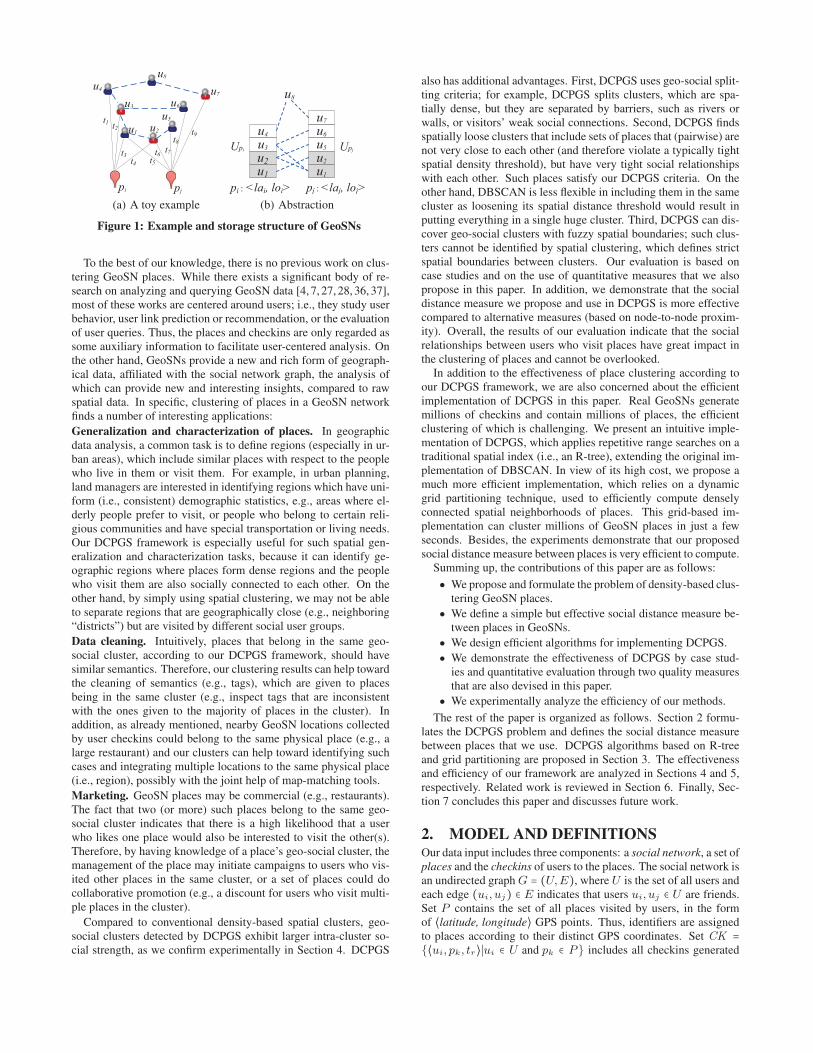
We define the new problem of Density-based Clustering Placesin Geo-Social Networks (DCPGS), to detect geo-social clusters inGeoSNs. DCPGS extends DBSCAN by replacing the Euclideandistance threshold eps for the extents of dense regions by a thresh-old ε, which considers both the spatial and the social distances be-tween places. For two places pi and pj , the spatial distance is con-sidered to be the Euclidean distance between pi and pj , while thesocial distance should consider the social relationships between thetwo sets of users Upi and Upj which have checked in pi and pj , re-spectively. We define and use such a social distance measure, basedon the intuition that two places are socially similar if they sharemany common users in their checkin records or the users in theserecords are linked by friendship edges. Figure 1(a) illustrates thedata of a GeoSN that includes eight users (u1–u8) and two places(pi and pj). The dashed lines represent user friendships and thesolid lines annotated with timestamps (t1–t9) illustrate checkins ofusers at places. For instance, user u1 is a friend with u2 and u3 andhas visited place pi at time t3 and pj at t5. As Figure 1(b) shows,each place is modeled by its spatial coordinates (e.g., ⟨lai, loi⟩ forthe latitude and longitude of pi) and the set of users that have visitedit (e.g., Upi for pi). For the spatial distance between pi and pj , wecan use the Euclidean distance between ⟨lai, loi⟩ and ⟨laj , loj⟩,while for the social distance component we use the set of com-mon users in Upi and Upj (e.g., {u1, u2}) and the users in oneplace’s record who are friends with visitors of the other place (e.g.,u3 ∈ Upi and u6 ∈ Upj who are friends with each other). Theintuition is that users who are friends can influence each other tovisit the places included in their checkin history. The details of ourdistance measure are presented in Section 2.

1http://gowalla.com2https://foursquare.com3https://www.facebook.com/about/location

u4

u8

u7

u6

u5

u2u1

u3

pjpi

t3

t1 t2

t4 t5t6 t7

t8t9

(a) A toy example

u4

u3

u2u1

u6

u5

u2

u1

u7

Upi

u8

Upj

pi : <lai, loi> pj :<laj, loj>(b) Abstraction

Figure 1: Example and storage structure of GeoSNs

To the best of our knowledge, there is no previous work on clus-tering GeoSN places. While there exists a significant body of re-search on analyzing and querying GeoSN data [4, 7, 27, 28, 36, 37],most of these works are centered around users; i.e., they study userbehavior, user link prediction or recommendation, or the evaluationof user queries. Thus, the places and checkins are only regarded assome auxiliary information to facilitate user-centered analysis. Onthe other hand, GeoSNs provide a new and rich form of geograph-ical data, affiliated with the social network graph, the analysis ofwhich can provide new and interesting insights, compared to rawspatial data. In specific, clustering of places in a GeoSN networkfinds a number of interesting applications:

Generalization and characterization of places. In geographicdata analysis, a common task is to define regions (especially in ur-ban areas), which include similar places with respect to the peoplewho live in them or visit them. For example, in urban planning,land managers are interested in identifying regions which have uni-form (i.e., consistent) demographic statistics, e.g., areas where el-derly people prefer to visit, or people who belong to certain reli-gious communities and have special transportation or living needs.Our DCPGS framework is especially useful for such spatial gen-eralization and characterization tasks, because it can identify ge-ographic regions where places form dense regions and the peoplewho visit them are also socially connected to each other. On theother hand, by simply using spatial clustering, we may not be ableto separate regions that are geographically close (e.g., neighboring“districts”) but are visited by different social user groups.

Data cleaning. Intuitively, places that belong in the same geo-social cluster, according to our DCPGS framework, should havesimilar semantics. Therefore, our clustering results can help towardthe cleaning of semantics (e.g., tags), which are given to placesbeing in the same cluster (e.g., inspect tags that are inconsistentwith the ones given to the majority of places in the cluster). Inaddition, as already mentioned, nearby GeoSN locations collectedby user checkins could belong to the same physical place (e.g., alarge restaurant) and our clusters can help toward identifying suchcases and integrating multiple locations to the same physical place(i.e., region), possibly with the joint help of map-matching tools.

Marketing. GeoSN places may be commercial (e.g., restaurants).The fact that two (or more) such places belong to the same geo-social cluster indicates that there is a high likelihood that a userwho likes one place would also be interested to visit the other(s).Therefore, by having knowledge of a place’s geo-social cluster, themanagement of the place may initiate campaigns to users who vis-ited other places in the same cluster, or a set of places could docollaborative promotion (e.g., a discount for users who visit multi-ple places in the cluster).

Compared to conventional density-based spatial clusters, geo-social clusters detected by DCPGS exhibit larger intra-cluster so-cial strength, as we confirm experimentally in Section 4. DCPGS

also has additional advantages. First, DCPGS uses geo-social split-ting criteria; for example, DCPGS splits clusters, which are spa-tially dense, but they are separated by barriers, such as rivers orwalls, or visitors’ weak social connections. Second, DCPGS findsspatially loose clusters that include sets of places that (pairwise) arenot very close to each other (and therefore violate a typically tightspatial density threshold), but have very tight social relationshipswith each other. Such places satisfy our DCPGS criteria. On theother hand, DBSCAN is less flexible in including them in the samecluster as loosening its spatial distance threshold would result inputting everything in a single huge cluster. Third, DCPGS can dis-cover geo-social clusters with fuzzy spatial boundaries; such clus-ters cannot be identified by spatial clustering, which defines strictspatial boundaries between clusters. Our evaluation is based oncase studies and on the use of quantitative measures that we alsopropose in this paper. In addition, we demonstrate that the socialdistance measure we propose and use in DCPGS is more effectivecompared to alternative measures (based on node-to-node proxim-ity). Overall, the results of our evaluation indicate that the socialrelationships between users who visit places have great impact inthe clustering of places and cannot be overlooked.

In addition to the effectiveness of place clustering according toour DCPGS framework, we are also concerned about the efficientimplementation of DCPGS in this paper. Real GeoSNs generatemillions of checkins and contain millions of places, the efficientclustering of which is challenging. We present an intuitive imple-mentation of DCPGS, which applies repetitive range searches on atraditional spatial index (i.e., an R-tree), extending the original im-plementation of DBSCAN. In view of its high cost, we propose amuch more efficient implementation, which relies on a dynamicgrid partitioning technique, used to efficiently compute denselyconnected spatial neighborhoods of places. This grid-based im-plementation can cluster millions of GeoSN places in just a fewseconds. Besides, the experiments demonstrate that our proposedsocial distance measure between places is very efficient to compute.

Summing up, the contributions of this paper are as follows:

● We propose and formulate the problem of density-based clus-tering GeoSN places.

● We define a simple but effective social distance measure be-tween places in GeoSNs.

● We design efficient algorithms for implementing DCPGS.

● We demonstrate the effectiveness of DCPGS by case stud-ies and quantitative evaluation through two quality measuresthat are also devised in this paper.

● We experimentally analyze the efficiency of our methods.

The rest of the paper is organized as follows. Section 2 formu-lates the DCPGS problem and defines the social distance measurebetween places that we use. DCPGS algorithms based on R-treeand grid partitioning are proposed in Section 3. The effectivenessand efficiency of our framework are analyzed in Sections 4 and 5,respectively. Related work is reviewed in Section 6. Finally, Sec-tion 7 concludes this paper and discusses future work.

2. MODEL AND DEFINITIONSOur data input includes three components: a social network, a set ofplaces and the checkins of users to the places. The social network isan undirected graph G = (U,E), where U is the set of all users andeach edge (ui, uj) ∈ E indicates that users ui, uj ∈ U are friends.Set P contains the set of all places visited by users, in the formof ⟨latitude, longitude⟩ GPS points. Thus, identifiers are assignedto places according to their distinct GPS coordinates. Set CK ={⟨ui, pk, tr⟩∣ui ∈ U and pk ∈ P} includes all checkins generated

by users in U . For a place pk, the set Upk of visiting users of pkis defined by Upk = {ui∣⟨ui, pk,∗⟩ ∈ CK}, where ∗ means anytime. Figure 1(b) shows Upi and Upj for the two places pi andpj of the toy example in Figure 1(a). The figure also connects theuser pairs in the two sets who are linked by friendship edges in thesocial network. Note that user u8 does not belong to either Upi orUpj , but connects users u4 and u7 in the social graph.

2.1 DCPGS ModelOur Density-based Clustering Places in Geo-Social Networks(DCPGS) model extends the model of DBSCAN [9]; for each placepi in the GeoSN, DCPGS finds the geo-social ε-neighborhoodNε(pi) of pi, which includes all places pj such that Dgs(pi, pj) ≤ε, DS(pi, pj) ≤ τ , and E(pi, pj) ≤ maxD . For two places pi,pj , E(pi, pj) is the Euclidean distance, DS(pi, pj) is the socialdistance, and Dgs(pi, pj) = f(DS(pi, pj),E(pi, pj)) is the geo-social distance, defined as a function of E(pi, pj) and DS(pi, pj).Parameter ε is geo-social distance threshold, while τ and maxDare two sanity constraints for the social and the spatial distances be-tween places, respectively. We will give detailed definitions for allabove distance functions and parameters later on. If the geo-socialε-neighborhood of a place pi contains at least MinPts places, thenpi is a core place; in this case, pi and all places in its geo-socialε-neighborhood should belong to a cluster r(pi). If another coreplace pj belongs to cluster r(pi), then r(pi) = r(pj), i.e., the clus-ters defined by pi and pj are merged. After identifying all coreplaces and merging the corresponding clusters, DCPGS ends upwith a set of (disjoint) clusters and a set of outliers (i.e., places thatdo not belong to the geo-social ε-neighborhood of any core place).In Section 3, we present algorithms for generating DCPGS clusters.

Parameters. ε and MinPts are the main parameters of DCPGS.MinPts (i.e., the minimum number of places in the neighborhoodof a core point) is set as in the original DBSCAN model (see [9]); atypical value is 5. ε takes a value between 0 and 1, because, as weexplain later on, we define Dgs(pi, pj) to take values in this range.Since the geo-social distance Dgs(pi, pj) is a function of a spatialand a social distance, τ and maxD constrain these individual dis-tances to avoid the following two cases that negatively affect thequality of geo-social clusters.

● The geo-social distance between two places pi and pj couldbe less than ε if they are extremely close to each other inspace, but have no social connection at all. This may leadto putting places close to each other spatially, but having nosocial relationship, into the same cluster.

● The geo-social distance between two places pi and pj couldbe less than ε if they have very small social distance, but theyare extremely far from each other spatially. This may leadto putting places with close social distances, but large spatialdistances, into the same cluster.

Constraints τ and maxD are defined for quality control and canbe set by experts or according to the analyst’s experience. We ex-perimentally study how clustering quality is affected by the twoconstraints and ε in Section 4.

Distance Functions. The social distance DS(pi, pj) takes as in-puts the sets of users Upi and Upj who have visited pi and pj , re-spectively, and returns a value between 0 and 1. In Section 2.2, wepresent our definition for DS(pi, pj) and alternative ways to de-fine it based on previous work. Before defining the geo-social dis-tance Dgs(pi, pj), we normalize the Euclidean distance E(pi, pj)to a spatial distance DP (pi, pj) = E(pi,pj)

maxDthat takes values be-

tween 0 and 1. Finally, Dgs(pi, pj) is defined as weighted sum of

DS(pi, pj) and DP (pi, pj), i.e.,

Dgs(pi, pj) = ω ⋅DP (pi, pj) + (1 − ω) ⋅DS(pi, pj), (1)

where ω ∈ [0,1].2.1.1 Alternatives to DCPGS

Our place clustering model (DCPGS) extends density-based clus-tering in spatial databases. GeoSN places can alternatively be clus-tered by the use of graph clustering models. The main idea ofsuch a model is to construct a place network PN , which connectsplaces according to their social and spatial distances and then applyan off-the-shelf community detection algorithm on PN . Specif-ically, given two places pi and pj , if E(pi, pj) ≤ maxD andDS(pi, pj) ≤ τ , an undirected and weighted edge with geo-socialweight Wgs(pi, pj) = 1 − Dgs(pi, pj) is added between pi andpj . Community detection algorithms like Link Clustering [1, 6] orMetis [16] can then be applied to derive the clusters. Link Clus-tering constructs a dendrogram of network communities (that mayoverlap) in a hierarchical manner. Metis is another multilevel graphpartition paradigm that includes three phases: graph coarsening,initial partitioning, and uncoarsening; Metis divides a network intok non-overlapping communities. As we will show in Section 4,these graph clustering methods are inferior to DCPGS.

2.2 Social Distance Between PlacesThe social distance DS(pi, pj) between pi and pj naturally de-pends on the social network relationships between the sets Upi andUpj of users who visited pi and pj , respectively. Our definition forDS(pi, pj) is based on the set CU ij of contributing users betweentwo places pi and pj :

Definition 1. (Contributing Users) Given two places pi and pjwith visiting users Upi and Upj , respectively, the set of contributingusers CU ij for the place pair (pi, pj) is defined as

CU ij = {ua ∈ Upi ∣ua ∈ Upj or ∃ub ∈ Upj , (ua, ub) ∈ E}∪ {ua ∈ Upj ∣ua ∈ Upi or ∃ub ∈ Upi , (ua, ub) ∈ E} (2)

Specifically, if a user ua has visited both pi and pj , then ua isa contributing user. Also if ua has visited place pi, ub has visitedpj , and ua and ub are friends, both ua and ub are contributingusers. Users in CU ij contribute positively (negatively) to the socialsimilarity (distance) between pi and pj . Formally:

Definition 2. (Social Distance) Given two places pi and pj withvisiting users Upi and Upj , respectively, the social distance be-tween pi and pj is defined as

DS(pi, pj) = 1 − ∣CU ij ∣∣Upi ∪Upj ∣ (3)

The above definition of DS(pi, pj) takes both the set similaritybetween sets Upi and Upj and the social relationships among usersin Upi and Upj into account. In addition, the distance measure pe-nalizes pairs of places pi and pj which are popular (i.e., Upi and/orUpj are large) but their set of contributing users is relatively small(see Equation 3). The reason is that such place pairs are not charac-teristic to their (loose) social connections. As an example, considerplaces pi and pj of Figure 1. To compute DS(pi, pj), we first setUpi = {u1, u2, u3, u4} and Upj = {u1, u2, u5, u6, u7}. All usersin Upi and Upj are checked one by one to obtain the contributingusers between pi and pj . We derive CU ij = {u1, u2, u3, u5, u6},since (i) both u1 and u2 have visited pi and pj , (ii) user u3, whovisited pi, has a friend u6 who visited pj , (iii) symmetrically, user

u6, who visited pj , has a friend u3 who visited pi, and (iv) u5

(∈ Upj ) has a friend u2 having been to pi. According to Definition2, the social distance DS(pi, pj) between pi and pj in Figure 1 is1 − ∣CU ij ∣/(∣Upi ∪Upj ∣) = 1 − 5/7 ≈ 0.2857.

Observe that only direct friendship edges between users of Upi

and Upj are considered in our social distance definition. Longernetwork paths, such as friend-of-friend relationships, are ignored(e.g., the case of users u4 and u7 in Figure 1(b) who are connectedvia user u8). According to the small world effect [20], a user in asocial network can reach a large portion of other users within onlyfew hops. For instance, the 90-percentile effective diameter [17] ofGowalla GeoSN, used in our experiments, is just 5.7.4 This meanswithin quite a few hops most users can reach a very large percent-age of all users. In Gowalla, only 8 users can access more than1% of all the users in 1 hop, while 40516 users (20.61% of allthe users) can access more than 1% of all the users in 2 hops and141582 users (72.02% of all the users) can reach more than 1% ofall the users in 3 hops. The number of users who can reach morethan 1% users in 2 or 3 hops increases dramatically compared tothe percentage of those visited within 1 hop. Thus, paths longerthan 1 hops are too common and cannot be considered as (indirect)user relationships; i.e., their impact is much weaker compared to di-rect friendship edges. Hence, Definition 2 introduces a simple, butpowerful social distance measure. Properties of DS(pi, pj) includesymmetry (i.e., DS(pi, pj) =DS(pj , pi)) and self-minimality (i.e.,DS(pi, pj) ∈ [0,1], and DS(pi, pj) = 0 for Upi = Upj ). On theother hand, DS(pi, pj) does not obey the triangular inequality, butthis does not affect our clustering algorithm.

2.2.1 Alternatives to DS

Our DCPGS model is independent of the social distance definitionbetween places (i.e., DS). As an alternative to our Definition 2,the following measures can be used. In Section 4, we evaluate theeffectiveness of these alternatives.

Jaccard. Based on the Jaccard similarity J(pi, pj) = (∣Upi ∩Upj ∣)/(∣Upi ∪ Upj ∣) between the sets of visiting users for pi andpj , we can define the following distance:

DJacS (pi, pj) = 1 − J(pi, pj)

DJacS (pi, pj) is not intuitive; it disregards the social network, as-

suming that two users who are friends do not affect each other invisiting GeoSN places.

SimRank. SimRank is a structural-context model for measuringthe similarity between nodes in a graph. The idea is that two nodesare equivalent if they relate to equivalent nodes. We can define aSimRank-based social distance Dsim

S (pi, pj), using the Minimaxversion of SimRank [14].5 This measure compares each of pi’svisiting users upi

r with the visiting user upjs of pj who is the most

similar to upir , to compute the similarity between places s(pi, pj).

The similarity between users s(upir , u

pjs ) is computed in an analo-

gous way. Specifically,

DsimS (pi, pj) = 1 − s(pi, pj),

where s(pi, pj) =min(spi(pi, pj), spj (pi, pj)),spi(pi, pj) = φ

∣Upi∣ ∑ur∈Upi

maxus∈Upj

s(ur, us),where φ = 0.8 is a decay factor [14],s(ur, us) = min(sur(ur, us), sus(ur, us)), and assuming that

4http://snap.stanford.edu/data/index.html5The original SimRank measure is only meant for node-to-nodesimilarity; in our case, we need a measure between Upi and Upj .

Pur is the set of places visited by ur ,sur(ur, us) = φ

∣Pur ∣∑

pi∈Pur

maxpj∈Pus

s(pi, pj).Katz. The Katz similarity measure [34] sums over all possiblepaths from user ur to us with exponential damping by length, i.e.,

K(ur, us) = ∞∑l=1

βl∣paths lur,us∣, where paths lur,us

is the set of all

length-l paths from ur to us, and damping factor β is typically setto 0.05. Due to the poor scalability of this measurement, in practiceonly paths up to length L are considered [33]; i.e., an approximated

Katz score Ka(ur, us) = L∑l=1

βl∣paths lur,us∣ can be used. Accord-

ingly, we can define a Katz-based social distance between places piand pj , by averaging the normalized Katz similarities between allpairs of users from Upi and Upj :

DKatzS (pi, pj) = 1 − 1

∣Upi ∣∣Upj ∣ ∑ur∈Upi

∑us∈Upj

Ka(ur, us)

CommuteTime. The hitting time h(ur, us) from ur to us is theexpected number of steps required for a random walk starting at ur

to reach us. The commute time between ur and us is defined byct(ur, us) = h(ur, us) + h(us, ur). However, the commute timeis sensitive to long paths and favors nodes of high degree. Thus, thetruncated commute time [26], which considers only paths of lengthno longer than L, can be used to model the social distance betweena pair of users. Finally, we can define a commute time based socialdistance between places pi and pj as follows:

DctS (pi, pj) = 1

∣Upi ∣∣Upj ∣ ∑ur∈Upi

∑us∈Upj

ctL(ur, us)

where ctL(ur, us) is the normalized truncated commute time.

3. ALGORITHMSWe propose two algorithms for DCPGS. DCPGS-R (Section 3.1)is based on the R-tree index, while DCPGS-G (Section 3.2) uses agrid partitioning.

3.1 Algorithm DCPGS-R: R-tree basedAlgorithm DCPGS-R is a direct extension of the DBSCAN algo-rithm; it uses an R-tree to facilitate the search of the geo-socialε-neighborhood for a given place. Initially, all places in the GeoSNare bulk-loaded into an R-tree. Then, DCPGS-R examines allplaces and, given a place pi, it performs a range query centeredat pi with radius maxD to get a set of candidate places that mayfall in the geo-social ε-neighborhood of pi, i.e., Nε(pi). Recallthat maxD is the maximum allowed spatial distance between placepi and places in its geo-social ε-neighborhood. Then, DCPGS-Rkeeps in Nε(pi) only the candidates that satisfy the social distanceconstraint τ and the geo-social distance threshold ε.

For the sake of efficiency, the social network is stored in a hashtable. Specifically, each pair of friends in the social network isrecorded as an entry in the hash table, such that checking whethertwo users are friends or not only incurs constant cost. In addition,for each place pi, we keep track of its visiting users Upi . The com-putation of the social distance (Definition 2) between two places piand pj involves finding the pairs of friends between sets Upi andUpj and has insignificant cost compared to the range queries usedto compute the set of candidate places.

Algorithm 1 is the pseudocode of DCPGS-R. The identity of thecurrent cluster cid is initialized to 1 in line 1. Queue Q (initializedin line 2) stores the places that have the potential to be added to the

current cluster. Hash table H records whether the geo-social dis-tances between pairs of places have been computed before (line 3)and its use will be explained later. For each unprocessed place pi,its geo-social ε-neighborhood Nε(pi) is obtained by calling func-tion GETNEIGH(pi, ε, τ , maxD , MinPts , ω, H), outlined in Al-gorithm 2. A place is unprocessed if its geo-social ε-neighborhoodhas not been computed before. If Nε(pi) contains at least MinPtsplaces, then pi is a core place, i.e., pi belongs to a cluster and allplaces in Nε(pi) should be given the same cid as pi (lines 6-11).Next, all unprocessed places in Nε(pi) are pushed into Q for laterprocessing. Lines 12-20 expand the current cluster cid as much aspossible by checking the geo-social ε-neighborhood of the unpro-cessed places in Q. No more places can be included in the currentcluster when Q is empty. In this case, the algorithm proceeds tofind the next cluster (cid is increased in line 21).

Algorithm 1 DCPGS-R(GeoSN, ε, τ , maxD , MinPts , ω)

1: cid = 12: Q = empty3: Geo-social distance cache H4: for each unprocessed place pi in GeoSN do5: Nε(pi) = GETNEIGH(pi, ε, τ , maxD , MinPts , ω, H)6: if ∣Nε(pi)∣ ≥MinPts then7: assign cid to pi8: for each place pj ∈ Nε(pi) do9: assign cid to pj

10: if pj is unprocessed then11: Q.push(pj)

12: while !Q.isEmpty() do13: pk = Q.pop()14: if pk is unprocessed then15: Nε(pk) = GETNEIGH(pk , ε, τ , maxD , MinPts , ω, H)16: if ∣Nε(pk)∣ ≥MinPts then17: for each place pm ∈ Nε(pk) do18: assign cid to pm19: if pm is unprocessed then20: Q.push(pm)

21: cid = cid + 1

Function GETNEIGH, shown in Algorithm 2, is used to get thegeo-social ε-neighborhood of place pi. Initially Nε(pi) is empty.Lines 2-4 first perform a spatial range query centered at the currentplace pi with radius maxD to get a candidate set CandSet con-taining the places that may fall in Nε(pi). If the size of CandSetis less than MinPts , Nε(pi) definitely includes less than MinPtsplaces and, therefore, pi is a non-core place. Otherwise, the al-gorithm tries to compute the social distance between every pointpj ∈ CandSet and pi. However, before this, given the fact that thespatial distance between pi and every candidate place pj is alreadyobtained in the spatial range query step, a spatial filter is employedto avoid unnecessary social distance computations (line 6).

PROPOSITION 1. Spatial filter. Given two places pi and pjwith spatial distance DP (pi, pj), if ω ⋅ DP (pi, pj) > ε, thenω ⋅DP (pi, pj) + (1 − ω) ⋅DS(pi, pj) > ε.

PROOF. Since ω ∈ [0,1] and DS(pi, pj) ∈ [0,1], (1 − ω) ⋅DS(pi, pj) ≥ 0. Consequently, if ω ⋅ DP (pi, pj) > ε, then ω ⋅DP (pi, pj) + (1 − ω) ⋅DS(pi, pj) > ε.

Note that distances Dgs and DS and DP are all symmetric.Hence, given a place pi, if pj is (not) in Nε(pi), then pi is also(not) in Nε(pj), and vice versa. Therefore, we keep track in ahash table H (line 14) whether pi and pj are in each other’s geo-social ε-neighborhood once their geo-social distance has been com-puted. This information is used when computing the geo-social ε-neighborhood of pj later (line 7-9), in order to avoid computing

the distance between the same pair of places twice. Lines 11-15compute distances, verify candidates, and update H if necessary.Line 16 is another filter, called sufficient filter, to check whetherthere are enough remaining candidate places in CandSet to renderpi’s geo-social ε-neighborhood dense. If no, the algorithm can stopwithout checking the remaining candidate places and return.

Algorithm 2 GETNEIGH(pi, ε, τ , maxD , MinPts , ω, H)

1: Nε(pi) ← ∅2: CandSet = RANGEQUERY(pi,maxD )3: if ∣CandSet ∣ <MinPts then4: return Nε(pi)

5: for each place pj ∈ CandSet do6: if ω ⋅DP (pi, pj) ≤ ε then7: if H.exists((pi, pj)) then8: if H[(pi, pj)] is TRUE then9: Nε(pi).insert(pj)

10: else11: Compute DS(pi, pj) and Dgs(pi, pj)12: if DS(pi, pj) ≤ τ && Dgs(pi, pj) ≤ ε then13: Nε(pi).insert(pj)14: H[(pi, pj)] ← TRUE15: CandSet .erase(pj)16: if ∣CandSet ∣ + ∣Nε(pi)∣ <MinPts then break17: return Nε(pi)

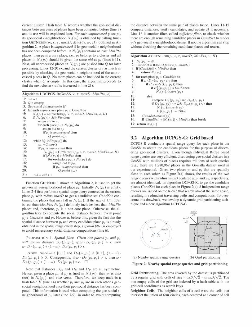
3.2 Algorithm DCPGS-G: Grid basedDCPGS-R conducts a spatial range query for each place in theGeoSN to obtain the candidate places for the purpose of discov-ering geo-social clusters. Even though individual R-tree basedrange queries are very efficient, discovering geo-social clusters in aGeoSN with millions of places requires millions of such queries(e.g., there are 1,280,969 places in the Gowalla dataset used inour experiments). Given two places pi and pj that are spatiallyclose to each other, as Figure 2(a) shows, the results of the tworange queries with radius maxD centered at pi and pj , respectively,are almost identical. In algorithm DCPGS-R, to get the candidateplaces CandSet for each place in Figure 2(a), 8 independent rangequeries are issued on the R-tree that search almost the same space,resulting in redundant traversing paths and computations. To over-come this drawback, we develop a dynamic grid partitioning tech-nique and a new algorithm DCPGS-G.

pi pj

maxDmaxD

(a) Nearby spatial range queries

2maxD

maxD

2maxD

maxD

maxD

maxD

(b) Grid partitioning

Figure 2: Nearby spatial range queries and grid partitioning

Grid Partitioning. The area covered by the dataset is partitionedby a regular grid with cells of size maxD/√2 ×maxD/√2. Thenon-empty cells of the grid are indexed by a hash table with thegrid cell coordinates as search keys.

Neighbor Cells. The neighbor cells of a cell c are the cells thatintersect the union of four circles, each centered at a corner of cell

c with radius maxD . For example, in Figure 2(b), the 20 gray cells(except c) are the neighbor cells of c, denoted as NC (c). We cantrivially show that for any place p inside c, the content of p’s geo-social ε-neighborhood is contained in NC (c) and c itself.

Cluster Discovery. Algorithm 3 is a pseudocode for DCPGS-G. Itincludes three phases. First, the algorithm maps all places into gridcells (line 1). Second, it obtains the geo-social ε-neighborhoodsof all places (lines 2-6). The third phase discovers all geo-socialclusters in the GeoSN (line 7). The geo-social ε-neighborhoods ofplaces are computed at the grid cell level. Specifically, for eachnonempty and unprocessed cell c, function GETNEIGHCELLS re-trieves its neighbor cells NC (c) (GETNEIGHCELLS is trivial andthus details are omitted). A cell is ‘unprocessed’ if its neighborcells have not been retrieved before. Function COMPCELLPAIR

(Algorithm 4) first filters out the pairs of places (pi, pj) with spa-tial distance greater than maxD , where pi ∈ c, pj ∈ NC (c) andpi ≠ pj . This step is not needed if pi and pj are in the same cell (inthis case, the spatial distance between pi and pj is certainly at mostmaxD). Next, the pairs of places (pi, pj) that satisfy the socialdistance constraint τ and the geo-social distance threshold ε are se-lected. If pi and pj are in each others’ geo-social ε-neighborhood,their corresponding Nε(pi) and Nε(pj) are updated. After all cellshave been processed, meaning that the geo-social ε-neighborhoodsof all places in the GeoSN are acquired, function GETCLUSTERS

is called to discover geo-social clusters following the frameworkof DCPGS-R (Algorithm 1), except that the Nε(pi) of each placepi has already been computed. Note that an unprocessed place piin function GETCLUSTERS means that the size of pi’s geo-socialε-neighborhood, ∣Nε(pi)∣, has not been checked.

Algorithm 3 DCPGS-G(GeoSN, ε, τ,maxD ,MinPts, ω)

1: Map all places into grid cells2: for each nonempty && unprocessed cell c do3: COMPCELLPAIR(c, c, ε, τ,maxD , ω)4: NC (c)=GETNEIGHCELLS(c)5: for each nonempty && unprocessed cell c′ ∈ NC (c) do6: COMPCELLPAIR(c, c′, ε, τ,maxD , ω)

7: GETCLUSTERS(Nε, MinPts)

Complexity. With the help of grid partitioning, the geo-social ε-neighborhood of all places in cell c can be obtained by checkingall c’s neighbor cells; the whole process can be completed within asingle pass of the data. Thus, the complexity of DCPGS-G is O(n),as each of its three phases makes one pass over the data. However,algorithm DCPGS-R computes the geo-social ε-neighborhoods ofeach place one by one. Hence its cost is O(n logn), given that theexpected cost of a single range query on the R-tree is O(logn).

Algorithm 4 COMPCELLPAIR(cell c, cell c′,ε, τ,maxD , ω)

1: for each pair (pi, pj) where pi ∈ c, pj ∈ c′, pi ≠ pj do

2: if c = c′ || E(pi, pj) ≤maxD then3: Compute DP (pi, pj)4: if ω ⋅DP (pi, pj) ≤ ε then5: Compute DS(pi, pj) and Dgs(pi, pj)6: if DS(pi, pj) ≤ τ && Dgs(pi, pj) ≤ ε then7: Nε(pi).insert(pj)8: Nε(pj).insert(pi)

4. QUALITATIVE ANALYSISThis section analyzes the quality of the geo-social clusters dis-covered by our proposed DCPGS framework. First, we compare

Algorithm 5 GETCLUSTERS(Nε, MinPts)

1: cid = 12: Q = empty3: for each unprocessed place pi in GeoSN do4: if ∣Nε(pi)∣ ≥MinPts then5: assign cid to pi6: for each place pj ∈ Nε(pi) do7: assign cid to pj8: if pj is unprocessed then9: Q.push(pj)

10: while !Q.isEmpty() do11: pk = Q.pop()12: if pk is unprocessed then13: if ∣Nε(pk)∣ ≥MinPts then14: for each place pm ∈ Nε(pk) do15: assign cid to pm16: if pm is unprocessed then17: Q.push(pm)

18: cid = cid + 1

DCPGS with the graph clustering approaches discussed in Sec-tion 2.1.1, in order to demonstrate the suitability of the density-based clustering model for this application. Second, we comparewith two extreme versions of DCPGS: PureSocialDistance appliesdensity-based clustering by using the social distance DS(pi, pj)only, while DBSCAN uses only the Euclidean distance E(pi, pj).This comparison shows the appropriateness of using both socialand spatial distances in clustering. In the implementation of Pure-SocialDistance, we do not put place pairs with spatial distancemore than 1000m in the same cluster; otherwise this method be-comes too expensive. Finally, we assess the suitability of our socialdistance measure (Section 2.2) by evaluating versions of DCPGS,which use the alternative social distance definitions discussed inSection 2.2.1. All tested methods were implemented in C++ andthe experiments were performed on a 3.4 GHz quad-core machinerunning Ubuntu 12.04 with 16 GBytes memory.

Data. We use two publicly available datasets6 from historicalgeo-social networks. Gowalla contains a social network with∣U ∣ =196,591 users and ∣E∣ =950,327 undirected friendship edges.There are ∣CK ∣ =6,442,892 checkins performed by those userson ∣P ∣ =1,280,969 places over a period from Feb. 2009 toOct. 2010. Brightkite includes a social network of ∣U ∣ =58,228users and ∣E∣ =214,078 undirected friendship edges. It contains∣CK ∣ =4,491,143 checkins on ∣P ∣ =772,783 distinct places col-lected over the period from Apr. 2008 to Oct. 2010.

Default Parameter Settings. The density requirement of the clus-tering is determined by parameters MinPts and ε (or DBSCAN’seps). We set MinPts = 5 for all approaches; various density set-tings can be achieved by just tuning ε (or DBSCAN’s eps). Forinstance, a large MinPts has similar effect as a small ε (or DB-SCAN’s eps). By default, parameter ω in the geo-social distanceis set to 0.5 to equally weigh the social and spatial distances. Bydefault, parameter τ is set to 0.7, and maxD is set to 100m fordataset Gowalla and 120m for dataset Brightkite.

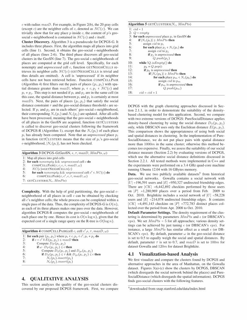
4.1 Visualization-based AnalysisWe first visualize and compare the clusters found by DCPGS andalternative approaches in the area of Manhattan, on the Gowalladataset. Figures 3(a)-(c) show the clusters by DCPGS, DBSCAN(which disregards the social network behind the places) and Pure-SocialDistance (which disregards the spatial information). DCPGSfinds geo-social clusters with the following features.

6downloaded from snap.stanford.edu/data/index.html

(a) DCPGS: ε = 0.4, τ = 0.7,maxD = 100m

′

′

(b) DBSCAN: eps = 40m (c) PureSocialDistance: ε = 0.2,τ = 1, maxD = 1000m

(d) LinkClustering: τ = 0.7,maxD = 100m

A

CB

(e) Jaccard: ε = 0.4, τ = 0.7,maxD = 100m

A

CB

(f) SimRank: ε = 0.3, τ = 0.7,maxD = 100m

Figure 3: Place clusters of Gowalla found in Manhattan

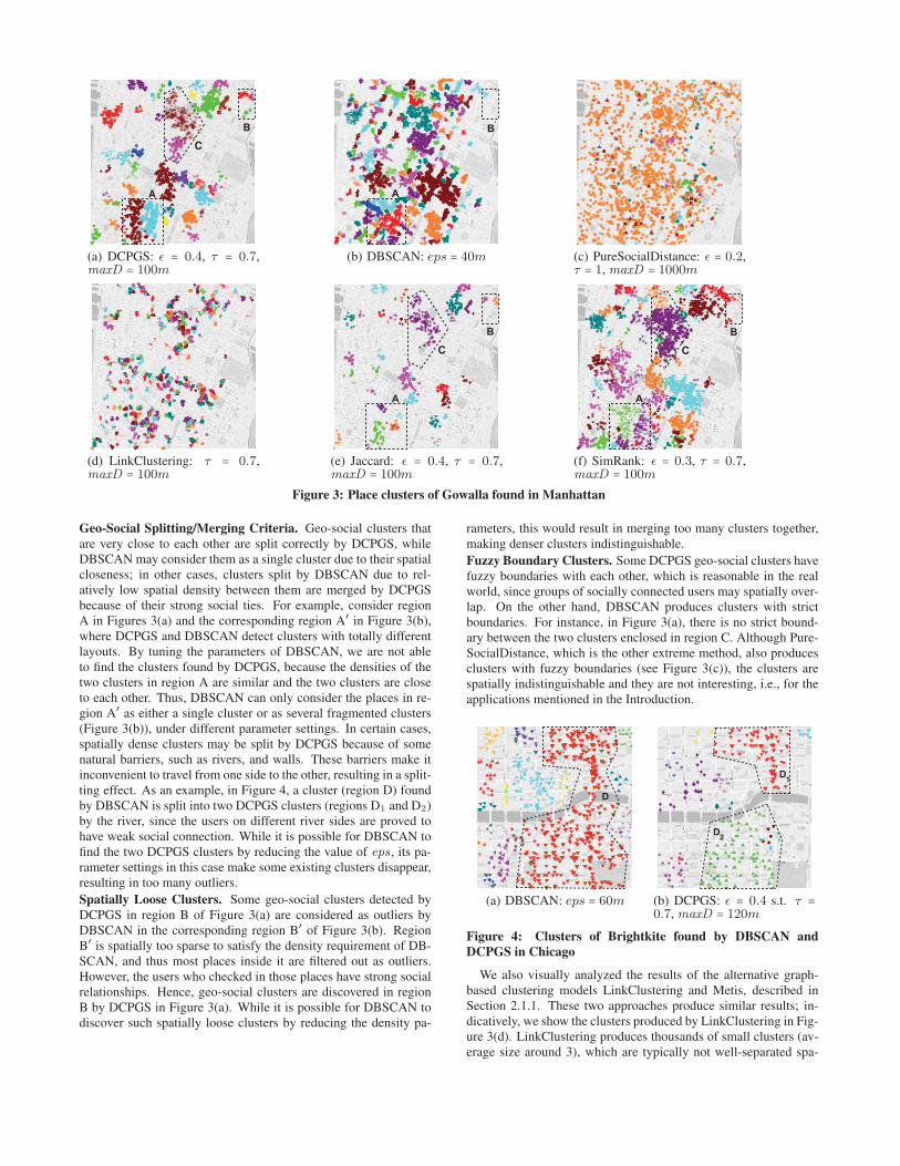
Geo-Social Splitting/Merging Criteria. Geo-social clusters thatare very close to each other are split correctly by DCPGS, whileDBSCAN may consider them as a single cluster due to their spatialcloseness; in other cases, clusters split by DBSCAN due to rel-atively low spatial density between them are merged by DCPGSbecause of their strong social ties. For example, consider regionA in Figures 3(a) and the corresponding region A′ in Figure 3(b),where DCPGS and DBSCAN detect clusters with totally differentlayouts. By tuning the parameters of DBSCAN, we are not ableto find the clusters found by DCPGS, because the densities of thetwo clusters in region A are similar and the two clusters are closeto each other. Thus, DBSCAN can only consider the places in re-gion A′ as either a single cluster or as several fragmented clusters(Figure 3(b)), under different parameter settings. In certain cases,spatially dense clusters may be split by DCPGS because of somenatural barriers, such as rivers, and walls. These barriers make itinconvenient to travel from one side to the other, resulting in a split-ting effect. As an example, in Figure 4, a cluster (region D) foundby DBSCAN is split into two DCPGS clusters (regions D1 and D2)by the river, since the users on different river sides are proved tohave weak social connection. While it is possible for DBSCAN tofind the two DCPGS clusters by reducing the value of eps , its pa-rameter settings in this case make some existing clusters disappear,resulting in too many outliers.

Spatially Loose Clusters. Some geo-social clusters detected byDCPGS in region B of Figure 3(a) are considered as outliers byDBSCAN in the corresponding region B′ of Figure 3(b). RegionB′ is spatially too sparse to satisfy the density requirement of DB-SCAN, and thus most places inside it are filtered out as outliers.However, the users who checked in those places have strong socialrelationships. Hence, geo-social clusters are discovered in regionB by DCPGS in Figure 3(a). While it is possible for DBSCAN todiscover such spatially loose clusters by reducing the density pa-

rameters, this would result in merging too many clusters together,making denser clusters indistinguishable.

Fuzzy Boundary Clusters. Some DCPGS geo-social clusters havefuzzy boundaries with each other, which is reasonable in the realworld, since groups of socially connected users may spatially over-lap. On the other hand, DBSCAN produces clusters with strictboundaries. For instance, in Figure 3(a), there is no strict bound-ary between the two clusters enclosed in region C. Although Pure-SocialDistance, which is the other extreme method, also producesclusters with fuzzy boundaries (see Figure 3(c)), the clusters arespatially indistinguishable and they are not interesting, i.e., for theapplications mentioned in the Introduction.

(a) DBSCAN: eps = 60m (b) DCPGS: ε = 0.4 s.t. τ =0.7, maxD = 120m

Figure 4: Clusters of Brightkite found by DBSCAN andDCPGS in Chicago

We also visually analyzed the results of the alternative graph-based clustering models LinkClustering and Metis, described inSection 2.1.1. These two approaches produce similar results; in-dicatively, we show the clusters produced by LinkClustering in Fig-ure 3(d). LinkClustering produces thousands of small clusters (av-erage size around 3), which are typically not well-separated spa-

tially. Due to the sparsity of geo-social network data, the con-structed place network contains many connected components thatare disconnected with each other (e.g., the place network built whenτ = 0.7, maxD = 100, and ω = 0.5 contains 34,496 connectedcomponents with 4.3 nodes and 8.2 edges on average. The clustersfound by Metis are fewer and larger, but also spatially indistin-guishable. Metis ignores outliers; as a result, places belong to thesame cluster may have low spatial proximity and social similarity.

Finally, we analyzed the results of DCPGS, if our DS definition(Definition 2) is replaced by the alternatives described in Section2.2.1. For DKatz

S and DctS , we set L = 3; for bigger L values, these

measures become extremely expensive. We observed that DJacS ,

DKatzS , and Dct

S produce similar results to each other. Indicatively,Figure 3(e) shows the clusters found by DCPGS if DJac

S is usedinstead of DS . All these measures produce small clusters and toomany outliers since they give large distance values for most pairsof places pi and pj . The set of common users for two places in Jac-card (i.e., Upi ∩ Upj ) is expected to be small and the decay factorof Katz dampens the effect of long connections between Upi andUpj . The expected CommuteTime distance between places is also

high due to the effect of normalization. On the other hand, DsimS

produces clusters of slightly larger sizes compared to DS . We ob-served that the probability distribution of Dsim

S is skewed towardslow values, meaning that many pairs of places have low bipartiteminimax SimRank social distance, because SimRank is based onthe most similar pair of visiting users. The clustering results ofSimRank (Figure 3(f)) and DCPGS are visually similar; it is hardto tell which results are better based on visualization.

4.2 Social Quality EvaluationIn this section, we design and use two measures for assessing thesocial coherence between places in the discovered clusters. Basedon these measures, we assess the quality of DCPGS and the alter-native approaches for clustering GeoSN places.

4.2.1 Social Entropy based EvaluationThe first measure, called social entropy, measures the social qualityof the clusters based on the network communities that the GeoSNusers form. Given a social network G = (U,E), we first partitionall the users in U into several disjoint network communities. LetPC be a cluster of GeoSN places. According to the detected net-work communities, the visiting users of PC , i.e., ∪p∈PCUp, canbe divided into several disjoint sets in CPC = {C1,C2, . . . ,Cm},such that each set Ci is a subset of users in CPC belonging to thesame network community. We call CPC the community set of PC .

Definition 3. (Social Entropy) Given a cluster PC , let UPC bethe set of users who visit the places in PC , i.e., UPC = ∪p∈PCUp.The social entropy of PC is then defined as:

E = ∑Ci∈CPC

− ∣Ci∣∣UPC ∣ log

∣Ci∣∣UPC ∣

The social entropy, analogous to the entropy used in decision treeinduction, measures the impurity of a cluster PC with respect to theparticipation of its users into different communities. A low socialentropy means that the great majority of the visitors of PC comefrom the same community (i.e., low impurity), indicating that theplaces in PC have tighter social relationships between each other,which is favored.

We applied the METIS community detection algorithm [16] todivide the set of users in the GeoSN into k non-overlapping com-

munities7, providing a baseline for social entropy evaluation. Toavoid a comparison that is biased to parameter k, we evaluate thesocial entropy of clustering results obtained by DCPGS and thecompetitors for two different values of k. One value of k is cho-

sen based on the following rule of the thumb [19], i.e., k = √N/2where N is the number of users in the social network. The othervalue of k is decided by Dunbar’s number that suggests humans canonly comfortably maintain 150 stable relationships and the meancommunity size is around 150. For dataset Gowalla, these valuesare k = 313 and k = 1310, respectively.

Figures 5(a) and 5(b) show the average social entropy forDCPGS, versions of DCPGS with alternative DS (SimRank, Com-muteTime, Katz, and Jaccard) and PureSocialDistance when vary-ing ε. CommuteTime, and Katz have the lowest social entropy;however, these methods produce small clusters and have too manyoutliers as explained in Section 4.1. Within each small cluster, theplaces are only visited by few people and this explains the low en-tropy. Jaccard also has low social entropy for the same reason.PureSocialDistance has low social entropy in most cases; this indi-cates that our proposed social distance between places is effectivein putting places with close social relationships together. Whenε = 0.1, the social entropies of DCPGS and PureSocialDistance aresimilar, both good, since only those places with very close socialdistances are clustered. When ε = 1, PureSocialDistance has no so-cial distance constraint τ thus its entropy becomes higher than thatof DCPGS. DCPGS outperforms SimRank-based DCPGS, mean-ing that our proposed social distance is better than the SimRank-based Dsim

S (pi, pj) distance. When k = 1310, the average socialentropy of all the methods is larger than in the case where k = 313,since a larger number of network communities increases the prob-ability that users in a single cluster belong to diverse communities.The average cluster size increases with ε, increasing the probabilitythat the visitors of a cluster belong to different communities; thus,the average social entropy increases. In addition, the clusteringresult becomes stable at large values of ε, thus the social entropyconverges. By visualization, we observed that ε should be set to avalue smaller than 0.5 for the clustering results to be interesting.

Figures 5(c) and 5(d) show the average social entropies ofDCPGS, DCPGS based on SimRank, CommuteTime, Katz, andJaccard, and the graph-based clustering methods Metis andLinkClustering, when varying the social distance constraint τ .Similar to the case when ε varies, the social entropy increasesand then stabilizes as τ increases, except for the entropy of Metis,which keeps increasing due to the network partitioning method-ology of Metis with the increase of τ , the constructed place net-work becomes less connected, however, due to its partitioning na-ture, Metis puts disconnected places in the constructed place net-work into same cluster. When τ is less than 0.5, the social entropyof CommuteTime is zero, since with these distance measures theplaces in each cluster are visited by only one person when τ < 0.5.Jaccard has low social entropy also due to the small sizes of its clus-ters. For τ ≤ 0.1 SimRank-based DCPGS fails to find any clusters,therefore the entropy is 0. After investigation, we found that thereis no pair of places pi, pj with Dsim

S (pi, pj) < 0.2 because of thedecay factor φ. When τ = 0.2, SimRank has a low social entropy,since only few (987) clusters of small size are found compared tothe 3605 clusters discovered by DCPGS. After the point where thetwo approaches find a similar number of clusters (e.g., at τ = 0.5,SimRank finds 5880 clusters, while DCPGS finds 6742 clusters),DCPGS has constantly lower entropy than SimRank. In addition,

7This is different from Metis used as a competitor of DCPGS inGeoSN place clustering (discussed in Section 2.1.1).

△ DCPGS ▽ DBSCAN ▼ PureSocialDistance☆ Jaccard × SimRank ◻ Katz● CommuteTime ∎ LinkClustering ▷ Metis

0.1 0.2 0.3 0.4 0.5 0.6 0.7 0.8 0.9 10

0.5

1

1.5

2

2.5

ε

Soc

ial E

ntro

py

(a) k = 3130.1 0.2 0.3 0.4 0.5 0.6 0.7 0.8 0.9 10

0.5

1

1.5

2

2.5

εS

ocia

l Ent

ropy

(b) k = 1310

0 0.1 0.2 0.3 0.4 0.5 0.6 0.7 0.8 0.9 10

0.5

1

1.5

2

2.5

3

3.5

4

τ

Soc

ial E

ntro

py

(c) k = 3130 0.1 0.2 0.3 0.4 0.5 0.6 0.7 0.8 0.9 1

0

0.5

1

1.5

2

2.5

3

3.5

4

τ

Soc

ial E

ntro

py

(d) k = 1310

10 50 100 150 200 250 30000.5

11.5

22.5

33.5

(DBSCAN) or (others)

Soc

ial E

ntro

py

meps maxD

(e) k = 31310 50 100 150 200 250 3000

0.51

1.52

2.53

3.54

(DBSCAN) or (others)

Soc

ial E

ntro

py

mmaxDeps

(f) k = 1310Figure 5: Social entropy evaluation in Gowalla

DCPGS is less sensitive to τ compared to SimRank. DCPGS out-performs the two graph-based competitors Metis and LinkCluster-ing. As we observed by visualization, in practice τ should be setto a value higher than 0.5, because a very tight social distance con-straint creates too few and too small geo-social clusters.

Figures 5(e) and 5(f) show the average social entropies of thevarious versions of DCPGS and all the competitor approacheswhen varying the spatial distance constraint maxD (eps for DB-SCAN). DCPGS is superior to SimRank-based DCPGS, DBSCAN,LinkClustering and Metis for all values of maxD (eps). In gen-eral, the social entropies of all methods are not very sensitive tomaxD . For Gowalla, a good value for maxD is around 100m;large maxD values result in clusters that are spatially too loose.

4.2.2 Community Score based EvaluationGiven a GeoSN place cluster PC , let UPC be the set of userswho visit the places in PC , i.e., UPC = ∪p∈PCUp. Assume eachUPC is a community in the GeoSN. We adopt the eight networkcommunity multi-criterion scores surveyed in [18] to compute thecommunity score of UPC for each cluster PC . Figure 6 com-pares the results of DCPGS and its alternatives on Gowalla (Katzis omitted because its result is quite similar to that of Commute-Time), in terms of the internal density and conductance scores. Wegroup the clusters discovered by each method by size and com-pute and plot the average community score (i.e., internal densityand conductance) for each cluster size group. The results basedon the other six criteria of [18] are similar and we omit them

due to lack of space. The internal density of UPC is defined by1 −mUPC /(∣UPC ∣(∣UPC ∣ − 1)/2), where mUPC is the number ofedges in UPC , mUPC = ∣{(u, v)∣u ∈ UPC , v ∈ UPC}∣. Conduc-tance is the fraction of edges from nodes of UPC that point outsideUPC , i.e., oUPC /(2mUPC + oUPC ), where oUPC = ∣{(u, v)∣u ∈UPC , v ∉ UPC}∣. Let f(UPC ) be the community score of PC ,based on either internal density or conductance; a smaller value off(UPC ) indicates better social quality.

As Figures 6(a) and 6(c) show, the internal density increases withthe cluster size. As the size of a place cluster increases, the de-nominator of the internal density formula increases quadraticallywhile the number of social links between users in the cluster (i.e.,the numerator) does not increase at the same pace. On the otherhand, Figures 6(b) and 6(d) show that conductance initially de-creases as the size of a cluster increases and fluctuates randomlyfor larger UPC sizes, which is in line with the observations in [18].In Figure 6, we observe that the geo-social clusters discovered byDCPGS have better community scores (i.e., lower internal densityand conductance scores) compared to all competitors, except Pure-SocialDistance. Since PureSocialDistance uses our social distancein clustering and disregards spatial proximity, its social quality isexpected to be better than that of DCPGS; still, as shown in Fig-ure 3(c), its clusters are not distinguishable spatially. DCPGS out-performs DBSCAN and SimRank-based DCPGS. The quality gapbetween DCPGS and the 3 competitors in Figure 6(a) and 6(b) nar-rows as the size of clusters increases, since it is more difficult fora larger UPC (usually obtained from a larger PC ) to maintain acommunity-like structure compared to a smaller UPC [18]. Thisindicates that our social distance is effective in finding geo-socialclusters with small or medium size. DCPGS is also generally betterthan the four competitors in Figures 6(c) and 6(d). CommuteTimehas better community scores when the cluster size is around 50.Most community scores of Jaccard, CommuteTime, LinkCluster-ing, and Metis concentrate at the top-left corner of Figures 6(c) and6(d), which indicates that these competitors have limited abilityto discover geo-social clusters of various sizes. Furthermore, thequality gap between DCPGS and the five competitors in Figures6(c) and 6(d) grows when the cluster size increases. We concludethat DCPGS (paired with our social distance measure) is the mosteffective method in finding geo-social clusters with both good so-cial quality and identifiable spatial contour.

5. EFFICIENCY EVALUATIONIn this section, we investigate the efficiency and scalability ofDCPGS and its competitors. In Section 3, we presented two al-ternative implementations of DCPGS, an R-tree based (DCPGS-R) and a grid-based (DCPGS-G). We also implemented the corre-sponding R-tree based and grid-based versions of DBSCAN, andDCPGS based on Jaccard, SimRank, Katz, and CommuteTime.Linkclustering and Metis are also compared with DCPGS. In ourcomparison, we do not include PureSocialDistance, because thismethod is too slow (it takes roughly 1 day to finish) and it is notappropriate for spatial clustering.Effect of data size. In the first experiment, we test the scalabil-ity of all methods. For this purpose, we use subsets of the twoGeoSN datasets, Gowalla and Brightkite, of various sizes. The sub-sets are determined by continuous spatial ranges, which contain thedesired cardinality of places. All place subsets are associated withthe original social network data. Five subsets with 200K, 400K,600K, 800K, and 1000K places are obtained from Gowalla. Sim-ilarly, five subsets of sizes 200K, 300K, 400K, 500K, and 600Kare extracted from Brightkite. When varying the data size, we keepε = 0.4, maxD = 100m, τ = 0.7 and ω = 0.5 for all methods in

0 50 100 150 200 250 300 350 4000.55

0.6

0.65

0.7

0.75

0.8

0.85

0.9

0.95

1

Cluster size

Inte

rnal

dens

ity

PureSocialDistanceDBSCANSimRankDCPGS

(a) Internal Density

0 50 100 150 200 250 300 350 4000.75

0.8

0.85

0.9

0.95

1

Cluster size

Cond

uctan

ce

PureSocialDistanceDBSCANSimRankDCPGS

(b) Conductance

0 50 100 150 200 250 300 350 4000.55

0.6

0.65

0.7

0.75

0.8

0.85

0.9

0.95

1

Inte

rnal

dens

ity

Cluster size

MetisLinkClusteringCommuteTimeJaccardDCPGS

(c) Internal Density

0 50 100 150 200 250 300 350 4000.75

0.8

0.85

0.9

0.95

1

Cond

ucta

nce

Cluster size

MetisLinkClusteringCommuteTimeJaccardDCPGS

(d) Conductance

Figure 6: Community score evaluation in Gowalla

Gowalla and ε = 0.4, maxD = 120m, τ = 0.7 and ω = 0.5 for allmethods in Brightkite. (LinkClustering and Metis have no ε param-eter.) Figures 7(a) and 7(b) display the runtime of all tested meth-ods. DCPGS-G is much faster than DCPGS-R and maintains itsperformance gap as the database size grows. In all cases, DCPGS-G (DCPGS-R) is only a bit slower than DBSCAN-G (DBSCAN-R) and Jaccard-G (Jaccard-R)8, while DCPGS has much highereffectiveness as shown in Section 4. SimRank-G, (SimRank-R),Katz-G, and CommuteTime-G are much slower than DBSCAN-G (DBSCAN-R). This indicates that the time overhead imposedby DCPGS over the pure-spatial DBSCAN clustering algorithmis low, proving that our effective social distance is also efficientto compute. The costs of SimRank, Katz, and CommuteTime areall dominated by the expensive Dsim

S (pi, pj), DKatzS (pi, pj), and

DctS (pi, pj) computations; optimizing their spatial search compo-

nent (i.e., replacing the R-tree search by a grid-based search) haslittle effect on their overall performance.9 Metis has similar cost toDCPGS-G, while LinkClustering is slower; these methods are noteffective for geo-social place clustering as discussed in Section 4.

Effect of ε. Figures 7(c) and 7(d) show the performance of allmethods when varying ε, except LinkClustering and Metis, whichdo not use parameter ε. We keep τ = 0.7 and ω = 0.5 for bothdatasets and maxD = 100m for Gowalla and maxD = 120mfor Brightkite. Note that DCPGS-G is faster than DCPGS-R in allcases, which again indicates that grid partitioning greatly improvesthe efficiency of DCPGS. DCPGS-G (DCPGS-R) is slightly moreexpensive than Jaccard-G (Jaccard-R). The runtimes of SimRank-G, SimRank-R, Katz-G, and CommuteTime-G increase signifi-cantly when ε increases from 0.1 to 0.5, because the increaseweakens the power of the spatial filter (Proposition 1) and more(expensive) social distances (Dsim

S (pi, pj), DKatzS (pi, pj), and

DctS (pi, pj)) are computed. DCPGS-G and DCPGS-R remain

8To make the plots clearer, we omit the runtime of Jaccard-G(Jaccard-R) from some of them; the time of Jaccard-G (Jaccard-R) always falls between the time of DCPGS-G (DCPGS-R) andDBSCAN-G (DBSCAN-R).9This is the reason why we omit the runtimes of Katz-R andCommuteTime-R from the comparison.

▷ DCPGS-G * DCPGS-R ◁ Katz-G+ DBSCAN-G ◻ DBSCAN-R ☆ CommuteTime-G▽ SimRank-G × SimRank-R ∎ Jaccard-G� LinkClustering ● Metis ▲ Jaccard-R

2.0 4.0 6.0 8.0 10.0 12.0 14.010−1

100

101

102

103

104

105

Data size: # of places ( × 105)

Run

time

( sec

onds

)

(a) Gowalla

2.0 3.0 4.0 5.0 6.0 7.0 8.010−1

100

101

102

Data size: # of places ( × 105)

Run

time

( sec

onds

)

(b) Brightkite

0.1 0.2 0.3 0.4 0.5 0.6 0.7 0.8 0.9 1100

101

102

103

104

105

ε

Run

time

( sec

onds

)(c) Gowalla

0.1 0.2 0.3 0.4 0.5 0.6 0.7 0.8 0.9 1100

101

102

ε

Run

time

( sec

onds

)

(d) Brightkite

10 50 100 150 200 250 300100

101

102

103

104

105

Run

time

( sec

onds

)

(DBSCAN) or (others)eps maxDm

(e) Gowalla

10 50 100 150 200 250 300100

101

102

103

Run

time

( sec

onds

)

(DBSCAN) or (others)eps maxDm

(f) Brightkite

0 0.1 0.2 0.3 0.4 0.5 0.6 0.7 0.8 0.9 1101

102

103

104

105

ω

Run

time

( sec

onds

)

(g) Gowalla

0 0.1 0.2 0.3 0.4 0.5 0.6 0.7 0.8 0.9 1100

101

102

ω

Run

time

( sec

onds

)

(h) Brightkite

Figure 7: Runtime experiments

quite stable for all ε values since the computational cost of our so-cial distance is insignificant.

Effect of maxD (eps in DBSCAN). Parameter maxD (eps in DB-SCAN) decides the spatial ranges of the geo-social (spatial) neigh-borhoods of places and the size of the constructed place network forLinkClustering and Metis. Thus, maxD (eps) greatly influencesthe efficiency of all methods. Figures 7(e) and 7(f) display the run-time of all methods when varying maxD (eps). We set τ = 0.7,ε = 0.4, and ω = 0.5 for all the methods except DBSCAN on bothGowalla and Brightkite datasets. Note that SimRank-G, SimRank-R, Katz-G and CommuteTime-G are more sensitive to maxD com-pared to the other methods, due to the high cost of Dsim

S (pi, pj),DKatz

S (pi, pj), and DctS (pi, pj) distance computations. The cost

of DCPGS-G stays below 100 seconds as maxD ranges from 10mto 300m and remains close to that of DBSCAN-G and Jaccard-G.DCPGS-R is also close to DBSCAN-R and Jaccard-R. DCPGS-G remains faster than DCPGS-R, but their performance gap nar-rows with maxD ; the reason is that grid-based computations be-come more expensive as the grid cell size (i.e., maxD) increases.DCPGS-R eventually becomes faster than DCPGS-G for a verylarge maxD , e.g. maxD > 1000m; however, as shown in Fig-ure 3(c), geo-social clusters with a very large maxD are not spa-tially identifiable. At an appropriate maxD value (around 100m),DCPGS-G is clearly the best choice. Metis has similar cost toDCPGS-G while LinkClustering is slower.

Effect of ω. Figures 7(g) and 7(h) display the runtimes of the clus-tering methods when varying ω. We keep τ = 0.7 and ε = 0.4 for allmethods on both datasets, while setting maxD = 100m in Gowallaand maxD = 120m in Brightkite. The costs of all methods are notmuch sensitive to ω; an exception is the runtimes of SimRank-G,SimRank-R, Katz-G, and CommuteTime-G which decrease whenω > 0.5. The reason is again the high effect of the spatial filter(Proposition 1), when ω is large, due to which many expensive so-cial distance computations are avoided. As a final note, the socialdistance constraint τ is only applied as an ultimate filter and has noinfluence on the runtimes of all methods. It only slightly influencesthe costs of LinkClustering and Metis because it affects the size ofthe place network, on which these methods operate.

6. RELATED WORKOur clustering problem is related to various research topics, in-cluding traditional spatial clustering, using mobility data to analyzeplaces, clustering using spatial and non-spatial attributes, studyingthe relationship between spatial and social attributes, communitydetection, and other work on GeoSNs.

Spatial Clustering. Spatial clustering algorithms, surveyed in[12], are divided into three categories: partitioning, hierarchi-cal and density-based clustering. Partitioning methods, includ-ing k-means, k-medoids, and CLARANS [23], are good at find-ing spherical-shaped clusters in small and medium-sized datasets.They need a pre-defined parameter k to specify the number ofclusters obtained. However, partitioning methods are not able todetect clusters of arbitrary shapes. Hierarchical clustering tech-niques, such as BIRCH [41], Chameleon [15] and CURE [11], as-sign objects to clusters in two fashions: agglomerative (bottom-up)and divisive (top-down). Hierarchical clustering methods do nothave well-defined termination criteria and cannot correct the re-sult if some objects are assigned to the wrong clusters at an earlystage. Density-based clustering methods, like DBSCAN [9], dis-cover clusters of arbitrary shapes and sizes. Objects in dense re-gions are grouped as clusters, while objects in sparse regions are la-beled as outliers. OPTICS [3] is an extension of DBSCAN, whichgenerates an augmented ordering of the dataset that captures itsdensity-based clustering structure at different granularities. DEN-CLUE [13] models the overall point density analytically as thesum of influence functions of the data points. Clusters can thenbe identified by determining density-attractors and clusters of ar-bitrary shapes can be easily described by a simple equation basedon the overall density function. GDBSCAN [25] is a generaliza-tion of DBSCAN that clusters point objects as well as spatially ex-tended objects according to both their spatial and their non-spatialattributes. Our work adopts the density-based clustering frameworkto find place clusters in a geo-social network, by considering boththe spatial distance and the social coherence of the places.

Analysis of Places based on Mobility Data. Brilhante et al. [6]detect “communities” of places of interest (POIs) on a map basedon how strongly the places are correlated in sequences of visitsby mobile users. Different from our work, the social relationshipsbetween the users who visit the places and the spatial distances be-tween places are disregarded. The co-existence of places in the vis-iting histories of users is the only criterion used for clustering. Theproposed solution generates a graph G that connects pairs POIs ac-cording to the nature of their co-existence in sequences of user vis-its and then employs a classic algorithm for community detectionon G to identify the place communities. Andrienko et al. [2] presentan analysis and visualization tool, which first identifies interestingevents of moving objects (e.g., instances of slow car movements),then spatially clusters these events, using density-based clusteringto derive a set of significant places (e.g., regions where traffic jamsoccur), and finally applies visual analytics to aggregate and ana-lyze the events with respect to parameters such as location, timeand direction of movement.

Clustering based on Spatial and Non-Spatial Attributes. Clus-tering objects based on spatial and non-spatial attributes finds ap-plications in different areas, such as computer vision, GIS, and so-cial networks. Yu et al. [39] cluster pixels considering both theRGB color vectors and spatial proximity that is useful in naturalimage segmentation. Gennip et al. [32] use spectral clustering toidentify communities in a graph where nodes are gang membersand weighted edges indicate the gang members’ social interactionsand geographic locations. Zhang et al. [40] apply clustering by ad-justing the spatial distance between two objects according to thenon-spatial attribute values between them.

Spatial-Social Relationship. The relationship between geographyand social structure has been long studied by sociologists. Re-searchers have found that the likelihood of friendship with a per-son is decreasing with distance, which has been observed withincolleges [29], new housing developments [10], and projects for theelderly [21]. Scellato et al. [27] performed a quantitative studyon the socio-spatial properties of users in GeoSNs. By utilizingsocial and spatial properties of GeoSNs, the same research groupproposed a link prediction model [28]. Ye et al. [37] designed alocation recommendation system in the context of GeoSNs. Back-strom et al. [5] predict the location of an individual from a sparse setof known user locations using the relationship between geographyand friendship. Wang et al. [34] find that the similarity between themovements of two individuals strongly correlates with their prox-imity in the social network. This correlation is used as a tool forlink prediction in a social network. Pham et al. [24] propose anentropy-based model (EBM) that not only infers social connectionsbut also estimates the strength of social connections by analyzingpeople’s co-occurrences in space and time. Different from exist-ing work, we neither study the spatial-social relationship nor doprediction or recommendation utilizing this relationship. We per-form density-based clustering of GeoSN places considering boththe spatial distances between them and the social relationships be-tween users that visit the places.

Detecting and Evaluating Communities in Networks. There aremany existing works on network community detection and cluster-ing of nodes in a graph using only the network distance betweennodes [8, 22, 31, 35, 38]. SCAN [35] is an algorithm that detectsclusters, hubs, and outliers in networks. [38] proposed partition-ing, hierarchical and density-based algorithms to cluster objects onspatial networks, based on shortest-path distance. [18] summarizedand empirically evaluated algorithms for network community de-tection. In Section 4.2.2, we have used network community quality

measures [18] to evaluate the social quality of the place clustersfound by our algorithms.

Orthogonal Works in GeoSNs. Cho et al. [7] studied the problemof using social relationships to explain human movement. Yanget al. [36] introduced a Socio-Spatial Group Query (SSGQ) that re-trieves a group of users who have certain social connection strengthand the sum of their spatial distances is minimized. Most recently,a general framework for Geo-Social query processing that supportsRange Friends (RF), Nearest Friends (NF), and Nearest Star Group(NSG) queries was proposed in [4].

7. CONCLUSIONIn this paper, we studied for the first time the problem of Density-based Clustering Places in Geo-Social Networks (DCPGS). Ourclustering model extends the density-based clustering paradigm toconsider both the spatial and social distances between places. Wedefined a new measure for the social distance between places, con-sidering the social ties between users that visit them. Our measureis shown to be more effective and efficient to compute, comparedmore complex ones based on node-to-node graph proximity. Weanalyzed the effectiveness of DCPGS via case studies and demon-strated that DCPGS can discover clusters with interesting proper-ties (i.e., barrier-based splitting, spatially loose clusters, clusterswith fuzzy boundaries), which cannot be found by merely usingspatial clustering. Besides, we designed two evaluation measuresto quantitatively evaluate the social quality of clusters detectedby DCPGS or competitors, called social entropy and communityscore, which also confirm that DCPGS is more effective than alter-native approaches. Finally, we optimized the efficiency of DCPGSclustering with the help of a grid-based data structure. Our opti-mized DCPGS algorithm can cluster millions of places within justa few seconds. In the future, we plan to consider the influence ofthe time-span of user visits to places and the multiplicity of uservisits to a place to cluster places.

8. REFERENCES[1] Y.-Y. Ahn, J. P. Bagrow, and S. Lehmann. Link communities reveal

multiscale complexity in networks. Nature, 466:761–764, 2010.

[2] G. L. Andrienko, N. V. Andrienko, C. Hurter, S. Rinzivillo, andS. Wrobel. Scalable analysis of movement data for extracting andexploring significant places. IEEE TVCG, 19(7):1078–1094, 2013.

[3] M. Ankerst, M. M. Breunig, H.-P. Kriegel, and J. Sander. Optics:Ordering points to identify the clustering structure. In SIGMOD,1999.

[4] N. Armenatzoglou, S. Papadopoulos, and D. Papadias. A generalframework for geo-social query processing. PVLDB, 6(10):913–924,2013.

[5] L. Backstrom, E. Sun, and C. Marlow. Find me if you can:Improving geographical prediction with social and spatial proximity.In WWW, 2010.

[6] I. R. Brilhante, M. Berlingerio, R. Trasarti, C. Renso, J. A. F.de Macêdo, and M. A. Casanova. Cometogether: Discoveringcommunities of places in mobility data. In MDM, 2012.

[7] E. Cho, S. A. Myers, and J. Leskovec. Friendship and mobility: usermovement in location-based social networks. In KDD, 2011.

[8] A. Clauset, M. E. Newman, and C. Moore. Finding communitystructure in very large networks. Physical review E, 70(6):066111,2004.

[9] M. Ester, H.-P. Kriegel, J. Sander, and X. Xu. A density-basedalgorithm for discovering clusters in large spatial databases withnoise. In KDD, 1996.

[10] L. Festinger, S. Schachter, and K. Back. Social pressures in informalgroups: a study of human factors in housing. Stanford Univ. Pr.,1963.

[11] S. Guha, R. Rastogi, and K. Shim. Cure: An efficient clusteringalgorithm for large databases. In SIGMOD, 1998.

[12] J. Han and M. Kamber. Data Mining: Concepts and Techniques.Morgan Kaufmann, 2000.

[13] A. Hinneburg and D. A. Keim. An efficient approach to clustering inlarge multimedia databases with noise. In KDD, 1998.

[14] G. Jeh and J. Widom. Simrank: A measure of structural-contextsimilarity. Technical Report 2001-41, Stanford InfoLab, 2001.

[15] G. Karypis, E.-H. Han, and V. Kumar. Chameleon: Hierarchicalclustering using dynamic modeling. IEEE Computer, 32(8):68–75,1999.

[16] G. Karypis and V. Kumar. A fast and high quality multilevel schemefor partitioning irregular graphs. SIAM Journal on scientificComputing, 20(1):359–392, 1998.

[17] J. Leskovec, J. M. Kleinberg, and C. Faloutsos. Graph evolution:Densification and shrinking diameters. TKDD, 1(1), 2007.

[18] J. Leskovec, K. J. Lang, and M. W. Mahoney. Empirical comparisonof algorithms for network community detection. In WWW, 2010.

[19] K. V. Mardia, J. Kent, and J. Bibby. Multivariate analysis(probability and mathematical statistics). Academic Press London,1980.

[20] S. Milgram. The small world problem. Psychology today,2(1):60–67, 1967.

[21] L. Nahemow and M. Lawton. Similarity and propinquity infriendship formation. Journal of Personality and Social Psychology,32(2):205–213, 1975.

[22] A. Y. Ng, M. I. Jordan, and Y. Weiss. On spectral clustering:Analysis and an algorithm. In NIPS, 2001.

[23] R. T. Ng and J. Han. Efficient and effective clustering methods forspatial data mining. In VLDB, 1994.

[24] H. Pham, C. Shahabi, and Y. Liu. Ebm: an entropy-based model toinfer social strength from spatiotemporal data. In SIGMOD, 2013.

[25] J. Sander, M. Ester, H.-P. Kriegel, and X. Xu. Density-basedclustering in spatial databases: The algorithm gdbscan and itsapplications. Data Min. Knowl. Discov., 2(2):169–194, 1998.

[26] P. Sarkar and A. W. Moore. A tractable approach to finding closesttruncated-commute-time neighbors in large graphs. In UAI, 2007.

[27] S. Scellato, A. Noulas, R. Lambiotte, and C. Mascolo. Socio-spatialproperties of online location-based social networks. In ICWSM, 2011.

[28] S. Scellato, A. Noulas, and C. Mascolo. Exploiting place features inlink prediction on location-based social networks. In KDD, 2011.

[29] J. Q. Stewart. An inverse distance variation for certain socialinfluence. Science, 93(2404):89–90, 1941.

[30] P.-N. Tan, M. Steinbach, and V. Kumar. Introduction to Data Mining.Addison-Wesley, 2005.

[31] C. Tantipathananandh, T. Y. Berger-Wolf, and D. Kempe. Aframework for community identification in dynamic social networks.In KDD, 2007.

[32] Y. van Gennip, B. Hunter, R. Ahn, P. Elliott, K. Luh, M. Halvorson,S. Reid, M. Valasik, J. Wo, G. E. Tita, A. L. Bertozzi, and P. J.Brantingham. Community detection using spectral clustering onsparse geosocial data. CoRR, abs/1206.4969, 2012.

[33] C. Wang, V. Satuluri, and S. Parthasarathy. Local probabilisticmodels for link prediction. In ICDM, 2007.

[34] D. Wang, D. Pedreschi, C. Song, F. Giannotti, and A.-L. Barabasi.Human mobility, social ties, and link prediction. In KDD, 2011.

[35] X. Xu, N. Yuruk, Z. Feng, and T. A. J. Schweiger. Scan: a structuralclustering algorithm for networks. In KDD, 2007.

[36] D.-N. Yang, C.-Y. Shen, W.-C. Lee, and M.-S. Chen. On socio-spatialgroup query for location-based social networks. In KDD, 2012.

[37] M. Ye, P. Yin, and W.-C. Lee. Location recommendation forlocation-based social networks. In GIS, 2010.

[38] M. L. Yiu and N. Mamoulis. Clustering objects on a spatial network.In SIGMOD, 2004.

[39] Z. Yu, O. C. Au, R. Zou, W. Yu, and J. Tian. An adaptiveunsupervised approach toward pixel clustering and color imagesegmentation. Pattern Recognition, 43(5):1889–1906, 2010.

[40] B. Zhang, W. J. Yin, M. Xie, and J. Dong. Geo-spatial clustering withnon-spatial attributes and geographic non-overlapping constraint: Apenalized spatial distance measure. In PAKDD, 2007.

[41] T. Zhang, R. Ramakrishnan, and M. Livny. Birch: An efficient dataclustering method for very large databases. In SIGMOD, 1996.