an optimization strategy for hexapod gait transition
TRANSCRIPT

Wright State University Wright State University
CORE Scholar CORE Scholar
Browse all Theses and Dissertations Theses and Dissertations
2017
An Optimization Strategy for Hexapod Gait Transition An Optimization Strategy for Hexapod Gait Transition
Naga Harika Darbha Wright State University
Follow this and additional works at: https://corescholar.libraries.wright.edu/etd_all
Part of the Electrical and Computer Engineering Commons
Repository Citation Repository Citation Darbha, Naga Harika, "An Optimization Strategy for Hexapod Gait Transition" (2017). Browse all Theses and Dissertations. 1865. https://corescholar.libraries.wright.edu/etd_all/1865
This Thesis is brought to you for free and open access by the Theses and Dissertations at CORE Scholar. It has been accepted for inclusion in Browse all Theses and Dissertations by an authorized administrator of CORE Scholar. For more information, please contact [email protected].
AN OPTIMIZATION STRATEGY FOR
HEXAPOD GAIT TRANSITION
A thesis submitted in partial fulfillment of the
requirements for the degree of
Master of Science in Electrical Engineering
By
NAGA HARIKA DARBHA B.Tech., Jawaharlal Nehru Technological University, India, 2014
2017
Wright State University

WRIGHT STATE UNIVERSITY
GRADUATE SCHOOL
December 12, 2017
I HEREBY RECOMMEND THAT THE THESIS PREPARED UNDER MY SUPERVISION BY Naga
Harika Darbha ENTITLED An Optimization Strategy for Hexapod Gait Transition BE
ACCEPTED IN PARTIAL FULFILLMENT OF THE REQUIREMENTS FOR THE DEGREE OF
Master of Science in Electrical Engineering.
__AAAAAAAAAAAAAAAAAAAA
Luther R. Palmer III, Ph.D.
Thesis Director
__AAAAAAAAAAAAAAAAAAAA
Brian D. Rigling, Ph.D.
Chair, Department of Electrical Engineering
Committee on Final Examination
AAAAAAAAAAAAAAAAAA A____
Luther R. Palmer III, Ph.D.
AAAAAAAAAAAAAAAAAAAA________
Zach Fuchs, Ph.D.
AAAAAAAAAAAAAAAAAAAA________
Xiaodong (Frank) Zhang, Ph.D.
AAAAAAAAAAAAAAAAAAA_________
Barry Milligan, Ph.D.
Interim Dean of the Graduate School

iii
ABSTRACT
Darbha, Naga Harika. M.S.E.E. Department of Electrical Engineering, Wright State
University, 2017. ‘An Optimization Strategy for Hexapod Gait Transition’
Legged robots often need to move through different terrains as they function. This
requires a change of gaits by the robot in order to move with better efficiency. There has been a
lot of research done to find out which gait works better for a given terrain so that the robot can
change its gait accordingly. A reliable analysis of when exactly should the transition take place in
a walking robot is important, so that there can be an assurance of stability in the locomotion of
the robot during the transition between different gaits. This work presents analysis performed on
a hexapod robot that can walk in three different gaits: Tripod gait, Ripple gait, and Wave gait, all
on a flat terrain. The goal is to optimize the transition of the robot between these gaits by
analyzing its stability during motion as the transition is initiated at different times during the
stride, called the phase here. A reliable phase at which each transition can be implemented is
analyzed with the help of a calculated cost of transition, which is based on the roll and pitch of
the robot, and the general body stability margin, which relies upon computation of the support
polygon. The roll and pitch of the robot are obtained from simulation of the walking robot as it
transitions between gaits, while the stability margin during walking is computed in MATLAB.
These values are then combined to determine the cost of transition as the function of the phase at
transition. Ultimately, this can be used in real-time walking to determine when transitions should
be initiated.
Keywords: Legged robots, Hexapod gaits, Gait transition, Stability Margin, Support
Polygon, Optimizing Gait Transition.
iv
TABLE OF CONTENTS
1. Introduction
1.1. Introduction to Legged Walking 1
1.2. Hexapod Gaits 2
1.3. Hexapod Stride 4
1.4. Contribution 6
2. Concepts
2.1. Introduction 9
2.2. Gait Generation and Transition Strategy 9
2.3. Stability Margin using Support Polygon 12
2.4. Cost of Transition 15
2.5. Optimization of Gait Transition 16
3. Implementation
3.1. Introduction 18
3.2. MATLAB 18
3.2.1. Input Parameters to MATLAB 18
3.2.2. Work Done in MATLAB 19
3.3. RoboDynaMechs 31
3.3.1. Input Parameters to RoboDynaMechs 32
3.3.2. Work Done in RoboDynaMechs 33
3.4. Final Cost of Transition 37
4. Summary 43
5. Future Work 44
References 46
v
LIST OF FIGURES
1.1. Hexapod described in this thesis work 1
1.2. Figure depicting the leg positions of the robot 3
1.3. Figure shows footfall pattern of the three gaits 4
2.1. Trajectories of the legs composed of swing phase and stance phase 10
2.2. Support Polygon for a Tripod Gait 14
3.1. Basic Animation of the Hexapod in MATLAB 20
3.2. Tripod Gait as implemented in MATLAB 20
3.3. Stability Margin of Tripod Gait 21
3.4. Delta R1-R2 for Tripod Gait 22
3.5. Stability: Tripod to Ripple Gait transition initiated at phase 18deg 23
3.6. Stability: Tripod to Ripple Gait transition initiated at phase 108deg 24
3.7. Delta R1-R3: Tripod to Ripple Gait transition initiated at phase 18deg 25
3.8. Delta R1-R3: Tripod to Ripple Gait transition initiated at phase 108deg 25
3.9. Delta R1-R3: Tripod to Ripple Gait transition with K=12 26
3.10. Delta R1-R3: Tripod to Ripple Gait transition with K=20 27
3.11. Minimum stability margin during transition from Ripple to Tripod 28
3.12. Minimum stability margin during transition from Ripple to Wave 29
3.13. Minimum stability margin during transition from Tripod to Ripple 29
3.14. Minimum stability margin during transition from Tripod to Wave 30
3.15. Minimum stability margin during transition from Wave to Ripple 30
3.16. Minimum stability margin during transition from Wave to Tripod 31
3.17. RoboDynaMechs GUI: Simulation tab 32
3.18. Tripod gait in RoboDynaMechs 33

vi
3.19. Roll and Pitch of Tripod gait 34
3.20. Roll and Pitch of Ripple gait 35
3.21. Roll and Pitch of Wave gait 35
3.22. Roll and Pitch of transition from Ripple gait to Wave gait 36
3.23. Final Cost of Transition from Ripple to Tripod 37
3.24. Final Cost of Transition from Ripple to Wave 38
3.25. Final Cost of Transition from Tripod to Ripple 38
3.26. Final Cost of Transition from Tripod to Wave 39
3.27. Final Cost of Transition from Wave to Ripple 39
3.28. Final Cost of Transition from Wave to Tripod 40

1
Chapter 1: Introduction
1.1 Introduction to Legged Walking:
The robotic systems have used many kinds of locomotion depending on their
functions and goals. One of the most frequently used methods of locomotion is legged
walking. This kind of locomotion implements ‘gaits’ which help the robot to adapt to
walking in different terrains with varying speeds. This thesis report presents strategy
based on which the transition between the different gaits of a hexapod robot can be
optimized for better stability of the system.
Legged walking has significant advantages over other methods of locomotion,
such as varying the height of the robot according to the constraints, and moving with less
damage to the terrain, which made it popular in the past decade. But one main issue of
legged walking is trying to cope with the stability of the system while walking.
Figure 1.1: Hexapod described in this thesis work

2
Figure 1.1 shows the robot used as a part of this thesis work. The general
construction of a hexapod has six legs placed on the broad sides of the robot. The system
need to lift and place the legs in a periodic pattern for the robot to move forward. This
pattern of lifting and placing the legs causes a risk of instability to the robot, which leads
to slippage of the legs and falling if the pattern is faulty. The main concern throughout
this thesis work is to maintain the stability of the robot while helping it to move
according to its requirements.
This chapter presents the key terms and definitions used throughout this thesis
document, and it gives outline of the complete thesis work in the Contribution section.
The next chapter then present the key concepts used for this thesis.
1.2 Hexapod Gaits:
Gait is a periodic pattern of motion which aids the locomotion of the system
though a sequence of steps, where each step includes lift-off and touch-down of the legs.
There are three main gaits used by a hexapod robot: Tripod Gait, Ripple Gait and Wave
gait. Ant any instance, the system should ensure that atleast three legs are in contact with
the ground to ensure stability of the system. The transition between these gaits is
discussed in the later part of this report.

3
Figure 1.2: Figure depicting the leg positions of the robot
1.2.1 Tripod gait:
The tripod gait of a hexapod robot is a most commonly implemented gait. It
comprises of two step cycle. In the first step, three legs of the system (which are not all
on one side of the robot) lift up and begin to swing forward, while the other three legs
keep contact with the ground and help propel the robot. In the next step, the three legs
make ground contact and the other set of three legs begin to swing forward. Thus the
hexapod moves forward with three legs on the ground at all times. The foot fall pattern of
Tripod gait is shown in Figure 1.3 (a)
1.2.2 Ripple gait:
The walking mechanism of the ripple gait in a hexapod robot consists of three
steps. It follows a cyclic pattern where for each step, two legs swing to take the next step
while the other four keep ground contact and provide propulsion for the robot. This a
slower gait that the tripod gait in general. The order of which pairs of legs go into swing
phase to complete the cycle varies greatly. The only condition to hold true for this gait to
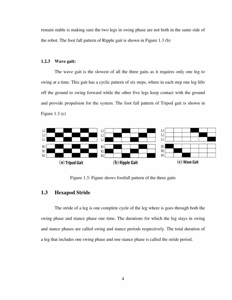
4
remain stable is making sure the two legs in swing phase are not both in the same side of
the robot. The foot fall pattern of Ripple gait is shown in Figure 1.3 (b)
1.2.3 Wave gait:
The wave gait is the slowest of all the three gaits as it requires only one leg to
swing at a time. This gait has a cyclic pattern of six steps, where in each step one leg lifts
off the ground to swing forward while the other five legs keep contact with the ground
and provide propulsion for the system. The foot fall pattern of Tripod gait is shown in
Figure 1.3 (c)
Figure 1.3: Figure shows footfall pattern of the three gaits
1.3 Hexapod Stride
The stride of a leg is one complete cycle of the leg where is goes through both the
swing phase and stance phase one time. The durations for which the leg stays in swing
and stance phases are called swing and stance periods respectively. The total duration of
a leg that includes one swing phase and one stance phase is called the stride period.

5
1.3.1 Stride period:
This is the time taken by the leg of the robot to complete one swing phase and one
stance phase. This parameter plays a key role in defining the body velocity of the system.
It is considered as one complete cycle of the leg where the phase of the leg goes from 0 to
360 degrees. At the start of the next cycle, the phase is reset to 0. Duty factor is used to
decide the ratios of swing and stance period in one stride period. All the legs of the
system follow the same values of stride, swing and stance period when implementing a
particular gait.
Since the phase of the leg is cyclic in nature, the representation of it is in two
forms in this documentation. It is either represented as a value ranging from 0 to 1, or as a
value ranging from 0 to 360(deg). It should be understood that a phase of 0.5 (for
example) is equal to the phase of 180deg.
1.3.2 Stance period:
This is the time duration in a cycle for which the leg is in contact with the ground.
During this period, all the legs in stance phase together provide support to the robot and
help propel it forward. They also help determine the stability of the system during
locomotion.
1.3.3 Swing Period:
This is the time duration for which the leg lifts off the ground and swings forward
to take the next step is called the swing period. The legs in swing phase are only
responsible to take a step forward to provide support before the other set of legs begin to

6
leave the ground. The leg in flight can potentially move faster or slower than normal, as
long as the robot remains within valid configurations.
1.3.4 Stride Length
The stride length of the system is the distance covered by the leg from taking off
the ground to touching down to the ground. The stride length of a robot is a very
important factor as helps define the speed of the robot, since if more distance is covered
with each step, the robot walks farther in less time. This parameter also helps prevent the
collision of the legs while walking as each leg can be confined to move within the stride
length itself.
1.3.5 Duty Factor:
The duty factor is the ratio of the stance period of the leg to its total stride period.
The value of the duty factor always ranges between 0 and 1, and holds true for all the legs
of the system while walking in a particular gait. The duty factors of the three gaits is as
shown in Figure 1.3
1.4 Contribution
Research has been done on legged robots to find out which gait works better for a
given terrain so that the robot can change its gait accordingly [5][6][8]. There are many
strategies that implement successful transition of gaits in a Hexapod and Quadrupeds
[3][4].
One such method is presented by Gao, Ding, Deng and Liu (2016) [7], where gait
transition is obtained by using a central pattern generator. By deriving an analytical limit

7
cycle approximation of the Van der Pol oscillator, a simple diffusive coupling scheme is
used to construct a ring-shaped CPG network. By adjusting the phase lags of the CGP
network, the control strategy is capable of generating gaits and achieving transition
among gaits.
Another method of gait transition is presented by Kottege, Parkinson, Mogham,
Elfes and Singh (2015) [2], which is based on the power consumption of the robot. A
simple algorithm is written to detect the change in the power consumption of the robot
while it moves through different terrains. The robot is made to undergo gait transition
depending on the amount of power consumed by the system during locomotion so as to
maximize the power efficiency for that terrain.
Though there are many such methods for gait transition, a reliable analysis of
when exactly should the transition take place in a walking robot is important, so that there
can be an assurance of stability in the locomotion of the robot during the transition
between different gaits.
This thesis work therefore focuses on presenting a strategy that helps figure out
leg phases at which the transition can be initiated to minimize cost of transition. A
hexapod robot is used that can walk in three different gaits: Tripod gait, Ripple gait, and
Wave gait, all on a flat terrain. The goal is to optimize the transition of the robot between
these gaits by analyzing its stability during motion as the transition is initiated at different
times during the stride, called the phase here.
A reliable phase at which each transition can be implemented is analyzed with the
help of a calculated cost of transition. The cost of transition is based on two elements: the

8
roll and pitch of the robot (or tilt motions), and the general body stability margin. The roll
and pitch of the robot is based on the sequence in which the legs lift off and touch the
ground, and are obtained from simulation of the walking robot using RoboDynaMechs as
it transitions between gaits. The stability margin of the system relies upon computation of
the support polygon which is done using MATLAB. These values are then combined to
determine the cost of transition as the function of the ‘phase at transition’. Thus the
optimum phase at which each transition can be initiated is determined.

9
Chapter 2: Concepts
2.1. Introduction
This chapter focuses on explaining about all the concepts and equations used
throughout this thesis work. It has four sections in the order of implementation. The first
section gives the method used to generate gaits. The same equations can induce transition
in the gaits when a few parameters are changed. The next section explains a method to
calculate the static stability margin of the system. This is later used in calculating the cost
of transition. The last section of this chapter explains how optimization in gait transition
is carried out. After all the concepts and related equations are presented, the next chapter
shows how these are implemented in MATLAB and RoboDynaMechs.
2.2. Gait Generation and Transition Strategy
There are many different strategies used to obtain a gait transition in hexapod,
each based on its unique requirements and functions, as described in section 1.4 of this
document. The strategy used as a part of this thesis work is built using non-linear
oscillators with phase resetting [9]. As the hexapod model used for this thesis work is
used only on a flat terrain, the parameters that initiate gait transition are solely based on
the phase of the robot. The algorithm implemented is as given below:
Trajectory generator:
∅ is used for the phase of Leg i oscillator, which generators the desired
movements for Leg i. The desired leg movements are designed based in the desired
trajectory of the leg tip relative to each body in the pitch plane, which is composed of

10
swing and stance phases. The swing phase is a simple closed loop curve that includes an
anterior extreme point (AEP) and a posterior extreme point (PEP). The stance phase is
comprised of a straight line from landing position (LP) to point PEP, as shown in Figure
2.1. When the leg tip touches the ground, LP=AEP. Thus the desired motion is provided
as a function of phase ∅ , where we used ∅ = at PEP and ∅ = ∅ 𝐸𝑃 = 𝜋 − 𝛽 at
point AEP.
Figure 2.1: Trajectories of the legs composed of swing phase and stance phase
Gait generator
The gait pattern is determined by the phase difference between the oscillators,
which is given by a matrix ∆ ≤ ∆ ≤ 𝜋 as follows:
∆ = ∅ − ∅ , , = , , … 6 (2.1)
Since ∆ = −∆ , ∆ = ∆ + ∆ , and ∆ = are satisfied, the gait pattern is
determined by five state variables, such as [∆ , ∆ , ∆ , ∆ , ∆ ].

11
The gait generator produces the desired relationship between oscillators ∆̂ based
on the desired gait pattern.
Rhythm generator:
The rhythm generator produces the basic locomotor rhythm by using leg 1,2,...,6
oscillators. The oscillator phase ∅ = , … ,6 follows the dynamics
∅̇ = 𝜔 + 𝑔 + 𝑔 , = , , … 6 (2.2)
Where 𝜔 is the basic oscillator frequency that uses the same value among the
oscillators, 𝑔 is the function regarding the gait pattern shown below and 𝑔 is the
function for phase resetting by touch sensor signals given below.
We denote the swing and stance phase durations by and respectively, for
the case when the leg tip touchesthe ground. The nominal duty factor 𝛽 and the nominal
basic frequency 𝜔 are then given by,
𝛽 = 𝑤+ (2.3)
𝜔 = 𝜋𝑤+ (2.4)
These values are satisfied regardless of the gait pattern. In this thesis work, the
swing phase duration = . sec is used.
Gait Pattern control:

12
The function 𝑔 controls the phase difference between the oscillators based on
the desired gait pattern, which is given by,
𝑔 = − ∑ sin ∅ − ∅ − ∆̂= , = , , . .6 (2.5)
Where is the gain constant.
As the value of is increased, the gait transition takes place faster, i.e., in lesser
number of steps. For this thesis work, is a matrix with all elements equal to 25.
Phase resetting:
Locomotor rhythm and phase are regulated through the modulation of motor
commands based on sensory information to create adaptive walking in biological
systems. This mechanism has been used for various legged robots. The function 𝑔 corresponds to phase resetting based on touch sensor signals. When the tip of the leg i
lands on the ground, phase ∅ of leg i oscillator is reset to∅ 𝐸𝑃 from ∅ 𝑑at the landing.
Thus 𝑔 is written by
𝑔 = (∅ 𝐸𝑃 − ∅ 𝑑)𝛿( − 𝑑), = , , … 6 (2.6)
Where 𝑑 is the time when the tip of leg i touches the ground and 𝛿 . denotes
Dirac’s delta function.
2.3. Stability Margin using Support Polygon
During locomotion of the robot, there needs to be a reliable measure of the
stability of the system. One of the most reliable methods to estimate the stability of a

13
walking robot is calculate the stability margin of the system with the help of the support
polygon [14].
The support polygon of a system at any instance is an imaginary polygon drawn
by connecting all the legs of the robot that are in the stance phase, i.e., on the ground. The
center of mass of the robot is then located and stability margin is calculated. In case the
center of mass falls out of the support polygon at any instance, the robot is said to be
unstable as the system looses it balance and falls to the ground. Such cases are to be
avoided.
Consider the robot to be walking in tripod gait as shown in Figure 2.2. In this gait
three legs are in stance phase while the other three are in swing phase. This forms a
triangle between the three points where the legs are touching the ground. The center of
the body can be marked as CB. In this position, three values, S1, S2 and S3, are
computed following the equation below:
= ∗ | | (2.7)
Where, are the coordinates of the center of the body,
And, , are the coordinates of two legs.
Thus, S1, S2 and S3 are the individual areas of the triangles formed by each pair of legs
and CB respectively.
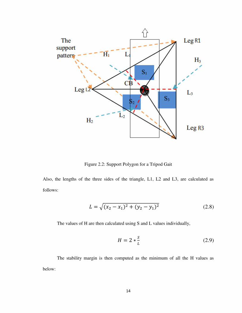
14
Figure 2.2: Support Polygon for a Tripod Gait
Also, the lengths of the three sides of the triangle, L1, L2 and L3, are calculated as
follows:
= √ − + − (2.8)
The values of H are then calculated using S and L values individually,
𝐻 = ∗ 𝐿 (2.9)
The stability margin is then computed as the minimum of all the H values as
below:

15
sm = min H , H , H , … (2.10)
This algorithm is used to calculate the stability margin values for polygons with more
than three sides obtained when the robot walks in different gaits.
It is important to mention that a positive value for stability margin is required to ensure
stability of the system.
The cost of stability is calculated for a gait over its complete stride period as the
minimum of all the observed stability margin values during the stride period. It is given
by,
𝐶 = 𝐶𝐺 = min 𝑚 , 𝑚 , 𝑚 , . . (2.11)
Similarly, the cost of stability during transition is calculated as the minimum of all the
stability margin values observed from the start of transition to the end of transition. It is
given by,
𝐶 = 𝐶 𝑁 = min 𝑚 , 𝑚 , 𝑚 , . . 𝑚 (2.12)
Where 𝑚 is a stability margin value at the start of the transition,
𝑚 is a stability margin value at the end of the transition.
2.4. Cost of Transition
During locomotion there is a variation in the roll and pitch of the robot as its legs
go through the swing and stance phases. This change in roll and pitch plays an important

16
role in the determination of the stability of the robot. A simulation software,
RoboDynamics, is used to determine this variation during locomotion of the robot.
The tilt of the robot during transition is determined by the following equation:
𝐶 = 𝑃𝑝−𝑝𝐴𝑁 ∗𝑃𝑝−𝑝𝑔 𝑖 , 𝑃𝑝−𝑝𝑔 𝑖 + 𝑝−𝑝𝐴𝑁 ∗𝑝−𝑝𝑔 𝑖 , 𝑝−𝑝𝑔 𝑖 − (2.13)
Where, 𝑃𝑝−𝑝 𝑁 represents peak-to-peak value of the pitch during transition,
𝑃𝑝−𝑝𝑔represents peak-to-peak value of the pitch during a particular gait,
𝑝−𝑝𝑁 represents peak-to-peak value of the roll during transition,
𝑝−𝑝𝑔represents peak-to-peak value of the roll during a particular gait.
The total cost of transition is determined by combining the cost of tilt with that of
the cost of stability during transition. Thus the final cost of transition is given by,
𝐶 = 𝐶 + 𝑖𝑙𝑖 𝑦 (2.14)
2.5. Optimization of Gait Transition
The optimization of gait transition is carried out by analyzing the results obtained
for the cost of transition. The three main gaits implemented as a part of this thesis are
Tripod Gait, Ripple Gait and Wave Gait. The combination of these three gaits results in
six different transitions. Each of it is tested individually by initializing the gait transition
at different values of the phase throughout the stride period and the cost is calculated for
all such tests.
17
The results are then analyzed to determine the exact value of phase at which each
transition should be initialized, so that there is an assurance of minimum stability of the
system during transition. Also, some common phenomena are observed that can be set at
guide lines to choose a phase at which the transition may take place for stable
locomotion. This is explained in detail in the Implementation section of this document.
18
Chapter 3: Implementation
3.1. Introduction
This chapter details the implementation of the concepts described in chapter 2 of
this document. It contains two sections: MATLAB and RoboDynamics. Each section
details the work done using the software, the results obtained from it, and how they have
been useful. By the end of this chapter, all work done as a part of this thesis will be
presented and the document reaches a conclusion.
3.2. MATLAB
MATLAB, Matrix Laboratory, is a very widely software for mathematical
computing. It played a significant role in the thesis work presented in this document. The
flexibility, processing speed, accuracy and simplicity of coding that this software offers
made it a highly recommended platform to base this thesis work upon. It is used to build
the architecture of the robot, the functioning behind it and obtain the results of multiple
complex iterations in as short as 3 seconds. All of the work is presented in this section
below.
3.2.1. Input Parameters to MATLAB
The hexapod robot implemented in this software abides by a few fixed parameters
to help keep the system in configuration. Also, here are some input parameters that are
varied within a specific range to help observe the nature of the system. Below are the
fixed parameters of the system:
The robot architecture is guided by the following parameters:

19
Body Length: 0.7m
Body Width: 0.15m
Leg Length: 0.12m
Distance between the legs: 0.3m
The robot locomotion is guided by the following parameters:
Stride Length: 0.2m
Stride Period: 2.0sec
Duty Factor: 0.7
With the help of these values, other important parameters are derived from the equations
in Chapter 2.
3.2.2. Work done in MATLAB
Initially in MATLAB, an experimental model of a 2D robot is built with the
dimensions as follows:
Tswing=0.12; %cm beta =0.62; %duty factor strideLength=3.2258; %cm bodyLength=10; %>3*SL bodyWidth=2.5; LegLength=2;
Three different gaits, tripod, ripple and wave, are implemented. The phases of each leg
are defined as an array as follows:
phi_tripod=[pi 0 0 pi pi 0]; phi_ripple=[4*pi/3 2*pi/3 2*pi/3 0 0 4*pi/3]; phi_wave=[0 pi pi/3 4*pi/3 2*pi/3 5*pi/3];
A complete gait generation strategy as described in section 2.2 of this document is
implemented while setting the values as given below:

20
Gain constant (K) = 20
Delta_initial = delta_desired
= matrix of the gait chosen to be implemented according to Equation (2.1)
Figure 3.1: Basic Animation of the Hexapod in MATLAB
The animation of the hexapod in MATLAB is as shown in Figure 3.1. The body
of the robot is represented in cyan. The six legs of the robot are represented in red if there
are in stance phase and white if they are in swing phase. The dotted line is the support
polygon that joins all the legs in stance phase as described in section 2.3 of this
document. The dot on the body represents the center of mass of the body. The arrow
mark indicates the direction in which the robot walks.
Figure 3.2: Tripod Gait as implemented in MATLAB

21
An example implementation of the tripod gait is as shown in Figure 3.2. The
swing and stance phases of the legs can be clearly noticed in this figure. Also, the shape
and location of the support polygon, and the location of the center of mass of the system
show how the stability margin of the system is affected during locomotion in Tripod Gait.
Figure 3.3: Stability Margin of Tripod Gait
Figure 3.3 shows the stability margin of a tripod gait for 5 seconds with the stride
period of 0.315 sec. It can be observed that there are two peak values at 3.15 each per
stride period and two angular curves. The two peaks are observed when all the six legs
are on the ground before the system takes a next step by swinging the second set of legs
forward. The angular curves are noticed when the body is propelled forwards with one set
of legs on the ground and the second set in swing phase.
22
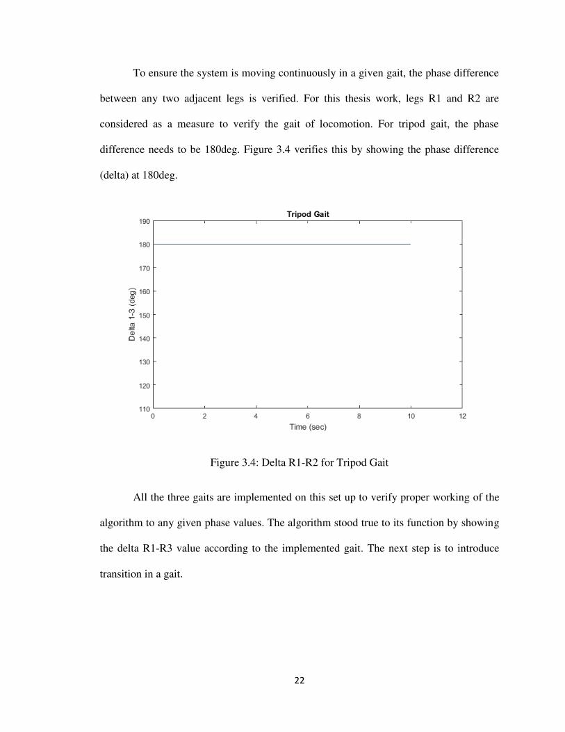
To ensure the system is moving continuously in a given gait, the phase difference
between any two adjacent legs is verified. For this thesis work, legs R1 and R2 are
considered as a measure to verify the gait of locomotion. For tripod gait, the phase
difference needs to be 180deg. Figure 3.4 verifies this by showing the phase difference
(delta) at 180deg.
Figure 3.4: Delta R1-R2 for Tripod Gait
All the three gaits are implemented on this set up to verify proper working of the
algorithm to any given phase values. The algorithm stood true to its function by showing
the delta R1-R3 value according to the implemented gait. The next step is to introduce
transition in a gait.

23
Initiating Transition at a given phase
To induce transition in a system that is walking in a stable manner is to help it
covert its walking pattern from one gait to another gradually in a few number of steps,
while trying to maintain the general stability of the system. In MATLAB, this is done by
changing the ‘desired delta’ value in Equation 2.5. That is, in case the transition should
be made from Tripod gait to Ripple gait,
Delta_initial ∆ = ∅ − ∅ =delta_tripod;
Delta_desired (∆ ̂) = delta_ripple;
Figure 3.5: Stability: Tripod Gait to Ripple Gait transition initiated at phase = 18deg
There needs to be a phase value given as input for transition to take place. This
value (∅) is exactly where the transition needs to begin. That is, when leg 1 reaches that
phase, the new value for delta_desired kicks in and aids to change the system old gait to
new gait.

24
Figure 3.6 shows a successful transition from Tripod to Ripple Gait at a phase of
108deg. More of such transitions have been tested between all three gaits. It is observed
in all cases that there was a successful transition with stable locomotion of the system.
Figure 3.6: Stability: Tripod to Ripple Gait transition initiated at phase = 108deg
The assurance of successful transition can be obtained from observing the Delta
R1-R3 values. Figures 3.7 and 3.8 show the Delta R1-R3 graphs during Tripod to Ripple
gait transition at phase = 18 deg and phase =108 deg respectively. It can be observed
from these graphs that there is a smooth and complete transition in gait from Tripod to
Ripple in approximately 4.47sec. The phase of the system successfully changes from 180
deg to 120 deg.
Next, the control of the speed of transition is to be tested.

25
Figure 3.7: Delta R1-R3: Tripod to Ripple Gait transition initiated at phase = 18deg
Figure 3.8: Delta R1-R3: Tripod to Ripple Gait transition initiated at phase = 108deg
26
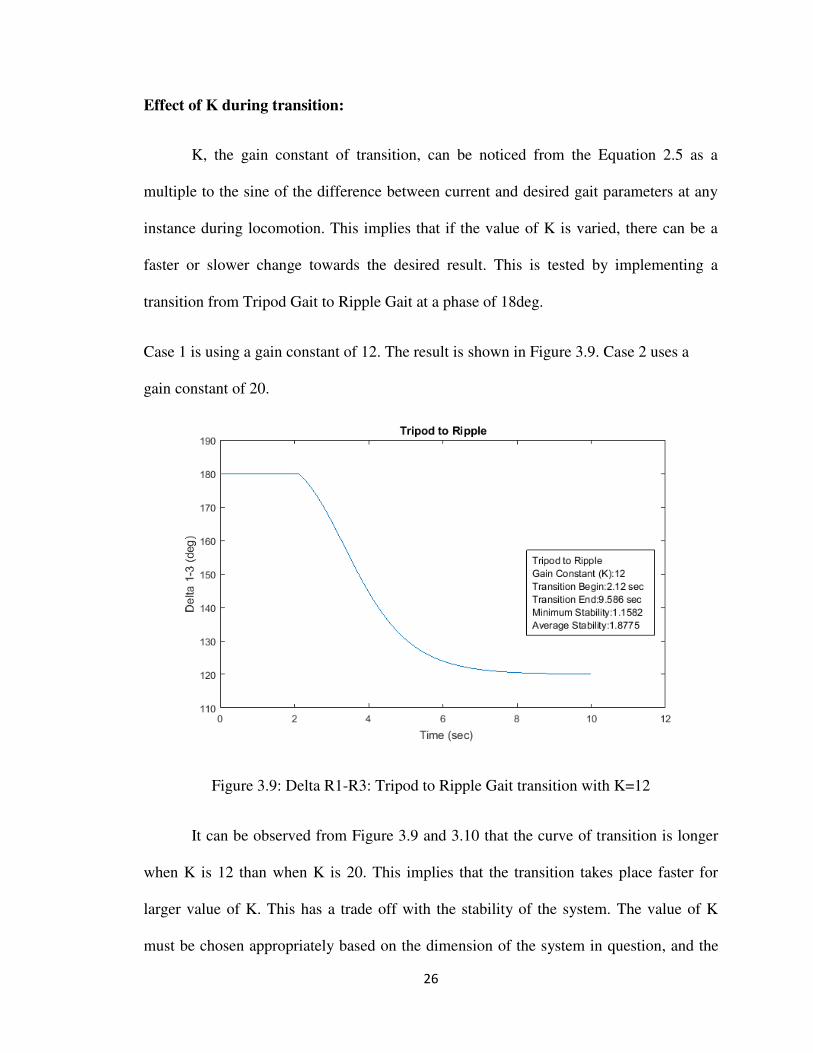
Effect of K during transition:
K, the gain constant of transition, can be noticed from the Equation 2.5 as a
multiple to the sine of the difference between current and desired gait parameters at any
instance during locomotion. This implies that if the value of K is varied, there can be a
faster or slower change towards the desired result. This is tested by implementing a
transition from Tripod Gait to Ripple Gait at a phase of 18deg.
Case 1 is using a gain constant of 12. The result is shown in Figure 3.9. Case 2 uses a
gain constant of 20.
Figure 3.9: Delta R1-R3: Tripod to Ripple Gait transition with K=12
It can be observed from Figure 3.9 and 3.10 that the curve of transition is longer
when K is 12 than when K is 20. This implies that the transition takes place faster for
larger value of K. This has a trade off with the stability of the system. The value of K
must be chosen appropriately based on the dimension of the system in question, and the

27
number of steps within which a complete transition needs to be achieved. More research
on this can be a future work of this thesis.
Figure 3.10: Delta R1-R3: Tripod to Ripple Gait transition with K=20
Introducing a larger system
The work is moved onto a larger, more practical system. Since achieving a stride
period of 0.315 seconds was not physically possible on the new system, the dimensions
and specifications of the new system are incorporated into the algorithm. Below are the
updates made to the algorithm.
Tstride=2.0; %sec beta=0.7; duty factor strideLength=20; %cm gainConstant=25; bodyLength=70; %cm bodyWidth=15; %cm LegLength=12; %cm
28
It is worth mentioning that the algorithm is built to be flexible to changes in
aspects such as stride period, duty factor, stride length, body velocity and body
dimensions.
Cost of Stability during transition
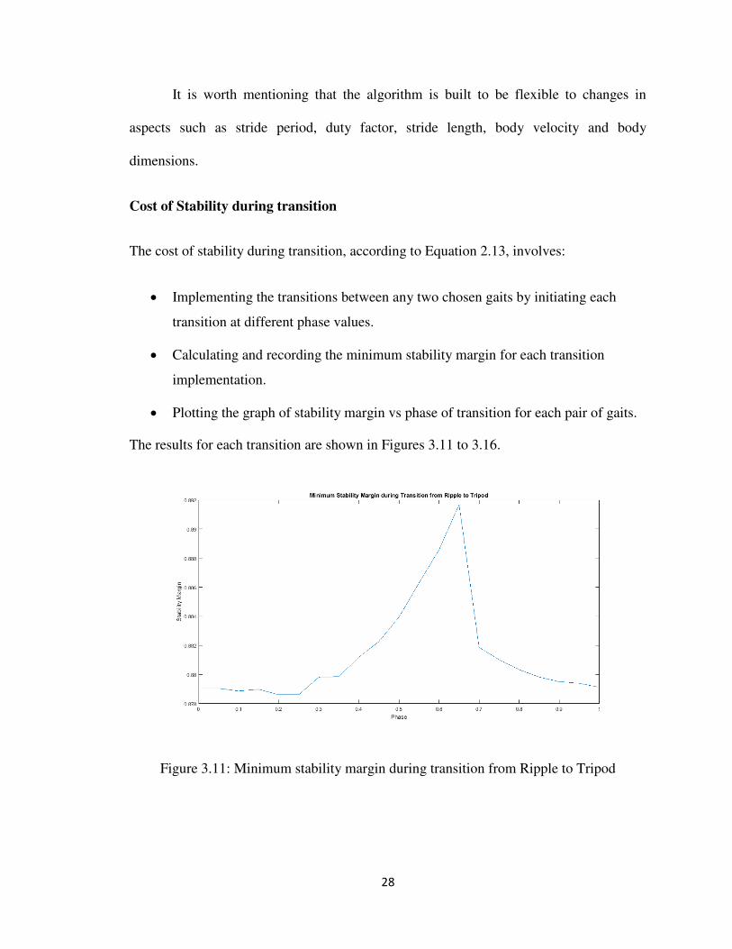
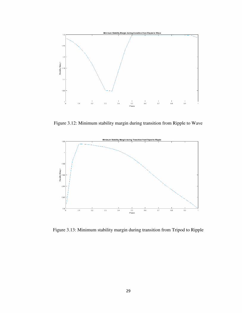
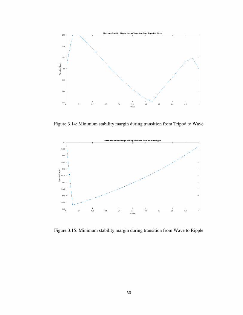
The cost of stability during transition, according to Equation 2.13, involves:
Implementing the transitions between any two chosen gaits by initiating each
transition at different phase values.
Calculating and recording the minimum stability margin for each transition
implementation.
Plotting the graph of stability margin vs phase of transition for each pair of gaits.
The results for each transition are shown in Figures 3.11 to 3.16.
Figure 3.11: Minimum stability margin during transition from Ripple to Tripod
29
Figure 3.12: Minimum stability margin during transition from Ripple to Wave
Figure 3.13: Minimum stability margin during transition from Tripod to Ripple
30
Figure 3.14: Minimum stability margin during transition from Tripod to Wave
Figure 3.15: Minimum stability margin during transition from Wave to Ripple
31
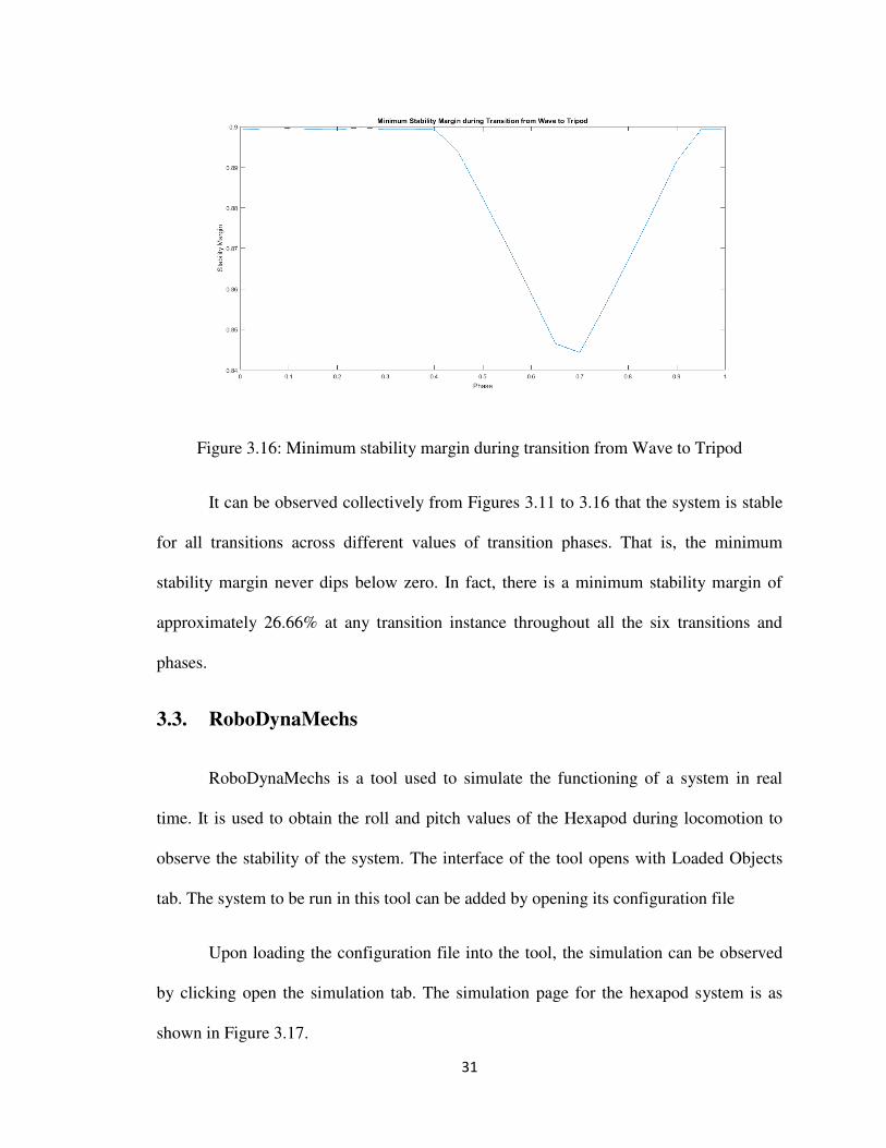
Figure 3.16: Minimum stability margin during transition from Wave to Tripod
It can be observed collectively from Figures 3.11 to 3.16 that the system is stable
for all transitions across different values of transition phases. That is, the minimum
stability margin never dips below zero. In fact, there is a minimum stability margin of
approximately 26.66% at any transition instance throughout all the six transitions and
phases.
3.3. RoboDynaMechs
RoboDynaMechs is a tool used to simulate the functioning of a system in real
time. It is used to obtain the roll and pitch values of the Hexapod during locomotion to
observe the stability of the system. The interface of the tool opens with Loaded Objects
tab. The system to be run in this tool can be added by opening its configuration file
Upon loading the configuration file into the tool, the simulation can be observed
by clicking open the simulation tab. The simulation page for the hexapod system is as
shown in Figure 3.17.

32
Figure 3.17: RoboDynaMechs GUI: Simulation tab
3.3.1. Input Parameters to RoboDynaMechs
Beside the regular inputs such as stride period, body dimensions etc,
RoboDynaMechs needs input that are specific to real time legged walking. Some of them
that are varied for the purpose of this thesis work are:
g_depressFactor = 0.92;
g_retractFactor = 0.97;
Depress Factor is a rate at which the leg of the robot moves down to the ground towards
the close of its swing phase. Retract factor is the rate at which the leg lifts off the ground
at the beginning of its swing phase. These two factors are to be balanced such that the
legs of the robot reach the ground in time before the other set of legs lifts off. For the
33
system used in this thesis work, the values of depress factor and retract factor are set to be
0.92 and 0.97 respectively.
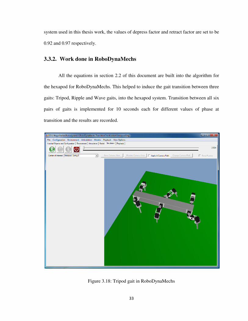
3.3.2. Work done in RoboDynaMechs
All the equations in section 2.2 of this document are built into the algorithm for
the hexapod for RoboDynaMechs. This helped to induce the gait transition between three
gaits: Tripod, Ripple and Wave gaits, into the hexapod system. Transition between all six
pairs of gaits is implemented for 10 seconds each for different values of phase at
transition and the results are recorded.
Figure 3.18: Tripod gait in RoboDynaMechs

34
The values of roll and pitch are recorded from this simulation at 1000 reading per
second. Figures 3.19 to 3.21 show the roll and pitch graphs for Tripod, Ripple and Wave
gaits respectively.
Figure 3.19: Roll and Pitch of Tripod gait
It can be observed from Figure 3.19 to 3.21 that the roll of a system increases
when there is a change in the stance leg position of the robot. That is, whenever a leg lifts
off or touches down, a disturbance in the roll of the system is noticed.
The pitch of the robot in tripod gait is observed to not vary as much as the roll
because the legs that lift off and touchdown are always balanced on either side of the
robot. This is not the case in Ripple and Wave gait and thus higher values of pitch are
observed in Ripple and Wave gait.

35
Figure 3.20: Roll and Pitch of Ripple gait
Figure 3.21: Roll and Pitch of Wave gait

36
The values for peak-to-peak roll and pitch of the three gaits are as follows:
roll_tripod= 0.044 pitch_tripod= 0.009
roll_ripple= 0.025 pitch_ripple= 0.036
roll_wave=0.039 pitch_wave=0.036
Similarly, the roll and pitch values during all six transitions are also recorded. Figure 3.22
shows the roll and pitch of the system while it transitions from Ripple gait to Wave gait
at a phase of 54deg, as an example. The transition lasted until 6sec approximately, as
indicated in the figure, and then system is observed to walk in Wave gait for the rest of
the simulation time.
Figure 3.22: Roll and Pitch of transition from Ripple gait to Wave gait

37
The cost of tilt is then calculated and recorded for different values of phases at
transition using the Equation 2.13 of this document.
3.4. Final Cost of Transition
Once the cost of transitions with respect to stability, 𝐶 , and the cost of
transition with respect to tilt, 𝐶 , are obtained, the final cost is calculated for each of
the six transitions by combining the values of 𝐶 and 𝐶 according to the
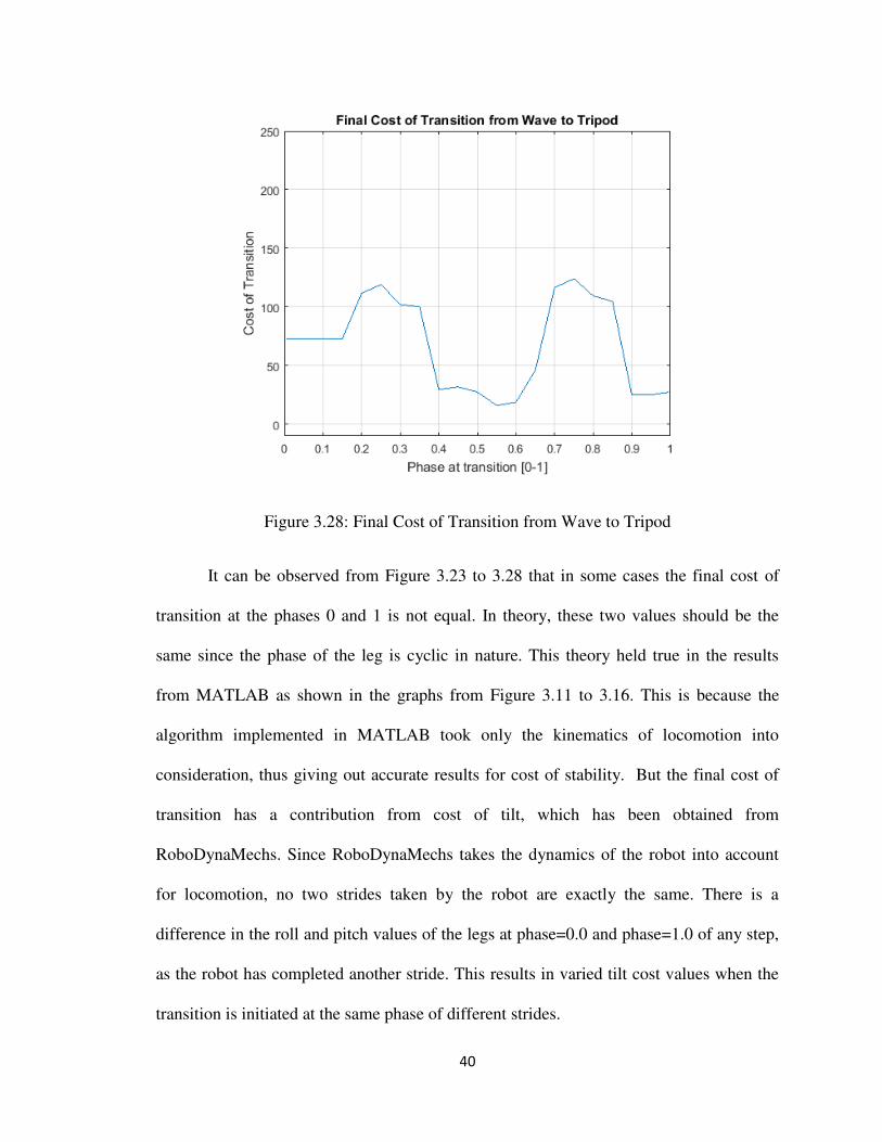
Equation 2.14 of this document. Figures 3.23 to 3.28 show the results of the final cost for
each transition.
Figure 3.23: Final Cost of Transition from Ripple to Tripod

38
Figure 3.24: Final Cost of Transition from Ripple to Wave
Figure 3.25: Final Cost of Transition from Tripod to Ripple

39
Figure 3.26: Final Cost of Transition from Tripod to Wave
Figure 3.27: Final Cost of Transition from Wave to Ripple
40
Figure 3.28: Final Cost of Transition from Wave to Tripod
It can be observed from Figure 3.23 to 3.28 that in some cases the final cost of
transition at the phases 0 and 1 is not equal. In theory, these two values should be the
same since the phase of the leg is cyclic in nature. This theory held true in the results
from MATLAB as shown in the graphs from Figure 3.11 to 3.16. This is because the
algorithm implemented in MATLAB took only the kinematics of locomotion into
consideration, thus giving out accurate results for cost of stability. But the final cost of
transition has a contribution from cost of tilt, which has been obtained from
RoboDynaMechs. Since RoboDynaMechs takes the dynamics of the robot into account
for locomotion, no two strides taken by the robot are exactly the same. There is a
difference in the roll and pitch values of the legs at phase=0.0 and phase=1.0 of any step,
as the robot has completed another stride. This results in varied tilt cost values when the
transition is initiated at the same phase of different strides.

41
To reduce these discrepancies in the future, the transition could be initiated at a
given phase value in multiple strides, and then reported as the mean of the resulting costs.
For example, the hexapod could be commanded to initiate the transition at the 0.2 phase
of stride 1, then the 0.2 phase of stride 2, and then the 0.2 phase of stride 3. The tilt cost
of transition can be computed for each stride, and then averaged such in Equation 3.1.
𝐶 [ . ] = 𝑖𝑙 𝑖 [ . ]+ 𝑖𝑙 𝑖 [ . ]+ 𝑖𝑙 𝑖 [ . ] (3.1)
The 𝐶 thus obtained is to be used to calculate the final cost of transition for each phase.
On analyzing the obtained results, the conclusions made are as follows:
The transition from Tripod to Ripple is observed to have the least cost of
transition since the Tripod gait itself has a higher peak-to-peak roll value than
peak-to-peak roll during transition at any given phase.
The cost of transition from Tripod to Wave is observed to be comparatively large.
Similar behavior is observed in transition from Wave to Tripod. This is because a
high peak-to-peak pitch value is observed during transition between these gaits.
This is due to the values of the depress factor and retract factor. Since the wave
gait needs to lift and place six legs individually within the same stride period, the
speed of movement of the legs need to be higher than for the other gaits. Thus,
this issue can be solved by varying these factors according to the gaits, which can
be a future scope of this thesis work.
According to the graphs obtained, the phases at which each transition can be
recommended to take place for lesser cost on stability of the system are:
Tripod to Ripple: 0.1 where cost is 0.09

42
Tripod to Wave: 0.4 where cost is 11.98
Wave to Tripod: 0.55 where cost is 16.02
Wave to Ripple: 0.6 where cost is 0.08
Ripple to Tripod: 0.05 where cost is 4.64
Ripple to Wave: 0.005 where cost is 10.34
43
Chapter 4: Summary
This thesis work presents a strategy to find out the phase at which the transition
between two gaits of a legged robot can be initiated to minimize the cost of transition.
The research work that has already been done towards gait transition of legged robots is
studied, and a suitable strategy has been chosen. This strategy is then implemented on a
hexapod robot across three different gaits with the help of MATLAB. Once the robot
showed successful gait generation and transition between all the three gaits, stability
analysis is conducted with the help of the support polygon. The transition between a pair
of gaits is implemented multiple times at different phase values and the minimum
stability margin is noted for each implementation. The cost of stability is then calculated.
The dynamics of the hexapod are evaluated in RoboDynaMechs and roll and pitch
of the robot are obtained for each implementation of transition between all the pair of
gaits. The cost of tilt is calculated from the obtained roll and pitch. The final cost of
transition is then calculated as the function of the ‘phase of transition’ by combining the
cost of stability and the cost of tilt. A reliable phase at which each transition can be
implemented is then analyzed with the help of the calculated cost of transition.
This strategy of determining an optimum phase to initiate the transition can be
improved by varying the fixed parameters used in the algorithm. It gives more flexibility
to the system.
44
Chapter 5: Future Work
The work completed as a part of this thesis work is the basis of much deeper work. Some
improvements that can be made to this work are:
Different values of gain constant K can be used in the algorithm to figure out how
quickly a transition can take place while maintaining the minimum cost of
transition.
Different values for Depress Factor and Retract Factor can be tested to figure out
which values work better with each transition, and if a single value can be used
with all the gait transitions while maintaining minimum cost of transition.
More gaits can be added to the algorithm to figure out which transitions work
with least possible cost.
An extension of adding more gaits could be figuring out if going through multiple
transitions instead of a single transition from current to desired gait can help to
keep the cost low. Example, while changing from Wave to Tripod in the current
work takes a minimum cost of 16.02, changing from Wave to Ripple and then
Ripple to Tripod takes only 0.08+4.64=4.72, which is even lower cost but takes
more time. This trade off can be observed further.
Long term goal of this work is the improvement of this algorithm by including all
the above work, and automating it to take a decision on when to initiate the
transition after the command to change gait is obtained and continue its
locomotion with a cost as minimum as possible.

45
Finally, all this work can be implemented on hardware and more practical results
can be obtained. This thesis work only includes software and simulation results.

46
REFERENCES
[1] G.C.Haynes, A.A. Rizzi. 2006. Gaits and Gait Transitions for Legged Robots. 2006
IEEE International Conference on Robotics and Automation (ICRA). Orlando,
Florida, May 2006.
[2] N. Kottege, C. Parkinson, P. Moghadam, A. Elfes, S.P.N. Singh. 2015. Energetics-
Informed Hexapod Gait Transitions Across Terrains. 2015 IEEE International
Conference on Robotics and Automation (ICRA). Seattle, Washington, May 26-30,
2015
[3] Liu An, Wu Heng, Li YongZheng. (2013) Gait transition of quadruped robot using
rhythm control and stability analysis. IEEE International Conference on Robotics and
Biometrics (ROBIO), Shenzhen, China, December 2013.
[4] Zhuhui Huang, Wei Wang. (2016) Controller-Switching Based Gait Transition for a
Quadruped Robot. 2016 IEEE International Conference on Mechatronics and
Automation, August 7-10, Harbin, China.
[5] Z. Yang, M. Rocha, P. Lima, M. Karamanoglu, F. Franca. (2014) A legged central
pattern generator model for autonomous gait transition. 2014 International Joint
Conference on Neural Networks (IJCNN), July 6-11, 2014, Beijing, China.
[6] W. Chen, G. Ren, J. Zhang, J. Wang. (2012) Smooth transition between different
gaits of a hexapod robot via a central pattern generators algorithm. J Intell Robot Syst
(2012) 67:255-270. DOI 10.1007/s10846-012-9661-1
47
[7] H. Yu, H. Gao, L. Ding, M Li, Z. Deng, G. Liu. 2016. Gait Generation With Smooth
Transition Using CPG-Based Locomotion Control for Hexapod Walking Robot. IEEE
Transactions on Industrial Electronics, Vol. 63, No. 9, September 2016.
[8] V. Matos, C.P. Santos, C.M.A. Pinto. (2009) A brainstem-like modulation approach
for gait transition in a quadruped robot. The 2009 IEEE/RSJ International Conference
on Intelligent Robots and Systems, October 11-15, 2009 St. Louis, USA.
[9] S. Fujiki, S. Aoi, T. Kohda, K. Senda, & K. Tsuchiya (2012). Emergence of
hysteresis in gait transition of a hexapod robot driven by nonlinear oscillators with
phase resetting, the fourth IEEE RAS & EMBS International Conference on
Biomedical Robotics and Biomechatronics, Roma, Italy. June 24-27, 2012.
[10] S. Aoi, T. Yamashita, A. Ichikawa, and K. Tsuchiya, Hysteresis in gait transition
induced by changing waist joint stiffness of a quadruped robot driven by nonlinear
oscillators with phase resetting, Proc. IEEE/RSJ Int. Conf. on Intell. Robot. Syst., pp.
1915-1920, 2010
[11] S. Aoi, T. Yamashita, and K. Tsuchiya, Hysteresis in the gait transition of a
quadruped investigated using simple body mechanical and oscillator network models,
Phys. Rev. E, 83(6):061909, 2011.
[12] T. Yamashita, S. Aoi, A. Ichikawa, and K. Tsuchiya, Emergence of hysteresis in gait
transition by changing walking speed of an oscillator-driven quadruped robot, Proc.
SICE Ann. Conf., pp. 1837-1839, 2010.
[13] S. Aoi, S. Fujiki, D.Katayama, T. Yamashita, T. Kohda, K. Senda and K. Tsuchiya.
(2011) Experimental verification of hysteresis in gait transition of a quadruped robot
driven by nonlinear oscillators with phase resetting. 2011 IEEE/RSJ International

48
Conference on Intelligent Robots and Systems, September 25-30, 2011. San
Francisco, CA, USA.
[14] F.A. Raheem, H.Z. Khaleel, (2014).Static Stability Analysis of Hexagonal Hexapod
Robot for the Periodic Gaits.ECCCM-2 Conference. IJCCCE Vol.14, No.3, 2014
[15] F.A. Raheem, H.Z. Khaleel, (2015). Hexapod Static Stability Enhancement using
Genetic algorithm. Al-Khwarizmi Engineering Journal, Vol.11, No. 4, P.P.44-59.
2015
[16] A. Skaburskyte, M, Luneckas, T. Luneckas, J, Kriauciunas, D. Udris. (2016)
Hexapod robot gait stability investigation. 2016 Advances in Information, Electronic
and Electrical Engineering (AIEEE), 2016 IEEE 4th Workshop on 10-12 Nov. 2016.
DOI: 10.1109/AIEEE.2016.7821803
[17] S. Manoiu-Olaru, M. Nitulescu. () Basic Walking simulations and gravitational
stability analysis for a hexapod robot using matlab.
[18] S. Hamdan, J. G. Fontaine, J. Rabbit, M. Picard (1990) Technics for Gait Transitions:
Architectural Considerations, IEEE International Workshop on Intelligent Robots and
Systems, IROS 1990.