an input and output excel file for a material supply
TRANSCRIPT
An input and output Excel file for a material supply assignment model
MASTER THESIS
Universiteit Gent – Industrial Management
2011/ 2012
Sergi Fabregat Corominas
Supervisor: prof. dr. ir. H. Van Landeghem
Co-supervisor: dr. V. Limère

An input and output Excel file for a material supply assignment model
Sergi Fabregat Corominas
Supervisor: prof. dr. ir. H. Van Landeghem
Co-supervisor: dr. V. Limère
MASTER THESIS
Universiteit Gent – Industrial Management
2011/ 2012
June2012

Acknowledgements
First of all, I would like to thank my promoter Hendrik Van Landeghem and my
supervisor Veronique Limère for the continuous support I have received during my stay
at Universiteit Gent. I also would like to thank to all the Industrial Management
Dempartment for offering me a workspace and for solving all my doubts during these
months.
I would also like to thank Universitat Politècnica de Catalunya and Universiteit Gent to
give me the opportunity to realize my Master thesis abroad.
Furthermore many thanks to all the friends I made during my stay in Gent. Meeting new
people from other countries is always an incredible experience and, with them, I have
lived some experiences that I will always remember.
Finally, I would like to thank my family and my friends of Barcelona. They have
supported me during all my stay abroad and have encouraged me to get the maximum
performance to this new experience. Many thanks to all of you!
Abstract
Summary
Nowadays companies need to have a competitive production system in order to face the
high competition. As it increase a lot the costs, companies realize that a way for
obtaining an advantage over their competitors is improving their logistics systems.
Although it is not a direct activity nearly linked to the company target, at the present
time most of the companies have a specific department (it could be either of their own
property or an external firm) in order to improve their logistics organizations and
supply chain methods.
Even though it depends on the type of company that considered, is well known that
logistics costs constitute around 10% of the final cost of the product. Because of this
considerable percentage, the optimization cost study related with the supply chain has a
lot of importance in the companies.
For all these reasons mentioned above, dr. Veronique Limère realized a study that will
be presented in the second chapter of the thesis in order to optimize the cost of the
distribution of the different parts to be treated in the different workstations in a typical
automotive industry.
vi
To achieve the objective of the study, a Mixed Integer Linear Programming Model
(MILP) was developed previously and defined each of the parameters and variables that
affect the final cost of the distribution. To obtain the optimal cost, this model informs, for
each one of the parts to be treated, which of both material supply methods, bulk feeding
or kitting must be used.
On the one hand, bulk feeding is the most simply and direct material supply system. In
this type of supply method, parts are supplied in containers to the assembly line. Each
container contains a large quantity of that type of part. Containers are stored at the
border of the line (BoL) of each assembly workstation in order to satisfy the demand
needed in each assembly line.
On the other hand, kitting system create heterogeneous packages by grouping together
the exact components that are needed in a particular assembly operation. Each kit can
containthe parts for one or more assembly operations. Kits are stored at the border of
the line (BoL) of the assembly lines in order to satisfy the demand needed in each
assembly workstation.
Based on the model mentioned, the main objective of this thesis is:
Objective 1: To develop a work tool for companies that are using the mathematical
model designed by dr. Veronique Limère. This tool has to targets: On the one hand, it has
to be able to obtain different results depending on the values of the parameters in order
that the employees can compare them. On the other hand it has to be easy to use and it
must give the results in a comfortable way in order to the employee can understand the
necessary information faster.
Moreover, this thesis has a second objective in orther to put in practice the work tool
mentioned in the first objective. It consists on:
Objective 2: Studying a particular company data. We will consider possible changes in
the way to supply parts, from the moment that parts are in the warehouses to the
moment that they are picket to be assembled. Results will be obtained and analysed for
each modification considered.
vii
To achieve these objectives the thesis follows the next structure: Firstly, in Chapter 1, an
introduction of the sector and a brief explication of the thesis of dr. Veronique Limère
are presented. In Chapter 2 is developed the tool for the companies and is explained
how it has been developed. In Chapter 3 an extended analysis is realized and finally, in
Chapter 4, conclusions are given.
viii
Table of Contents
Acknowledgements .......................................................................................................................... iv
Abstract ................................................................................................................................................ v
Table of Contents ........................................................................................................................... viii
List of Figures ................................................................................................................................... xii
List of Tables .................................................................................................................................... xvi
Notations ........................................................................................................................................ xviii
Chapter 1 Introduction ................................................................................................................ 1
1.1 Material supply systems .............................................................................................................. 2
1.1.1 Main differences between the different part feeding systems ............................ 6
1.1.2 Line stocking vs. Kitting system: Advantages and disadvantages ...................... 8
1.2 Contribution .................................................................................................................................. 12
1.2.1 Objectives .............................................................................................................................. 12
ix
1.2.2 Content ................................................................................................................................... 12
Chapter 2 Model review ............................................................................................................ 14
2.1 Material flows ............................................................................................................................... 15
2.1.1 Line stocking ........................................................................................................................ 15
2.1.2 Kitting ..................................................................................................................................... 15
2.2 Mathematical model .................................................................................................................. 17
2.2.1 Objective function .............................................................................................................. 17
2.2.2 Picking cost ........................................................................................................................... 17
2.2.3 Transport to the line ......................................................................................................... 18
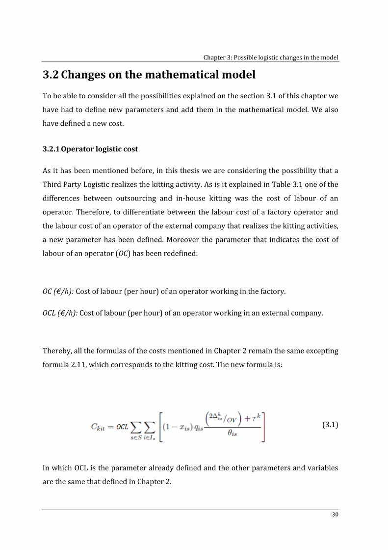
2.2.4 Kitting Cost ........................................................................................................................... 18
2.2.5 Cost of replenishment ...................................................................................................... 19
2.2.6 Restrictions ........................................................................................................................... 19
Chapter 3 Possible logistic changes in the factory ........................................................... 20
3.1 Modifications considered ......................................................................................................... 20
3.1.1 New picking technology in the supermarket........................................................... 21
3.1.1.1 Pick –by-voice ........................................................................................................................ 21
3.1.1.2 Pick –by-light ......................................................................................................................... 22
3.1.1.3 Pick –by-vision ...................................................................................................................... 23
3.1.2 Outsourcing .......................................................................................................................... 24
3.1.3 New transport equipment .............................................................................................. 25
3.1.4 Kits Batch size ...................................................................................................................... 25
x
3.1.5 Length available at the workstation ........................................................................... 29
3.1.6 Total volume of a kit .......................................................................................................... 29
3.1.7 Other possible modifications ......................................................................................... 29
3.2 Changes on the mathematical model .................................................................................. 30
3.2.1 Operator logistic cost ........................................................................................................ 30
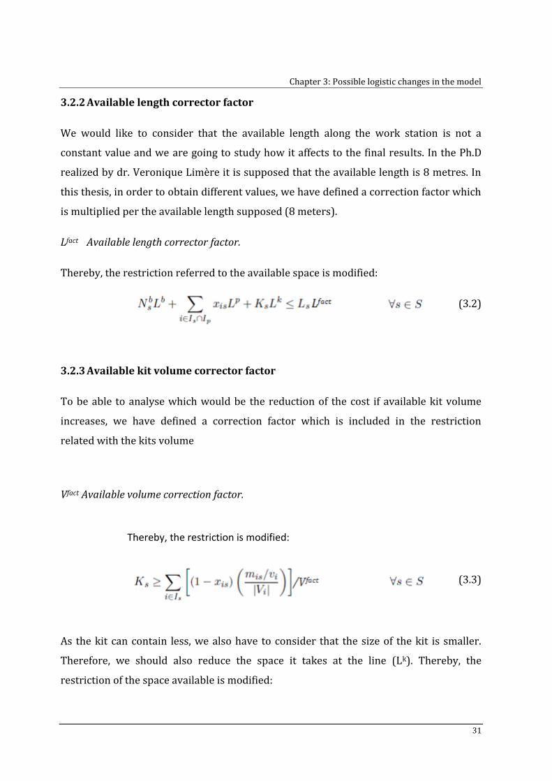
3.2.2 Available length corrector factor ................................................................................. 31
3.2.3 Available kit volume corrector factor......................................................................... 31
3.2.4 Cost of replenishment of the 3PL ................................................................................. 32
3.2.5 Forklift distance corrector factor ................................................................................. 32
3.3 Conclusions ................................................................................................................................... 33
Chapter 4 Company work tool ................................................................................................ 34
4.1 Front-end: Excel file developed ............................................................................................. 35
4.1.1 Structure of the files .......................................................................................................... 35
4.1.2 Input: Template .................................................................................................................. 37
4.1.3 Output: Table of results and graphs ............................................................................ 40
4.2 Back-end: Model files ................................................................................................................ 50
4.2.1 Model file: Defining the parameters of the template ............................................ 50
4.2.2 Data file: Reading the template ..................................................................................... 51
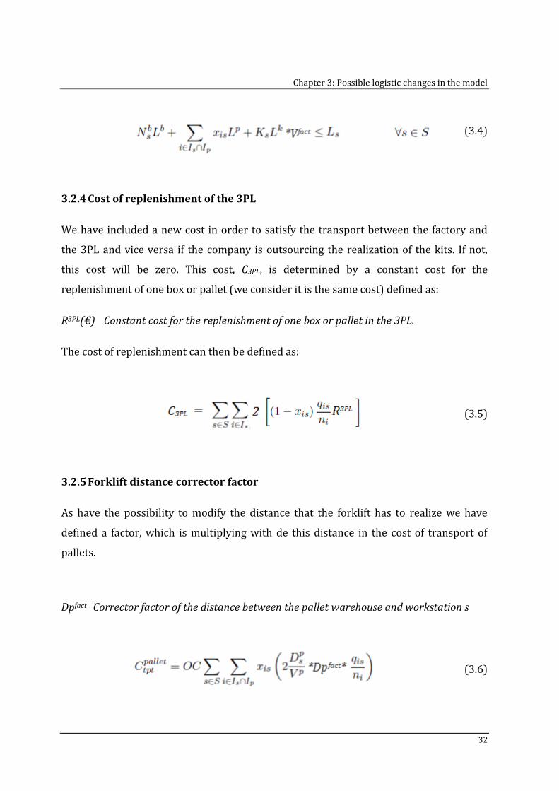
4.2.3 Run file: Algorithm designed and writing the output .......................................... 52
4.3 Instructions to use it .................................................................................................................. 54
Chapter 5 Computational results .......................................................................................... 56
xi
5.1 New picking technologies ........................................................................................................ 57
5.1.1 In the supermarket ............................................................................................................ 58
5.1.2 In the supermarket and in the assembly line .......................................................... 60
5.2 Outsourcing ................................................................................................................................... 62
5.2.1 Impact of the labour cost ................................................................................................. 63
5.2.2 Impact of the distance ...................................................................................................... 65
5.2.3 Comparison with the initial situation ......................................................................... 68
5.3 New transport equipment ....................................................................................................... 69
5.3.1 New forklift equipment .................................................................................................... 69
5.3.2 New tugger train for kits ................................................................................................. 72
5.4 Kit batch size ................................................................................................................................. 75
5.5 Available space at the border of the line ............................................................................ 77
5.6 Total volume of a kit .................................................................................................................. 80
Chapter 6 Conclusions ............................................................................................................... 82
References ......................................................................................................................................... 85
List of Figures
Figure 1.1: Picture of a BoL with containers used in the line stocking method .......................... 3
Figure 1.2: Impact of different line feeding methods on the display of parts at the border of
the line (Limère, 2011). .................................................................................................................................. 4
Figure 1.3: Flow of material for the different supply methods. ........................................................ 6
Figure 1.4: Reduction or increase of the cost if there is a change on the supply method
depending on the parameter. ....................................................................................................................... 7
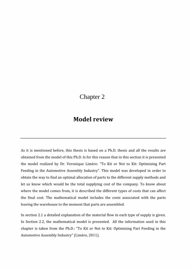
Figure 2.1: Forklift truck carrying a pallet ........................................................................................... 16
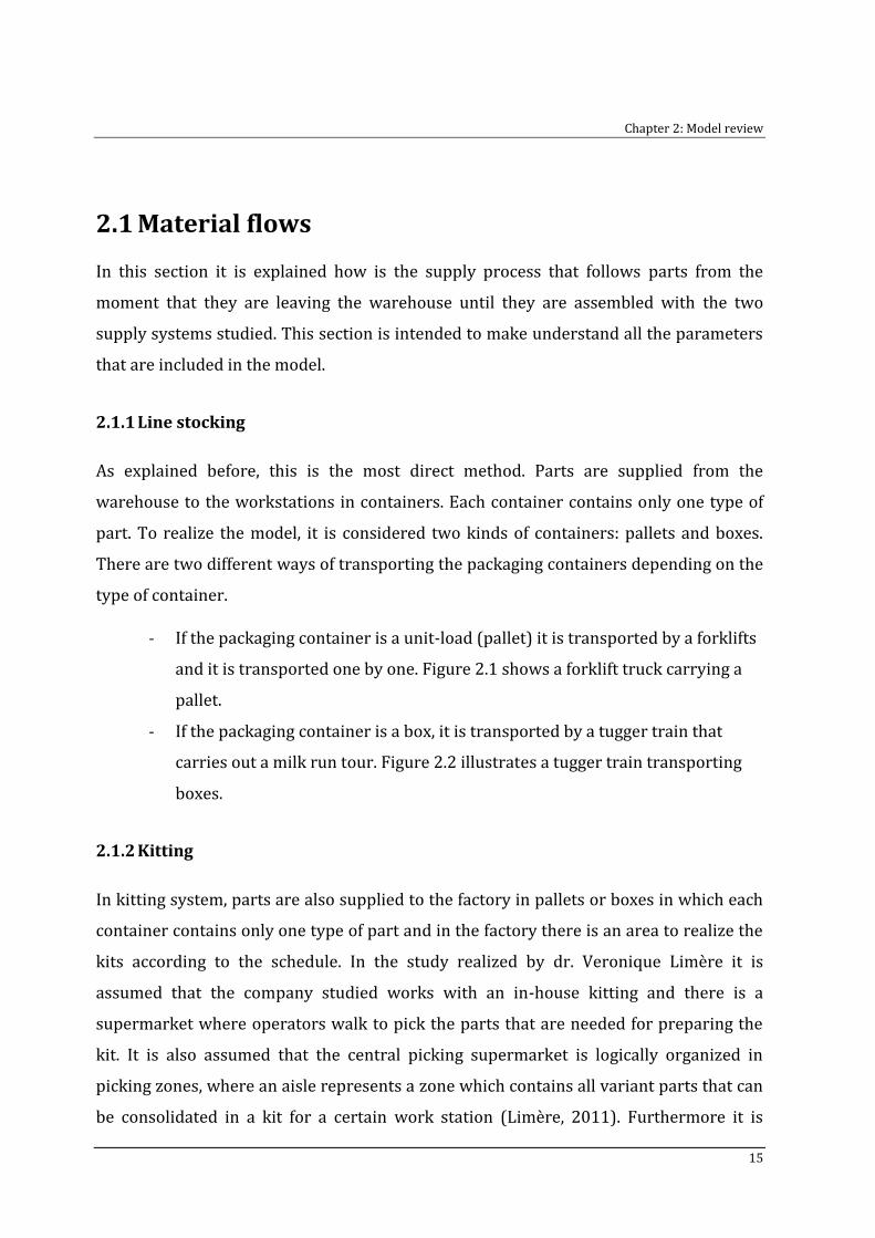
Figure 2.2: Tugger train carrying boxes ................................................................................................ 16
Figure 3.1: Operator using the pick to voice system .......................................................................... 22
Figure 3.2: Display used in a pick to light system ............................................................................... 22
Figure 3.3: Information given by the display ....................................................................................... 23
Figure 3.4: Display used in a pick-to-vision system............................................................................ 23
Figure 3.5: θ value for a particular part depending on the batch size. ....................................... 28
xiii
Figure 3.6: Kitting cost for a particular part depending on the batch size. .............................. 28
Figure 4.1: Link between the Company work tool and the model................................................. 35
Figure 4.2: Formula created for obtain the results in the graphs ................................................. 43
Figure 4.3: Formula for recognizing the feasibility of the results. ................................................ 43
Figure 4.4: Algorithm for recognizing the feasibility. ....................................................................... 44
Figure 4.5: Example of results obtained with the macro OBTAINCOMBINATIONS ................ 46
Figure 4.6: Formula for obtaining the parameter values from the values obtained with the
macro ................................................................................................................................................................. 47
Figure 4.7: Algorithm for obtaining all the parameters combination ........................................ 48
Figure 4.8: Algorithm for obtaining results in table .......................................................................... 50
Figure 4.9: Definition of the three parameters created in the template. OPERARI COST ..... 50
Figure 4.10: Example of the definition of a table and the order to read it. OPERARI COST. 51
Figure 4.11: Example of a creation of a set and the values that it takes. OPERARI COST. ... 52
Figure 4.12: Algorithm for obtaining the results ................................................................................ 54
Figure 4.13: Window to introduce the number of results. ............................................................... 55
Figure 5.1: Effect of the searching time in the supermarket in the total cost. .......................... 58
Figure 5.2: Effect of the searching time in the supermarket in the percentage of parts
kitted. ................................................................................................................................................................. 59
Figure 5.3: Effect of the searching time in the supermarket on the cost of kitting. ................ 60
Figure 5.4: Effect of the searching time at the line in the total cost. ........................................... 61
Figure 5.5: Effect of the searching time at the line in the cost to pick from a bulk. ................ 62
Figure 5.6: Effect of the searching time at the line in the percentage of parts kitted. ........... 62
xiv
Figure 5.7: Impact of the kitting labour cost of an operator in the total cost. ......................... 64
Figure 5.8: Impact of the kitting labour cost of an operator in the kitting cost. ..................... 64
Figure 5.9: Impact of the kitting labour cost of an operator in the percentage of parts
kitted. ................................................................................................................................................................. 65
Figure 5.10: Impact of the distance between the warehouse and the 3PL in the percentage
of kitting. .......................................................................................................................................................... 66
Figure 5.11: Impact of the distance between the warehouse and the 3PL in the total cost. 67
Figure 5.12: Impact of the distance between the warehouse and the 3PL in the kitting cost.
............................................................................................................................................................................. 67
Figure 5.13: Impact of the distance between the warehouse and the 3PL in the cost of
replenish the 3PL. .......................................................................................................................................... 68
Figure 5.14: Impact of the forklift velocity in the total cost ........................................................... 70
Figure 5.15: Impact of the forklift velocity in the cost of transport pallets ............................... 70
Figure 5.16: Impact of the forklift velocity in the number of kits used. ...................................... 71
Figure 5.17: Impact of the forklift velocity in the percentage of parts kitted. .......................... 71
Figure 5.18: Impact of the kits tugger train velocity in the total cost ......................................... 72
Figure 5.19: Impact of the kits tugger train velocity in the cost of transport the kits. .......... 73
Figure 5.20: Impact of the kits tugger train velocity in the percentage of parts kitted ........ 73
Figure 5.21: Impact of the kits tugger train velocity in the kitting cost ..................................... 74
Figure 5.22: Impact of the kits tugger train velocity in the number of kits used ..................... 74
Figure 5.23: Impact of the kit batch size in the total cost. .............................................................. 75
Figure 5.24: Impact of the kit batch size in the percentage of parts kitted. .............................. 76
Figure 5.25: Impact of the kit batch size in the kitting cost ............................................................ 76
xv
Figure 5.26: Impact of the space available at the station in the total cost (from 8 to 16
meters). ............................................................................................................................................................. 78
Figure 5.27: Impact of the space available at the station in the total cost (from 8 to 10
meters). ............................................................................................................................................................. 78
Figure 5.28: Impact of the space available at the station in the percentage of parts kitted
(from 8 to 10 meters) ................................................................................................................................... 79
Figure 5.29: Impact of the space available at the station in the number of kits used (from 8
to 10 meters). .................................................................................................................................................. 79
Figure 5.30: Impact of the volume available in a kit in the total cost ......................................... 80
Figure 5.31: Impact of the volume available in a kit in the number of kits used ..................... 81
Figure 5.32: Impact of the volume available in a kit in the percentage of parts kitted ........ 81
List of Tables
Table 1.1: Advantages and disadvantages of line stocking and kitting ...................................... 10
Table 1.2: Advantages and disadvantages of line stoking and kitting (continued) ................ 11
Table 3.1: Outsourcing vs. In-house kitting. Advantages and Disadvantages .......................... 24
Table 3.2: Example of kitting a particular part depending on the batch size. ......................... 27
Table 4.1: Formulas for obtaining the values of the results ............................................................ 36
Table 4.2: Example of the template used in the work tool developed. ........................................ 39
Table 4.3: Formulas for obtaining the number of results given per parameter and the total
number of results. .......................................................................................................................................... 40
Table 4.4: Computational results obtained with the parameters values of table 4.2. ........... 42
Table 4.5: Matrix of the combinations of the values that the different parameters take
according to the example of the table 4.2. ............................................................................................ 44
Table 4.6: Combinations of the parameter values according to the example given in table
4.2. ...................................................................................................................................................................... 45
xvii
Table 4.7: Explication of how the table is filled ................................................................................... 49
Table 4.8: Small table for the OPERARI COST named “OPERARI_COST”: ................................... 51
Table 5.1: Initial values of the parameters ........................................................................................... 57
Table 5.2: Costs values according to the parameters values of Table 5.1 .................................. 57
Table 5.3: Parameter values for each method ..................................................................................... 68
Table 5.4: Outsourcing vs. in-house kitting .......................................................................................... 68
Notations
Sets
Set of all parts supplied in small boxes
Set of all palletized parts
Set of all parts; I = Ip ∩ Ib
Set of all parts used at station s
Set of all work stations s
Set of variant parts of i ∈ I ; the family of part i
Parameters
Maximum number of units of a part i in one pick due
to physical characteristics (weight, volume) of part i
Capacity of the milk run tours for boxes (number of
boxes per tour)
Capacity of the milk run tours for kits (number of
kits per tour)
Batch size for assembling kits
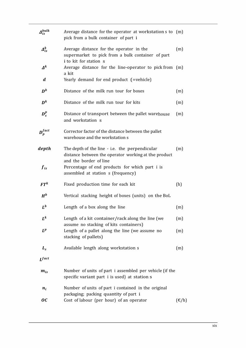
xix
Average distance for the operator at workstation s to
pick from a bulk container of part i
(m)
Average distance for the operator in the
supermarket to pick from a bulk container of part
i to kit for station s
(m)
Average distance for the line-operator to pick from
a kit
(m)
Yearly demand for end product (=vehicle)
Distance of the milk run tour for boxes (m)
Distance of the milk run tour for kits (m)
Distance of transport between the pallet warehouse
and workstation s
(m)
Corrector factor of the distance between the pallet
warehouse and the workstation s
The depth of the line - i.e. the perpendicular
distance between the operator working at the product
and the border of line
(m)
Percentage of end products for which part i is
assembled at station s (frequency)
Fixed production time for each kit (h)
Vertical stacking height of boxes (units) on the BoL
Length of a box along the line (m)
Length of a kit container/rack along the line (we
assume no stacking of kits containers)
(m)
Length of a pallet along the line (we assume no
stacking of pallets)
(m)
Available length along workstation s (m)
Number of units of part i assembled per vehicle (if the
specific variant part i is used) at station s
Number of units of part i contained in the original
packaging; packing quantity of part i
Cost of labour (per hour) of an operator (€/h)
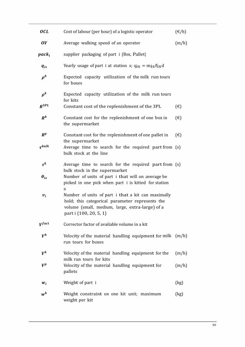
xx
Cost of labour (per hour) of a logistic operator (€/h)
Average walking speed of an operator (m/h)
supplier packaging of part i {Box, Pallet}
Yearly usage of part i at station s; qis = mis fis d
Expected capacity utilization of the milk run tours
for boxes
Expected capacity utilization of the milk run tours
for kits
Constant cost of the replenishment of the 3PL (€)
Constant cost for the replenishment of one box in
the supermarket
(€)
Constant cost for the replenishment of one pallet in
the supermarket
(€)
Average time to search for the required part from
bulk stock at the line
(s)
Average time to search for the required part from
bulk stock in the supermarket
(s)
Number of units of part i that will on average be
picked in one pick when part i is kitted for station
s
Number of units of part i that a kit can maximally
hold; this categorical parameter represents the
volume (small, medium, large, extra-large) of a
part i {100, 20, 5, 1}
Corrector factor of available volume in a kit
Velocity of the material handling equipment for milk
run tours for boxes
(m/h)
Velocity of the material handling equipment for the
milk run tours for kits
(m/h)
Velocity of the material handling equipment for
pallets
(m/h)
Weight of part i (kg)
Weight constraint on one kit unit; maximum
weight per kit
(kg)
xxi
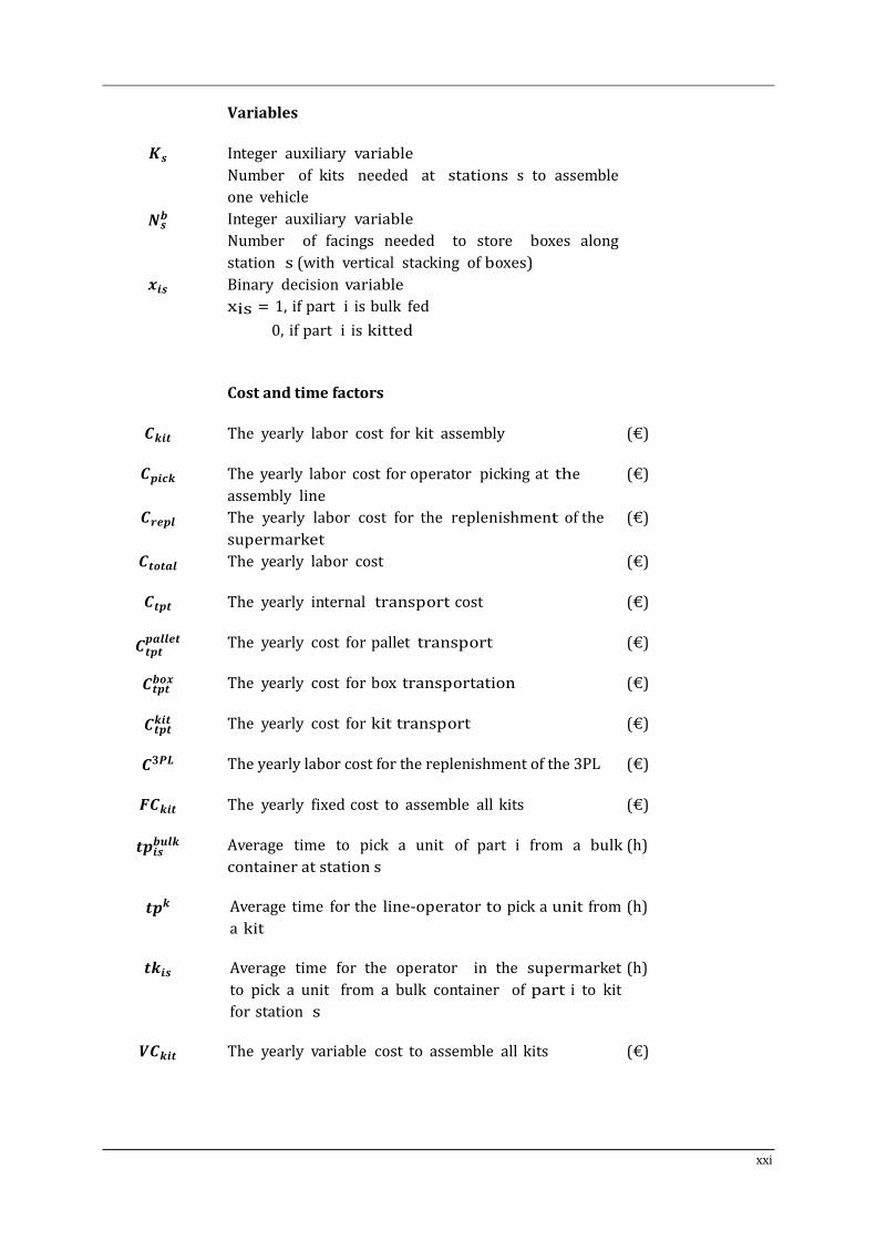
Variables
Integer auxiliary variable
Number of kits needed at stations s to assemble
one vehicle
Integer auxiliary variable
Number of facings needed to store boxes along
station s (with vertical stacking of boxes)
Binary decision variable
xis = 1, if part i is bulk fed
0, if part i is kitted
Cost and time factors
The yearly labor cost for kit assembly (€)
The yearly labor cost for operator picking at the
assembly line
(€)
The yearly labor cost for the replenishment of the
supermarket
(€)
The yearly labor cost (€)
The yearly internal transport cost (€)
The yearly cost for pallet transport (€)
The yearly cost for box transportation (€)
The yearly cost for kit transport (€)
The yearly labor cost for the replenishment of the 3PL (€)
The yearly fixed cost to assemble all kits (€)
Average time to pick a unit of part i from a bulk
container at station s
(h)
Average time for the line-operator to pick a unit from
a kit
(h)
Average time for the operator in the supermarket
to pick a unit from a bulk container of part i to kit
for station s
(h)
The yearly variable cost to assemble all kits (€)
Chapter 1
Introduction
In the field of the automotive industry, nowadays, it is required to get low prices and
timely delivery in order to obtain an advantage against the other companies competing.
For this reason, companies are trying to reduce their costs. On the one hand, companies
try to reduce the costs directly related to the vehicle manufacture, as it could be the cost
of the material of the different parts that conform the vehicle, or the cost of the energy
consumed to assemble the parts (direct costs), On the other hand, companies also try to
reduce those costs that also affects to the final cost even they are not a direct cost
(indirect costs). In this type of costs it is included the costs related to material supply
methods.
To reduce material supply costs, logistics departments have been searching the optimal
way to supply the material to the different workstations. To achieve it, companies are
investing in developing mathematical models that gives the better way to supply a
Chapter1: Introduction
2
component. These models have into account the part characteristics and plant design
and they are developed to explain us how each of the parts needed in the floor shop has
to be supplied. However, the part supply of mixed-model assembly lines is a largely
unexplored field of research (Boysen and Bock, 2011).
Because of the reasons explained above, dr. Veronique Limère realized her own model
presented on her Ph.D.: “To Kit or Not to Kit: Optimizing Part Feeding in the Automotive
Assembly Industry”. In this thesis, we will use the mentioned model developed by dr.
Veronique Limère to reach the objectives. Is for this reason that before presenting the
model, we must know how automotive industries are organized and which different
ways to supply material exists nowadays. Once we have all this information, we will be
able to understand why the model has been developed like it is.
1.1 Material supply systems
In order to be able to understand the model, it is necessary to have a previous
knowledge about the different ways that one can find in industry to supply the materials
from the warehouses to the assembly line.
Every company is allowed to choose the way to supply the material as it thought it
would be more efficient. Otherwise, it is well known that there are several supply
systems methods that usually obtain the best results and are the most typical applied
methods. These methods are explained below:
The first and most simple method is the bulk feeding or line stocking method. In this
method containers are stored at the border of the line. Each container contains one
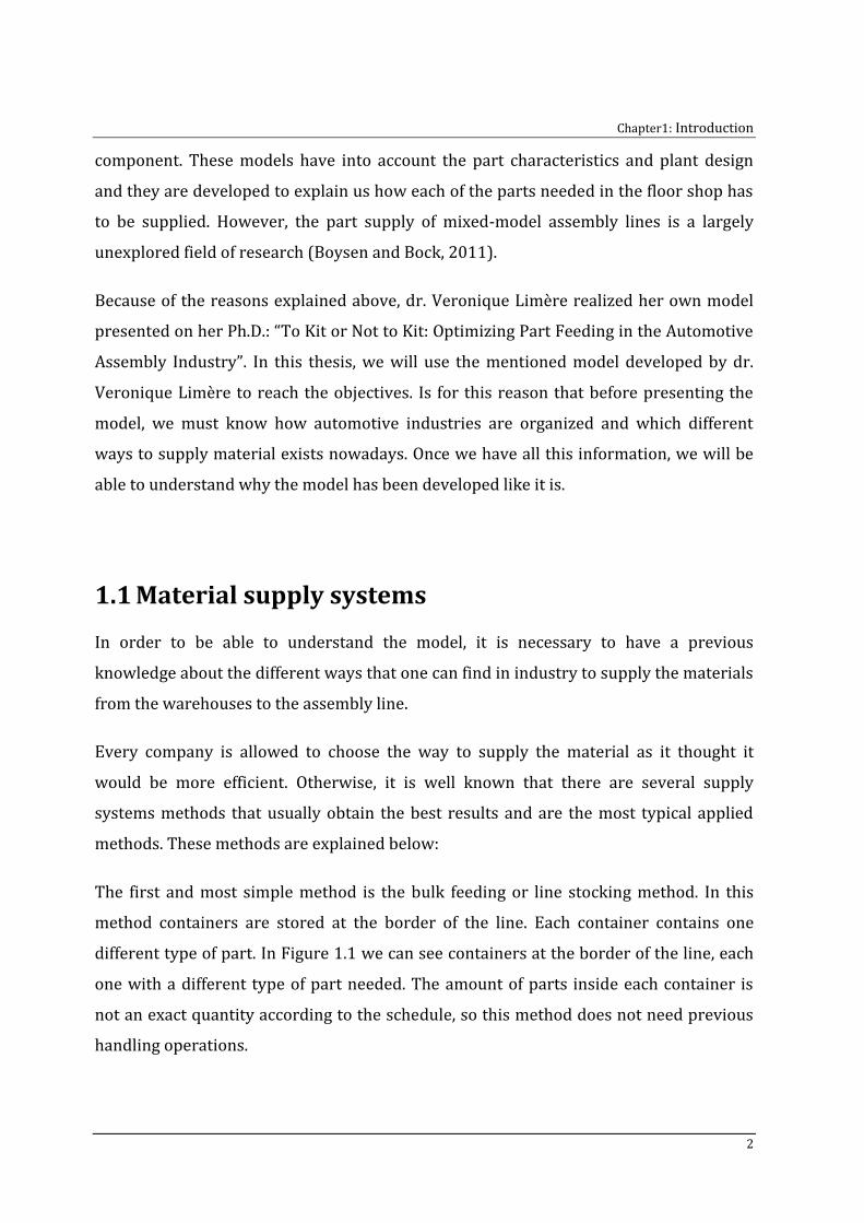
different type of part. In Figure 1.1 we can see containers at the border of the line, each
one with a different type of part needed. The amount of parts inside each container is
not an exact quantity according to the schedule, so this method does not need previous
handling operations.
Chapter1: Introduction
3
Figure 1.1: Picture of a BoL with containers used in the line stocking method
Next, we can find the downsizing method. In this case, parts are first repackaged into
smaller containers before being supplied to the workstation. Compared to a line
stocking system, downsizing needs a previous handling operation, which constitutes an
extra spent time and, consequently, an extra cost. However the fact that parts are in a
smaller bins will diminish the searching times and walking distances.
In Sequencing supply system, parts are supplied to the line at the moment that is
needed. Moreover it is supplied the exact quantity needed according to the schedule,
instead of storing the parts in containers at the border of the line. In this case, time spent
on handling operations will be even higher than with downsizing. On the other hand,
searching times and walking distances will be less than in downsizing.
Finally, the method that needs more previous work is the kitting method. Kitting is the
practice of delivering components and subassemblies to the shop floor in predetermined
quantities that are placed together in specific containers (Bozer and McGinnis, 1992).
Instead of delivering the demanded parts of each station in huge containers with large
quantities of parts, in a kitting system, the exact parts are first selected and pulled
together in kit containers before they are delivered to the workstation. Every kit
container can support more than one assembly operations. This method then also needs
Chapter1: Introduction
4
additional material handling activities, even more sophisticated than in downsizing and
sequencing. Instead of it, cost related to searching time and walking distances will be
eliminated.
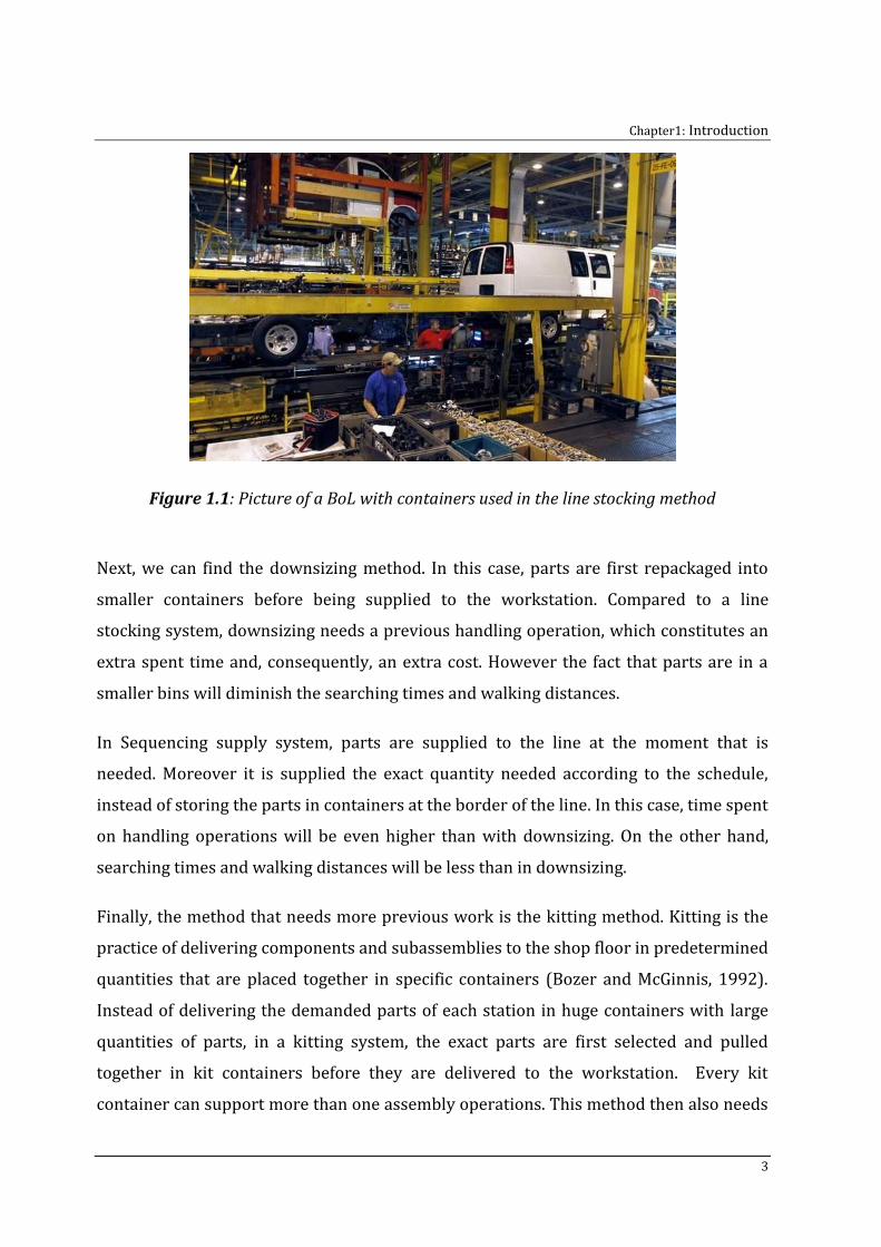
Figure 1.2 (Limère, 2011) illustrates how parts are displayed at the border of the line
depending on the material supply system. As it can be seen there is a significant
reduction of parts if we compare line stocking vs. kitting, so operator walking distances
will be reduced considerably and searching times will be eliminated if parts are
sequenced (sequencing and kitting systems). However it can be easily seen that for
displaying the material at the border of the line it is necessary more preparation time
and handling activities in kitting, sequencing or downsizing compared with line
stocking.
Figure 1.2: Impact of different line feeding methods on the display of parts at the border of the line (Limère, 2011).
Chapter1: Introduction
5
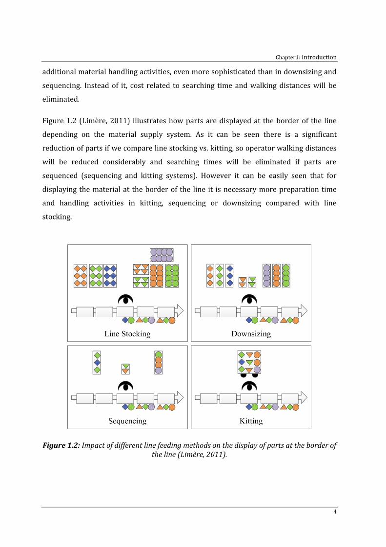
There are 3 different ways to realize the handling operations:
- The supplier is the responsible to do them so, after producing the parts to be supplied,
he has to make the kits according to the manufacturer preferences.
- The manufacturer realizes his owns kits once he has received the parts produced by the
supplier
- A Third party logistics provider (3PL) is the responsible to realize the kits.
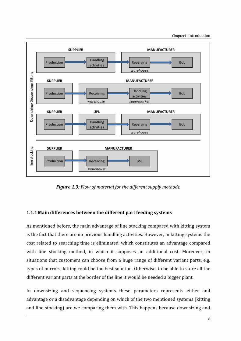
Figure 1.3 represents the basic flows of parts needed for each supply system. As we can
observe, the line stocking method only has 3 stages instead of the 4 stages that the other
methods have. It is like this due to the handling operations. This is the main advantage
that line stocking has over the other supply systems. On the other hand, with the other 3
supply systems there is lower quantity of stock at the border of the line. It means that
the operator walking distances will be reduced compared with the line stocking system.
Moreover, because of the previous handling operations done before, searching times at
the border of the line will be reduced or, in case of kitting and sequencing systems, it will
be eliminated.
Chapter1: Introduction
6
Figure 1.3: Flow of material for the different supply methods.
1.1.1 Main differences between the different part feeding systems
As mentioned before, the main advantage of line stocking compared with kitting system
is the fact that there are no previous handling activities. However, in kitting systems the
cost related to searching time is eliminated, which constitutes an advantage compared
with line stocking method, in which it supposes an additional cost. Moreover, in
situations that customers can choose from a huge range of different variant parts, e.g.
types of mirrors, kitting could be the best solution. Otherwise, to be able to store all the
different variant parts at the border of the line it would be needed a bigger plant.
In downsizing and sequencing systems these parameters represents either and
advantage or a disadvantage depending on which of the two mentioned systems (kitting
and line stocking) are we comparing them with. This happens because downsizing and
warehouse
warehouse supermarket
warehouse
warehouse
SUPPLIER MANUFACTURER
Receiving BoL
SUPPLIER 3PL
ProductionHandling
activitiesReceiving BoL
BoL
MANUFACTURER
Do
wn
sizi
ng/
Seq
uen
cin
g/ K
itti
ng
line
sto
ckin
g
Receiving
Production
SUPPLIER MANUFACTURER
ReceivingHandling
activitiesBoL
SUPPLIER
Production
MANUFACTURER
Handling
activitiesProduction
Chapter1: Introduction
7
sequencing are more moderate feeding systems and they have similarities with the
other two methods in a moderate way. We could say that talking about characteristics of
the method, they are in the middle of line stocking and kitting. Contrary, line stocking
and kitting systems are opposite methods.
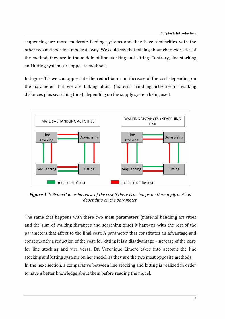
In Figure 1.4 we can appreciate the reduction or an increase of the cost depending on
the parameter that we are talking about (material handling activities or walking
distances plus searching time) depending on the supply system being used.
Figure 1.4: Reduction or increase of the cost if there is a change on the supply method depending on the parameter.
The same that happens with these two main parameters (material handling activities
and the sum of walking distances and searching time) it happens with the rest of the
parameters that affect to the final cost: A parameter that constitutes an advantage and
consequently a reduction of the cost, for kitting it is a disadvantage –increase of the cost-
for line stocking and vice versa. Dr. Veronique Limère takes into account the line
stocking and kitting systems on her model, as they are the two most opposite methods.
In the next section, a comparative between line stocking and kitting is realized in order
to have a better knowledge about them before reading the model.
WALKING DISTANCES + SEARCHING
TIMEMATERIAL HANDLING ACTIVITIES
reduction of cost increase of the cost
Line
stockingDownsizing
Sequencing Kitting
Line
stockingDownsizing
Sequencing Kitting
Chapter1: Introduction
8
1.1.2 Line stocking vs. Kitting system: Advantages and disadvantages
Once we know that the model is just taking into account line stocking and kitting
systems, in this section presents which the advantages and disadvantages are for each
type of method.
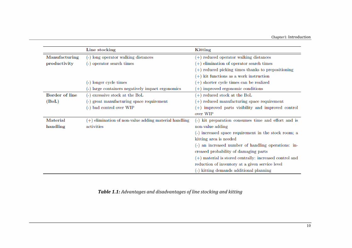
Talking about manufacturing productivity, part of the main differences that have been
commented in the previous section which were the reduction of operation walking
distances and the elimination of operator search times, there are other differences that
must be known. First of all, an advantage of kitting system that is a consequence of the
advantages commented, is the reduction of picking times because of the prepositioning.
Because of its sophisticated working method, the material in a kit may also be used as a
work instruction (Wanstrom and Melbo, 2009) and this will ease education of new staff
(Ding and Puvitharan, 1990). Moreover, when rebalancing a line, cycle time feasibility
(Swaminathan and Nitsch) has to be taken into account. The improved productivity at
the line under a kitting system will then, ceteris paribus, result in shorter feasible cycle
times (Limère, 2011). The last advantage related with manufacturing productivity is the
fact that kitting gives to the operators a better ergonomic condition.
Talking about the advantages and disadvantages of kitting and line stocking at the
border of the line, kitting system has a reduced stock, which permit to have an smaller
border of the line. Moreover, the space required to manufacture is also more reduced
than in line stocking. Finally, the number of kits provide immediate information
regarding the WIP level, since each kits consists of a predetermined quantity of parts,
and this leads to an improved control over the work-in-process (Ding and Puvitharan,
1990; Ding 1992; Choobineh and Mohebi, 2004).
Related with material handling activities, as it has been said before, line stocking system
does not need this activity, so it constitutes an advantage respect kitting. In kitting, it is
wasted a lot of time preparing the kits. Moreover, it is required an increased space in the
stock room in order to prepare the kits, and this preparation suppose an increased risk
of damaging parts because of the handling operations.
Chapter1: Introduction
9
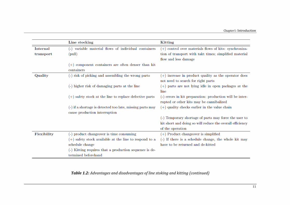
Regarding to the transport of the material, in line stocking system variable material has
to be supplied to workstations in individual component containers, which decreases the
efficiency of the plant and increases the risk of damage. In kitting, since kits are
consumed in sync with the takt time, it is easier to schedule kit replenishments than to
schedule bulk replenishments (Limère, 2011). This fact simplifies material flow.
In relation with the quality that each system gives, we must say that both methods lead
some risk of damage or schedule problems. Whereas in kitting the operator does not
need to search for the right part, in line stocking there is a risk of assemble a wrong part.
Moreover, because of the long time that parts can spend at the border of the line in line
stocking method there is a higher risk of damaging parts at the line. Otherwise, it does
not constitute a problem as relevant as in kitting because there is safety stock to replace
defective parts. In kitting, an error in kit preparation can easily produce an interruption
of the production.
Finally, if we talk about manufacturing flexibility, kitting presents some disadvantages
because it requires that a production sequence is determined beforehand (Limère,
2011). This means that it is need a long time between it is ordered and once it is
assembled. Moreover, if there is schedule change, the whole kit may have to be returned
and de-kitted (Limère, 2011).
Table 1.1 (Limère, 2011) shows a summary of the advantages and disadvantages of
kitting and line stocking explained above.
Chapter1: Introduction
10
Table 1.1: Advantages and disadvantages of line stocking and kitting
Chapter1: Introduction
11
Table 1.2: Advantages and disadvantages of line stoking and kitting (continued)
Chapter1: Introduction
12
1.2 Contribution
After having a better knowledge of the subject we need to set our objectives and the
content exposed in this thesis.
1.2.1 Objectives
In this thesis the main objective is to develop a work tool for companies using the
mathematical model designed by dr. Veronique Limère. This tool has to permit to the
employees to realize more accurate studies. We want to develop a tool in which we can
obtain different results depending on the values of the parameters and compare them.
Moreover it has to be easy to use and it must give the results in a comfortable way in
order to the employee can understand the necessary information faster.
In the background, another objective is to put this tool in practice. A study of a particular
company data will be realized. We will consider possible changes in the way to supply
parts from the warehouses to the assembly line in order to put in practice the variance
of the parameters. Results will be obtained and analysed for each modification
considered.
1.2.2 Content
The remaining part of the thesis is divided in five more chapters. In Chapter 2, it is
presented the mathematical model developed by dr. Veronique Limère. In order to
understand it, all parameters and variables that are included in the model are first
defined and explained. The whole information of this chapter is extracted from
Veronique Limère’s Ph.D. thesis: “To Kit or Not to Kit: Optimizing Part Feeding in the
Automotive Assembly Industry” where the model is presented and also explained.
Chapter 3, presents all possible changes that are considered in this thesis in the way to
supply the parts. We will also explain how it affects to the model.
In Chapter 4, the tool developed is presented. It is explained what the tool allows to do
and which information it can give to the company that is using it. Moreover it is
Chapter1: Introduction
13
explained how it has to be used. Finally, an explication of how it is linked with Limere’s
mathematical model is given.
In Chapter 5 the tool developed is put into practice by using it with a specific data of a
company. Results are given and explained in order to help the company to take
decisions.
Chapter 6 concludes the thesis.
Chapter 2
Model review
As it is mentioned before, this thesis is based on a Ph.D. thesis and all the results are
obtained from the model of this Ph.D. Is for this reason that in this section it is presented
the model realized by Dr. Veronique Limère: “To Kit or Not to Kit: Optimizing Part
Feeding in the Automotive Assembly Industry”. This model was developed in order to
obtain the way to find an optimal allocation of parts to the different supply methods and
let us know which would be the total supplying cost of the company. To know about
where the model comes from, it is described the different types of costs that can affect
the final cost. The mathematical model includes the costs associated with the parts
leaving the warehouse to the moment that parts are assembled.
In section 2.1 a detailed explanation of the material flow in each type of supply is given.
In Section 2.2, the mathematical model is presented. All the information used in this
chapter is taken from the Ph.D.: “To Kit or Not to Kit: Optimizing Part Feeding in the
Automotive Assembly Industry” (Limère, 2011).
Chapter 2: Model review
15
2.1 Material flows
In this section it is explained how is the supply process that follows parts from the
moment that they are leaving the warehouse until they are assembled with the two
supply systems studied. This section is intended to make understand all the parameters
that are included in the model.
2.1.1 Line stocking
As explained before, this is the most direct method. Parts are supplied from the
warehouse to the workstations in containers. Each container contains only one type of
part. To realize the model, it is considered two kinds of containers: pallets and boxes.
There are two different ways of transporting the packaging containers depending on the
type of container.
- If the packaging container is a unit-load (pallet) it is transported by a forklifts
and it is transported one by one. Figure 2.1 shows a forklift truck carrying a
pallet.
- If the packaging container is a box, it is transported by a tugger train that
carries out a milk run tour. Figure 2.2 illustrates a tugger train transporting
boxes.
2.1.2 Kitting
In kitting system, parts are also supplied to the factory in pallets or boxes in which each
container contains only one type of part and in the factory there is an area to realize the
kits according to the schedule. In the study realized by dr. Veronique Limère it is
assumed that the company studied works with an in-house kitting and there is a
supermarket where operators walk to pick the parts that are needed for preparing the
kit. It is also assumed that the central picking supermarket is logically organized in
picking zones, where an aisle represents a zone which contains all variant parts that can
be consolidated in a kit for a certain work station (Limère, 2011). Furthermore it is
Chapter 2: Model review
16
assumed that multiple kits of the same type are assembled in batches of five because five
kits fit on one rack (Limère, 2011). The transport from the warehouse to the
supermarket is realized, as in line stocking, in two different ways depending on the type
of container:
- By forklift if the container is a unit-load (pallet). Figure 2.1.
- By a tugger train if the container is a box. Figure 2.2.
After preparing the kits in the supermarket they are transported in kits containers (each
kit container can carry multiple kits of the same type) by a tugger train that realizes a
milk run tour. As one kit is consumed per takt time, kit container replenishments are
needed according to constant time intervals (Limère, 2011).
Figure 2.1: Forklift truck carrying a pallet
Figure 2.2: Tugger train carrying boxes
Chapter 2: Model review
17
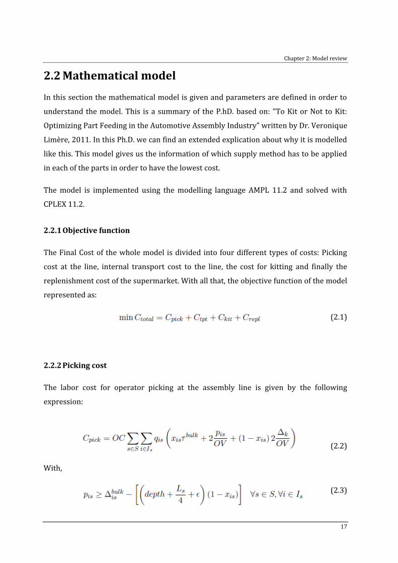
2.2 Mathematical model
In this section the mathematical model is given and parameters are defined in order to
understand the model. This is a summary of the P.hD. based on: “To Kit or Not to Kit:
Optimizing Part Feeding in the Automotive Assembly Industry” written by Dr. Veronique
Limère, 2011. In this Ph.D. we can find an extended explication about why it is modelled
like this. This model gives us the information of which supply method has to be applied
in each of the parts in order to have the lowest cost.
The model is implemented using the modelling language AMPL 11.2 and solved with
CPLEX 11.2.
2.2.1 Objective function
The Final Cost of the whole model is divided into four different types of costs: Picking
cost at the line, internal transport cost to the line, the cost for kitting and finally the
replenishment cost of the supermarket. With all that, the objective function of the model
represented as:
(2.1)
2.2.2 Picking cost
The labor cost for operator picking at the assembly line is given by the following
expression:
(2.2)
With,
(2.3)
Chapter 2: Model review
18
(2.4)
e Any small number
(2.5)
(2.6)
2.2.3 Transport to the line
The total transport cost is the sum of the costs for the different types of transportation:
trough pallets, box or kits.
(2.7)
With,
(2.8)
(2.9)
(2.10)
2.2.4 Kitting Cost
The labor cost for Kit assembly is given by:
(2.11)
Chapter 2: Model review
19
With,
(2.12)
2.2.5 Cost of replenishment
The total cost of the replenishment of the supermarket can be defined as:
(2.13)
2.2.6 Restrictions
The objective function is subjected to the constraints exposed below:
(2.14)
(2.15)
(2.16)
(2.17)
(2.18)
(2.19)
(2.20)
Chapter 3
Possible logistic changes in the factory
As we have seen in the previous chapter, the mathematical model offers the opportunity
to select, for each of the parts that have to be supplied, the material supply method
which is most cost effective for the overall material delivery system. However, some
considerations have been assumed with this model. In this thesis, we want to take into
consideration some changes that the company could realize in the way of performing the
parts supply.
In section 3.1 are presented the possible modifications that we want to consider. In
section 3.2, we expose the changes realized in the mathematical model in order to study
these considerations.
3.1 Modifications considered
As it has been explained, to create the mathematical model some parameters have been
fixed and some characteristics of the way to supply the parts have been assumed to be
Chapter 3: Possible logistic changes in the model
21
as mentioned in the first and second chapter. The aim of this section is to analyse which
variances an industry can suffer compared with the described situation.
Below are described the possible logistic modifications in the company.
3.1.1 New picking technology in the supermarket
Until this moment, it is assumed by the model that there is a central supermarket were
picking operators walk to pick the needed parts (Limère, 2011). However, there are
some technological management systems to increase the picking efficiency by minimize
picking time and reduce the errors made by the operators, which would make reduce
the costs. Three of the most known picking methods are the pick-by-voice, pick-by-light
and pick-by-vision.
3.1.1.1 Pick –by-voice
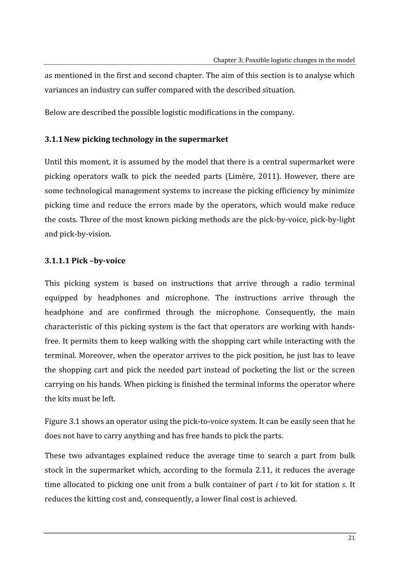
This picking system is based on instructions that arrive through a radio terminal
equipped by headphones and microphone. The instructions arrive through the
headphone and are confirmed through the microphone. Consequently, the main
characteristic of this picking system is the fact that operators are working with hands-
free. It permits them to keep walking with the shopping cart while interacting with the
terminal. Moreover, when the operator arrives to the pick position, he just has to leave
the shopping cart and pick the needed part instead of pocketing the list or the screen
carrying on his hands. When picking is finished the terminal informs the operator where
the kits must be left.
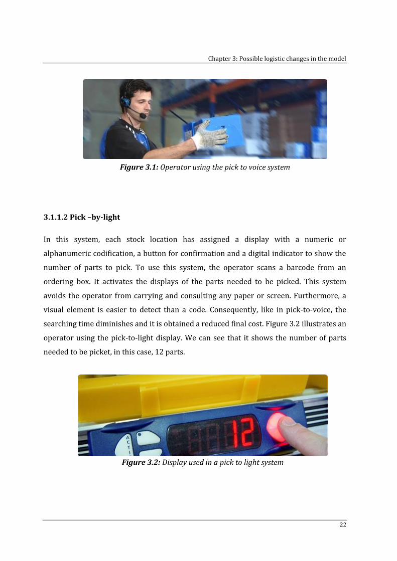
Figure 3.1 shows an operator using the pick-to-voice system. It can be easily seen that he
does not have to carry anything and has free hands to pick the parts.
These two advantages explained reduce the average time to search a part from bulk
stock in the supermarket which, according to the formula 2.11, it reduces the average
time allocated to picking one unit from a bulk container of part i to kit for station s. It
reduces the kitting cost and, consequently, a lower final cost is achieved.
Chapter 3: Possible logistic changes in the model
22
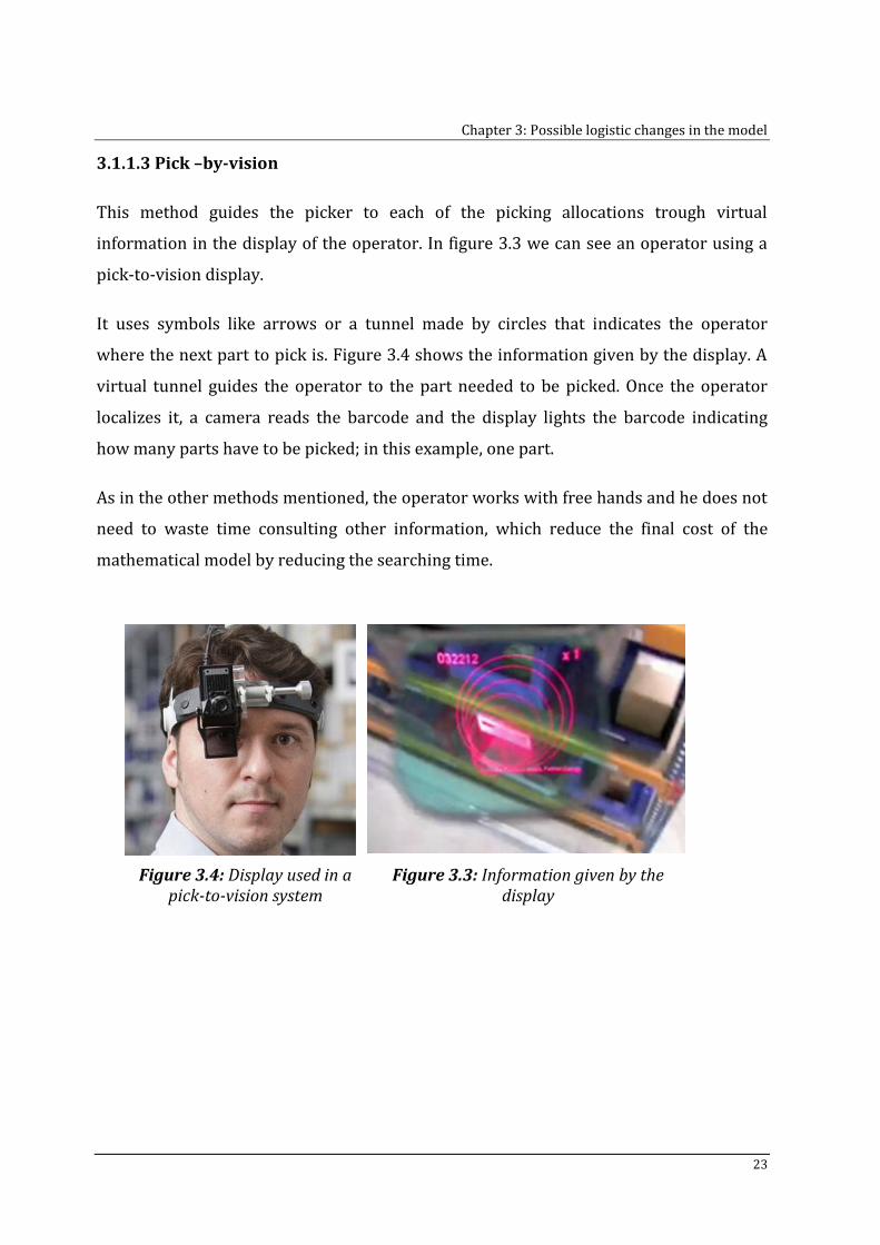
3.1.1.2 Pick –by-light
In this system, each stock location has assigned a display with a numeric or
alphanumeric codification, a button for confirmation and a digital indicator to show the
number of parts to pick. To use this system, the operator scans a barcode from an
ordering box. It activates the displays of the parts needed to be picked. This system
avoids the operator from carrying and consulting any paper or screen. Furthermore, a
visual element is easier to detect than a code. Consequently, like in pick-to-voice, the
searching time diminishes and it is obtained a reduced final cost. Figure 3.2 illustrates an
operator using the pick-to-light display. We can see that it shows the number of parts
needed to be picket, in this case, 12 parts.
Figure 3.1: Operator using the pick to voice system
Figure 3.2: Display used in a pick to light system
Chapter 3: Possible logistic changes in the model
23
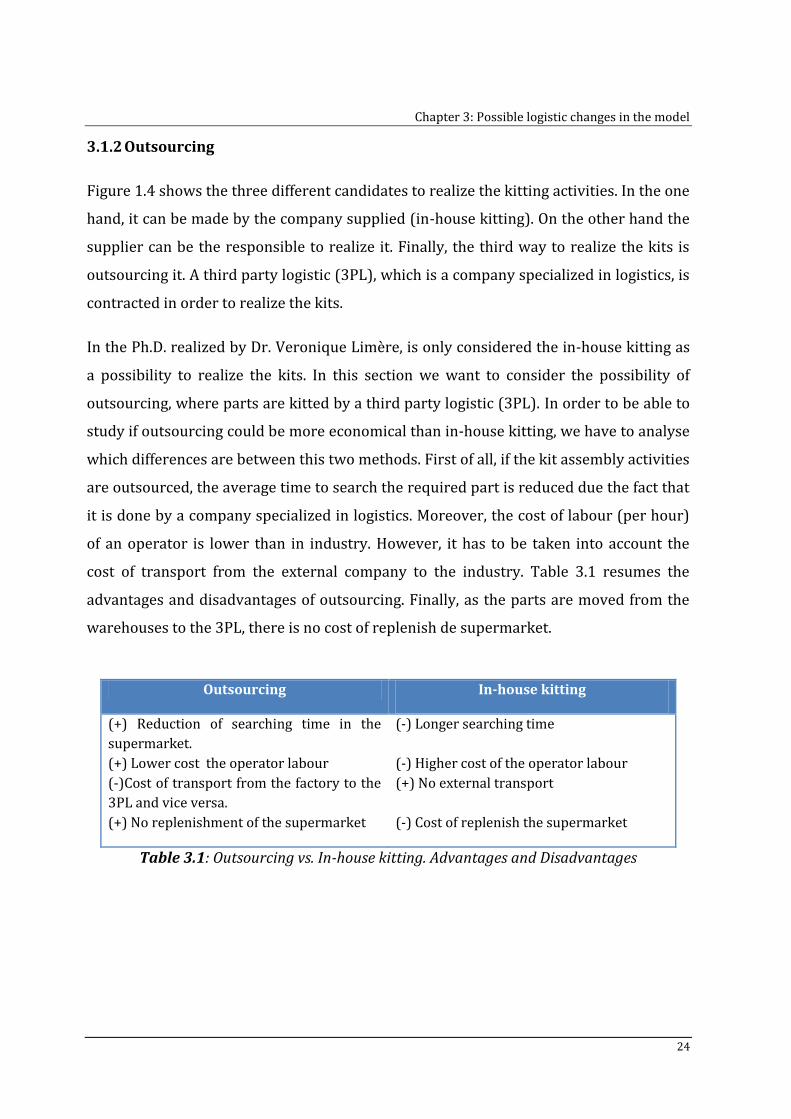
3.1.1.3 Pick –by-vision
This method guides the picker to each of the picking allocations trough virtual
information in the display of the operator. In figure 3.3 we can see an operator using a
pick-to-vision display.
It uses symbols like arrows or a tunnel made by circles that indicates the operator
where the next part to pick is. Figure 3.4 shows the information given by the display. A
virtual tunnel guides the operator to the part needed to be picked. Once the operator
localizes it, a camera reads the barcode and the display lights the barcode indicating
how many parts have to be picked; in this example, one part.
As in the other methods mentioned, the operator works with free hands and he does not
need to waste time consulting other information, which reduce the final cost of the
mathematical model by reducing the searching time.
Figure 3.4: Display used in a pick-to-vision system
Figure 3.3: Information given by the display
Chapter 3: Possible logistic changes in the model
24
3.1.2 Outsourcing
Figure 1.4 shows the three different candidates to realize the kitting activities. In the one
hand, it can be made by the company supplied (in-house kitting). On the other hand the
supplier can be the responsible to realize it. Finally, the third way to realize the kits is
outsourcing it. A third party logistic (3PL), which is a company specialized in logistics, is
contracted in order to realize the kits.
In the Ph.D. realized by Dr. Veronique Limère, is only considered the in-house kitting as
a possibility to realize the kits. In this section we want to consider the possibility of
outsourcing, where parts are kitted by a third party logistic (3PL). In order to be able to
study if outsourcing could be more economical than in-house kitting, we have to analyse
which differences are between this two methods. First of all, if the kit assembly activities
are outsourced, the average time to search the required part is reduced due the fact that
it is done by a company specialized in logistics. Moreover, the cost of labour (per hour)
of an operator is lower than in industry. However, it has to be taken into account the
cost of transport from the external company to the industry. Table 3.1 resumes the
advantages and disadvantages of outsourcing. Finally, as the parts are moved from the
warehouses to the 3PL, there is no cost of replenish de supermarket.
Outsourcing In-house kitting
(+) Reduction of searching time in the
supermarket.
(+) Lower cost the operator labour
(-)Cost of transport from the factory to the
3PL and vice versa.
(+) No replenishment of the supermarket
(-) Longer searching time
(-) Higher cost of the operator labour
(+) No external transport
(-) Cost of replenish the supermarket
Table 3.1: Outsourcing vs. In-house kitting. Advantages and Disadvantages
Chapter 3: Possible logistic changes in the model
25
3.1.3 New transport equipment
Tugger trains and forklift truck are the responsible of the internal transport. Until this
moment we assume that a specific tugger train and forklift truck is used. The tugger
train doing the milk run tour has a velocity of 2412 m/h (Vb and Vk) and it is able to
transport 60 boxes per tour (Ab) in case it is transporting boxes and 70 kits per tour (Ak)
if it is transporting kits. The forklift truck has a velocity of 2880 m/h (Vp) and it
transport the pallets one by one.
In this thesis, we want to consider the possibility of using different types of tugger trains
and forklifts to analyse which characteristics are the most rentable. We will consider
that the company uses shorter tugger trains, so the velocity will be higher and time of
transport will be diminished and consequently, the cost of transport will diminishes too.
However, it will have less capacity to carry the boxes or kits, which constitutes an
increase of the cost on peak moments.
The milk run tours take places on constant interval times and the demand varies
depending on the moment, so tugger trains are not always fully utilized. On average, the
capacity utilization for box (ρb) is supposed to be 50% and 80% for kits (ρk). We assume
that these two parameters remain constant. It is considered like this because in one
hand, the fact that the tugger train is shorter would make increase the percentage of
capacity occupied. However, on the other hand, the fact that the tugger train is faster
suppose that it is able to complete more milk run tours in the same time and it would
diminish the percentage of capacity occupied.
We will also consider the possibility that the company invests in faster forklifts.
3.1.4 Kits Batch size
On the transport from the supermarket to the assembly line, kits of the same type are
assumed to be assembled in batches of five because five kits fit on one rack (Limère,
2011). However it could happen that sometimes racks cannot be full. In this thesis we
will consider the kit batch size is not always 5 kits. It will have an impact in the kitting
cost because it has an effect on the number of units of part i that will on average be
Chapter 3: Possible logistic changes in the model
26
picked in one pick (θis). However it just has an effect on it if two conditions are satisfied.
As it is presented in Chapter 2, the opportunity for batch picking part i to assemble in a
kit for station s is defined by:
(3.1)
With,
qis Yearly usage of part i at station s
d Yearly demand for end product (= vehicle)
Bk Batch size for assembling kits
ai Maximum number of units of a part i in one pick due to physical
characteristics (weight, volume) of part i
mis Number of units of part i assembled per vehicle (if the specific variant part i is
used) at station s
When the following conditions are satisfied, the variance of the batch size has an effect
on the kitting cost:
(3.2)
(3.3)
We will give an example to understand it. We suppose that one part is kitted but the
batch size varies from 3 kits per rack to 10 kits per rack (we will not consider this
dimensions on the study but they are useful to explain the impact of the kit batch size in
the kitting cost). The other parameters (qis, d, ai, mis) will be constant because we are
working with the same part.
Chapter 3: Possible logistic changes in the model
27
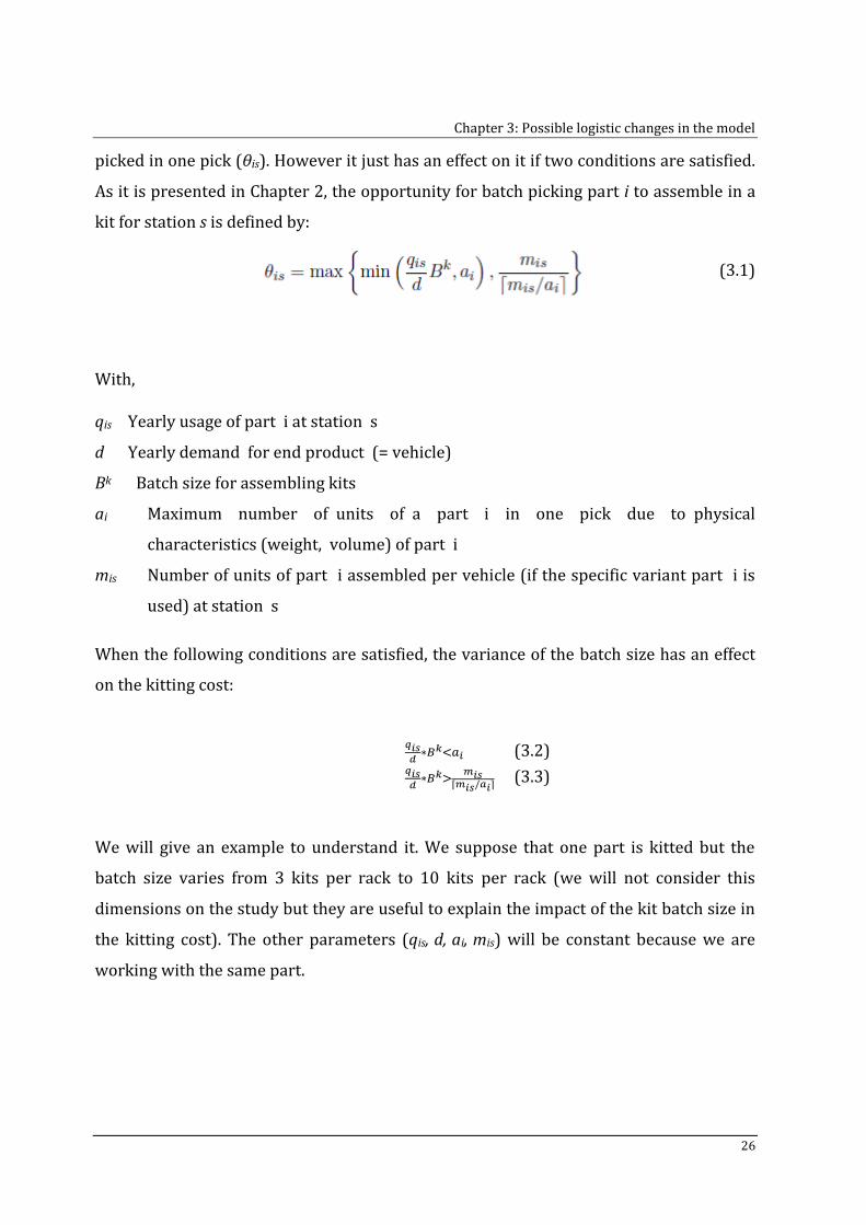
The following values are used in this example:
Batch size (kits) 3 4 5 6 7 8 9 10
1,5 2 2,5 3 3,5 4 4,5 5
4 4 4 4 4 4 4 4
2,5 2,5 2,5 2,5 2,5 2,5 2,5 2,5
2,5 2,5 2,5 3 3,5 4 4 4
Satisfies conditions? NO NO NO YES YES NO NO NO
Kitting cost 50,80 50,80 50,80 42,33 36,29 31,75 31,75 31,75
Table 3.2: Example of kitting a particular part depending on the batch size.
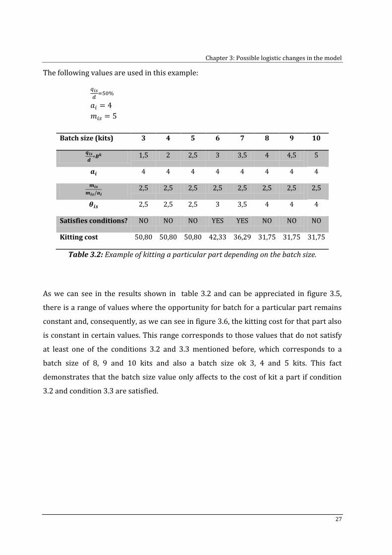
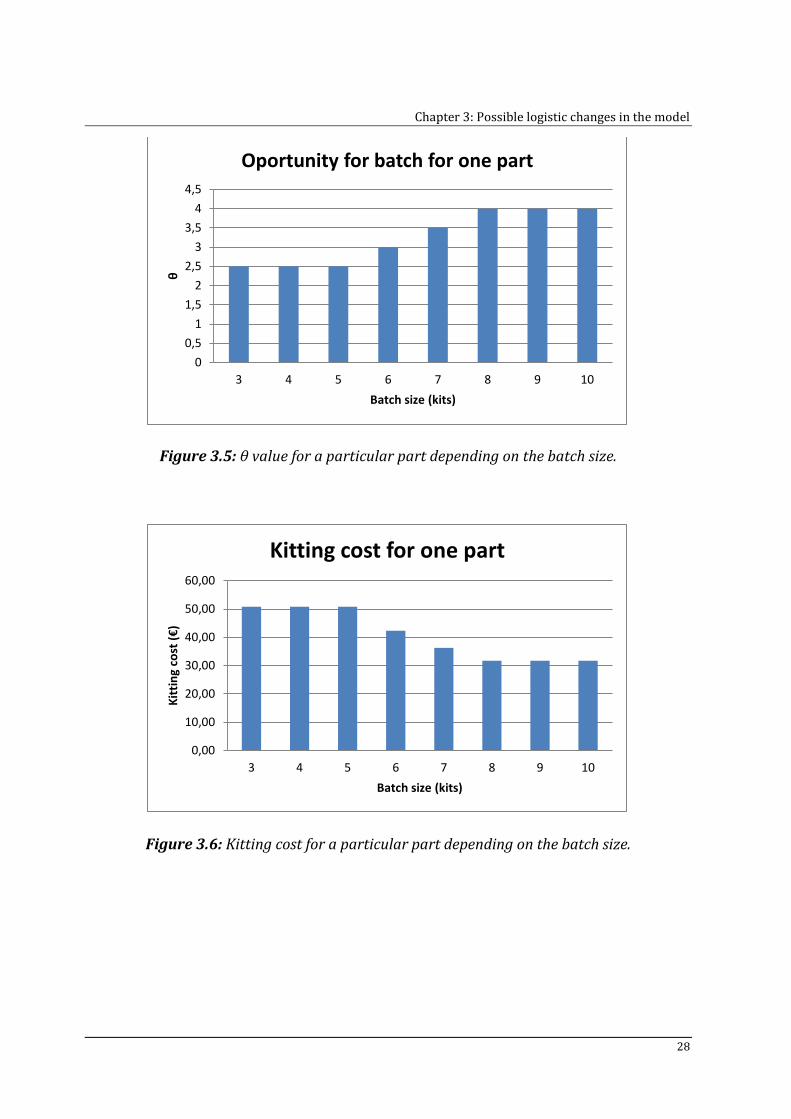
As we can see in the results shown in table 3.2 and can be appreciated in figure 3.5,
there is a range of values where the opportunity for batch for a particular part remains
constant and, consequently, as we can see in figure 3.6, the kitting cost for that part also
is constant in certain values. This range corresponds to those values that do not satisfy
at least one of the conditions 3.2 and 3.3 mentioned before, which corresponds to a
batch size of 8, 9 and 10 kits and also a batch size ok 3, 4 and 5 kits. This fact
demonstrates that the batch size value only affects to the cost of kit a part if condition
3.2 and condition 3.3 are satisfied.
Chapter 3: Possible logistic changes in the model
28
Figure 3.5: θ value for a particular part depending on the batch size.
Figure 3.6: Kitting cost for a particular part depending on the batch size.
0
0,5
1
1,5
2
2,5
3
3,5
4
4,5
3 4 5 6 7 8 9 10
θ
Batch size (kits)
Oportunity for batch for one part
0,00
10,00
20,00
30,00
40,00
50,00
60,00
3 4 5 6 7 8 9 10
Kit
tin
g co
st (€
)
Batch size (kits)
Kitting cost for one part
Chapter 3: Possible logistic changes in the model
29
3.1.5 Length available at the workstation
The available length along a workstation is a restrictive parameter. In this thesis we
want to study how it affects at the final cost. It is easy to understand that as a restrictive
parameter, when the available length along the workstation is higher, the cost will be
lower.
Normally, factories do not use the whole length of the workstation because a part of it is
reserved for being used in special circumstances. We are going to study how it affects to
the final cost and to the percentage of parts kitted if the company uses at least some of
the space that is not being used.
3.1.6 Total volume of a kit
We are also going to consider the variance of the kits dimension. As a restrictive
parameter, if the available volume increases, the final cost will diminish and vice versa.
In this thesis we want to consider that volume available in kits increases to see if it will
suppose a significant reduction of the cost.
3.1.7 Other possible modifications
It could happen that companies realize changes in the disposition of the stores like the
warehouses and the supermarket. If it happens the distance that the tugger train walk to
realize the milk run tour and also the distance walked by the forklift from the warehouse
to a station will vary. It can either increase or decrease depending on the new
disposition. Moreover, because of the variance of the distance between the supermarket
and the warehouses, the cost of replenishment of the supermarket will also vary
according to the variance of the value that the constants of replenishment (Rb and Rp)
acquire. For this reason we will consider the possibility that the mentioned parameters
(Dsp, Dk, Db Rb and Rp) vary. We will also give the opportunity to vary the maximum
weight per kit. The labour cost of an operator (per hour) could also vary depending on
the company.
Chapter 3: Possible logistic changes in the model
30
3.2 Changes on the mathematical model
To be able to consider all the possibilities explained on the section 3.1 of this chapter we
have had to define new parameters and add them in the mathematical model. We also
have defined a new cost.
3.2.1 Operator logistic cost
As it has been mentioned before, in this thesis we are considering the possibility that a
Third Party Logistic realizes the kitting activity. As is it explained in Table 3.1 one of the
differences between outsourcing and in-house kitting was the cost of labour of an
operator. Therefore, to differentiate between the labour cost of a factory operator and
the labour cost of an operator of the external company that realizes the kitting activities,
a new parameter has been defined. Moreover the parameter that indicates the cost of
labour of an operator (OC) has been redefined:
OC (€/h): Cost of labour (per hour) of an operator working in the factory.
OCL (€/h): Cost of labour (per hour) of an operator working in an external company.
Thereby, all the formulas of the costs mentioned in Chapter 2 remain the same excepting
formula 2.11, which corresponds to the kitting cost. The new formula is:
(3.1)
In which OCL is the parameter already defined and the other parameters and variables
are the same that defined in Chapter 2.
Chapter 3: Possible logistic changes in the model
31
3.2.2 Available length corrector factor
We would like to consider that the available length along the work station is not a
constant value and we are going to study how it affects to the final results. In the Ph.D
realized by dr. Veronique Limère it is supposed that the available length is 8 metres. In
this thesis, in order to obtain different values, we have defined a correction factor which
is multiplied per the available length supposed (8 meters).
Lfact Available length corrector factor.
Thereby, the restriction referred to the available space is modified:
(3.2)
3.2.3 Available kit volume corrector factor
To be able to analyse which would be the reduction of the cost if available kit volume
increases, we have defined a correction factor which is included in the restriction
related with the kits volume
Vfact Available volume correction factor.
Thereby, the restriction is modified:
(3.3)
As the kit can contain less, we also have to consider that the size of the kit is smaller.
Therefore, we should also reduce the space it takes at the line (Lk). Thereby, the
restriction of the space available is modified:
Chapter 3: Possible logistic changes in the model
32
(3.4)
3.2.4 Cost of replenishment of the 3PL
We have included a new cost in order to satisfy the transport between the factory and
the 3PL and vice versa if the company is outsourcing the realization of the kits. If not,
this cost will be zero. This cost, C3PL, is determined by a constant cost for the
replenishment of one box or pallet (we consider it is the same cost) defined as:
R3PL(€) Constant cost for the replenishment of one box or pallet in the 3PL.
The cost of replenishment can then be defined as:
(3.5)
3.2.5 Forklift distance corrector factor
As have the possibility to modify the distance that the forklift has to realize we have
defined a factor, which is multiplying with de this distance in the cost of transport of
pallets.
Dpfact Corrector factor of the distance between the pallet warehouse and workstation s
(3.6)
Chapter 3: Possible logistic changes in the model
33
3.3 Conclusions
Some real situations are now considered and the model is now prepared to take into
account the possibilities mentioned during the chapter. Therefore, companies that are
interested on implant some of this considerations can now use the model. However, a
work tool is needed to be developed in order to study the impact of these new
considerations. In Chapter 4 we present this tool.
Chapter 4
Company work tool
In this chapter we present a tool that has been developed with the objective to be used
by companies. It has been created in order to satisfy and analyse all the considerations
exposed in Chapter 3. The target of this tool, a part of giving new possibilities to study
that will be mentioned during this chapter, is to make the work more comfortable to the
employee using it. For this reason, we have chosen Excel to be the software of our tool,
as it is common software to be used in companies. To make it possible, we have linked
the Excel file with the Run file of the mathematical model developed by dr. Veronique
Limère, which is implemented using the modelling language AMPL 12.2 and solved with
CPLEX 12.2.
Thereby, the employee introduces the parameter value needed to be studied in the excel
file and, after executing the model, results are obtained on it.
Chapter 4: Company work tool
35
Figure 4.1: Link between the Company work tool and the model
In section 4.1 it is explained what the tool allows us to do and in section 4.2 we present
the modifications realized in the files of the mathematical model. Finally, section 4.3
explains the steps to follow to use the tool.
4.1 Front-end: Excel file developed
In section 4.1.1 it is explained the structure of the files. In section 4.1.2 an explication of
how the employee has to introduce the values of the parameters that the company
wants to consider is given. Section 4.1.3 explains how the results are obtained.
4.1.1 Structure of the files
To develop our tool we have created two new excel files: The ACTIVATE_Company_Tool
file and the COMPANY_TOOL file.
The first one is the one where the results obtained from executing the model are
displayed. It is only there to let the COMPANY_TOOL file read the results obtained from
it. It is needed because as the results comes from another program, excel does not allows
to write on this file. It is just an “only read” file.
The second file, the COMPANY_TOOL, is the main part of the tool developed. On it we can
find five sheets: COMPANY PARAMETERS, OBTAIN RESULTS, GRAPHS, txt and Values.
Input Data file
Output Run file
Mod file
Company work tool
Front-end Back-end
Chapter 4: Company work tool
36
The first three sheets, which their names are written in capital letters, are the ones that
the employee has to use. The two others (txt and Values) are information required but
not to be modified.
In the ‘COMPANY PARAMETERS’ sheet we find the template that the employee has to fill
in. Moreover there is a table where we obtain all the combinations of the parameter
values, once we have filled the template. Finally, we also have a table that is needed only
to calculate the values for all the possible combinations. These are intermediate results
and do not have to be modified and do not give information. In next section the template
is presented and an example of how to use it is given.
In the ‘OBTAINRESULTS’ sheet, we first find the lists of results obtained. Secondly there
is the parameter’s combination and the table of results. Finally it gives information
about the feasibility of the solution.
The ‘GRAPHS’ sheet shows the results in graphs.
In the txt sheet there are copied the list of results obtained in the
ACTIVATE_Company_Tool.
In the ‘Values’ sheet, the list of the ‘txt’ sheet is manipulated in order to transform the
text in numerical values. To achieve it we have used the following excel formulas:
Formula Description
=LEFT(txt!A1;SEARCH("=";txt
!A1;1))
It writes the part of the text that is in the left of the equal (=).
In this case it writes the name of the result.
=RIGHT(txt!A1;LEN(txt!A1)-
SEARCH("=";txt!A1;1))
It writes the part of the text that is in the right of the equal (=).
In this case it writes the value of the result
=SUBSTITUTE(B1;".";",";1) It substitutes dots per comas
=VALUE(C1) It convert a text in value
Table 4.1: Formulas for obtaining the values of the results
Chapter 4: Company work tool
37
4.1.2 Input: Template
The input of the data in this tool is realized by filling a template according to the values
needed to study in the different parameters. The parameters included in the template of
the tool developed are:
OPERARI_COST OC (€/h)
OPERARI_COST_LOGISTIC OCL (€/h)
MAXIMUM_WEIGHT wk (kg)
MILK_RUN_TOUR_KIT Dk (m)
MILK_RUN_TOUR_BOX Db (m)
SEARCH_TIME_KIT τk (s)
SEARCH_TIME_BULK τbulk (s)
BATCH_SIZE Bk (kits)
LENGTH_FACTOR Lfact (-)
TRANSPORT_VELOCITY_BOX Vb (m/h)
TRANSPORT_VELOCITY_PALLET Vp (m/h)
TRANSPORT_VELOCITY_KIT Vk (m/h)
CAPACITY_MRT_BOX Ab (boxes)
CAPACITY_MRT_KIT Ak (kits)
CONSTANT_REPLENISH_BOX Rb(€)
CONSTANT_REPLENISH_PALLET Rp(€)
VOLUME_FACTOR Vfact (-)
DISTANCE_PALLET_FACTOR Dpfact (-)
CONSTANT_REPLENISH_3PL R3PL(€)
The employee has to open the tool which is called COMPANY_TOOL.xls and fill the
template. In order to analyse not only a unique result but also the differences in the
result needed to be obtained depending on the variance of the parameter, the template
is created as it is presented in table 4.2. As it can be appreciated, the employee has to fill
three cells per each of the parameters in the template:
Chapter 4: Company work tool
38
- The lower value, which corresponds to the lowest value wanted to be studied
of that parameter (Column A in the excel file).
- The upper value, which corresponds to de highest value wanted to be studied
of that parameter (Column B in the excel file).
- The step value, which corresponds to the difference between two
consecutives values studied (Column C in the excel file).
Thereby, the tool allows us to give as many values as we want in each of the parameters
included on the template. In the example of the table 4.2 we can appreciate that the
OPERARI_COST parameter has a lower value of 30€/h and an upper value of 50€/h with
a step value of 10€/h. It means that we will obtain results when the labour cost of an
operator is 30€/h, 40€/h and 50€/h. We can also see in the table 4.2 that the
OPERARI_COST_LOGISTIC has a lower value of 20€/h, an upper value of 40€/h and a
step value of 10€/h. It means that we will obtain results when the labour cost of an
operator working in the 3PL is 20€/h, 30€/h and 40€/h.
Moreover, once we have introduced the values, the template informs us about the
number of groups of results we are going to obtain per each of the parameters and the
number of groups of results we are going to obtain in total. As we can see in the example
of the table 4.2 (in the fifth column), we are going to obtain 3 groups of results because
of the OPERARI COST (which corresponds to values of 30€/h, 40€/h and 50€/h, as
mentioned before) and 3 more groups of results because of the OPERARI COST
LOGISTICS (values of 20€/h, 30€/h and 40€/h). In total, 9 groups of results are going to
be obtained. To obtain the number of results per parameter and the total number of
results we have used the excel formulas of the presented in table 4.3.
Chapter 4: Company work tool
39
Table 4.2: Example of the template used in the work tool developed.
LOWER VALUE UPPER VALUE STEP VALUE units # of results # total results
OPERARI_COST_lower OPERARI_COST_upper OPERARI_COST_step 9
30 50 10 €/h 3
OPERARI_COST_LOGISTIC_lower OPERARI_COST_LOGISTIC_upper OPERARI_COST_LOGISTIC_step
20 40 10 €/h 3
MAXIMUM_WEIGHT_lower MAXIMUM_WEIGHT_upper MAXIMUM_WEIGHT_step
30 30 2 Kg 1
MILK_RUN_TOUR_KIT_lower MILK_RUN_TOUR_KIT_upper MILK_RUN_TOUR_KIT_step
1640 1640 100 m 1
MILK_RUN_TOUR_BOX_lower MILK_RUN_TOUR_BOX_upper MILK_RUN_TOUR_BOX_step
1640 1640 100 m 1
SEARCH_TIME_KIT_lower SEARCH_TIME_KIT_upper SEARCH_TIME_KIT_step
1,08 1,08 0,01 s 1
SEARCH_TIME_BULK_lower SEARCH_TIME_BULK_upper SEARCH_TIME_BULK_step
1,08 1,08 0,01 s 1
BATCH_SIZE_lower BATCH_SIZE_upper BATCH_SIZE_step
5 5 1 kit 1
LENGTH_FACTOR_lower LENGTH_FACTOR_upper LENGTH_FACTOR_step
1 1 0,03125 - 1
TRANSPORT_VELOCITY_BOX_lower TRANSPORT_VELOCITY_BOX_upper TRANSPORT_VELOCITY_BOX_step
2412 2412 50 m/h 1
TRANSPORT_VELOCITY_PALLET_lower TRANSPORT_VELOCITY_PALLET_upper TRANSPORT_VELOCITY_PALLET_step
2880 2880 50 m/h 1
TRANSPORT_VELOCITY_KIT_lower TRANSPORT_VELOCITY_KIT_upper TRANSPORT_VELOCITY_KIT_step
2412 2412 50 m/h 1
CAPACITY_MRT_BOX_lower CAPACITY_MRT_BOX_upper CAPACITY_MRT_BOX_step
60 60 10 box 1
CAPACITY_MRT_KIT_lower CAPACITY_MRT_KIT_upper CAPACITY_MRT_KIT_step
70 70 10 kit 1
CONSTANT_REPLENISH_BOX_lower CONSTANT_REPLENISH_BOX_upper CONSTANT_REPLENISH_BOX_step
0,2 0,2 0,2 € 1
CONSTANT_REPLENISH_PALLET_lower CONSTANT_REPLENISH_PALLET_upper CONSTANT_REPLENISH_PALLET_step
1,2 1,2 0,6 € 1
VOLUME_FACTOR_lower VOLUME_FACTOR_upper VOLUME_FACTOR_step
1 1 0,1 - 1
DISTANCE_PALLET_FACTOR_lower DISTANCE_PALLET_FACTOR_upper DISTANCE_PALLET_FACTOR_step
1 1 0,3 - 1
CONSTANT_REPLENISH_3PL_lower CONSTANT_REPLENISH_3PL_upper CONSTANT_REPLENISH_3PL_step
0 0 0,1 1
TEMPLATE
Chapter 4: Company work tool
40
Name Formula Description
Number of results
per parameter
=INT((B7-A7)/C7)+1 It gives the integer number of the
difference between the lower and
the upper value divided per the step
value plus one
Total number of
results
=PRODUCT(E7;E10;E13;E16;E19;E
22;E25;E28;E31;E34;E37;E40;E43;
E46;E49;E52;E55;E58;E61)
It multiplies the number of results
per parameter of each parameter.
Table 4.3: Formulas for obtaining the number of results given per parameter and the total number of results.
4.1.3 Output: Table of results and graphs
Once the parameters are introduced and the program has been run we obtain the
results. The following concepts constitute the group of results:
Total cost (€)
Cost to pick from a bulk (€)
Cost to pick from a kit (€)
Cost of transport the pallets (€)
Cost of transport the boxes (€)
Cost of transport the kits (€)
Cost of kitting (€)
Cost of replenishment of pallets (€)
Cost of replenishment of boxes (€)
Cost of replenishment the 3PL (€)
Percentage of parts kitted (%)
Parts bulked (units)
Number of kits used (units)
Chapter 4: Company work tool
41
Each of the results mentioned are obtained for all of the combinations of the values of
the different parameters. In the example of the Table 4.2 all of the parameters are fixed
in a value (the lower and the upper value are the same) excepting the OPERARI_COST
and the OPERARI_COST_LOGISTIC. The first one is taking three different values which
are 30€/h, 40€/h and 50€/h while the second one is also taking three values which are
20€/h, 30€/h and 40€/h. Thereby we will obtain 9 groups of results. It is easy to
understand that the number of results obtained per each type of output is the product of
the number of values that each parameter takes. In this example, 3*3=9 group of results
obtained. Table 4.5 shows the different combinations of the values of each parameter for
the example given in table 4.2. The first group of results obtained will be the one that the
OPERARI_COST is 30 €/h and the OPERARI_COST_LOGISTIC is 30€/h, the second group
of results will be that one that the OPERARI_COST is 30 €/h and the
OPERARI_COST_LOGISTIC is 40 €/h and so on. Table 4.6 is the table that we would
obtain in the work tool developed if we are using the values of the table 4.2. To fill this
table a macro has been developed and it is explained in section 4.1.3.1. As we can see,
the tool colours the columns of the parameters that are giving more than one group of
results.
After executing the model, all the results are obtained in the excel file called
ACTIVATE_Company_Tool.xls. The COMPANY_TOOL.xls file obtains the values from it. To
obtain the results in a table another macro is developed and it is explained in section
4.1.3.2. Table 4.4 shows the table of the results obtained with the parameter values of
the example given in table 4.2
Once we have the results in a table we obtain it automatically in graphs. As number of
results obtained varies, we have created “names” with the name manager option. In each
name we have assigned a formula. We have used the function COUNTA and the function
OFFSET to create it. Next, we have assigned each “name” to its graph. Therefore, the
number of values that appears in the horizontal axis varies depending on the number of
results obtained.
The function COUNTA counts how many cells are occupied by a number while OFFSET
counts how many numbers we want to obtain. An example is given in figure 4.2.
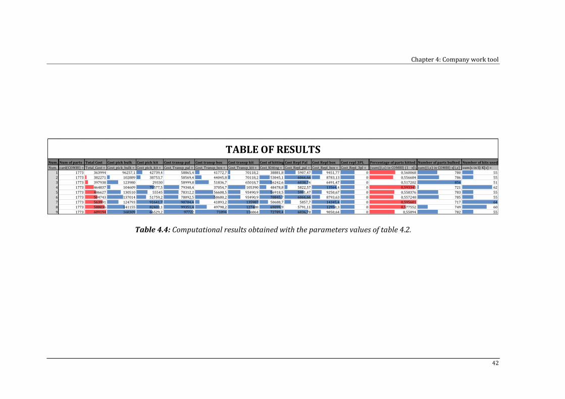
Chapter 4: Company work tool
42
Table 4.4: Computational results obtained with the parameters values of table 4.2.
Num. Num of parts Total Cost Cost pick bulk Cost pick kit Cost transp pal Cost transp box Cost transp kit Cost of kitting Cost Repl Pal Cost Repl box Cost repl 3PL Percentage of parts kitted Number of parts bulked Number of kits used
Num. card(COMBI) = Total_Cost = Cost_pick_bulk = Cost_pick_kit = Cost_Transp_pal = Cost_Transp_box = Cost_Transp_kit = Cost_Kitting = Cost_Repl_pal = Cost_Repl_box = Cost_Repl_3pl = (sum{(i,s) in COMBI} (1 - x[i,s]))/card(COMBI) =sum{(i,s) in COMBI} x[i,s] =sum{s in S} K[s] =
1 1773 363994 96257,1 42739,4 58865,4 41772,7 70118,2 38881,8 5907,47 9451,77 0 0,560068 780 55
2 1773 382271 102889 38753,7 58569,4 44045,8 70118,2 53045,1 6066,66 8783,13 0 0,556684 786 55
3 1773 397938 123980 29330 58999,8 51836,7 65018,7 56242,6 6038,74 6491,47 0 0,517202 856 51
4 1773 464837 104609 70577,5 79340,4 37054,7 105390 48478,8 5822,57 13564,4 0 0,593345 721 62
5 1773 486627 130510 55545 78312,2 56608,5 93490,9 56918,5 5991,47 9250,67 0 0,558376 783 55
6 1773 504743 137014 51759,2 78092,5 58680,2 93490,9 70845,7 6066,66 8793,63 0 0,557248 785 55
7 1773 563991 124793 91641,7 98784,4 41893,2 135987 50688,7 5857,7 14345,4 0 0,595601 717 64
8 1773 588036 141155 82403,1 99351,4 49798,2 127488 69099,9 5791,11 12950,3 0 0,577552 749 60
9 1773 609194 168309 66529,2 97722 71894 116864 72789,4 6036,78 9050,64 0 0,55894 782 55
TABLE OF RESULTS
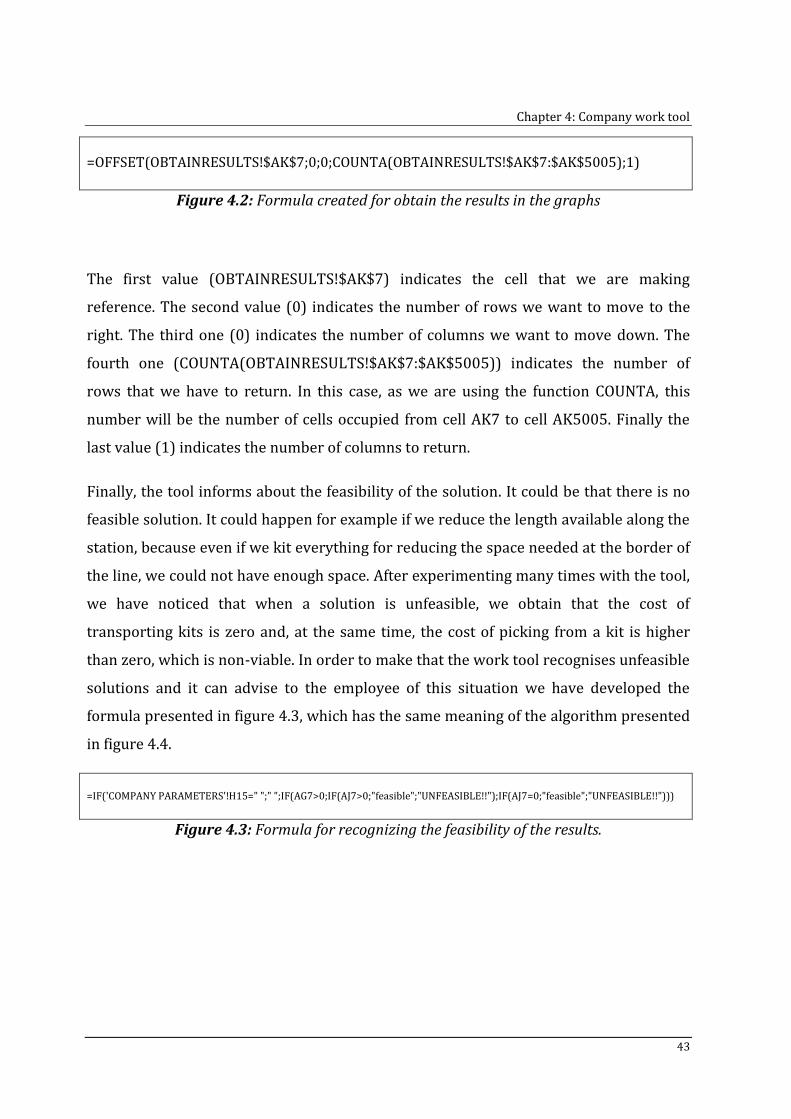
Chapter 4: Company work tool
43
=OFFSET(OBTAINRESULTS!$AK$7;0;0;COUNTA(OBTAINRESULTS!$AK$7:$AK$5005);1)
Figure 4.2: Formula created for obtain the results in the graphs
The first value (OBTAINRESULTS!$AK$7) indicates the cell that we are making
reference. The second value (0) indicates the number of rows we want to move to the
right. The third one (0) indicates the number of columns we want to move down. The
fourth one (COUNTA(OBTAINRESULTS!$AK$7:$AK$5005)) indicates the number of
rows that we have to return. In this case, as we are using the function COUNTA, this
number will be the number of cells occupied from cell AK7 to cell AK5005. Finally the
last value (1) indicates the number of columns to return.
Finally, the tool informs about the feasibility of the solution. It could be that there is no
feasible solution. It could happen for example if we reduce the length available along the
station, because even if we kit everything for reducing the space needed at the border of
the line, we could not have enough space. After experimenting many times with the tool,
we have noticed that when a solution is unfeasible, we obtain that the cost of
transporting kits is zero and, at the same time, the cost of picking from a kit is higher
than zero, which is non-viable. In order to make that the work tool recognises unfeasible
solutions and it can advise to the employee of this situation we have developed the
formula presented in figure 4.3, which has the same meaning of the algorithm presented
in figure 4.4.
=IF('COMPANY PARAMETERS'!H15=" ";" ";IF(AG7>0;IF(AJ7>0;"feasible";"UNFEASIBLE!!");IF(AJ7=0;"feasible";"UNFEASIBLE!!")))
Figure 4.3: Formula for recognizing the feasibility of the results.
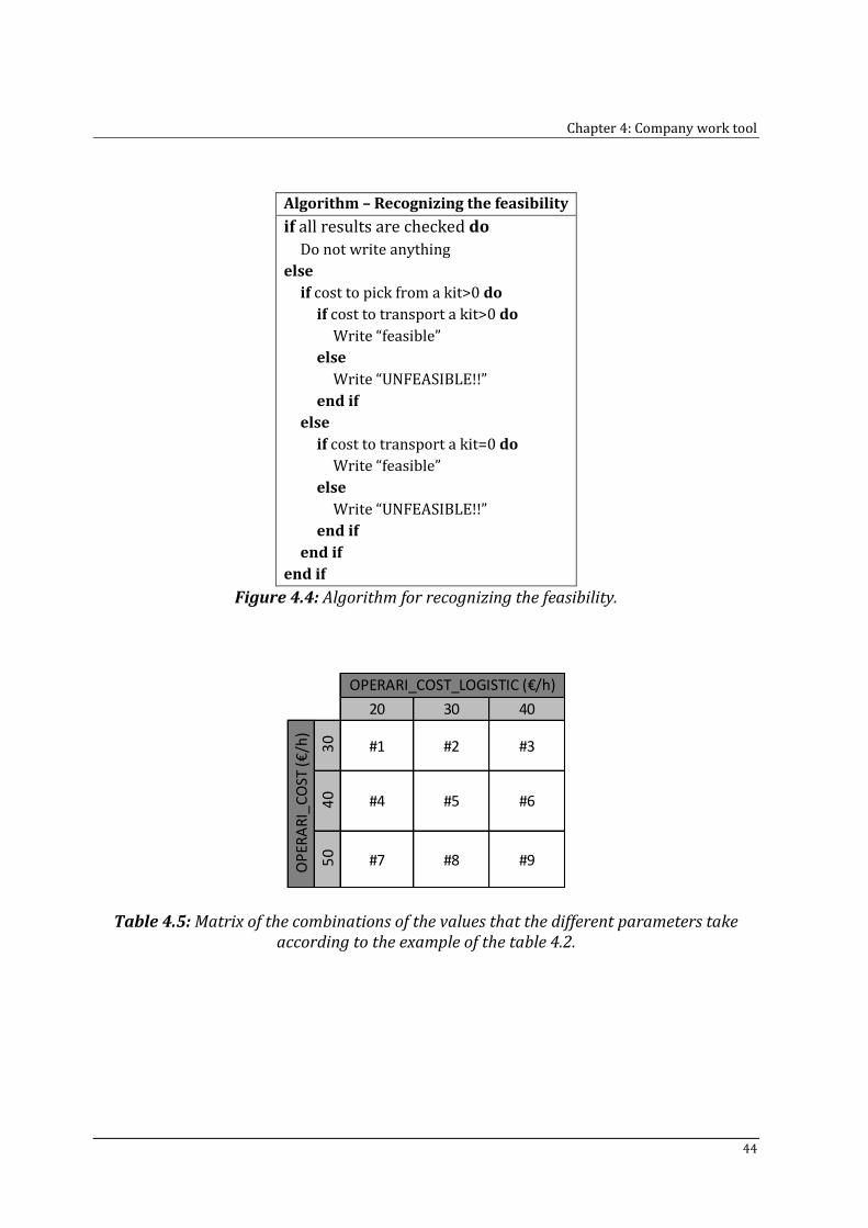
Chapter 4: Company work tool
44
Algorithm – Recognizing the feasibility
if all results are checked do
Do not write anything
else
if cost to pick from a kit>0 do
if cost to transport a kit>0 do
Write “feasible”
else
Write “UNFEASIBLE!!”
end if
else
if cost to transport a kit=0 do
Write “feasible”
else
Write “UNFEASIBLE!!”
end if
end if
end if
Figure 4.4: Algorithm for recognizing the feasibility.
Table 4.5: Matrix of the combinations of the values that the different parameters take according to the example of the table 4.2.
20 30 40
30 #1 #2 #3
40 #4 #5 #6
50 #7 #8 #9O
PER
AR
I_C
OST
(€
/h)
OPERARI_COST_LOGISTIC (€/h)
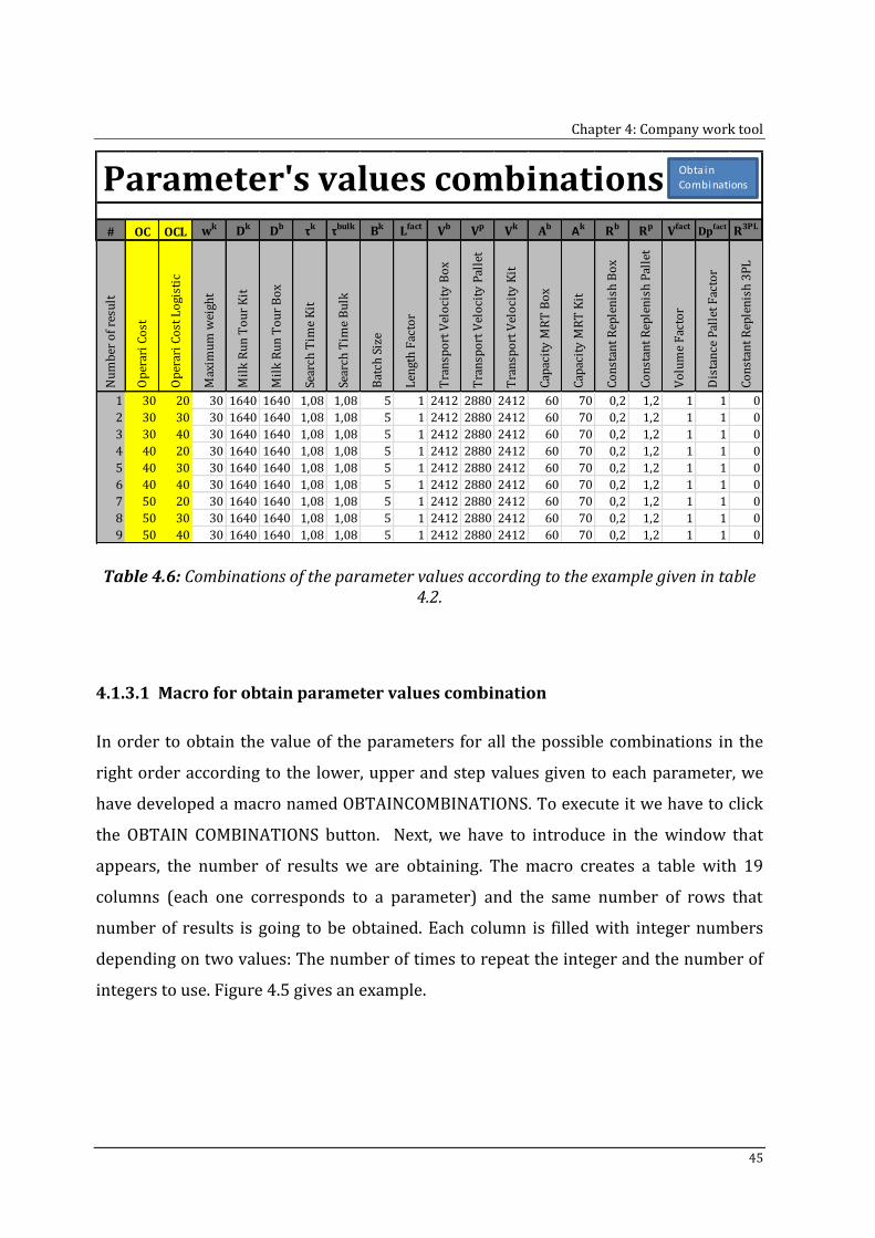
Chapter 4: Company work tool
45
Table 4.6: Combinations of the parameter values according to the example given in table 4.2.
4.1.3.1 Macro for obtain parameter values combination
In order to obtain the value of the parameters for all the possible combinations in the
right order according to the lower, upper and step values given to each parameter, we
have developed a macro named OBTAINCOMBINATIONS. To execute it we have to click
the OBTAIN COMBINATIONS button. Next, we have to introduce in the window that
appears, the number of results we are obtaining. The macro creates a table with 19
columns (each one corresponds to a parameter) and the same number of rows that
number of results is going to be obtained. Each column is filled with integer numbers
depending on two values: The number of times to repeat the integer and the number of
integers to use. Figure 4.5 gives an example.
# OC OCL wk Dk Db τk τbulk Bk Lfact Vb Vp Vk Ab Ak Rb Rp VfactDp
fact R3PL
1 30 20 30 1640 1640 1,08 1,08 5 1 2412 2880 2412 60 70 0,2 1,2 1 1 0
2 30 30 30 1640 1640 1,08 1,08 5 1 2412 2880 2412 60 70 0,2 1,2 1 1 0
3 30 40 30 1640 1640 1,08 1,08 5 1 2412 2880 2412 60 70 0,2 1,2 1 1 0
4 40 20 30 1640 1640 1,08 1,08 5 1 2412 2880 2412 60 70 0,2 1,2 1 1 0
5 40 30 30 1640 1640 1,08 1,08 5 1 2412 2880 2412 60 70 0,2 1,2 1 1 0
6 40 40 30 1640 1640 1,08 1,08 5 1 2412 2880 2412 60 70 0,2 1,2 1 1 0
7 50 20 30 1640 1640 1,08 1,08 5 1 2412 2880 2412 60 70 0,2 1,2 1 1 0
8 50 30 30 1640 1640 1,08 1,08 5 1 2412 2880 2412 60 70 0,2 1,2 1 1 0
9 50 40 30 1640 1640 1,08 1,08 5 1 2412 2880 2412 60 70 0,2 1,2 1 1 0
Parameter's values combinations
Sear
ch T
ime
Kit
Sear
ch T
ime
Bu
lk
Bat
ch S
ize
Len
gth
Fac
tor
Nu
mb
er o
f re
sult
Op
erar
i C
ost
Op
erar
i C
ost
Lo
gist
ic
Max
imu
m w
eigh
t
Mil
k R
un
To
ur
Kit
Mil
k R
un
To
ur
Bo
x
Co
nst
ant
Rep
len
ish
Pal
let
Vo
lum
e F
acto
r
Dis
tan
ce P
alle
t F
acto
r
Co
nst
ant
Rep
len
ish
3P
L
Tra
nsp
ort
Vel
oci
ty B
ox
Tra
nsp
ort
Vel
oci
ty P
alle
t
Tra
nsp
ort
Vel
oci
ty K
it
Cap
acit
y M
RT
Bo
x
Cap
acit
y M
RT
Kit
Co
nst
ant
Rep
len
ish
Bo
x
Obtain Combinations
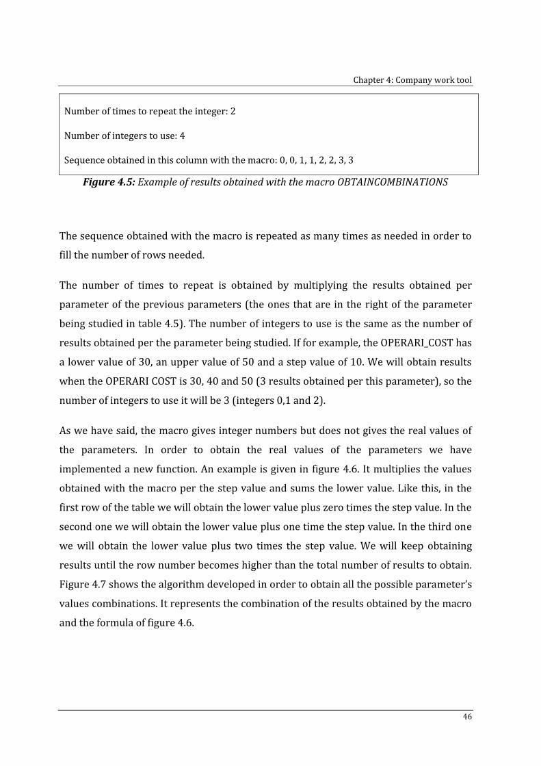
Chapter 4: Company work tool
46
Number of times to repeat the integer: 2
Number of integers to use: 4
Sequence obtained in this column with the macro: 0, 0, 1, 1, 2, 2, 3, 3
Figure 4.5: Example of results obtained with the macro OBTAINCOMBINATIONS
The sequence obtained with the macro is repeated as many times as needed in order to
fill the number of rows needed.
The number of times to repeat is obtained by multiplying the results obtained per
parameter of the previous parameters (the ones that are in the right of the parameter
being studied in table 4.5). The number of integers to use is the same as the number of
results obtained per the parameter being studied. If for example, the OPERARI_COST has
a lower value of 30, an upper value of 50 and a step value of 10. We will obtain results
when the OPERARI COST is 30, 40 and 50 (3 results obtained per this parameter), so the
number of integers to use it will be 3 (integers 0,1 and 2).
As we have said, the macro gives integer numbers but does not gives the real values of
the parameters. In order to obtain the real values of the parameters we have
implemented a new function. An example is given in figure 4.6. It multiplies the values
obtained with the macro per the step value and sums the lower value. Like this, in the
first row of the table we will obtain the lower value plus zero times the step value. In the
second one we will obtain the lower value plus one time the step value. In the third one
we will obtain the lower value plus two times the step value. We will keep obtaining
results until the row number becomes higher than the total number of results to obtain.
Figure 4.7 shows the algorithm developed in order to obtain all the possible parameter’s
values combinations. It represents the combination of the results obtained by the macro
and the formula of figure 4.6.
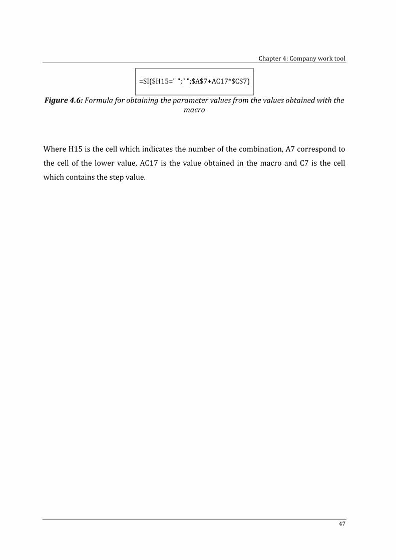
Chapter 4: Company work tool
47
=SI($H15=" ";" ";$A$7+AC17*$C$7)
Figure 4.6: Formula for obtaining the parameter values from the values obtained with the macro
Where H15 is the cell which indicates the number of the combination, A7 correspond to
the cell of the lower value, AC17 is the value obtained in the macro and C7 is the cell
which contains the step value.
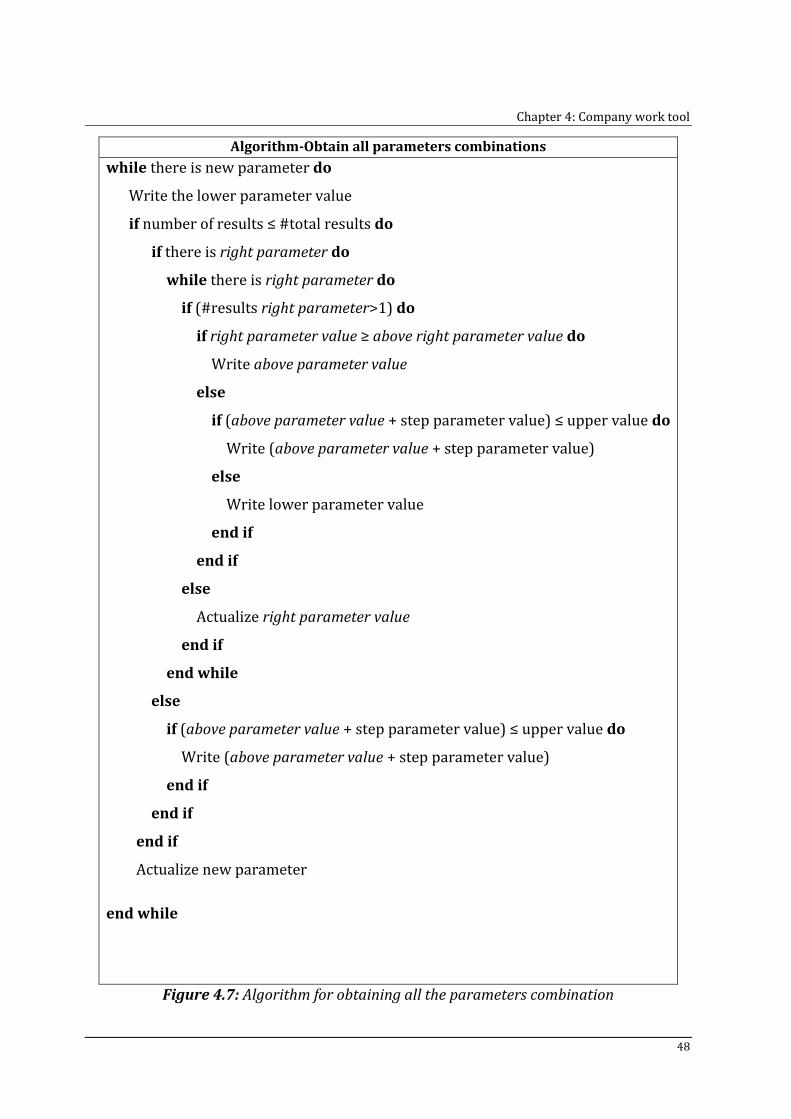
Chapter 4: Company work tool
48
Algorithm-Obtain all parameters combinations
while there is new parameter do
Write the lower parameter value
if number of results ≤ #total results do
if there is right parameter do
while there is right parameter do
if (#results right parameter>1) do
if right parameter value ≥ above right parameter value do
Write above parameter value
else
if (above parameter value + step parameter value) ≤ upper value do
Write (above parameter value + step parameter value)
else
Write lower parameter value
end if
end if
else
Actualize right parameter value
end if
end while
else
if (above parameter value + step parameter value) ≤ upper value do
Write (above parameter value + step parameter value)
end if
end if
end if
Actualize new parameter
end while
Figure 4.7: Algorithm for obtaining all the parameters combination
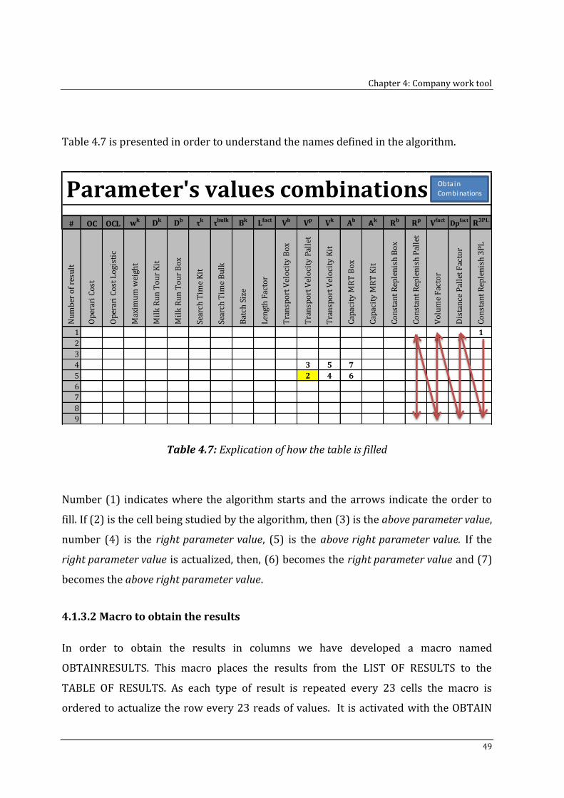
Chapter 4: Company work tool
49
Table 4.7 is presented in order to understand the names defined in the algorithm.
Table 4.7: Explication of how the table is filled
Number (1) indicates where the algorithm starts and the arrows indicate the order to
fill. If (2) is the cell being studied by the algorithm, then (3) is the above parameter value,
number (4) is the right parameter value, (5) is the above right parameter value. If the
right parameter value is actualized, then, (6) becomes the right parameter value and (7)
becomes the above right parameter value.
4.1.3.2 Macro to obtain the results
In order to obtain the results in columns we have developed a macro named
OBTAINRESULTS. This macro places the results from the LIST OF RESULTS to the
TABLE OF RESULTS. As each type of result is repeated every 23 cells the macro is
ordered to actualize the row every 23 reads of values. It is activated with the OBTAIN
# OC OCL wk Dk Db τk τbulk Bk Lfact Vb Vp Vk Ab Ak Rb Rp VfactDp
fact R3PL
1 1
2
3
4 3 5 7
5 2 4 6
6
7
8
9
Parameter's values combinationsSe
arch
Tim
e K
it
Sear
ch T
ime
Bu
lk
Bat
ch S
ize
Len
gth
Fac
tor
Nu
mb
er o
f re
sult
Op
erar
i C
ost
Op
erar
i C
ost
Lo
gist
ic
Max
imu
m w
eigh
t
Mil
k R
un
To
ur
Kit
Mil
k R
un
To
ur
Bo
x
Co
nst
ant
Rep
len
ish
Pal
let
Vo
lum
e F
acto
r
Dis
tan
ce P
alle
t F
acto
r
Co
nst
ant
Rep
len
ish
3P
L
Tra
nsp
ort
Vel
oci
ty B
ox
Tra
nsp
ort
Vel
oci
ty P
alle
t
Tra
nsp
ort
Vel
oci
ty K
it
Cap
acit
y M
RT
Bo
x
Cap
acit
y M
RT
Kit
Co
nst
ant
Rep
len
ish
Bo
x
Obtain Combinations
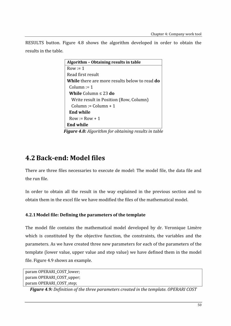
Chapter 4: Company work tool
50
RESULTS button. Figure 4.8 shows the algorithm developed in order to obtain the
results in the table.
Algorithm – Obtaining results in table
Row := 1
Read first result
While there are more results below to read do
Column := 1
While Column ≤ 23 do
Write result in Position (Row, Column)
Column := Column + 1
End while
Row := Row + 1
End while
Figure 4.8: Algorithm for obtaining results in table
4.2 Back-end: Model files
There are three files necessaries to execute de model: The model file, the data file and
the run file.
In order to obtain all the result in the way explained in the previous section and to
obtain them in the excel file we have modified the files of the mathematical model.
4.2.1 Model file: Defining the parameters of the template
The model file contains the mathematical model developed by dr. Veronique Limère
which is constituted by the objective function, the constraints, the variables and the
parameters. As we have created three new parameters for each of the parameters of the
template (lower value, upper value and step value) we have defined them in the model
file. Figure 4.9 shows an example.
param OPERARI_COST_lower;
param OPERARI_COST_upper;
param OPERARI_COST_step;
Figure 4.9: Definition of the three parameters created in the template. OPERARI COST
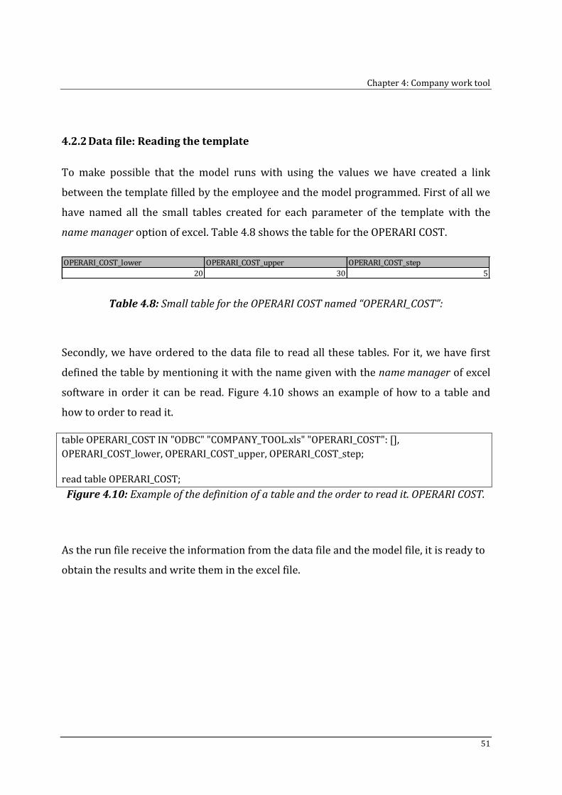
Chapter 4: Company work tool
51
4.2.2 Data file: Reading the template
To make possible that the model runs with using the values we have created a link
between the template filled by the employee and the model programmed. First of all we
have named all the small tables created for each parameter of the template with the
name manager option of excel. Table 4.8 shows the table for the OPERARI COST.
Table 4.8: Small table for the OPERARI COST named “OPERARI_COST”:
Secondly, we have ordered to the data file to read all these tables. For it, we have first
defined the table by mentioning it with the name given with the name manager of excel
software in order it can be read. Figure 4.10 shows an example of how to a table and
how to order to read it.
table OPERARI_COST IN "ODBC" "COMPANY_TOOL.xls" "OPERARI_COST": [],
OPERARI_COST_lower, OPERARI_COST_upper, OPERARI_COST_step;
read table OPERARI_COST;
Figure 4.10: Example of the definition of a table and the order to read it. OPERARI COST.
As the run file receive the information from the data file and the model file, it is ready to
obtain the results and write them in the excel file.
OPERARI_COST_lower OPERARI_COST_upper OPERARI_COST_step
20 30 5
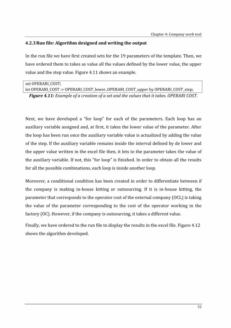
Chapter 4: Company work tool
52
4.2.3 Run file: Algorithm designed and writing the output
In the run file we have first created sets for the 19 parameters of the template. Then, we
have ordered them to takes as value all the values defined by the lower value, the upper
value and the step value. Figure 4.11 shows an example.
set OPERARI_COST;
let OPERARI_COST := OPERARI_COST_lower..OPERARI_COST_upper by OPERARI_COST_step;
Figure 4.11: Example of a creation of a set and the values that it takes. OPERARI COST.
Next, we have developed a “for loop” for each of the parameters. Each loop has an
auxiliary variable assigned and, at first, it takes the lower value of the parameter. After
the loop has been run once the auxiliary variable value is actualized by adding the value
of the step. If the auxiliary variable remains inside the interval defined by de lower and
the upper value written in the excel file then, it lets to the parameter takes the value of
the auxiliary variable. If not, this “for loop” is finished. In order to obtain all the results
for all the possible combinations, each loop is inside another loop.
Moreover, a conditional condition has been created in order to differentiate between if
the company is making in-house kitting or outsourcing. If it is in-house kitting, the
parameter that corresponds to the operator cost of the external company (OCL) is taking
the value of the parameter corresponding to the cost of the operator working in the
factory (OC). However, if the company is outsourcing, it takes a different value.
Finally, we have ordered to the run file to display the results in the excel file. Figure 4.12
shows the algorithm developed.
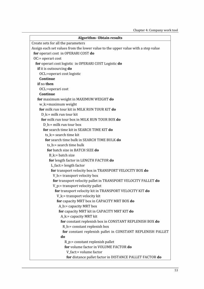
Chapter 4: Company work tool
53
Algorithm- Obtain results
Create sets for all the parameters
Assign each set values from the lower value to the upper value with a step value
for operari cost in OPERARI COST do
OC:= operari cost
for operari cost logistic in OPERARI COST Logistic do
if it is outsourcing do
OCL:=operari cost logistic
Continue
if no then
OCL:=operari cost
Continue
for maximum weight in MAXIMUM WEIGHT do
w_k:=maximum weight
for milk run tour kit in MILK RUN TOUR KIT do
D_k:= milk run tour kit
for milk run tour box in MILK RUN TOUR BOX do
D_b:= milk run tour box
for search time kit in SEARCH TIME KIT do
ts_k:= search time kit
for search time bulk in SEARCH TIME BULK do
ts_b:= search time bulk
for batch size in BATCH SIZE do
B_k:= batch size
for length factor in LENGTH FACTOR do
L_fact:= length factor
for transport velocity box in TRANSPORT VELOCITY BOX do
V_b:= transport velocity box
for transport velocity pallet in TRANSPORT VELOCITY PALLET do
V_p:= transport velocity pallet
for transport velocity kit in TRANSPORT VELOCITY KIT do
V_k:= transport velocity kit
for capacity MRT box in CAPACITY MRT BOX do
A_b:= capacity MRT box
for capacity MRT kit in CAPACITY MRT KIT do
A_k:= capacity MRT kit
for constant replenish box in CONSTANT REPLENISH BOX do
R_b:= constant replenish box
for constant replenish pallet in CONSTANT REPLENISH PALLET
do
R_p:= constant replenish pallet
for volume factor in VOLUME FACTOR do
V_fact:= volume factor
for distance pallet factor in DISTANCE PALLET FACTOR do
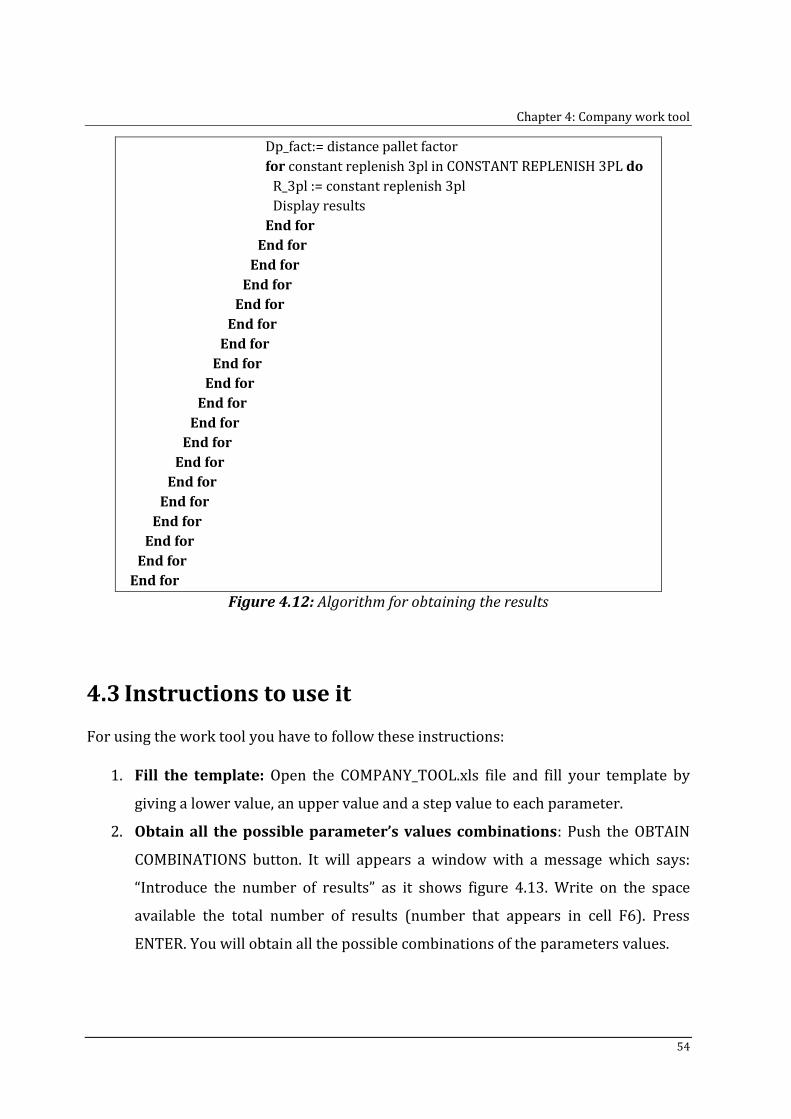
Chapter 4: Company work tool
54
Dp_fact:= distance pallet factor
for constant replenish 3pl in CONSTANT REPLENISH 3PL do
R_3pl := constant replenish 3pl
Display results
End for
End for
End for
End for
End for
End for
End for
End for
End for
End for
End for
End for
End for
End for
End for
End for
End for
End for
End for
Figure 4.12: Algorithm for obtaining the results
4.3 Instructions to use it
For using the work tool you have to follow these instructions:
1. Fill the template: Open the COMPANY_TOOL.xls file and fill your template by
giving a lower value, an upper value and a step value to each parameter.
2. Obtain all the possible parameter’s values combinations: Push the OBTAIN
COMBINATIONS button. It will appears a window with a message which says:
“Introduce the number of results” as it shows figure 4.13. Write on the space
available the total number of results (number that appears in cell F6). Press
ENTER. You will obtain all the possible combinations of the parameters values.
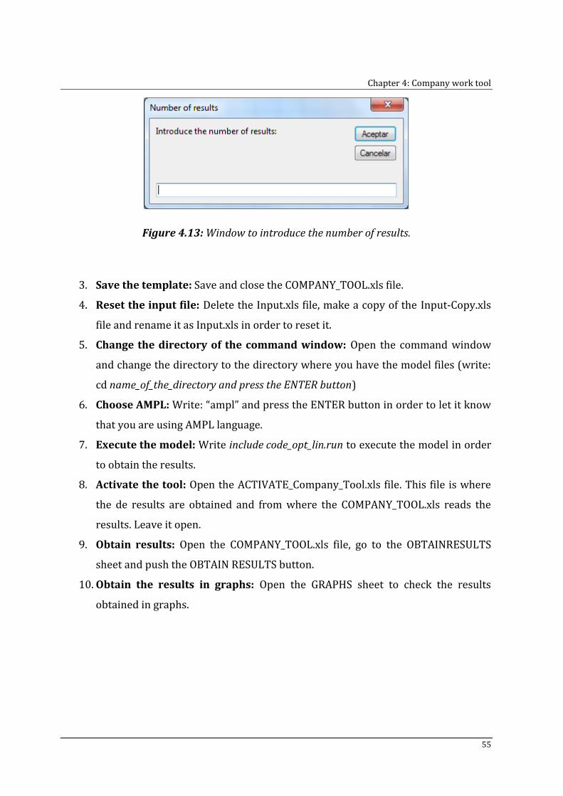
Chapter 4: Company work tool
55
Figure 4.13: Window to introduce the number of results.
3. Save the template: Save and close the COMPANY_TOOL.xls file.
4. Reset the input file: Delete the Input.xls file, make a copy of the Input-Copy.xls
file and rename it as Input.xls in order to reset it.
5. Change the directory of the command window: Open the command window
and change the directory to the directory where you have the model files (write:
cd name_of_the_directory and press the ENTER button)
6. Choose AMPL: Write: “ampl” and press the ENTER button in order to let it know
that you are using AMPL language.
7. Execute the model: Write include code_opt_lin.run to execute the model in order
to obtain the results.
8. Activate the tool: Open the ACTIVATE_Company_Tool.xls file. This file is where
the de results are obtained and from where the COMPANY_TOOL.xls reads the
results. Leave it open.
9. Obtain results: Open the COMPANY_TOOL.xls file, go to the OBTAINRESULTS
sheet and push the OBTAIN RESULTS button.
10. Obtain the results in graphs: Open the GRAPHS sheet to check the results
obtained in graphs.
Chapter 5
Computational results
In this chapter are presented all the computational results of the considerations made in
Chapter 3. After having developed the work tool, we are going to use it to be able to
analyse the impact that the possible changes in the supply chain has to the final cost. We
will also analyse if it repercutes on the percentage of parts kitted. All the results are
obtained from a particular input data. It means that, if another company is using the tool,
results will vary according to their type of parts. In this particular case, if we consider
that parameters are taking the values of the thesis “To kit or not to kit: Optimizing part
feeding in the Automotive Assembly Industry” by dr. Veronique Limère (Table 5.1), the
results obtained are the ones that are shown in table 5.2.
In the following sections, different studies are realized in order to analyse the impact of
the parameter’s values in the costs and in the percentage of parts kitted.
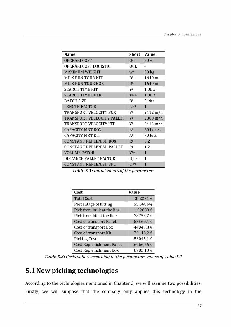
Chapter 6: Conclusions
57
Name Short Value
OPERARI COST OC 30 €
OPERARI COST LOGISTIC OCL -
MAXIMUM WEIGHT wk 30 kg
MILK RUN TOUR KIT Dk 1640 m
MILK RUN TOUR BOX Db 1640 m
SEARCH TIME KIT τk 1,08 s
SEARCH TIME BULK τbulk 1,08 s
BATCH SIZE Bk 5 kits
LENGTH FACTOR Lfact 1
TRANSPORT VELOCITY BOX Vb 2412 m/h
TRANSPORT VELLOCITY PALLET Vp 2880 m/h
TRANSPORT VELOCITY KIT Vk 2412 m/h
CAPACITY MRT BOX Ab 60 boxes
CAPACITY MRT KIT Ak 70 kits
CONSTANT REPLENISH BOX Rb 0,2
CONSTANT REPLENISH PALLET Rp 1,2
VOLUME FATOR Vfact 1
DISTANCE PALLET FACTOR Dpfact 1
CONSTANT REPLENISH 3PL C3PL 1
Table 5.1: Initial values of the parameters
Cost Value
Total Cost 382271 €
Percentage of kitting 55,6684%
Pick from bulk at the line 102889 €
Pick from kit at the line 38753,7 €
Cost of transport Pallet 58569,4 €
Cost of transport Box 44045,8 €
Cost of transport Kit 70118,2 €
Picking Cost 53045,1 €
Cost Replenishment Pallet 6066,66 €
Cost Replenishment Box 8783,13 €
Table 5.2: Costs values according to the parameters values of Table 5.1
5.1 New picking technologies
According to the technologies mentioned in Chapter 3, we will assume two possibilities.
Firstly, we will suppose that the company only applies this technology in the
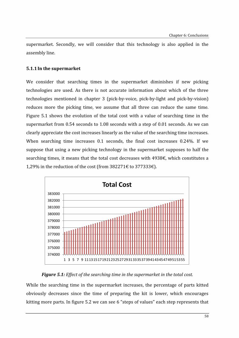
Chapter 6: Conclusions
58
supermarket. Secondly, we will consider that this technology is also applied in the
assembly line.
5.1.1 In the supermarket
We consider that searching times in the supermarket diminishes if new picking
technologies are used. As there is not accurate information about which of the three
technologies mentioned in chapter 3 (pick-by-voice, pick-by-light and pick-by-vision)
reduces more the picking time, we assume that all three can reduce the same time.
Figure 5.1 shows the evolution of the total cost with a value of searching time in the
supermarket from 0.54 seconds to 1.08 seconds with a step of 0.01 seconds. As we can
clearly appreciate the cost increases linearly as the value of the searching time increases.
When searching time increases 0.1 seconds, the final cost increases 0.24%. If we
suppose that using a new picking technology in the supermarket supposes to half the
searching times, it means that the total cost decreases with 4938€, which constitutes a
1,29% in the reduction of the cost (from 382271€ to 377333€).
Figure 5.1: Effect of the searching time in the supermarket in the total cost.
While the searching time in the supermarket increases, the percentage of parts kitted
obviously decreases since the time of preparing the kit is lower, which encourages
kitting more parts. In figure 5.2 we can see 6 “steps of values” each step represents that
374000
375000
376000
377000
378000
379000
380000
381000
382000
383000
1 3 5 7 9 1113151719212325272931333537394143454749515355
Total Cost
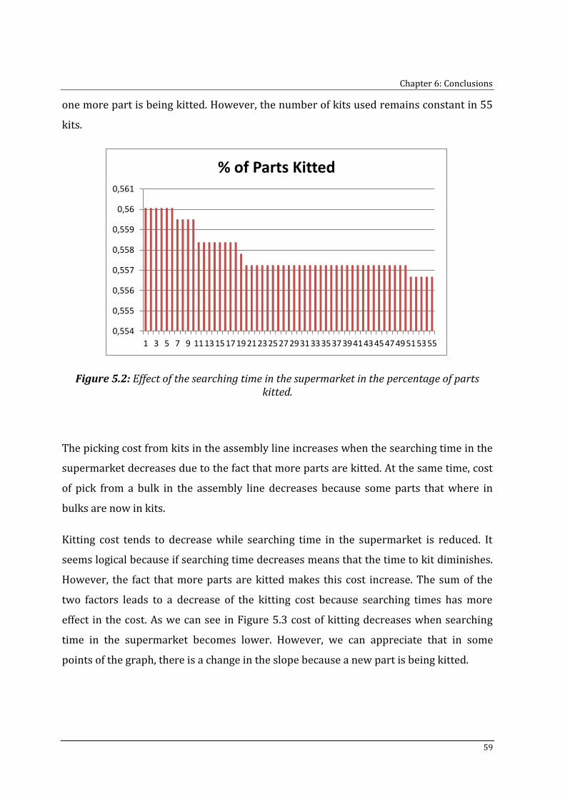
Chapter 6: Conclusions
59
one more part is being kitted. However, the number of kits used remains constant in 55
kits.
Figure 5.2: Effect of the searching time in the supermarket in the percentage of parts kitted.
The picking cost from kits in the assembly line increases when the searching time in the
supermarket decreases due to the fact that more parts are kitted. At the same time, cost
of pick from a bulk in the assembly line decreases because some parts that where in
bulks are now in kits.
Kitting cost tends to decrease while searching time in the supermarket is reduced. It
seems logical because if searching time decreases means that the time to kit diminishes.
However, the fact that more parts are kitted makes this cost increase. The sum of the
two factors leads to a decrease of the kitting cost because searching times has more
effect in the cost. As we can see in Figure 5.3 cost of kitting decreases when searching
time in the supermarket becomes lower. However, we can appreciate that in some
points of the graph, there is a change in the slope because a new part is being kitted.
0,554
0,555
0,556
0,557
0,558
0,559
0,56
0,561
1 3 5 7 9 1113151719212325272931333537394143454749515355
% of Parts Kitted
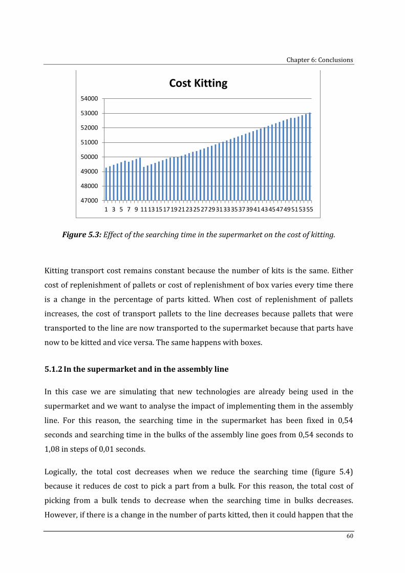
Chapter 6: Conclusions
60
Figure 5.3: Effect of the searching time in the supermarket on the cost of kitting.
Kitting transport cost remains constant because the number of kits is the same. Either
cost of replenishment of pallets or cost of replenishment of box varies every time there
is a change in the percentage of parts kitted. When cost of replenishment of pallets
increases, the cost of transport pallets to the line decreases because pallets that were
transported to the line are now transported to the supermarket because that parts have
now to be kitted and vice versa. The same happens with boxes.
5.1.2 In the supermarket and in the assembly line
In this case we are simulating that new technologies are already being used in the
supermarket and we want to analyse the impact of implementing them in the assembly
line. For this reason, the searching time in the supermarket has been fixed in 0,54
seconds and searching time in the bulks of the assembly line goes from 0,54 seconds to
1,08 in steps of 0,01 seconds.
Logically, the total cost decreases when we reduce the searching time (figure 5.4)
because it reduces de cost to pick a part from a bulk. For this reason, the total cost of
picking from a bulk tends to decrease when the searching time in bulks decreases.
However, if there is a change in the number of parts kitted, then it could happen that the
47000
48000
49000
50000
51000
52000
53000
54000
1 3 5 7 9 1113151719212325272931333537394143454749515355
Cost Kitting
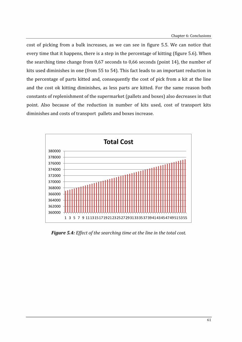
Chapter 6: Conclusions
61
cost of picking from a bulk increases, as we can see in figure 5.5. We can notice that
every time that it happens, there is a step in the percentage of kitting (figure 5.6). When
the searching time change from 0,67 seconds to 0,66 seconds (point 14), the number of
kits used diminishes in one (from 55 to 54). This fact leads to an important reduction in
the percentage of parts kitted and, consequently the cost of pick from a kit at the line
and the cost ok kitting diminishes, as less parts are kitted. For the same reason both
constants of replenishment of the supermarket (pallets and boxes) also decreases in that
point. Also because of the reduction in number of kits used, cost of transport kits
diminishes and costs of transport pallets and boxes increase.
Figure 5.4: Effect of the searching time at the line in the total cost.
360000
362000
364000
366000
368000
370000
372000
374000
376000
378000
380000
1 3 5 7 9 1113151719212325272931333537394143454749515355
Total Cost
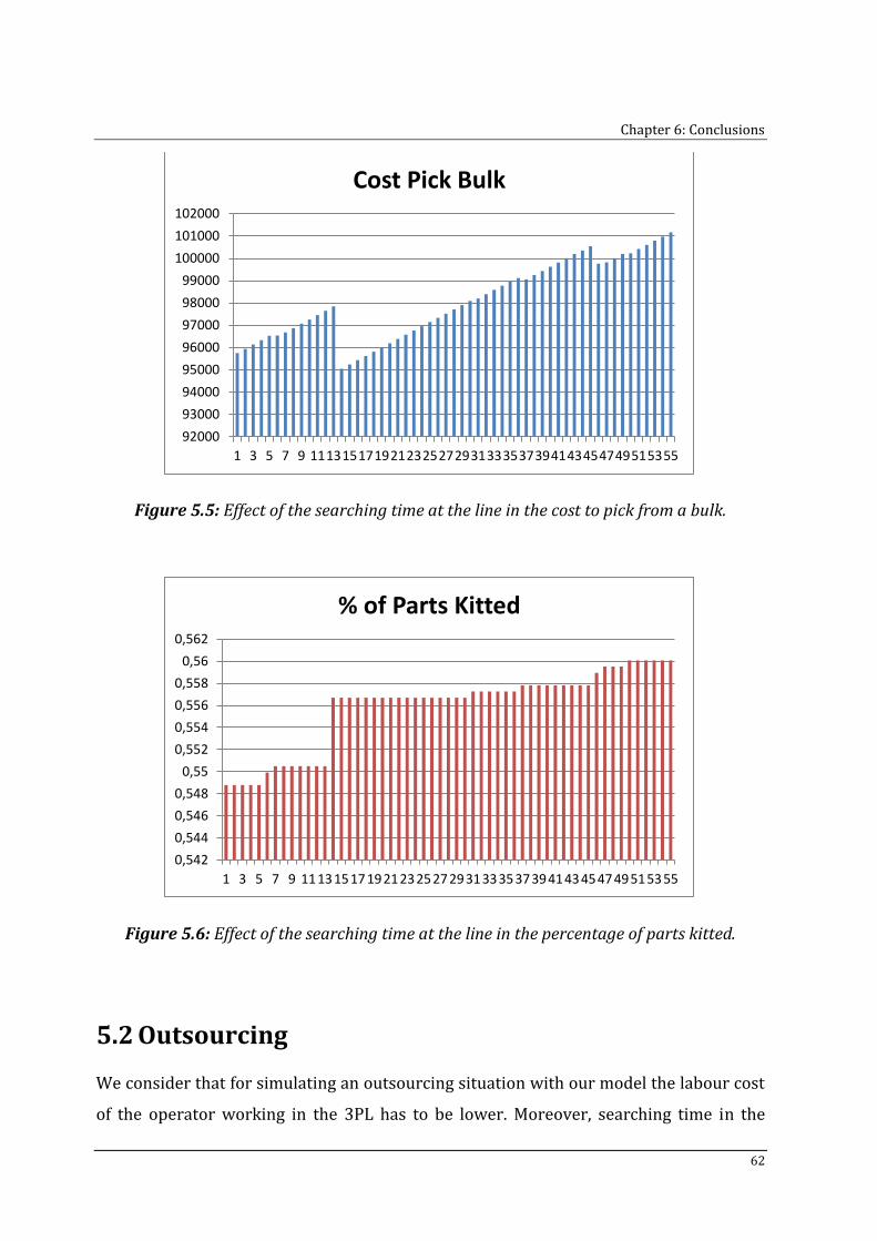
Chapter 6: Conclusions
62
Figure 5.5: Effect of the searching time at the line in the cost to pick from a bulk.
Figure 5.6: Effect of the searching time at the line in the percentage of parts kitted.
5.2 Outsourcing
We consider that for simulating an outsourcing situation with our model the labour cost
of the operator working in the 3PL has to be lower. Moreover, searching time in the
92000
93000
94000
95000
96000
97000
98000
99000
100000
101000
102000
1 3 5 7 9 1113151719212325272931333537394143454749515355
Cost Pick Bulk
0,542
0,544
0,546
0,548
0,55
0,552
0,554
0,556
0,558
0,56
0,562
1 3 5 7 9 1113151719212325272931333537394143454749515355
% of Parts Kitted
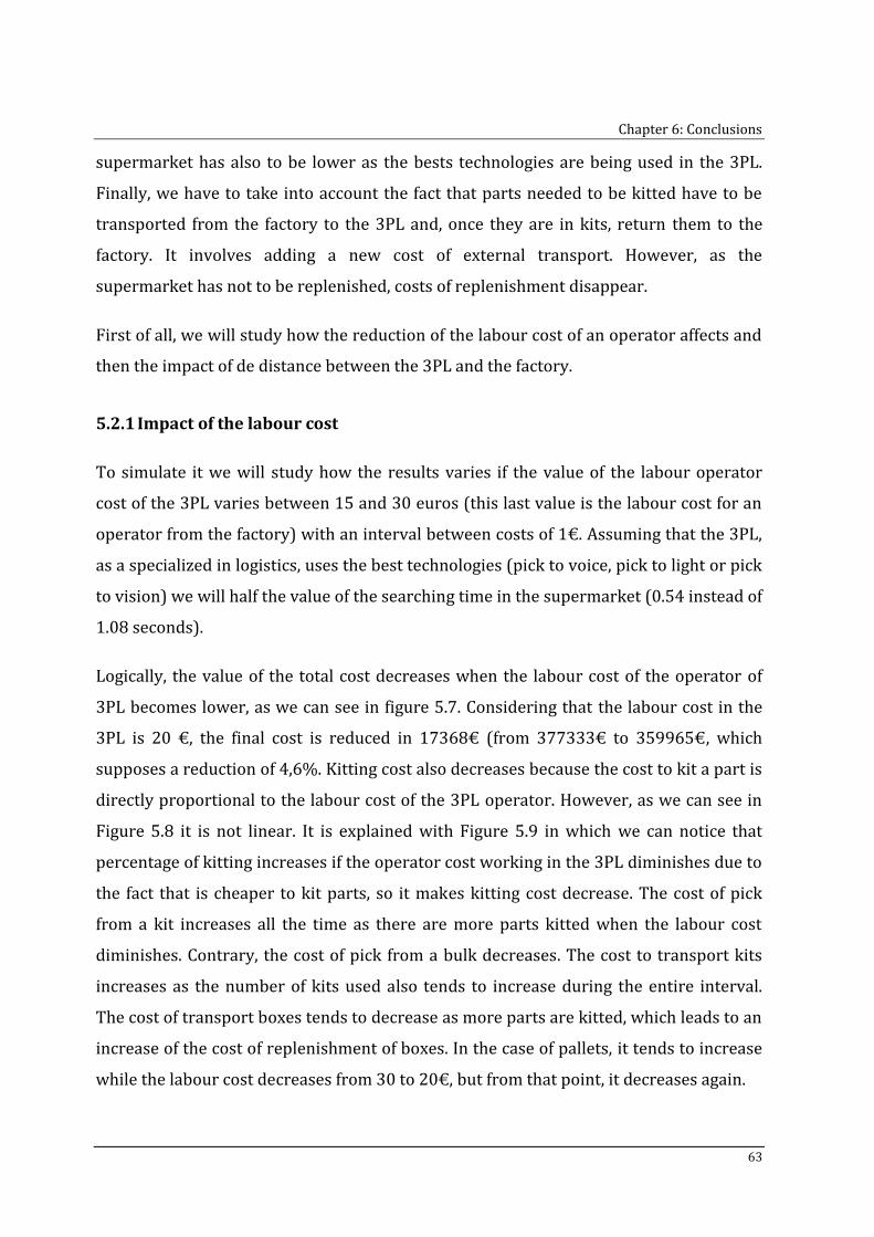
Chapter 6: Conclusions
63
supermarket has also to be lower as the bests technologies are being used in the 3PL.
Finally, we have to take into account the fact that parts needed to be kitted have to be
transported from the factory to the 3PL and, once they are in kits, return them to the
factory. It involves adding a new cost of external transport. However, as the
supermarket has not to be replenished, costs of replenishment disappear.
First of all, we will study how the reduction of the labour cost of an operator affects and
then the impact of de distance between the 3PL and the factory.
5.2.1 Impact of the labour cost
To simulate it we will study how the results varies if the value of the labour operator
cost of the 3PL varies between 15 and 30 euros (this last value is the labour cost for an
operator from the factory) with an interval between costs of 1€. Assuming that the 3PL,
as a specialized in logistics, uses the best technologies (pick to voice, pick to light or pick
to vision) we will half the value of the searching time in the supermarket (0.54 instead of
1.08 seconds).
Logically, the value of the total cost decreases when the labour cost of the operator of
3PL becomes lower, as we can see in figure 5.7. Considering that the labour cost in the
3PL is 20 €, the final cost is reduced in 17368€ (from 377333€ to 359965€, which
supposes a reduction of 4,6%. Kitting cost also decreases because the cost to kit a part is
directly proportional to the labour cost of the 3PL operator. However, as we can see in
Figure 5.8 it is not linear. It is explained with Figure 5.9 in which we can notice that
percentage of kitting increases if the operator cost working in the 3PL diminishes due to
the fact that is cheaper to kit parts, so it makes kitting cost decrease. The cost of pick
from a kit increases all the time as there are more parts kitted when the labour cost
diminishes. Contrary, the cost of pick from a bulk decreases. The cost to transport kits
increases as the number of kits used also tends to increase during the entire interval.
The cost of transport boxes tends to decrease as more parts are kitted, which leads to an
increase of the cost of replenishment of boxes. In the case of pallets, it tends to increase
while the labour cost decreases from 30 to 20€, but from that point, it decreases again.
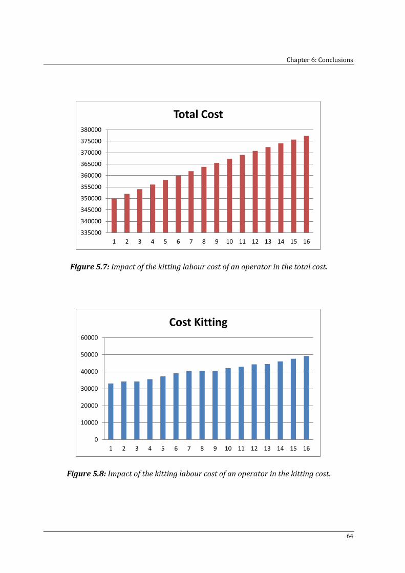
Chapter 6: Conclusions
64
Figure 5.7: Impact of the kitting labour cost of an operator in the total cost.
Figure 5.8: Impact of the kitting labour cost of an operator in the kitting cost.
335000
340000
345000
350000
355000
360000
365000
370000
375000
380000
1 2 3 4 5 6 7 8 9 10 11 12 13 14 15 16
Total Cost
0
10000
20000
30000
40000
50000
60000
1 2 3 4 5 6 7 8 9 10 11 12 13 14 15 16
Cost Kitting
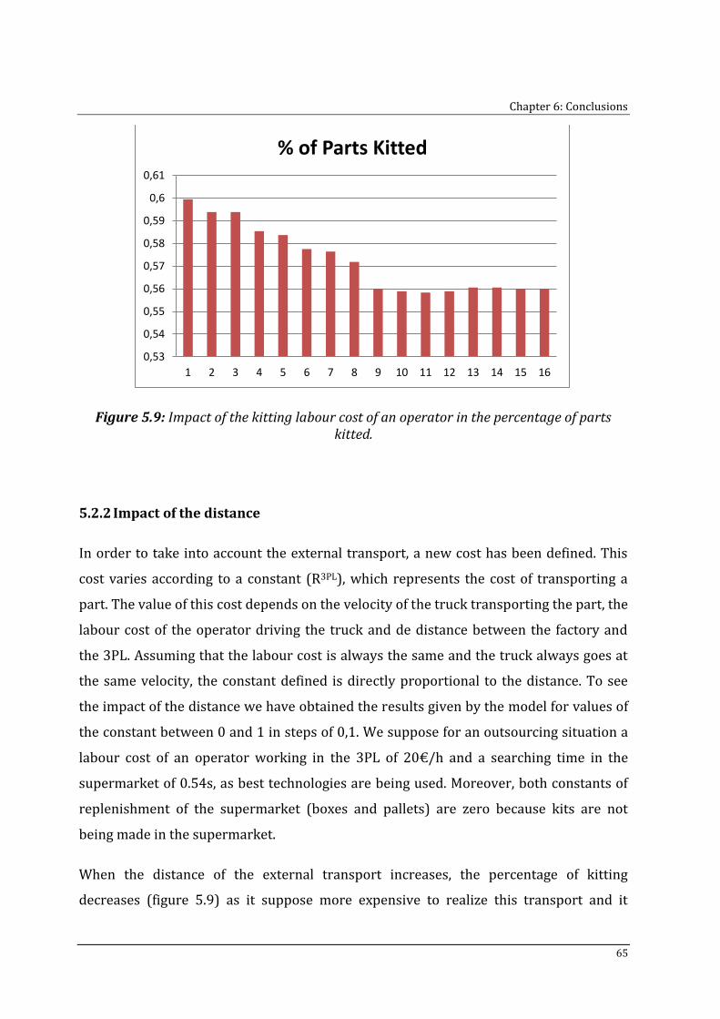
Chapter 6: Conclusions
65
Figure 5.9: Impact of the kitting labour cost of an operator in the percentage of parts kitted.
5.2.2 Impact of the distance
In order to take into account the external transport, a new cost has been defined. This
cost varies according to a constant (R3PL), which represents the cost of transporting a
part. The value of this cost depends on the velocity of the truck transporting the part, the
labour cost of the operator driving the truck and de distance between the factory and
the 3PL. Assuming that the labour cost is always the same and the truck always goes at
the same velocity, the constant defined is directly proportional to the distance. To see
the impact of the distance we have obtained the results given by the model for values of
the constant between 0 and 1 in steps of 0,1. We suppose for an outsourcing situation a
labour cost of an operator working in the 3PL of 20€/h and a searching time in the
supermarket of 0.54s, as best technologies are being used. Moreover, both constants of
replenishment of the supermarket (boxes and pallets) are zero because kits are not
being made in the supermarket.
When the distance of the external transport increases, the percentage of kitting
decreases (figure 5.9) as it suppose more expensive to realize this transport and it
0,53
0,54
0,55
0,56
0,57
0,58
0,59
0,6
0,61
1 2 3 4 5 6 7 8 9 10 11 12 13 14 15 16
% of Parts Kitted
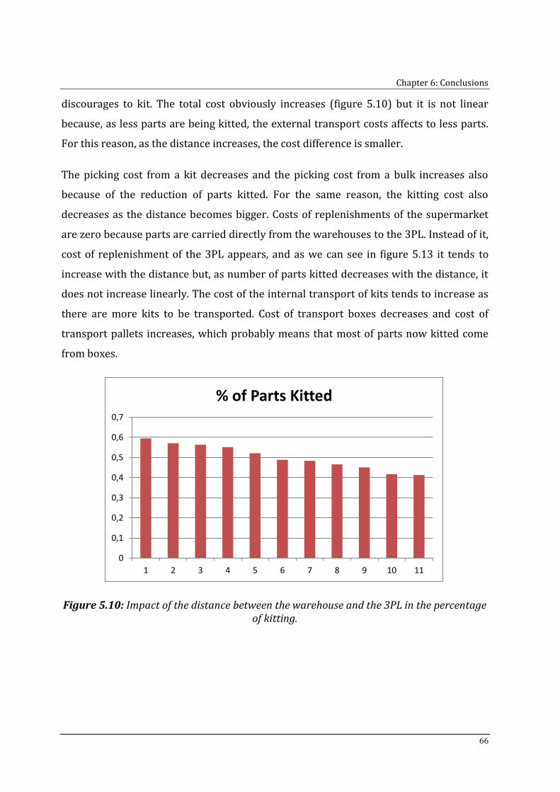
Chapter 6: Conclusions
66
discourages to kit. The total cost obviously increases (figure 5.10) but it is not linear
because, as less parts are being kitted, the external transport costs affects to less parts.
For this reason, as the distance increases, the cost difference is smaller.
The picking cost from a kit decreases and the picking cost from a bulk increases also
because of the reduction of parts kitted. For the same reason, the kitting cost also
decreases as the distance becomes bigger. Costs of replenishments of the supermarket
are zero because parts are carried directly from the warehouses to the 3PL. Instead of it,
cost of replenishment of the 3PL appears, and as we can see in figure 5.13 it tends to
increase with the distance but, as number of parts kitted decreases with the distance, it
does not increase linearly. The cost of the internal transport of kits tends to increase as
there are more kits to be transported. Cost of transport boxes decreases and cost of
transport pallets increases, which probably means that most of parts now kitted come
from boxes.
Figure 5.10: Impact of the distance between the warehouse and the 3PL in the percentage of kitting.
0
0,1
0,2
0,3
0,4
0,5
0,6
0,7
1 2 3 4 5 6 7 8 9 10 11
% of Parts Kitted
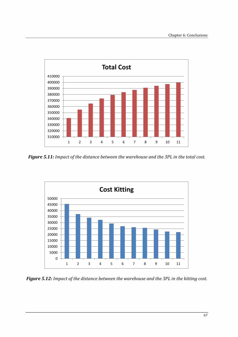
Chapter 6: Conclusions
67
Figure 5.11: Impact of the distance between the warehouse and the 3PL in the total cost.
Figure 5.12: Impact of the distance between the warehouse and the 3PL in the kitting cost.
310000
320000
330000
340000
350000
360000
370000
380000
390000
400000
410000
1 2 3 4 5 6 7 8 9 10 11
Total Cost
0
5000
10000
15000
20000
25000
30000
35000
40000
45000
50000
1 2 3 4 5 6 7 8 9 10 11
Cost Kitting
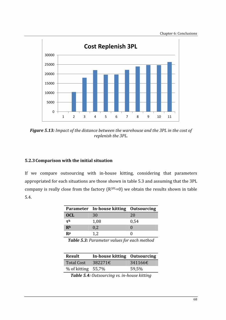
Chapter 6: Conclusions
68
Figure 5.13: Impact of the distance between the warehouse and the 3PL in the cost of replenish the 3PL.
5.2.3 Comparison with the initial situation
If we compare outsourcing with in-house kitting, considering that parameters
appropriated for each situations are those shown in table 5.3 and assuming that the 3PL
company is really close from the factory (R3PL=0) we obtain the results shown in table
5.4.
Parameter In-house kitting Outsourcing
OCL 30 20
τk 1,08 0,54
Rb 0,2 0
Rp 1,2 0
Table 5.3: Parameter values for each method
Result In-house kitting Outsourcing
Total Cost 382271€ 341166€
% of kitting 55,7% 59,5%
Table 5.4: Outsourcing vs. in-house kitting
0
5000
10000
15000
20000
25000
30000
1 2 3 4 5 6 7 8 9 10 11
Cost Replenish 3PL
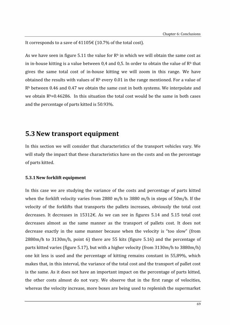
Chapter 6: Conclusions
69
It corresponds to a save of 41105€ (10.7% of the total cost).
As we have seen in figure 5.11 the value for Rb in which we will obtain the same cost as
in in-house kitting is a value between 0,4 and 0,5. In order to obtain the value of Rb that
gives the same total cost of in-house kitting we will zoom in this range. We have
obtained the results with values of Rb every 0.01 in the range mentioned. For a value of
Rb between 0.46 and 0.47 we obtain the same cost in both systems. We interpolate and
we obtain Rb=0.46286. In this situation the total cost would be the same in both cases
and the percentage of parts kitted is 50.93%.
5.3 New transport equipment
In this section we will consider that characteristics of the transport vehicles vary. We
will study the impact that these characteristics have on the costs and on the percentage
of parts kitted.
5.3.1 New forklift equipment
In this case we are studying the variance of the costs and percentage of parts kitted
when the forklift velocity varies from 2880 m/h to 3880 m/h in steps of 50m/h. If the
velocity of the forklifts that transports the pallets increases, obviously the total cost
decreases. It decreases in 15312€. As we can see in figures 5.14 and 5.15 total cost
decreases almost as the same manner as the transport of pallets cost. It does not
decrease exactly in the same manner because when the velocity is “too slow” (from
2880m/h to 3130m/h, point 6) there are 55 kits (figure 5.16) and the percentage of
parts kitted varies (figure 5.17), but with a higher velocity (from 3130m/h to 3880m/h)
one kit less is used and the percentage of kitting remains constant in 55,89%, which
makes that, in this interval, the variance of the total cost and the transport of pallet cost
is the same. As it does not have an important impact on the percentage of parts kitted,
the other costs almost do not vary. We observe that in the first range of velocities,
whereas the velocity increase, more boxes are being used to replenish the supermarket
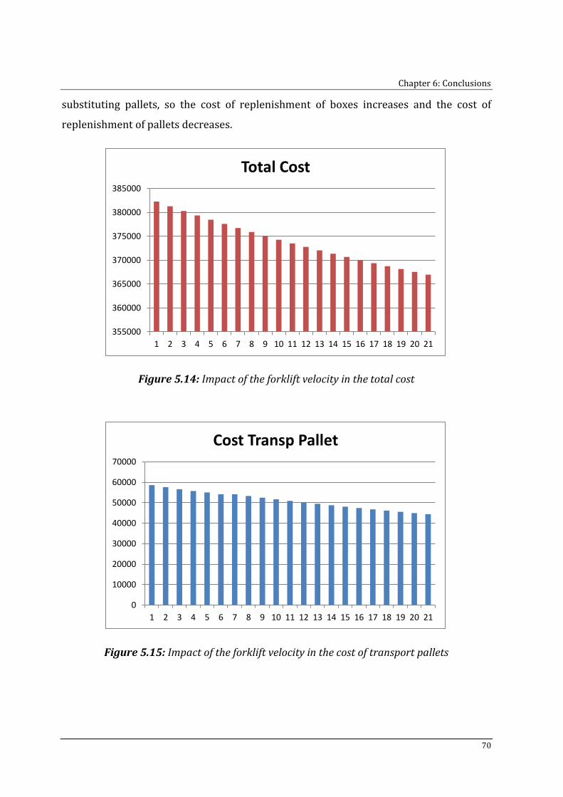
Chapter 6: Conclusions
70
substituting pallets, so the cost of replenishment of boxes increases and the cost of
replenishment of pallets decreases.
Figure 5.14: Impact of the forklift velocity in the total cost
Figure 5.15: Impact of the forklift velocity in the cost of transport pallets
355000
360000
365000
370000
375000
380000
385000
1 2 3 4 5 6 7 8 9 10 11 12 13 14 15 16 17 18 19 20 21
Total Cost
0
10000
20000
30000
40000
50000
60000
70000
1 2 3 4 5 6 7 8 9 10 11 12 13 14 15 16 17 18 19 20 21
Cost Transp Pallet
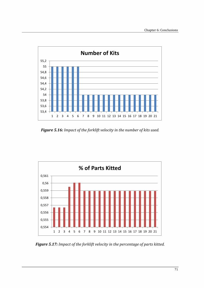
Chapter 6: Conclusions
71
Figure 5.16: Impact of the forklift velocity in the number of kits used.
Figure 5.17: Impact of the forklift velocity in the percentage of parts kitted.
53,4
53,6
53,8
54
54,2
54,4
54,6
54,8
55
55,2
1 2 3 4 5 6 7 8 9 10 11 12 13 14 15 16 17 18 19 20 21
Number of Kits
0,554
0,555
0,556
0,557
0,558
0,559
0,56
0,561
1 2 3 4 5 6 7 8 9 10 11 12 13 14 15 16 17 18 19 20 21
% of Parts Kitted
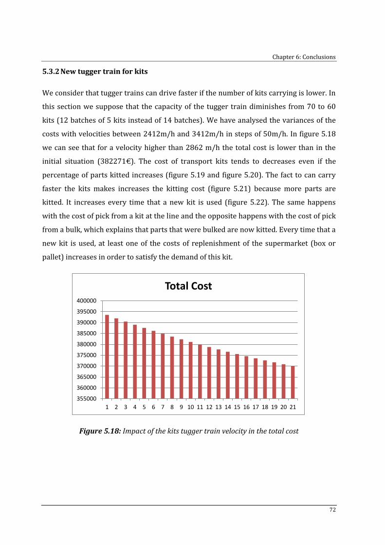
Chapter 6: Conclusions
72
5.3.2 New tugger train for kits
We consider that tugger trains can drive faster if the number of kits carrying is lower. In
this section we suppose that the capacity of the tugger train diminishes from 70 to 60
kits (12 batches of 5 kits instead of 14 batches). We have analysed the variances of the
costs with velocities between 2412m/h and 3412m/h in steps of 50m/h. In figure 5.18
we can see that for a velocity higher than 2862 m/h the total cost is lower than in the
initial situation (382271€). The cost of transport kits tends to decreases even if the
percentage of parts kitted increases (figure 5.19 and figure 5.20). The fact to can carry
faster the kits makes increases the kitting cost (figure 5.21) because more parts are
kitted. It increases every time that a new kit is used (figure 5.22). The same happens
with the cost of pick from a kit at the line and the opposite happens with the cost of pick
from a bulk, which explains that parts that were bulked are now kitted. Every time that a
new kit is used, at least one of the costs of replenishment of the supermarket (box or
pallet) increases in order to satisfy the demand of this kit.
Figure 5.18: Impact of the kits tugger train velocity in the total cost
355000
360000
365000
370000
375000
380000
385000
390000
395000
400000
1 2 3 4 5 6 7 8 9 10 11 12 13 14 15 16 17 18 19 20 21
Total Cost
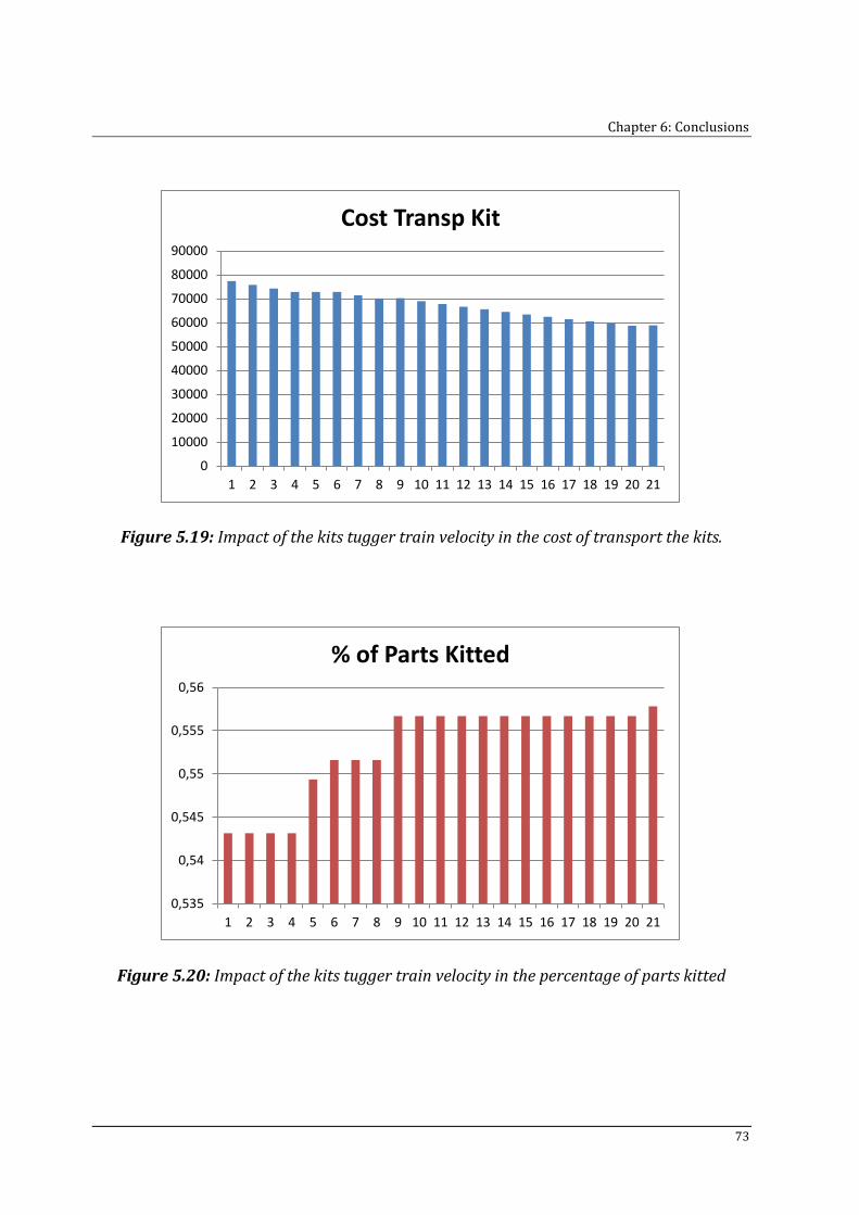
Chapter 6: Conclusions
73
Figure 5.19: Impact of the kits tugger train velocity in the cost of transport the kits.
Figure 5.20: Impact of the kits tugger train velocity in the percentage of parts kitted
0
10000
20000
30000
40000
50000
60000
70000
80000
90000
1 2 3 4 5 6 7 8 9 10 11 12 13 14 15 16 17 18 19 20 21
Cost Transp Kit
0,535
0,54
0,545
0,55
0,555
0,56
1 2 3 4 5 6 7 8 9 10 11 12 13 14 15 16 17 18 19 20 21
% of Parts Kitted
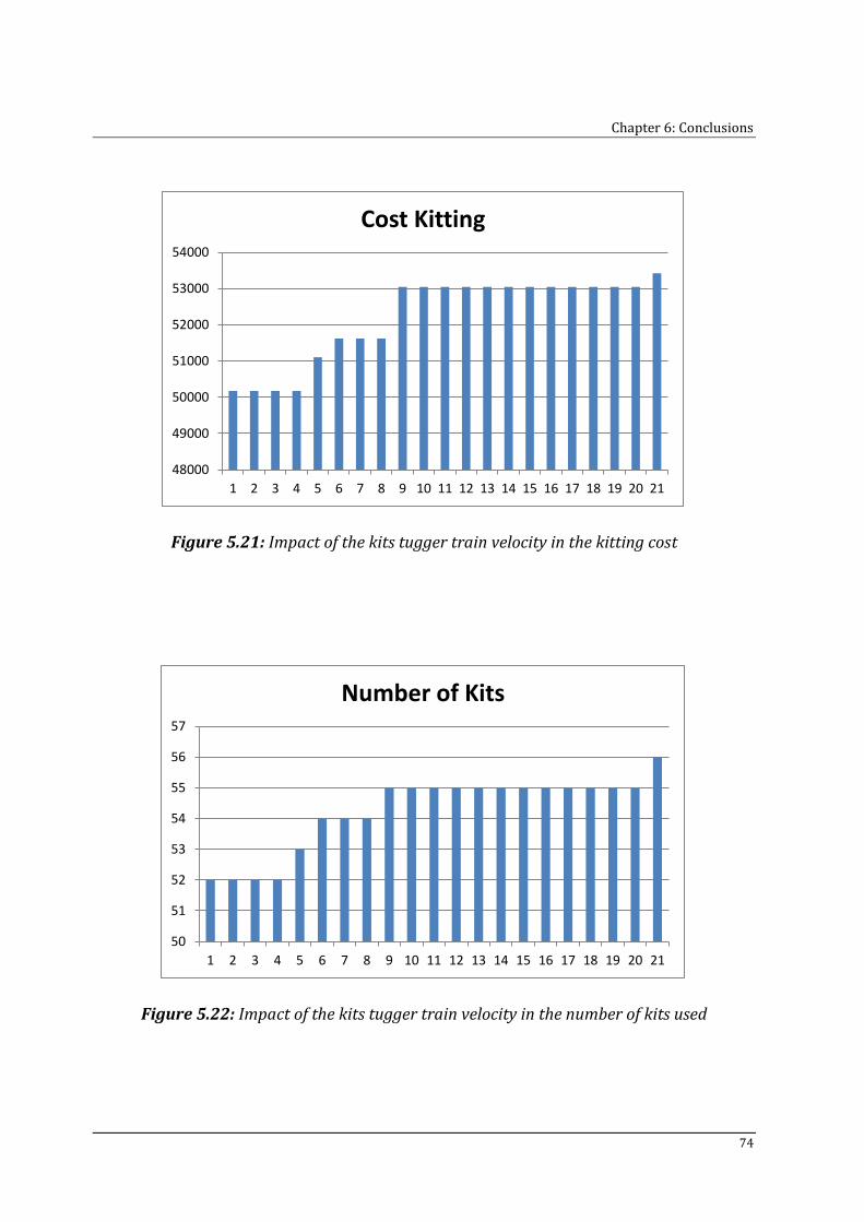
Chapter 6: Conclusions
74
Figure 5.21: Impact of the kits tugger train velocity in the kitting cost
Figure 5.22: Impact of the kits tugger train velocity in the number of kits used
48000
49000
50000
51000
52000
53000
54000
1 2 3 4 5 6 7 8 9 10 11 12 13 14 15 16 17 18 19 20 21
Cost Kitting
50
51
52
53
54
55
56
57
1 2 3 4 5 6 7 8 9 10 11 12 13 14 15 16 17 18 19 20 21
Number of Kits
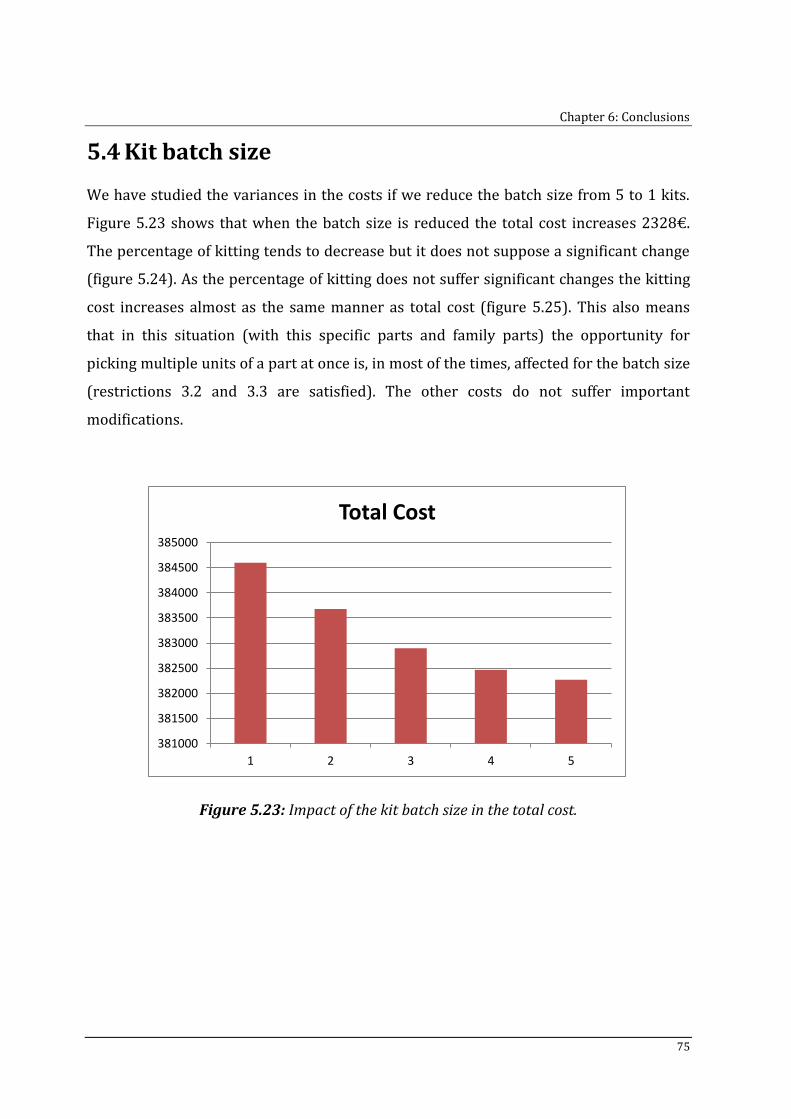
Chapter 6: Conclusions
75
5.4 Kit batch size
We have studied the variances in the costs if we reduce the batch size from 5 to 1 kits.
Figure 5.23 shows that when the batch size is reduced the total cost increases 2328€.
The percentage of kitting tends to decrease but it does not suppose a significant change
(figure 5.24). As the percentage of kitting does not suffer significant changes the kitting
cost increases almost as the same manner as total cost (figure 5.25). This also means
that in this situation (with this specific parts and family parts) the opportunity for
picking multiple units of a part at once is, in most of the times, affected for the batch size
(restrictions 3.2 and 3.3 are satisfied). The other costs do not suffer important
modifications.
Figure 5.23: Impact of the kit batch size in the total cost.
381000
381500
382000
382500
383000
383500
384000
384500
385000
1 2 3 4 5
Total Cost
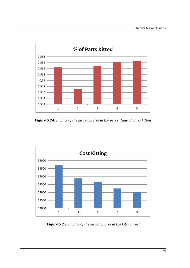
Chapter 6: Conclusions
76
Figure 5.24: Impact of the kit batch size in the percentage of parts kitted.
Figure 5.25: Impact of the kit batch size in the kitting cost
0,542
0,544
0,546
0,548
0,55
0,552
0,554
0,556
0,558
1 2 3 4 5
% of Parts Kitted
52000
52500
53000
53500
54000
54500
55000
1 2 3 4 5
Cost Kitting
Chapter 6: Conclusions
77
5.5 Available space at the border of the line
As mentioned in chapter 3, we will study how the cost varies is if we vary the available
length at the border of the line. Not all the space available is always used and we want to
study how important it could be in the total cost to use more space.
To study it we have obtained the results when the length factor varies from 1 to 2 in
steps of 0.125. As the standard size is 8 meters (Ph.D. of dr. Veronique Limère), it means
that we are obtaining the results in steps of 1 meter from 8 to 16 meters.
As this change permits a bigger slack to the restriction (2.13), the total cost will always
decrease. However, we can see in Figure 5.26 that, as the space available value becomes
bigger, the impact in the cost is smaller.
For this reason we have reduced the interval from 8 to 12 meters giving the results
obtained every half meter. As it happens the same that in the first study (the impact in
the cost is much more significant in the first meters), we have reduced again the interval
from 8 to 10 giving the results every 0.25 meters (which corresponds with a lower value
of 1 in the length factor, an upper value of 1.25 and a step value of 0.03125). We can see
in figure 5.27 that if the available space at the border of the line is extended in 2 meters
(from 8 meters to 10), we obtain a save of 11143€, which suppose a 2.9% of the total
cost. Moreover, only extending half a meter the length (until 8.5 meters) we will also
have an important save (5220€, that corresponds to a 1.36% of the total cost). The
percentage of parts kitted tends to decrease (figure 5.28) as more space is available and
more bulks can be allocated at the border of the line. As it, the number of kits used also
decreases (figure 5.29).
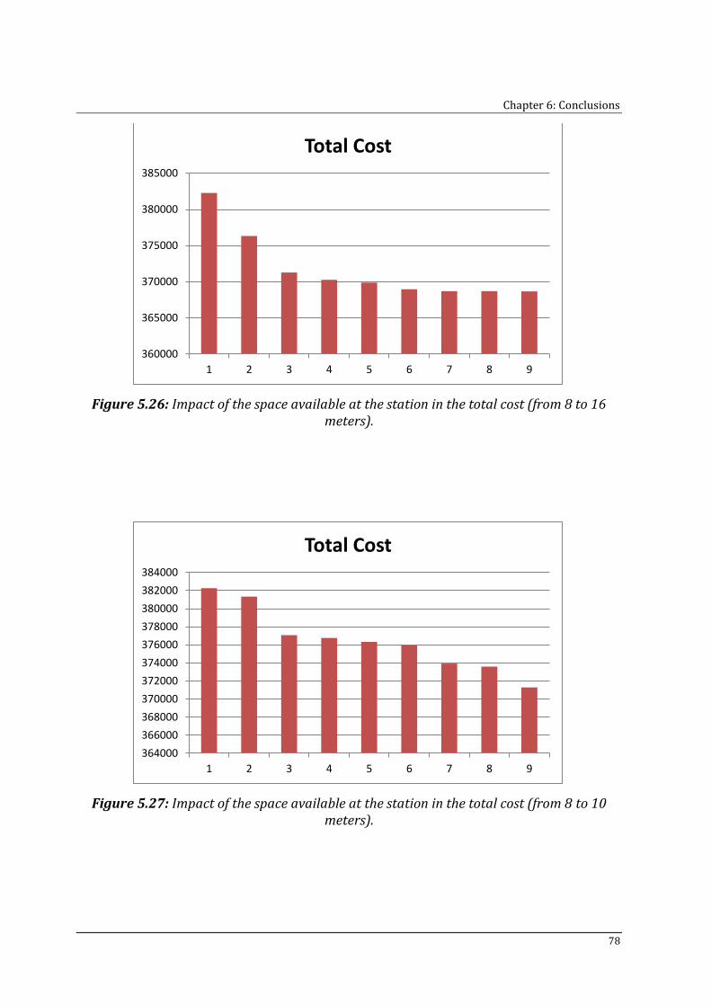
Chapter 6: Conclusions
78
Figure 5.26: Impact of the space available at the station in the total cost (from 8 to 16 meters).
Figure 5.27: Impact of the space available at the station in the total cost (from 8 to 10 meters).
360000
365000
370000
375000
380000
385000
1 2 3 4 5 6 7 8 9
Total Cost
364000
366000
368000
370000
372000
374000
376000
378000
380000
382000
384000
1 2 3 4 5 6 7 8 9
Total Cost
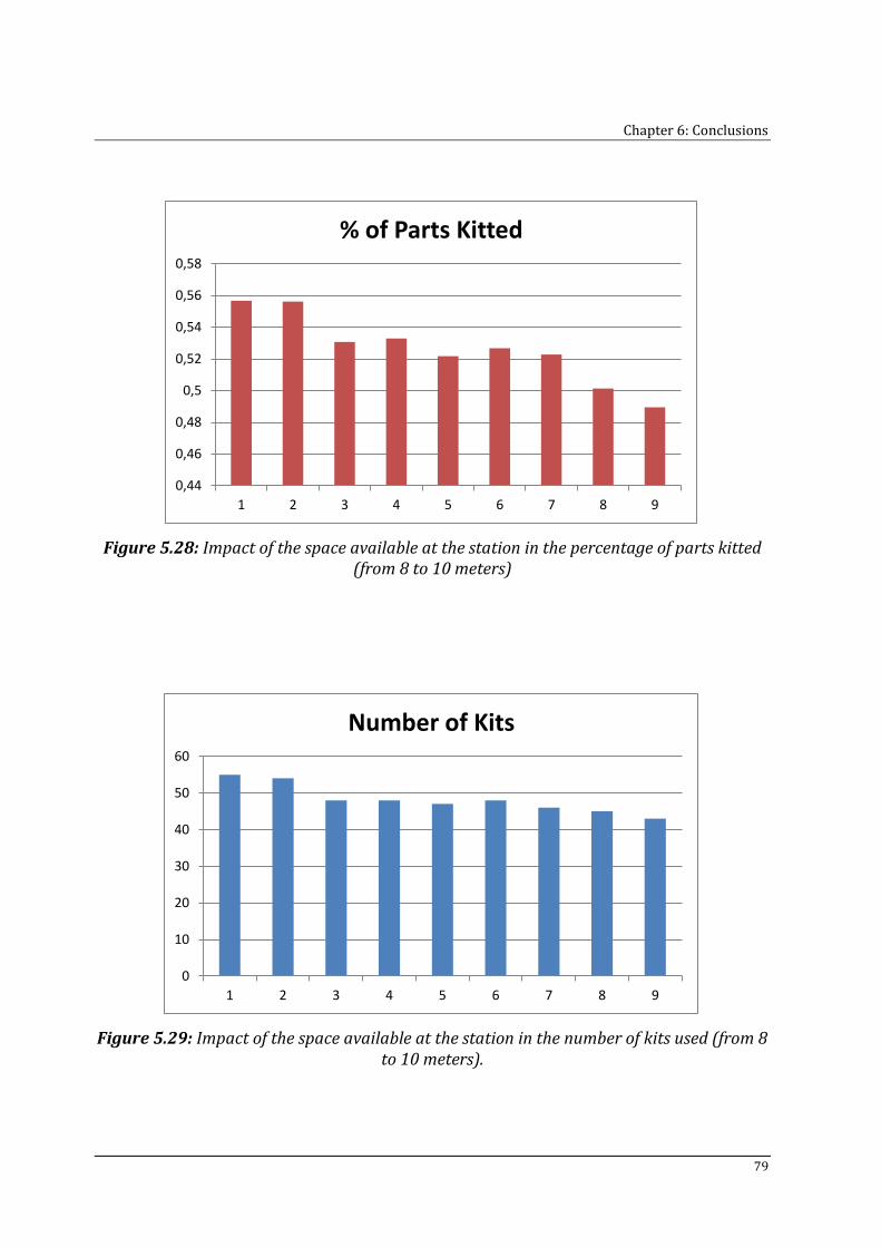
Chapter 6: Conclusions
79
Figure 5.28: Impact of the space available at the station in the percentage of parts kitted (from 8 to 10 meters)
Figure 5.29: Impact of the space available at the station in the number of kits used (from 8 to 10 meters).
0,44
0,46
0,48
0,5
0,52
0,54
0,56
0,58
1 2 3 4 5 6 7 8 9
% of Parts Kitted
0
10
20
30
40
50
60
1 2 3 4 5 6 7 8 9
Number of Kits
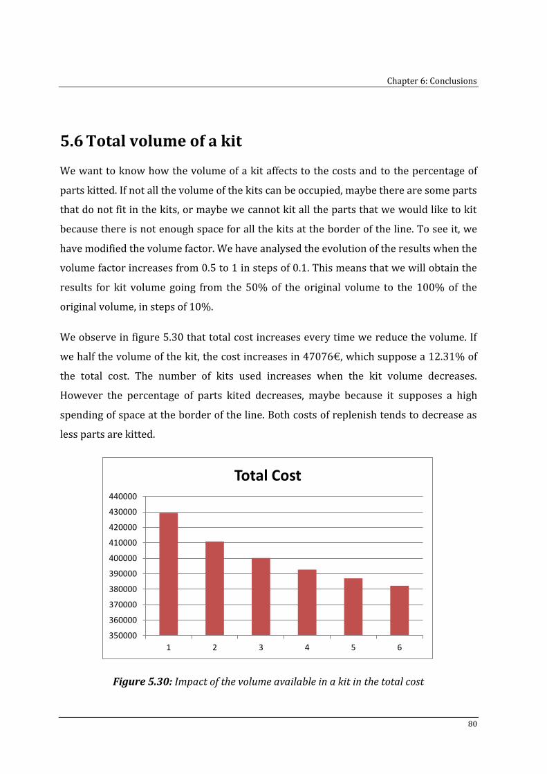
Chapter 6: Conclusions
80
5.6 Total volume of a kit
We want to know how the volume of a kit affects to the costs and to the percentage of
parts kitted. If not all the volume of the kits can be occupied, maybe there are some parts
that do not fit in the kits, or maybe we cannot kit all the parts that we would like to kit
because there is not enough space for all the kits at the border of the line. To see it, we
have modified the volume factor. We have analysed the evolution of the results when the
volume factor increases from 0.5 to 1 in steps of 0.1. This means that we will obtain the
results for kit volume going from the 50% of the original volume to the 100% of the
original volume, in steps of 10%.
We observe in figure 5.30 that total cost increases every time we reduce the volume. If
we half the volume of the kit, the cost increases in 47076€, which suppose a 12.31% of
the total cost. The number of kits used increases when the kit volume decreases.
However the percentage of parts kited decreases, maybe because it supposes a high
spending of space at the border of the line. Both costs of replenish tends to decrease as
less parts are kitted.
Figure 5.30: Impact of the volume available in a kit in the total cost
350000
360000
370000
380000
390000
400000
410000
420000
430000
440000
1 2 3 4 5 6
Total Cost
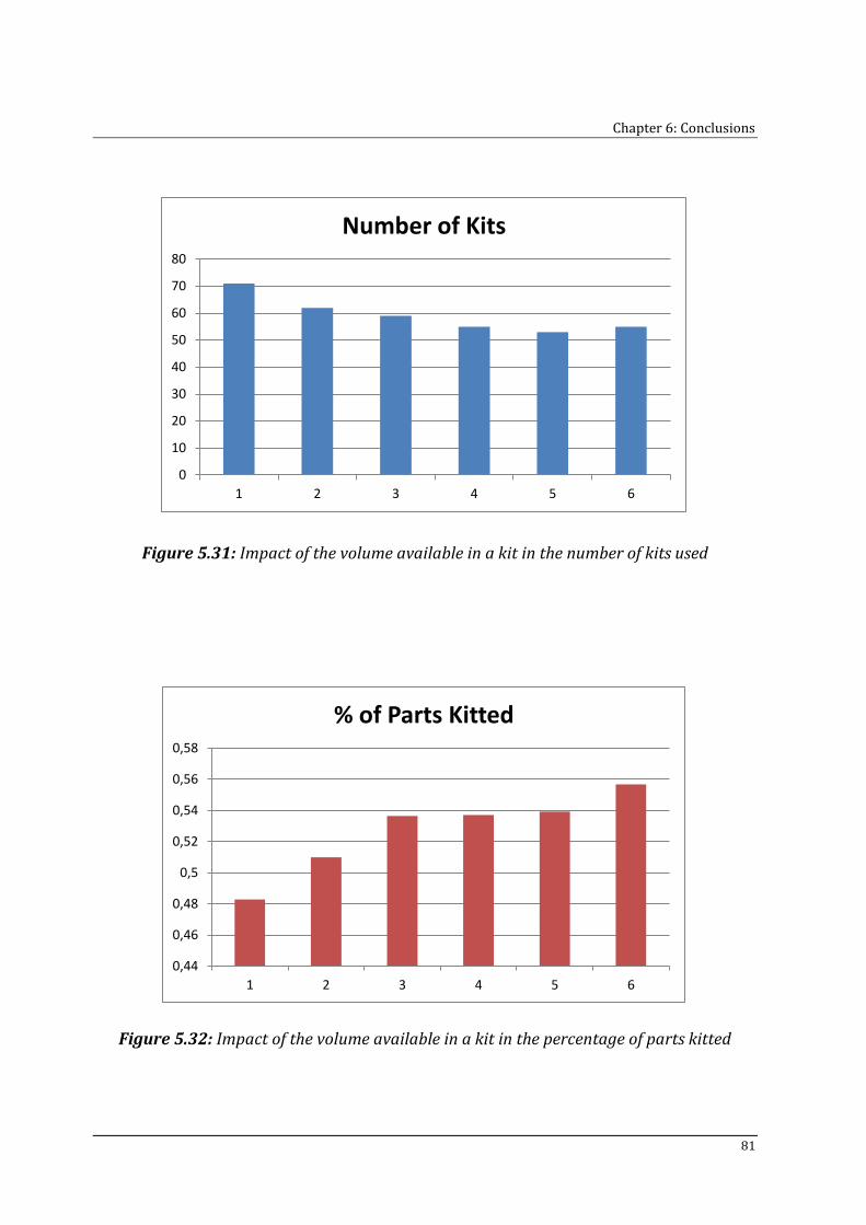
Chapter 6: Conclusions
81
Figure 5.31: Impact of the volume available in a kit in the number of kits used
Figure 5.32: Impact of the volume available in a kit in the percentage of parts kitted
0
10
20
30
40
50
60
70
80
1 2 3 4 5 6
Number of Kits
0,44
0,46
0,48
0,5
0,52
0,54
0,56
0,58
1 2 3 4 5 6
% of Parts Kitted
Chapter 6: Conclusions
82
Chapter 6 Conclusions
This thesis is a further research of the Ph.D. realized by Veronique Limère: “To Kit or Not
to Kit: Optimizing Part Feeding in the Automotive Assembly industry”.
On the one hand, this thesis deals with the development of a tool in order to facilitate
and make more comfortable the work for the employees of a company using it. The
work tool is created to complement the mathematical model realized in the Ph.D.
mentioned before. For this reason it can only be used in factories where the
mathematical model is implemented. This model supports the best choice between two
supply systems: bulk feeding and kitting.
On the other hand, in this thesis we have considered the possibility that factories can
suffer some modifications in the way they supply the materials. We have used the tool to
analyse the differences that these modifications can lead.
Answering to the first point, the tool developed satisfies all the requisites needed:
First of all we have to mention the fact that it has been developed in an excel file. Excel is
one of the most used programs in companies. Therefore it the makes work of the
Chapter 6: Conclusions
83
employee more comfortable. Moreover the fact that the employee using the tool only has
to fill a template to obtain the results makes it even more comfortable.
Secondly, as it has been required, it allows us to study how the costs and the number of
parts kitted varies when one or more parameters also varies between two values (lower
value and upper value) with an interval between two consecutives values (step value). It
let us now the tendency that results follows.
Finally, it gives us the results in a sheet and also in graphs, which helps the employee to
analyse the results. Moreover, it informs about the feasibility of the solution.
In order to answer the second point, we have used the tool to realize a study with the
data of a particular company. If all the others parameters keep the original value, we
have concluded that:
If we are using a new picking technology in the supermarket, for every 0.1 seconds that
the searching time is reduced, we have a saving of 0.24% of the total cost, and the
percentage of parts kitted tends to increase while we reduce the searching time.
The reduction of the labour cost for kitting operations if the company is outsourcing
(from 30€ to 20€), reduces de total cost in a 4.6%. Moreover, if the distance between the
factory and the 3PL increases, the total cost tends to increase, and the percentage of
parts kitted tends to decrease.
Increasing the forklift velocity diminishes the total cost in 15.312€ and it is directly
proportional to the velocity, as the time that the operator spends on transporting the
pallets is lower. However, it does not have a significant repercussion in the number of
parts kitted. The same happens if we increase the velocity of the tugger train
transporting kits.
Reducing the batch size from 5 kits to 1 kit does not lead to a significant change in the
percentage of parts kitted. Moreover, the reduction of the total cost only changes in
2328€.
Chapter 6: Conclusions
84
Increasing the available length along the workstation reduces the total cost, as it is a
restrictive factor. However, for every half meter it increases, the reduction that the total
cost suffers is less. Increasing the length available from 8 to 8.5 will suppose a reduction
of a 1.26% of the total cost. On the other hand, the percentage of parts kitted, tends to
decrease in a considerable value if the space available increases.
The total cost increases every time the kit volume is reduced. If we half the volume of
the kit, the total cost increases in a 12,31%. The percentage of parts kitted diminishes in
a significant way (from55.66% to 48.27%).
References
Boysen, N., Bock, S., 2011. Scheduling just-in-time part supply for mixed-model assembly lines. European Journal of Operational Research 211 (1), 15–25.
Bozer, Y. A., Mcginnis, L. F., 1992. Kitting versus line stocking - a conceptual-framework and a descriptive model. International Journal of Production Economics 28 (1), 1–19.
Choobineh, F., Mohebbi, E., 2004. Material planning for production kits under uncertainty. Production Planning & Control 15 (1), 63–70.
Ding, F., Puvitharan, B., 1990. Kitting in just-in-time production. Production and Inventory Management Journal 31 (4), 25–28.
Ding, F. Y., 1992. Kitting in jit production: a kitting project at a tractor plant.
Industrial Engineering.
Limère, V., 2011. To Kit or Not to Kit: Optimizing Part Feeding in the automotive
assembly Industry. Universiteit Gent.
Limère, V., Van Landeghem, H., Goetschalckx, M., Aghezzaf, E-H., Mc Ginnis, L., 2011.
Optimizing materials feeding in the automotive industry: kitting and line stocking.
International Journal of Production Research. DOI:10.1080/00207543.2011.588625.
Swaminathan, J., Nitsch, T., 2007. Managing product variety in automobile assembly:
The importance of the sequencing point. Inter- faces 37 (4), 324–333.
Chapter 6: Conclusions
86
Wanstrom, C., Medbo, L., 2009. The impact of materials feeding de- sign on assembly
process performance. Journal of Manufacturing Technology Management 20 (1), 30-
51.
Web sites:
http://www.grupov10.com/pickbyvoice.html
http://www.dematic.com/com/Productos/Tecnologas-de-Picking/Pick-by-Light/page35605.htm
http://pymecrunch.com/pick-to-vision-picking-por-guiado-optico
http://www.ampl.com/
https://groups.google.com/group/ampl?pli=1
http://www.todoexcel.com/foro-excel/tus-preguntas/