Anke Schaffartzik • Magdalena Sachs •

Dominik Wiedenhofer • Nina Eisenmenger

Environmentally Extended Input-Output Analysis

S O C I A L E C O L O G Y W O R K I N G P A P E R 1 5 4

September 2014ISSN 1726-3816

Anke Schaffartzik, Magdalena Sachs, Dominik Wiedenhofer, Nina Eisenmenger (2014):

Environmentally Extended Input-Output Analysis

Social Ecology Working Paper 154 Vienna, September 2014

ISSN 1726-3816

Institute of Social Ecology IFF - Faculty for Interdisciplinary Studies (Klagenfurt, Graz, Vienna) Alpen-Adria-Universitaet Schottenfeldgasse 29 A-1070 Vienna

www.aau.at/socec workingpaper@aau.at

© 2014 by IFF – Social Ecology

Environmentally Extended Input-Output Analysis

Authors: Anke Schaffartzik Magdalena Sachs Dominik Wiedenhofer Nina Eisenmenger

Table of Contents

1. Introduction ............................................................................................................................ 1

2. The Basics of Input-Output Analysis ..................................................................................... 2

2.1 Introduction to Input-Output Tables .............................................................................................. 2

2.2 Input-Output Analysis and the Leontief Inverse ........................................................................... 4

3. Environmentally Extended Input-Output Analysis (EEIOA) ................................................ 8

3.1 Leontief’s Example ....................................................................................................................... 8

3.2 EEIOA Example for a Hypothetical Economy ........................................................................... 11

4. Call for Caution .................................................................................................................... 14

5. References ............................................................................................................................ 17

Figures and Tables

Table 1: Simplified Input-Output Table for a Hypothetical Three-Product ............................... 3

Table 2: Overview of Typical Element Notation within an Input-Output Table ....................... 3

Table 3: Matrix A of Technical Coefficients for a Hypothetical Three-Product Economy ....... 6

Info-Box: Power Series Approximation ..................................................................................... 7

Table 4: Leontief Inverse for a Hypothetical Three-Product Economy ..................................... 8

Figure 1: Environmental extension of the IO framework based on the physical input-output table (PIOT) as originally presented by Leontief ..................................................................... 10

Figure 2: PIOT, MIOT, and Leontief inverses for six-activity hypothetical economy ............ 12

Figure 3: Material requirements associated with domestic and exported final demand (yd and yex) in the hypothetical economy ............................................................................................ 13

1

1. Introduction

Social ecology research centers on the understanding that in order to contribute to meaningful analysis of current sustainability challenges, it is necessary to consider both sociocultural and biophysical interrelations (Fischer-Kowalski and Weisz, 1999). It may seem self-evident that economies indispensably require energy and material inputs as well as the discharge of wastes in order to function. Yet, a dominant paradigm maintains that boundless economic growth is possible. Such an approach to development does not take into account the biophysical limitations of society’s metabolism and thus ignores given “limits to growth” (Ayres and Kneese, 1969; Daly, 1973; Meadows et al., 1972). Nonetheless, important advances have been made in considering human societies not only in terms of their economic but also their biophysical dimensions in acknowledging that societies do have a “metabolism” (Fischer-Kowalski and Haberl, 1998). Alongside the concept of social metabolism, a corresponding tool was developed which, instead of regarding an economy purely in monetary terms, accounts for society’s biophysical inputs and outputs. Economy-wide material flow accounts document material use in mass units, most commonly metric tons. The considered material flows include all materials an economy extracts from its domestic environment, imports from other and exports to other economies as well as discharges to the environment (Fischer‐Kowalski et al., 2011; Weisz et al., 2007). From its beginnings in academia, this approach continuously gained wider acceptance together with the notion that growth in a physically finite world must be limited. Indicators derived from material flow accounts have become an integral part of environmental accounting (European Commission, 2011).

As the underlying methodology matured, so did the interest in applying it to new research questions. As we potentially face planetary boundaries (Rockström et al., 2009), these increasingly relate to understanding what drives (and has the potential to curb) our global resource use. The latter requires a more in-depth understanding of the structures and dynamics of resource use than can be gained from material flow accounts. The ‘black box’ as which MFA treats society must be opened. In this Working Paper, we will examine the application of economic input-output modelling in social ecology as a means to open up this black box. Input-output models are used in economics to represent the structure of production and final consumption within an economy (single-region input-output SRIO model) or amongst multiple economies (multi-region input-output MRIO model). These models depict by economic activity (e.g. agriculture, food production, restaurant services) the inputs required from other economic activities (e.g. food production would buy inputs from agriculture and restaurant services would buy inputs from food production) and the output provided either to other activities or to final consumption (including public as well as private spending as well as exports). Although this type of structure could also be depicted in physical units of mass or energy, data is typically only collected in monetary units (see Weisz and Duchin, 2006) and serves as the basis for calculating the gross domestic product (GDP) as the market value of all goods and services produced within an economy during a specific year. Input-output data can be used to trace the impact of changes in final consumption on production structures. Such an application also allows for the calculation of the inputs required to produce goods and services for export.

Input-output analysis can be “environmentally extended” (environmentally extended input-output analysis (EEIOA)) by integrating information from physical accounting, for example, on energy or material use or pollution, into the input-output model. Because the input-output model is in monetary units and the environmental extension is in physical units (e.g. in joules of energy, tons of material, or kilograms of pollutant), this integration is non-trivial. A number of assumptions have to be made, the validity of which has a significant impact on how we can

2

interpret the results (see section 4). EEIOA is increasingly being used as a tool to understand the material or energy requirements or the environmental burden associated with specific sectors or with the components of final demand, e.g., for domestic final demand and exports. Where the input-output table is extended by material flows, material inputs are allocated to production sectors and can then be linked to the final demand which they ultimately satisfy. With regard to exports, EEIOA allows for an approximation of the upstream material requirements of the production of traded goods. Resource extraction, not matter where in the world it occurs, is linked to the final demand for goods and services in the country under investigation. This type of consumption-based approach to material flow accounting complements the production-based approach (oriented towards the material use in national economies).

In order to be able to interpret these types of accounts, it is important that the social ecologist have a working knowledge of the fundamentals of environmentally extended input-output analysis and be familiar with applications and limitations of the method. In this Working Paper, we will provide an introduction to input-output analysis and its environmental extension including step-by-step calculations based on the model of a hypothetical economy. We follow up with a discussion of the assumptions which go into this type of approach. The aim of this Working Paper is to make the important EEIOA tool accessible to students and researchers of social ecology.

2. The Basics of Input-Output Analysis

In the following section, we will provide a very basic introduction to the general structure of and calculations behind environmentally extended input-output analysis. Readers wishing to study the method in greater detail and variation will find a wealth of useful information in the standard textbook by Miller and Blair (2009) and the manual provided by Eurostat (2008). We will begin with an introduction to the structure and elements of input-output tables and then move on to the logic and the calculations behind their environmental extension.

2.1 Introduction to Input-Output Tables

Input-output tables (IOTs) depict the structure of an economy and include both the inter-industry relations in its productive and service sectors and the composition of final demand. The inputs required by each economic activity (or sector) to produce that activity’s output to both other activities and to final demand are recorded. Although it is possible to construct IOTs in physical units (tons, for example), sufficiently robust data for such tables is hardly available in practice (see Weisz and Duchin, 2006). In monetary units, IOTs are compiled routinely by the national statistical offices1 and, since they record the value of all goods and services produced for final consumption in an economy within a given year, serve as the basis for calculating the gross domestic product (GDP).

1 For example, the Austrian supply, use, and input-output tables are available here: http://www.statistik.at/web_en/statistics/national_accounts/input_output_statistics/index.html. Eurostat publishes the input-output tables of all EU member states here: http://epp.eurostat.ec.europa.eu/portal/page/portal/esa95_supply_use_input_tables/data/workbooks.

3

Table 1: Simplified Input-Output Table for a Hypothetical Three-Product

Table 1 depicts a simplified IOT of a hypothetical economy which only produces three goods (and these goods are produced by three corresponding economic activities): wood, paper, and books. The values in the columns show which inputs are required for the production of all the wood, paper, and books in this economy. For example, 90 units worth of wood, 10 of paper, and 5 of books are needed to produce the total amount of paper. While the top left 3x3 section of the table depicts the inter-industry flows, the fourth column shows the final demand. Final demand is shown as an aggregate value in this example. In ‘real-life’ input-output tables, domestic and foreign final demand (exports) are typically differentiated. Domestic final demand usually consists of the final demand of households and government and NGOs. Changes in inventories and capital formation (gross fixed capital formation GFCF) are also commonly reported as categories of final demand. For the latter category the argument might be made that capital formation corresponds to inputs into (future) production. The total output of each of the products corresponds to the sum of inter-industry use and final demand and is represented in the column on the very right. In monetary terms, value is added to a product during the production process. This happens because labor, taxes, interest, rent, and profit have to be paid for. The value added is shown in the fourth row. Only as many units of a product can be consumed within the economy as are generated. Therefore, the totals by column and by row have to match.

Table 2: Overview of Typical Element Notation within an Input-Output Table

matrix Z with elements zij: interindustry flows

vector y with elements yi: final demand

vector x with elements xi: total output

vector v with elements vi: value added

vector x’ with elements xi: total outlays

In order to facilitate our communication about input-output tables, we can use typical matrix notation. The input-output table can be divided into several sections or matrices and vectors: The interindustry relations, i.e. the 3x3 matrix with wood, paper, and books heading the columns and the rows in Table 1, is often denoted by the capital letter Z. Its elements can accordingly be represented by z11, z12, …, zij where the first index (i) represents the row number and the second index (j) represents the column number corresponding to the element (see Table

Wood Paper Books Final Demand Total Output

Wood 85 90 0 20 195

Paper 10 10 90 200 310

Books 5 5 20 500 530

Value Added 95 205 420 720

Total 195 310 530 720 1755

1 2 … j y x

1 z11 z12 … z1j y1 x1

2 z21 z22 … z2j y2 x2

… … … … … … …

i zi1 zi2 … zij yi xi

v v1 v2 … vi

x' x1 x2 … xi Y X

4

2). In Table 1, for example, the flow of books into paper production would be represented by element z32. The input-output table also contains a vector y of final demand (represented by a single vector in Table 1 and 2 but often disaggregated by household and government consumption as well as exports in ‘real’ IOTs). Vector x contains the total output (whether for interindustry use or final demand) by each economic activity. Transposed into a row vector (x’), it is usually referred to as total outlays. The elements in both vectors are identical because total outlays must equal total output for each activity or product. The vector v represents the value added.

Within the input-output table, total inputs equal total outputs: This is the mass balance principle in economic terms. In simplified terms, the economic value of the all the flows into one activity equal the value of all of the flows from that activity to other activities or final demand, for example:

z11 + z12 + … + z1j + y1 = z11 + z21 + … +zi1 +v1 = x1 (Table 2)and 85 + 90 + 0 + 20 = 85 + 10 + 5 + 95 = 195 (Table 1)

For the sake of simplicity, all of the following calculations refer to square (n x n) matrices, i.e. to matrices with the same number of rows and columns (n). Input-output tables may, however, be asymmetrical (i.e., non-square) and depict more than one type of output from each industry, for example.

2.2 Input-Output Analysis and the Leontief Inverse

The term “input-output analysis” is often used to indicate that input-output structures are being investigated on the basis of input-output tables. We will deal here with only one very central aspect of this analysis which will be decisive for our environmental extensions: The Leontief inverse. This calculation is named in honor of the Russian economist Wassily Leontief who laid the methodological groundwork on which present-day EEIOA is based (Leontief, 1970, 1986).

Before we delve into the calculations: Why do we even need to calculate anything further? The input-output table for our hypothetical economy (Table 1) informs us on how much wood, paper, and books were needed to produce the 20 units worth of wood, 200 units of paper, and 500 units of books required by final demand. Often, however, we will be interested in understanding the intermediate inputs associated with one unit of final demand rather than with the total final demand. We might ask questions like: How much wood must be bought in order to produce one unit of books for final demand? How much wood could be ‘saved’ if we reduced final demand by one unit? If final demand for books increases by one unit, what would be the effect on the wood and paper producing activities? We cannot answer these questions directly based on Table 1 but a few simple mathematical equivalence operations will get us there.

The first transformation we will perform yields the matrix of direct intermediate input requirements (also called technical coefficients) which is denoted by the capital letter A. Each element in aij in A will represent the amount of inter-industry inputs directly required to produce one unit of output. The calculation in itself is very simply: Each element of the matrix of interindustry flows Z is divided by the total output (x) of that activity to which it contributes. In matrix notation this calculation reads:

5

= × (F1)

In order to divide each element of Z by the corresponding total output, we multiply Z with diagonalized (indicated by the hat symbol) inverse (indicated by -1) of x. Multiplying with the inverse is equivalent to dividing and the diagonalization (into an nxn matrix with the values of x-1 along the diagonal) allows us to use matrix multiplication. For our example (Table 1) both

the inverse of x (x-1) and the diagonalization of that inverse () are shown below:

=0.0050.0030.002

(F2)

=0.005 0 00 0.003 00 0 0.002

(F3)

By multiplying the matrix Z of interindustry flows (from Table 1) with the diagonalized inverse of total production (F3), we obtain the matrix of technical coefficients A:

=85 90 010 10 905 5 20

×0.005 0 00 0.003 00 0 0.002

=. . . . . . . .

(F4)

Please note that the vector in F2 and the matrix F3 have been rounded to the third decimal place. Therefore, the calculation in F4 will render a slightly different result if the rounded values are copied; the result presented in F4 stems from matrix multiplication using spreadsheet software and is not based on rounded values. The value “0” (with no decimal places reported) represents a true (and not a rounded) zero. Since all we have done is transform matrix Z, we can also easily ‘reverse’ our calculations: If we have calculated A correctly, then multiplying it with the diagonalized vector of total output ( ) will yield matrix Z.

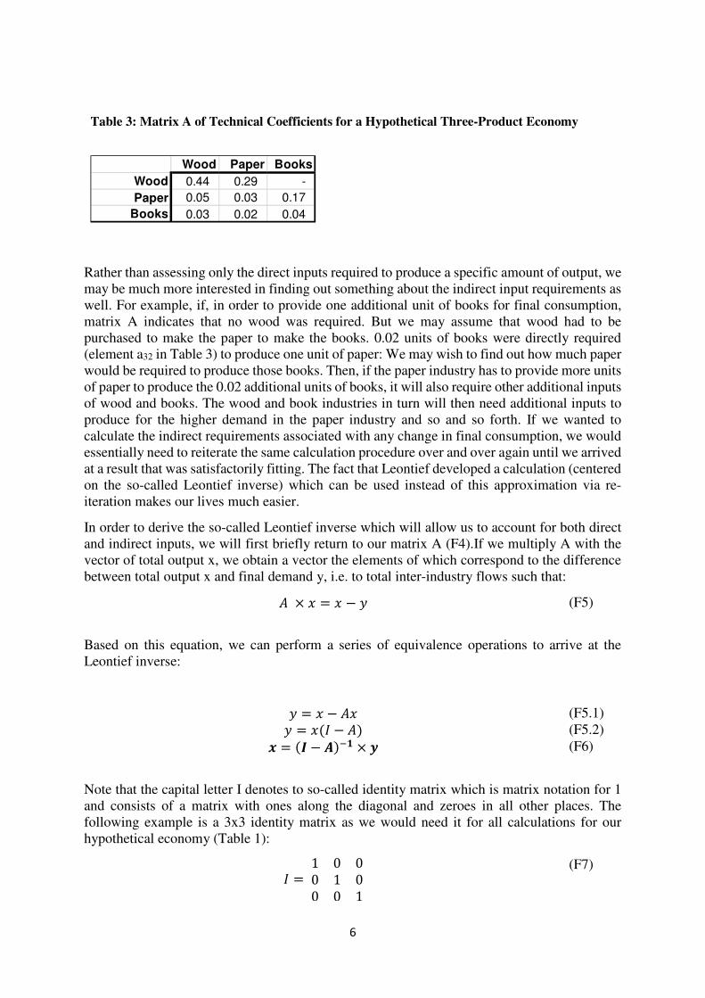
This matrix A of technical coefficients allows us to easily assess the amount of inter-industry inputs required to produce one unit’s worth of output to final demand. For example, in order to supply one unit of paper to final demand, 0.29 units of wood were directly required (element a12 in Table 3). Please note that in spreadsheet software the symbol “-” (a13 in Table 3) is sometimes used to represent a ‘true’ (as opposed to a rounded) zero. If the value in a13 in this case were “0.00”, this would mean that the cell contains a value larger than zero rounded to the nearest hundredth.

6

Table 3: Matrix A of Technical Coefficients for a Hypothetical Three-Product Economy

Rather than assessing only the direct inputs required to produce a specific amount of output, we may be much more interested in finding out something about the indirect input requirements as well. For example, if, in order to provide one additional unit of books for final consumption, matrix A indicates that no wood was required. But we may assume that wood had to be purchased to make the paper to make the books. 0.02 units of books were directly required (element a32 in Table 3) to produce one unit of paper: We may wish to find out how much paper would be required to produce those books. Then, if the paper industry has to provide more units of paper to produce the 0.02 additional units of books, it will also require other additional inputs of wood and books. The wood and book industries in turn will then need additional inputs to produce for the higher demand in the paper industry and so and so forth. If we wanted to calculate the indirect requirements associated with any change in final consumption, we would essentially need to reiterate the same calculation procedure over and over again until we arrived at a result that was satisfactorily fitting. The fact that Leontief developed a calculation (centered on the so-called Leontief inverse) which can be used instead of this approximation via re-iteration makes our lives much easier.

In order to derive the so-called Leontief inverse which will allow us to account for both direct and indirect inputs, we will first briefly return to our matrix A (F4).If we multiply A with the vector of total output x, we obtain a vector the elements of which correspond to the difference between total output x and final demand y, i.e. to total inter-industry flows such that:

× = − (F5)

Based on this equation, we can perform a series of equivalence operations to arrive at the Leontief inverse:

= − (F5.1) = ( − ) (F5.2)

= ( − ) × (F6)

Note that the capital letter I denotes to so-called identity matrix which is matrix notation for 1 and consists of a matrix with ones along the diagonal and zeroes in all other places. The following example is a 3x3 identity matrix as we would need it for all calculations for our hypothetical economy (Table 1):

=1 0 00 1 00 0 1

(F7)

Wood Paper Books

Wood 0.44 0.29 -

Paper 0.05 0.03 0.17

Books 0.03 0.02 0.04

7

The elements in the Leontief inverse ( − ) reflect both the inputs required directly and indirectly to produce one (additional) unit of final demand. The matrix in parentheses is taken to the power of negative 1: This is the inverse of the matrix. The inverse of a matrix C is defined such that × = where I is the identify matrix (see F7). Not all matrices are invertible: A matrix for which the determinant (det(C)) is equal to 0 is a singular, non-invertible matrix. The determinant of a matrix

=

is calculated as det() = ( + +) − ( + +) .

Info-Box: Power Series Approximation

How the simple-looking equation ( − ) can reflect both the inputs required directly and indirectly to produce one (additional) unit of final becomes clearer when we consider how we would calculate the approximation of direct and indirect inputs in a re-iterative procedure. Such a procedure exists because the inversion of large matrices requires quite some computational power which was not always available: Miller and Blair (2009) report that in 1939, it took 52 hours to invert a 42x42 matrix and even in 1970, Leontief warned his readers that computing the inverse for larger matrices would require a computer, indicating that he did not use one for the examples with which he illustrated his approach (Leontief, 1970). The procedure by which the Leontief inverse can be approximated without requiring the calculation of an actual inverse is known as the power series approximation. If we take a power series L such that

= + + + + ⋯+ (F8)

and we multiply this series by A, we obtain × = + + + ⋯+ (F9)

For elements of the technical coefficient matrix aij for all of which 1 > |a| holds true, as n approaches infinity, the an value approaches 0. Therefore, − × = and × ( − ) = . If we multiply both sides of the latter equation with ( − ), we obtain = ( − ) × . Since I is the identity matrix and multiplication with I corresponds to multiplication with 1 in matrix terms, this can simply be expressed as = ( − ). The power series is a fairly good approximation of the Leontief inverse and giving us some sense of the calculation process that would be necessary if we didn’t have the tool of the Leontief inverse and the necessary computational power at our disposal. In our hypothetical economy of wood, paper, and books, we left off with the A matrix of technical coefficients (Table 3) and are now ready to apply Leontief’s calculation to it. In order to calculate (I-A), we need a 3x3 identity matrix (F7):

( − ) =1 0 00 1 00 0 1

−0.44 0.29 00.05 0.03 0.170.03 0.02 0.04

=0.56 −0.29 0−0.05 0.97 −0.17−0.03 −0.02 0.96

(F10)

When we invert this matrix (I-A) we obtain the Leontief inverse the elements of which inform us about the direct and indirect inputs required so that one (additional) unit of final demand can be met.

Including indirect input requirements changes the matrix quite a bit as compared to the matrix technical coefficients. We can now see, for example, that while no purchases of wood were made directly to satisfy final demand for books, 0.1 units of wood were required as an indirect input (Table 4).

8

Table 4: Leontief Inverse for a Hypothetical Three-Product Economy

Keeping mind our equation F6, we know that multiplying the Leontief inverse with final demand y should yield total output x:

=1.83 0.55 0.100.11 1.07 0.190.05 0.03 1.04

×20200500

=195310530

(F11)

In a more detailed input-output model in which final demand is disaggregated by different categories (household and government spending and exports), we could substitute any of these vectors for the vector y of total final demand in F11 and thus calculate the input requirements associated only with household spending or with exports.

3. Environmentally Extended Input-Output Analysis (EEIOA)

Until now, we have been dealing with abstract monetary ‘units’ of spending in our input-output tables. In this section, we will explore how environmental extensions introduce physical units into the input-output model. In doing so, we will initially reconstruct the example that Leontief used to set forth his approach which was based on a physical rather than a monetary input-output table. We will then offer insights from another hypothetical economy (this one based on biomass rather than books) in the following section.

3.1 Leontief’s Example

In 1970, economist Wassily Leontief published an article in which he proposed using what is now commonly referred to as environmentally extended input-output analysis (EEIOA) to assess the amount of pollution associated with given levels of production and/or consumption (Leontief, 1970). To illustrate his proposal, Leontief used a highly simplified hypothetical economy represented by two economic activities (Agriculture and Manufacture) and one type of final demand (Households). This means that the hypothetical economy is assumed to consist of these activities only (and not that the representation in the input-output table is incomplete). For this example, he constructed an input-output table in physical units (bushels of wheat for the outputs of Agriculture and yards of cloth for the outputs of Manufacture). In order to assess the amount of pollution associated with the total output of each of the activities as well as with the final demand for this output, he constructed the by now well-known (and known under his name) Leontief inverse (also see Section 2.2 and equations F5 and F6). In this section, we will first present the basic structure of Leontief’s example which serves as a further illustration of

Wood Paper Books

Wood 1.83 0.55 0.10

Paper 0.11 1.07 0.19

Books 0.05 0.03 1.04

9

the principles of input-output calculations as we introduced them in Section 2. Building on our knowledge of these structures, we will then explain how Leontief proposed to ‘environmentally extend’ them with data on (in this particular case) pollution.

Using the data from Leontief’s original example, we have reconstructed the Leontief inverse based both on the given physical input-output table (PIOT) as well as on the monetary input-output table (MIOT) which can easily be calculated via prices (see Figure 1). The monetary input-output table is a transformation of the PIOT based on price information as provided by Leontief where p1 = 2$/bushel for wheat (output of Agriculture) and p2 = 5 $/yard for cloth (output of Manufacture). AP is the matrix of technical coefficients based on the PIOT. AM is the matrix of technical coefficients based on the MIOT. (I- AP)-1 and (I- AM)-1 are their respective Leontief inverses.

The top four cells in the Leontief inverses in Figure 1 show the direct and indirect inputs required for the delivery of one bushel of wheat or one yard of cloth. For example, for one bushel of wheat, 1.46 bushels of wheat and 0.23 yards of cloth are required. We went on to construct a monetary input-output table (MIOT) from the PIOT by using the prices for bushels of wheat and yards of cloth that can be calculated from the information on intermediate requirements and value added (labor costs) as presented in Leontief’s article and correspond to the calculated prices he includes. For the MIOT, it is also possible to construct a Leontief inverse (Figure 1). In contrast to the PIOT-based Leontief inverse, this one is in monetary units ($/$), so that the total multipliers could be calculated by simple addition: For example, in order to produce one unit of agricultural output to final demand, 1.46 $/$ + 0.58 $/$ = 2.04 $/$ of input from agriculture and manufacture are required. The MIOT is, in this case, nothing but a mathematical reformulation of the PIOT so that the environmental extension to which we are now getting will yield the exact same result for both the physical and the monetary Leontief inverse.

The A matrices in Figure 1 which include not only the interindustry flows but also the air pollution extension are 3 x 2 matrices because they consist of 3 rows and 2 columns. Recall that at the end of section 2.1 we stated that the calculations leading to the Leontief inverse in the manner described here could only be performed for square matrices. In order to turn what is now a 3 x 2 matrix into a 3 x 3 matrix, we expand the (I-A) matrix by a third column which contains zeros in rows 1 and 2 and the value -1 in row 3. This is also where the value -1 in column 3, row 3 of the Leontief inverses in Figure 1 stems from.

10

Figure 1: Environmental extension of the IO framework based on the physical input-output

table (PIOT) as originally presented by Leontief

Leontief proposed that pollution “is related in a measurable way to some particular consumption or production process” and that these “undesirable outputs can be described in terms of structural coefficients similar to those used to trace structural interdependence between all the regular branches of production and consumption”. “The total amount of that particular type of pollution generated by the economic system as a whole, equals the sum total of the amounts produced by all its separate sectors” (Leontief 1970, 264). In Leontief’s example, a row vector M2 containing information on the grams of pollutants emitted by each of the economic activities is used to extend the PIOT or the MIOT system. From this vector, we can immediately gather that Agriculture emits 50 grams (g) of pollutant while Manufacture emits 10 g so that a total of 60 g are emitted. Based on this information, we can calculate the pollution emitted per unit of (physical or monetary) total output (x in Figure 1) by each of the activities:

2 The notation in this case is a bit unfortunate: Often, the capital letter M is used in input-output analysis to denote a matrix of imports. We ask that the reader keep this in mind in reading other publications on the subject.

PIOT Agriculture Manufacture Final demand y Total output x unit

Agriculture 25 20 55 100 bushels of wheat

Manufacture 14 6 30 50 yards of cloth

Air pollution M 50 10 - 60 grams of pollutant

MIOT Agriculture Manufacture Final demand y Total output x unit

Agriculture 50 40 110 200 $

Manufacture 70 30 150 250 $

Air pollution M 50 10 - 60 grams of pollutant

AP Agriculture unit Manufacture unit

Agriculture 0.25 bushels/bushel 0.4 bushels/yard

Manufacture 0.14 yards/bushel 0.12 yards/yard

Air pollution 0.5 grams/bushel 0.2 yards/bushel

AM Agriculture unit Manufacture unit

Agriculture 0.25 $/$ 0.16 $/$

Manufacture 0.35 $/$ 0.12 $/$

Air pollution 0.25 grams/$ 0.04 grams/$

(I-AP)^-1 Agriculture Manufacture

Agriculture 1.46 0.66 - Manufacture 0.23 1.24 - Air pollution 0.77 0.58 1.00-

(I-AM)^-1 Agriculture Manufacture

Agriculture 1.46 0.26 - Manufacture 0.58 1.24 - Air pollution 0.39 0.12 1.00- Total Pollutants in Final

Demand F(x)42.62 17.38 grams

Total Pollutants in Final

Demand F(x)42.62 17.38 grams

11

Agriculture

= 0.5 ℎ

Manufacture

= 0.2 (L1)

Each bushel of wheat directly causes 0.5 g of pollution, each yard of cloth cause 0.2 g. Using the MIOT, we can calculate the same type of pollution intensities related to total output in monetary (dollars $) rather than physical units:

Agriculture $ = 0.25 $

Manufacture $ = 0.04 $

(L2)

From these results, we know how much pollution is directly linked to each dollar spent on wheat or cloth.

If, for example, we want to understand the impact of wheat consumption on pollution no matter where the latter occurs within the industry, then we will also need to know how much pollution is indirectly caused by the production of one unit of wheat for final consumption. To this end, we will use the Leontief inverse (see F5 and F6). Expanding our A matrices to a 3x3 form, we can include the technical coefficients for pollution in the calculation of the Leontief inverse. By multiplying this result with final demand y, we can determine that 42.6 g of pollutant are associated with final demand for Agriculture products and 17.4 g are associated with Manufacture final demand.

The calculation of the grams of pollutants emitted during the respective production processes and associated with the given levels of final demand can be performed both based on the physical data in the PIOT and on the monetary data in the derived MIOT, using the methodology described above. Both calculations yield the same results which is expected because the only difference lies in the construction of a MIOT that is mathematically equivalent to the given PIOT. Because prices are constant and independent of the receiving sector, the physical and the monetary account yield the same results; identical results are ensured due to the direct proportionality between physical and monetary flows.

3.2 EEIOA Example for a Hypothetical Economy

In order to delve more deeply into some of the intricacies of EEIOA calculations, we have developed another example for a hypothetical economy. We have included a few more products and activities than Leontief used in his example in order to illustrate issues arising from their differing characteristics. Two types of final demand (domestic and exports) are included in order to illustrate how EEIOA can be used to specifically allocate inputs to the production of goods for export. The PIOT and MIOT for this hypothetical economy and the calculated Leontief inverses can be found in Figure 2.

12

Figure 2: PIOT, MIOT, and Leontief inverses for six-activity hypothetical economy

The hypothetical economy is represented by physical input-output table (PIOT) in kilograms (kg) with corresponding Leontief inverse (I- AP)^-1 in kg/kg, vector of homogenous prices per product in dollars per kilogram ($/kg), and monetary input-output table (MIOT) in dollars ($) with corresponding Leontief inverse (I- AM)^-1 in $/$. Domestic extraction (DE) is the environmental extension.

This hypothetical economy produces six commodities: grass, corn, milk, meat, wood, and cork. Of these, four are extracted: Grass is grazed by the animals, corn is harvested in agriculture and then used as animal feed, wood and cork are extracted in forestry operations. Milk and meat are secondary products. In the PIOT, the total domestic extraction of grass, corn, wood, and cork corresponds to the total output of these materials. Using a vector of homogenous prices, the PIOT can be transformed into a MIOT. Note that grass has no direct market value. In material

13

flow accounting (MFA) from which the indicator of domestic extraction (DE) stems, the inclusion of materials as DE is not dependent on their market value and flows such as biomass grazed by animals, used crop residues, and the surrounding rock in mined metal ores are also accounted for. According to MFA conventions, animals, along with humans and artefacts, are considered part of the socio-economic (rather than the natural) system so that their feed intake from the natural system through grazing constitutes a form of domestic extraction (Fischer‐Kowalski et al., 2011; OECD, 2007; Weisz et al., 2007).

For both the PIOT and the MIOT, we can construct the A matrices and calculate the Leontief inverses following the procedure outlined in section 2. Because grass does not have a price, the grass-producing sector is represented with zeroes in the MIOT and deleting this sector would not change the subsequent calculations. In order to ensure that the grass DE is allocated in the input-output system, it is necessary to allocate grass to another sector or to assign a (miniscule) price to grass in constructing the MIOT, thereby creating a grass sector. The latter ensures that the results based on the PIOT and MIOT calculations are identical (as we have seen in Leontief’s example). Since PIOTs on which such a transformation could be based are hardly available for real-world applications (see Weisz and Duchin, 2006), we present the former alternative in Figure 2 and allocate grass in the same manner as corn as the only other vegetal agricultural production represented.

Based on the Leontief inverses and our knowledge of final demand structure by domestic and foreign final demand, we can calculate the direct and indirect material requirements associated with final demand by type.

Figure 3: Material requirements associated with domestic and exported final demand (yd and

yex) in the hypothetical economy

Material requirements for each of the six commodities, as total, and as related to total final demand (y), all units are kilograms (kg). The left two columns show the results as based on the physical input-output table (PIOT) while the right two columns show the results based on the monetary input-output model (MIOT).

Figure 3 shows the results of the environmental extension of our IO model both based on the physical and the monetary IOT. In the PIOT-based model, the final demand for all six commodities is associated with 162.53 kg of material requirements for domestic final demand and 159.47 kg for exports, resulting in a total of 322 kg which corresponds to the total DE included in our environmental extension (i.e. the total mass of grass, corn, wood, and cork). On the other hand, the MIOT-based model yields different results: 161.18 kg of material

14

requirements for domestic final demand and 160.82 kg for exports (322 kg in total corresponding to total DE). If we had allocated grass by using a miniscule price, the results for both the PIOT- and the MIOT-based approach would be identical. Assuming that grass can be allocated like corn introduces a discrepancy between the PIOT- and the MIOT-based results. The sum of all distributed materials is identical for both approaches (322 kg). If all goods have market value and thus a (miniscule) price, the question is not if but how materials are allocated using a material extension.

4. Call for Caution

EEIOA opens a wealth of economic data up to use within social ecology and constitutes an attempt to specifically analyze structures of production and consumption and their material requirements rather than assuming that materials flow through a societal black box. However, some caveats in the application of this method unfortunately remain, as the issue of grass as a non-market flow in our third example of a hypothetical economy (see section 3.2) already suggests. Most of them circle around the fact that we do not (and probably will not) have reliable physical input-output tables at our disposal so that we are forced to make some assumptions as to how the flows recorded in the monetary input-output tables relate to the physical flows.

Input-output analysis is based on the assumption that product groups are homogenous, e.g. in our hypothetical economy (Figure 2), we would have to assume that all corn is the same even though different types of corn are used for food and feed. The IOT in our example covers flows of fairly distinct products. In the real-life Austrian IOT, for example, all agricultural products are reported in the same category (see Schaffartzik et al., 2014a). The more aggregated (i.e., lacking in detail) the product groups are, the greater their tendency to be homogenous. For many economies, however, the available input-output tables aggregate very different products into the same category (e.g. products of agriculture and forestry or of mining in the case of Austria (Schaffartzik et al., 2014a)). Depending on how diverse the economic activities and the associated material extraction in any one of these aggregate categories is for a given country, the monetary data alone could lead to a contestable allocation of material flows within the IO framework (Hubacek and Giljum, 2003; Suh, 2004; Weisz and Duchin, 2006; Wiedmann et al., 2007). For example, if metal and fossil fuel mining are grouped into the same category, domestic extraction of waste rock associated with metals mining would also find its way into the fossil energy carrier supply chain. Because differences in level of sectoral aggregation lead to differences in results (Miller and Blair, 2009), greater uncertainties are attached to the material footprints of countries with a highly aggregated IOT as well as to the exports from these countries.

The violation of homogenous prices as the second central assumption in input-output analysis means that even results based on highly disaggregated tables are prone to bias. Different economic activities may pay different prices for one and the same product; in terms of the IO model this means that we have a matrix of prices rather than a vector (Merciai and Heijungs, 2014; Weisz and Duchin, 2006). In early energy analyses, it was already noted that energy is not sold at the same price to all users. Primary industries, for example, generally pays less for electricity than do service sectors or private households. This makes it preferable to use data in physical units, i.e. in Joules (Bullard and Herendeen, 1975). Prices are the central mechanism via which the integration of physical extension data into the input-output model can be achieved. While Leontief illustrated his approach based on a physical input-output table (PIOT) which he transformed into a MIOT using a vector of homogenous prices, reliable PIOTs are

15

hardly available for modern-day IO applications (Weisz and Duchin, 2006). In the analysis of material requirements, the differences in price of equivalent products will lead to errors in the estimation. Whether a kg of bread costs 1 Euro or is of higher quality and costs 5 Euros, the amount of crops required in the production of each will be roughly the same and certainly not differ by a factor 5 as the price differences suggest (Kastner et al., 2013).

Monetary accounts do not include non-market flows which are used by society but have no direct market value (grass in our example in Figure 2). Globally, the three most prominent flows in material flow accounts in this category are grazed biomass and used crop residues as well as waste rock extracted during mining activities. In 2010, these material flows accounted for 21% of global domestic extraction (DE). In countries where mining and/or animal husbandry play an important role, non-market flows make up more than half of material extraction (Giljum, 2004; Krausmann et al., 2008; Schaffartzik et al., 2014b). No standardized procedure exists for the allocation of such non-market flows in the input-output model. For EEIOA-based accounts of land embodied in trade flows (see, for example, Giljum et al., 2013; Lugschitz et al., 2011; Steen-Olsen et al., 2012; Weinzettel et al., 2013; Wilting and Vringer, 2009; Yu et al., 2013), non-market flows are crucial in assessing embodied pasture. Part of the difference in the results generated by the aforementioned studies is due to the fact that they allocate grazing to different economic activities (e.g. to cattle, raw milk, other animal products, or a combination of these). How these assumptions are made strongly impacts the distribution of material flows that currently account for 1/5 of global material extraction, affecting individual economies in a disproportional manner.

Another long-standing issue in input-output applications pertains to the treatment of capital stocks. Under the United Nations Systems of National Accounts on which input-output statistics are based, gross capital formation, household consumption, and expenditures by government and civic organizations are reported as categories of final demand (United Nations, 2003). Capital can also be considered an input into (e.g. invested in machinery or factories) and government spending (e.g. on infrastructure education) constitutes an indispensable basis for production processes (Herendeen and Tanaka, 1976; Tukker and Jansen, 2006). National capital accounts can be used to internalize investments into the intermediate use of each sector (Hertwich, 2011; Lenzen, 2001; Lenzen and Treloar, 2004; Schoer et al., 2012). If this is done, the results differ significantly from those of accounts in which investments are not internalized (Minx et al., 2011; Schoer et al., 2012). Methodological decisions must then be made on their depreciation: Allocating one year’s investments to that same year’s production ignores both their role for future production and the role of past investments for current production. In a study of global material consumption associated with final demand in the European Union, Schoer and colleagues (2012) treat monetary depreciation of capital as sectoral inputs and allocate net capital investments to the following years, with significant impacts on the results. In the material extension of input-output models which is the focus of this article, the question additionally arises whether depreciation rates applied to monetary capital are equally applicable to physical stocks (e.g., buildings or machinery) (Pauliuk et al., 2014). These issues are decisive in the interpretation of material footprints: The material inputs into production in mature economies, using stocks accumulated over the past decades, is systematically lower than that of emerging economies massively expanding their infrastructure and capital stocks (Müller et al., 2013). For example, in-use stocks of steel in mature industrial economies are up to 5-10 times larger than in emerging and developing economies (Pauliuk et al., 2013).

Environmentally extended input-output analysis is undoubtedly a valuable tool not only within social ecology but for sustainability science at large. As the EEIOA approach currently stands,

16

however, we must exercise caution in interpreting results. Currently several research groups are working on developing solutions to the remaining challenges. This will not only be helpful in the interpretation and further analysis of EEIOA results but also in aiding us to better understand the relationships between physical and monetary flows. For social ecology as the study of the interrelations between the biophysical and the cultural, this corresponds to an important item on the research agenda.

17

5. References

Ayres, R.U., Kneese, A.V., 1969. Production, consumption, and externalities. The American Economic Review 59, 282–297.

Bullard, C.W., Herendeen, R.A., 1975. The energy cost of goods and services. Energy policy 3, 268–278.

Daly, H.E., 1973. Towards a Steady-State Economics. WH Freeman, San Francisco, CA. European Commission, 2011. A resource-efficient Europe–Flagship initiative under the Europe 2020

Strategy. COM (2011) 21. Eurostat, 2008. Eurostat Manual of Supply, Use and Input-Output Tables, Methodologies and working

papers. Office for Official Publications of the European Communities, Luxembourg. Fischer-Kowalski, M., Haberl, H., 1998. Sustainable development: socio‐economic metabolism and

colonization of nature. International Social Science Journal 50, 573–587. Fischer‐Kowalski, M., Krausmann, F., Giljum, S., Lutter, S., Mayer, A., Bringezu, S., Moriguchi, Y.,

Schütz, H., Schandl, H., Weisz, H., 2011. Methodology and Indicators of Economy‐wide Material Flow Accounting. Journal of Industrial Ecology 15, 855–876.

Fischer-Kowalski, M., Weisz, H., 1999. Society as hybrid between material and symbolic realms: Toward a theoretical framework of society-nature interaction. Advances in Human Ecology 8, 215–252.

Giljum, S., 2004. Trade, Materials Flows, and Economic Development in the South: The Example of Chile. Journal of Industrial Ecology 8, 241–261. doi:10.1162/1088198041269418

Giljum, S., Wieland, H., Bruckner, M., de Schutter, L., Giesecke, K., 2013. Land Footprint Scenarios: A discussion paper including a literature review and scenario analysis on the land use related to changes in Europe’s consumption patterns. Sustainable Europe Research Institute (SERI), Vienna, Austria.

Herendeen, R., Tanaka, J., 1976. Energy cost of living. Energy 1, 165–178. doi:10.1016/0360-5442(76)90015-3

Hertwich, E., 2011. The Life Cycle Environmental Impacts of Consumption. Economic Systems Research 23, 27–47.

Hubacek, K., Giljum, S., 2003. Applying physical input–output analysis to estimate land appropriation (ecological footprints) of international trade activities. Ecological Economics 44, 137–151.

Kastner, T., Schaffartzik, A., Eisenmenger, N., Erb, K.-H., Haberl, H., Krausmann, F., 2013. Cropland area embodied in international trade: Contradictory results from different approaches. Ecological Economics In Press. doi:10.1016/j.ecoloecon.2013.12.003

Krausmann, F., Erb, K.-H., Gingrich, S., Lauk, C., Haberl, H., 2008. Global patterns of socioeconomic biomass flows in the year 2000: A comprehensive assessment of supply, consumption and constraints. Ecological Economics 65, 471–487.

Lenzen, M., 2001. A Generalized Input–Output Multiplier Calculus for Australia. Economic Systems Research 13, 65–92.

Lenzen, M., Treloar, G.J., 2004. Endogenising Capital: A comparison of Two Methods. Journal of Applied Input-Output Analysis Vol. 10, 1–11.

Leontief, W., 1970. Environmental repercussions and the economic structure: an input-output approach. The review of economics and statistics 52, 262–271.

Leontief, W.W., 1986. Input-output Economics. Oxford University Press. Lugschitz, B., Bruckner, M., Giljum, S., 2011. Europe’s Global Land Demand: A study on the actual

land embodied in European imports and exports of agricultural and forestry products. Sustainable Europe Research Institute (SERI), Vienna, Austria.

Meadows, D.H., Meadows, D.H., Randers, J., Behrens III, W.W., 1972. The Limits to Growth: A Report to The Club of Rome (1972). Universe Books, New York.

Merciai, S., Heijungs, R., 2014. Balance issues in monetary input–output tables. Ecological Economics 102, 69–74. doi:10.1016/j.ecolecon.2014.03.016

18

Miller, R.E., Blair, P.D., 2009. Input-output analysis: foundations and extensions. Cambridge University Press.

Minx, J.C., Baiocchi, G., Peters, G.P., Weber, C.L., Guan, D., Hubacek, K., 2011. A “Carbonizing Dragon”: China’s Fast Growing CO2 Emissions Revisited. Environ. Sci. Technol. 45, 9144–9153. doi:10.1021/es201497m

Müller, D.B., Liu, G., Løvik, A.N., Modaresi, R., Pauliuk, S., Steinhoff, F.S., Brattebø, H., 2013. Carbon Emissions of Infrastructure Development. Environ. Sci. Technol. 47, 11739–11746. doi:10.1021/es402618m

OECD, 2007. Measuring Material Flows and Resource productivity – OECD guidance manual. Volume II: A theoretical framework for material flow accounts and their applications at national level. Working Group on Environmental Information and Outlooks, Organisation for Economic Co-operation and Development (OECD), Paris.

Pauliuk, S., Wang, T., Müller, D.B., 2013. Steel all over the world: Estimating in-use stocks of iron for 200 countries. Resources, Conservation and Recycling 71, 22–30. doi:10.1016/j.resconrec.2012.11.008

Pauliuk, S., Wood, R., Hertwich, E.G., 2014. Dynamic Models of Fixed Capital Stocks and Their Application in Industrial Ecology. Journal of Industrial Ecology n/a–n/a. doi:10.1111/jiec.12149

Rockström, J., Steffen, W., Noone, K., Persson, Å., Chapin, F.S., Lambin, E.F., Lenton, T.M., Scheffer, M., Folke, C., Schellnhuber, H.J., Nykvist, B., de Wit, C.A., Hughes, T., van der Leeuw, S., Rodhe, H., Sörlin, S., Snyder, P.K., Costanza, R., Svedin, U., Falkenmark, M., Karlberg, L., Corell, R.W., Fabry, V.J., Hansen, J., Walker, B., Liverman, D., Richardson, K., Crutzen, P., Foley, J.A., 2009. A safe operating space for humanity. Nature 461, 472–475. doi:10.1038/461472a

Schaffartzik, A., Eisenmenger, N., Krausmann, F., Weisz, H., 2014a. Consumption-based Material Flow Accounting: Austrian trade and consumption in raw material equivalents 1995-2007. Journal of Industrial Ecology 18, 102–112. doi:10.1111/jiec.12055

Schaffartzik, A., Mayer, A., Gingrich, S., Eisenmenger, N., Loy, C., Krausmann, F., 2014b. The global metabolic transition: Regional patterns and trends of global material flows, 1950–2010. Global Environmental Change 26, 87–97. doi:10.1016/j.gloenvcha.2014.03.013

Schoer, K., Weinzettel, J., Kovanda, J., Giegrich, J., Lauwigi, C., 2012. Raw Material Consumption of the European Union – Concept, Calculation Method, and Results. Environ. Sci. Technol. 46, 8903–8909. doi:10.1021/es300434c

Steen-Olsen, K., Weinzettel, J., Cranston, G., Ercin, A.E., Hertwich, E.G., 2012. Carbon, Land, and Water Footprint Accounts for the European Union: Consumption, Production, and Displacements through International Trade. Environ. Sci. Technol. 46, 10883–10891. doi:10.1021/es301949t

Suh, S., 2004. A note on the calculus for physical input–output analysis and its application to land appropriation of international trade activities. Ecological Economics 48, 9–17.

Tukker, A., Jansen, B., 2006. Environmental impacts of products: A detailed review of studies. Journal of Industrial Ecology 10, 159–182.

United Nations, 2003. National Accounts: A Practical Introduction, Studies in Methods: Handbook of National Accounting. UN Department of Economic and Social Affairs, Statistics Division, United Nations, New York.

Weinzettel, J., Hertwich, E.G., Peters, G.P., Steen-Olsen, K., Galli, A., 2013. Affluence drives the global displacement of land use. Global Environmental Change.

Weisz, H., Duchin, F., 2006. Physical and monetary input–output analysis: What makes the difference? Ecological Economics 57, 534–541.

Weisz, H., Krausmann, F., Eisenmenger, N., Schütz, H., Haas, W., Schaffartzik, A., 2007. Economy-wide material flow accounting. A compilation guide. Eurostat and the European Commission.

Wiedmann, T., Lenzen, M., Turner, K., Barrett, J., 2007. Examining the global environmental impact of regional consumption activities—Part 2: Review of input–output models for the assessment of environmental impacts embodied in trade. Ecological Economics 61, 15–26.

19

Wilting, H.C., Vringer, K., 2009. Carbon and land use accounting from a producer’s and a consumer’s perspective - an empirical examination covering the world. Economic Systems Research 21, 291–310. doi:10.1080/09535310903541736

Yu, Y., Feng, K., Hubacek, K., 2013. Tele-connecting local consumption to global land use. Global Environmental Change 23, 1178–1186. doi:10.1016/j.gloenvcha.2013.04.006

WORKING PAPERS SOCIAL ECOLOGY

Band 1 Umweltbelastungen in Österreich als Folge mensch-lichen Handelns. Forschungsbericht gem. m. dem Öster-reichischen Ökologie-Institut. Fischer-Kowalski, M., Hg. (1987)

Band 2 Environmental Policy as an Interplay of Professionals and Movements - the Case of Austria. Paper to the ISA Conference on Environmental Constraints and Opportu-nities in the Social Organisation of Space, Udine 1989. Fischer-Kowalski, M. (1989)

Band 3 Umwelt &Öffentlichkeit. Dokumentation der gleichnami-gen Tagung, veranstaltet vom IFF und dem Österreichi-schen Ökologie-Institut in Wien, (1990)

Band 4 Umweltpolitik auf Gemeindeebene. Politikbezogene Weiterbildung für Umweltgemeinderäte. Lackner, C. (1990)

Band 5 Verursacher von Umweltbelastungen. Grundsätzliche Überlegungen zu einem mit der VGR verknüpfbaren Emittenteninformationssystem. Fischer-Kowalski, M., Kisser, M., Payer, H., Steurer A. (1990)

Band 6 Umweltbildung in Österreich, Teil I: Volkshochschulen.Fischer-Kowalski, M., Fröhlich, U.; Harauer, R., Vymazal R. (1990)

Band 7 Amtliche Umweltberichterstattung in Österreich. Fischer-Kowalski, M., Lackner, C., Steurer, A. (1990)

Band 8 Verursacherbezogene Umweltinformationen. Bausteine für ein Satellitensystem zur österr. VGR. Dokumentation des gleichnamigen Workshop, veranstaltet vom IFF und dem Österreichischen Ökologie-Institut, Wien (1991)

Band 9 A Model for the Linkage between Economy and Envi-ronment. Paper to the Special IARIW Conference on Environmental Accounting, Baden 1991. Dell'Mour, R., Fleissner, P. , Hofkirchner, W.,; Steurer A. (1991)

Band 10 Verursacherbezogene Umweltindikatoren - Kurzfassung. Forschungsbericht gem. mit dem Österreichischen Ökologie-Institut. Fischer-Kowalski, M., Haberl, H., Payer, H.; Steurer, A., Zangerl-Weisz, H. (1991)

Band 11 Gezielte Eingriffe in Lebensprozesse. Vorschlag für verursacherbezogene Umweltindikatoren. For-schungsbericht gem. m. dem Österreichischen Öko-logie-Institut. Haberl, H. (1991)

Band 12 Gentechnik als gezielter Eingriff in Lebensprozesse. Vorüberlegungen für verursacherbezogene Umweltindi-katoren. Forschungsbericht gem. m. dem Österr. Ökolo-gie-Institut. Wenzl, P.; Zangerl-Weisz, H. (1991)

Band 13 Transportintensität und Emissionen. Beschreibung österr. Wirtschaftssektoren mittels Input-Output-Mo-dellierung. Forschungsbericht gem. m. dem Österr. Ökologie-Institut. Dell'Mour, R.; Fleissner, P.; Hofkirchner, W.; Steurer, A. (1991)

Band 14 Indikatoren für die Materialintensität der öster-reichischen Wirtschaft. Forschungsbericht gem. m. dem Österreichischen Ökologie-Institut. Payer, H. unter Mitar-beit von K. Turetschek (1991)

Band 15 Die Emissionen der österreichischen Wirtschaft. Syste-matik und Ermittelbarkeit. Forschungsbericht gem. m. dem Österr. Ökologie-Institut. Payer, H.; Zangerl-Weisz, H. unter Mitarbeit von R.Fellinger (1991)

Band 16 Umwelt als Thema der allgemeinen und politischen Erwachsenenbildung in Österreich. Fischer-Kowalski M., Fröhlich, U.; Harauer, R.; Vymazal, R. (1991)

Band 17 Causer related environmental indicators - A contribution to the environmental satellite-system of the Austrian SNA. Paper for the Special IARIW Conference on Envi-ronmental Accounting, Baden 1991. Fischer-Kowalski, M., Haberl, H., Payer, H., Steurer, A. (1991)

Band 18 Emissions and Purposive Interventions into Life Pro-cesses - Indicators for the Austrian Environmental Ac-counting System. Paper to the ÖGBPT Workshop on Ecologic Bioprocessing, Graz 1991. Fischer-Kowalski M., Haberl, H., Wenzl, P., Zangerl-Weisz, H. (1991)

Band 19 Defensivkosten zugunsten des Waldes in Österreich. Forschungsbericht gem. m. dem Österreichischen Insti-tut für Wirtschaftsforschung. Fischer-Kowalski et al. (1991)

Band 20* Basisdaten für ein Input/Output-Modell zur Kopplung ökonomischer Daten mit Emissionsdaten für den Be-reich des Straßenverkehrs. Steurer, A. (1991)

Band 22 A Paradise for Paradigms - Outlining an Information System on Physical Exchanges between the Economy and Nature. Fischer-Kowalski, M., Haberl, H., Payer, H. (1992)

Band 23 Purposive Interventions into Life-Processes - An Attempt to Describe the Structural Dimensions of the Man-Animal-Relationship. Paper to the Internat. Conference on "Science and the Human-Animal-Relationship", Am-sterdam 1992. Fischer-Kowalski, M., Haberl, H. (1992)

Band 24 Purposive Interventions into Life Processes: A Neg-lected "Environmental" Dimension of the Society-Nature Relationship. Paper to the 1. Europ. Conference of Soci-ology, Vienna 1992. Fischer-Kowalski, M., Haberl, H. (1992)

WORKING PAPERS SOCIAL ECOLOGY

Band 25 Informationsgrundlagen struktureller Ökologisierung. Beitrag zur Tagung "Strategien der Kreislaufwirtschaft: Ganzheitl. Umweltschutz/Integrated Environmental Pro-tection", Graz 1992. Steurer, A., Fischer-Kowalski, M. (1992)

Band 26Stoffstrombilanz Österreich 1988. Steurer, A. (1992)

Band 28 Naturschutzaufwendungen in Österreich. Gutachten für den WWF Österreich. Payer, H. (1992)

Band 29 Indikatoren der Nachhaltigkeit für die Volkswirt-schaftliche Gesamtrechnung - angewandt auf die Regi-on. Payer, H. (1992). In: KudlMudl SonderNr. 1992:Tagungsbericht über das Dorfsymposium "Zukunft der Region - Region der Zukunft?"

Band 31 Leerzeichen. Neuere Texte zur Anthropologie. Macho, T. (1993)

Band 32 Metabolism and Colonisation. Modes of Production and the Physical Exchange between Societies and Nature.Fischer-Kowalski, M., Haberl, H. (1993)

Band 33 Theoretische Überlegungen zur ökologischen Bedeu-tung der menschlichen Aneignung von Nettoprimärpro-duktion. Haberl, H. (1993)

Band 34 Stoffstrombilanz Österreich 1970-1990 - Inputseite. Steu-rer, A. (1994)

Band 35 Der Gesamtenergieinput des Sozio-ökonomischen Sys-tems in Österreich 1960-1991. Zur Erweiterung des Be-griffes "Energieverbrauch". Haberl, H. (1994)

Band 36 Ökologie und Sozialpolitik. Fischer-Kowalski, M. (1994)

Band 37 Stoffströme der Chemieproduktion 1970-1990. Payer, H., unter Mitarbeit von Zangerl-Weisz, H. und Fellinger, R. (1994)

Band 38 Wasser und Wirtschaftswachstum. Untersuchung von Abhängigkeiten und Entkoppelungen, Wasserbilanz Österreich 1991. Hüttler, W., Payer, H. unter Mitarbeit von H. Schandl (1994)

Band 39 Politische Jahreszeiten. 12 Beiträge zur politischen Wende 1989 in Ostmitteleuropa. Macho, T. (1994)

Band 40 On the Cultural Evolution of Social Metabolism with Nature. Sustainability Problems Quantified. Fischer-Kowalski, M., Haberl, H. (1994)

Band 41 Weiterbildungslehrgänge für das Berufsfeld ökologi-scher Beratung. Erhebung u. Einschätzung der An-gebote in Österreich sowie von ausgewählten Beispielen in Deutschland, der Schweiz, Frankreich, England und europaweiten Lehrgängen. Rauch, F. (1994)

Band 42 Soziale Anforderungen an eine nachhaltige Entwicklung.Fischer-Kowalski, M., Madlener, R., Payer, H., Pfeffer, T., Schandl, H. (1995)

Band 43 Menschliche Eingriffe in den natürlichen Energiefluß von Ökosystemen. Sozio-ökonomische Aneignung von Nettopri-märproduktion in den Bezirken Österreichs. Haberl, H. (1995)

Band 44 Materialfluß Österreich 1990. Hüttler, W., Payer, H.; Schandl, H. (1996)

Band 45 National Material Flow Analysis for Austria 1992. Socie-ty’s Metabolism and Sustainable Development. Hüttler, W. Payer, H., Schandl, H. (1997)

Band 46 Society’s Metabolism. On the Development of Concepts and Methodology of Material Flow Analysis. A Review of the Literature. Fischer-Kowalski, M. (1997)

Band 47 Materialbilanz Chemie-Methodik sektoraler Material-bilanzen. Schandl, H., Weisz, H. Wien (1997)

Band 48 Physical Flows and Moral Positions. An Essay in Memory of Wildavsky. A. Thompson, M. (1997)

Band 49 Stoffwechsel in einem indischen Dorf. Fallstudie Merkar. Mehta, L., Winiwarter, V. (1997)

Band 50+ Materialfluß Österreich- die materielle Basis der Öster-reichischen Gesellschaft im Zeitraum 1960-1995.Schandl, H. (1998)

Band 51+ Bodenfruchtbarkeit und Schädlinge im Kontext von Agrargesellschaften. Dirlinger, H., Fliegenschnee, M., Krausmann, F., Liska, G., Schmid, M. A. (1997)

Band 52+ Der Naturbegriff und das Gesellschaft-Natur-Verhältnis in der frühen Soziologie. Lutz, J. Wien (1998)

Band 53+ NEMO: Entwicklungsprogramm für ein Nationales Emis-sionsmonitoring. Bruckner, W., Fischer-Kowalski, M., Jorde, T. (1998)

Band 54+ Was ist Umweltgeschichte? Winiwarter, V. (1998)

Mit + gekennzeichnete Bände sind unter http://www.uni-klu.ac.at/socec/inhalt/1818.htm

Im PDF-Format und in Farbe downloadbar.

WORKING PAPERS SOCIAL ECOLOGY

Band 55+ Agrarische Produktion als Interaktion von Natur und Gesellschaft: Fallstudie SangSaeng. Grünbühel, C. M., Schandl, H., Winiwarter, V. (1999)

Band 57+ Colonizing Landscapes: Human Appropriation of Net Primary Production and its Influence on Standing Crop and Biomass Turnover in Austria. Haberl, H., Erb, K.H.,Krausmann, F., Loibl, W., Schulz, N. B., Weisz, H. (1999)

Band 58+ Die Beeinflussung des oberirdischen Standing Crop und Turnover in Österreich durch die menschliche Gesell-schaft. Erb, K. H. (1999)

Band 59+ Das Leitbild "Nachhaltige Stadt". Astleithner, F. (1999)

Band 60+ Materialflüsse im Krankenhaus, Entwicklung einer Input-Output Methodik. Weisz, B. U. (2001)

Band 61+ Metabolismus der Privathaushalte am Beispiel Öster-reichs. Hutter, D. (2001)

Band 62+ Der ökologische Fußabdruck des österreichischen Au-ßenhandels. Erb, K.H., Krausmann, F., Schulz, N. B. (2002)

Band 63+ Material Flow Accounting in Amazonia: A Tool for Sus-tainable Development. Amann, C., Bruckner, W., Fischer-Kowalski, M., Grünbühel, C. M. (2002)

Band 64+ Energieflüsse im österreichischen Landwirtschaftssek-tor 1950-1995, Eine humanökologische Untersuchung. Darge, E. (2002)

Band 65+ Biomasseeinsatz und Landnutzung Österreich 1995-2020. Haberl, H.; Krausmann, F.; Erb, K.H.;Schulz, N. B.; Adensam, H. (2002)

Band 66+ Der Einfluss des Menschen auf die Artenvielfalt. Gesell-schaftliche Aneignung von Nettoprimärproduktion als Pressure-Indikator für den Verlust von Biodiversität. Haberl, H., Fischer-Kowalski, M., Schulz, N. B., Plutzar, C., Erb, K.H., Krausmann, F., Loibl, W., Weisz, H.; Sauberer, N., Pollheimer, M. (2002)

Band 67+Materialflussrechnung London. Bongardt, B. (2002)

Band 68+Gesellschaftliche Stickstoffflüsse des österreichischen Landwirtschaftssektors 1950-1995, Eine humanökologi-sche Untersuchung. Gaube, V. (2002)

Band 69+The transformation of society's natural relations: from the agrarian to the industrial system. Research strategy for an empirically informed approach towards a Europe-an Environmental History. Fischer-Kowalski, M., Krausmann, F., Schandl, H. (2003)

Band 70+ Long Term Industrial Transformation: A Comparative Study on the Development of Social Metabolism and Land Use in Austria and the United Kingdom 1830-2000. Krausmann, F., Schandl, H., Schulz, N. B. (2003)

Band 72+Land Use and Socio-economic Metabolism in Pre-industrial Agricultural Systems: Four Nineteenth-century Austrain Villages in Comparison. Krausmann, F. (2008)

Band 73+Handbook of Physical Accounting Measuring bio-physical dimensions of socio-economic activities MFA –EFA – HANPP. Schandl, H., Grünbühel, C. M., Haberl, H., Weisz, H. (2004)

Band 74+Materialflüsse in den USA, Saudi Arabien und der Schweiz. Eisenmenger, N.; Kratochvil, R.; Krausmann, F.; Baart, I.; Colard, A.; Ehgartner, Ch.; Eichinger, M.; Hempel, G.; Lehrner, A.; Müllauer, R.; Nourbakhch-Sabet, R.; Paler, M.; Patsch, B.; Rieder, F.; Schembera, E.; Schieder, W.; Schmiedl, C.; Schwarzlmüller, E.; Stadler, W.; Wirl, C.; Zandl, S.; Zika, M. (2005)

Band 75+ Towards a model predicting freight transport from mate-rial flows. Fischer-Kowalski, M. (2004)

Band 76+ The physical economy of the European Union: Cross-country comparison and determinants of material con-sumption. Weisz, H., Krausmann, F., Amann, Ch., Eisen-menger, N., Erb, K.H., Hubacek, K., Fischer-Kowalski, M. (2005)

Band 77+ Arbeitszeit und Nachhaltige Entwicklung in Europa: Ausgleich von Produktivitätsgewinn in Zeit statt Geld?Proinger, J. (2005)

Band 78+ Sozial-Ökologische Charakteristika von Agrarsystemen. Ein globaler Überblick und Vergleich. Lauk, C. (2005)

Band 79+ Verbrauchsorientierte Abrechnung von Wasser als Wa-ter-Demand-Management-Strategie. Eine Analyse anhand eines Vergleichs zwischen Wien und Barcelona. Machold, P. (2005)

Band 80+ Ecology, Rituals and System-Dynamics. An attempt to model the Socio-Ecological System of Trinket Island. Wildenberg, M. (2005)

Band 81+ Southeast Asia in Transition. Socio-economic transi-tions, environmental impact and sustainable develop-ment. Fischer-Kowalski, M., Schandl, H., Grünbühel, C., Haas, W., Erb, K-H., Weisz, H., Haberl, H. (2004)

Band 83+ HANPP-relevante Charakteristika von Wanderfeldbau und anderen Langbrachesystemen. Lauk, C. (2006)

Band 84+ Management unternehmerischer Nachhaltigkeit mit Hilfe der Sustainability Balanced Scorecard. Zeitlhofer, M. (2006)

Band 85+Nicht-nachhaltige Trends in Österreich: Maßnahmenvor-schläge zum Ressourceneinsatz. Haberl, H., Jasch, C.,Adensam, H., Gaube, V. (2006)

Band 87+ Accounting for raw material equivalents of traded goods. A comparison of input-output approaches in physical, monetary, and mixed units. Weisz, H. (2006)

WORKING PAPERS SOCIAL ECOLOGY

Band 88+ Vom Materialfluss zum Gütertransport. Eine Analyse anhand der EU15 – Länder (1970-2000). Rainer, G. (2006)

Band 89+ Nutzen der MFA für das Treibhausgas-Monitoring im Rahmen eines Full Carbon Accounting-Ansatzes; Feasi-bilitystudie; Endbericht zum Projekt BMLFUW-UW.1.4.18/0046-V/10/2005. Erb, K.-H., Kastner, T., Zandl, S., Weisz, H., Haberl, H., Jonas, M., (2006)

Band 90+ Local Material Flow Analysis in Social Context in Tat Hamelt, Northern Mountain Region, Vietnam. Hobbes, M.; Kleijn, R. (2006)

Band 91+ Auswirkungen des thailändischen logging ban auf die Wälder von Laos. Hirsch, H. (2006)

Band 92+ Human appropriation of net primary produktion (HANPP) in the Philippines 1910-2003: a socio-ecological analysis. Kastner, T. (2007)

Band 93+ Landnutzung und landwirtschaftliche Entscheidungs-strukturen. Partizipative Entwicklung von Szenarien für das Traisental mit Hilfe eines agentenbasierten Modells. Adensam, H., V. Gaube, H. Haberl, J. Lutz, H. Reisinger, J. Breinesberger, A. Colard, B. Aigner, R. Maier, Punz, W. (2007)

Band 94+ The Work of Konstantin G. Gofman and colleagues: An early example of Material Flow Analysis from the Soviet Union. Fischer-Kowalski, M.; Wien (2007)

Band 95+ Partizipative Modellbildung, Akteurs- und Ökosystem-analyse in Agrarintensivregionen; Schlußbericht des deutsch-österreichischen Verbundprojektes. Newig, J., Gaube, V., Berkhoff, K., Kaldrack, K., Kastens, B., Lutz, J., Schlußmeier B., Adensam, H., Haberl, H., Pahl-Wostl, C., Colard, A., Aigner, B., Maier, R., Punz, W.; Wien (2007)

Band 96+ Rekonstruktion der Arbeitszeit in der Landwirtschaft im 19. Jahrhundert am Beispiel von Theyern in Niederöster-reich. Schaschl, E.; Wien (2007)

Band 98+ Local Material Flow Analysis in Social Context at the forest fringe in the Sierra Madre, the Philippines. Hobbes, M., Kleijn, R. (Hrsg); Wien (2007)

Band 99+ Human Appropriation of Net Primary Production (HANPP) in Spain, 1955-2003: A socio-ecological analy-sis. Schwarzlmüller, E.; Wien (2008)

Band 100+ Scaling issues in long-term socio-ecological biodiversity research: A review of European cases. Dirnböck, T., Bezák, P., Dullinger S., Haberl, H., Lotze-Campen, H., Mirtl, M., Peterseil, J., Redpath, S., Singh, S., Travis, J., Wijdeven, S.M.J.; Wien (2008)

Band 101+ Human Appropriation of Net Primary Production (HANPP) in the United Kingdom, 1800-2000: A socio-ecological analysis. Musel, A.; Wien (2008)

Band 102 + Wie kann Wissenschaft gesellschaftliche Veränderung bewirken? Eine Hommage an Alvin Gouldner, und ein Versuch, mit seinen Mitteln heutige Klima-politik zu verstehen. Fischer-Kowalski, M.; Wien (2008)

Band 103+ Sozialökologische Dimensionen der österreichischen Ernährung – Eine Szenarienanalyse. Lackner, M.; Wien (2008)

Band 104+ Fundamentals of Complex Evolving Systems: A Primer. Weis, E.; Wien (2008)

Band 105+ Umweltpolitische Prozesse aus diskurstheoretischer Perspektive: Eine Analyse des Südtiroler Feinstaubprob-lems von der Problemkonstruktion bis zur Umsetzung von Regulierungsmaßnahmen. Paler, M.; Wien (2008)

Band 106+ Ein integriertes Modell für Reichraming. Partizipative Entwicklung von Szenarien für die Gemeinde Reich-raming (Eisenwurzen) mit Hilfe eines agentenbasierten Landnutzungsmodells. Gaube, V., Kaiser, C., Widenberg, M., Adensam, H., Fleissner, P., Kobler, J., Lutz, J., Smetschka, B., Wolf, A., Richter, A., Haberl, H.; Wien (2008)

Band 107+ Der soziale Metabolismus lokaler Produktionssysteme: Reichraming in der oberösterreichischen Eisenwurzen 1830-2000. Gingrich, S., Krausmann, F.; Wien (2008)

Band 108+ Akteursanalyse zum besseren Verständnis der Entwick-lungsoptionen von Bioenergie in Reichraming. Eine sozialökologische Studie. Vrzak, E.; Wien (2008)

Band 109+ Direktvermarktung in Reichraming aus sozial-ökologischer Perspektive. Zeitlhofer, M.; Wien (2008)

Band 110+ CO2-Bilanz der Tomatenproduktion: Analyse acht ver-schiedener Produktionssysteme in Österreich, Spanien und Italien. Theurl, M.; Wien (2008)

Band 111+ Die Rolle von Arbeitszeit und Einkommen bei Rebound-Effekten in Dematerialisierungs- und Dekarbonisie-rungsstrategien. Eine Literaturstudie. Bruckner, M.; Wien (2008)

Band 112+ Von Kommunikation zu materiellen Effekten - Ansatzpunkte für eine sozial-ökologische Lesart von Luhmanns Theorie Sozialer Systeme. Rieder, F.; Wien (2008)

Band 114+ Across a Moving Threshold: energy, carbon and the efficiency of meeting global human development needs. Steinberger, J. K., Roberts, .J.T.; Wien (2008)

Band 115Towards a low carbon society: Setting targets for a reduction of global resource use. Krausmann, F., Fischer-Kowalski, M., Steinberger, J.K., Ayres, R.U.; Wien (2010)

WORKING PAPERS SOCIAL ECOLOGY

Band 116+ Eating the Planet: Feeding and fuelling the world sus-tainably, fairly and humanely - a scoping study. Erb, K-H., Haberl, H., Krausmann, F., Lauk, C., Plutzar, C., Steinber-ger, J.K., Müller, C., Bondeau, A., Waha, K., Pollack, G.; Wien (2009)

Band 117+ Gesellschaftliche Naturverhältnisse: Energiequellen und die globale Transformation des gesellschaftlichen Stoff-wechsels. Krausmann, F., Fischer-Kowalski, M.; Wien (2010)

Band 118+ Zurück zur Fläche? Eine Untersuchung der biophysi-schen Ökonomie Brasiliens zwischen 1970 und 2005. Mayer, A.; Wien (2010)

Band 119+ Das nachhaltige Krankenhaus: Erprobungsphase. Weisz, U., Haas, W., Pelikan, J.M., Schmied, H., Himpelmann, M., Purzner, K., Hartl, S., David, H.; Wien (2009)

Band 120+ LOCAL STUDIES MANUAL A researcher’s guide for investigating the social metabolism of local rural systems. Singh, S.J., Ringhofer, L., Haas, W., Krausmann, F., Fischer-Kowalski, M.; Wien (2010)

Band 121+ Sociometabolic regimes in indigenous communities and the crucial role of working time: A comparison of case studies. Fischer-Kowalski, M., Singh, S.J., Ringhofer, L., Grünbühel C.M., Lauk, C., Remesch., A.; Wien (2010)

Band 122+ Klimapolitik im Bereich Gebäude und Raumwärme. Entwicklung, Problemfelder und Instrumente der Länder Österreich, Deutschland und Schweiz. Jöbstl, R.; Wien (2012)

Band 123+ Trends and Developments of the Use of Natural Re-sources in the European Union. Krausmann, F., Fischer-Kowalski, M., Steinberger, J.K., Schaffartzik, A., Eisenmenger, N, Weisz, U.; Wien (2011)

Band 125+ Raw Material Equivalents (RME) of Austria’s Trade. Schaffartzik, A., Eisenmenger, N., Krausmann, F., Weisz, H.; Wien (2013)

Band 126+ Masterstudium "Sozial- und Humanökologie": Selbstevaluation 2005-2010. Schmid, M., Mayer A., Miechtner, G.; Wien (2010)

Band 127+ Bericht des Zentrums für Evaluation und Forschungsbe-ratung (ZEF). Das Masterstudium „Sozial- und Human-ökologie“. Mayring, P., Fenzl, T.; Wien (2010)

Band 128+ Die langfristigen Trends der Material- und Energieflüsse in den USA in den Jahren 1850 bis 2005. Gierlinger, S.; Wien (2010)

Band 129+ Die Verzehrungssteuer 1829 – 1913 als Grundlage einer umwelthistorischen Untersuchung des Metabolismus der Stadt Wien. Hauer, F.; Wien (2010)

Band 130+ Human Appropriation of Net Primary Production in South Africa, 1961- 2006. A socio-ecological analysis. Niedertscheider, M.; Wien (2011)

Band 131+ The socio-metabolic transition. Long term historical trends and patterns in global mate-rial and energy use. Krausmann, F. (Editor); Wien (2011)

Band 132+ „Urlaub am Bauernhof“ oder „Bauernhof ohne Urlaub“?Eine sozial-ökologische Untersuchung der geschlechts-spezifischen Arbeitsteilung und Zeitverwendung auf landwirtschaftlichen Betrieben in der Gemeinde Andels-buch, Bregenzerwald. Winder, M.; Wien (2011)

Band 133+ Spatial and Socio-economic Drivers of Direct and Indi-rect Household Energy Consumption in Australia. Wiedenhofer, D.; Wien (2011)

Band 134+ Die Wiener Verzehrungssteuer. Auswertung nach einzel-nen Steuerposten (1830 – 1913). Hauer, F., Gierlinger, S., Nagele, C., Albrecht, J., Uschmann, T., Mart-sch, M.; Wien (2012)

Band 135+ Zeit für Veränderung? Über die geschlechtsspezifische Arbeitsteilung und Zeitverwendung in landwirtschaftli-chen Betrieben und deren Auswirkungen auf Landnut-zungsveränderungen in der Region „Westlicher Wiener-wald“. Eine sozial-ökologische Untersuchung. Madner, V.; Wien (2013)

Band 136+ The Impact of Industrial Grain Fed Livestock Production on Food Security: an extended literature review. Erb, K-H., Mayer, A., Kastner, T., Sallet, K-E., Haberl, H.; Wien (2012)

Band 137+ Human appropriation of net primary production in Africa: Patterns, trajectories, processes and policy implications.Fetzel, T., Niedertscheider, M., Erb, K-H., Gaube, V., Gingrich, S., Haberl, H., Krausmann, F., Lauk, C., Plutzar, C.; Wien (2012)

Band 138+ VERSCHMUTZT – VERBAUT – VERGESSEN: Eine Um-weltgeschichte des Wienflusses von 1780 bis 1910. Pollack, G.; Wien (2013)

Band 139+ Der Fleischverbrauch in Österreich von 1950-2010.Trends und Drivers als Zusammenspiel von Ange-bot und Nachfrage. Willerstorfer, T.; Wien (2013)

Band 140+ Veränderungen im sektoralen Energieverbrauch ausge-wählter europäischer Länder von 1960 bis 2005. Draxler, V.; Wien (2014)

Band 141+ Wie das ERP (European Recovery Program) die Entwicklung des alpinen, ländlichen Raumes in Vorarlberg prägte. Groß, R.; Wien (2013)

WORKING PAPERS SOCIAL ECOLOGY

Band 142+ Exploring local opportunities and barriers for a sustainability transition on a Greek island. Petridis, P., Hickisch, R., Klimek, M., Fischer, R., Fuchs, N., Kostakiotis, G., Wendland, M., Zipperer, M., Fischer-Kowalski, M.; Wien (2013)

Band 143+ Climate Change Mitigation in Latin America: A Mapping of Current Policies, Plans and Programs. Ringhofer, L., Singh, S.J., Smetschka, B.; Wien (2013)

Band 144+ Arbeitszeit und Energieverbrauch: Grundsatzfragen diskutiert an der historischen Entwicklung in Österreich. Weisz, U., Possanner, N..; Wien (2013)

Band 145+ Barrieren und Chancen für die Realisierung nachhaltiger Mobilität. Eine Analyse der Zeitabhängigkeit von Mobili-tätsmustern am Beispiel von Krems/Donau. Gross, A.; Wien (2013)

Band 147+ The rise of the semi-periphery: A physical perspective on the global division of labour. Material flow analysis of global trade flows (1970-2005).Loy, C.; Wien (2013)

Band 148+ Historische Energietransitionen im Ländervergleich. Energienutzung, Bevölkerung, Wirtschaftliche Entwicklung. Pallua, I.; Wien (2013)

Band 149+ Socio-Ecological Impacts of Land Grabbing for Nature Conservation on a Pastoral Community: A HANPP-based Case Study in Ololosokwan Village, Northern Tanzania. Bartels, L. E.; Wien (2014)

Band 150+ Teilweise waren Frauen auch Traktorist. Geschlechtliche Arbeitsteilung in landwirtschaftlichen Betrieben Ostdeutschlands heute – Unterschiede in der biologischen und konventionellen Bewirtschaftung. Fehlinger, J.; Wien (2014)

Band 151+ Economy-wide Material Flow Accounting Introduction and guide. Krausmann, F., Weisz, H., Schütz, H., Haas, W., Schaffartzik, A.; Wien (2014)

Band 152+ Large scale societal transitions in the past. The Role of Social Revolutions and the 1970s Syndrome.Fischer-Kowalski, M., Hausknost, D. (Editors); Wien (2014)

Band 153+ Die Anfänge der mineralischen Düngung in Österreich-Ungarn (1848-1914). Mayrhofer, I.; Wien (2014)

Band 154+ Environmentally Extended Input-Output Analysis. Schaf-fartzik, A., Sachs, M., Wiedenhofer, D., Eisenmenger, N.; Wien (2014)