2 foundations of input–output analysis · input–output table. these figures are the core of...
TRANSCRIPT
2 Foundations of Input–OutputAnalysis
2.1 Introduction
In this chapter we begin to explore the fundamental structure of the input–output model,the assumptions behind it, and also some of the simplest kinds of problems to whichit is applied. Later chapters will examine the special features that are associated withregional models and some of the extensions that are necessary for particular kinds ofproblems – for example, in energy or environmental studies or as part of a broadersystem of social accounts.
The mathematical structure of an input–output system consists of a set of n linearequations with n unknowns; therefore, matrix representations can readily be used. Inthis chapter we will start with more detailed algebraic statements of the fundamen-tal relationships and then go on to use matrix notation and manipulations more andmore frequently. Appendix A contains a review of matrix algebra definitions and oper-ations that are essential for input–output models. While solutions to the input–outputequation system, via an inverse matrix, are straightforward mathematically, we willdiscover that there are interesting economic interpretations to some of the algebraicresults.
2.2 Notation and Fundamental Relationships
An input–output model is constructed from observed data for a particular economicarea – a nation, a region (however defined), a state, etc. In the beginning, we willassume (for reasons that will become clear in the next chapter) that the economic areais a country. The economic activity in the area must be able to be separated into anumber of segments or producing sectors. These may be industries in the usual sense(e.g., steel) or they may be much smaller categories (e.g., steel nails and spikes) or muchlarger ones (e.g., manufacturing). The necessary data are the flows of products fromeach of the sectors (as a producer/seller) to each of the sectors (as a purchaser/buyer);these interindustry flows, or transactions (or intersectoral flows – the terms industryand sector are often used interchangeably in input–output analysis) are measured for a
10

2.2 Notation and Fundamental Relationships 11
particular time period (usually a year) and in monetary terms – for example, the dollarvalue of steel sold to automobile manufacturers last year.1
The exchanges of goods between sectors are, ultimately, sales and purchases of phys-ical goods – tons of steel bought by automobile manufacturers last year. In accountingfor transactions between and among all sectors, it is possible in principle to recordall exchanges either in physical or in monetary terms. While the physical measure isperhaps a better reflection of one sector’s use of another sector’s product, there aresubstantial measurement problems when sectors actually sell more than one good(a Cadillac CTS and a Ford Focus are distinctly different products with differentprices; in physical units, however, both are cars). For these and other reasons, then,accounts are generally kept in monetary terms, even though this introduces problemsdue to changes in prices that do not reflect changes in the use of physical inputs.(In section 2.6 we will explore the implications of a data set in which transactions areexpressed in physical units – for example, tons of steel sold to the automobile sector lastyear.)
One essential set of data for an input–output model are monetary values of thetransactions between pairs of sectors (from each sector i to each sector j); these areusually designated as zij. Sector j’s demand for inputs from other sectors during theyear will have been related to the amount of goods produced by sector j over that sameperiod. For example, the demand from the automobile sector for the output of the steelsector is very closely related to the output of automobiles, the demand for leather bythe shoe-producing sector depends on the number of shoes being produced, etc.
In addition, in any country there are sales to purchasers who are more external orexogenous to the industrial sectors that constitute the producers in the economy – forexample, households, government, and foreign trade. The demands of these units –and hence the magnitudes of their purchases from each of the industrial sectors – aregenerally determined by considerations that are relatively unrelated to the amount beingproduced. For example, government demand for aircraft is related to broad changesin national policy, budget levels, or defense needs; consumer demand for small cars isrelated to gasoline availability, and so on. The demand of these external units, since ittends to be much more for goods to be used as such and not to be used as an input toan industrial production process, is generally referred to as final demand.
Assume that the economy can be categorized into n sectors. If we denote by xi thetotal output (production) of sector i and by fi the total final demand for sector i’s product,we may write a simple equation accounting for the way in which sector i distributes itsproduct through sales to other sectors and to final demand:
xi = zi1 + · · · + zij + · · · + zin + fi =n∑
j=1
zij + fi (2.1)
1 In Chapters 4 and 5 we will explore more recent distinctions between “commodities” and “industries” and seehow these observations lead to alternative representations of the input–output model.
12 Foundations of Input–Output Analysis
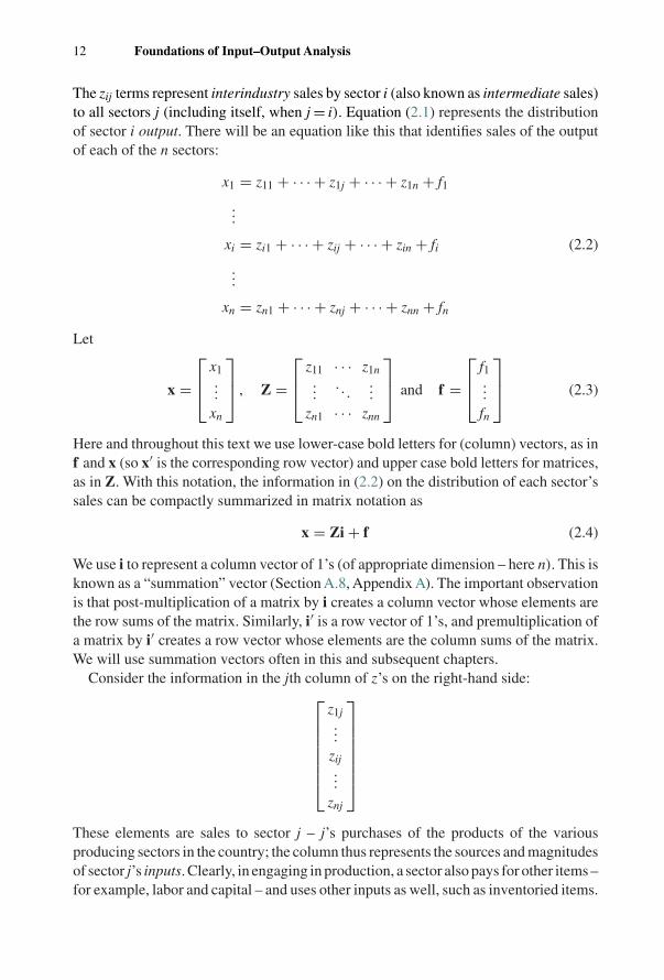
The zij terms represent interindustry sales by sector i (also known as intermediate sales)to all sectors j (including itself, when j = i). Equation (2.1) represents the distributionof sector i output. There will be an equation like this that identifies sales of the outputof each of the n sectors:
x1 = z11 + · · · + z1j + · · · + z1n + f1
...
xi = zi1 + · · · + zij + · · · + zin + fi (2.2)
...
xn = zn1 + · · · + znj + · · · + znn + fn
Let
x =⎡⎢⎣ x1
...xn
⎤⎥⎦ , Z =⎡⎢⎣ z11 · · · z1n
.... . .
...zn1 · · · znn
⎤⎥⎦ and f =⎡⎢⎣ f1
...fn
⎤⎥⎦ (2.3)
Here and throughout this text we use lower-case bold letters for (column) vectors, as inf and x (so x′ is the corresponding row vector) and upper case bold letters for matrices,as in Z. With this notation, the information in (2.2) on the distribution of each sector’ssales can be compactly summarized in matrix notation as
x = Zi + f (2.4)
We use i to represent a column vector of 1’s (of appropriate dimension – here n). This isknown as a “summation” vector (Section A.8, Appendix A). The important observationis that post-multiplication of a matrix by i creates a column vector whose elements arethe row sums of the matrix. Similarly, i′ is a row vector of 1’s, and premultiplication ofa matrix by i′ creates a row vector whose elements are the column sums of the matrix.We will use summation vectors often in this and subsequent chapters.
Consider the information in the jth column of z’s on the right-hand side:⎡⎢⎢⎢⎢⎢⎢⎣z1j...
zij...
znj
⎤⎥⎥⎥⎥⎥⎥⎦These elements are sales to sector j – j’s purchases of the products of the variousproducing sectors in the country; the column thus represents the sources and magnitudesof sector j’s inputs. Clearly, in engaging in production, a sector also pays for other items –for example, labor and capital – and uses other inputs as well, such as inventoried items.
2.2 Notation and Fundamental Relationships 13
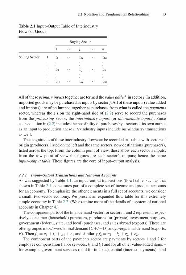
Table 2.1 Input–Output Table of InterindustryFlows of Goods
Buying Sector
1 · · · j · · · n
Selling Sector 1 z11 · · · z1j · · · z1n...
......
...i zi1 · · · zij · · · zin...
......
...n zn1 · · · znj · · · znn
All of these primary inputs together are termed the value added in sector j. In addition,imported goods may be purchased as inputs by sector j. All of these inputs (value addedand imports) are often lumped together as purchases from what is called the paymentssector, whereas the z’s on the right-hand side of (2.2) serve to record the purchasesfrom the processing sector, the interindustry inputs (or intermediate inputs). Sinceeach equation in (2.2) includes the possibility of purchases by a sector of its own outputas an input to production, these interindustry inputs include intraindustry transactionsas well.
The magnitudes of these interindustry flows can be recorded in a table, with sectors oforigin (producers) listed on the left and the same sectors, now destinations (purchasers),listed across the top. From the column point of view, these show each sector’s inputs;from the row point of view the figures are each sector’s outputs; hence the nameinput–output table. These figures are the core of input–output analysis.
2.2.1 Input–Output Transactions and National AccountsAs was suggested by Table 1.1, an input–output transactions (flow) table, such as thatshown in Table 2.1, constitutes part of a complete set of income and product accountsfor an economy. To emphasize the other elements in a full set of accounts, we considera small, two-sector economy. We present an expanded flow table for this extremelysimple economy in Table 2.2. (We examine more of the details of a system of nationalaccounts in Chapter 4.)
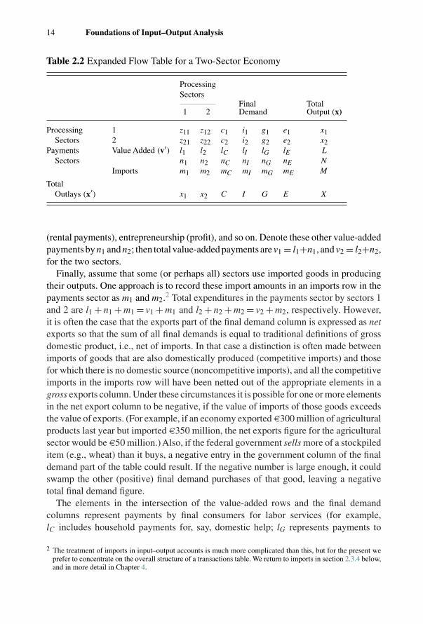
The component parts of the final demand vector for sectors 1 and 2 represent, respec-tively, consumer (household) purchases, purchases for (private) investment purposes,government (federal, state, and local) purchases, and sales abroad (exports). These areoften grouped into domestic final demand (C+I+G) and foreign final demand (exports,E). Then f1 = c1 + i1 + g1 + e1 and similarly f2 = c2 + i2 + g2 + e2.
The component parts of the payments sector are payments by sectors 1 and 2 foremployee compensation (labor services, l1 and l2) and for all other value-added items –for example, government services (paid for in taxes), capital (interest payments), land
14 Foundations of Input–Output Analysis
Table 2.2 Expanded Flow Table for a Two-Sector Economy
ProcessingSectors
Final Total1 2 Demand Output (x)
Processing 1 z11 z12 c1 i1 g1 e1 x1Sectors 2 z21 z22 c2 i2 g2 e2 x2
Payments Value Added (v′) l1 l2 lC lI lG lE LSectors n1 n2 nC nI nG nE N
Imports m1 m2 mC mI mG mE M
TotalOutlays (x′) x1 x2 C I G E X
(rental payments), entrepreneurship (profit), and so on. Denote these other value-addedpayments by n1 and n2; then total value-added payments are v1 = l1+n1, and v2 = l2+n2,for the two sectors.
Finally, assume that some (or perhaps all) sectors use imported goods in producingtheir outputs. One approach is to record these import amounts in an imports row in thepayments sector as m1 and m2.2 Total expenditures in the payments sector by sectors 1and 2 are l1 + n1 + m1 = v1 + m1 and l2 + n2 + m2 = v2 + m2, respectively. However,it is often the case that the exports part of the final demand column is expressed as netexports so that the sum of all final demands is equal to traditional definitions of grossdomestic product, i.e., net of imports. In that case a distinction is often made betweenimports of goods that are also domestically produced (competitive imports) and thosefor which there is no domestic source (noncompetitive imports), and all the competitiveimports in the imports row will have been netted out of the appropriate elements in agross exports column. Under these circumstances it is possible for one or more elementsin the net export column to be negative, if the value of imports of those goods exceedsthe value of exports. (For example, if an economy exported d300 million of agriculturalproducts last year but imported d350 million, the net exports figure for the agriculturalsector would be d50 million.) Also, if the federal government sells more of a stockpileditem (e.g., wheat) than it buys, a negative entry in the government column of the finaldemand part of the table could result. If the negative number is large enough, it couldswamp the other (positive) final demand purchases of that good, leaving a negativetotal final demand figure.
The elements in the intersection of the value-added rows and the final demandcolumns represent payments by final consumers for labor services (for example,lC includes household payments for, say, domestic help; lG represents payments to
2 The treatment of imports in input–output accounts is much more complicated than this, but for the present weprefer to concentrate on the overall structure of a transactions table. We return to imports in section 2.3.4 below,and in more detail in Chapter 4.
2.2 Notation and Fundamental Relationships 15
government workers) and for other value added (for example, nC includes tax paymentsby households). In the imports row and final demand columns are, for example, mG,which represents government purchases of imported items, and mE , which representsimported items that are re-exported.
Summing down the total output column, total gross output throughout the economy,X , is found as
X = x1 + x2 + L + N + M
This same value can be found by summing across the total outlays row; namely
X = x1 + x2 + C + I + G + E
These are simply two alternative ways of summing all the elements in the table.In national income and product accounting, it is the value of total final product that
is of interest – goods available for consumption, export, and so on. Equating the twoexpressions for X and subtracting x1 and x2 from both sides leaves
L + M + N = C + I + G + E
orL + N = C + I + G + (E − M )
The left-hand side represents gross national income – the total factor payments in theeconomy – and the right-hand side represents gross national product – the total spenton consumption and investment goods, total government purchases, and the total valueof net exports from the economy. Again, national accounts are examined in more detailin Chapter 4.
In most developed economies, consumption is the largest individual component offinal demand. For example, in the USA in 2003 the percentages of total final demandwere as follows: personal consumption expenditure (PCE), 71 percent; gross privatedomestic investment (including producers’ durable equipment, plant construction, res-idential construction, and net inventory change), 15 percent; government purchases(federal, state and local), 19 percent; net foreign exports, −5 percent (the value ofimports exceeded the value of exports). [However, in the USA during the 1942–1945period (World War II), PCE was between 40 and 48 percent and for much of the 1950sand 1960s it was under 60 percent.]
2.2.2 Production Functions and the Input–Output ModelIn input–output work, a fundamental assumption is that the interindustry flows fromi to j – recall that these are for a given period, say a year – depend entirely on thetotal output of sector j for that same time period. Clearly, no one would argue againstthe idea that the more cars produced in a year, the more steel will be needed duringthat year by automobile producers. Where argument does arise is over the exact natureof this relationship. In input–output analysis it is as follows: Given zij and xj – forexample, input of aluminum (i) bought by aircraft producers (j) last year and total
16 Foundations of Input–Output Analysis
aircraft production last year – form the ratio of aluminum input to aircraft output, zij/xj
[the units are ($/$)], and denote it by aij:
aij = zij
xj= value of aluminum bought by aircraft producers last year
value of aircraft production last year(2.5)
This ratio is called a technical coefficient; the terms input–output coefficient anddirect input coefficient are also often used. For example, if z14 = $300 and x4 = $15, 000(sector 4 used $300 of goods from sector 1 in producing $15,000 of sector 4 output),a14 = z14/x4 = $300/$15, 000 = 0.02. Since a14 is actually $0.02/$1, the 0.02 is inter-preted as the “dollars’ worth of inputs from sector 1 per dollar’s worth of output ofsector 4.”
From (2.5), aijxj = zij. This is trivial algebra, but it presents the operational formin which the technical coefficients are used. In input–output analysis, once a set ofobservations has given us the result a14 = 0.02, this technical coefficient is assumed tobe unchanging in the sense that if one asked how much sector 4 would buy from sector1 if sector 4 were to produce a total output (x4) of $45,000, the input–output answerwould be z14 = a14x4 = (0.02)($45, 000)= $900 – when output of sector 4 is tripled,the input from sector 1 is tripled. The aij are viewed as measuring fixed relationshipsbetween a sector’s output and its inputs. Economies of scale in production are thusignored; production in a Leontief system operates under what is known as constantreturns to scale.
In addition, input–output analysis requires that a sector use inputs in fixed pro-portions. Suppose, to continue the previous example, that sector 4 also buysinputs from sector 2, and that, for the period of observation, z24 = $750. There-fore a24 = z24/x4 = $750/$15, 000 = 0.05. For x4 = $15, 000, inputs from sector 1and from sector 2 were used in the proportion p12 = z14/z24 = $300/$750 = 0.4.If x4 were $45,000, z24 would be (0.05)($45,000) = $2250; since z14 = $900 forx4 = $45, 000, the proportion between inputs from sector 1 and from sector 2 is$900/$2250 = 0.4, as before. This reflects the fact that
p12 = z14/z24 = a14x4/a24x4 = a14/a24 = 0.02/0.05 = 0.4;
the proportion is the ratio of the technical coefficients, and since the coefficients arefixed, then the input proportion is fixed.
For the reader with some background in basic microeconomics, we can identify theform of production function inherent in the input–output system and compare it withthat in the general neoclassical microeconomic approach. Production functions relatethe amounts of inputs used by a sector to the maximum amount of output that could beproduced by that sector with those inputs. An illustration is
xj = f (z1j, z2j, . . . , znj, vj, mj)
2.2 Notation and Fundamental Relationships 17
Using the definition of the technical coefficients in (2.5), we can see that in the Leontiefmodel this becomes
xj = z1j
a1j= z2j
a2j= · · · = znj
anj
(This ignores, for the moment, the contributions of vj and mj.)A problem with this extremely simple formulation is that it is meaningless if a par-
ticular input i is not used in production of j, since then aij = 0 and hence zij/aij isinfinitely large. Thus, the more usual specification of the kind of production functionthat is embodied in the input–output model is
xj = min
(z1j
a1j,
z2j
a2j, · · · ,
znj
anj
)where min (x, y, z) denotes the smallest of the numbers x, y and z. In the input–outputmodel, for those aij coefficients that are not zero, these ratios will all be the same, andequal to xj – from the fundamental definition of aij in (2.5). For those aij coefficientsthat are zero, the ratio zij/aij will be infinitely large and hence will be overlookedin the process of searching for the smallest among the ratios. This specification ofthe production function in the input–output model reflects the assumption of constantreturns to scale; multiplication of z1j, z2j, . . . , znj by any constant will multiply xj by thesame constant. (Tripling all inputs will triple output; cutting inputs in half will halveoutput, etc.)
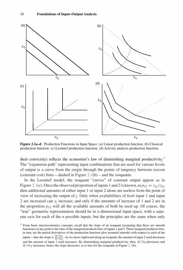
For the reader who is acquainted with the economist’s production function geom-etry, we show four alternative representations of production functions in input spacefor a two-sector economy in Figure 2.1. A linear production function, depicted inFigure 2.1(a) assumes that output is a simple linear function of inputs, which meansthat the inputs are infinitely substitutable for each other for any level of output. Thefigure shows a set of isoquants (constant output lines) depicting higher and higher levelsof output.
A classical production function, depicted in Figure 2.1(b), also shows a set of iso-quants (now constant output curves) depicting higher and higher levels of output. Fora given value of z1j in Figure 2.1(b), increasing z2j leads to increases in xj – intersec-tions with higher-value isoquants. In this case input substitution is also possible butnot linearly, as indicated by the isoquants showing alternative input combinations thatgenerate the same level of output. For example, moving rightward along a particularisoquant in Figure 2.1(b) can be accomplished by reducing the amount of input 2 andincreasing the amount of input 1, or leftward by reducing z1j and increasing z2j.
The shape of the isoquants in Figure 2.1(b) reflects two specific classical assumptionsabout how inputs are combined to produce outputs. The negative slopes of the isoquantsrepresent the fact that as the amount of one input is decreased, the amount of the otherinput must be increased in order to maintain the level of production indicated by aspecific isoquant. The fact that the curves bulge toward the origin (mathematically
18 Foundations of Input–Output Analysis
z2j
z1j
(a)
z2j
z1j
(b)
z2j
z1j
(c)
z2j
z1j
(d)
Figure 2.1a–d. Production Functions in Input Space. (a) Linear production function. (b) Classicalproduction function. (c) Leontief production function. (d) Activity analysis production function.
their convexity) reflects the economist’s law of diminishing marginal productivity.3
The “expansion path” representing input combinations that are used for various levelsof output is a curve from the origin through the points of tangency between isocost(constant cost) lines – dashed in Figure 2.1(b) – and the isoquants.
In the Leontief model, the isoquant “curves” of constant output appear as inFigure 2.1(c). Once the observed proportion of inputs 1 and 2 is known, as p12 = z1j/z2j,then additional amounts of either input 1 or input 2 alone are useless from the point ofview of increasing the output of j. Only when availabilities of both input 1 and input2 are increased can xj increase; and only if the amounts of increase of 1 and 2 are inthe proportion p12 will all the available amounts of both be used up. Of course, the“true” geometric representation should be in n-dimensional input space, with a sepa-rate axis for each of the n possible inputs, but the principles are the same when only
3 From basic microeconomics concepts, recall that the slope of an isoquant (assuming that these are smoothfunctions) at any point is the ratio of the marginal productivities of inputs 1 and 2. These marginal productivities,in turn, are the partial derivatives of the production function (also assumed smooth) with respect to each of the
inputs – thus the slope is ∂f /∂x1∂f /∂x2
. As we move rightward along an isoquant, the amount of input 2 used decreases
and the amount of input 1 used increases. By diminishing marginal productivity, then, ∂f /∂x1decreases and∂f /∂x2 increases; hence the slope decreases, as is true for the isoquants in Figure 2.1(b).
2.2 Notation and Fundamental Relationships 19
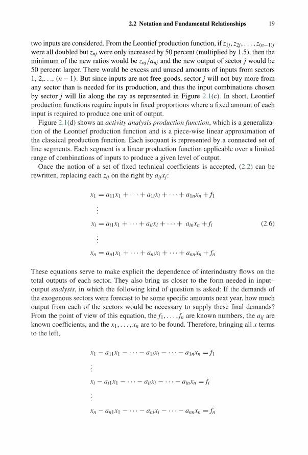
two inputs are considered. From the Leontief production function, if z1j, z2j, . . . , z(n−1)j
were all doubled but znj were only increased by 50 percent (multiplied by 1.5), then theminimum of the new ratios would be znj/anj and the new output of sector j would be50 percent larger. There would be excess and unused amounts of inputs from sectors1, 2,. . ., (n − 1). But since inputs are not free goods, sector j will not buy more fromany sector than is needed for its production, and thus the input combinations chosenby sector j will lie along the ray as represented in Figure 2.1(c). In short, Leontiefproduction functions require inputs in fixed proportions where a fixed amount of eachinput is required to produce one unit of output.
Figure 2.1(d) shows an activity analysis production function, which is a generaliza-tion of the Leontief production function and is a piece-wise linear approximation ofthe classical production function. Each isoquant is represented by a connected set ofline segments. Each segment is a linear production function applicable over a limitedrange of combinations of inputs to produce a given level of output.
Once the notion of a set of fixed technical coefficients is accepted, (2.2) can berewritten, replacing each zij on the right by aijxj:
x1 = a11x1 + · · · + a1ixi + · · · + a1nxn + f1
...
xi = ai1x1 + · · · + aiixi + · · · + ainxn + fi (2.6)
...
xn = an1x1 + · · · + anixi + · · · + annxn + fn
These equations serve to make explicit the dependence of interindustry flows on thetotal outputs of each sector. They also bring us closer to the form needed in input–output analysis, in which the following kind of question is asked: If the demands ofthe exogenous sectors were forecast to be some specific amounts next year, how muchoutput from each of the sectors would be necessary to supply these final demands?From the point of view of this equation, the f1, . . . , fn are known numbers, the aij areknown coefficients, and the x1, . . . , xn are to be found. Therefore, bringing all x termsto the left,
x1 − a11x1 − · · · − a1ixi − · · · − a1nxn = f1
...
xi − ai1x1 − · · · − aiixi − · · · − ainxn = fi
...
xn − an1x1 − · · · − anixi − · · · − annxn = fn
20 Foundations of Input–Output Analysis
and, grouping the x1 together in the first equation, the x2 in the second, and so on,
(1 − a11)x1 − · · · − a1ixi − · · · − a1nxn = f1
...
− ai1x1 − · · · + (1 − aii)xi − · · · − ainxn = fi (2.7)
...
− an1x1 − · · · − anixi − · · · + (1 − ann)xn = fn
These relationships can be represented compactly in matrix form. In matrix algebranotation, a “hat” over a vector denotes a diagonal matrix with the elements of the
vector along the main diagonal, so, for example, x =⎡⎢⎣ x1 · · · 0
.... . .
...0 · · · xn
⎤⎥⎦. From the basic
definition of an inverse, (x)(x)−1 = I, it follows that x−1 =⎡⎢⎣ 1/x1 · · · 0
.... . .
...0 · · · 1/xn
⎤⎥⎦. Also,
postmultiplication of a matrix, M, by a diagonal matrix, d, creates a matrix in whicheach element in column j of M is multiplied by dj in d (Appendix A, section A.7).Therefore the n × n matrix of technical coefficients can be represented as
A = Zx−1 (2.8)
Using the definitions in (2.3) and (2.8), the matrix expression for (2.6) is
x = Ax + f (2.9)
Let I be the n × n identity matrix – ones on the main diagonal and zeros elsewhere;
I =⎡⎢⎣ 1 · · · 0
.... . .
...0 · · · 1
⎤⎥⎦ so then (I − A) =
⎡⎢⎢⎢⎣(1 − a11) −a12 · · · −a1n
−a21 (1 − a22) · · · −a2n...
.... . .
...−an1 −an2 · · · (1 − ann)
⎤⎥⎥⎥⎦ .
Then the complete n × n system shown in (2.7) is just4
(I − A)x = f (2.10)
For a given set of f ’s, this is a set of n linear equations in the n unknowns, x1, x2, . . . , xn
and hence it may or may not be possible to find a unique solution. In fact, whether or
4 This is parallel to the form Ax = b that is usually used to denote a set of linear equations. The difference ispurely notational; since it is standard in input–output analysis to define the technical coefficients matrix as A,then the matrix of coefficients in the input–output equation system becomes (I − A). Similarly, convention isresponsible for denoting the right-hand sides of the input–output equations by f (for final demand) instead of b.
2.3 An Illustration of Input–Output Calculations 21
not there is a unique solution depends on whether or not (I − A) is singular; that is,whether or not (I − A)−1 exists. The matrix A is known as the technical (or input–output, or direct input) coefficients matrix. From the basic definition of an inverse for asquare matrix (Appendix A), (I − A)−1 = (1/ |I − A|)[adj(I − A)]. If |I − A| �= 0, then(I − A)−1 can be found, and using standard matrix algebra results for linear equationsthe unique solution to (2.10) is given by
x = (I − A)−1f = Lf (2.11)
where (I − A)−1 = L = [lij] is known as the Leontief inverse or the total requirementsmatrix.
In more detail, the equations summarized in (2.11) are
x1 = l11f1 + · · · + l1jfj + · · · + l1nfn...xi = li1f1 + · · · + lijfj + · · · + linfn...xn = ln1f1 + · · · + lnjfj + · · · + lnnfn
(2.12)
This makes clear the dependence of each of the gross outputs on the values of each ofthe final demands. Readers familiar with differential calculus and partial derivativeswill recognize that ∂xi/∂fj = lij.
2.3 An Illustration of Input–Output Calculations
2.3.1 Numerical Example: Hypothetical Figures – Approach IImpacts on Industry Outputs We now turn to a small numerical example, as
presented in Table 2.3. For the moment, the final demand elements and the value-addedelements have not been disaggregated into their component parts.
The corresponding table of input–output coefficients, Table 2.4, is found by dividingeach flow in a particular column of the producing sectors in Table 2.3 by the totaloutput (row sum) of that sector. Thus, a11 = 150/1000 = 0.15; a21 = 200/1000 = 0.2;a12 = 500/2000 = 0.25; a22 = 100/2000 = 0.05. In particular,
A = Zx−1 =[
150 500200 100
] [1/1000 0
0 1/2000
]TheAmatrix is shown in Table 2.4. To add specificity for the remainder of this example,we assume sector 1 represents “Agriculture” and sector 2 “Manufacturing.”
The principal way in which input–output coefficients are used for analysis is as fol-lows. We assume that the numbers in Table 2.4 represent the structure of production inthe economy; the columns are, in effect, the production recipes for each of the sectors,in terms of inputs from all the sectors. To produce one dollar’s worth of manufacturedgoods, for example, 25 cents’ worth of agricultural products and 5 cents’ worth of
22 Foundations of Input–Output Analysis
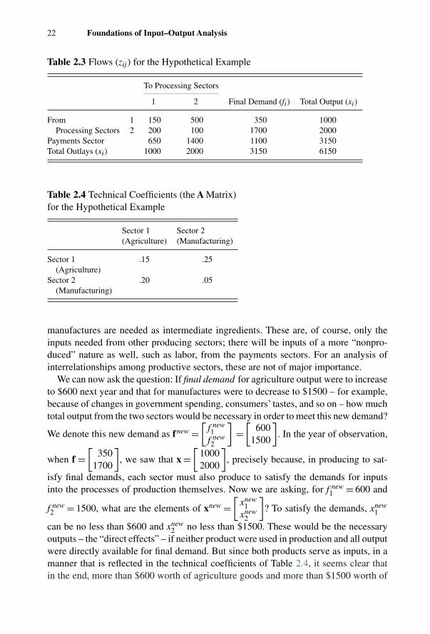
Table 2.3 Flows (zij) for the Hypothetical Example
To Processing Sectors
1 2 Final Demand (fi) Total Output (xi)
From 1 150 500 350 1000Processing Sectors 2 200 100 1700 2000
Payments Sector 650 1400 1100 3150Total Outlays (xi) 1000 2000 3150 6150
Table 2.4 Technical Coefficients (the A Matrix)for the Hypothetical Example
Sector 1 Sector 2(Agriculture) (Manufacturing)
Sector 1 .15 .25(Agriculture)
Sector 2 .20 .05(Manufacturing)
manufactures are needed as intermediate ingredients. These are, of course, only theinputs needed from other producing sectors; there will be inputs of a more “nonpro-duced” nature as well, such as labor, from the payments sectors. For an analysis ofinterrelationships among productive sectors, these are not of major importance.
We can now ask the question: If final demand for agriculture output were to increaseto $600 next year and that for manufactures were to decrease to $1500 – for example,because of changes in government spending, consumers’ tastes, and so on – how muchtotal output from the two sectors would be necessary in order to meet this new demand?
We denote this new demand as fnew =[
f new1
f new2
]=[
6001500
]. In the year of observation,
when f =[
3501700
], we saw that x =
[10002000
], precisely because, in producing to sat-
isfy final demands, each sector must also produce to satisfy the demands for inputsinto the processes of production themselves. Now we are asking, for f new
1 = 600 and
f new2 = 1500, what are the elements of xnew =
[xnew
1xnew
2
]? To satisfy the demands, xnew
1
can be no less than $600 and xnew2 no less than $1500. These would be the necessary
outputs – the “direct effects” – if neither product were used in production and all outputwere directly available for final demand. But since both products serve as inputs, in amanner that is reflected in the technical coefficients of Table 2.4, it seems clear thatin the end, more than $600 worth of agriculture goods and more than $1500 worth of
2.3 An Illustration of Input–Output Calculations 23
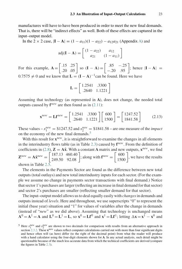
manufactures will have to have been produced in order to meet the new final demands.That is, there will be “indirect effects” as well. Both of these effects are captured in theinput–output model.
In the 2 × 2 case, |I − A| = (1 − a11)(1 − a22) − a12a21 (Appendix A) and
adj(I − A) =[
(1 − a22) a12
a21 (1 − a11)
]
For this example, A =[
.15 .25
.20 .05
]so (I − A) =
[.85 −.25
−.20 .95
]; hence |I − A| =
0.7575 �= 0 and we know that L = (I − A)−1can be found. Here we have
L =[
1.2541 .3300.2640 1.1221
]Assuming that technology (as represented in A), does not change, the needed totaloutputs caused by fnew are then found as in (2.11):
xnew = Lfnew =[
1.2541 .3300.2640 1.1221
] [600
1500
]=[
1247.521841.58
](2.13)
These values – xnew1 = $1247.52 and xnew
2 = $1841.58 – are one measure of the impacton the economy of the new final demands.5
With this result for xnew, it is straightforward to examine the changes in all elementsin the interindustry flows table (as in Table 2.3) caused by fnew. From the definition ofcoefficients in (2.8), Z = Ax. With a constant A matrix and new outputs, xnew, we find
Znew = Axnew =[
187.13 460.40249.50 92.08
]; along with fnew =
[600
1500
], we have the results
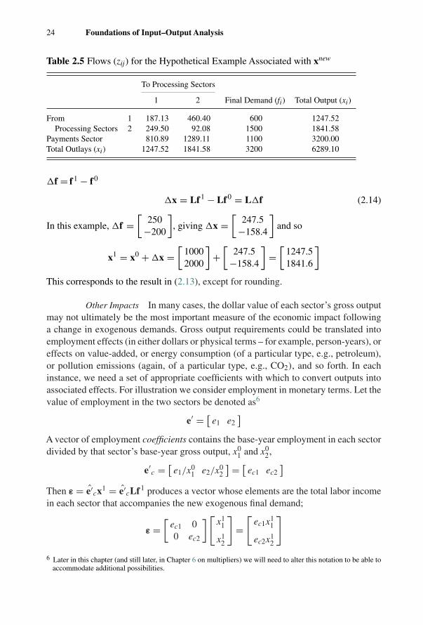
shown in Table 2.5.The elements in the Payments Sector are found as the difference between new total
outputs (total outlays) and new total interindustry inputs for each sector. (For the exam-ple we assume no change in payments sector transactions with final demand.) Noticethat sector 1’s purchases are larger (reflecting an increase in final demand for that sector)and sector 2’s purchases are smaller (reflecting smaller demand for that sector).
The input–output model allows us to deal equally easily with changes in demands andoutputs instead of levels. Here and throughout, we use superscripts “0” to represent theinitial (base year) situation and “1” for values of variables after the change in demands(instead of “new” as we did above). Assuming that technology is unchanged meansA0 = A1 = A and L0 = L1 = L, so x0 = Lf0 and x1 = Lf1; letting �x = x1 − x0 and
5 Here xnew1 and xnew
2 are shown to two decimals for comparison with results from an alternative approach insection 2.3.2. These xnew values reflect computer calculations carried out with more than four significant digitsand hence often will (as here) differ (to the right of the decimal point) from what the reader will producewith a hand calculator using the four-digit elements shown for A. In any actual analysis, such detail might bequestionable because of the much less accurate data from which the technical coefficients are derived (comparethe figures in Table 2.3).
24 Foundations of Input–Output Analysis
Table 2.5 Flows (zij) for the Hypothetical Example Associated with xnew
To Processing Sectors
1 2 Final Demand (fi) Total Output (xi)
From 1 187.13 460.40 600 1247.52Processing Sectors 2 249.50 92.08 1500 1841.58
Payments Sector 810.89 1289.11 1100 3200.00Total Outlays (xi) 1247.52 1841.58 3200 6289.10
�f = f1 − f0
�x = Lf1 − Lf0 = L�f (2.14)
In this example, �f =[
250−200
], giving �x =
[247.5
−158.4
]and so
x1 = x0 + �x =[
10002000
]+[
247.5−158.4
]=[
1247.51841.6
]This corresponds to the result in (2.13), except for rounding.
Other Impacts In many cases, the dollar value of each sector’s gross outputmay not ultimately be the most important measure of the economic impact followinga change in exogenous demands. Gross output requirements could be translated intoemployment effects (in either dollars or physical terms – for example, person-years), oreffects on value-added, or energy consumption (of a particular type, e.g., petroleum),or pollution emissions (again, of a particular type, e.g., CO2), and so forth. In eachinstance, we need a set of appropriate coefficients with which to convert outputs intoassociated effects. For illustration we consider employment in monetary terms. Let thevalue of employment in the two sectors be denoted as6
e′ = [e1 e2
]A vector of employment coefficients contains the base-year employment in each sectordivided by that sector’s base-year gross output, x0
1 and x02,
e′c = [
e1/x01 e2/x0
2
] = [ec1 ec2
]Then ε = e′
cx1 = e′cLf1 produces a vector whose elements are the total labor income
in each sector that accompanies the new exogenous final demand;
ε =[
ec1 00 ec2
][ x11
x12
]=[
ec1x11
ec2x12
]6 Later in this chapter (and still later, in Chapter 6 on multipliers) we will need to alter this notation to be able to
accommodate additional possibilities.
2.3 An Illustration of Input–Output Calculations 25
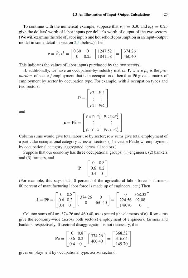
To continue with the numerical example, suppose that ec1 = 0.30 and ec2 = 0.25give the dollars’ worth of labor inputs per dollar’s worth of output of the two sectors.(We will examine the role of labor inputs and household consumption in an input–outputmodel in some detail in section 2.5, below.) Then
ε = e′cx1 =
[0.30 0
0 0.25
] [1247.521841.58
]=[
374.26460.40
]This indicates the values of labor inputs purchased by the two sectors.
If, additionally, we have an occupation-by-industry matrix, P, where pij is the pro-portion of sector j employment that is in occupation i, then ε = Pε gives a matrix ofemployment by sector by occupation type. For example, with k occupation types andtwo sectors,
P =⎡⎢⎣ p11 p12
......
pk1 pk2
⎤⎥⎦and
ε = Pε =⎡⎢⎣ p11ec1x1
1 p12ec2x12
......
pk1ec1x11 pk2ec2x1
2
⎤⎥⎦Column sums would give total labor use by sector; row sums give total employment ofa particular occupational category across all sectors. (The vector Pε shows employmentby occupational category, aggregated across all sectors.)
Suppose that our economy has three occupational groups: (1) engineers, (2) bankersand (3) farmers, and
P =⎡⎣ 0 0.8
0.6 0.20.4 0
⎤⎦(For example, this says that 40 percent of the agricultural labor force is farmers;80 percent of manufacturing labor force is made up of engineers, etc.) Then
ε = Pε =⎡⎣ 0 0.8
0.6 0.20.4 0
⎤⎦[374.26 0
0 460.40
]=⎡⎣ 0 368.32
224.56 92.08149.70 0
⎤⎦Column sums of ε are 374.26 and 460.40, as expected (the elements of ε). Row sums
give the economy-wide (across both sectors) employment of engineers, farmers andbankers, respectively. If sectoral disaggregation is not necessary, then
Pε =⎡⎣ 0 0.8
0.6 0.20.4 0
⎤⎦[374.26460.40
]=⎡⎣ 368.32
316.64149.70
⎤⎦gives employment by occupational type, across sectors.

26 Foundations of Input–Output Analysis
A wide variety of such conversion coefficients vectors (as in e′c) or matrices (as in
P) is possible. For example, in arid regions, water-use coefficients, w′c = [
wc1 wc2],
could be used in w′cx′ to assess the water consumption associated with new outputs
generated by new final demands. We explore these kinds of alternative impacts againin Chapter 6 on input–output multipliers, and in Chapters 9 and 10, some of the energyand environmental repercussions of final demand impacts are discussed in detail.
2.3.2 Numerical Example: Hypothetical Figures – Approach IIConsider the same economy, whose 2 × 2 technical coefficients matrix is given in
Table 2.4 and for which the projected f1 vector is
[600
1500
]. We can examine the question
of outputs necessary to satisfy this final demand in a more intuitive way that is lessmechanical than finding elements in an inverse matrix.
1. Initially, it is clear that agriculture needs to produce $600 and manufacturing, $1500.If the sectors are going to meet the new final demands, they could not get away withproducing less than these amounts.
2. However, to produce $600, agriculture needs, as inputs to that productive process,(0.15)($600) = $90 from itself and (0.20)($600) = $120 from manufacturing. Thesefigures come from the coefficients in column 1 of the A matrix – the productionrecipe for agriculture. Similarly, to produce its $1500, manufacturing will have tobuy (0.25)($1500)= $375 from agriculture and (0.05)($1500) = $75 from itself.Thus agriculture must, in fact, produce the $600 noted in 1, above, plus another$(90 + 375) = $465 more, to satisfy the needs for inputs that it has itself and alsothat come from manufacturing. Similarly, manufacturing will have to produce anadditional $(120 + 75) = $195 to satisfy its own need plus that of agriculture forinputs to produce the “original” $600 and $1500.
3. In item 2, above, we found the interindustry needs that resulted from productionof $600 in agriculture and $1500 in manufacturing. These were $465 and $195,respectively. But now we realize that this “extra” production, above the $600 and$1500, will also generate interindustry needs – in order to engage in the produc-tion of $465, agriculture will need (0.15)($465) = $69.75 from itself and (0.20)($465) = $93 from manufacturing. Similarly, manufacturing will now additionallyneed (.025)($195) = $48.75 from agriculture and (0.05)($195) = $9.75 from itself.The total new demands for the two sectors are thus $(69.75 + 48.75) = $118.50 and$(93 + 9.75) = $102.75.
4. At this point we realize that it is necessary to treat the additional $118.50 for agri-culture and $102.75 for manufacturing in the same fashion as the $465 and $195 initem 3. Hence we find additional required outputs of $43.46 and $28.84 from thetwo sectors.
5. Continuing in this way, we find that eventually the numbers become so small thatthey can be ignored (less than $0.005).
2.3 An Illustration of Input–Output Calculations 27
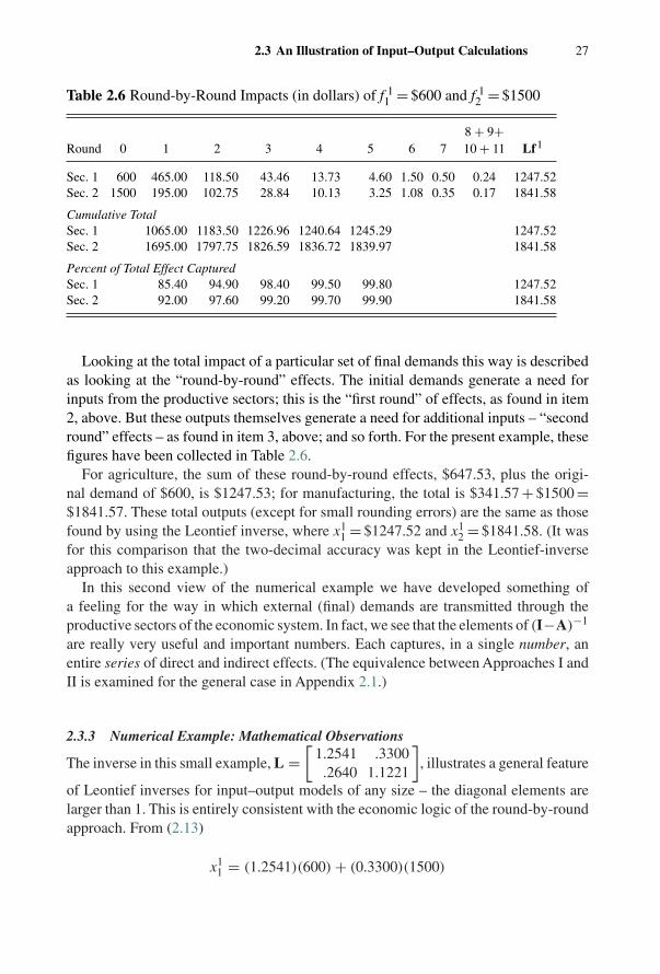
Table 2.6 Round-by-Round Impacts (in dollars) of f 11 = $600 and f 1
2 = $1500
8 + 9+Round 0 1 2 3 4 5 6 7 10 + 11 Lf1
Sec. 1 600 465.00 118.50 43.46 13.73 4.60 1.50 0.50 0.24 1247.52Sec. 2 1500 195.00 102.75 28.84 10.13 3.25 1.08 0.35 0.17 1841.58
Cumulative TotalSec. 1 1065.00 1183.50 1226.96 1240.64 1245.29 1247.52Sec. 2 1695.00 1797.75 1826.59 1836.72 1839.97 1841.58
Percent of Total Effect CapturedSec. 1 85.40 94.90 98.40 99.50 99.80 1247.52Sec. 2 92.00 97.60 99.20 99.70 99.90 1841.58
Looking at the total impact of a particular set of final demands this way is describedas looking at the “round-by-round” effects. The initial demands generate a need forinputs from the productive sectors; this is the “first round” of effects, as found in item2, above. But these outputs themselves generate a need for additional inputs – “secondround” effects – as found in item 3, above; and so forth. For the present example, thesefigures have been collected in Table 2.6.
For agriculture, the sum of these round-by-round effects, $647.53, plus the origi-nal demand of $600, is $1247.53; for manufacturing, the total is $341.57 + $1500 =$1841.57. These total outputs (except for small rounding errors) are the same as thosefound by using the Leontief inverse, where x1
1 = $1247.52 and x12 = $1841.58. (It was
for this comparison that the two-decimal accuracy was kept in the Leontief-inverseapproach to this example.)
In this second view of the numerical example we have developed something ofa feeling for the way in which external (final) demands are transmitted through theproductive sectors of the economic system. In fact, we see that the elements of (I−A)−1
are really very useful and important numbers. Each captures, in a single number, anentire series of direct and indirect effects. (The equivalence between Approaches I andII is examined for the general case in Appendix 2.1.)
2.3.3 Numerical Example: Mathematical Observations
The inverse in this small example, L =[
1.2541 .3300.2640 1.1221
], illustrates a general feature
of Leontief inverses for input–output models of any size – the diagonal elements arelarger than 1. This is entirely consistent with the economic logic of the round-by-roundapproach. From (2.13)
x11 = (1.2541)(600) + (0.3300)(1500)
28 Foundations of Input–Output Analysis
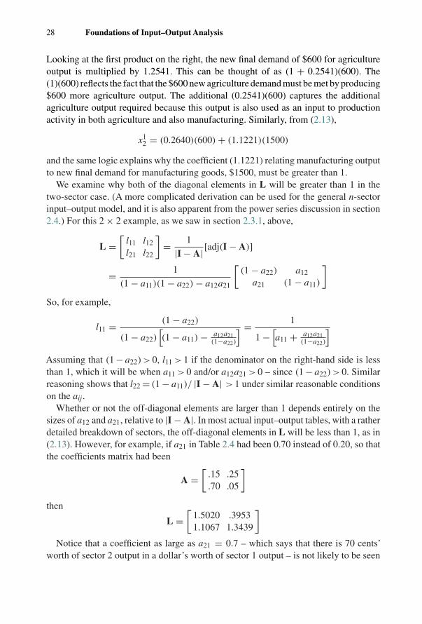
Looking at the first product on the right, the new final demand of $600 for agricultureoutput is multiplied by 1.2541. This can be thought of as (1 + 0.2541)(600). The(1)(600) reflects the fact that the $600 new agriculture demand must be met by producing$600 more agriculture output. The additional (0.2541)(600) captures the additionalagriculture output required because this output is also used as an input to productionactivity in both agriculture and also manufacturing. Similarly, from (2.13),
x12 = (0.2640)(600) + (1.1221)(1500)
and the same logic explains why the coefficient (1.1221) relating manufacturing outputto new final demand for manufacturing goods, $1500, must be greater than 1.
We examine why both of the diagonal elements in L will be greater than 1 in thetwo-sector case. (A more complicated derivation can be used for the general n-sectorinput–output model, and it is also apparent from the power series discussion in section2.4.) For this 2 × 2 example, as we saw in section 2.3.1, above,
L =[
l11 l12
l21 l22
]= 1
|I − A| [adj(I − A)]
= 1
(1 − a11)(1 − a22) − a12a21
[(1 − a22) a12
a21 (1 − a11)
]So, for example,
l11 = (1 − a22)
(1 − a22)[(1 − a11) − a12a21
(1−a22)
] = 1
1 −[a11 + a12a21
(1−a22)
]Assuming that (1 − a22) > 0, l11 > 1 if the denominator on the right-hand side is lessthan 1, which it will be when a11 > 0 and/or a12a21 > 0 – since (1 − a22) > 0. Similarreasoning shows that l22 = (1 − a11)/ |I − A| > 1 under similar reasonable conditionson the aij.
Whether or not the off-diagonal elements are larger than 1 depends entirely on thesizes of a12 and a21, relative to |I − A|. In most actual input–output tables, with a ratherdetailed breakdown of sectors, the off-diagonal elements in L will be less than 1, as in(2.13). However, for example, if a21 in Table 2.4 had been 0.70 instead of 0.20, so thatthe coefficients matrix had been
A =[
.15 .25
.70 .05
]then
L =[
1.5020 .39531.1067 1.3439
]Notice that a coefficient as large as a21 = 0.7 – which says that there is 70 cents’
worth of sector 2 output in a dollar’s worth of sector 1 output – is not likely to be seen
2.3 An Illustration of Input–Output Calculations 29
Table 2.7 The 2003 US Domestic Direct Requirements Matrix, A
Sector 1 2 3 4 5 6 7
1 Agriculture .2008 .0000 .0011 .0338 .0001 .0018 .00092 Mining .0010 .0658 .0035 .0219 .0151 .0001 .00263 Construction .0034 .0002 .0012 .0021 .0035 .0071 .02144 Manufacturing .1247 .0684 .1801 .2319 .0339 .0414 .07265 Trade, Transportation
& Utilities.0855 .0529 .0914 .0952 .0645 .0315 .0528
6 Services .0897 .1668 .1332 .1255 .1647 .2712 .18737 Other .0093 .0129 .0095 .0197 .0190 .0184 .0228
Table 2.8 The 2003 US Domestic Total Requirements Matrix, L = (I − A)−1
Sector 1 2 3 4 5 6 7
1 Agriculture 1.2616 .0058 .0131 .0576 .0037 .0069 .00722 Mining .0093 1.0748 .0122 .0343 .0193 .0033 .00733 Construction .0075 .0034 1.0047 .0064 .0065 .0111 .02504 Manufacturing .2292 .1192 .2615 1.3419 .0692 .0856 .12615 Trade, Transportation .1493 .0850 .1371 .1563 1.0887 .0598 .0853
& Utilities6 Services .2383 .2931 .2700 .2918 .2712 1.4116 .31387 Other .0243 .0239 .0231 .0367 .0280 .0297 1.0338
often in real tables. The sizes of the between-sector technical coefficients, aij (i �= j),and of the off-diagonal elements in L, are related to the level of sectoral detail (that is,the number of sectors) in the model. We will return to this topic in Chapter 4, whenwe consider the effects of aggregating (combining) sectors in an input–output model.(In Appendix 2.2 we examine the conditions under which a Leontief inverse matrixwill always contain only non-negative elements, as logic suggests should always be thecase.)
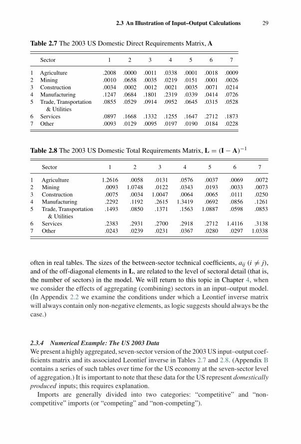
2.3.4 Numerical Example: The US 2003 DataWe present a highly aggregated, seven-sector version of the 2003 US input–output coef-ficients matrix and its associated Leontief inverse in Tables 2.7 and 2.8. (Appendix Bcontains a series of such tables over time for the US economy at the seven-sector levelof aggregation.) It is important to note that these data for the US represent domesticallyproduced inputs; this requires explanation.
Imports are generally divided into two categories: “competitive” and “non-competitive” imports (or “competing” and “non-competing”).

30 Foundations of Input–Output Analysis
Competitive imports are goods that have a domestic counterpart (that is, are alsoproduced in the USA). For example, grapes from Chile that are used to make grapejelly in the USA, where domestically grown grapes are also used in grape jelly recipes.
Non-competitive imports have no domestic counterpart. For example, coffee beansfrom Brazil used by US coffee roasting firms (coffee beans are not grown in the USA).
Some national tables (the USA is one example) show competitive imports within thetransactions table, so that sales of grapes to jelly producers include both domestic andforeign sources. This correctly reflects the total amount of grapes needed by domesticproducers. However, it causes problems when input–output models are used for impactanalysis. Briefly put, this is because an analyst is usually interested in the economicconsequences on the domestic (or regional or local) economy of an exogenous demandchange. With Chilean grapes in a transactions matrix, and hence in the associated Aand L matrices, some of the demand repercussions measured by the model wouldin fact be felt by Chilean grape growers. For this reason, we present here US databased on a domestic transactions matrix (ZD) in which the transactions matrix (Z) hasbeen purged of “competitive” (or “competing”) imports. In matrix terms, ZD = Z − M,where M is a matrix of competitive imports. This “scrubbing” of the matrix is notalways easy to do if the data are lumped together in a published Z table (as is thecase in the USA), but it is very important when the question is one of impacts offinal demand changes on the domestic economy (and this is usually the question ofinterest).7
Spending on non-competitive imports usually appears in a row in the paymentssector (a single value indicating a sector’s payments for all non-competitive imports).We return to these issues in Chapter 4.
The effects on US output of various final-demand vectors can be easily quanti-fied using L in Table 2.8. For example, suppose that there were increased foreigndemand (the export component of the final-demand vector) for agricultural and man-ufactured items of $1.2 million and $6.8 million, respectively. Here (in millions ofdollars)
�f =
⎡⎢⎢⎢⎢⎢⎢⎢⎢⎢⎢⎣
1.2
0
0
6.8
0
0
0
⎤⎥⎥⎥⎥⎥⎥⎥⎥⎥⎥⎦
7 By contrast, if one is interested in the structure of production (“production recipes”) and if or how they havechanged over time (structural analysis), it may be more useful to have competitive imports included in the Zmatrix and hence reflected in A and L, since such imports are certainly part of those recipes.
2.4 The Power Series Approximation of (I − A)−1 31
and, using (2.14), we find from L in Table 2.8 that (in millions of dollars)
�x =
⎡⎢⎢⎢⎢⎢⎢⎢⎢⎣
1.91140.24440.05269.12491.24212.27090.2788
⎤⎥⎥⎥⎥⎥⎥⎥⎥⎦As might be expected, the greatest effect, $9.125 million, is felt in the manufacturing
sector. The next-greatest effect, $2.271 million, is felt in services. Also, agricultureoutput would increase by $1.911 million and trade, transportation and utilities wouldincrease by $1.242 million. Effects on the remaining three sectors are less than $1million. The total new output effect throughout the country, obtained by summingthe elements in �x, is $15.125 million; this is generated by a total new exogenousdemand of $8 million. This again illustrates the multiplicative effect in an economyof an exogenous stimulus via an increase in one or more components of final demand.These multiplier effects will be discussed in further detail in Chapter 6.
2.4 The Power Series Approximation of (I − A)−1
In preparing input–output tables for many real-world applications of the model, in whichone wants to maintain a reasonable distinction between sectors (e.g., so that sectorsproducing aluminum storm windows and women’s apparel are not lumped togetheras a single sector labeled “manufacturing”), tables with hundreds of sectors are notunusual. However, early in the history of input–output studies, computer speed andcapacity posed real problems for implementation of input–output models – inversionof large matrices was simply not possible.8 The amount of computer capacity and timeneeded to invert, say, a 150×150 (I−A) matrix will vary with the particular computerand the inversion program that is used, and it is quite possible that in some cases thenumber of sectors that can be accommodated may be limited. One approach is thento aggregate the data into a smaller number of sectors. We will say more about suchsectoral aggregation later, but clearly industrial (sectoral) detail is lost in the process.In addition, the inversion calculations themselves can be carried out sequentially on aseries of smaller submatrices of (I − A).9 However, there is a useful matrix algebraresult generally applicable to (I − A) matrices that makes possible an approximationto (I − A)−1 requiring no inverses at all; moreover, this approximation procedure hasa useful economic interpretation.
8 In 1939 it reportedly took 56 hours to invert a 42-sector table (on Harvard’s Mark II computer; see Leontief,1951a, p. 20). In 1947, 48 hours were needed to invert a 38-sector input–output matrix. However, by 1953 thesame operation took only 45 minutes. (Morgenstern, 1954, p. 496; also, see Lahr and Stevens, 2002, p. 478.)By 1969 a 100-sector matrix could be inverted in between 10 and 36 seconds, depending on the computer used.(Polenske, 1980, p. 15.)
9 This is possible using a partitioned matrix approach; the details need not concern us at this point.
32 Foundations of Input–Output Analysis
By definition, we know that A is a non-negative matrix with aij ≥ 0 for all i andj. (This characteristic is often written as A ≥ 0, where it is understood that not allaij = 0.)10 The sum of the elements in the jth column of A indicates the dollars’ worthof inputs from other sectors that are used in making a dollar’s worth of output of sectorj. In an open model, given the economically reasonable assumption that each sectoruses some inputs from the payments sector (labor, other value added, etc.), then each
of these column sums will be less than one (n∑
i=1aij < 1 for all j). (We will see below, in
section 2.6, that this column sum condition need not apply to tables based on physical,not monetary, measures of transactions and outputs.) For input–output coefficients
matrices with these two characteristics – aij ≥ 0 andn∑
i=1aij < 1 for all j – it is possible
to approximate the gross output vector x associated with any final demand vector fwithout finding (I − A)−1.
Consider the matrix product
(I − A)(I + A + A2 + A3 + · · · + An)
where, for square matrices, A2 denotes AA, A3 = AAA = AA2, and so on. Premultipli-cation of the series in parentheses by (I − A) can be accomplished by first multiplyingall terms in the right-hand parentheses by I and then multiplying all terms by (−A).This leaves only (I – An+1); all other terms cancel – for A2 there is a –A2, for A3 thereis a –A3, and so on. Thus
(I − A)(I + A + A2 + A3 + · · · + An) = (I − An+1) (2.15)
If it were true that for large n (more formally, as n → ∞), the elements in An+1
all become zero, or close to zero (i.e., An+1 → 0), then the right-hand side of (2.15)would be simply I, and the matrix series that postmultiplies (I − A) in (2.15) wouldconstitute the inverse to (I − A), from the fundamental defining property of an inverse.
For any matrix, M, if we sum the absolute values of the elements in each column, thelargest sum is called the norm of M – denoted N (M) or ‖M‖.11 For example, for thecoefficients matrix A given in Table 2.4, N (A) = 0.35, the sum of the elements in thefirst column. (The sum of the elements in column 2 is 0.30.) For a pair of matrices,A and B, that are conformable for the multiplication AB, there is a theorem statingthat the product of the norms of A and B is no smaller than the norm of the productAB – N (A)N (B) ≥ N (AB). By replacing B with A, it follows that N (A)N (A) ≥ N (A2)
10 A more exact characterization of vectors and matrices is often needed for more advanced matrix algebra results.See section A.9 in Appendix A, where A > 0 is used for the case when A ≥ 0 and A �= 0.
11 A norm is just a measure of the general size of the elements in a matrix. (A measure of the size of the matrixitself is given by the dimensions of the matrix.) For example, a non-negative m × n matrix that has all elementssmaller than 0.1 will have a smaller norm than one that has all elements larger than 10. There are many possibledefinitions of the norm of a matrix. The one used here (maximum column sum of absolute values) is one of thesimplest.
2.4 The Power Series Approximation of (I − A)−1 33
or [N (A)]2 ≥ N (A2 ) and finally, continuing similarly,
[N (A)]n ≥ N (An) (2.16)
As was noted above, all column sums of an open and “reasonable” value-based Amatrix will be less than one, so we know that N (A) < 1. Moreover, since aij ≥ 0, wealso know that aij ≤ N (A); no element in a non-negative matrix can be larger thanthe largest column sum. Thus: (1) since N (A) <1, [N (A)]n → 0 as n → ∞; (2) from(2.16), this means that N (An) → 0 also as n → ∞; (3) finally, then, all elements inAn must approach zero, since no single element in a non-negative matrix can be largerthan the norm of that matrix. This is the result that we are interested in. The right-handside of (2.15) becomes simply I as n gets large and so
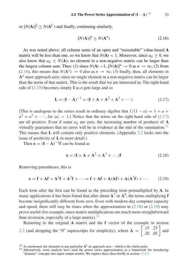
L = (I − A)−1 = (I + A + A2 + A3 + · · · ) (2.17)
[This is analogous to the series result in ordinary algebra that 1/(1 − a) = 1 + a +a2 + a3 + · · · , for |a| < 1.] Notice that the terms on the right-hand side of (2.17)are all positive. Even if some aij are zero, the increasing number of products of Avirtually guarantees that no zeros will be in evidence at the end of the summation.12
This means that L will contain only positive elements. (Appendix 2.2 looks into theissue of positivity of L in more detail.)
Then x = (I − A)−1f can be found as
x = (I + A + A2 + A3 + · · · )f (2.18)
Removing parentheses, this is
x = f + Af + A2f + A3f + · · · = f + Af + A(Af) + A(A2f) + · · · (2.19)
Each term after the first can be found as the preceding term premultiplied by A. Inmany applications it has been found that after about A7 or A8, the terms multiplying fbecome insignificantly different from zero. Even with modern-day computer capacityand speed, there still may be times when the approximation in (2.18) or (2.19) mayprove useful (for example, since matrix multiplications are much more straightforwardthan inversion, especially of a large matrix).13
Returning to the original A matrix and the f vector of the example in section
2.3 (and dropping the “0” superscripts for simplicity), where A =[
.15 .25
.20 .05
]and
12 As mentioned, the elements in any particular Ak do approach zero – which is the whole point.13 Alternatively, some analysts have used the power series approximation as a framework for introducing
“dynamic” concepts into input–output models. We explore these ideas briefly in section 13.4.7.
34 Foundations of Input–Output Analysis
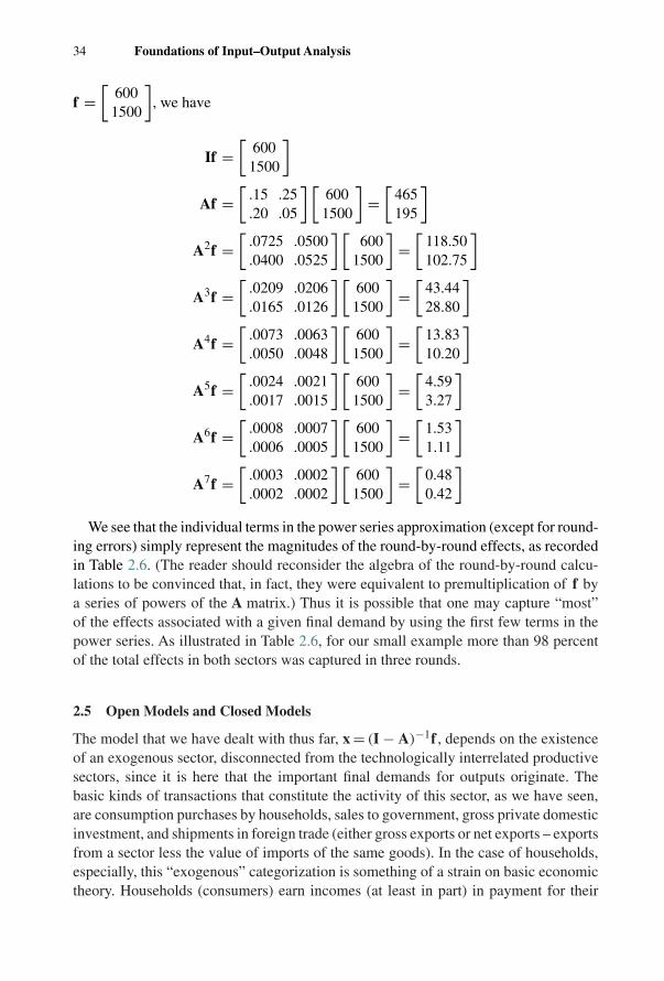
f =[
6001500
], we have
If =[
6001500
]Af =
[.15 .25.20 .05
] [600
1500
]=[
465195
]A2f =
[.0725 .0500.0400 .0525
] [600
1500
]=[
118.50102.75
]A3f =
[.0209 .0206.0165 .0126
] [600
1500
]=[
43.4428.80
]A4f =
[.0073 .0063.0050 .0048
] [600
1500
]=[
13.8310.20
]A5f =
[.0024 .0021.0017 .0015
] [600
1500
]=[
4.593.27
]A6f =
[.0008 .0007.0006 .0005
] [600
1500
]=[
1.531.11
]A7f =
[.0003 .0002.0002 .0002
] [600
1500
]=[
0.480.42
]We see that the individual terms in the power series approximation (except for round-
ing errors) simply represent the magnitudes of the round-by-round effects, as recordedin Table 2.6. (The reader should reconsider the algebra of the round-by-round calcu-lations to be convinced that, in fact, they were equivalent to premultiplication of f bya series of powers of the A matrix.) Thus it is possible that one may capture “most”of the effects associated with a given final demand by using the first few terms in thepower series. As illustrated in Table 2.6, for our small example more than 98 percentof the total effects in both sectors was captured in three rounds.
2.5 Open Models and Closed Models
The model that we have dealt with thus far, x = (I − A)−1f , depends on the existenceof an exogenous sector, disconnected from the technologically interrelated productivesectors, since it is here that the important final demands for outputs originate. Thebasic kinds of transactions that constitute the activity of this sector, as we have seen,are consumption purchases by households, sales to government, gross private domesticinvestment, and shipments in foreign trade (either gross exports or net exports – exportsfrom a sector less the value of imports of the same goods). In the case of households,especially, this “exogenous” categorization is something of a strain on basic economictheory. Households (consumers) earn incomes (at least in part) in payment for their
2.5 Open Models and Closed Models 35
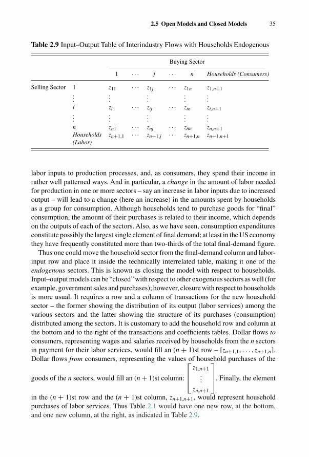
Table 2.9 Input–Output Table of Interindustry Flows with Households Endogenous
Buying Sector
1 · · · j · · · n Households (Consumers)
Selling Sector 1 z11 · · · z1j · · · z1n z1,n+1...
......
......
i zi1 · · · zij · · · zin zi,n+1...
......
......
n zn1 · · · znj · · · znn zn,n+1Households zn+1,1 · · · zn+1,j · · · zn+1,n zn+1,n+1(Labor)
labor inputs to production processes, and, as consumers, they spend their income inrather well patterned ways. And in particular, a change in the amount of labor neededfor production in one or more sectors – say an increase in labor inputs due to increasedoutput – will lead to a change (here an increase) in the amounts spent by householdsas a group for consumption. Although households tend to purchase goods for “final”consumption, the amount of their purchases is related to their income, which dependson the outputs of each of the sectors. Also, as we have seen, consumption expendituresconstitute possibly the largest single element of final demand; at least in the US economythey have frequently constituted more than two-thirds of the total final-demand figure.
Thus one could move the household sector from the final-demand column and labor-input row and place it inside the technically interrelated table, making it one of theendogenous sectors. This is known as closing the model with respect to households.Input–output models can be “closed” with respect to other exogenous sectors as well (forexample, government sales and purchases); however, closure with respect to householdsis more usual. It requires a row and a column of transactions for the new householdsector – the former showing the distribution of its output (labor services) among thevarious sectors and the latter showing the structure of its purchases (consumption)distributed among the sectors. It is customary to add the household row and column atthe bottom and to the right of the transactions and coefficients tables. Dollar flows toconsumers, representing wages and salaries received by households from the n sectorsin payment for their labor services, would fill an (n + 1)st row – [zn+1,1, . . . , zn+1,n].Dollar flows from consumers, representing the values of household purchases of the
goods of the n sectors, would fill an (n + 1)st column:
⎡⎢⎣ z1,n+1...
zn,n+1
⎤⎥⎦. Finally, the element
in the (n + 1)st row and the (n + 1)st column, zn+1,n+1, would represent householdpurchases of labor services. Thus Table 2.1 would have one new row, at the bottom,and one new column, at the right, as indicated in Table 2.9.
36 Foundations of Input–Output Analysis
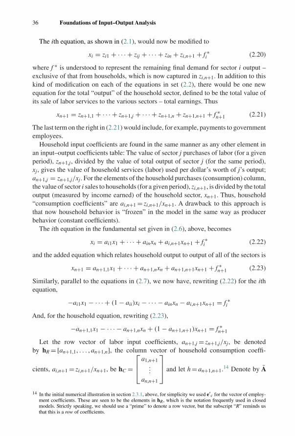
The ith equation, as shown in (2.1), would now be modified to
xi = zi1 + · · · + zij + · · · + zin + zi,n+1 + f ∗i (2.20)
where f ∗ is understood to represent the remaining final demand for sector i output –exclusive of that from households, which is now captured in zi,n+1. In addition to thiskind of modification on each of the equations in set (2.2), there would be one newequation for the total “output” of the household sector, defined to be the total value ofits sale of labor services to the various sectors – total earnings. Thus
xn+1 = zn+1,1 + · · · + zn+1,j + · · · + zn+1,n + zn+1,n+1 + f ∗n+1 (2.21)
The last term on the right in (2.21) would include, for example, payments to governmentemployees.
Household input coefficients are found in the same manner as any other element inan input–output coefficients table: The value of sector j purchases of labor (for a givenperiod), zn+1,j, divided by the value of total output of sector j (for the same period),xj, gives the value of household services (labor) used per dollar’s worth of j’s output;an+1,j = zn+1,j/xj. For the elements of the household purchases (consumption) column,the value of sector i sales to households (for a given period), zi,n+1, is divided by the totaloutput (measured by income earned) of the household sector, xn+1. Thus, household“consumption coefficients” are ai,n+1 = zi,n+1/xn+1. A drawback to this approach isthat now household behavior is “frozen” in the model in the same way as producerbehavior (constant coefficients).
The ith equation in the fundamental set given in (2.6), above, becomes
xi = ai1x1 + · · · + ainxn + ai,n+1xn+1 + f ∗i (2.22)
and the added equation which relates household output to output of all of the sectors is
xn+1 = an+1,1x1 + · · · + an+1,nxn + an+1,n+1xn+1 + f ∗n+1 (2.23)
Similarly, parallel to the equations in (2.7), we now have, rewriting (2.22) for the ithequation,
−ai1x1 − · · · + (1 − aii)xi − · · · − ainxn − ai,n+1xn+1 = f ∗i
And, for the household equation, rewriting (2.23),
−an+1,1x1 − · · · − an+1,nxn + (1 − an+1,n+1)xn+1 = f ∗n+1
Let the row vector of labor input coefficients, an+1,j = zn+1,j/xj, be denotedby hR = [an+1,1, . . . , an+1,n], the column vector of household consumption coeffi-
cients, ai,n+1 = zi,n+1/xn+1, be hC =⎡⎢⎣ a1,n+1
...an,n+1
⎤⎥⎦ and let h = an+1,n+1.14 Denote by A
14 In the initial numerical illustration in section 2.3.1, above, for simplicity we used e′c for the vector of employ-
ment coefficients. These are seen to be the elements in hR, which is the notation frequently used in closedmodels. Strictly speaking, we should use a “prime” to denote a row vector, but the subscript “R” reminds usthat this is a row of coefficients.
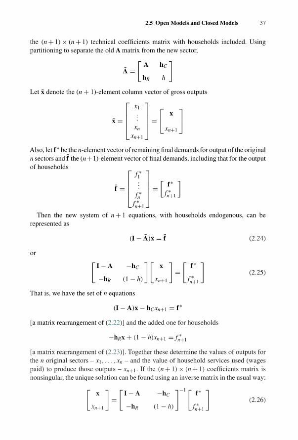
2.5 Open Models and Closed Models 37
the (n + 1) × (n + 1) technical coefficients matrix with households included. Usingpartitioning to separate the old A matrix from the new sector,
A =[
A hC
hR h
]
Let x denote the (n + 1)-element column vector of gross outputs
x =
⎡⎢⎢⎢⎣x1...
xn
xn+1
⎤⎥⎥⎥⎦ =⎡⎣ x
xn+1
⎤⎦Also, let f∗ be the n-element vector of remaining final demands for output of the originaln sectors and f the (n+1)-element vector of final demands, including that for the outputof households
f =
⎡⎢⎢⎢⎣f ∗1...
f ∗n
f ∗n+1
⎤⎥⎥⎥⎦ =[
f∗f ∗n+1
]
Then the new system of n + 1 equations, with households endogenous, can berepresented as
(I − A)x = f (2.24)
or [I − A −hC
−hR (1 − h)
][x
xn+1
]=[
f∗
f ∗n+1
](2.25)
That is, we have the set of n equations
(I − A)x − hCxn+1 = f∗
[a matrix rearrangement of (2.22)] and the added one for households
−hRx + (1 − h)xn+1 = f ∗n+1
[a matrix rearrangement of (2.23)]. Together these determine the values of outputs forthe n original sectors – x1, . . . , xn – and the value of household services used (wagespaid) to produce those outputs – xn+1. If the (n + 1) × (n + 1) coefficients matrix isnonsingular, the unique solution can be found using an inverse matrix in the usual way:[
x
xn+1
]=[
I − A −hC
−hR (1 − h)
]−1 [ f∗
f ∗n+1
](2.26)
38 Foundations of Input–Output Analysis
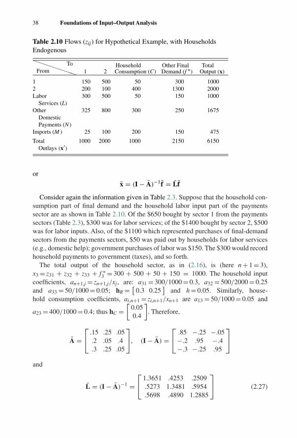
Table 2.10 Flows (zij) for Hypothetical Example, with HouseholdsEndogenous
�������FromTo Household Other Final Total
1 2 Consumption (C) Demand (f ∗) Output (x)
1 150 500 50 300 10002 200 100 400 1300 2000Labor
Services (L)
300 500 50 150 1000
OtherDomesticPayments (N )
325 800 300 250 1675
Imports (M ) 25 100 200 150 475
TotalOutlays (x′)
1000 2000 1000 2150 6150
or
x = (I − A)−1f = Lf
Consider again the information given in Table 2.3. Suppose that the household con-sumption part of final demand and the household labor input part of the paymentssector are as shown in Table 2.10. Of the $650 bought by sector 1 from the paymentssectors (Table 2.3), $300 was for labor services; of the $1400 bought by sector 2, $500was for labor inputs. Also, of the $1100 which represented purchases of final-demandsectors from the payments sectors, $50 was paid out by households for labor services(e.g., domestic help); government purchases of labor was $150. The $300 would recordhousehold payments to government (taxes), and so forth.
The total output of the household sector, as in (2.16), is (here n + 1 = 3),x3 = z31 + z32 + z33 + f ∗
3 = 300 + 500 + 50 + 150 = 1000. The household inputcoefficients, an+1,j = zn+1,j/xj, are: a31 = 300/1000 = 0.3, a32 = 500/2000 = 0.25and a33 = 50/1000 = 0.05; hR = [
0.3 0.25]
and h = 0.05. Similarly, house-hold consumption coefficients, ai,n+1 = zi,n+1/xn+1 are a13 = 50/1000 = 0.05 and
a23 = 400/1000 = 0.4; thus hC =[
0.050.4
]. Therefore,
A =⎡⎣ .15 .25 .05
.2 .05 .4
.3 .25 .05
⎤⎦, (I − A) =⎡⎣ .85 −.25 −.05
−.2 .95 −.4−.3 −.25 .95
⎤⎦and
L = (I − A)−1 =⎡⎣ 1.3651 .4253 .2509
.5273 1.3481 .5954
.5698 .4890 1.2885
⎤⎦ (2.27)
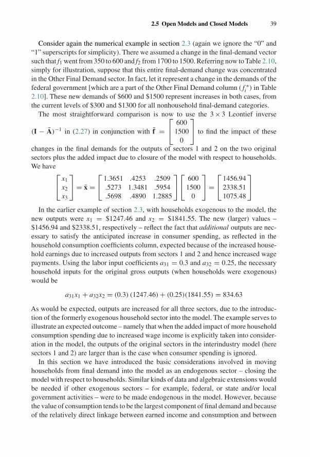
2.5 Open Models and Closed Models 39
Consider again the numerical example in section 2.3 (again we ignore the “0” and“1” superscripts for simplicity). There we assumed a change in the final-demand vectorsuch that f1 went from 350 to 600 and f2 from 1700 to 1500. Referring now to Table 2.10,simply for illustration, suppose that this entire final-demand change was concentratedin the Other Final Demand sector. In fact, let it represent a change in the demands of thefederal government [which are a part of the Other Final Demand column ( f ∗
i ) in Table2.10]. These new demands of $600 and $1500 represent increases in both cases, fromthe current levels of $300 and $1300 for all nonhousehold final-demand categories.
The most straightforward comparison is now to use the 3 × 3 Leontief inverse
(I − A)−1 in (2.27) in conjunction with f =⎡⎣ 600
15000
⎤⎦ to find the impact of these
changes in the final demands for the outputs of sectors 1 and 2 on the two originalsectors plus the added impact due to closure of the model with respect to households.We have⎡⎣ x1
x2
x3
⎤⎦ = x =⎡⎣ 1.3651 .4253 .2509
.5273 1.3481 .5954
.5698 .4890 1.2885
⎤⎦⎡⎣ 6001500
0
⎤⎦ =⎡⎣ 1456.94
2338.511075.48
⎤⎦In the earlier example of section 2.3, with households exogenous to the model, the
new outputs were x1 = $1247.46 and x2 = $1841.55. The new (larger) values –$1456.94 and $2338.51, respectively – reflect the fact that additional outputs are nec-essary to satisfy the anticipated increase in consumer spending, as reflected in thehousehold consumption coefficients column, expected because of the increased house-hold earnings due to increased outputs from sectors 1 and 2 and hence increased wagepayments. Using the labor input coefficients a31 = 0.3 and a32 = 0.25, the necessaryhousehold inputs for the original gross outputs (when households were exogenous)would be
a31x1 + a32x2 = (0.3) (1247.46) + (0.25)(1841.55) = 834.63
As would be expected, outputs are increased for all three sectors, due to the introduc-tion of the formerly exogenous household sector into the model. The example serves toillustrate an expected outcome – namely that when the added impact of more householdconsumption spending due to increased wage income is explicitly taken into consider-ation in the model, the outputs of the original sectors in the interindustry model (heresectors 1 and 2) are larger than is the case when consumer spending is ignored.
In this section we have introduced the basic considerations involved in movinghouseholds from final demand into the model as an endogenous sector – closing themodel with respect to households. Similar kinds of data and algebraic extensions wouldbe needed if other exogenous sectors – for example, federal, or state and/or localgovernment activities – were to be made endogenous in the model. However, becausethe value of consumption tends to be the largest component of final demand and becauseof the relatively direct linkage between earned income and consumption and between
40 Foundations of Input–Output Analysis
consumption and output, the household sector is the one final-demand sector that ismost often moved inside the model.
In practice, however, the issue is far more subtle, and the procedure is more com-plicated than might be suggested by the discussion in this section. All of the previousreservations about the aij apply here as well, if not with greater force. For each addi-tional dollar of received earnings, households are assumed to spend 5 cents on the outputof sector 1, 40 cents on the output of sector 2, and so on. Those coefficients, whichreflect average behavior during the observation period when household income was$1000 (a13 = 50/1000 and a23 = 400/1000), are assumed to hold for the additional, ormarginal, amounts of household earnings associated with the new outputs of sectors 1and 2. One approach, particularly at the regional level, is to divide consumers into twogroups: established residents, for whom the new income associated with new productionwould represent an addition to current earnings, and new residents (in-migrants), whomay have moved in search of employment and for whom the new income representstotal earnings. For the former group, a set of marginal consumption coefficients mightbe appropriate, while for the latter group average consumption coefficients would berelevant.
In addition, spending patterns of consumers, especially out of additions to (or reduc-tions in) disposable income, will depend on the income category in which a particularconsumer is located. An addition of $100 to the spendable income of a worker earning$20,000 per year is likely to be spent differently than an additional $100 in the hands ofan engineer with an annual income of $150,000, and both will no doubt differ from theway in which the $100 would be spent by a previously unemployed person. In effect,this is simply noting that inputs to the household sector (consumption) per dollar ofoutput (household income) will not be independent of the level of that output. Yet suchindependence is assumed in the way that the direct input coefficients are used in aninput–output model; each sector’s production function (column of direct input coeffi-cients) is assumed to represent inputs per dollar’s worth of output, regardless of theamount (level) of that output.
Another approach, then, is to disaggregate “the” household sector into several sectors,distinguished by total income. For example, $0–$10,000, $10,001–$20,000, $20,001–$30,000; and so on. Consumption coefficients, by sector, could then be derived foreach income class. We will return to this issue in a regional context in Chapter 3 and inChapter 10 when examining social accounting matrices. A very thorough discussion ofan approach for incorporating a disaggregated household sector into the endogenouspart of an input–output model, using a good deal of matrix algebra, can be found inMiyazawa (1976). We explore that model in more detail in Chapter 6.
Further disaggregations of the household sector have been proposed and incorporatedin input–output analysis. These frameworks fall into the category of what are knownas “extended” input–output models. (For a concise overview see Batey, Madden andWeeks, 1987 or Batey and Weeks, 1989.) The idea is to separate income payments toand consumption patterns of different household groups – for example, established vs.new residents (noted above) and currently employed vs. unemployed.
2.6 The Price Model 41
One could imagine a process of moving, one by one, each of the remaining sectorsfrom the final-demand vector into the interindustry coefficients matrix, constructingrows of input coefficients and columns of purchase coefficients until there were noexogenous sectors at all. This is termed a completely closed model. However, theeconomic logic behind fixed coefficients in the case, say, of a government sector isless easy to accept than for the productive sectors, and completely closed models areseldom implemented in practice.15
2.6 The Price Model
2.6.1 OverviewLeontief originally developed the input–output model in physical units (bushels ofwheat, yards of cloth, man-years of labor, etc.).16 In particular, he assumed that directinput coefficients, A, are based on physical quantities of inputs divided by physicalquantities of output. These data were then converted to a table of (base year) transactionsin value terms by using (base year) unit prices – for a bushel of wheat, a yard of clothand a man-year of labor. He writes (Leontief, 1986, pp. 22–23):
All figures [in the value transactions table]…can also be interpreted as representing physical quantitiesof the goods or services to which they refer. This only requires that the physical unit in which theentries…are measured be redefined as being equal to that amount of output of that particular sectorthat can be purchased for $1 at [base year] prices… In practice the structural matrices are usuallycomputed from input-output tables described in value terms…In any case, the input coefficients [A] –for analytical purposes…must be interpreted as ratios of two quantities measured in physical units[emphasis added].
As already noted, input–output data are usually assembled and input–output studies aregenerally carried out in monetary (value) units.
However, with the emergence of energy and environmental concerns, mixed-unitsmodels have been developed, where economic transactions are recorded in monetaryterms and ecological and/or energy transactions are recorded in physical terms (tons,BTUs, joules, etc.).17 Another line of inquiry has led to input–output tables in commonphysical units (e.g., all transactions and outputs measured in tons). Stahmer (2000)gives an overview of this kind of work, including tables for Germany for 1990 inboth monetary and physical units – sometimes designated MIOTs and PIOTs, respec-tively. (There are problems in trying to measure outputs of services in physical units.)18
We explore a small illustration in section 2.6.8, below, using an aggregation of theGerman data.
15 The original work done by Leontief, however, was in the framework of a completely closed model of the UnitedStates for 1919. See Leontief (1951b).
16 See, for example, Leontief (1951a, 1951b, 1986), Leontief et al. (1953).17 These issues are explored further in Chapters 9 and 10.18 Stahmer (2000) also introduces the notion of data measured in time units, leading to TIOTs.
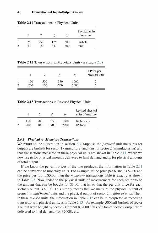
42 Foundations of Input–Output Analysis
Table 2.11 Transactions in Physical Units
Physical units1 2 di qi of measure
1 75 250 175 500 bushels2 40 20 340 400 tons
Table 2.12 Transactions in Monetary Units (see Table 2.3)
$ Price per1 2 fi xi physical unit
1 150 500 350 1000 22 200 100 1700 2000 5
Table 2.13 Transactions in Revised Physical Units
Revised physical1 2 di qi units of measure
1 150 500 350 1000 1/2 bushels2 200 100 1700 2000 1/5 tons
2.6.2 Physical vs. Monetary TransactionsWe return to the illustration in section 2.3. Suppose the physical unit measures foroutputs are bushels for sector 1 (agriculture) and tons for sector 2 (manufacturing) andthat transactions measured in these physical units are shown in Table 2.11, where wenow use di for physical amounts delivered to final demand and qi for physical amountsof total output.
If we know the per-unit prices of the two products, the information in Table 2.11can be converted to monetary units. For example, if the price per bushel is $2.00 andthe price per ton is $5.00, then the monetary transactions table is exactly as shownin Table 2.3. Now, redefine the physical units of measurement for each sector to bethe amount that can be bought for $1.00; that is, so that the per-unit price for eachsector’s output is $1.00. This simply means that we measure the physical output ofsector 1 in half bushel units and the physical output of sector 2 in fifths of a ton. Then,in these revised units, the information in Table 2.12 can be reinterpreted as recordingtransactions in physical units, as in Table 2.13 – for example, 500 half-bushels of sector1 output were bought by sector 2 (for $500), 2000 fifths of a ton of sector 2 output weredelivered to final demand (for $2000), etc.
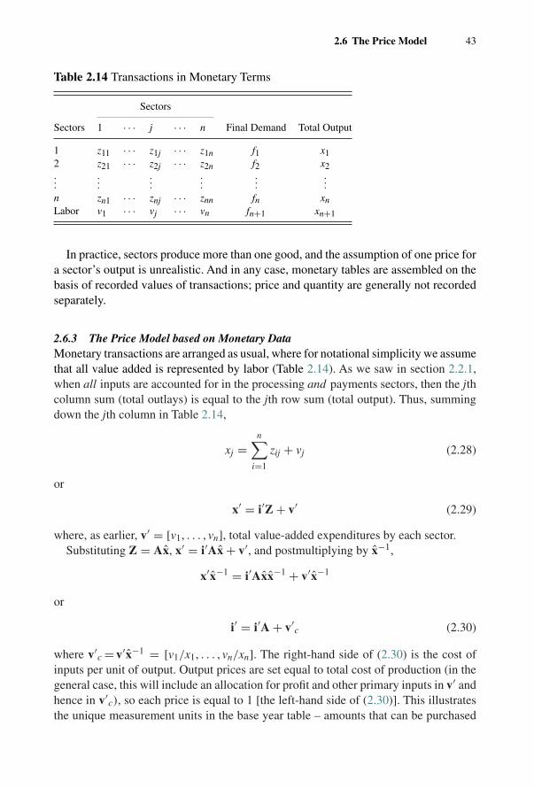
2.6 The Price Model 43
Table 2.14 Transactions in Monetary Terms
Sectors
Sectors 1 · · · j · · · n Final Demand Total Output
1 z11 · · · z1j · · · z1n f1 x12 z21 · · · z2j · · · z2n f2 x2...
......
......
...n zn1 · · · znj · · · znn fn xnLabor v1 · · · vj · · · vn fn+1 xn+1
In practice, sectors produce more than one good, and the assumption of one price fora sector’s output is unrealistic. And in any case, monetary tables are assembled on thebasis of recorded values of transactions; price and quantity are generally not recordedseparately.
2.6.3 The Price Model based on Monetary DataMonetary transactions are arranged as usual, where for notational simplicity we assumethat all value added is represented by labor (Table 2.14). As we saw in section 2.2.1,when all inputs are accounted for in the processing and payments sectors, then the jthcolumn sum (total outlays) is equal to the jth row sum (total output). Thus, summingdown the jth column in Table 2.14,
xj =n∑
i=1
zij + vj (2.28)
or
x′ = i′Z + v′ (2.29)
where, as earlier, v′ = [v1, . . . , vn], total value-added expenditures by each sector.Substituting Z = Ax, x′ = i′Ax + v′, and postmultiplying by x−1,
x′x−1 = i′Axx−1 + v′x−1
or
i′ = i′A + v′c (2.30)
where v′c = v′x−1 = [v1/x1, . . . , vn/xn]. The right-hand side of (2.30) is the cost of
inputs per unit of output. Output prices are set equal to total cost of production (in thegeneral case, this will include an allocation for profit and other primary inputs in v′ andhence in v′
c), so each price is equal to 1 [the left-hand side of (2.30)]. This illustratesthe unique measurement units in the base year table – amounts that can be purchased
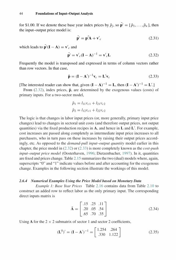
44 Foundations of Input–Output Analysis
for $1.00. If we denote these base year index prices by pj, so p′ = [ p1, . . . , pn ], thenthe input–output price model is:
p′ = ˜p′A + v′c (2.31)
which leads to p′(I − A) = v′c and
p′ = v′c(I − A)−1 = v′
cL (2.32)
Frequently the model is transposed and expressed in terms of column vectors ratherthan row vectors. In that case,
p = (I − A′)−1vc = L′vc (2.33)
[The interested reader can show that, given (I − A)−1 = L, then (I − A′)−1 = L′.]From (2.32), index prices, p, are determined by the exogenous values (costs) of
primary inputs. For a two-sector model,
p1 = l11vc1 + l21vc2
p2 = l12vc1 + l22vc2
The logic is that changes in labor input prices (or, more generally, primary input pricechanges) lead to changes in sectoral unit costs (and therefore output prices, not outputquantities) via the fixed production recipes in A, and hence in L and L′. For example,cost increases are passed along completely as intermediate input price increases to allpurchasers, who in turn pass on these increases by raising their output prices accord-ingly, etc. As opposed to the demand-pull input–output quantity model earlier in thischapter, the price model in (2.32) or (2.33) is more completely known as the cost-pushinput–output price model (Oosterhaven, 1996; Dietzenbacher, 1997). In it, quantitiesare fixed and prices change. Table 2.15 summarizes the two (dual) models where, again,superscripts “0” and “1” indicate values before and after accounting for the exogenouschange. Examples in the following section illustrate the workings of this model.
2.6.4 Numerical Examples Using the Price Model based on Monetary DataExample 1: Base Year Prices Table 2.16 contains data from Table 2.10 to
construct an added row to reflect labor as the only primary input. The correspondingdirect inputs matrix is
A =⎡⎣ .15 .25 .11
.20 .05 .54
.65 .70 .35
⎤⎦ (2.34)
Using A for the 2 × 2 submatrix of sector 1 and sector 2 coefficients,
(L0)′ = (I − A′)−1 =[
1.254 .264.330 1.122
](2.35)
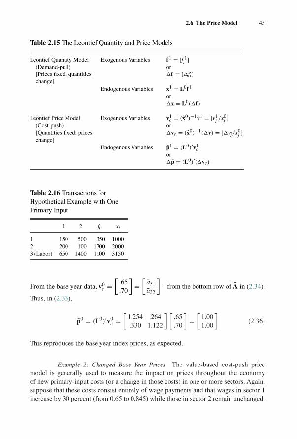
2.6 The Price Model 45
Table 2.15 The Leontief Quantity and Price Models
Leontief Quantity Model(Demand-pull)[Prices fixed; quantitieschange]
Exogenous Variables f1 = [f 1i ]
or�f = [�fi]
Endogenous Variables x1 = L0f1
or�x = L0(�f)
Leontief Price Model(Cost-push)[Quantities fixed; priceschange]
Exogenous Variables v1c = (x0)−1v1 = [v1
j /x0j ]
or�vc = (x0)−1(�v) = [�vj/x0
j ]
Endogenous Variables p1 = (L0)′v1c
or�p = (L0)′(�vc)
Table 2.16 Transactions forHypothetical Example with OnePrimary Input
1 2 fi xi
1 150 500 350 10002 200 100 1700 20003 (Labor) 650 1400 1100 3150
From the base year data, v0c =
[.65.70
]=[
a31
a32
]– from the bottom row of A in (2.34).
Thus, in (2.33),
p0 = (L0)′v0c =
[1.254 .264.330 1.122
] [.65.70
]=[
1.001.00
](2.36)
This reproduces the base year index prices, as expected.
Example 2: Changed Base Year Prices The value-based cost-push pricemodel is generally used to measure the impact on prices throughout the economyof new primary-input costs (or a change in those costs) in one or more sectors. Again,suppose that these costs consist entirely of wage payments and that wages in sector 1increase by 30 percent (from 0.65 to 0.845) while those in sector 2 remain unchanged.
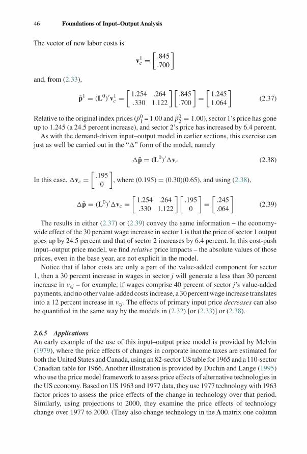
46 Foundations of Input–Output Analysis
The vector of new labor costs is
v1c =
[.845.700
]and, from (2.33),
p1 = (L0)′v1c =
[1.254 .264.330 1.122
] [.845.700
]=[
1.2451.064
](2.37)
Relative to the original index prices (p01 = 1.00 and p0
2 = 1.00), sector 1’s price has goneup to 1.245 (a 24.5 percent increase), and sector 2’s price has increased by 6.4 percent.
As with the demand-driven input–output model in earlier sections, this exercise canjust as well be carried out in the “�” form of the model, namely
�p = (L0)′�vc (2.38)
In this case, �vc =[
.1950
], where (0.195) = (0.30)(0.65), and using (2.38),
�p = (L0)′�vc =[
1.254 .264.330 1.122
] [.195
0
]=[
.245
.064
](2.39)
The results in either (2.37) or (2.39) convey the same information – the economy-wide effect of the 30 percent wage increase in sector 1 is that the price of sector 1 outputgoes up by 24.5 percent and that of sector 2 increases by 6.4 percent. In this cost-pushinput–output price model, we find relative price impacts – the absolute values of thoseprices, even in the base year, are not explicit in the model.
Notice that if labor costs are only a part of the value-added component for sector1, then a 30 percent increase in wages in sector j will generate a less than 30 percentincrease in vcj – for example, if wages comprise 40 percent of sector j’s value-addedpayments, and no other value-added costs increase, a 30 percent wage increase translatesinto a 12 percent increase in vcj. The effects of primary input price decreases can alsobe quantified in the same way by the models in (2.32) [or (2.33)] or (2.38).
2.6.5 ApplicationsAn early example of the use of this input–output price model is provided by Melvin(1979), where the price effects of changes in corporate income taxes are estimated forboth the United States and Canada, using an 82-sector US table for 1965 and a 110-sectorCanadian table for 1966. Another illustration is provided by Duchin and Lange (1995)who use the price model framework to assess price effects of alternative technologies inthe US economy. Based on US 1963 and 1977 data, they use 1977 technology with 1963factor prices to assess the price effects of the change in technology over that period.Similarly, using projections to 2000, they examine the price effects of technologychange over 1977 to 2000. (They also change technology in the A matrix one column
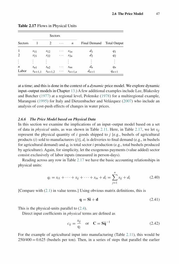
2.6 The Price Model 47
Table 2.17 Flows in Physical Units
Sectors
Sectors 1 2 · · · n Final Demand Total Output
1 s11 s12 · · · s1n d1 q12 s21 s22 · · · s2n d2 q2...
......
......
...n sn1 sn2 · · · snn dn qnLabor sn+1,1 sn+1,2 · · · sn+1,n dn+1 qn+1
at a time; and this is done in the context of a dynamic price model. We explore dynamicinput–output models in Chapter 13.) A few additional examples include Lee, Blakesleyand Butcher (1977) at a regional level, Polenske (1978) for a multiregional example,Marangoni (1995) for Italy and Dietzenbacher and Velázquez (2007) who include ananalysis of cost-push effects of changes in water prices.
2.6.6 The Price Model based on Physical DataIn this section we examine the implications of an input–output model based on a setof data in physical units, as was shown in Table 2.11. Here, in Table 2.17, we let sij
represent the physical quantity of i goods shipped to j [e.g., bushels of agriculturalproducts (i) sold to manufacturers (j)], di is deliveries to final demand (e.g., in bushelsfor agricultural demand) and qi is total sector i production (e.g., total bushels producedby agriculture). Again, for simplicity, let the exogenous payments (value added) sectorconsist exclusively of labor inputs (measured in person-days).
Reading across any row in Table 2.17 we have the basic accounting relationships inphysical units:
qi = si1 + · · · + sij + · · · + sin + di =n∑
j=1
sij + di (2.40)
[Compare with (2.1) in value terms.] Using obvious matrix definitions, this is
q = Si + d (2.41)
This is the physical-units parallel to (2.4).Direct input coefficients in physical terms are defined as
cij = sij
qjor C = Sq−1 (2.42)
For the example of agricultural input into manufacturing (Table 2.11), this would be250/400 = 0.625 (bushels per ton). Then, in a series of steps that parallel the earlier
48 Foundations of Input–Output Analysis
development of the value-based model in section 2.2, substitution into (2.41) gives
q = Cqi + d = Cq + d
from which
q = (I − C)−1d (2.43)
This is the physical-units model parallel to (2.11).
Introduction of Prices Suppose also that we know the per-unit price for eachsector’s output, pi, and the labor cost per person-hour, pn+1. Then, as Leontief observesin the quotation above, we can easily convert the basic data to the value units fromearlier in this chapter:
xi = piqi (2.44)
zij = pisij (2.45)
fi = pidi (2.46)
Multiplying (2.40) on both sides by pi gives
xi = piqi =n∑
j=1
pisij + pidi =n∑
j=1
zij + fi (2.47)
or x = Zi + f . These are, of course, the original accounting relationships in (2.1) and(2.3) in value terms.
In section 2.6.1, the representation of total outputs in terms of column sums of Table
2.14 was given in monetary terms in (2.28), namely xj =n∑
i=1zij + vj. Column sums
are not meaningful in Table 2.17 since elements in each row are measured in differentunits. The objective now is to introduce the results from (2.44) and (2.45) into (2.28).Assume, for now, that the wage rate is pn+1(dollars per person-hour) across all sectors.Then zn+1,j = pn+1sn+1,j = vj; this represents sector j’s total expenditure on labor – theprice, pn+1, times total person-hours of labor, sn+1,j. Then (2.28) becomes
pjqj =n∑
i=1
pisij + pn+1sn+1,j (2.48)
Dividing by qj (which we assume is not zero),
pj =n∑
i=1
pisij/qj + pn+1sn+1,j/qj =n∑
i=1
picij + pn+1cn+1,j (2.49)
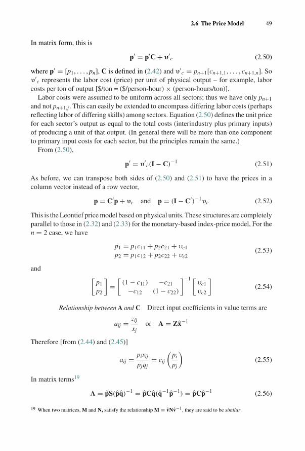
2.6 The Price Model 49
In matrix form, this is
p′ = p′C + υ′c (2.50)
where p′ = [p1, . . . , pn], C is defined in (2.42) and υ′c = pn+1[cn+1,1, . . . , cn+1,n]. So
υ′c represents the labor cost (price) per unit of physical output – for example, labor
costs per ton of output [$/ton = ($/person-hour) × (person-hours/ton)].Labor costs were assumed to be uniform across all sectors; thus we have only pn+1
and not pn+1,j. This can easily be extended to encompass differing labor costs (perhapsreflecting labor of differing skills) among sectors. Equation (2.50) defines the unit pricefor each sector’s output as equal to the total costs (interindustry plus primary inputs)of producing a unit of that output. (In general there will be more than one componentto primary input costs for each sector, but the principles remain the same.)
From (2.50),
p′ = υ′c(I − C)−1 (2.51)
As before, we can transpose both sides of (2.50) and (2.51) to have the prices in acolumn vector instead of a row vector,
p = C′p + υc and p = (I − C′)−1υc (2.52)
This is the Leontief price model based on physical units. These structures are completelyparallel to those in (2.32) and (2.33) for the monetary-based index-price model, For then = 2 case, we have
p1 = p1c11 + p2c21 + υc1
p2 = p1c12 + p2c22 + υc2(2.53)
and [p1
p2
]=[
(1 − c11) −c21
−c12 (1 − c22)
]−1 [υc1
υc2
](2.54)
Relationship between A and C Direct input coefficients in value terms are
aij = zij
xjor A = Zx−1
Therefore [from (2.44) and (2.45)]
aij = pisij
pjqj= cij
(pi
pj
)(2.55)
In matrix terms19
A = pS(pq)−1 = pCq(q−1p−1) = pCp−1 (2.56)
19 When two matrices, M and N, satisfy the relationship M = vNv−1, they are said to be similar.
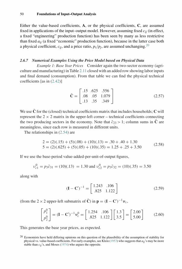
50 Foundations of Input–Output Analysis
Either the value-based coefficients, A, or the physical coefficients, C, are assumedfixed in applications of the input–output model. However, assuming fixed cij (in effect,a fixed “engineering” production function) has been seen by many as less restrictivethan fixed aij (a fixed “economic” production function), because in the latter case botha physical coefficient, cij, and a price ratio, pi/pj, are assumed unchanging.20
2.6.7 Numerical Examples Using the Price Model based on Physical DataExample 1: Base Year Prices Consider again the two-sector economy (agri-
culture and manufacturing) in Table 2.11 closed with an added row showing labor inputsand final demand (consumption). From that table we can find the physical technicalcoefficients [as in (2.42)]
C =⎡⎣ .15 .625 .556
.08 .05 1.079
.13 .35 .349
⎤⎦ (2.57)
We use C for the (closed) technical coefficients matrix that includes households; C willrepresent the 2 × 2 matrix in the upper-left corner – technical coefficients connectingthe two producing sectors in the economy. Note that c23 > 1; column sums in C aremeaningless, since each row is measured in different units.
The relationships in (2.54) are
2 = (2)(.15) + (5)(.08) + (10)(.13) = .30 + .40 + 1.305 = (2)(.625) + (5)(.05) + (10)(.35) = 1.25 + .25 + 3.50
(2.58)
If we use the base-period value-added-per-unit-of-output figures,
υ0c1 = p3c31 = (10)(.13) = 1.30 and υ0
c2 = p3c32 = (10)(.35) = 3.50
along with
(I − C′)−1 =[
1.243 .106.825 1.122
](2.59)
(from the 2 × 2 upper-left submatrix of C) in p = (I − C′)−1υc,[p0
1
p02
]= (I − C′)−1υ0
c =[
1.254 .106.825 1.122
] [1.33.5
]=[
2.005.00
](2.60)
This generates the base year prices, as expected.
20 Economists have held differing opinions on this question of the plausibility of the assumption of stability forphysical vs. value-based coefficients. For early examples, see Klein (1953) who suggests that aij’s may be morestable than cij’s, and Moses (1974) who argues the opposite.
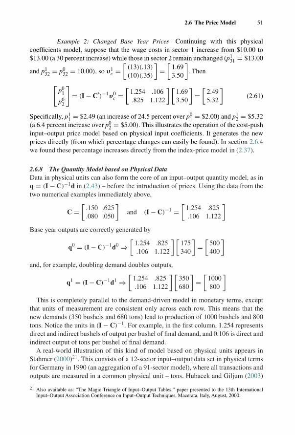
2.6 The Price Model 51
Example 2: Changed Base Year Prices Continuing with this physicalcoefficients model, suppose that the wage costs in sector 1 increase from $10.00 to$13.00 (a 30 percent increase) while those in sector 2 remain unchanged (p1
31 = $13.00
and p132 = p0
32 = 10.00), so υ1c =
[(13)(.13)
(10)(.35)
]=[
1.693.50
]. Then
[p0
1
p02
]= (I − C′)−1υ0
c =[
1.254 .106.825 1.122
] [1.693.50
]=[
2.495.32
](2.61)
Specifically, p11 = $2.49 (an increase of 24.5 percent over p0
1 = $2.00) and p12 = $5.32
(a 6.4 percent increase over p02 = $5.00). This illustrates the operation of the cost-push
input–output price model based on physical input coefficients. It generates the newprices directly (from which percentage changes can easily be found). In section 2.6.4we found these percentage increases directly from the index-price model in (2.37).
2.6.8 The Quantity Model based on Physical DataData in physical units can also form the core of an input–output quantity model, as inq = (I − C)−1d in (2.43) – before the introduction of prices. Using the data from thetwo numerical examples immediately above,
C =[
.150 .625
.080 .050
]and (I − C)−1 =
[1.254 .825.106 1.122
]Base year outputs are correctly generated by
q0 = (I − C)−1d0 ⇒[
1.254 .825.106 1.122
] [175340
]=[
500400
]and, for example, doubling demand doubles outputs,
q1 = (I − C)−1d1 ⇒[
1.254 .825.106 1.122
] [350680
]=[
1000800
]This is completely parallel to the demand-driven model in monetary terms, except
that units of measurement are consistent only across each row. This means that thenew demands (350 bushels and 680 tons) lead to production of 1000 bushels and 800tons. Notice the units in (I − C)−1. For example, in the first column, 1.254 representsdirect and indirect bushels of output per bushel of final demand, and 0.106 is direct andindirect output of tons per bushel of final demand.
A real-world illustration of this kind of model based on physical units appears inStahmer (2000)21. This consists of a 12-sector input–output data set in physical termsfor Germany in 1990 (an aggregation of a 91-sector model), where all transactions andoutputs are measured in a common physical unit – tons. Hubacek and Giljum (2003)
21 Also available as: “The Magic Triangle of Input–Output Tables,” paper presented to the 13th InternationalInput–Output Association Conference on Input–Output Techniques, Macerata, Italy, August, 2000.
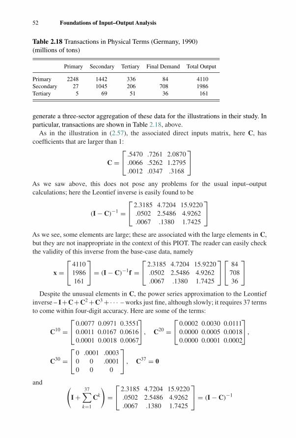
52 Foundations of Input–Output Analysis
Table 2.18 Transactions in Physical Terms (Germany, 1990)(millions of tons)
Primary Secondary Tertiary Final Demand Total Output
Primary 2248 1442 336 84 4110Secondary 27 1045 206 708 1986Tertiary 5 69 51 36 161
generate a three-sector aggregation of these data for the illustrations in their study. Inparticular, transactions are shown in Table 2.18, above.
As in the illustration in (2.57), the associated direct inputs matrix, here C, hascoefficients that are larger than 1:
C =⎡⎣ .5470 .7261 2.0870
.0066 .5262 1.2795
.0012 .0347 .3168
⎤⎦As we saw above, this does not pose any problems for the usual input–outputcalculations; here the Leontief inverse is easily found to be
(I − C)−1 =⎡⎣ 2.3185 4.7204 15.9220
.0502 2.5486 4.9262
.0067 .1380 1.7425
⎤⎦As we see, some elements are large; these are associated with the large elements in C,but they are not inappropriate in the context of this PIOT. The reader can easily checkthe validity of this inverse from the base-case data, namely
x =⎡⎣ 4110
1986161
⎤⎦ = (I − C)−1f =⎡⎣ 2.3185 4.7204 15.9220
.0502 2.5486 4.9262
.0067 .1380 1.7425
⎤⎦⎡⎣ 8470836
⎤⎦Despite the unusual elements in C, the power series approximation to the Leontief
inverse – I+C+C2 +C3 +· · · – works just fine, although slowly; it requires 37 termsto come within four-digit accuracy. Here are some of the terms:
C10 =⎡⎣ 0.0077 0.0971 0.3551
0.0011 0.0167 0.06160.0001 0.0018 0.0067
⎤⎦ , C20 =⎡⎣ 0.0002 0.0030 0.0111
0.0000 0.0005 0.00180.0000 0.0001 0.0002
⎤⎦ ,
C30 =⎡⎣ 0 .0001 .0003
0 0 .00010 0 0
⎤⎦ , C37 = 0
and (I +
37∑k=1
Ck
)=⎡⎣ 2.3185 4.7204 15.9220
.0502 2.5486 4.9262
.0067 .1380 1.7425
⎤⎦ = (I − C)−1

2.7 Summary 53
The interested reader with access to combinatorial algebra software on a computer
might check that for this illustration, with (I − C) =⎡⎣ .4530 −.7261 −2.0870
−.0066 .4738 −1.2795−.0012 −.0347 .6832
⎤⎦,
the Hawkins–Simon conditions are satisfied, meaning that all seven principal minorsof (I − C) are positive (Appendix 2.2).
2.6.9 A Basic National Income IdentityFrom (2.43), q = (I − C)−1d; from (2.51), p′ = υ′
c(I − C)−1, and postmultiplyingthis by d,
p′d = υ ′c(I − C)−1d = υ ′
cq
The total value of spending (exogenous final demand, p′d) equals the total value ofearnings (payments to exogenous primary inputs, υ ′
cq), or national income spent equalsnational income received.
2.7 Summary
We have introduced the basic structure of the input–output model in this chapter. Afterinvestigating the special features of sectoral production functions that are assumed inthe Leontief system, we examined its mathematical features. Importantly, the modelis expressed in a set of linear equations, and we have tried to indicate the connectionbetween the purely algebraic solution to the input–output equations, using the Leontiefinverse matrix, and the logical, economic content of the round-by-round view of produc-tion interrelationships in an economy. Both the algebraic details as well as the economicassumptions needed to close the model with respect to households were discussed.Some of the special problems associated with the concept of household consumptioncoefficients have been addressed in applications, especially at the regional level. Wealso introduced the Leontief price model, a logical (and mathematical) companion tothe quantity model, and we explored alternatives to both models when the underlyingdata are measured in physical rather than monetary terms. Table 2.19 summarizes thealternatives. (Information in the monetary row is in Table 2.15.)
We turn to regional input–output models in the next chapter. It is important to add theregional dimension; many if not most important policy questions are not purely nationalin scope. Rather, analysts (even at the national level) are interested in differentialregional effects of, say, a change in national government policy regarding exports.It is important to know not only the total magnitudes of the new outputs, by sector,that come about because of stimulation of exports, but also to know something oftheir geographical incidence – is a particularly depressed area helped by such exportstimulation, or does the increased output occur largely in regions that are economicallymore healthy? Extensions of the basic model to deal with issues of this sort will occupyus in Chapter 3.
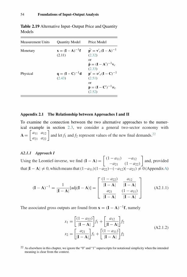
54 Foundations of Input–Output Analysis
Table 2.19 Alternative Input–Output Price and QuantityModels
Measurement Units Quantity Model Price Model
Monetary x = (I − A)−1f(2.11)
p′ = v′c(I − A)−1
(2.32)orp = (I − A′)−1vc(2.33)
Physical q = (I − C)−1d(2.43)
p′ = υ′c(I − C)−1
(2.51)orp = (I − C′)−1υc(2.52)
Appendix 2.1 The Relationship between Approaches I and II
To examine the connection between the two alternative approaches to the numer-ical example in section 2.3, we consider a general two-sector economy with
A =[
a11 a12
a21 a22
]and let f1 and f2 represent values of the new final demands.22
A2.1.1 Approach I
Using the Leontief-inverse, we find (I − A) =[
(1 − a11) −a12
−a21 (1 − a22)
]and, provided
that |I − A| �= 0, which means that (1−a11)(1−a22)−(−a12)(−a21) �= 0 (AppendixA)
(I − A)−1 = 1
|I − A| [adj(I − A)] =
⎡⎢⎢⎣(1 − a22)
|I − A|a12
|I − A|a21
|I − A|(1 − a11)
|I − A|
⎤⎥⎥⎦ (A2.1.1)
The associated gross outputs are found from x = (I − A)−1f , namely
x1 =[(1 − a22)
|I − A|]
f1 +[
a12
|I − A|]
f2
x2 =[
a21
|I − A|]
f1 +[(1 − a11)
|I − A|]
f2
(A2.1.2)
22 As elsewhere in this chapter, we ignore the “0” and “1” superscripts for notational simplicity when the intendedmeaning is clear from the context.
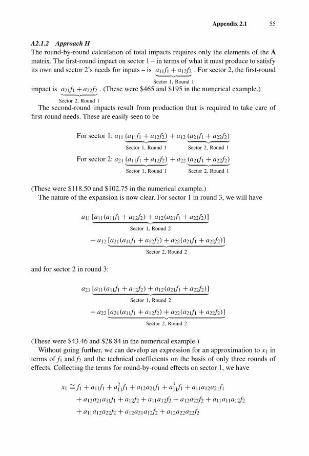
Appendix 2.1 55
A2.1.2 Approach IIThe round-by-round calculation of total impacts requires only the elements of the Amatrix. The first-round impact on sector 1 – in terms of what it must produce to satisfyits own and sector 2’s needs for inputs – is a11f1 + a12f2︸ ︷︷ ︸
Sector 1, Round 1
. For sector 2, the first-round
impact is a21f1 + a22f2︸ ︷︷ ︸Sector 2, Round 1
. (These were $465 and $195 in the numerical example.)
The second-round impacts result from production that is required to take care offirst-round needs. These are easily seen to be
For sector 1: a11 (a11f1 + a12f2)︸ ︷︷ ︸Sector 1, Round 1
+ a12 (a21f1 + a22f2)︸ ︷︷ ︸Sector 2, Round 1
For sector 2: a21 (a11f1 + a12f2)︸ ︷︷ ︸Sector 1, Round 1
+ a22 (a21f1 + a22f2)︸ ︷︷ ︸Sector 2, Round 1
(These were $118.50 and $102.75 in the numerical example.)The nature of the expansion is now clear. For sector 1 in round 3, we will have
a11 [a11(a11f1 + a12f2) + a12(a21f1 + a22f2)]︸ ︷︷ ︸Sector 1, Round 2
+ a12 [a21(a11f1 + a12f2) + a22(a21f1 + a22f2)]︸ ︷︷ ︸Sector 2, Round 2
and for sector 2 in round 3:
a21 [a11(a11f1 + a12f2) + a12(a21f1 + a22f2)]︸ ︷︷ ︸Sector 1, Round 2
+ a22 [a21(a11f1 + a12f2) + a22(a21f1 + a22f2)]︸ ︷︷ ︸Sector 2, Round 2
(These were $43.46 and $28.84 in the numerical example.)Without going further, we can develop an expression for an approximation to x1 in
terms of f1 and f2 and the technical coefficients on the basis of only three rounds ofeffects. Collecting the terms for round-by-round effects on sector 1, we have
x1 ∼= f1 + a11f1 + a211f1 + a12a21f1 + a3
11f1 + a11a12a21f1
+ a12a21a11f1 + a12f2 + a11a12f2 + a12a22f2 + a11a11a12f2
+ a11a12a22f2 + a12a21a12f2 + a12a22a22f2
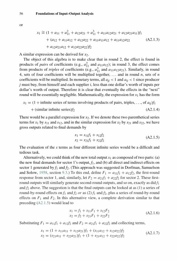
56 Foundations of Input–Output Analysis
or
x1 ∼= (1 + a11 + a211 + a12a21 + a3
11 + a11a12a21 + a12a21a11)f1
+ (a12 + a11a12 + a12a22 + a11a11a12 + a11a12a22 (A2.1.3)
+ a12a21a12 + a12a22a22)f2
A similar expression can be derived for x2.The object of this algebra is to make clear that in round 2, the effect is found in
products of pairs of coefficients (e.g., a211 and a11a12); in round 3, the effect comes
from products of triples of coefficients (e.g., a311 and a11a12a21). Similarly, in round
4, sets of four coefficients will be multiplied together, . . . and in round n, sets of ncoefficients will be multiplied. In monetary terms, all ajj < 1 and aij < 1 since producerj must buy, from himself and each supplier i, less than one dollar’s worth of inputs perdollar’s worth of output. Therefore it is clear that eventually the effects in the “next”round will be essentially negligible. Mathematically, the expression for x1 has the form
x1 = (1 + infinite series of terms involving products of pairs, triples, . . ., of aij)f1
+ (similar infinite series)f2 (A2.1.4)
There would be a parallel expression for x2. If we denote these two parenthetical seriesterms for x1 by s11 and s12, and in the similar expression for x2 by s21 and s22, we havegross outputs related to final demands by
x1 = s11f1 + s12f2x2 = s21f1 + s22f2
(A2.1.5)
The evaluation of the s terms as four different infinite series would be a difficult andtedious task.
Alternatively, we could think of the new total output x1 as composed of two parts: (a)the new final demands for sector 1’s output, f1, and (b) all direct and indirect effects onsector 1 generated by f1 and f2. (This approach was suggested in Dorfman, Samuelsonand Solow, 1958, section 9.3.) To this end, define F1 = a11f1 + a12f2, the first-roundresponse from sector 1, and, similarly, let F2 = a21f1 + a22f2 for sector 2. These first-round outputs will similarly generate second-round outputs, and so on, exactly as did f1and f2 above. The suggestion is that the final outputs can be looked at as (1) a series ofround-by-round effects on f1 and f2 or as (2) f1 and f2, plus a series of round-by-roundeffects on F1 and F2. In this alternative view, a complete derivation similar to thatpreceding (A2.1.5) would lead to
x1 = f1 + s11F1 + s12F2
x2 = f2 + s21F1 + s22F2(A2.1.6)
Substituting F1 = a11f1 + a12f2 and F2 = a21f1 + a22f2 and collecting terms,
x1 = (1 + s11a11 + s12a21)f1 + (s11a12 + s12a22)f2x2 = (s21a11 + s22a21)f1 + (1 + s21a12 + s22a22)f2
(A2.1.7)
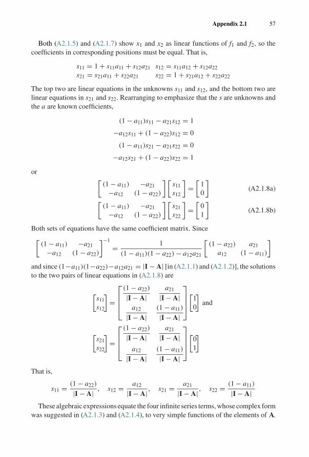
Appendix 2.1 57
Both (A2.1.5) and (A2.1.7) show x1 and x2 as linear functions of f1 and f2, so thecoefficients in corresponding positions must be equal. That is,
s11 = 1 + s11a11 + s12a21 s12 = s11a12 + s12a22
s21 = s21a11 + s22a21 s22 = 1 + s21a12 + s22a22
The top two are linear equations in the unknowns s11 and s12, and the bottom two arelinear equations in s21 and s22. Rearranging to emphasize that the s are unknowns andthe a are known coefficients,
(1 − a11)s11 − a21s12 = 1
−a12s11 + (1 − a22)s12 = 0
(1 − a11)s21 − a21s22 = 0
−a12s21 + (1 − a22)s22 = 1
or [(1 − a11) −a21
−a12 (1 − a22)
] [s11
s12
]=[
10
](A2.1.8a)[
(1 − a11) −a21
−a12 (1 − a22)
] [s21
s22
]=[
01
](A2.1.8b)
Both sets of equations have the same coefficient matrix. Since[(1 − a11) −a21
−a12 (1 − a22)
]−1
= 1
(1 − a11)(1 − a22) − a12a21
[(1 − a22) a21
a12 (1 − a11)
]and since (1−a11)(1−a22)−a12a21 = |I − A| [in (A2.1.1) and (A2.1.2)], the solutionsto the two pairs of linear equations in (A2.1.8) are
[s11
s12
]=
⎡⎢⎢⎣(1 − a22)
|I − A|a21
|I − A|a12
|I − A|(1 − a11)
|I − A|
⎤⎥⎥⎦[10
]and
[s21
s22
]=
⎡⎢⎢⎣(1 − a22)
|I − A|a21
|I − A|a12
|I − A|(1 − a11)
|I − A|
⎤⎥⎥⎦[01
]
That is,
s11 = (1 − a22)
|I − A| , s12 = a12
|I − A| , s21 = a21
|I − A| , s22 = (1 − a11)
|I − A|These algebraic expressions equate the four infinite series terms, whose complex form
was suggested in (A2.1.3) and (A2.1.4), to very simple functions of the elements of A.
58 Foundations of Input–Output Analysis
Moreover, these four simple functions are precisely the four elements of the Leontiefinverse, as found in (A2.1.1). In economic terms, the (I−A)−1 matrix captures in eachof its elements all of the infinite series of round-by-round direct and indirect effects thatthe new final demands have on the outputs of the two sectors. (A demonstration alongthese lines is much more complex for a three-sector input–output model and unwieldyfor more than three sectors.)
The elements of this Leontief inverse matrix are often termed multipliers. With
(I − A)−1 = L =[
l11 l12
l21 l22
]and forecasts for f1 and f2, the total effect on x1 is given
by l11f1+l12f2, the sum of the multiplied effects of each of the individual final demands.And similarly for x2. Input–output multipliers are explored in Chapter 6.
Appendix 2.2 The Hawkins–Simon Conditions
No matter how many terms we use in the series approximation to (I − A)−1in (2.17), itis clear that each of the terms contains only non-negative elements, since all aij ≥ 0. Asnoted in section 2.4, not only is A ≥ 0, but A2 ≥ 0, . . . , An ≥ 0; therefore (I+A+A2 +· · · ) is a matrix of non-negative terms. If the elements of f are all non-negative, then theassociated x will contain non-negative elements also. This is what one would expect;when faced with a set of non-negative final demands it would be meaningless in aneconomy to find that one or more of the necessary gross outputs were negative.23 For aLeontief system with A ≥ 0 and N (A) < 1 [so that the results in (2.17) hold], we knowthat negative outputs will never be required from any sector to satisfy non-negativefinal demands.
One could also explore conditions under which f ≥ 0 would always generate x ≥ 0by examining the general definition (I − A)−1 = 1
|I−A| [adj(I − A)] (Appendix A). Forthe simplest, two-sector case,
(I − A)−1 =
⎡⎢⎢⎣(1 − a22)
|I − A|a12
|I − A|a21
|I − A|(1 − a11)
|I − A|
⎤⎥⎥⎦and all of the elements in (I − A)−1 must be non-negative – the numerators must allbe non-negative and the denominator must be positive (the denominator must not bezero, either). Or, all numerators could be non-positive and the denominator negative.
We have already noted that aij ≥ 0 and that N (A) < 1 and (also by their defini-tion) all aij < 1.24 Thus all numerators in (I − A)−1 are non-negative. Therefore, if|I – A| > 0, all elements in the 2 × 2 Leontief inverse will be non-negative.
23 In some models, as we have seen, negative values could have meaning. When both x’s and f ’s are defined as“changes in”, namely �x and �f , then a result like �x3 = − 400 is interpreted as a decrease of $400 in sector3’s output.
24 As we saw in section 2.6, this need not be the case in input–output tables denominated in physical rather thanmonetary terms – for example, liters of input per kilogram of output. See also Chapters 9 and 10.
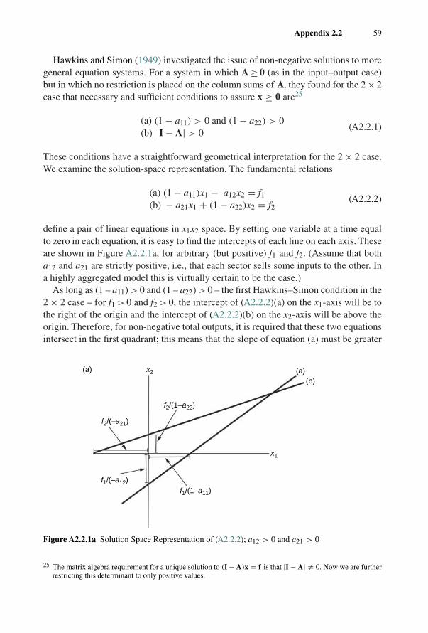
Appendix 2.2 59
Hawkins and Simon (1949) investigated the issue of non-negative solutions to moregeneral equation systems. For a system in which A ≥ 0 (as in the input–output case)but in which no restriction is placed on the column sums of A, they found for the 2 × 2case that necessary and sufficient conditions to assure x ≥ 0 are25
(a) (1 − a11) > 0 and (1 − a22) > 0(b) |I − A| > 0
(A2.2.1)
These conditions have a straightforward geometrical interpretation for the 2 × 2 case.We examine the solution-space representation. The fundamental relations
(a) (1 − a11)x1 − a12x2 = f1(b) − a21x1 + (1 − a22)x2 = f2
(A2.2.2)
define a pair of linear equations in x1x2 space. By setting one variable at a time equalto zero in each equation, it is easy to find the intercepts of each line on each axis. Theseare shown in Figure A2.2.1a, for arbitrary (but positive) f1 and f2. (Assume that botha12 and a21 are strictly positive, i.e., that each sector sells some inputs to the other. Ina highly aggregated model this is virtually certain to be the case.)
As long as (1 – a11) > 0 and (1 – a22) > 0 – the first Hawkins–Simon condition in the2 × 2 case – for f1 > 0 and f2 > 0, the intercept of (A2.2.2)(a) on the x1-axis will be tothe right of the origin and the intercept of (A2.2.2)(b) on the x2-axis will be above theorigin. Therefore, for non-negative total outputs, it is required that these two equationsintersect in the first quadrant; this means that the slope of equation (a) must be greater
f1/(1–a11)f1/(–a12)
f2/(–a21)
f2/(1–a22)
x2(a)
x1
(a)(b)
Figure A2.2.1a Solution Space Representation of (A2.2.2); a12 > 0 and a21 > 0
25 The matrix algebra requirement for a unique solution to (I − A)x = f is that |I − A| �= 0. Now we are furtherrestricting this determinant to only positive values.
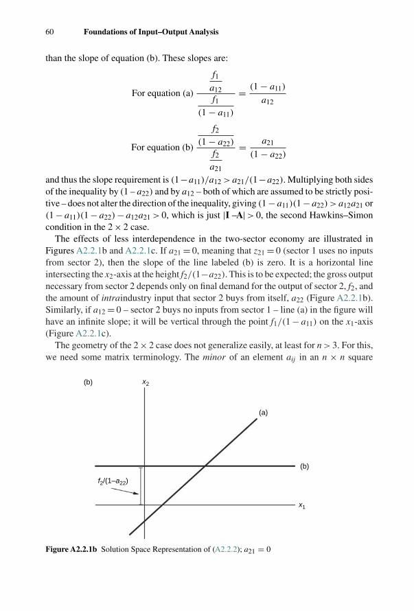
60 Foundations of Input–Output Analysis
than the slope of equation (b). These slopes are:
For equation (a)
f1a12f1
(1 − a11)
= (1 − a11)
a12
For equation (b)
f2(1 − a22)
f2a21
= a21
(1 − a22)
and thus the slope requirement is (1−a11)/a12 > a21/(1−a22). Multiplying both sidesof the inequality by (1 – a22) and by a12 – both of which are assumed to be strictly posi-tive – does not alter the direction of the inequality, giving (1 − a11)(1 − a22) > a12a21 or(1 − a11)(1 − a22) − a12a21 > 0, which is just |I –A| > 0, the second Hawkins–Simoncondition in the 2 × 2 case.
The effects of less interdependence in the two-sector economy are illustrated inFigures A2.2.1b and A2.2.1c. If a21 = 0, meaning that z21 = 0 (sector 1 uses no inputsfrom sector 2), then the slope of the line labeled (b) is zero. It is a horizontal lineintersecting the x2-axis at the height f2/(1−a22). This is to be expected; the gross outputnecessary from sector 2 depends only on final demand for the output of sector 2, f2, andthe amount of intraindustry input that sector 2 buys from itself, a22 (Figure A2.2.1b).Similarly, if a12 = 0 – sector 2 buys no inputs from sector 1 – line (a) in the figure willhave an infinite slope; it will be vertical through the point f1/(1 − a11) on the x1-axis(Figure A2.2.1c).
The geometry of the 2 × 2 case does not generalize easily, at least for n > 3. For this,we need some matrix terminology. The minor of an element aij in an n × n square
f2/(1–a22)
x2(b)
x1
(a)
(b)
Figure A2.2.1b Solution Space Representation of (A2.2.2); a21 = 0
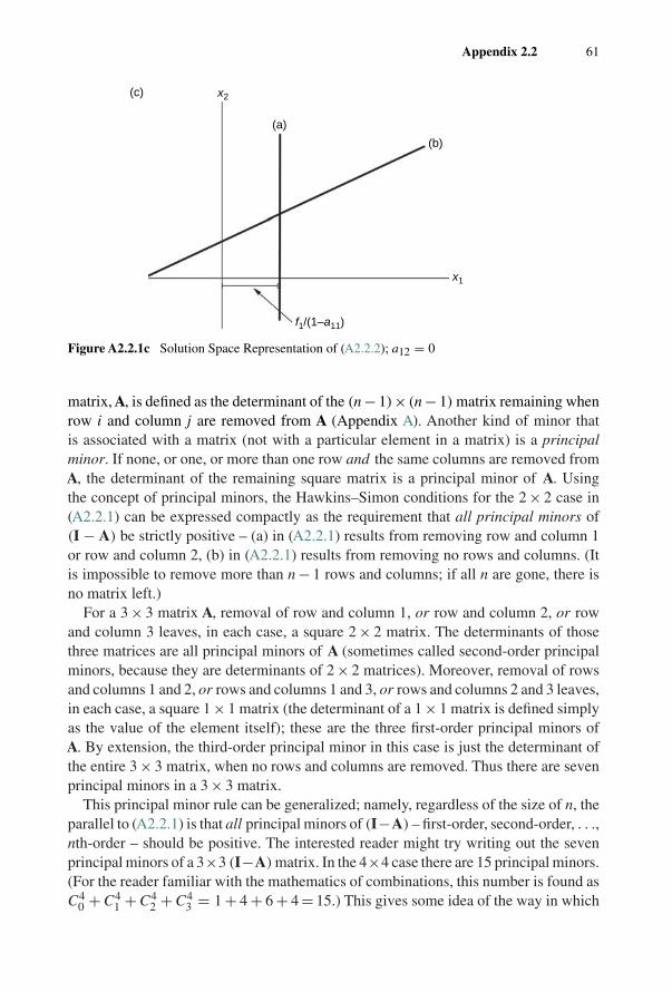
Appendix 2.2 61
f1/(1–a11)
x2(c)
x1
(a)
(b)
Figure A2.2.1c Solution Space Representation of (A2.2.2); a12 = 0
matrix, A, is defined as the determinant of the (n − 1)× (n − 1) matrix remaining whenrow i and column j are removed from A (Appendix A). Another kind of minor thatis associated with a matrix (not with a particular element in a matrix) is a principalminor. If none, or one, or more than one row and the same columns are removed fromA, the determinant of the remaining square matrix is a principal minor of A. Usingthe concept of principal minors, the Hawkins–Simon conditions for the 2 × 2 case in(A2.2.1) can be expressed compactly as the requirement that all principal minors of(I − A) be strictly positive – (a) in (A2.2.1) results from removing row and column 1or row and column 2, (b) in (A2.2.1) results from removing no rows and columns. (Itis impossible to remove more than n − 1 rows and columns; if all n are gone, there isno matrix left.)
For a 3 × 3 matrix A, removal of row and column 1, or row and column 2, or rowand column 3 leaves, in each case, a square 2 × 2 matrix. The determinants of thosethree matrices are all principal minors of A (sometimes called second-order principalminors, because they are determinants of 2 × 2 matrices). Moreover, removal of rowsand columns 1 and 2, or rows and columns 1 and 3, or rows and columns 2 and 3 leaves,in each case, a square 1 × 1 matrix (the determinant of a 1 × 1 matrix is defined simplyas the value of the element itself); these are the three first-order principal minors ofA. By extension, the third-order principal minor in this case is just the determinant ofthe entire 3 × 3 matrix, when no rows and columns are removed. Thus there are sevenprincipal minors in a 3 × 3 matrix.
This principal minor rule can be generalized; namely, regardless of the size of n, theparallel to (A2.2.1) is that all principal minors of (I−A) – first-order, second-order, . . .,nth-order – should be positive. The interested reader might try writing out the sevenprincipal minors of a 3×3 (I−A) matrix. In the 4×4 case there are 15 principal minors.(For the reader familiar with the mathematics of combinations, this number is found asC4
0 + C41 + C4
2 + C43 = 1 + 4 + 6 + 4 = 15.) This gives some idea of the way in which