Maximum Likelihood Estimation of Incomplete Data using Divergence Minimization An Information-Geometric Approach

Amin Zia

A course project for Convex Optimization and its Applications

Dec. 23, 2002 1- Introduction There is a large variety of problems requiring to find a probability distribution (PD) that best fits the evidence and a priori information. Obviously, a complete statistical characterization of evidences, e.g. likelihood function and posterior probability function in Bayesian inference, is crucial to probabilistic inference (PI). However, in most of the cases, this characterization is not available analytically and only realizations of it, like simulated data sets drawn from likelihood function or posteriors are available. In Maximum Likelihood (ML) estimation, it is desired to find the PD, P, among a family of distribution that best fits the observed data. However, there are situations that observed data is not sufficient statistics of the desired PD, and therefore, the problem is called “Incomplete-data ML estimation”. Examples of this general class of problems include Blind Channel Identification (in which the channel impulse response is estimated without any knowledge of input, learning in Hidden Markov Models (in which the hidden states are estimated using only the observations), State-space models (in which the state random variable is estimated using the observed variable), learning and estimation in Bayesian network (in which discrete or continuous hidden variables are estimated using the observed data), and error correction in algebraic decoders (in which optimum decisions made on the received noisy data based). Incomplete-data problem comes in different names depending on the nature of the problem including censored data, missing data and hidden data problems. The problem in shown to be NP-hard [7]. Therefore, any method that gives the approximate solution to the problem is valuable. In geometric approach to PI, the main idea is to consider a geometric interpretation for probability density (PD) measure spaces and treat the “Information divergence” also known as Kullback-Leibler (K-L) distance as a metric in this space. Based on this idea one can use well-known algebraic and geometric approaches to develop computational methods in PI. As a core to this approach, Information divergence (I-divergence) minimization (DM) is a well-known technique [1-6]. The nice feature in this approach is the ability to deal with entities based on their probabilistic behaviour rather than linear or nonlinear. In this report, a theoretical framework for solving the so-called “incomplete data problem” is given. The main approach used is a geometrical interpretation of probability measure spaces. For this purpose, the incomplete-data problem is expressed in a general framework as “divergence minimization, DM” between two PD convex sets. A lower bound for the objective function is obtained and using well-known theorems in information geometry, a detailed formulation for the algorithm giving the approximate solution is derived. In Section 2 basic definitions and theorems are given to provide the background and tools, which are necessary for developing the solution to Incomplete-data problem. In Section 3, after reviewing the general notion of maximum likelihood estimation and its relationship to DM, general statement of “incomplete data problem” is introduced. It is also shown that this specific problem can be modeled as a general DM problem between two convex sets. In Section 4, a specific formulation of MLE of Incomplete data is given in which the many-to-one mapping between complete and incomplete data assumed to be “probability marginal operator”. Based on this assumption, explicit formulations for both discrete random variables and Gaussian RVs’ are derived. In Gaussian RV case, interesting results provides simple method for estimating the closest positive definite matrix to a given initial positive definite matrix while satisfying marginal subspace constraints. In Section 5, the general incomplete problem while multiple observations are given is discussed. As an example, moreover, in Section 6 a simple blind channel identification problem is solved. For that part of minimization, i.e. minimizing a weighted-sum of log functions with linear equality constraints, that an analytical solution is not available, a type of Newton Method with a technique for eliminating the equality constraints a.k.a The Newton Step is used. The MATLAB implementation of the algorithms is also provided in appendix. This simple example clarifies the power of the method for solving similar and more complex problems in real world applications. In Section 7 a short note on the paper [8] is discussed. It is worth mentioning that the main purpose of this project has been to develop a theoretical framework, which can be used to solve many real-world problems. An application of the developed theories for Joint Channel Identification and Deconvolution as the future project currently under investigation based on the theories developed in this report is given in Section 9.

2- Preliminary definitions [2]: Let P , Q and R denote probability densities (PD) on a measurable space X. The I-divergence or Kullback-Leibler information distance, ( || )D P Q is defined as:

( )( || ) ( ).log( )x X

P xD P Q P xQ x∈

= ∑ (2.1)

This positive number provides a quantitative measure of how much P differs from . Q 2-1. I-projection: Given a PD , the set of PD’s Q

( , ) / ( || ) (0 )S Q P D P Qρ ρ ρ= < < ≤ ∞ (2.2) is called I-sphere with center Q and radius ρ . Now, if Γ is a convex set of PD’s intersecting with S Q , then ( , )∞

* min ( || )P

P D P Q∈Γ

= (2.3)

is called the I-projection of on . If such Q Γ *P exists, the convexity of Γ guarantees its uniqueness since

is strictly convex in . ( || )D P Q P 2-2. Existence of I-projection If the convex set of PD’s is variation-closed then each Q with S QΓ ( , )∞ Γ ≠∅∩ has an I-projection onΓ . The

convexity of guarantees the uniqueness of this projection, , since is strictly convex in . Γ *P ( || )D P Q P 2-3. General Alternating Minimization Technique [1-2]: Let Γ and be convex sets of PD measure on X. Also let Ω

(2.4) *

*

arg min ( || )

arg min ( || )Q

P

Q D P

P D P∈Ω

∈Ω

=

=

Q

Q

be the I-projections of on Γ and Q on P Ω respectively. Then if 0 , n n n nP Q 0∞ ∞= = be the sequence obtained by

alternating minimization of ( || )D P Q , starting from some 0P ∈Γ , then [2]:

,lim ( || ) inf ( || )n nn Q P

D P Q D→∞ ∈Ω ∈Γ

= Γ . (2.5) Ω

)= Γ Ω

Furthermore, if X is finite and and Ω are closed in the topology of pointwise convergence, then: Γ

* *( || ) ( ||nP P such that D P D→ Ω (2.6) This theorem guarantees that alternating projection between the two convex Γ and Ω sets converges to the minimum distance of the two sets. According to this theorem, iteratively projecting a PD onto the convex sets of PD’s converges to the I-projection of the PD on intersection of the sets.

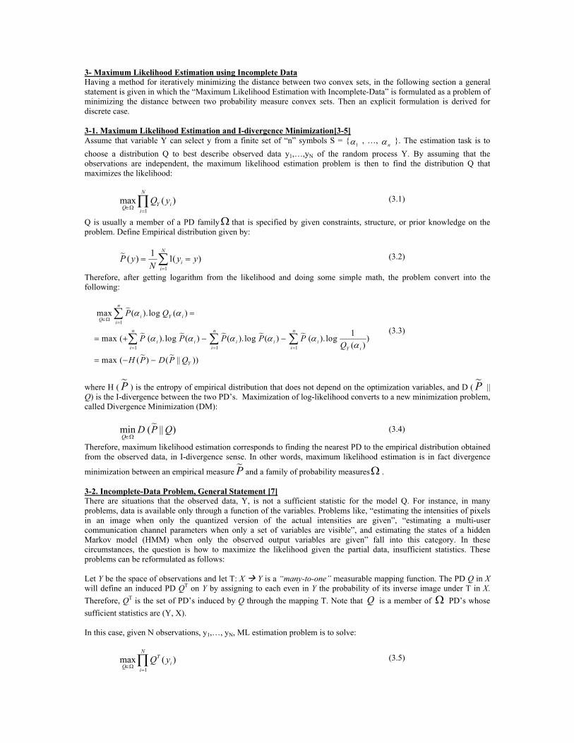
3- Maximum Likelihood Estimation using Incomplete Data Having a method for iteratively minimizing the distance between two convex sets, in the following section a general statement is given in which the “Maximum Likelihood Estimation with Incomplete-Data” is formulated as a problem of minimizing the distance between two probability measure convex sets. Then an explicit formulation is derived for discrete case. 3-1. Maximum Likelihood Estimation and I-divergence Minimization[3-5] Assume that variable Y can select y from a finite set of “n” symbols S = , …,

1α nα . The estimation task is to choose a distribution Q to best describe observed data y1,…,yN of the random process Y. By assuming that the observations are independent, the maximum likelihood estimation problem is then to find the distribution Q that maximizes the likelihood:

1

max ( )N

Y iQ i

Q y∈Ω

=∏ (3.1)

Q is usually a member of a PD family that is specified by given constraints, structure, or prior knowledge on the problem. Define Empirical distribution given by:

Ω

1

1( ) 1( )N

ii

P y y yN =

= ∑ = (3.2)

Therefore, after getting logarithm from the likelihood and doing some simple math, the problem convert into the following:

1

1 1 1

max ( ).log ( )

1max ( ( ).log ( ) ( ).log ( ) ( ).log )( )

max ( ( ) ( || ))

n

i Y iQ in n n

i i i i ii i i Y i

Y

P Q

P P P P PQ

H P D P Q

α α

α α α α αα

∈Ω=

= = =

=

= + − −

= − −

∑

∑ ∑ ∑ (3.3)

where H ( P ) is the entropy of empirical distribution that does not depend on the optimization variables, and D ( P || Q) is the I-divergence between the two PD’s. Maximization of log-likelihood converts to a new minimization problem, called Divergence Minimization (DM):

min ( || )Q

D P Q∈Ω

(3.4)

Therefore, maximum likelihood estimation corresponds to finding the nearest PD to the empirical distribution obtained from the observed data, in I-divergence sense. In other words, maximum likelihood estimation is in fact divergence

minimization between an empirical measure P and a family of probability measuresΩ . 3-2. Incomplete-Data Problem, General Statement [7] There are situations that the observed data, Y, is not a sufficient statistic for the model Q. For instance, in many problems, data is available only through a function of the variables. Problems like, “estimating the intensities of pixels in an image when only the quantized version of the actual intensities are given”, “estimating a multi-user communication channel parameters when only a set of variables are visible”, and estimating the states of a hidden Markov model (HMM) when only the observed output variables are given” fall into this category. In these circumstances, the question is how to maximize the likelihood given the partial data, insufficient statistics. These problems can be reformulated as follows: Let Y be the space of observations and let T: X Y is a “many-to-one” measurable mapping function. The PD Q in X will define an induced PD QT on Y by assigning to each even in Y the probability of its inverse image under T in X. Therefore, QT is the set of PD’s induced by Q through the mapping T. Note that Q is a member of Ω PD’s whose sufficient statistics are (Y, X). In this case, given N observations, y1,…, yN, ML estimation problem is to solve:

1

max ( )N

TiQ i

Q y∈Ω

=∏ (3.5)

Note that the optimization is done within a PD family setΩ , and so in X, but the criterion is optimized based on the image of the PD in Y. Therefore, as Y is not sufficient statistics of Q, and besides the mapping is a “many-to-one” type, there is no one-to-one correspondence between the optimization variable and the criteria. In fact, an infinitely large number of PD’s can be found that induce the same PD QT in observation space. Let’s define: / TP P PΓ = = (3.6)

Where P is defined as empirical distribution induced on Y by observations, as defined in (). Then we have:

: ( )

: ( )

: (

( )( || ) ( ).log( )( )( ).log( )

( ( ) ). ( / ( ) )( ( ) ). ( / ( ) ).log( ( ) ). ( / ( ) )

( ). ( / ( ) )( ). ( / ( ) ).log( ). ( / ( ) )

x X

x X x T x y

y Y x T x y

TT

Tx T x

P xD P Q P xQ x

P xP xQ x

P T x y P x T x yP T x y P x T x yQ T x y Q x T x y

P y P x T x yP y P x T x yQ y Q x T x y

∈

∈ =

∈ =

=

=

= == = =

= =

== =

=

∑

∑ ∑

∑ ∑

)

: ( )

/ /

( ) ( / ( ) )( ).log ( ) ( / ( ) ).log( ) ( / ( ) )

( || ) ( || / )

x X y

TT T

Ty Y x T x y

T T X Y X Y T

P y P x T x yP y P y P x T x yQ y Q x T x y

D P Q D P Q P

∈ =

∈ =

== + =

=

= +

∑ ∑

∑ ∑

where in fact, PT holds the information that is observed. The last term denotes the I-divergence between the conditional distributions on X, given Y. This equations clarify the relationship between the I-divergence in X and Y spaces. The first term on right in fact is an upper bound on the divergence. Now let’s fix Q∈Ω and try to minimize D P over all

PD’s . In other words, we are searching for a P in a family of PD’s whose images through T are( || )Q

P∈Γ P , i.e. Γ, which is closest to Q, in I-divergence sense. Obviously, the first term in RHS is the same for all P and the second term, which is non-negative, can be made to vanish by setting . Therefore we have: /X Y X YP Q= /

min ( || ) ( || ),T

PD P Q D P Q Q

∈Γ= ∀ ∈Ω

(3.7)

In this relationship Q is the family of desired PD’s in complete data space, QT is its image in observation space. The relationship reveals that the minimum I-diversity between any Q and the family of PD’s that satisfy the constraints defined Γ is unique and is the I-divergence between empirical distribution of observed data and the induced PD QT. It follows that the ML estimation defined in () reduces to the following problem:

arg min ( || )

arg min min ( || )

T

Q

Q P

Q D P Q

D P Q∈Ω

∈Ω ∈Γ

=

= (3.8)

Where therefore, the maximum likelihood estimation problem is to find the minimum I-distance between two PD family Γ and . In other words, a Q from a desired family of PD’s should be found that is closets to a family of PD’s whose members are the inverse image of empirical distribution of observations.

Ω

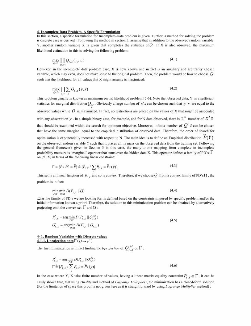
4- Incomplete Data Problem, A Specific Formulation In this section, a specific formulation for Incomplete-Data problem is given. Further, a method for solving the problem is discrete case is derived. Following the method in section 3, assume that in addition to the observed random variable, Y, another random variable X is given that completes the statistics of Q . If X is also observed, the maximum likelihood estimation in this is solving the following problem:

,( , )

max ( , )Y X i iQ x y

Q y x∈Ω∏ (4.1)

However, in the incomplete data problem case, X is now known and in fact is an auxiliary and arbitrarily chosen variable, which may even, does not make sense to the original problem. Then, the problem would be how to choose Q such that the likelihood for all values that X might assume is maximized:

,,

max ( , )Y XQ xx y

Q y x∈Ω

∑∏ (4.2)

This problem usually is known as maximum partial likelihood problem [5-6]. Note that observed data, Y, is a sufficient statistics for marginal distribution . Obviously a large number of QY 'x s can be chosen such that are equal to the

observed values while is maximized. In fact, no restrictions are placed on the values of X that might be associated

with any observation . In a simple binary case, for example, and for N data observed, there is 2 number of

'y s

N

Q

y 'x s

that should be examined within the search for optimum objective. Moreover, infinite number of Q can be chosen that have the same marginal equal to the empirical distribution of observed data. Therefore, the order of search for

optimization is exponentially increased with respect to N. The main idea is to define an Empirical distribution

' s

( )P Y on the observed random variable Y such that it places all its mass on the observed data from the training set. Following the general framework given in Section 3 in this case, the many-to-one mapping from complete to incomplete probability measure is “marginal” operator that sums over the hidden data X. This operator defines a family of PD’s Γ on (Y, X) in terms of the following linear constraint:

, , / / ( )TYY X Y X

xP P P P P P yΓ = = =∑ (4.3)

This set is an linear function of and so is convex. Therefore, if we choose from a convex family of PD’s,Y XP Q Ω , the

problem is in fact:

,min min ( || )Y XP QD P Q

∈Γ ∈Ω (4.4)

Ω as the family of PD’s we are looking for, is defined based on the constraints imposed by specific problem and/or the initial information known a priori. Therefore, the solution to this minimization problem can be obtained by alternatively projecting onto the convex set and : Γ Ω

*, ,

* *, ,

arg min ( || )

arg min ( || )

oldY X Y X Y XP

Y X Y X Y XQ

P D P

Q D P∈Γ

∈Ω

=

=

,

,

Q

Q (4.5)

4- 1. Random Variables with Discrete values 4-1-1. I-projection ontoΓ (Q P )*→

The first minimization is in fact finding the I-projection of Q on,oldY X Γ :

*, ,arg min ( || )old

Y X Y X Y XPP D P

∈Γ= ,Q

y

, , / ( )YY X Y Xx

P P PΓ =∑ (4.6)

In the case where Y, X take finite number of values, having a linear matrix equality constraint , it can be

easily shown that, that using Duality and method of Lagrange Multipliers, the minimization has a closed-form solution (for the limitation of space this proof is not given here as it is straightforward by using Lagrange Multiplier method) :

,Y XP ∈Γ

*, / .old

YY X X YP Q P= (4.7)

Therefore: * /, , /

, ,

.( || ) . .log

.log ( ) log ( )

YX YYY X Y X X Y

y x Y X

YY Y Y

y yY

Q PD P Q Q PQ

PP H PQ

=

= = − −

∑

∑ ∑ Q y

(4.8)

Hence, by approaching iteratively by projecting to it and minimizing this distance, the likelihood of observed data is maximized.

Γ

4-1-2. I-projection ontoΩ ( P Q )*→ The second minimization, moreover, can be done by assuming that the complete data statistics is known, i.e. *

,Y XP . The

problem specifically is to solve:

* *, ,

*, ,

,

arg min ( || )

arg max .log( )

Y X Y XQ

Y X Y XQ Y X

Q D P Q

P Q∈Ω

∈Ω

=

= ∑ (4.9)

, , / Y X Y XQ Q satisfy constriants defined by aperiori iformation or imposed by problemΩ =

In fact, this is a general ML estimation problem assuming that the Empirical Distribution for complete data i.e. *,Y XP is

given. Convex constraint set is usually defined by apriori information in hand and/or the specific structure of the problem being solved.

Ω

4-2. Random Variables with Gaussian PD’s 4-2-1. I-projection ontoΓ ( Q P )*→

Another class of interest is signals with Gaussian PD. Consider the zero-mean Gaussian distributions on : n

1

1/ 2

det( ) 1( ) .exp( )(2 ) 2

TQ n

QN z z Q z

π

−−= − (4.10)

where z =(y, x) is complete statistics of desired PD’s and Q is covariance matrix of complete data. Now, assume that n is partitioned into two sets Y and X. For instance, assume that Y (observations) corresponds to dimensions 1, 2, …, r and that X (inaccessible data) corresponds to r+1, …, n. We can write Q is block form:

11 12

21 22

Y X

Q QQ

Q Q

=

and (4.11) 11 121

21 22

Y X

Q QQ

Q Q−

=

Now for any 0YP , consider Gaussian density PN on corresponding to subspaceY , the observed subspace.

Therefore, the marginal of

r

( )QN z corresponding to subspace Y isQ . We have: 11

11

*, /

111 12 221

11

111111 121

21 22

. .

exp ( 2 ) .exp ( )exp ( )

:

( )

Y

QYY X X Y P

Q

T T TT

YT

A

Y

T

NP Q P N

N

y Q y y Q x x Q x y P yy Q y

N where

Q Q P QA

Q Q

−

−

−−−

= =

− + +=

−=

− + =

− (4.12)

Therefore, givenQ , one can calculate1,Y X−

1A− by simply adding 1 1

11( )YP Q− −− to the upper left block.

4-2-2. I-projection ontoΩ ( ) *P Q→This projection corresponds to solving the complete data ML estimation problem for a jointly Gaussian RV’s (Y,X) using conventional optimization techniques. Following the same path we did in the discrete case, by assuming that the

complete data statistics is known, i.e. , the problem specifically is to solve: *,Y XP

* *

, ,

*, ,

,

arg min ( || )

arg max .log( )

Y X Y XQ

Y X Y XQ Y X

Q D P Q

P Q∈Ω

∈Ω

=

= ∑ (4.13)

, , / .Y X Y XQ Q is a join tly Gaussian distributionΩ =

In fact, this is a general ML estimation problem assuming that the Empirical Distribution for complete data i.e. is

given. Convex constraint setΩ is usually defined by a priori information in hand and/or the specific structure of the problem being solved. Specifically:

*,Y XP

* 1

,1

1arg max log det( )

: 0

NT

Y X iQ iQ Q

Nsubject to Q

−

=

= −

>

∑ 1z Q z−i (4.14)

11

/ 2

det( ) 1( ) .exp( )(2 ) 2

TQ n

QN z z Q z

π

−−= −

1−

(4.15)

Let R , the problem would be a “maximum determinant-problem” that can be solved with [9]: Q=

* 1, arg min log det( ) ( )

: 0Y X R

R R

subject to Q

−=

>

Tr SR+ (4.16)

where S is the complete-data Covariance matrix obtained from the last projection operation:

1

1 .N

Ti i

iS z z

N =

= ∑ A=

S

(4.17)

The problem in this form an be solved analytically and has the closed-form solution:

* * 1, ( )

: 0Y XQ R

subject to Q

−= =

> (4.18)

This is very interesting result. In fact, this shows that in case of having Gaussian distribution for complete data, the only iteration needed is the first projection.

Result 1: Therefore, assume start fromQ , the iterative projection onto the observation subspace (incomplete data) converges to towards the maximum likelihood of complete data:

0

1 1

0 0 1 1 0 1 ... * * arg min min ( || )Q P

Q A P Q A A P Q D P Q− −

∈Ω ∈Γ→ → = = → → → = = (4.19)

This is a rather important proposition that can be used is several applications where the observed Gaussian data is not statistically sufficient for ML estimation. Result 2: Given iteratively applying the projection (4.12) will end up with another that is closest to

and agrees with Y subspace Q (Incomplete or observed subspace).

0Q > 0P > Q

5- Incomplete Data, Gaussian PS’s and Multiple Observations So far, it is assumed that only one set of observations are in hand and so only one marginal constraint should be satisfied for the projections. It is proved, then, that for discrete variable case projection (Q ) is: *P→

*, ,arg min ( || )old

Y X Y X Y XPP D P

∈Γ= ,Q (5.1)

*, / .old

YY X X YP Q P=

However, in case we have more than one observation data sets, we may extent the results we derived to find the best PD that both is closest to a family of PD’s and agrees with multiple marginal constraints. In what follows it is assumed that the PD’s are Gaussian and therefore, only 1st projection is needed (Q ) to minimize*P→ ( || )D P Q . For clarity

in notations we first define a mapping operator , ( )X PM Q as the operator that transfers into a new distribution

whose X-marginal is

Q

P . By this definition, the projection (Q ) is denoted by: *P→

*, , (

Y

oldY X X YX PP M Q= / ) (5.2)

However, in case there are K sets of observations available, the method confirms that the estimated PD’s satisfy all the marginal constraints. More formally, let

1,..., kK i i= be subset of the dimensions 1, 2, …, n. Then, the operator

, ( )K PM Q transforms into a new PD whose K-marginal exactly matchesQ P . In fact, the pair ( , )iiK P is a constraint

on the behavior of the desired distribution. Therefore, given a starting distribution Q and a collection

1 21 2( , ( , )mm( , ), ),...,K P K P K P of these pairs, one can use iterative application on mapping operator , ( )iKi PiM Q to

find the closest PD to the family and whose marginal agree with the empirical distributions QΩ= :1...:i mP obtained from the observations.

6- Simulation Results, Blind Discrete Channel Identification, A Simple Application A simple application of Incomplete-data problem for discrete RV case is investigated. Given N observations,

, from the output of the discrete channel , and no other information about the input. The RV

select symbols from 5-symbol vocabulary (n = 5). Obviously, Y is not sufficient statistics for estimating1, , Ny … y ( / )P Y X

( / )P Y X .

However, using the method developed so far, with the following assumptions for projection *P Q→ :

, /Y XQ constrains defined by structureof likelihood functionΩ = (6.1)

The problem can be solved and the PD whose marginal distribution best agree with the observed data is found. It is guaranteed that in each iteration, the likelihood of data is increased, and therefore, having a good initial point for the optimization, reaching to local optimum is guaranteed. As shown in Section 4.1. the first projection, i.e.Q , has a closed form. The second iteration, P , is also in a convex optimization problem with convex constraint set. In this application, we examined some linear constraints on Q. Therefore, a type of Newton Method with a technique for eliminating the equality constraints a.k.a The Newton Step [10, Section 9.3] is used.

*P→*Q→

In the first scenario, it is assumed that we constraint Q to be symmetric:

/ ( , ) 1

( , ) 0

x y

T

Q q y x

Q Qq y x

Ω = =

=≥

∑∑ (6.2)

Assuming a random initial value for Q and channel estimate P(Y,X): Q initial = 0.0638 0.0685 0.0194 0.0118 0.0640

0.0174 0.0473 0.0709 0.0488 0.0638 0.0007 0.0100 0.0600 0.0315 0.0653 0.0539 0.0504 0.0254 0.0122 0.0114 0.0140 0.0310 0.0628 0.0359 0.0598

The final value for estimated Q is: Q final = 0.0897 0.1229 0.0630 0.0537 0.0499

0.1229 0.0117 0.0161 0.0193 0.0194 0.0634 0.0161 0.0342 0.0324 0.0177 0.0539 0.0197 0.0326 0.0224 0.0197 0.0494 0.0199 0.0176 0.0194 0.0131

As can be seen the estimated Q is closely symmetric as: Q - Q' = 1.0e-003 *

0 -0.0000 -0.4046 -0.1876 0.5103 0.0000 0 0.0480 -0.3864 -0.5083 0.4046 -0.0480 0 -0.1646 0.0506 0.1876 0.3864 0.1646 0 0.3239 -0.5103 0.5083 -0.0506 -0.3239 0

Figure 1. shows the empirical distribution of observed data as well as the y-marginal initial value of channel PD. Figure 2. shows the final values after convergence.

Figure 1 Figure 2 Figure 3and 4 show the I-distance between P and Q and the -Log-likelihood of Incomplete data within the convergence:

Figure 3 Figure 4 Obviously, after estimating the joint PD of Y and X we can calculate the channel transmission matrix:

( / ) ( , ) / YP X Y P X Y P= (6.3)

As another example, assume that we imposed the following constraints on Q :

/ ( , ) 1

( , ) 1/

( , ) 0

x y

y

Q q y x

q y x N

q y x

Ω = =

=

≥

∑∑

∑ (6.4)

Based on this assumption, the estimated Q should have uniformly distributed x-marginal and y-marginal equal to the empirical distribution. Figure 5. shows the empirical distribution of observed data as well as the y-marginal initial value of channel PD. Figure 6. shows the final values after convergence.

Figure 5 Figure 6 Figures 7 and 8 show the I-distance between P and Q and the -Log-likelihood of Incomplete data within the convergence:

Figure 7 Figure 8 Figure 9 shows the imposed x-marginal constraints as well as the x-marginal final value of channel PD.

Figure 9 For the last example, assume that we impose a contradictory constraint on Q. In this case, we consider both constraints for the last two examples. The symmetric Q should have the same marginal distributions on X and Y. Therefore, imposing a uniform distribution on x-marginal while the y-marginal is the given empirical distribution makes algorithm unable to converge properly. Figures 10 and 11 show the Y and X-marginal distributions of estimated distribution that approximately fit the Y-marginal given by incomplete data and X-marginal imposed by the constraints. It can be seen

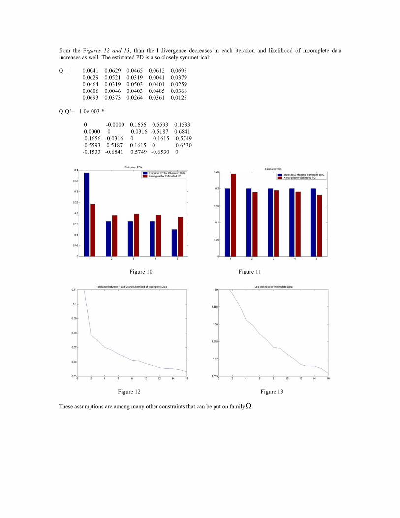
from the Figures 12 and 13, than the I-divergence decreases in each iteration and likelihood of incomplete data increases as well. The estimated PD is also closely symmetrical: Q = 0.0041 0.0629 0.0465 0.0612 0.0695

0.0629 0.0521 0.0319 0.0041 0.0379 0.0464 0.0319 0.0503 0.0401 0.0259 0.0606 0.0046 0.0403 0.0485 0.0368 0.0693 0.0373 0.0264 0.0361 0.0125

Q-Q’= 1.0e-003 *

0 -0.0000 0.1656 0.5593 0.1533 0.0000 0 0.0316 -0.5187 0.6841 -0.1656 -0.0316 0 -0.1615 -0.5749 -0.5593 0.5187 0.1615 0 0.6530 -0.1533 -0.6841 0.5749 -0.6530 0

Figure 10 Figure 11

Figure 12 Figure 13 These assumptions are among many other constraints that can be put on familyΩ .

7- A Short note on [8]: Apart from an overview of geometric approach to probabilistic inference, the main contribution of the [8] is to provide an Iterative Minimization algorithm. Given a finite set of observations, say K, and assuming the inverse image of the observations through the many-to-one mapping ( ( ) ( . ) [8]Y i i iP P in this report and F m q f in= =T ) partitions the complete-data probability measure space, say Γ , one can simplify the divergence minimization problem [8, equation 10] into simpler one [8, equation 30]. This simplification is a natural consequence of the method provided in Section 3 assuming a partitioned . After this simplification, the problem is to find the minimum divergence between a desired set of PD’s, say , and

ΓΩ 1,..., KΓ Γ iteratively. The convergence of this method is guaranteed by Csiszar [2].

8- Conclusion and future work: In this project after introducing notions of information geometry, divergence minimization and the theorems addressing the iterative methods for minimizing the I-divergence between two convex probability measure sets, it is shown that the incomplete-data problem can be seen as minimization of I-divergence between two convex families of probability distributions. The problem is solved for two special case i.e. random variables with discrete values and random variables with Gaussian distribution. It is shown that in the former case, the first projection from the family of desired distributions onto the constraint PD set has an analytical solution. The second projection from the constraint set onto the desired PD set was also solved using a type of Newton method eliminating the equality constraints and Newton step. It is also shown that in Gaussian case, analytical solution came up with an interesting result for finding the nearest positive definite matrix to a given positive definite matrix that agrees with the subspace corresponding to incomplete or observed subspace. Finally, a general case for MLE with multiple observations was discussed. A simple channel identification for discrete case was also solved using the developed methods. A short discussion on paper [8] was also presented which showed that the main contribution of the paper is basically a consequence of theorems approved by Csiszar [2]. The method presented in this report is going to be used to solve a Blind MISO Channel Identification. It can be shown that having a set of training sequence of inputs and output observations ML estimation of the channel gains can be obtained using least square method provided that the training sequence matrix has full column rank. However, in cases which no training sequence is available, the methods of alternating projection can be used for maximum likelihood estimation of channel matrix. It can be shown that this problem fits into the general framework provided in Section 5 and therefore, an iterative method can be obtained to iteratively update the covariance matrix of complete data as new observation data is arrived. Obviously, the parameters of the channel matrix can be derived from the covariance matrix of complete data (More information can be provided on this application). 9- Reference: [1] T. Cover, J. Thomas, Elements of Information Theory, 1996. [2] I. Csiszar, “I-divergence geometry of probability distribution and minimization problems,” Ann. Probab., vol. 3, pp. 146-158, 1975. [3] I. Csiszar, “Information Theoretic Methods in Probability and Statistics”, Budapest, 2001. [4] I. Csiszar, “A Geometric Interpretation of Darroch and Ratcliff’s Generalized Iterative Scaling,” The Annals of Statistics, vol. 17, no. 3, pp. 1409-1413, 1989. [5] W. Byrne, “Information Geometry and Maximum Likelihood Criteria,” Proceeding of Conference on Information Sciences and Systems, Princeton, NJ, 1996. [6] S.I. Amari, Differential-Geometrical methods in Statistics, Springer-Verlag, New York, 1985. [7] A. P. Dempster, A.M. Laird, and D. B. Rubin, “Maximum Likelihood from Incomplete data via the EM Algorithm,” J. Royal Stat. Soc., Sec. B, vol. 39, no. 1, pp. 1-38, 1977. [8] T.H. Chan, and et al. “Geometric Framework for Probabilistic Inference using Divergence Measure,” University of Toronto. [9] L. Vandenberghe, S. Boyd, and S.-P. Wu, “Determinant maximization with linear matrix inequality constraints” (http://www.stanford.edu/~boyd/maxdet.html). [10] S. Boyd, L. Vandenberghe, Convex Optimization, (http://www.stanford.edu/~boyd/cvxbook.html).

Appendix: MATLAB Code, Section 6. % This program is an implementation of Alternating Projection Method for solving Incomplete-Data problem % Dec 2002, Amin Zia % Functions: % projection1() minimizes D(P || Q) for P given Q_old % projection2() minimizes D(P || Q) for Q given P_old % marginal_over_y() calculates the marginal distribution over y % Idist() calculates the K-L distance between two distributions clear all close all % scenario n = 5; % symbol set cardinality % empirical distribution of p(y) p_channel = rand(n,n) p_channel = p_channel/sum(sum(p_channel)); px0 = rand(n,1); py1 = p_channel_real*px1; py1 = py1/sum(py1); py0 = py1; % initilzation % initilizing the channel p(x,y) p0 = rand(n,n) p_initial = p0 / sum(sum(p0)); % tolerance for difference between I-divergence between the iterations Itolerance = 1e-10; % main loop t = 0; p_old = p_initial; Idist1 = 10; Idist2 = 9.99; for i = 1:1000 if (Idist1 - Idist2) < Itolerance display('thats enough') break else t = t+1; % Q --> P* p = projection1(p_old, py0); % P --> Q* q = projection2(p, py0); q = q/sum(sum(q)); p_old = q; Idist1 = Idist2; % I-distance checking Idist2 = Idist(p, q); Idist_pq(t) = Idist2; % saving the x-marginal trend s = 0; q_marginal = sum(q)'; for jj=1:length(py1) s = s - py1(jj)*log(q_marginal(jj)); end like_q(t) = s; end end save results.mat

%%%%%%%%%%%% projection 1 %%%%%%%%%%%%% function [p]= projection1(p_old, py0) % py0 : empirical distribution of marginal for p(y) n = length(p_old); for i = 1:n, s(i) = 0; end for j = 1:n for i = 1:n s(j) = s(j) + p_old(i, j); end end for i = 1:n for j = 1:n p(i, j) = (p_old(i, j)/s(j)) * py0(j); end end %%%%%%%%%%%%%%% projection 2 %%%%%%%%%%%%%%%%%% % This function implements the projection of P on family containing Q. % Functions: % mle() maximum likelihood estimation using complete data (p) % Dec 2002, Amin Zia function [q]= projection2(p, py0) % mstep(p) % p: the old p from projection1 % py0: empirical distribution of incomplete data n = length(p); k = py0; q = mle(p, k); % solves a two-dim-indexed problem %%%%%%%%%%%% maximum likelihood estimation %%%%%%%%%%%% function [q] = mle(pij, py) % pij: the complete data from projection1. p = pij; % vectorizaing the 2-dim pdf p n = length(p); r = 0; for i = 1:n for j = 1:n r = r+1; a(r) = p(i, j); end end a = a'; % vectorized empirical distribution for complete data % the narginals should be re-formed into proper form of A.x = b % B: coefficient matrix for x-marginals % C: coefficient matrix for y-marginals % re-forming the 2-dim coefficients for constraints into linear % constraints for 1-dim variable vector % implemeting B.x = x-marginals of q for i = 1 for j = 1:n B(i, j) = 1; end for j = n+1 : n^2 B(i, j) = 0; end end for i = 2:n-1 for j = 1 : (i-1)*n

B(i, j) = 0; end for j = (i-1)*n+1 : (i-1)*n+n B(i, j) = 1; end for j = (i-1)*n+n+1 : n^2 B(i, j) = 0; end end for i = n for j = n^2-n : n^2 B(i, j) = 1; end for j = 1: n^2-n B(i, j) = 0; end end for i = n for j = (i-1)*n + i B(i, j) = 1; end for j = 1: n^2-n B(i, j) = 0; end end % implemeting B.x = y-marginals of q for i = 1:n for j = 1:n^2; C(i, j) = 0; end end for i = 1:n for j = 0: n-1; C(i, j*n+i) = 1; end end % imposing Symmetric contraints on channel for i = 1:2*n for j = 1:n^2; D(i, j) = 0; end end D(1, 2) = 1; D(1, 6) = -1; D(2, 3) = 1; D(2, 11) = -1; D(3, 4) = 1; D(3, 16) = -1; D(4, 5) = 1; D(4, 21) = -1; D(5, 8) = 1; D(5, 12) = -1; D(6, 9) = 1; D(6, 17) = -1; D(7, 10) = 1; D(7, 22) = -1; D(8, 14) = 1; D(8, 18) = -1; D(9, 15) = 1; D(9, 23) = -1; D(10, 20) = 1; D(10, 24) = -1; for i = 1:n^2 D(11, i) = 1; end % alternatively estimation using several constraints % main loop for i = 1:3 if i ==1 x = a; end

% estimating with uniformly distributed x.marginal constraint A = B; b = [1/n 1/n 1/n 1/n 1/n]'; [x, f] = newton(x, A, b); x = x/(sum(x)); % estimating with symmetricity constraint l = [0 0 0 0 0 0 0 0 0 0 1]'; A = D; b = l; [x, f] = newton(x, A, b); x = x/(sum(x)); end % re-arranging into 2-dim PDF r = 0; for i = 1:n for j = 1:n r = r+1; q(i, j) = x(r); if q(i, j) < 0 display('Newton method should be repeated!') end end end %%%%%%%%%%% newton method %%%%%%%%%%%%%% function [x, f] = newton(a, A, b) % Newton Method for Solving a convex optimization problem with % differentiable nonlinear objective and linear equality constraints % Amin Zia % Dec. 2002 % Algorithm is using the elimination method for including the euality % contrtaints into the feasible Newton steps. % The step size calculation is based on Backtracking method. % Functions % Obj() objective function % hessn() hessian % grt() gradiant % initialization % tolerance factor e = 0.1; % backtracking parameter 0 < alfa < 0.5 alfa = 0.2; % backtracking parameter 0 < beta < 1 beta = 0.05; % initial point for the algorithm: for i = 1:100, x = A\b; if min(x) >= 0 display('initial point ok'); break; end display('negative initial point'); end % preventing singularities for i = 1:size(x) if x(i) == 0; x(i) = 1e-3*rand; end end for i = 1:100 % gradiant and hessian of x

g = grt(x, a); h = hessn(x, a); % Compute the Newton Step by solving a second-order dual problem % vnt = -(inv(h) - inv(h)*A_t*inv(A*inv(h)*A_t)*A*inv(h)) * g % h = hessian, g = gradiant v = -(inv(h) - inv(h) * A' * inv(A*inv(h)*A') * A * inv(h)) * g; % Compute the optimiality criterion coefficient (aka Newton decrement): % lambda = sqrt(g_t * inv(h) * g) lambda = sqrt(g' * inv(h) * g); % quit if lambda^2 /2 is less than a tolerance e>0 if (lambda^2/2 > e) if i == 1 t = 0.01; f2 = obj(x + t*v, a); f1 = obj(x, a); end f2 = obj(x + t*v, a); f1 = obj(x, a); % computing the step size t using backtracking line search method t = 1; while (f2 > (f1 + alfa*t*g'*v)) t = beta*t; f2 = obj(x + t*v, a); f1 = obj(x, a); end if (t<=0) & (f2 > f1) display('there is no step size, the algorithm does not converge! :)') return else display('step size found') end % update the new variable value xold = x; x = x + t*v; for i = 1:length(x) if x(i) <= 1e-15*max(nonzeros(x)) x(i) = 0; end else x = xold; f = obj(x, a); return end end display('no convergence') %%%%%%%%%%%%%% objective function %%%%%%%%%%%%%%% function f = obj(x, a) % weighted sum of log functions f = 0; for r = 1:size(x) if x(r) <= 1e-10 xt = 1; else xt = x(r); end f = f - a(r)*log(xt); end %%%%%%%%%%%%%%% hessian function %%%%%%%%%%%%%%%%%%%% function hes = hessn(x, a)

% hessian for weighted sum of log functions for r = 1:length(x) if x(r) == 0 h(r) = 0; else h(r) = a(r)/x(r)^2; end end for r = 1:length(x) if x(r) == 0 h(r) = min(nonzeros(h)); end end hes = diag(h'); %%%%%%%%%%%%%%% gradiant function %%%%%%%%%%%%%%%%%% function gr = grt(x, a) % gradiant for weighted sum of log functions for r = 1:length(x) if x(r) == 0; g(r) = 0; else g(r) = - a(r) / x(r); end end for r = 1:length(x) if x(r) == 0; g(r) = max(nonzeros(g)); end end gr = g'; %%%%%%%%%%%%% I-distance function %%%%%%%%%%%%%%%%%%% function [Id] = Idist(p, q) n = length(p); Id= 0; for i = 1:n for j = 1:n if p(i, j) <= 0 pij = 1; else pij = p(i, j); Id = Id + pij*log(pij/q(i, j)); end end end