AN ANALYSIS OF THE DETERMINANTS OF THE ECONOMIC GROWTH RATE

IN KIRIBATI

by

Toani Barao Takirua

A thesis submitted in partial fulfillment of the requirements for the degree of Master of Arts

School of Economics Faculty of Business and Economics The University of the South Pacific

FEBRUARY 2008

© Toani B Takirua 2008

ii

AN ANALYSIS OF THE DETERMINANTS OF THE ECONOMIC GROWTH RATE

IN KIRIBATI

iii

DECLARATION OF ORIGINALITY

I, Toani B Takirua, declare that this thesis is my own work, and that to the best of my

knowledge, it contains no material previously published, or substantially overlapping

with materials submitted for the award of any other degree at any institution, except

where due acknowledgement is made in the text.

Toani B Takirua

iv

ACKNOWLEDGEMENTS

I acknowledged with thanks the endless valuable assistance rendered by Professor

Bhaskhara (Bill) Rao, of the School of Economics of the University of the South

Pacific, during my work on the thesis. Without his guidance this thesis couldn’t have

been completed in time.

I also wish to thank Associate Professor Biman Chand Prasad, Head of the School of

Economics of the University of the South Pacific, for his suggestions on an earlier draft

of the thesis. Remaining errors are my own.

In addition, I thank the Government of Kiribati for providing my in-service training and

the Government of New Zealand for its funding assistance, which led to the completion

of my Master of Art programme at the University of the South Pacific in Fiji.

Last but not the least, I cannot forget the never-ending valuable support from my family

and especially by my wife, Ngarone Metai, during the preparation and finalization of

this thesis.

Toani B Takirua

v

ABSTRACT

Kiribati is one of the least developed countries. With her increasing population, coupled

with its poor resource endowment (with the exception of having huge Exclusive

Economic Zone), the lack of foreign direct investment and the under-development of

the private sector, create financial burden to the Government. Foreign exchange

earnings from official development assistance, access fee, the revenue equalization

reserve fund (RERF) and the remittances are significant to the economy. Only the

RERF and the access fee have direct contribution to government revenues for its

recurrent and development budgets. Aid and the remittances are channeled to

unproductive investment and consumption and trade has been in a deficit. The growth

accounting result shows that factor accumulation contributes much to growth than the

total factor productivity (TFP). In econometric empirical analysis, none of the shift

variables (aid, remittances and export) have permanent effects on output, except export

having an effect in the short run.

vi

TABLE OF CONTENTS

Declaration of originality ( iii ) Acknowledgements ( iv ) Abstract ( v ) Table of Contents ( vi ) List of Tables and Figures ( viii ) Chapter 1. Introduction 1-6 1.1. Disparity in economic growth and some constraints 1.2. Purpose of study 1.3. Contents of the thesis 1.4. Conclusion Chapter 2. Background information on Kiribati and its economy 7-23 1. Introduction 2. Geography,Government,Population and Religions 3. Macroeconomic indicators 3.1. Government current account 3.2. Gross domestic product, Average growth rates and Inflation 3.3. Trade Liberalisation 3.4. GDP per capita and Employment 4. Major foreign exchange earnings 4.1. Fishing access fee 4.1. Revenue equalisation reserve fund (RERF) 4.2. Remittances 4.3. Official development assistance or aid 4.4. Gross national income per capita 5. Conclusion Chapter 3. Theories of economic growth 24-39 1. Introduction 2. Economic Growth Theories 2.1. A brief look at Harrod-Domar model 2.2. Solow model 2.2.1. Specifications of the Solow Model 2.2.1.1. Defining capital value 2.2.1.2. Defining value and growth output 2.2.1.3. Growth in labour force and technical progress

vii

2.2.1.4 Usefulness of growth accounting 3. The MIRAB economies and growth model 3.1. What is the MIRAB? 3.1.1. A re-look at the MIRAB model 3.2. Examining the relevancy of growth models 4. Conclusion Chapter 4. Data 40-52 1. Introduction 2. Definitions, data sources, analysis of data, methods to analyse data 2.1. Nominal and Real GDP 2.2. Real GDP growth rates 2.3. Estimating capital 2.4. Real capital growth rates 2.5. Labour force 2.6. Official Development Assistance - AID 2.7. Remittance 2.8. Real export earnings from copra 2.9. Method for analyzing data 3. Conclusion Chapter 5. Growth accounting 53-60 1. Introduction 2. Definitions 2.1. What is growth accounting? 2.2. What is factor accumulation? 2.3. What is total factor productivity? 3. Growth accounting results 4. Conclusion Chapter 6. Solow model and its extensions 61-77 1. Introduction 2. Unit roots and cointegration 2.1 Cointegration 3. The model 4. Empirical results 4.1. The Solow model with GETS 4.2. The Solow model with JML VECM 5. Extension to the Solow model

viii

5.1. GETS results with export ratio 5.2. GETS result with aid 5.3. GETS result with remittances 5.4. AD hoc specification 6. Conclusion Chapter 7. Conclusion 78-84 1. Introduction 2. Summary of quantitative results 3. Some data limitations 4. Additional observations 5. Recommendations References 85-94 Appendix 95-104

LIST OF TABLES AND FIGURES

Chapter 2. Figure 1. Map of Kiribati Figure 2. Religions Figure 3. Government expenditures Figure 4. Pattern and composition of government revenues Figure 5. GDP per capita Figure 6. Number of paid employees Figure 7. Access fee revenue Figure 8. Growth in RERF real value Figure 9. GNI per capita Chapter 4. Figure 1. Real GDP growth rates Figure 2. Capital-output ratio Figure 3. Growth rates in capital Figure 4. Growth in labour Figure 5. Real growth in aid Figure 6. Growth rates of real remittances Figure 7. Growth rates of real export earning from copra

ix

Chapter 5. Table 1. Growth accounting results Figure 1. Growth from factor accumulation and TFP Chapter 6. Table 1. Unit root results Figure 1. Actual and Fitted value of DLNY (GETS) Figure 2. Actual and fitted value of DLNY (JML VECM) Figure 3. Maximum effects of aid per worker

1

1. INTRODUCTION

1.1. Disparity in Economic Growth Performance and some Constraints

Economic growth has been a worldwide, significantly discussed topic among the Least

Developed Countries (LDCs), following the success of the More Developed Countries

(MDCs) in achieving a high standard of living through their high per capita income. In

the South Pacific Countries, for example, sixteen (16) leaders had established the South

Pacific Forum in 1971, later known now as the Pacific Islands Forum, in order to

address common issues from a regional perspective and to give their collective views

greater weight in the international community. Regional trade and economic issues,

good governance, health and security are normally part of the Forum's agenda. 1�

The economic features of the MDCs and the LDCs are not comparable. In the context

of the LDCs their economic features are a reflective of their constraints to economic

development. Kiribati for instance, with its poor resource endowment (with the

exception of huge Exclusive Economic Zone (EEZ)), distant from major markets,

underdevelopment of the private sector, narrow export base, increasing labour force and

low absorptive capacity of its economy faces major constraints in achieving economic

growth.

Further more, both foreign direct and domestic private sector investments in heavy and

light industries are the driving force and catalyst behind the success of the MDCs,

creating employment opportunities, rendering income and export earnings, which the

LDCs lack. Trade in value added products are the bulk of export by the MDCs,

1 see Pacific Islands forum http://www.dfat.gov.au/geo/spacific/regional_orgs/spf.html

2

compared with only the primary resources available by the LDCs. The MDC economies

are larger with rich resource endowment and high literacy of their population than the

LDCs. Their advance research and development have created technological innovation,

and further strengthened their capacity through rendering new ways to increase

productivity or efficient production.

Seguino (2000) stressed that using new technologies effectively would require new

ways of organizing the production process, a certain set of skills, and familiarity with

new markets. Succeeding with new technologies requires not only entrepreneurial risk-

taking and good management, but also a facilitating state role to move firms to invest in

activities in which they might not otherwise take risks. In comparison, the

distinguishing feature of successful East Asian economies is state policies directed at

overcoming private market failure.

UNIDO (2001) discussed a number of problems in the LDCs, relating to the

preparation of national plans, development of sectoral programs, and elaboration of

appropriate policies and strategies of industrial development, to concerns relating to the

technical processes to be employed in manufacturing any specific product. The issue to

be considered by LDCs, is how best to exploit their natural resources and other

comparative advantages, in order to ensure a worthwhile share for themselves in world

production, and trade in manufactured products, including implementation of import

substitution.

Poverty, inequality and environmental degradation characterized many of the LDCs. In

some of the poor African countries, poverty and inequality are obvious. In the South

Pacific countries including Kiribati, inequality and poverty are experienced within a

small percentage of the total population, following the increasing population with few

employment opportunities. ADB (2002) highlighted that the limited income prevailed

in Kiribati made people depend on local produce, which are very healthy than

manufactured foods, given the unstable and high prices of some of the imported

commodities.

3

Environmental degradation is also prevailed in the South Pacific countries, due to the

increasing population concentrated in urban areas. Poor sanitation causes health

problems and one of the major causes of diseases.

Given the apparent social, economic, health and environmental problems facing the

LDCs, provision of aid or official development assistance (ODA) by the MDCs is one

way to solve such problems and to increase the quality of life in the LDCs.

The theories of economic growth are significant as they provide answers to the

disparity in wealth and growth among countries. Solow (1956) for instance, had

developed his growth model as an improvement and a major blow to the Harrod-Domar

model. He stressed that the role of technical progress, which was exogenous in

economic growth apart from capital accumulation, was a major factor that sustained the

growth rates of MDCs. Since some countries lack such technologies, capital and skilled

labour, render the answer to the different stages of economic growth and wealth among

countries. Rich resource endowment is also important.

1.2. Purpose of study

What are the determinants of the economic growth rate in Kiribati? The core objective

of this thesis is to analyze the determinants of the growth rate in Kiribati, using the

econometric approach. The basic Solow growth model and the extension to the Solow

model mainly on the export of copra, official development assistance, and the

remittances will be analyzed to see their effects on Kiribati’s output.

There are a number of observable economic variables that contribute to Kiribati’s

foreign exchange earnings. These are the access fee, reserve equalization reserve fund

(RERF), aid and remittances. Two from these variables such as the access fee and the

reserve fund are contributing directly to government’s revenue, while as aid and

remittances are channeled to unproductive investment and consumption.

4

The export earning is limited due to small-scale export sector such as only copra, fish,

seaweed and handicraft. The trend on trade balance has been in a deficit in most of the

years since 1980, reflecting its dependency on overseas suppliers.

We cannot confidently saying that such major foreign exchange earnings are the

determinants of the growth rates, unless we can execute the growth accounting exercise

and the extensions to the Solow model for regression analysis to examine their effects

on output.

1.3. Contents of the thesis

Chapter 2 renders background information on Kiribati and its economy. It outlines its

geographical location, its government, population and religion. It also presents

information on government current account, component of expenditure and revenue,

gross domestic product and its growth rates, trade, GDP per capita and employment,

remittances, Official development assistance, fishing access fee, the revenue

equalization reserve fund (RERF) and the gross national income per capita.

Chapter 3 provides a survey of growth theories. The Solow model is the basic

theoretical growth model used and we also examines its relevancy in the MIRAB

economies. Growth models are important as they assist in rendering answers to the

disparity in wealth and growth rates among countries. Robert Solow (1957) had

established his growth model, which was an improvement and a major blow to the

Harrod-Domar model. He stressed that the role of technical progress, which was

exogenous in economic growth apart from capital accumulation, was a major factor that

sustained the growth rates of MDCs. Since some countries lack such technologies,

furnishes the answer to the different stage of economic growth and wealth among

countries in the long term.

Chapter 4 presents data and its sources and estimation procedures. The procedure in

estimating and providing major sources of data for variables of interest such as the

5

GDP, capital, labour, aid, remittances and export earnings are presented. Also, such

variables in their real values except for labour, the real GDP, real capital, labour, real

official development assistance or aid, real remittances and the real export ratio are

further analyzed and presented statistically to examine their growth rates and standard

deviation. The capital-output ratio is also examined in order to get a picture of the

economy, which can be used to compare with other countries. Data are inputted first

into excel and then imported to Microfit 4.1 for regression analysis. The GETs and the

Johansen VECM methods are also used including the Eview software for unit root

testing.

Chapter 5 examines the growth accounting exercise for Kiribati. Durlauf and Kourtellos

and Tan (2005) stressed that the aim of growth accounting was to estimate the relative

portions of variation in cross-country output per worker, or growth, which could be

assigned to variation in factor accumulation rates and that which accrues to total factor

productivity (TFP). Solow (1956) argued that the residual and not factor accumulation

accounted for the bulk of output growth in the US. Denison (1962), found that 60% of

the growth in the advanced countries was due to total factor productivity or technical

progress. It is interesting to examine the results of the growth accounting exercise for

Kiribati, in order to be able to comprehend the contribution of both the total factor

productivity and the factor accumulation into its growth rates.

Chapter 6 presents the empirical results both from the Solow model and its extensions

for the growth performance analysis on Kiribati. The extension to the Solow model

consists of the aid ratio, export ratio and the remittance ratio. The standard econometric

specifications are also used from the literature. The results of the regression analysis

based on data are presented to examine their short and long run effects on Kiribati’s

output.

Chapter 7 provides limitations, a summary and recommendations. Some of the

limitations encountered during the execution of the study will be highlighted.

6

Moreover, it will provide a summary of findings and recommendations that may serve

as ingredients for growth policies.

1.4. Conclusion

The intent of this research output is to provide further insight into the economic growth

rate analysis and performance for Kiribati. It serves as a starting work in the applied

econometric growth analysis on Kiribati, given its first execution on this topic. The

results of the empirical study may assist in furnishing answers to the research question

on: What are the determinants of the growth rates in Kiribati? It may also be used to

compare with the results of other LDCs in the South Pacific Countries. The policy

implication emerged from this study may also render some options for Kiribati to

consider.

7

2. BACKGROUND INFORMATION ON KIRIBATI AND ITS ECONOMY

1. Introduction

The Republic of Kiribati is classified by the United Nations, as a Least Developed

Country in terms of its low GDP per capita, their weak human assets and their high

degree of economic vulnerability. Based on a list of countries sorted by their Gross

Domestic Product (nominal) per capita for the year 2004, Kiribati is ranked 129th

recording $701 (ADB.2002; SPC.2004).��

This chapter is organized as follows: Section 2 provides a brief information on

geography, government, population and religion. Section 3 concentrates on the

macroeconomic indicators and in section 4 discusses foreign exchange earnings

performances. It concludes in section 5.

2. Geography, Government, Religion and Population

Kiribati consists of 33 atoll islands with a total land area of 811 square kilometers,

lying astride the equator situated in a 3.6 million square kilometers of its Exclusive

Economic Zone. It has the biggest EEZ in the South Pacific and it is the 188th in world

area - land ranking of countries.

During the colonial administration, Kiribati was part of the Gilbert and Ellice Islands

Colony in 1892 until the separation with the Ellice Islanders in 1976. Kiribati gained its

independence in 1979. It was during this colonial administration where the economy

was transformed to capitalism.

8

The constitution promulgated at independence establishes Kiribati as a sovereign

democratic republic and guarantees the fundamental rights of its citizens. Its system of

government is based on both the western and the United Stated models. Since Kiribati

is a Republic, the Head of State and Head of Government is the Beretitenti (President).

Figure 1. Map of Kiribati (in light blue shaded area).

Source: Atlas: Kiribati - http://www.infoplease.com/atlas/country/kiribati.html�

Kiribati latest population defacto census was done in 2000. It was reported that the total

population stood at 84,494 people with a growth rate of around 2 percent. The

indigenous population dominated the economy recording 98.8 percent of the total

population. The demographic structure showed that 41% of the total population was

less than 20 years old, meaning that it had a young population. The population by sex

was 41,646 for men and 42,848 for women (Statistic Office.2002).

According to a forecast, it is estimated that by 2025, Kiribati will reach a total

population of 140,000 to 145,000 people. About 70,000 people will settle in Tarawa,

20,000 in Kiritimati and 55,000 people will live in the rest of the Gilbert, Line and

9

Phoenix group (National Development Strategies 2004 – 2007(2003)). The population

of Kiribati is expected to double over the next 20 years, exacerbating already serious

environmental, urban management and health problems.

The two major Christian religions, the Roman Catholic Church (RC) and the Kiribati

Protestant Church (KPC) dominate Kiribati. For example, the RC recorded 54%

(members) of the total population and the Kiribati Protestant Church (KPC) 36%, as per

the 2000 population census. Other religions such as the Church of Christ of Later Day

Saints, the Seventh Day Adventists Church and so forth make up the other 10%. Figure

2 shows major religions with their total members.

Figure 2

Religion

RC54%

KPC36%

Others10%

RC KPC Others�

Source: Kiribati Statistic Office (2000).

3. Macroeconomic Indicators

The macroeconomic indicators that will be discussed include: government current

account, gross domestic product and its growth rates, inflation, trade, GDP per capita

and employment.

10

3.1. Government Current Account

Acquiring alternative sustainable sources of government revenues, as well as prudent

management of expenditures was a challenging issue for every government

administration. M’Amanja and Morrissey (2005) recommended based on their

empirical evidence in Kenya that policy makers should formulate expenditure and tax

policies to ensure unproductive expenditures were curtailed while at the same time

boosting public investment. The role of the Ministry of Finance and Economic

Development in Kiribati for instance is crucial here in the provision of economic

advices.

The major pattern and composition of expenditure items for every government are

relatively similar. These include; the operational expenditures for its Ministries, its

budget allocation to councils, development projects, and subsidies to some of its public

enterprises. During the National Progressive Party (NPP) in power, the expenditure

level was quite consistent from 1979 to 1992 of around $33 million. When the Maurin

Te Maneaba Party (MTMP) took office it increased its budget to around $98 million in

2002 based on their policies and considered as expansionary. Part of the expenditures

were dominated by the subsidized copra and seaweed prices, the JSS development

projects, the increase in staff salaries arising from the job evaluation exercise,

establishment of the copra mill and the lease agreement on Air Kiribati’s ATR plane 1

and the continued increase in government ministries budgets.

Government expenditure on subsidies to its public enterprises (28 of them and 4

commercial joint ventures, but reduced to 3 after government fully took over the

TSKL) were substantial. For instance, it totaled to $5.9 million from the Recurrent

Budget and $2.2 million from the Development Fund in 2001 (ADB.2002).

1 These are some of the expenditure items.

11

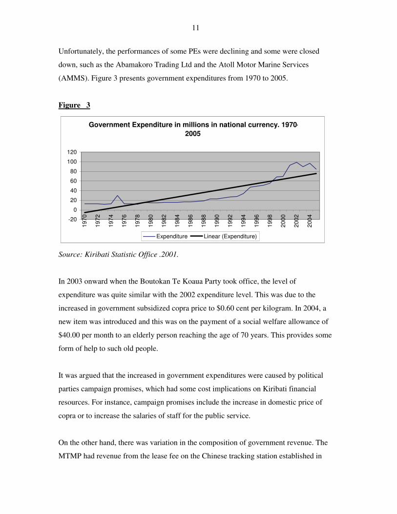
Unfortunately, the performances of some PEs were declining and some were closed

down, such as the Abamakoro Trading Ltd and the Atoll Motor Marine Services

(AMMS). Figure 3 presents government expenditures from 1970 to 2005.

Figure 3

Government Expenditure in millions in national currency. 1970-2005

-20

0

20

40

60

80

100

120

1970

1972

1974

1976

1978

1980

1982

1984

1986

1988

1990

1992

1994

1996

1998

2000

2002

2004

Expenditure Linear (Expenditure)

Source: Kiribati Statistic Office .2001.

In 2003 onward when the Boutokan Te Koaua Party took office, the level of

expenditure was quite similar with the 2002 expenditure level. This was due to the

increased in government subsidized copra price to $0.60 cent per kilogram. In 2004, a

new item was introduced and this was on the payment of a social welfare allowance of

$40.00 per month to an elderly person reaching the age of 70 years. This provides some

form of help to such old people.

It was argued that the increased in government expenditures were caused by political

parties campaign promises, which had some cost implications on Kiribati financial

resources. For instance, campaign promises include the increase in domestic price of

copra or to increase the salaries of staff for the public service.

On the other hand, there was variation in the composition of government revenue. The

MTMP had revenue from the lease fee on the Chinese tracking station established in

12

Tarawa, the green passports and the Norwegian Cruise Line operational fee and robust

revenue from the access fee. In July 2003, the BTKP got lid off with the green passport

and the lease fee from the Chinese tracking, as it had established diplomatic ties with

Taiwan, which becomes one of the major aid donors to the country. Also, the revenue

from the access fee was falling due to weather variation affecting the location of tuna

species. Consequently, the drawdown from the interest earned from the RERF to

balance government budget would be an alternative. Figure 4 below reflects the pattern

or regular composition of government major sources of revenue in 2005.

Figure 4.

PATTERN AND COMPOSITION OF MAJOR GOVERNMENT REVENUES IN MILLIONS IN NATIONAL CURRENCY: 2005.

Comp.tax5%

person.tax7%

fish. Licen33%

imp.duty24%

others5%

RERF26%

Comp.tax person.tax fish. Licen imp.duty others RERF

Source: Government of Kiribati (2004) – 2005 Budget.

The access fee (fishing license), the RERF and the import duty were the major sources

of revenues contributing to 35 percent, 27 percent and 24 percent respectively of

government total revenue in 2005, similar with previous years (Government of Kiribati

budget 2004 and 2005). One should note that only 5 percent of the total revenue was

acquired from company tax, a reflective of the underdevelopment of the private sector.

13

3.2. Gross Domestic Product (GDP) with its Average Growth Rates and Inflation

Government expenditure formed part of the GDP. There was a high GDP during the

colonial administration with a peak of $92 million in 1975 and dramatically fell to $36

million in 1980 caused by the cessation of phosphate mining, which had great adverse

effects to Tabai’s government (NPP) in terms of insufficient government’s revenues for

recurrent and development expenditure purposes. More expansionary policies were

experienced during the MTMP’s terms in office from 1994 to 2002. For instance, the

GDP level was increased from $54 million to $98 million for 1994 and 2002

respectively.

Government current expenditure was very large in relation to the overall economic

activity, accounting to 90 percent of GDP at factor cost in 1995, due to high level of

overseas earnings (Ministry of Finance and Economic Planning. 1997). The level of

expenditure was exactly the same in 2002, given a high support price to copra and a

pension welfare allowance.

The growth rate of GDP for Kiribati was fluctuated. After independence in 1980 it

recorded a poor growth due to cessation of phosphate mining, a major export item, and

gradually recovered in the late 1980s at low rate. In 1993 it stood at 1.7 percent, 1.6

percent in 2000 and in 2002 it recorded 0.9 per cent. In 2004, it had improved to 1.4%.

The variation in the annual average GDP growth rate was caused by the fluctuations in

the production sectors of the economy such as the revenue from the fishing licenses,

earnings from export of copra and seaweed, fluctuation in government revenues and

expenditures and business activities.

Inflation is quite low in the country however it is subjected to external forces

particularly from major import sources such as Australia, Fiji, New Zealand and other

international markets. For instance, the recorded inflation was averaged at 2 percent in

2003-04. (Kiribati national development strategy: 2003-2007). The increased in world

oil price would also indirectly increase domestic prices. Government’s imposition of

14

the price control on some major consumable imported foods and other commodity

items also assist to suppress inflation domestically.

3.3. Trade Liberalization

Global integration in terms of trade liberalization dominates much of the World Trade

Organization’s (WTO) agenda in the 21st century. 2 It is designed to eliminate trade

barriers (custom duty etc) globally as a foundation for free trade. The issue has

undoubtedly emerged following the success of regional trading blocks such as free

trade agreements between the Central American countries, the Dominican Republic,

and the United States (CAFTA-DR) and so forth. Also the Pacific Island Countries

Trade Agreement (PICTA) enters into force after six countries have ratified it.

The PICs together with Australia and New Zealand, have also signed the Pacific

Agreements on Closer Economic Relations (PACER), which is an umbrella agreement

for the PICTA. PACER is not fostering freer trade between PICs and Australia and

New Zealand. Wadan (2004) stated that it was a reactive and essentially defensive

agreement, protecting Australia and NZ interest in the PICs markets. For instance, if

any PICs proceed with formal negotiation with other developed countries, then they

should also have similar negotiation with Australia and NZ.

While the PICTA and PACER are already binding on those PICs signing and ratifying

it, the Cotonou Agreement on trade aspects are in the process of negotiation between

PICs with the European Union (EU), under the Economic Partnership Agreements

(EPAs), expected to come into effect after 2007. This means that PICs will try to make

agreements that will satisfy Australia and NZ as well as the EU countries (ibid).

2 Global integration is a widening, deepening and speeding up of interconnectedness in all aspects of contemporary social life in our case here is on economic activities. Economic globalization means the greater global connectedness of economic activities, through transnational trade, capital flows and migration. – see Glossary @ http://ucatlas.ucsc.edu/glossary.html�

15

Is Kiribati benefited from free trade? The important issue that Kiribati is encountering

now is how to substitute the loss of revenue from custom duties, which renders around

$10 million dollars annually into the economy or about 10% of GDP in 2002, if free

trade incorporated fully into the PICTA. Other forms of taxes such as the value added

tax for instance is being considered as an alternative. Is this going to increase the cost

of living and directly affecting the poor? Major arguments also suggest that the benefits

from free trade outweigh cost in Kiribati, considering its dependency on import (it is

normally in trade deficit), poor resource endowment and lack of investment in capital-

intensive manufacturing industries. Also one should note that if the VAT is imposed,

domestic price would also be increased on selected items.

Producers from the developed countries would also benefit from free trade. They can

now access other markets for their products, which assist to maintain or increase their

domestic employment and income.

3.4. Gross Domestic Product Per Capita and Employment

Given the low productive and absorptive capacity of Kiribati’s economy due to the

underdevelopment of the private sector, the adverse effect of the increasing population

on the GDP per capita is greatly felt. It is measured in the United States currency in

order to be able to compare with other countries. In 2000 to 2004, the GDP per capita

for Kiribati rose from US$560 to US$800 respectively, due mainly from the increased

in government expenditures, while as in 1974 coincidence with the high export earnings

from phosphate and moderate increase in population, the per capita GDP reached

$1,200. Also, after independence in 1980 there was a dramatic fall in per capita GDP

recording US$500 and reached 300 in 1986 the lowest on record, due mainly to the

cessation of phosphate mining. Figure 5 below shows the graph for GDP per capita.

16

Figure 5.

GDP per capita

0

200

400

600

800

1000

1200

1400

1970

1972

1974

1976

1978

1980

1982

1984

1986

1988

1990

1992

1994

1996

1998

2000

2002

2004

GDP per capita

Source: United Nations Statistic Division (2006)

The trend in employment varies. Employment has been increased since 1985 totaling

4,635 and 7,053 in 1994 (refer to figure 6), but these figures are only minimal

considering the increasing young active labour force available annually. Government

and its public enterprises are the main providers of employment accommodating 77%

of the total employees, while the private sector (consists mainly of churches, private

business, foreign companies and embassies and regional organization) rendered 23%

(MFEP.1997). In 1995 and 1999 Government accommodated 6,800 and 8,600

respectively, which accounted to 55% of the total employed workforce. Another 22%

was employed by public enterprises and 23% by private businesses (National

development strategies.2000-2003). In 2000 the public sector had employed 9,200

people (Toatu. 2004). It is also estimated that only 450-500 jobs become available for

1,700 to 2000 school leavers annually (ADB.2002).

Given that situation, it is significant that every government must diversify income -

generating activities for the rural people and encouragement of the private sector

development, in order to provide employment opportunities and income.

17

Figure 6.

Number of paid employees

0

1,000

2,000

3,000

4,000

5,000

6,000

7,0008,000

1985 1986 1987 1988 1989 1990 1991 1992 1993 1994

In t

ho

usa

nd

s

Number of employees

Source: Ministry of Finance and Economic Planning (1997).

4. Major Foreign Exchange Earnings

4.1. Fishing Access Fee

Given the prevailing very small-scale commercial tuna fishery sector (without canning

factory) in Kiribati, it does not gain much from the export of raw tuna to overseas

markets. However, its revenue from the access fee provides some financial means but at

a consistent low level and subject to short run fluctuations from distance water fishing

nations (DWFNs) economies.

The weather pattern is also affecting the movement of the tuna species and a major

factor to determine the revenue from the access fee. For instance, there was a drop in

the catch in 1994, which coincided with a strong La Ninã, followed by a strong El Ninõ

in 1995 when the tuna stock returned to a high level in Kiribati but failed to return to

the previous level in Fiji (Aaheim and Sygna.2001). After 1996 there was a big increase

in access fee received amounting to $40 million in 1998 and fell in 1999 to 2000 at

$31.5 million. The highest access fee revenue recorded was $46 million in 2001 or

about 40 percent of GDP ( ADB.2002).

18

The fluctuation of revenue from access fee is a major national issue. For example,

Kiribati parliamentarians during their parliamentary budget session in 2004 debated on

the reason for the fall in revenue from access fees. It was clarified that the negative

effect of climate change (La Nina) was the responsible factor.

This unstable revenue creates some problem. How can they balance the recurrent

budget when the revenue side continues to fluctuate or fall? Duncan (2004) argued that

it would be extraordinarily difficult to have good fiscal management when the revenue

side of the budget was so unstable. Figure 7 presents the revenue from the access fee.

Figure 7.

Ac c e ss Fe e R e v e nue f or K i r i ba t i

0

5

10

15

20

25

30

35

40

45

50

1979 1980 1981 1982 1983 1984 1985 1986 1987 1988 1989 1990 1991 1992 1993 1994 1995 1996 1997 1998 1999 2000 2001

Ye a r s

($ M

illio

ns)

Source: ADB (2002): Government of Kiribati National Development Plan 1983-1986: Statistic Office.2001. Government Finance Statistic (GFS) 1985-2000;

Given the fluctuation and low level of access fee received by Kiribati, it may consider

adopting a joint venture with one or more of the DWFNs in order to earn bigger share

from its EEZ and it is quite cheaper as they share the cost depending on their

agreement.

19

Tuna farming that is, to keep tuna species in fence in the lagoon, just like milkfish

ponds, is also significant considering Kiribati numerous lagoons in the outer islands.

The advantage for this is that, it does not require fishing vessels.

4.2. Revenue Equalization Reserve Fund (RERF).

The RERF is really the backbone of the Kiribati’s economy. It is normally used

annually to balance government’s budget. Obviously, there is a consistent increase in

the real value of the RERF reaching A$658 million in 2001 (ADB.2002). The draw

downs of the RERF has covered the current account deficit, but this can lead to

apprehension that the RERF’s value can be entering a long-term decline. Not only that,

but it is also vulnerable to short run fluctuations from major international economies

and financial markets. Figure 8 shows the growth in the RERF real value from 1985-

2001.

Figure 8.

Growth in RERF real value in A$ millions, 1985-2001

0

100,000200,000

300,000400,000

500,000600,000

700,000

1985

1986

1987

1988

1989

1990

1991

1992

1993

1994

1995

1996

1997

1998

1999

2000

2001

RERF value

Source: Kiribati Statistic Office (2001).

Kohn (2005) stated that no financial system that was efficient and flexible was

likely to be completely immune from episodes of financial instability from time

20

to time, and policymakers would be forced to make judgments about the costs

and benefits of alternative responses with very incomplete information.

The open market operations should be used, as a first resource to staving off

adverse economic effect of financial instability and to make sure aggregate

liquidity is adequate. Adequate liquidity has two aspects: First, we must meet any

extra demands for liquidity that might arise from a flight to safety; if they are not

satisfied, these extra demands will tighten financial markets at exactly the wrong

moment. This was an important consideration after the stock market crash of

1987, when demand for liquid deposits raised reserve demand; and again after

9/11 commonly known as the destruction to the world trade center, when the

destruction of buildings and communication lines impeded the flow of credit and

liquidity (ibid). Second, weighting the stance of monetary policy on the

adjustment to counteract the effects on the economy of tighter credit supplies and

other consequences of financial instability is worth considering. Rey and Martin

(2002) also pointed out that emerging markets were more prone to financial

crashes simply because they had a lower income level and not because of the

existence of market failures (moral hazard or credit constraints), bad monetary

policies or exchange rate regimes. The chain reaction resulted from such

financial instability, could assist to explain why there were major losses to

Kiribati’s RERF real value in some years.

The diversification of the RERF investment in various currencies under different fund

managers is a good measure to encourage competition and also to monitor performance

of financial markets. This is vital for the management and development of the reserve

fund. It is worth considering that such fund managers invest the reserve fund in

currencies stronger than the national currency (Kiribati uses the Australian currency).

On the other hand, this arrangement may not be working if such fund managers

work closely, which can be against the purpose of this arrangement where they

are required to work independently.

21

Given the economic significant of the RERF, the vital and priority requirement to be

implemented by the Ministry of Finance is to monitor and manage the fund properly in

order to have sustainability in its real value for future generations.

4.3. Remittances

Employment opportunities overseas or labour mobility are the sources of remittance.

Borovnik (2005) revealed that in 1999 the total number of seafarers registered with the South

Pacific Marine Services was 1366 and 569 registered with the Kiribati Fisheries Services.

Also, seafarers’ remittances in Kiribati consisted of 57 per cent remitted to wives spent on

basic needs, 30 per cent saved for investment and 13 per cent spent on school fees. At the

social level, remittances have added to family incomes and boosted private consumption. At

the national economic level, remittances have reduced, in some cases substantially, the

current account deficit of many developing countries, boost imports and spur growth,

increase a country’s international credit worthiness and lead to lower borrowing cost (see

ESCAP (2006); Walker and Nicholson and Matteo and Francesco (2005); Caroline and

Nikola (2005)). In 1979 the amount of remittance was $1.4 million and increased to $7.3

million in 1993. On average the contribution of remittances to GDP was 15 percent for

1996-2000, an increase from 7.2 percent as earlier reported by McGall (1992).

Given the economic important of remittance, Kiribati should maintain its quality seafarers

through supporting its marine training institutions’ development and to provide incentives

and to establish a good relation with the recruiting agencies based in the country, for the long

term sustainability of the seafarers’ employment and the remittance.

4.4. Official Development Assistance (ODA) or Foreign Aid.

It was noted that aid was frequently used to maintain or extend the strategic interests of

the major powers. However, some aid donors had considered the interest of the

recipient countries as well. For example, Japan, Australia and New Zealand and so

22

forth, take national interest as well as recipient country needs into account in allocating

their aid.

However, the purpose of ODA remains, for most donors, the alleviation of poverty in

developing countries through the promotion of economic and social development.

Kiribati for instance had already received a total of US$593 million since 1970

(Hughes.2003). The major sources of foreign aid are mainly from bilateral and

multilateral. For example the Public sector, which dominates the economy, relies on aid

averaging 27 percent of GDP over the 1996-2000 periods. The issue is that where does

this huge aid pour on? This is due to the fact that the level of development in Kiribati

remains low. However, Kiribati will endlessly require aid in the long term, but it is

important that aid donors will consider providing aid into productive investment.

4.5. Gross National Income Per Capita.

Kiribati’s gross national income per capita varies. For example, it had been in the

upward trend from 1970 reaching US$1,600 in 1974 with a major source of earning

was from the export of phosphate including low population. Figure 9 presents the

growth in per capita gross national income from 1970 to 2004.

Figure 9.

GNI per capita 1970-2004

0

200

400600

800

1000

12001400

1600

1800

1970

1972

1974

1976

1978

1980

1982

1984

1986

1988

1990

1992

1994

1996

1998

2000

2002

2004

GNI per capita

Source: United Nations Statistic Division (2006).

23

Since late in the 1970s, more foreign exchange earnings were acquired mainly from aid,

access fee, the RERF and remittances. They really contribute to GNI per capita. For

example, the gross national income per capita stood at US$1,100 in 1997 and further

increased to US$1,500 in 2004, but fell in 2006 to US$1,390.00 (World Bank.2006).

5. Conclusion

Kiribati’s foreign exchange earnings from the access fee, foreign aid, remittances and

the draw down from the RERF and trade are important for the development and

sustainability of Kiribati’s economy. There is a potential of deriving revenue from the

marine resource, given its huge EEZ, but currently there is no real investment in this

sector. Foreign aid is considered imperative given Kiribati’s financial constraints.

Foreign aid will be required in the long run, however, it is very important that aid must

create opportunities to contribute to productive investment rather than consumption. Its

increasing population is also a burden, as it requires more budget to cater for their

welfare. Unemployment is also a problem, thus labour mobility may be beneficial due

to weak absorptive capacity of the economy. The remittance from seafarers is important

to the families for their living and the economy at large. The RERF on the other hand, a

source of funding for the recurrent and development budgets must be managed properly

for the betterment of future generations. Although Kiribati may rely on foreign

exchange earnings, such earnings are vulnerable to short run fluctuations from partner

economies. Effort should also focus on the sustainability of government’s expenditures

given its limited financial resources. Trade liberalization may be beneficial to Kiribati,

but this will eliminate revenue derived from the custom duty. Therefore, Kiribati must

weigh carefully the positive and negative effects of free trade. Developments of the

coconut and seaweed industries for domestic and overseas markets are essential. The

concept of having import substitution industries (a foundation for the export led growth

concept) may be worth considering in order to lower the high import bill for Kiribati

and in the longer term can be engaged in the export led growth. Reducing barriers to

24

trade, investment, and marine development, environmental management and investing

in human resources development could foster opportunities for development.

25

3. THEORIES OF ECONOMIC GROWTH 1. Introduction

Why are we so concerned with economic growth? Why are some countries wealthier

than the others? Why do we have the so-called the more developed and Less developed

countries? These questions cannot be satisfactorily answered without a clear

understanding of the theories of economic growth. This chapter, therefore, briefly

examines these theories and is organized as follows. Section 2 surveys growth models

such as the Harrod Domar and the Robert Solow (1957) model and the usefulness of the

growth accounting. Section 3 examines the significance of the model to the Small

Pacific Island Countries, also known as the MIRAB (migration and remittances, aid-

bureaucrat) economies and a re-look at the MIRAB model. Section 4 concludes.

2. Economic Growth Theories

2.1. A brief look at Harrod Domar Model

The Harrod-Domar model observed that the rate of economic growth would depend on

the growth of capital, and on the proportion of income saved and invested. In other

words, the rate of growth of an economy can only be increased when we increase

investment (capital) and the saving rate to finance higher investment.

Furthermore, it stressed that investment would be "warranted" (that is, justified or

reasonable) only if the businessmen could expect that it would be sufficiently

profitable. Therefore, it reflects the fact that the rate of growth, which in this case is

warranted, is constrained by businessmen's expectations of profits.

26

The model states that technology through (marginal) capital-output ratio (�k / �y) is

fixed. The Harrod-Domar’s specification is as follows:

�lnYt = s / g (1)

where �lnYt = the rate of growth of output, s = saving rate and g = capital to output

ratio.

The question that we may ask: Is this model useful for economic policies in the real

world? Based on its specification, it may suit the high-per capita income countries such

as the United States, Japan and so forth because they can increase their saving rate to

finance higher investment. However, it is hard to increase the saving/investment rate in

the developing countries where per capita incomes are low.

2.2. The Solow model

The Solow model (1956) extended the Harrod-Domar model by incorporating these

assumptions: adding labour as a factor of production; the returns from labour and

capital are diminishing separately and both have constant returns to scale; introduce

technical progress variable as exogenous and dissimilar from capital and labour. Also,

the capital-output and capital-labor ratios are not fixed as they are in the Harrod-Domar

model. These refinements allow increasing capital intensity1 to be distinguished from

technological innovation.

1 see Exogenous growth model-"http://en.wikipedia.org/wiki/Exogenous_growth_moel"

27

2.2.1. Specification of the Solow Model

2.2.1.1. Defining Capital Value

Let us start first with the capital stock (K), one of the inputs in the Solow model as

conveyed in the Cobb-Douglas production function in equation 2.

( , , )Y F K L A= (2)

However, one should note that the use of tools and machinery make labor more

effective, rising capital intensity or capital deepening thus pushes up the productivity of

labor. A society that is more capital intensive tends to have a higher standard of living

over the long run than one with low capital intensity. However, capital depreciates

depending on the quality and life span of machineries. In other words, we can say that

the capital stock (�K) can be acquired from gross investment less depreciation:

K s Y d KΔ = × − × (3)

Where Y is output and s represents the proportion of income we save and invest i.e,

assuming all savings are to be invested and d is depreciation rate.

We can arrange equation 3 in order to get the proportional change in K. Dividing both

sides of the equation by K can do this;

/ / /K K s Y K d K KΔ = × − × (4)

For illustration, assume Y = 1020, s = 0.25, K = 2000 and d = 0.05,

So the change in capital KΔ = .25 x 1020 – 0.05 x 2000 = 155. In proportional terms,

( )/K KΔ = (155/2000) � 7.7%.

28

Let us look at the balanced growth path (BGP), as it is important in the growth models.

Assuming that the economy is on a BGP, the proportional change in K is zero as

illustrated here 2.

/ 0 /K K s Y K dΔ = = × −

/d s Y K= ×

* ( ) /K s Y d= × (5)

The K* is the capital when the economy is on its BGP. The assumption in equation 5

implicitly reflects the non-existence of technical progress and no growth in labour

force. However, the opposite will happen, that is the BGP value of K* changes, if there

is technical progress and growth of the labour force.

2.2.1.2. Defining Value and Growth Output

One important thing, which is an objective, is based on the assumption that when the

economy is on BGP, we must find the value of its output and its growth. The value of

capital (K*) has already been defined in equation 5 when the economy is on its BGP.

The value of output on the other hand, when the economy is on BGP can be obtained

using a simple dominant device Cobb-Douglas production function (equation 6) with

constant returns and non existence of technical progress and growth in employment,

that is, these rates of growth are zero.

1Y K Lα α−= (6)

Since we have already found the value of K*, we can use it to substitute into equation

7. This is illustrated below,

2 Professor Bill Rao of the University of the South Pacific provided useful lecture notes on EC401 in 2006 for the application of the Solow model, which they are also referred to here.

29

1* [ * / ]Y sY d Lα α−=

1* ( *) ( / )Y Y s d Lα α α−=

(1 )* ( / ) 1Y s d Lα α α− = −

/(1 )* ( / )Y s d Lα α−= (7)

Based on equation 7, we can find the proportional changes in output, but remember that

s, d and L are constants. Therefore, (7) implies that:

* / * 0Y YΔ = (8)

The conclusion here states that, when the economy is in BGP, the capital stock will

remain constant.

2.2.1.3. Growth in Labour Force and Technical Progress

We assume now that employment and technical progress grow at the exogenous rates of

n and g. Using the per worker capital stock ( / )k K L≡ we get

/ / / /k k K K L L K K nΔ = Δ − Δ = Δ − (9)

where n is an exogenously given rate of growth of employment.

Since we have known the value or expression of /K KΔ , we can use it also to

formulate the growth in employment and technological progress

/ [ / ] , / / / / ( ) / ( )k k sY K d n or k k sY L K L d n sy k d nΔ = − − Δ = − + = − − (10)

We can also use the per worker capital stock deflated by the stock of knowledge.

[ ]/ /K K sY K d n gΔ = − − −

( ) ( )/ / / /sY LA K LA d n g s y k d n g= − + + = − + + (11)

30

where g, is exogenously given rate of growth of technology. This is important in

finding the BGP values of output and its rate of growth.

When the economy is on BGP, / 0k kΔ = , so we have this

( )/ 0s y k d n g− + + = (12)

The BGP value of k is *k = /s y d n g+ + (13)

We must then substitute k into the production function, using the Harrod neutral

technical progress as shown below.

( )1

Y K LAαα −

=

Dividing both side by LA

( )/ /Y LA K LAα

=

y kα

= (14)

Substituting equation 13 into 14 gives equation 15. Equation 15 is a growth rate of *y .

( )/y s y d n gα

= + +

[ ]/(1 )

* /( )y s d n gα α−

= + + (15)

Our next objective is to get the growth rate in per worker income y reflected in the

following equations.

[ ]/1

* /( )y s d n g Aα α−

= + + × (16)

[ ] [ ]ln * /(1 ln ( / ) lny s d n g Aα α= − + + +

ln * 0 lny A gΔ = + Δ = (17)

31

Equation 17 is important as it shows that when the economy is on a BGP, per worker

income will grow at the rate of technical progress (g). If g = 0 then per worker income

will not grow. We can say here that the growth in per worker income is depended on

the rate of technical progress. The Solow model implies that the economy converges to

a BGP because each variable is growing at a constant rate. The BGP implies that the

growth rate of output per worker is determined by the rate of technical progress.

Therefore, it would be valuable to know (a) what the value of the rate of growth of

technical progress is for each country; (b) what factors determine the size of this rate of

growth of technical progress and (c) why it may differ from country to country.

Needless to say answers to the questions are useful to develop growth policies.

However, Solow (1956) has no answers to these questions, except to show that while a

country’s growth rate may vary from year to year, in the long run, when an economy

reaches its equilibrium growth path, its per worker income grows only if there is a

positive technical progress. Subsequently, Solow (1957) showed how to estimate the

rate of growth of technical progress by using the identity implied by the production

function. This is known as growth accounting.

2.2.1.4. Usefulness of Growth Accounting

Durlauf and Kourtellos and Tan (2005) stressed that the aim of growth accounting was

to estimate the relative portions of variation in cross-country output per worker, or

growth, which could be assigned to variation in factor accumulation rates and that

which accrues to total factor productivity (TFP).

It can be used to determine the relative importance of factor accumulation to growth,

even though we do not know what determines the Solow residual. However, the results

from growth accounting exercises are useful for designing growth policies (see also

Herendorf and Vanlentinyi (2005), Bosworth and Collins and Chen (1995), Pinheiro

and Serven and Thomas (2001)).

32

Musso and Westermann (2005) also provided concrete fact about growth accounting,

stating that it does not aim to explain the fundamental underlying forces, such as

preferences, institutions and economic policies, that drive the evolution of supply-side

factors, nor does it take into account the linkages between developments in these

factors. This is a useful contribution towards the understanding of growth accounting in

terms of longer term growth process. It is a useful complement to model based

approaches to estimating and assessing potential output, which is true for any

production function based approach.

Senhadji (2000) stressed also that growth accounting framework had been used

worldwide to examine the source of cross-country differences in total factor

productivity (TFP) level. He highlighted that this exercise has been conducted for 88

countries for 1960 – 1994.

Several growth accounting exercises results had useful results. Solow (1956) argued

that the residual and not factor accumulation accounted for the bulk of output growth in

the US. Denison (1962), found out that 60% of the growth in the advanced countries

was due to total factor productivity or technical progress. Therefore, this method of

estimating technical progress is known as the residual method and often the residual

attributed to technical progress is known as the Solow residual.

Some economists like Caselli and Rao call this Solow residual as a measure of our

ignorance of the determinants of the growth rate. The reason for this is that, the Solow

model does not offer any explanation of what factors e.g. like education, health,

expenditure on research and development etc, determine this residual. Often in the

empirical works it is assumed that it is a constant and can be estimated as the

coefficient of time trend. For example if the production function is written as Y= A0 egt

Kα L(1-α), where A0 is the initial stock of knowledge, then it is possible to estimate `g’,

say with OLS. However, this does not answer what factors determine `g’. All that this

implies is whatever these determinants are, they are highly trended. Such an answer

33

does not help to develop growth policies. Therefore, Caselli and Rao are justified in

calling the Solow residual as our measure of ignorance of the determinants of growth.

3. The MIRAB Economies and Growth model

3.1. What is the MIRAB?

The MIRAB is the acronyms for Migration, Remittances, Aid and Bureaucracy.

Bertram’s (1985) insights into the MIRAB model, by and large, is based on his

experiences of working in such countries, collecting and studying macroeconomic

statistics, which are considered to be the MIRAB economies stylised facts. He stressed

that there were five components of the MIRAB economies.

The first was migration. Appleyard and Stahl (1995), Doumenge (1991) and McCall

(1997) stressed that migration removed significant part of the workforce and

highlighted the number of people migrated from some Pacific Island Countries. For

instance, about 56,000 Cook Islanders migrated leaving only about 16,000 live in their

homeland. Also there were 10,000 Niueans in the world and only about 2,000 actual

live on Niue. The pattern of migration is a common feature of Polynesians, with lesser

extend to Micronesians, but not of the larger islands of Melanesia.

The second component of MIRAB is remittances and it is bound up intimately with

migration. These are payments in cash or kind sent by migrating relatives to their kin

back home, which and are used to finance local development, for local constructions

and for educational and other expenses of family. With Samoans and Tongans being so

widespread in the USA, Australia and New Zealand, this has led some researchers to

call this kind of activity "the trans-national corporation of kin". In Tonga, at the

national level, remittances are the major source of foreign exchange and accounted in

2002 for about 50 percent of GDP. Seventy-five percent of all Tongan households

report receiving remittances from overseas, making remittances the single most

widespread source of income in Tonga (see Small and Dixon.2004). In the same year,

34

Samoa received US$57 million, Fiji US$53 million, Kiribati US$6 million, Solomon

Islands US$15.9 million, Vanuatu US$30.6 million and Tuvalu US$4.9 million in

2001.

The third component of the MIRAB model is ODA, or "Official Development

Assistance", known also as Aid. Since the 1970s, a total of US$49,258 million aid

flows to the Pacific countries, which is equivalent to US$220 per capita.3

In order to administer the complexities of aid, a final component is added: a

Bureaucracy is erected to fulfill the requirements of accountability & the provision

"counterparts" for training (McCall.1997). Therefore, the MIRAB model shows the

direct inter-relationship between migration and remittances, as well as for aid and

bureaucracy.

3.1.1. A Re-Look at the MIRAB Model

As currently the case, the MIRAB economic model offers an explanation of the

evolution and operation of some tiny Pacific island economies. Proponents of the model

have argued that it describes an economic system that is durable and persistent, while

others have opposing views. Since we have much on the good side of the MIRAB

model, it is imperative to consider views against it. Treadgold (1999) argued that

Norfolk Island possessed strong MIRAB characteristics from the end of World War II

until the early 1960s, when the tourism-dominated economic growth erased these

characteristics, or at least reduced them to insignificance, thus the island has achieved a

sustained break-out from the MIRAB mould, but with some social costs incurred.

Boland and Dollery (2005) in their study on Tuvalu stated that the greatest volumes of

remittance are not from migrants but from a large number of seafarers.

3 see OECD the Development Assistance Committee, Development Co-operation Reports, 1971-2000, OECD Paris. Aid flows include official development assistance (including the concessional elements of loans) from OECD countries, multilateral organisations and Arab countries. Hughes (2003).

35

The fact of the source of remittance in Kiribati is also not well researched. Since 1970

up to 1990s, permanent migration was only minimal and their contributions in terms of

the remittance were also low as they migrated with their families. The large bulk of

remittances now are coming from seafarers working on SPMS and DWFNs fishing

vessels. However, since the early 2000s considering the increasing number of skilled

people and lack of employment opportunities at home, I-Kiribati are now migrated with

their families to overseas countries, notably to New Zealand, given a favourable NZ

policy of allowing Pacific countries with specific quotas for residence permit. This

means that it is doubtful whether they will remit some money to Kiribati or not,

because they are living with their families overseas. In essence, labour mobility seems

important to the MIRAB economies, given their low absorptive capacity for

employment.

However, one important question regarding the MIRAB is that: Is it sustainable in the

long run? It solely depends on overseas economies and if there is short-run fluctuation

in such economies, or diplomatic ties is not favourable, it will also likely affect the

remittances. In addition, such overseas countries in which the MIRAB depends on have

their own internal problems such as they have also high population and limited

employment opportunities. Moreover, there will be competition in the skilled labour

placement in the developed countries among the Pacific islands and the Asian

developing countries, which can cause the declining in remittance by some countries.

For example, in Kiribati the number of seafarers working overseas is encouraging due

to the quality of workmanship rendered. However, given the cheap labour force from

the pacific-rim developing Asian countries such as the Philippines can affect Kiribati’s

seafarers’ job and remittances. In actual fact, the best option for the MIRAB economies

is to develop their own economies for longer-term sustainability in terms of

employment and income.

3.2. Examining the relevancy of growth models

The Solow model really is imperative to the real world. It states that a sustained

increase in the investment ratio increases the growth rate only temporarily, based on the

36

fact that the ratio of capital to labour goes up but the marginal product of additional

units of capital decline, making the economy to move to the long term equilibrium level

of output. In the steady state, real GDP, capital and the workforce are growing at the

same rate, meaning that output and capital per worker are constant. The key argument

of the Neo-classical economists is that, to raise an economy’s long-term growth rate,

they need to increase the productivity of labour and capital. In other words, increase the

efficiency of the production processes. Given the fact that the level of development and

economic growth is differing between economies, such differences are attributed to the

differences in the rate of technological progress between these countries.

Despite the label that MIRAB conveys for Kiribati, may imply that Kiribati is a

technologically backward country with labour intensive technology. It may be noted

that these economies are currently adopting capital-intensive industries in the area of

manufacturing. For example, Kiribati has already established a copra mill; a biscuit and

some private owned bread-manufacturing units which use semi automatic machines.

Nonetheless, growth in the MIRAB economies is low due to the slow pace of private

sector development and lack of foreign direct investment.

There is more than one way of applying the Solow model to develop growth policies

for the developing countries, including the MIRAB countries. In other words, the

usefulness and applicability of the Solow model is not limited to the problems of the

developed countries.

Firstly, as pointed out in the previous section, it can be used for growth accounting to

determine the relative importance of factor accumulation to growth, even though we do

not know what determines the Solow residual. Determinants of the Solow residual

become important if the Solow residual is high. In many developing countries this

residual may not be high. For example, it is well known that Young (1994&1995) has

shown that factor accumulation is the dominant determinant of growth in the leading

East-Asian countries, although some overtly sensitive economists have challenged his

findings from these countries. If factor accumulation plays a dominant role in growth,

37

then increasing the investment ratio and growth of employment are necessary to

increase the growth rate.

The fact that technical progress is low in these countries is a secondary issue. It is true

that increase in factor accumulation does not have effect on the long run BGP growth

rate of an economy. Nevertheless, as we shall argue below, results from growth

accounting exercises are useful for designing growth policies.

Secondly, as Rao (2006) has shown that an increase in the investment ratio (`s’ in our

earlier equations) will boost the growth rate of an economy for couple of less than

decades. Generally the economy may take well over 50 years to reach its BGP. These

findings by Rao are based on the simulation results with the Sato (1999a) closed form

solution for the Solow model. Many economists have neglected and forgot the use of

this closed form solution for the short to medium term growth policies in the

developing countries. Furthermore, the high growth rates experienced by the East-

Asian countries through high rates of factor accumulation for decades supports Rao’s

simulation results. Therefore, the closed form solution for the Solow model can be used

to compute the dynamics of the growth rates, for given investment ratios or compute

the required dynamics of the investment ratio for given targets of the growth rate.

Thirdly, based on the results from some growth accounting exercises for Fiji, one may

expect that in small island countries like the Pacific Island countries, the size of the

Solow residual would be very low. For example, in Fiji, the Solow residual is small and

contributed less than 10% to the growth rate. When the production function for Fiji is

estimated, the rate of technical progress, proxied with the coefficient of time trend, was

hardly half a percent. 4

4 These results are based on the computer laboratory exercises set for EC401 (Advanced Macro Economics) at the University of the South Pacific, in 2006. The lectures were given by Prof. Rao and the lab-sessions were supervised by Mr. Rup Singh.

38

Although some, like the East-Asian economists, may feel disappointed with the low

contribution of technological progress to the growth rate, one may take a positive view

and get an idea about the scope for improvements in efficiency in the growth processes.

It is hard to improve a rate of technical progress of 2% to 4%, but not so hard to

improve from 0.5% to 1%. Whether these small island countries aspire for 1% or 2%

rate of technical progress and therefore a 1% or 2% long run BGP growth rate, it

should be realized that it is hard to increase this rate of growth of technology in one or

two decades. These improvements may need historical time units, especially given the

cultural factors of these countries, which were not influenced by the impact of an

industrial culture for long periods like the Western countries. These hurdles for

improving technological progress in the non-western industrialized countries are not

adequately recognized by many Western-minded economists.

The fact that the Solow residual is small is to be taken seriously by the development

economists and policy makers. That is, they should begin to think about what are the

long term policies, e.g., improving education, health and good governance practices etc,

that are necessary to maintain the current higher but temporary growth rates achieved

through higher investment rates. This way, there is no conflict between the medium and

long-term objectives and policies for growth and development. This is a more

appropriate approach.

One of the important steps for the fulfillment of such aforesaid vision is through the

establishment and provision of training institutions for the labour force. Kiribati for

example, has already established two big important training institutions such as the

Marine Training Center and Kiribati Fisheries Training Center. Overseas companies

such as the South Pacific Marine Services and the Japan Tuna are currently employing

healthy young men and women, after completing their course from such institutions. It

is estimated that about 2,000 seamen are working overseas on merchant and fishing

boats, and the amount remitted to Kiribati is around A$6 million annually, which is

about one third of household consumption expenditure in 2005 and 2004.

39

It can be eventually expensive if, for example, Kiribati invests in high level of

education to increase labour productivity, out of proportion to its needs. This is so,

because there are no opportunities to employ them at home and therefore they may

migrate to the neighboring advanced countries like Australia and New Zealand. They

may send money back home, which is useful for the families.

Although the quality of the labour force is a key for technical progress, one should not

lose sight of the needs of the economy while thinking about policies to increase

technical progress. It is true that research and development expenditure may have a

high impact on the growth rates of the USA, Germany and Japan. However, it is

unlikely that high R & D expenditures will have similar effects in Fiji or Kiribati, given

their small developing economies and small scale industries.

Another major problem with the MIRAB economies is that, the levels of school

attainment rates are high at the primary and secondary levels. Only a fraction proceeded

to higher institutions. Therefore, even though education, through human capital

formation may contribute by one third to the growth rate, such as in the MRW

estimates, in the MIRAB economies there is already sufficiently educated work force,

relative to their current needs. What they lack are investments in industries to absorb

the work force, perhaps after training for short periods, to learn the specific skills

required in the new factories.

4. CONCLUSION

Based on the fact in which the Solow model is formulated, it totally renders insightful

analysis of the real world open economies growth rates. We cannot know what the

differences in the growth rates in factors of production are, unless we apply the growth

accounting exercise. This device is useful as it can be used to determine the relative

importance of factor accumulation to growth, even though we do not know what

determines the Solow residual or total factor productivity. However, the results from

40

growth accounting exercises are useful for designing growth policies. It is estimated

that there is low percentage of the Solow residual in all of the MIRAB economies.

Rao (2006) based on his simulation results stresses that an increase in the investment

ratio (‘s’) will boost the growth rate of an economy for a couple decades or even more.

The high growth rates experienced by the East-Asian countries through high rates of

factor accumulation for decades support Rao’s findings.

Development economists and policy makers should begin to think about what are the

appropriate long-term policies for growth? For example, improving education, health

and good governance etc, that are imperative to maintain the current higher but

temporary growth rates achieved through higher investment rates.

Growth in the MIRAB economies has been characterized as poor. For example, in

Kiribati the economic growth is low due to the slow pace of private sector development

and lack of foreign direct investment with limited employment opportunities. Given the

increasing population, unemployment and poverty will prevail.

A key argument by the Neoclassical is that, to raise an economy’s long run growth rate,

they need to increase the productivity of labour and capital or increase the efficiency of

the production processes. Although this is a common approach, it has limited success in

Kiribati given the very small number of its manufacturing industries. The variation on

the level of development and economic growth between economies is attributed to the

differences in the rate of technological progress.

41

4. DATA 1. Introduction

Applied econometric work needs reliable data. National accounts aggregates are the

major sources of time series data. Unfortunately, it is a problem in Kiribati. Only few

time series data for macroeconomic variables are available locally. Therefore, data are

acquired from external source mainly from the United Nations Statistic Department

(UNSD) or have to be estimated provided they are not available from both sources.

The structure of this chapter is as follows: In section 2 provides definitions, data

sources, the trend analysis of variables and method to analyze data and concludes in

section 3.

2. Definitions, Data Sources, Trend Analysis of Variables and Method to

Analyze Data

2.1. Nominal and Real GDP

Gross Domestic Product (GDP) is the market value of all final goods and services

produced within a country during a given time period. In terms of measuring GDP,

there are two methods used. The first one is the Nominal GDP, which is the dollar

value of production at current-year prices. The second is the Real GDP calculated by

valuing all the productive activity within the country at a specific year's prices. Based

on data for instance, the real GDP in 1991 prices for Kiribati is $38,444,000. This real

GDP is an important variable where most economic analysts focus on as it shows the

underlying strength of an economy.

42

2.2. Real GDP growth rate

The average rate of growth of GDP from 1971-2005 was negative at only half a

percent. The highest growth rate was 0.56% in 1974 and the lowest was -0.57% in

1990. The reason was that, there was robust export earning from phosphate mining in

the early 1970s and ceased in 1979. In the 1980s copra and fish were the major export

items and the fishing access fee and the drawdown of the RERF were major foreign

exchange earnings contributing to government revenues. The high negative growth rate

in 1990 was related with the fall on consumption recording $49 million in 1990

compared with $51 million in 1989 and the fall on export earnings to $40 million in

1989 compared with only $8 million in 1990. The standard deviation was 0.18 implying

that the variation in the growth rate has been very high. Figure 1 conveys the growth

rate of the real GDP from 1971 to 2005, after adjusting the UNSD data (see procedure

in estimating capital).

Figure 1.

Real GDP Growth Rates

-1

-0.5

0

0.5

1

1970

1972

1974

1976

1978

1980

1982

1984

1986

1988

1990

1992

1994

1996

1998

2000

2002

2004

Years

Gro

wth

rat

es

DLY

Source: Author’s calculation from UNSD data.

We can breakdown the periods 1971 to 2005 into three components to see their average

growth rate and standard deviation. From 1971 to 1979, the average growth rate was

43

0.026 and its standard deviation was 0.235, inferring a high variation in the growth rate.

For the periods 1980 to 1990, the average growth rate was -0.053 and its standard

deviation was 0.259, meaning that there was also a high variation in the growth rate.

The trend on the growth rate from 1991 to 2005, have been quite stable with an average

growth rate of 0.0116. Its standard deviation was 0.075, implying that there was small

variation in the growth rate.

Further more during 1971 to 1989, while the average growth rate of GDP was about

1%, from 1990 to 2005 this positive growth has become negative. In this latter period

the average growth rate of GDP was -2.6%. However, if we exclude 1990, the average

growth of GDP from 1991 to 2005 was again positive and is about 1.2%. Therefore, it

might be necessary to leave 1990 data in our subsequent analysis or introduce a dummy

variable for 1990 to minimize a large one off decline in the rate of growth of real GDP.

Similarly, it might be also necessary to introduce another dummy for a one off high rate

of growth of GDP in 1974. It may be also noted that the variance of GDP growth has

declined from 0.19 during 1971-1989 to 0.075 during 1991-2005.

2.3. Estimating Capital

There are some problems with the UNSD data for Kiribati, although these data are

comprehensive.1 Firstly, the nominal and real values of the components of GDP are not

equal in the base year of 1991. In solving this problem, the implicit GDP deflator was

computed in the usual manner by deflating nominal GDP with the real GDP. Secondly,

this GDP deflator was used to deflate all the nominal values of the GDP components to

estimate their real values. Thirdly, the estimate of real GDP is computed by using the

usual GDP identity. The justification for this procedure is that estimates of the nominal

values of GDP and its components are likely to be more accurate than estimates of their

real values. This assumption is used subsequently to estimate the real capital stock with

the standard perpetual inventory method.

1 I acknowledge the comments by Professor Bill Rao on capital estimation.

44

Capital stock is estimated with the perpetual inventory method. The assumed initial

period value of capital stock in 1970 was 1.2 multiplied with the level of output and the

depreciation rate assumed at 4%. These assumptions are justified and consistent with

the assumption used by Collins and Bosworth (2003), who have estimated capital stock

in several developed and developing countries, although they have used higher capital-

output ratio of more than two for the developed countries to estimate the initial period

capital stock. In applying this procedure to Kiribati, the capital-output ratio turned out

to be implausibly high such as after 1988 it suddenly increased up to 13 in 1995.

Estimate of capital stock, with the original UNSD estimate of real GDP components

showed a modest, but nevertheless has significant increases in the capital-output ratio.

It reached a high value only in a few years but on the average it was about 3.7

compared to an average of 8.7 based on the estimates from our real values. We shall

later address this high estimate of capital-output ratio later in the thesis. Figure 2 shows

the capital-output ratio for Kiribati from 1970 to 2005.

Figure. 2

Capital-Output Ratio

0

2

4

6

8

10

1970

1972

1974

1976

1978

1980

1982

1984

1986

1988

1990

1992

1994

1996

1998

2000

2002

2004

Years

K/Y

Rat

io

K/Y

Source. Author’s calculation from UNSD data.

There seem to be two plausible reasons for the high capital output ratio for Kiribati.

Firstly, the data may be weak by UNSD mainly on the fixed investment figures.

45

Secondly, even if the UNSD’s investment figures are acceptable, the increase in capital

output ratio is basically related to the increase in investment on non-value added or

unproductive projects. In other words, such investment, mainly by aid donors and the

government through high government’s expenditure did not increase output. Some of

the investment expenditures are on infrastructure development, where expensive

machineries and equipments are purchased overseas, school development projects such

as on improvement on classrooms and curriculum materials and expatriates salaries etc,

social projects in the outer islands for strengthening capacity development such as on

construction of village permanent and public buildings, roads and seawalls. Also, in

1986, the Japanese government funded the construction of the biggest multi million

dollar permanent causeway linking Betio islet to the main island of Tarawa. Moreover,

in the early 1980s, Japan had also constructed the fish storage facilities and the port and

the British had constructed the jetty at the port. The Government of Kiribati on the

other hand spent about $9 million dollars on its new parliament complex constructed by

Dai Nippon construction in 1998, which completed in 2000 to coincide with the Pacific

Islands Forum meeting in Kiribati. We may say that these are unproductive

investments and mainly for infrastructure developments etc, and much of the funds may

have been wasted and/or paid to foreign experts as salaries, contracts and importation

of materials or equipments.

The report from the Statistic office of Kiribati (2001) stated, on similar line that the

significant portion of capital spending was on buildings and civil constructions such as

roads and port construction, which reached a total expenditure of $6.8 million in 2000.

Since this Office had pointed out that they did not get data on projects actual spending

and cost breakdown, the presumption was that the UNSD data might have been based

on some estimates and aid data.

2.4. Real Capital Growth Rate

The average growth rate of real capital for 1971 to 2005 was 0.047 with a standard

deviation of 0.032. This showed that there was a high variation in the growth rates. The

46

highest growth rate for capital was in 1979 of 0.13, 1992 with 0.12 and 2001 recording

0.085. The reasons for the high growth rates were as follows. Fixed investment in 1978

was only $93 million compared with $105 million in 1979. The same pattern occurred

in in the 1991 and the 1992 level. The high growth rate for 2001 was also based on the

high investment in 2001 recording $319 million, while as in 2000 it recorded $293

million. The lowest growth rates were in 1981 and 1982 recording -0.01 and -0.02

respectively, because the amount of investment in 1981 was $163,000.00 and in 1982

fell to $114 million. Figure 3 reflects the growth rate in capital from 1971 to 2005.

Figure 3.

Growth Rate in Capital

-0.020

0.020.040.060.080.1

0.120.14

1970

1972

1974

1976

1978

1980

1982

1984

1986

1988

1990

1992

1994

1996

1998

2000

2002

2004

Years

Gro

wth

rat

e

DLK

Source: Author’s calculation from UNSD data.

2.5. Labour Force.

Labour represents active labour force in formal employment in the public and the

private sectors and the active work force in the rural production sector. The UNSD

does not provide estimate for employment. Therefore, in estimating Labour, local

sources from the Statistic office and the taxation office were used.

47

Active labour falls within the age group of 24-49 years of age or 36% of the total

population. This specified percentage figure is used to estimate active labour force from

1970 to 2005. Figure 4 shows the growth rate in labour from 1970 to 2005.

Figure 4.

Growth in Labour

00.005

0.010.015

0.020.025

0.03

1970

1972

1974

1976

1978

1980

1982

1984

1986

1988

1990

1992

1994

1996

1998

2000

2002

2004

Years

Gro

wth

rat

es

DLL

Source: Calculated by author from UNSD data

The mean growth rate of Labour stands at 0.23 with a standard deviation of 0.005,

meaning that there is also variation in the growth rates. There was a consistent increase

in mployment from 1972 until 1987 as shown from their growth rates and fell from

1988 to 1993 due to the big increase in employment and quite stabilized until 2003.

Also, there was a big drop in the growth rate in 2004 and a gradual fall as well in 2005

reaching 0.006. The fluctuation was related with the fact that Kiribati at times

experiences high increase in employment from year to year based on the economic

activity of the country, as well as the drop in employment relating to economic short

run fluctuation.

48

2.6. Official Development Assistance or AID

Aid figures for 1970 to 1979 are estimated, due to their unavailability in local and

external sources. The other source of data is from the Statistic Office in the

Government Finance Statistic ( 2001).

The mean growth rate for aid from 1970 to 2005 stood at 0.124 with a standard

deviation of 0.28, implying that there was a big variation in the growth rate. The big

increase in aid was in 1976 coinciding with the self-government of the Gilbert and

Ellice Islands Colony, where foreign governments provided some aid such as the

British, Australia, New Zealand and Japan. Also since independence in 1979, the

inflow of aid was increasing, but at times dropped due to some other commitment by

such aid donors, inferring that aid donors have specific interest, hence it was unreliable.

For example, funding of project by aid donors would be ceased once they were

completed. In 1992 the total amount of ODA reached $33 million due mainly from the

implementation of numerous government projects on the outer islands such as seawall,

causeways and so forth. Figure 5 shows the growth in the real ODA flow to Kiribati

from 1970 to 2005 in national currency.

Figure 5.

Real Growth in Aid

-1

0

1

1970

1972

1974

1976

1978

1980

1982

1984

1986

1988

1990

1992

1994

1996

1998

2000

2002

2004

Years

Gro

wth

rat

es

DLA

Source: Calculated by Author from Statistic Office (Government finance statistic),

2001.

49

From 2000 until 2005, there was stability in the growth rate, given that some aid donors

such as Australia, New Zealand for instance, had specific annual aid programmes to

Kiribat,.including the European Union and Japan, meaning that the flow of aid was

more reliable by such aid donors. Kiribati had already received a total of US$593

million of aid since 1970 with an average annual aid flow per capita since 1970 of $217

millions (Hughes.2003).

2.7. Remittance

Remittance is one of the major sources of foreign exchange earnings for Kiribati. There

were small amounts of remittances in the early 1970s. This was due mainly to the first

operation of the marine training school (MTS) in the late 1960s. A further increase in

the remittance was experienced in subsequent years following the on-going passing out,

continue intake of trainees of the MTS known now as the Marine Training Center

(MTC), and the on going employment of seafarers overseas. The source of data for

remittance in Kiribati is from the South Pacific Marine Services, the Kiribati Fisheries

Services and Borovnik (2005).

The average growth rate of remittances was 0.19 with a standard deviation of 0.29.

Again there was also a big variation in the growth rate. The remittance in 1976 stood at

approximately hundred thousand dollars, while as in 1975 it was only eighty thousand

dollars. In 1979 and 1980 the figure remained at $1.5 million, but increased in 1981 to

$1.7 million. In the early 1990s, the amounts were increasing, recording $6 million in

1990, $11 million in 1998 with a peak of $14 million in 2003. These increases reflect

the increasing number of seafarers working on overseas vessels. The inclusion of

fishermen’s remittances working on Japanese tuna fishing vessels and seamen on the

Norwegian cruise liners were also factors responsible for the increased inflow of

remittances to Kiribati. Figure 6 below shows seafarers’ remittances for Kiribati from

1970 to 2005.

50

Figure 6.

Growth rate of Real Remittances

-0.5

0

0.5

1

1.5

1970

1972

1974

1976

1978

1980

1982

1984

1986

1988

1990

1992

1994

1996

1998

2000

2002

2004

Years

Gro

wth

rat

es

DLRR

Sources: Calculated by author from SPMS data 1999 unpublished, KFS data 2004 unpublished, Borovnik (2005).

Obviously, the fluctuation in the growth rates show the fluctuation in the amount of

remittances sent back to Kiribati. One major reason was that, the employment of I-

Kiribati seafarers depended on the availability of ships and demand from such overseas

based employing agencies, as the number and quality of seafarers was adequate,

consistent and maintained. Also, the foreign exchange rate had some effects in the

amount of remittances received, given that seafarers were paid in the United States

currency, which must be converted to the Australian dollar or national currency.

2.8. Real Export Earnings from Copra

The mean growth rate for the real earning from the export of copra stood at –0.0008

with a standard deviation of 0.88, implying a more consistent growth rate. There were

higher exports earnings recorded in 1974 ($4.8 millions), 1984 ($7 m), 1988 ($4.2m),

1992 (4.3 m), 1995 ($6.4 m) and in 1999 with $8.7 millions and gradually fell from

2000 onward. The export earnings also showed a big drop as reflected in the growth

rate and vice versa. One major factor was the fluctuation or instability in the world

price of copra, exchange rate and volume of copra exported. The export earning from

1970 to 2001 was mainly from the export of raw copra, while as from 2002 onwards

51

copra has been exported mostly in valued added product form such as crude oil and so

forth, due to the operation of the copra mill. Figure 7 presents the real export earnings

from copra.

Figure 7.

Growth rate of Real Export Earning from Copra

-3

-2

-1

0

1

2

1970

1972

1974

1976

1978

1980

1982

1984

1986

1988

1990

1992

1994

1996

1998

2000

2002

Years

Gro

wth

rat

e

DLRCEX

Source: Calculated by author from Kiribati Statistic Office (1979).

Kiribati faces many inherent constraints in seeking to diversify her exports. Some

pertinent reasons include scarcity of domestic resources, acute shortages of skilled

manpower, a lack of adequate economic infrastructure, geographical isolation from

main trading partners creating higher transportation costs. Also, Kiribati’s export/GDP

ratio is small recording an average of 16%. Moreover, there is high instability in export

earnings for Kiribati as it relies very heavily on the exports of one or two commodities.

2.9. Method for analyzing Data

The Microfit 4.1 and Eview are used. Eviews is used for unit root test and the Microfit

for regression analysis. The data for variables of interest are inputted first in Excel and

then imported into the Microfit. The general to specific approach (GETS) and the

Johansen VECM techniques are used to derive regression results on the growth

performance for Kiribati. Also, in terms of econometric analysis, the shift variables are

transformed into their respective ratios such as export ratio is acquired from

52

export/GDP, aid ratio is equal to aid/GDP and the remittance/employment is the

remittance ratio.

3. Conclusion

The work in compiling time series data on national account aggregates in Kiribati is

weak. Some time series macroeconomic data for variables such as copra production and

trade are available locally while others are not and they are obtained from external

sources such as from the UNSD. The real values are computed by deflating nominal

with the new GDP deflator in order to get consistent estimate for the GDP components

using the 1991 prices. Capital is estimated using the PIM methodology. Labour on the

other hand is estimated using the percentage active work force in Kiribati equivalent to

36% of the total population within the age group of 24 to 49 years old. Data sources for

the ODA and remittance are estimated when they are not appeared in the publication of

the Kiribati Statistics Office or external sources. Only the copra export earning data that

is available locally. Data on GDP and its components are obtained from the UNSD.

The results from the data analyses give important policy implications. Much investment

had been invested on projects that were not directly contributing to output, due to the

high capital-output ratio and it was reflected in the average rate of growth of GDP from

1971-2005 recording negative half percent. Therefore, it is important that foreign

assistance and the local government initiate projects that are contributing directly to

output. The mean growth rate for aid from 1970 to 2005 stood at 0.124 or 12%. It was

also high given the adequate number of aid donors. Kiribati had already received a total

of US$593 million since 1970 with an average annual aid flow per capita since 1970 of

$217 millions, but not contributing much to output (Hughes.2003). However, aid can be

effective to increase GDP if aid donors do not attach political motives in their aid. The

average growth rate of real capital for 1971 to 2005 was 0.047 or 4%, which was quite

high and had caused the high capital-output ratio. The mean growth rate of Labour was

0.23 or 20%, based on the assumption of the composition of the active labour force of

36% of the total population. If formal employment was used alone, the growth rate

would be very low. The average growth rate of remittances was 0.19 or 19%. However,

53

government should encourage more employment opportunities abroad given its limited

absorptive capacity. The mean growth rate for the real earning from export of copra

stood at –0.0008. It should be noted that although it was negative, but in reality there

were increases in the export earnings in most of the years.

54

5. GROWTH ACCOUNTING

1. Introduction

In order to measure an economy's overall level of productivity, economists typically

use a method known as growth accounting. Growth accounting provides a useful

framework for analysing the medium to longer term developments in real GDP and

supply-side factors, and can thus help in assessing potential output growth. Solow

(1957) pioneered this methodology. He performed a simple accounting exercise to

break down growth in output into growth in capital, growth in labour and growth in

technological change (residual). Even though growth accounting is an empirical tool

based on the theory of economic growth, relevant assumptions must be made at the

beginning of the analysis, which provides a framework, a perspective from which

economic data can be interpreted. This is important because variables of interest in

which data is available, significant in macroeconomic analyses can be incorporated and

used in line with the theoretical underpinning of a subject matter.

This chapter will use that methodology on Kiribati’s economy and it organizes as

follows: Section 2 will provide useful definitions. In section 3 presents the growth

accounting result for Kiribati and in section 4 concludes.

2. Definitions

2.1. What is Growth Accounting?

Growth accounting is a method whereby a set of economic techniques or theories are

used to determine what specific factor, or factors, contribute to an economy’s growth.

55

In other words, growth accounting allows one to examine the different aspects of

growth: production per worker, technology, and savings, to determine which factor

most likely created the increase in real GDP. Growth accounting is not a theory of

growth, because it fails to explain how the sources relate to growth (Barro and Sala-i-

Martin, 1995, p. 352).

According to Barro (1998) he stressed, “Growth accounting breaks down economic

growth into components associated with changes in factor inputs and the Solow

residual, which reflects technological progress and other elements.”

The factor inputs meant here are the growth of the capital stock and of the labor force,

and to a residual factor—often, in fact, called the Solow residual—that is the portion of

growth left unaccounted for by increases in the standard factors of production. The

logic for the use of this framework as he argued, was considered as a preliminary step

for the psychotherapy of fundamental determinants of growth and is most useful if the

determinants of factor growth rates are to a large extent autonomous from those that

matter for technological change (ibid).

2.2. What is Factor Accumulation?

Briefly, factor accumulation is an increase in the quantity of the four basic factors used

to produce goods and services in the economy-labor, capital, land, and

entrepreneurship. Increases in these "factors of production" enable an economy to

produce more goods and services and therefore the long-run expansion of the

economy's ability to produce output--that is, economic growth.

Young (1992,1995) and Krugman (1994) argued that economic growth in Asia was

driven by the accumulation of the inputs in the production process rather than by

increases in productivity. Krugman believed that the Asian economic miracle was

largely attributable to an increase in the quantity and not the quality of the factors of

production. Further evidence showed that as countries become more developed and

56

more closer to the limits of factor accumulation, they would rely more on increasing

productivity to sustain the economic growth process. The works by such researchers

stimulate further empirical work on such countries by others.

2.3. What is Total Factor Productivity?

APO (2004) provided recent usage of TFP as a measure of overall productivity. The

report stated that it had been gaining recognition and acceptance not only for its

theoretical correctness but also for its practicality among policy makers and economic

analysts. Some governments have begun to include the TFP growth rate as a target in

national development plans.

Wong and Seng (1997) defined TFP growth as the difference between the growth of

output and the growth of a combination of all factor inputs, usually labour and capital.

According to Diewert and Nakamura (2002), they defined TFP as the rate of

transformation of total input into total output. Hornstein and Krusell (1996) distinctly

stated that growth in total factor productivity is simply output growth not accounted for

by the growth in inputs. Further more, clarification can be rendered in mathematical

notation using the familiar Cobb-Douglas equation as shown below.

1Y A K Lα α−= × × (1)

The said equation shows total output (Y) as a function of total factor productivity (A),

capital input (K), labour input (L) and the two inputs’ respective shares of output

denoted by � and (1-�) (ibid).

A change in the residual (TFP) represents the change in national income that is not

explained by changes in the level of inputs (capital and labour or factor accumulation)

used. This is normally taken as a measure of the level of technology employed, and is

sometimes measured as the Solow residual. Abramovitz and Rao calls this part a

“measure of our ignorance”.

57

In the successive studies from the 1950s on, the residual is reduced from 90 per cent to

even less than 40 per cent, but it still accounts for a large part of the economic growth.

Technological progress is usually assumed to account for a large part of the residual, in

addition to factors, which could not be measured and measurement errors. Factors such

as economies of scale and institutional changes for example, form part of TFP.

Technology is embodied in capital and intermediate goods so the direct import of these

goods is one channel of transmission. Foreign direct investment by multinational

corporations (MNCs) may be another channel for the international transmission of

technology; this is indeed one of the (reputed) benefits of FDI that many theories

emphasize (see Grossman and Helpman (1991), Caselli and Wilson (2002), and Eaton

and Kortum (2001)).

According to CBO (2002), gains in total factor productivity imply higher income and a

rising material standard of living from a given quantity of capital and labor. TFP gains

have a cumulative impact on economic growth because the productive skills and

knowledge, which expand TFP growth and they do not normally depreciate over time

as do, for example, additions to the stock of physical capital in the economy. Hence,

even a small up tick in the rate of TFP growth can eventually have a sizable impact on

the level of economic activity.

3. Growth Accounting Result Growth accounting is important as it renders growth rates for TFP and factor

accumulation. The average growth rate of TFP from 1971-2005 was –0.03562 or -3%.

This implies that the growth of technical progress in Kiribati is negative and

disappointing, meaning that production efficiency has declined. Obviously there was a

growth rate of 0.38 in 1973 and fell to negative 0.38 in 1975 until 1980 with an

improved rate reaching –0.04. After 1981 a positive growth rate was recorded with a

peak of 0.038 in 1983. Again TFP fell to -0.337 in 1985 with a trough recorded in 1990

of – 0.6. The fluctuation in the TFP growth rate reflected the absence of technical

progress. This fact is justified given the stage of the Kiribati’s economy where there are

58

no heavy industries or manufacturing industries existed. Only the copra mill is recently

established in 2002, while the small bread shops and one government biscuit industry

have been operating on small scale since the 1990s. Investment by the private sector on

manufacturing is none existence. All manufactured or value added products are

imported from abroad. Table 1 and Figure 1 present growth accounting results.

Table 1. Growth Accounting Result

Year Factor Accm

TFP Year Factor Accm

TFP

1970 Missing Missing 1988 0.033324 -0.02278 1971 0.023345 -0.04651 1989 0.042323 -0.16545 1972 0.018578 0.095456 1990 0.036868 -0.62465 1973 0.023596 -0.0236 1991 0.038087 -0.07341 1974 0.025503 0.538024 1992 0.048576 0.048032 1975 0.020956 0.031107 1993 0.042401 -0.14555 1976 0.030997 -0.34254 1994 0.035045 0.039316 1977 0.032203 -0.07943 1995 0.030843 -0.07807 1978 0.041105 -0.03056 1996 0.032442 -0.017 1979 0.053333 -0.17646 1997 0.03832 -0.06943 1980 0.046181 -0.28129 1998 0.034878 0.132697 1981 0.017841 -0.04101 1999 0.032333 -0.12181 1982 0.016567 0.097469 2000 0.028456 -0.00735 1983 0.020822 0.169053 2001 0.040216 -0.09594 1984 0.022642 0.351008 2002 0.025529 -0.02722 1985 0.019612 0.032453 2003 0.021792 0.001082 1986 0.026285 -0.33783 2004 0.021493 0.063702 1987 0.027086 -0.07431 2005 0.018657 0.036108

Average growth 0.030521 -0.03562

Source: Author’s calculation from UNSD data

On the other hand, the average growth rate of Kiribati from factor accumulation from

1970 to 2005 is positive at 0.030521 or 3%. For example, in 1970 it stood at 0.024 and

had reached 0.053 in 1979, due to export earning from phosphate. In 1980 it slightly

fell to 0.046 with a trough in 1981 recording 0.0178, signifying the complete cessation

59

of phosphate mining. Figure 1 below reflects the growth from factor accumulation and

TFP from 1971 to 2005 for Kiribati.

Figure 1.

GROWTH FROM FACTOR ACCUMULATION AND TFP

-0.8

-0.6

-0.4

-0.2

0

0.2

0.4

0.6

1970

1972

1974

1976

1978

1980

1982

1984

1986

1988

1990

1992

1994

1996

1998

2000

2002

2004

F/ACCUM TFP

Source: Author’s calculation from UNSD data

Major factors contributing to the growth in factor accumulation are labour, capital and

none value added investment. These factors were responsible to the high factor

accumulation growth occurred in 1989 and 1992 recording 4% and 5% respectively.

The fall of factor accumulation in 2001 to 2004 is caused by the fall in some of those

factors.

To put into perspective, there are works on growth accounting executed worldwide. For

instance, we have the following. Kundu (2005) argued that protection from

international competition had a depressing effect on TFP growth in India during 1960-

70. The TFP environment, however, had seen changes in the past 20 years. In the

1980s, India carried out some degree of reforms and liberalization, which was

accelerated during the 1990s, resulting to certain restrictive regulations that had earlier

suppressed efficiency disappeared or was diluted significantly. Foreign technologies

and efficient practices began to trickle in and the removal of import barriers and entry

restrictions after 1991 unleashed competitive forces. The disappearance of government

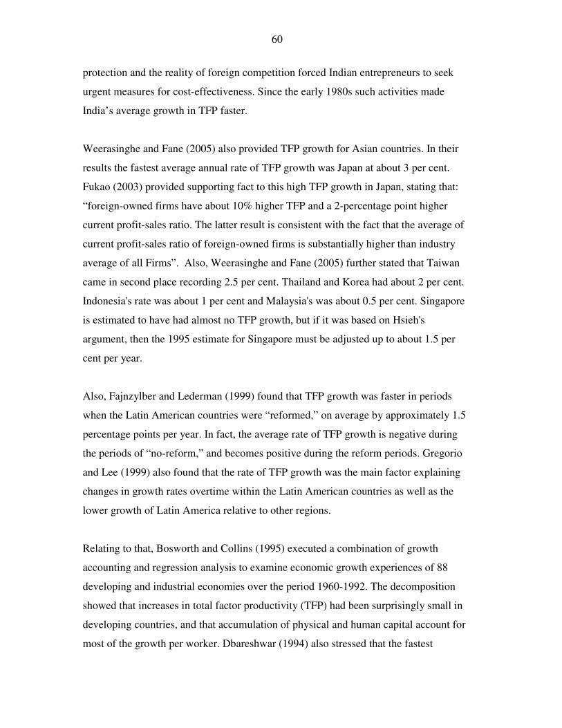
60

protection and the reality of foreign competition forced Indian entrepreneurs to seek

urgent measures for cost-effectiveness. Since the early 1980s such activities made

India’s average growth in TFP faster.

Weerasinghe and Fane (2005) also provided TFP growth for Asian countries. In their

results the fastest average annual rate of TFP growth was Japan at about 3 per cent.

Fukao (2003) provided supporting fact to this high TFP growth in Japan, stating that:

“foreign-owned firms have about 10% higher TFP and a 2-percentage point higher

current profit-sales ratio. The latter result is consistent with the fact that the average of

current profit-sales ratio of foreign-owned firms is substantially higher than industry

average of all Firms”. Also, Weerasinghe and Fane (2005) further stated that Taiwan

came in second place recording 2.5 per cent. Thailand and Korea had about 2 per cent.

Indonesia's rate was about 1 per cent and Malaysia's was about 0.5 per cent. Singapore

is estimated to have had almost no TFP growth, but if it was based on Hsieh's

argument, then the 1995 estimate for Singapore must be adjusted up to about 1.5 per

cent per year.

Also, Fajnzylber and Lederman (1999) found that TFP growth was faster in periods

when the Latin American countries were “reformed,” on average by approximately 1.5

percentage points per year. In fact, the average rate of TFP growth is negative during

the periods of “no-reform,” and becomes positive during the reform periods. Gregorio

and Lee (1999) also found that the rate of TFP growth was the main factor explaining

changes in growth rates overtime within the Latin American countries as well as the

lower growth of Latin America relative to other regions.

Relating to that, Bosworth and Collins (1995) executed a combination of growth

accounting and regression analysis to examine economic growth experiences of 88

developing and industrial economies over the period 1960-1992. The decomposition

showed that increases in total factor productivity (TFP) had been surprisingly small in

developing countries, and that accumulation of physical and human capital account for

most of the growth per worker. Dbareshwar (1994) also stressed that the fastest

61

growing developing economies have based their growth more on the rapidity with

which they have accumulated physical and human capital than on high TFP.

Furthermore, Bosworth and Collins (1995) showed that their regression results strongly

support the growing consensus that stable, orthodox macroeconomic policy, combined

with outward oriented trade policies foster economic growth. They explore the channels

through which determinants of growth operate. They found out that larger budget

deficits slow growth through reducing capital accumulation, while real exchange rate

volatility operates mainly through slowing TFP growth. Outward orientation appears to

work through both channels.

4. Conclusion

Growth accounting is a dominant device and useful in the analyses of growth rates.

Factor accumulation (capital and labour), contributes more to Kiribati’s growth than

TFP. The average growth rate of factor accumulation stood at 3% compared with the

TFP average negative growth rate of 3%. The absence of growth from TFP is a

combination of factors such as the private sector is underdeveloped; there is no

economies of scale; no manufacturing industries and no major institutional reforms that

will encourage investment and protection from international competition still in

imposition. The reported growth accounting results may also provide some policy

options to Kiribati relating to its economic growth policies.

62

6. SOLOW MODEL AND ITS EXTENSION 1. Introduction

The purpose of this chapter is to explore the use of the Solow model and its extended

versions. This is an unexplored area for PICs except for Fiji by some University of the

South Pacific economists like Rao, Singh and Saten and Rao and Rao (2006). In doing

so, we examine and analyze the significance of export ratio, remittance ratio and aid

ratio, besides the two basic conditioning variables viz., capital (K) and labour (L), for

output and its growth rate in Kiribati. In this respect, the aforesaid USP applied growth

methodology differs from many ad hoc applications where growth rate is simply

regressed on any variable or variables without incorporating the conditioning variables

into their specifications. At the least this amounts to gross misspecification and the

effects of the selected variables may be overestimated. Such ad hoc studies are too

many to cite.1 We shall later use one or two examples to illustrate the consequences of

these ad hoc specifications.

The aforesaid USP methodology of Rao et al is similar to the Mankiew, Romer and

Weil (1992), MRW hereafter, extension to the Solow model by augmenting with a shift

variable human capital (HK), into the neo classical production function. MRW found

out that the “measure of our ignorance” (the Solow residual) could be considerably

reduced without the need for changing the basic simplifying assumptions of the Solow

model. Acemoglu (2004) considers the work of MRW as an attempt to revive the

usefulness of the basic Solow growth model; see also Bernanke and Gurkaynak (2001);

��Often these authors are somewhat sensitive to criticisms on their ad hoc methodologies and uncritically

accept time series econometric results.

63

Rao and Singh and Nisha (2006) and Asteriou and Price (2004). Our attempt in this

thesis follows the USP methodology of Rao et.al i.e., make an attempt to apply the

MRW approach (to cross section data) for the time series data.

At the outset, it may be stated that although it is desirable to use a few alternative

methods of estimating cointegrating equations, only the general to specific approach

(GETS) and the Johansen Maximum Likelihood techniques yielded meaningful results

for our data. Furthermore we have used the instrumental variable approach in GETS to

minimize any endogenous variable bias. Needless to say these two techniques are

second to one. Nevertheless, given the exploratory nature of our attempt, whatever

policy implications are derived from our empirical estimates need further

investigations. Therefore, our findings should be interpreted cautiously.

The structure of this chapter is as follows. Section 2 discusses unit root results and

cointegration. Section 3 analyzes the model and empirical results are in sections 4 and

5. It concludes in section 6.

2. Unit Roots and Cointegration

The purpose of unit root tests is to test for the stationarity of a time series. Stationary

series are said to be integrated of order zero I(0). There are numerous unit root testing

procedure, each claiming that it has more power against the null of unit root in a

variable. Therefore, we shall use some popular alternative tests to test for unit roots in

our variables viz., output per worker, capital per worker, export ratio (export divided by

output), aid (ratio to output) and remittance ratio (remittance divided by employment).

In doing so, the following tests are used namely the augmented Dickey Fuller (ADF),

the ADF with generalized least squares (ADFGLS) of Pantula which is more powerful

than OLS ADF, the Phillips-Perron non-parametric test (PP), KPSS and the Elliot-

Rothenberg-Stock test (ERS).2 These tests did not yield uniform results, but it is

2 I acknowledge Professor Bill Rao in providing software for unit root test and comments.

64

generally believed that ADFGLS and ERS are more powerful and these two indicate

that all our variables are unit root variables.

Our unit root test results are as follows. The null hypothesis of unit root is rejected in

first difference in all of the variables except for dlogk under the ADF, PP and KPSS.

Also logk has unit root for other tests except under KPSS at 10 per cent critical value.

Likewise, the computed test statistics for the ERS are more than the 5 per cent critical

values, implying that all the levels of the variables are non-stationary. In essence, the

null hypothesis in all tests except in ADFGLS and ERS is that the variables are non-

stationary. The variables in their first difference under the ADFGLS and ERS are all

stationary, meaning that they are I(1). Since the ADFGLS and ERS are more powerful,

we conclude that we should apply time series methods of estimation. Otherwise the

summary statistics of the estimates will be biased and unreliable.

Table 1. Unit Root Tests Results (p-values are in the parentheses)

VARIABLES ADF ADFGLS PP KPSS ERS

ln (Y/L) -3.426 (-3.549)

-2.950 (-3.190)

-2.533 (-3.544)

0.094 (0.146)

7.007 (5.720)

ΔΔΔΔln (Y/L) -4.247 (-2.951)

-4.313 (-1.951)

-4.059 (-2.951)

0.091 (0.463)

1.502 (2.970)

ln (K/L) -2.585 (-3.548)

-2.614 (-3.190)

-1.785 (-3.544)

0.144 (0.119**)

6.481 (5.720*)

ΔΔΔΔln (K/L) -2.503 (-2.951)

-2.431 (-1.951)

-2.642 (-2.951)

0.125 (0.463)

2.939 (2.970)

ln EXRATIO -2.480 (-3.544)

-2.563 (-3.190)

-2.330 (-3.544)

0.182 (0.146)

9.295 (5.720)

ΔΔΔΔln EXRATIO -6.198 (-2.954)

-6.231 (-1.951)

-10.435 (-2.951)

0.384 (0.463)

0.659 (2.970)

ln AIDRATIO -1.749 (-3.544)

-1.127 (-3.190)

-1.754 (-3.544)

0.174 (0.146)

84.246 (5.720)

ΔΔΔΔln AIDRATIO -5.096 (-2.951)

-5.101 (-1.951)

-5.175 (-2.951)

0.548 (0.463)

1.495 (2.970)

ln RERATIO -1.310 (-3.544)

-0.842 (-3.190)

-1.332 (-3.544)

0.171 (0.146)

116.725 (5.720)

ΔΔΔΔln RERATIO -3.871 (-2.951)

-3.438 (-1.951)

-3.387 (-2.951)

0.425 (0.463)

1.793 (2.970)

Notes: (1) Figures in brackets are the critical values at the 5% level denoted by *, but in most cases the * sign is not used and figures without that sign are also at the 5% level. Figures in some brackets with a double star sign (**) show critical values at 10%

65

level. (2) In EViews the trend and intercept are included for testing unit root in level form, while as in first difference only intercept is included. (3) Also ln is the same as log and Dln is also known as Δln, which represents the first difference of a variable.

2.1. Cointegration

In the circumstance where variables are in the order of I(1) and therefore I(0) in first

differences, means that such variables with a long run equilibrium relationship cannot

drift very far apart in the long run because economic forces will act to correct any

disequilibrium (see Bierens (2006); Felmingham and Jackson (2003)). In other words,

the concept of cointegration is developed from the belief that certain economic

variables should not diverge from each other by too far a distance or diverge without

bound (see Liow (2004)). Any linear combination of I(1) variables is typically spurious.

However if there is a long-run relationship, errors have tendency to become small and

return to zero i.e. are I(0).

Nevertheless, having determined the order of integration for each variable of the time

series as per the unit root test results from the ADFGLS and the ERS techniques in

Table 1 above, we next employ all the popular techniques of cointegration to estimate a

baseline equation or to examine the existence of long run and short run dynamic

relationships based on the error correction adjustment model (ECM), to obtain

meaningful relationships between the level of output (and by implication its rate of

growth) and its determinants. The GETS, Engle-Granger, Fully Modified Ordinary

Least Squares (FMOLS) and JML VECM are used. However, only GETS and JML

VECM have given plausible results. These techniques will be used in the rest of this

chapter to examine whether or not the variables like aid ratio, export ratio and

remittance ratio have any effects besides the basic inputs of labour and capital assuming

constant returns to scale. To conserve space we shall not report results with FMOLS

and Engle-Granger methods.

66

3. The Model

In this empirical work, the basic Solow model and its extensions are used. Therefore,

some restrictions should be noted. Firstly, unlike in the cross section work with the

Solow model where the steady state growth equation is estimated, what is estimated in

time series work is the basic Cobb Douglas production function and not a growth

equation. Because of the transformations necessary to use time series methods (to

overcome unit root problem), the dependent variable is the rate of growth of output.

This does not mean that the estimated equation is the steady state growth equation and

many applied workers mistake this to be so. This is not correct. What is estimated in

time series models is the steady state production function. To derive steady state growth

equation, this production function should be combined with other equations in the

Solow growth model. Second, we also assume that there are constant returns. Third,

additional variables, such as the export ratio etc., are introduced into the model as shift

variables in the production function. We feel that it is adequate for our purpose

although these additional variables can be introduced into the production function in

other different ways.

Essentially we follow Rao and Rao (2006) and our basic production function with

constant returns and Hicks neutral technical progress is:

Yt = At Ktα Lt

1-α

= A0egt Kt

α Lt

1-α (1)

where A0 represents the initial stock of knowledge, t is time, K is capital and L is

labour.

An important assumption for illustrative purpose is that the stock of knowledge not

only changes with time but also depends on a shift variable Z. For example this Z could

be education or the ratio of exports or the ratio of aid to output. Now Z may have a

permanent and/or a temporary effect on output. To distinguish between the temporary

and permanent effects of Z, these two procedures are important. The first procedure is

67

to include Z in the cointegrating equation with capital and labour inputs. The latter two

variables may be treated as the conditioning variables. One should note that ignoring

them could cause serious misspecification and the estimates are unreliable. If there is

no cointegrating equation with Z, K and L but there is a cointegrating equation with

only K and L, then Z has no permanent effects on Y.

The second procedure is that, to test if Z has a temporary effect, its rate of change may

be included into the short run dynamic equation based on the lagged residuals of the

cointegrating equation and the error correction mechanism (ECM) adjustment process.

If Z has no temporary effect, then changes in Z and its lagged values will have

insignificant coefficients.3

This specification (intercept and trend are ignored for convenience) based on the GETS

shows how the (long and/or short run) effects of Z on Y can be captured and tested.

ΔlnY = -λ(lnYt-1 – (β1ln Kt-1 + β2lnL t-1 + β3lnZ t-1 )) + �γn ΔlnKt-n +

�γjΔlnLt-j + �γmΔlnZt-m + �γkΔlnYt-(t-(k+1) (2)

If Z has both permanent and short run effects then 3β and some mγ would be significant.

If Z has only permanent effects 3β would be significant and if Z has only short run

effects then 3β would be insignificant while some mγ would be significant.

4. Empirical Results 4.1. The Solow Model with GETS The London School of Economics-Hendry’s general to specific approach (GETS) is

widely used with its autoregressive distributed lag structure and the error correction

mechanism of adjustment. We shall estimate the GETS based specifications with the

non-linear instrumental variable method to minimize endogeneity bias. On the other

hand, the GETS method has also been criticized. This is due to the fact that there was

no cointegration test and it estimates equations with both I(0) and I(1) variables.

3 . I acknowledge Professor Bill Rao for suggesting these alternatives.

68

However, the recent work by Ericsson and MacKinnon (2003) who have developed

cointegration tests for GETS equations, which is an extension of the well known

MacKinnon tests (1991) for the Engle-Granger equations make those criticisms

untenable now.

First we estimate a baseline equation with only the two inputs viz., capital and labour.

We include an intercept and trend and retrain the constant returns constraint, but

without any Z shift variable. This yields the baseline estimate for subsequent

comparisons. However, a shift dummy is included for a break in the intercept term

because since 1990 there seems to be a break in the trends of many of our variables.4

The specification for the baseline equation is as follows.

Δlnyt = α0 + α1T - λ(lnyt-1 –(β1lnkt-1)) + �γiΔlnkt-i + �γnΔlnYt-(n+1)

+ γDUM90 (3a)

where DUM90 is one after 1990 and zero before and T is time trend. The lower case

letters are in per worker values. Thus ( / ) ( / )y Y L and k K L= = etc. The estimate of

this baseline equation for the period 1970-2005 is as follows:

Δlnyt = 4.291 - 0.030T -0.721(lnyt-1 - .337lnkt-1) + .467Dlnyt-1 -3.213Dlnkt-2 (4.4)* (-5.3)* (7.5)* (3.0)* ( 6.9)* (-4.0)*

- 0.271dum90. (3b) (-4.7)*

R bar2 =0.53; GR bar2=0.50, Sargan's CHSQ(8)=8.850[p=0.355]

SER=0.117; �2sc=4.42 (0.035); �2

ff = 3.14 (0.076); �2n = 0.38 (0.83),), �2h = 19.933(0.00).

* indicates significance at 5% level.

The above estimate indicates that this baseline equation is satisfactory (for full details

refer to Table 1A in the appendix). All the coefficients are significant at the

conventional 5% level. The R bar square and the GR bar square are close, indicating

4 Cointegration with structural breaks is both hard and often misused. As far as we are aware, such tests by Gregory and Hansen (1996) are available for only the Engle-Granger equations and not for GETS and the JML VECM models.

69

that the specification and selected instrumental variables are appropriate. This is further

confirmed by the Saragan Chi-square test, which is insignificant. The summary chi-

square tests show that there is some serial correlation at the 5% but not at the 1% level.

Because there is heteroscedasticity in the residuals, the t-ratios are White adjustment

based. The standard error of regression (SER), although high, is plausible for a small

island country where output growth rate is highly volatile. In addition, the estimate of

the adjustment coefficient lambda is highly significant with a t-ratio of 7.5, which

exceeds the Ericsson-MacKinnon critical value at the 5% level. Thus per worker output

and capital variables are cointegrated. The error correction coefficient is –0.721, which

is less than one signifies that convergence to equilibrium will be smooth. Also, the

dummy variable has a negative and significant coefficient implying that output has

declined by 0.27 per cent since 1990 due to the following factors. The government

major commercial fishing company (Te Mautari Ltd) was closed down in late 1980s

coupled with the cessation of phosphate mining for export, low world copra price

prevailed affecting the copra industry and an escalating trade deficit caused by the

increasing import of consumable items etc. Another noteworthy, although

disappointing, finding is that the rate of TFP captured by the coefficient of trend (T) is

negative implying that in Kiribati efficiency has declined with time at the rate of 3 per

cent per year. This may be due to lack of good management skills, closed down and

unproductive investments to which we referred to earlier and due to the immigration of

skilled workers elsewhere. The implied profit share of 0.337 is plausible and very close

to our stylized value of one-third in the growth accounting exercise. The actual and

predicted values of output growth are shown below in Figure 1, which seems to be

satisfactory.

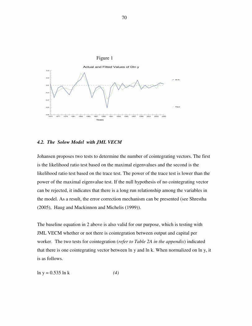
70

Figure 1

Actual and Fitted Values of Dln y

DLYL

Fitted

Years

-0.2

-0.4

-0.6

-0.8

0.0

0.2

0.4

1975 1977 1979 1981 1983 1985 1987 1989 1991 1993 1995 1997 1999 2001 2003 2005

4.2. The Solow Model with JML VECM

Johansen proposes two tests to determine the number of cointegrating vectors. The first

is the likelihood ratio test based on the maximal eigenvalues and the second is the

likelihood ratio test based on the trace test. The power of the trace test is lower than the

power of the maximal eigenvalue test. If the null hypothesis of no cointegrating vector

can be rejected, it indicates that there is a long run relationship among the variables in

the model. As a result, the error correction mechanism can be presented (see Shrestha

(2005), Haug and Mackinnon and Michelis (1999)).

The baseline equation in 2 above is also valid for our purpose, which is testing with

JML VECM whether or not there is cointegration between output and capital per

worker. The two tests for cointegration (refer to Table 2A in the appendix) indicated

that there is one cointegrating vector between ln y and ln k. When normalized on ln y, it

is as follows.

ln y = 0.535 ln k (4)

71

Equation 4 implies that the share of profit is 0.535, which is higher than 0.337 of

GETS, but this higher estimate is also plausible. The JML VECM parsimonious

dynamic adjustment equation for this version with trend is as follows (refer to Table 3A

in the appendix).

�LYL = 2.24 - 0.02T - 0.525ECMt-1 -2.39�LKL t-1 -0.23DUM90 (4.96)* (-3.48)* (-4.91)* (-2.67)* (-1.94)** (5) R bar2= 0.439; SER=0.137; �2

sc= 1.2359[.266]; �2n=1.9869[.370]

�2ff=11.4778[.001]; �2h=4.2993[.038, * and ** indicates significance at the 5% and 10%

level respectively.

The result from the above JML VECM baseline equation is satisfactory. Although the

R bar square is slightly less than the GETS equation, the actual and fitted values are

reasonably good. As in the GETS equation, the dummy variable recording a negative

coefficient of -0.253 and the coefficient of trend of negative -0.023, are higher than the

coefficients of a dummy and trend in the JML VECM in equation 5 above. Thus this

equation also implies that technical progress in Kiribati has been negative. Moreover,

the coefficient of the error correction term in the JML VECM is -0.53, which is similar

with the ECM in the GETS of -0.72, meaning that convergence to equilibrium will also

be smooth. The plot of actual and fitted values is in figure 2.

Figure 2

Actual and Fitted Values Dlny with JML VECM

DLYL

Fitted

Years

-0.2

-0.4

-0.6

-0.8

0.0

0.2

0.4

1972 1974 1976 1978 1980 1982 1984 1986 1988 1990 1992 1994 1996 1998 2000 2002 2004

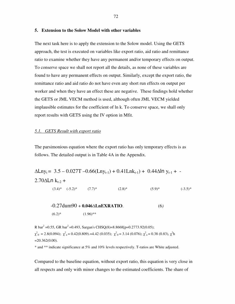
72

5. Extension to the Solow Model with other variables

The next task here is to apply the extension to the Solow model. Using the GETS

approach, the test is executed on variables like export ratio, aid ratio and remittance

ratio to examine whether they have any permanent and/or temporary effects on output.

To conserve space we shall not report all the details, as none of these variables are

found to have any permanent effects on output. Similarly, except the export ratio, the

remittance ratio and aid ratio do not have even any short run effects on output per

worker and when they have an effect these are negative. These findings hold whether

the GETS or JML VECM method is used, although often JML VECM yielded

implausible estimates for the coefficient of ln k. To conserve space, we shall only

report results with GETS using the IV option in Mfit.

5.1. GETS Result with export ratio

The parsimonious equation where the export ratio has only temporary effects is as

follows. The detailed output is in Table 4A in the Appendix.

�Lnyt = 3.5 – 0.027T –0.66(Lnyt-1) + 0.41Lnkt-1) + 0.44�ln yt-1 + -

2.70�Ln kt-2 +

(3.4)* (-5.2)* (7.7)* (2.8)* (5.9)* (-3.5)*

-0.27dum90 + 0.046�LnEXRATIO. (6)

(6.2)* (1.96)**

R bar2 =0.55, GR bar2 =0.493, Sargan's CHSQ(8)=8.8668[p=0.2773.92(0.05);

�2ff = 2.8(0.094); �2

n = 0.42(0.809).=4.42 (0.035); �2ff = 3.14 (0.076); �2

n = 0.38 (0.83), �2h

=20.362(0.00).

* and ** indicate significance at 5% and 10% levels respectively. T-ratios are White adjusted.

Compared to the baseline equation, without export ratio, this equation is very close in

all respects and only with minor changes to the estimated coefficients. The share of

73

profits increased marginally to 0.41 from 0.337. It is noteworthy that the coefficient of

�LnEXRATIO is significant at only the 10% level. This equation implies that a 10%

increase in export ratio will increase growth in output temporarily by about half a

percent. Such low increase in output may be due to the fact that any increase in exports

fail to have any significant backward and forward linkage effects in Kiribati.

When the JML VECM approach is used, the null hypothesis of no cointegration vector

is rejected at the 5 and 10 per cent levels and the null of one cointegrating vector is not

rejected. However, the cointegrating vector showed that the coefficient of export ratio

is negative and the share of profit is 5. These are implausible values and the output is in

table 5A in the Appendix. Therefore, there is no meaningful long run relationship

between export ratio and output.

5.2. GETS Result with aid

To put into perspective, it is worth considering having a proper GETS specification

with aid, with linear and then a non-linear specification of aid (refer to table 6A in the

appendix). Results with only a linear aid term are significant and the results are as

follows.

ΔlnY =2.93 – 0.04T – 0.73(lnYt-1 + 0.65lnKt-1 –0.07lnRAIDlt-1)

(1.28) (-4.31)* (5.56)* (1.96) (-2.46)*

+ 0.44ΔlnYt-1 -3.69ΔlnKt-2 -0.338dum90 -0.31ΔlnRAIDl (7)

(3.36)* (-4.49)* (-3.53)* (-1.81)

R bar2 = .23981; GR-bar2 = .45515;SER = .14983; �2sc = 4.6579[.031]; X

2ff = 3.1585[.076]; �2

n =.40260[.818]; �2

h = 4.2257[.040].

It can be seen that all the coefficients are significant, but the effects of aid, in both long

and short runs, is negative. It is pointless to think about how large are these negative

effects and the results support Professor Hughes (2003) concerns that aid has been

74

unproductive in many island countries. Estimation on the effects of aid was also

executed with JML VECM but none of the options yielded any sensible results.

5.3. GETS Result with remittances

GETS specifications with linear and non-linear remittance terms are estimated but the

linear specification gave better results although the coefficient of capital is

insignificant. Therefore, we re-estimate by constraining that the coefficient of capital is

0.337, which is the estimate in the baseline equation (refer to table 7A and 8A in the

appendix). The following is the result.

�LYL = 5.39 - 0.033T -0.83(LYLt-1 -0.337LKLt-1 -0.097LRREMLt-1) + 0.41�LYLt-1

(5.97)* (-5.59)* (7.3)* (constrained) (4.6)* (-5.9)*

-0.38dum90 -0.335�LRREML (8)

(-5.99)* (-1.4)

R bar2=.48010;GR-Bar2 =.53615; SER =.12391; �2sc=3.0260[.082]; X

2ff=4.8827[.027];

�2n=.50889[.775]; �2

h = 12.2192[.000]. As can be noted the long run effect of remittance is negative and significant. Although

its short run effect is negative it is insignificant. Therefore, we removed the short term

effect and estimated the equation. However, the coefficient of remittance has become

insignificant. We also tried to estimate an equation in which remittance has only short

run effect, but this equation was unsatisfactory and although the coefficients of changes

in remittances were negative they were all insignificant. Therefore, we may say that

remittances like aid, remittances have only negative permanent effects.

75

5.4. Ad hoc specifications

In order to get an idea of the nature of ad hoc specifications, we used JML VECM to

test the effects of aid in an ad hoc manner.5 The assumed ad hoc specifications are: lny

= a+b ln aid and lny = a+b ln aid +c ln aid2 . While there was no cointegrating vector in

the linear specification, the trace and eigen value tests showed that there is one

cointegrating vector in the non-linear specification (refer to table 9A in the appendix).

Normalized on output, this cointegrating equation is:

ln y =21.918 ln aid -1.583 (ln aid)2 (9)

This implies that the maximum effect of aid per worker is reached when log of aid per

worker is about 7. The plot of this effect is given in figure 3 below where x = log of aid

per worker and on the vertical axis its effect on output worker is shown.

Although this result looks impressive it should be noted that the implied elasticity of

output per worker with respect to aid per worker is implausibly high. In 2005 the value

of log aid per worker is 5.5765 and the elasticity at this value is 4.27, implying that a

10% increase in aid will cause about 43% increase in per worker output! Similar results

were also found with JML VECM, by Jayaraman and Choong (2006), with ad hoc

specifications, that a 1% increase in per capita aid for Fiji will increase per capita

output by 65%! Such results with ad hoc specifications are not only unreliable but

show how many applied economists are mesmerized with techniques and pay little

attention to interpretation and evaluation of their findings. Rao (2006) consider some of

these pitfalls in applied econometric work with time series econometrics.

5 There are several other ad hoc specifications in which growth of output is simply regressed on aid etc

and the equation is estimated with OLS. We shall not examine all such ad hoc specifications.

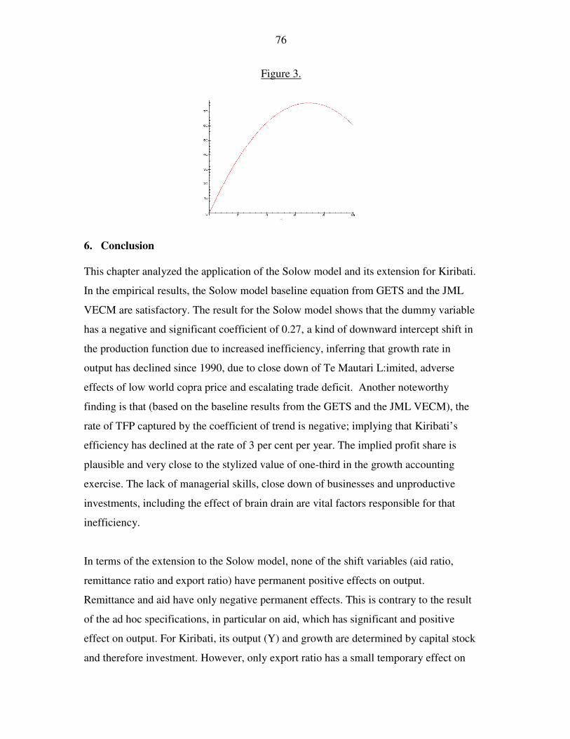
76

Figure 3.

�

6. Conclusion This chapter analyzed the application of the Solow model and its extension for Kiribati.

In the empirical results, the Solow model baseline equation from GETS and the JML

VECM are satisfactory. The result for the Solow model shows that the dummy variable

has a negative and significant coefficient of 0.27, a kind of downward intercept shift in

the production function due to increased inefficiency, inferring that growth rate in

output has declined since 1990, due to close down of Te Mautari L:imited, adverse

effects of low world copra price and escalating trade deficit. Another noteworthy

finding is that (based on the baseline results from the GETS and the JML VECM), the

rate of TFP captured by the coefficient of trend is negative; implying that Kiribati’s

efficiency has declined at the rate of 3 per cent per year. The implied profit share is

plausible and very close to the stylized value of one-third in the growth accounting

exercise. The lack of managerial skills, close down of businesses and unproductive

investments, including the effect of brain drain are vital factors responsible for that

inefficiency.

In terms of the extension to the Solow model, none of the shift variables (aid ratio,

remittance ratio and export ratio) have permanent positive effects on output.

Remittance and aid have only negative permanent effects. This is contrary to the result

of the ad hoc specifications, in particular on aid, which has significant and positive

effect on output. For Kiribati, its output (Y) and growth are determined by capital stock

and therefore investment. However, only export ratio has a small temporary effect on

77

output and the result from the GETS implies that a 10% increase in export ratio will

increase per capita output to about 0.5 % annually. This empirical result confirms the

answer to the research question on what the determinants of the growth rates in Kiribati

are.

Furthermore, there are notable reasons why aid and remittances have no positive

permanent and/or short run effects on Kiribati’s output. Both are channeled to

consumption. Aid has been channeled to unproductive investment as earlier reported

based on the finding of the high capital-output ratio and the current criteria of providing

aid by aid-donors, which also supports Hughes (2003) assertion. Moreover, Lloyd and

Morrissey and Osei (2001) reported their empirical finding in Ghana saying that the

coefficient of aid on growth is insignificant. Any impact of aid on short-run growth was

negligible. Also, the level of income in Kiribati is very low and the remittances

normally channel to the families of seafarers for their living, which are utilized for their

consumption, implying that there is likely no saving by the majority of seafarers for

business purposes. Currently, there is no provident fund for these seafarers and it is

significant that arrangement be made on it for their future activities.

In order to increase the contribution of export to output, will require more and higher

export earnings. The increase in domestic productive investment such as value added

products from the available natural resources is an area to be considered. For example,

it can be in processing or semi-processing fish and other available domestic resources

for overseas markets.

In terms of improving the contribution of aid to productive investment, it can be as

investment in joint projects, which does not only increase K, but also because of more

efficient management skills & technology acquired, may improve TFP. This implies the

need to have foreign direct investment in Kiribati, and since we have bilateral

diplomatic ties with most of the developed and fast growing economies, such as

Australia, New Zealand, Taiwan and Japan etc, these countries may consider

78

encouraging a few firms in their countries to invest in Kiribati under bilateral economic

cooperation aimed for economic development. This also applies to multilateral aid.

More over such aid donors may allocate some of their aid in financing machineries,

technical expertise etc to entrepreneurs and entrepreneurs’ training for establishing their

small-scale manufacturing industries, which can be expanded if successful by owner’s

expenditure. Likewise, aid donors may render assistance to fund public productive

investment. It is also significant that both aid donors and the host government may even

provide financial incentives to foreign firms and local entrepreneurs.

The operational mechanism for this framework of cooperation will be under the joint

responsibility of aid donors and government. Therefore, part or much of the aid can be

in this form, which renders the foundation for cooperation called “Cooperation

between Aid donors and Government for Economic Development through Productive

Investment and Increasing Participation of the Private Sector”. Currently, the Pacific

Islands Forum leaders persuade Australia to allow recruiting seasonal workers to be

employed in her economy. Although there are benefits from this proposed scheme, it

does not solve the root of the economic problem of low growth rate in the Island

economies, but create more dependency on external economies, which may be unstable

in the long term. What the PIF leaders should consider is to convince aid donors to

develop the economies of the Island countries, through allocating their aid in productive

investment, in order to be able to provide employment and income for their population

in the long term.

Investing more in productive investment domestically based on the right economic

policies, will mean that the economy will be more productive, and can have sustained

economic growth when such productive investment have management and technical

expertise as well as embodied or embraced technological advance in their industries in

the long term.

79

7. CONCLUSION 1. Introduction

In this thesis we have examined what the main factors that determine the growth rate in

Kiribati are. We have used the Solow growth model and its extensions as are our

framework for the empirical study. However, given various constraints, especially data

limitations, this thesis has concentrated on the two conditioning variables viz., labour

and capital and examined the long and short run effects of three additional variable viz.,

exports, aid and remittances. Our main findings, subject to several caveats, are that (a)

technical progress in Kiribati has been negative, (b) capital per worker adequately

explains output per worker (c) neither aid nor remittances have significant long or short

run effects on the level of output and (d) exports seem to have only a small and

significant short run effects on output. In this process we have shown that the simple

Solow framework can be usefully extended to explain the determinants of output in a

small island country like Fiji.

2. Summary of Quantitative Results

How can we assess the performance of Kiribati’s output? The findings from our growth

accounting exercise, which can show the growth from factor accumulation and total

factor productivity is important on that area. Factor accumulation contributes more to

Kiribati’s output growth due to its higher average growth rate of 3% per annum than the

TFP, which recorded an average growth rate of negative –3% per annum. This makes

the net growth rate of Kiribati almost insignificant.

The major reason for this disparity includes: The absence of growth from TFP, implies

the underdevelopment of the production sector, mainly the private sector, the absence

80

of economies of scale, no major institutional reforms and protection from international

competition remain in imposition.

What are the determinants of the growth rates in Kiribati? The result from the growth

accounting is also significant. However, the empirical findings after using the applied

econometric and conforming to the Solow model and its extensions are satisfactory.

The result for the Solow model shows that the 1990 dummy variable has a negative and

significant coefficient of 0.27, a kind of downward intercept shift in the production

function due to the increased inefficiency, inferring that growth rate in output has

declined since 1990. Some relevant reasons are: Government public enterprises such as

Te Mautari Ltd catered for commercial production had been closed down in late 1980s.

Also, there is adverse effect of low world copra price on copra production, thus export

earnings plummeted. Further more, given the narrow export base, the trade deficit

escalated, meaning that Kiribati depends heavily on overseas countries for aid, foods

and goods etc. Another noteworthy finding is that (based on the baseline results from

the GETS and the JML VECM), the rate of TFP captured by the coefficient of trend is

negative; implying that Kiribati’s efficiency has declined at the rate of 3 per cent per

year, which is the same with the growth accounting results. The implied profit share is

plausible and also very close to the stylized value of one-third in the growth accounting

exercise. The lack of managerial skills, close down of businesses and unproductive

investments, including the effect of brain drain are vital factors responsible for that

inefficiency.

The results from the extension to the Solow model show that none of the shift variables

(aid ratio, remittance ratio and export ratio) have permanent positive effects on output.

Remittance and aid have only negative effects. This is contrary to the result based on

ad hoc specifications, where some works found that aid has significant and positive

effect on output. For Kiribati, its output (Y) is determined by capital stock and therefore

investment. However, the export ratio has a small temporary effect on output and the

result from the GETS implies that a 10% increase in export ratio will increase per

81

capita output by about 0.5 % annually. Based on this empirical result, we can provide

answer to the determinants of the growth rates in Kiribati.

The justification for aid and remittances for being not contributing much to growth in

Kiribati include the followings. Aid has been channeled to unproductive investment and

consumption. This is justified by the finding on the high capital-output ratio and the

current criteria of providing aid by aid-donors, which also supports Hughes (2003)

assertion. Unemployment and the very low income in Kiribati make the remittances

fully utilized on consumption by the seafarers’ families.

3. Some Data Limitations

Applied econometric work requires time series macroeconomic data depending on the

nature of the study. In Kiribati the formulation and compilation of time series data on

macroeconomic variables are incomplete and not up to date. Only the data for the

export of copra, transformed into the export ratio, in the form of export earnings and

annual production are available. The major time series data source for Kiribati’s GDP

and its components are obtained from the United Nations Statistic Department website,

while employment, remittance and foreign aid figures are available locally, having

more than half of the time series data from 1970 to 2005 requirement. The rest are

estimated in compliance with estimate from the Taxation office of the Kiribati

government, population census report of the Statistic office and figures from external

sources. Therefore, given this circumstance, the result of the empirical study should be

interpreted cautiously; unless we have a more reliable source for time series data.

4. Additional Observations

The theories of economic growth are significant in the understanding of disparity

between economic growth rates and development between different countries. The

Solow model and its extensions are useful for that purpose, embracing as well the

MIRAB model, which specifically reflects the stylized facts of the Island Economies in

82

the South Pacific, although it defaulted to stress the correct source for the remittance in

Kiribati, which is mainly from the seafarers.

Kiribati’s foreign exchange earnings from the access fee, foreign aid, remittances and

the draw down from the RERF and trade openness are significant, given the

underdevelopment of the private sector to provide employment, income and

government’s revenue, for the development and sustainability of Kiribati’s economy.

The revenue equalization reserve fund (RERF), the access fee and export earnings have

more direct positive effects on government financing requirement, while the foreign aid

and remittances are channeled to consumption.

There are issues concerning the sustainability of such significant foreign exchange

earnings. Firstly, they are vulnerable to short run fluctuations from external economies,

instability in the financial capital markets, weather and diplomatic ties. For instance, the

RERF is susceptible to instability in the financial capital markets. The revenue from the

access fee depends heavily on the weather pattern, which affects the location of tuna

species in the ocean. More over, the remittance and foreign aid can be unstable if a

diplomatic relationship is unfavourable with the country relying on for labour mobility,

remittance and aid. Trade openness and the export of copra etc, relies on overseas

demand, foreign income, weather, world price and stability in the economies where it

exports its copra to.

Domestically, the question is what are the other sources of government’s revenue apart

from foreign exchange earnings? Since independence, however, some meager major

reliable sources of revenue for government’s recurrent budget are on personal tax,

company tax, and other fees and taxes, dividend shares etc. The income from personal

tax is much higher than the revenue from the company tax, implying the

underdevelopment of the private sector.

Based on such revenues determine how much the government can budget for its

expenditure. Since independence in 1979 after the cessation of phosphate mining,

83

government revenue from phosphate tax plummeted greatly. The first government

under the leadership of the National Progress Party encountered that economic

problem. Fortunately, its budget of $33 million was adequate indeed given its low

population, few employees in the public service and lower salary. As the population

increases as well as the increase in the size of the public service, require extra outlay,

and other major expenditure items promised during the campaigns, such as the increase

in the price of copra and elderly pension, put pressure on government financial

resource. These developments experienced during the government of the Maneaban Te

Mauri Party from 1994 to 2002, resulting in its recurrent budget reaching $98 million in

2002, and the same level of expenditure experienced during the government of the

Boutokan TE Koaua Party from 2003 to 2006. The increase in recurrent budget would

have adverse effects to the real value of the RERF.

On the issue of the gross domestic product and its growth rates, they were fell after the

cessation of phosphate mining, but recovered since late in the 1980s at lower level of

growth. Government expenditure provides much to GDP and its growth. In addition,

the gross national per capita income for Kiribati based on the UNSD data remains

stabilized at US$1,500.00, which falls under the category of the Least Developed

Countries. Kiribati’s GNI is lower due to limited revenue from productive sectors

abroad such as from the RERF, the access fee, the aid and the remittance. Given the

increase in the population, it has eaten up the GNI per capita. Stabilizing population has

been one area of government’s policy.

The effects of the current wave for the implementation of trade-liberalization on

Kiribati remain under consideration. The positive effects of this free trade may be

having a cheaper price for imported goods etc. Unfortunately, there is trade off. Island

economies such as Kiribati will lose out from their import duty revenue stood

approximately Australian dollar 10 million annually. How to compensate this source of

revenue? VAT and other forms of taxes may be considered. There may be price

increased on imported goods etc through the imposition of the VAT. Free trade will

maintain the productive powers of the developed countries and to keep their

84

employment and income, given the availability of their markets for their products in

other economies. For Small economies, their industries, income and employment may

be affected if they are flooded with cheaper imported goods.

5. Recommendations Based on the findings, it is worth considering suggestions on foreign exchange

earnings. These major foreign exchange earnings for Kiribati are vital for output and

should be managed prudently such as on the RERF and the access fee; render

incentives and negotiations where necessary especially on labour mobility and

employing agencies abroad and based in the country as well, and a thorough diplomatic

negotiation is required on aid for their long-term sustainability and economic benefits

to Kiribati.

In addition, aid should be provided to productive investment. Aid donors should

consider encouraging their firms to invest in Kiribati in order to develop Kiribati’s

economy. This also applies to multilateral aid. Aid donors and government should also

provide incentives to such firms. Also, the provision of machineries for small scale

manufacturing of entrepreneurs is significant. This render the basis for cooperation

called “Aid donors and government cooperation for economic development through

productive investment and increasing the participation of the private sector.” The

mechanism for this cooperation framework will be under the sole responsibility of an

aid donor and the host government.

The high level of government expenditure is not sustainable in the long term, given its

limited financial resource and only the RERF that has been the backbone of the

government for a long time. The high draw down of the RERF per annum will affect

the real value of the fund and is unsustainable. Therefore, prudent government financial

management is required.

85

Based on the empirical findings, the following recommendations are significant. In the

Solow model, Kiribati’s output and its growth rates are determined by capital stock and

therefore investment. Therefore, it is imperative to increase investment in productive

industries. Further more, given the fact that only export ratio has temporary positive

effects on output, efforts should be focus on increasing its contribution on output. This

will require more and higher export earnings. Expanding the export base to include

manufacturing of value added products from the available natural resource or semi

finished products for domestic manufacturing imported from overseas are crucial.

By investing more in productive investment, provided there is a right economic policy,

will make such economy productive, and can have sustained economic growth in the

long term when such industries have management and technical expertise, as well as

embodied technological advance. This will also improve the contribution of total factor

productivity to growth.

………

86

References Aaheim,A and Sygna, L. 2001. “Tuna Fish Catch in Pacific to Be Affected by Climate Change with vast potential economic consequences.” Norwegian Center for International Climate and Environmental Research (CICERO report 2000) on the tuna fishing industry in the Fiji Islands and Kiribati, Asia Pulse, Cebu.

Acemoglu, D., (ed.) (2004) Recent Developments in Growth Theory, Edward Elgar Publishing. Alice, W,E,D and Nakamura, O. 2002. “The measurement of aggregate total factor productivity growth”, Science handbook of econometrics, Vol 6. APO.2004. Total Factor Productivity Growth: Survey Report. Published by the Asian Productivity Organization. 1-2-10 Hirakawacho, Chiyoda-ku, Tokyo 102-0093. Area - land ranking of countries @ http://www.photius.com/rankings/geography/total_land_area_2004_1.html

Asian Development Bank (ADB).2002. Kiribati Discussion Paper on Assessment of Hardship and Poverty (Nov-02);

___________. 2002. Kiribati: Monetization in an Atoll Society – Managing Economic and Social Change,Manila ___________. 2004. Technical Assistance to the Republic of Kiribati for preparing outer island growth centers project. TAR: KIR 38138, December. Asian Development Bank outlook 2004. - http://www.adb.org/documents/books/ado/2004/prelims.asp

Asia Pacific Viewpoint. 1999. Norfolk Island. Volume 40, Number 3, December, pp. 235-249(15); Blackwell Publishing.

Asteriou, D. and Price, S., (2004) “ Financial development and economic growth: Time series evidence for the case of U.K.,” Discussion Paper 80, Department of Economics, City University, London. Banarjee, A. , Dolado, J. J., Galbraith, J. W. and Hendry, D.F., (1993). Cointegration, Error-Correction and the Econometric Analysis of Non-stationary Data, Oxford: Oxford University Press.

87

Barreto,H and Howland,F,M.2005. Introductory econometric. Cambridge University press, London - http://www.wabash.edu/econometrics/EconometricsBook/chap18.htm

�

Barro, R.J., (1991). Economic growth in a cross section of countries, Quarterly Journal of Economics, pp.407-433. ———— (1999). Determinants of Economic Growth, Cambridge, MA: The MIT Press. Beginners guide to growth accounting - http://www.amherst.edu/~econ53/growacct.pdf� Bernanke, B,S and Gurkaynak, R, S. 2001. Is growth exogenous? Taking Mankiew, Romer and Weil seriously. National science foundation. Bertram, G and Watters, R.F. 1985. “The MIRAB Economy and South Pacific Microstates”, Pacific Viewpoint 26 (3): 497-520. Bertram, G. 2004. “The Mirab Model in The 21st Century.ISLANDS of the WORLD VIII International Conference,” Changing Islands – Changing Worlds, 1-7 November, Quemoy. Bertram, G. 2006. “The MIRAB model in the twenty-first century”. Asia Pacific Viewpoint, Vol. 47, No. 1, April 2006 ISSN 1360-7456, pp1–13 Bierens, H. J. (2006), "Econometric Analysis of Linearized Singular Dynamic Stochastic General Equilibrium Models", forthcoming in the Journal of Econometrics.

Boland, S and Dollery, B. 2005. The economic significant of migration and remittances in Tuvalu; Working paper Series in Economics, UNE.

Borovnik, M.2006. “Working overseas: Seafarers’ remittances and their distribution in Kiribati”. Asia Pacific Viewpoint, Vol. 47, No. 1, April ISSN 1360-7456, pp151–161. Development Studies, School of People, Environment and Planning, Massey University, Palmerston North. Bosworth, B. and Collins, S. M., (2003). The empirics of growth: An update, Brookings Institution, September 22, 2003. Caselli F. and D. Wilson. 2002. Importing Technology, manuscript, Harvard University. Caselli, F., (2004). “Accounting for cross-country income differences” Working Paper No. 10828, National Bureau of Economic Research, Cambridge, MA., forthcoming, Handbook of Economic Growth.

88

CBO. 2002. The role of computer technology in the growth of productivity. Chand, S. and Sen, K., (2002). Trade liberalization and productivity growth: Evidence from Indian manufacturing, Review of Development Economics, pp.120-132. Chumacero, R,A and Fuentes,J,R. 2003. On the determinants of Chilean Economic Growth. Department of Economics of the University of Chile and the Research Department of the Reserve Bank of Chile. CIA- the world factbook-Kiribati-http://www.cia.gov/cia/publications/factbook/geos/kr.html Dube, S., (2004). An application of ARDL model to the determinants of economic growth in Botswana, Department of Economics, California State University, Sacramento. Duncan, R. 2004. “Managing volatile fishing license revenue in the pacific”. Pacific Economic Bulletin vol. 19 No.3 © Asia Pacific Press. Denison, E. F. (1962), Sources of Economic Growth in the United States and the Alternative Before Us (Committee for Economic Development, New York). Denison, E. F. (1967), Why Growth Rates Differ: Post-War Experience in Nine Western Countries. (Brookings Institution, Washington, DC). Denison, E. F. (1979), Accounting for Slower Economic Growth. (Brookings Institution, Washington, DC). Durlauf,S,N and Kourtellos, A and Tani, C,M.2005. Empirics of Growth and Development. Eaton, J. and S. Kortum, 2001. “Trade in Capital Goods”, European Economic Review, 45, 1195-1235. Engle, R.F. and Granger, C.WJ. 1987. “Co-Integration and Error Correction: Representation, Estimation, and Testing,” Econometrica, 55, 2, 251-76. Ericsson, N., and MacKinnon, J. (2002) “Distributions of Error Correction Tests for Cointegration,” Econometrics Journal, 5: 285-318. Fajnzylber, P and Lederman,D. 1999. Economic Reforms and Total Factor Productivity Growth in Latin America and the Caribbean, 1950-95: An Empirical Note. Felmingham,B and Jackson, N.2003.Population change and Australian living standard, Discussion paper 2003-06, School of economics.

89

Fukao, K. 2003. “Do foreign firms bring greater total factor productivity to Japan?”. Paper prepared for the conference Rapid economic growth and technology transfers, October 17-18. RIETI discussion paper serie 04-E-014. Gerhard M, G., and Verbiest,P, and Wolf, P.P.1998. Perpetual Inventory Method Service lives Discard patterns and Depreciation methods, Statistics Netherlands, Department of National Accounts Granger, C, W,J. 2003. Time Series Analysis, Cointegration, and Applications (The Nobel Lecture). Department of Economics, University of California, San Diego La Jolla. Gregory, Allan and Bruce Hansen (1996). “Residual-Based Tests for Cointegration in Models with Regime Shifts.” Journal of Econometrics 70, 99{126. Gregory, A.W., Nason J.M. and D. Watt (1994). “Testing for Structural Breaks in Cointegrated Relationships." Journal of Econometrics 71, 321{341. Gregorio, J. D and Lee J,W.1999. Economic Growth in Latin America: Sources and Prospects. Universidad de Chile and Havard University. Gregory, A,W & Hansen,B,E. 1996. “Tests for Cointegration in Models with Regime and Trend Shifts,” Oxford Bulletin of Economics and Statistics, Department of Economics, University of Oxford, vol. 58(3), pages 555-60, August. Good, L. 2003. “Aid disbursements from principal donors to Pacific ACPs and OCTs, 1999-2001: An Analysis.” Pacific Issues, Paper N° 5. Unit Dev/CA, The Pacific. Grossman, G. and Helpman, E. (1991), Innnovation and Growth in the Global Economy, MIT Press. Growth accounting - http://www.econ.ucla.edu/doepke/teaching/c32/sec1.pdf Haug, A. and Mackinnon, J,G. and Michelis, L. 1999. European Monetary Union: A cointegration analysis. University of Canterbury and York University. Hendry, D.F. and Doornik, J. A .1994. “Modeling linear dynamic econometric systems,” Scottish Journal of Political Economy,” pp.1- 33. —- and Krolzig, H.M. (2000). The econometrics of general to simple modelling, Mimeo, Economics Department, Oxford University.

90

Hughes, H. 2003. “AID HAS FAILED IN THE PACIFIC”. The Centre for Independent Studies Issue Analysis 33. IMF.2006.Global Financial Stability Report. Market Developments and Issues, September. International Monetary Fund. Jayaramann, T.K and Choong,C.2006.Aid and Economic growth in the Pacific islands: An empirical study of aid effectiveness in Fiji. University of the South Pacific working papers No.2006/15.Suva.

Jones, C, I and Scrimgeour, D.2005. The Steady-State Growth Theorem: Understanding Uzawa (1961), Department of Economics, U.C. Berkeley and NBER. Jones, C, I.2000. A note on the closed-form solution of the Solow model. Standardford University. Kiribati- http://www.ausaid.gov.au/country Klenow and Rodriguez-Clare, A. 1998. “The Neoclassical revival in growth economics: Has it gone too far?”, NBER Macroeconomic Annual, pp.73-103. Cambridge: MIT Press.

Knox, A,B. 1971. “The rise of colonial Federation as an object of British policy, 1850-1870”, Journal of British studies, vol.II, pp.92-112.

Kohn, D, L. 2005. Crisis Management: The Known, the Unknown, and the Unknowable. Remarks by governor at the Wharton/Sloan/Mercer Oliver Wyman Institute Conference, "Financial Risk Management in Practice," Philadelphia, Pennsylvania. Krugman.P.1994.The myth of Asia’s Miracle: Foreign Affairs, 73:62-78. Kundu,K,K.2005. Productivity – the key to India’s growth: http://www.atimes.com/atimes/South_Asia/ Laufa, T, M. 2005. Aid Effectiveness in Pacific Region Under Globalization – Understanding Its Dynamics. A paper presented at the Pacific Conference on Growth and Development: Building Better Pacific Economies held at the University of Papua New Guinea from 12-14, October 2005. Limam, Y,R and Miller, S, M. 2004. “Explaining Economic Growth: Factor Accumulation, Total Factor Productivity Growth, and Production Efficiency Improvement”, Department of Economics Working Paper Series 2004-20, University of Nevada, Las Vegas, and University of Connecticut. Forthcoming in Quarterly Review of Economics and Finance.

91

Liow,K,H. 2004. Dynamic relationship between stock and property markets. National University of Singapore. CRES: 2004 -002. List of countries by GDP (PPP) per capita - http://en.wikipedia.org/wiki/List_of_countries_by_GDP_(PPP)_per_capita

�

Lloyd,T and Morrissey,O and Osei, R. 2001. Aid, Export and Growth in Ghana. CREDIT research paper No.01/01. University of Nottingham.

Macdonald,B. 2001. Cinderellas of the empire: Towards a history of Kiribati and Tuvalu. Institute of pacific studies, university of the south pacific, suva.

Mackinnon,J.J.1991. Critical values for cointegration test, in readings in cointegration (ED) R.F Engle and C.W.Granger, Oxford university press, Oxford, pp.267-276.

Mackinnon, T.G.,Haug,A.A. and Michelis, L. 1999. “Numerical distribution functins of likelihood ratio test for cointegration”, journal of Applied econometrics 14:563-577. Mankiw, N.G. Romer, D. and Weil, D.1992. “A contribution to the empirics of economic growth”. Quarterly Journal of Economics, pp.407-437. Måns Söderbom and Francis Teal .2003.Openness and Human Capital as Sources of Productivity Growth: An Empirical Investigation, CSAE WPS/2003-06 Centre for the Study of African Economies, Department of Economics, University of Oxford Mamanja, D and Morrissey, O. 2006. Fiscal Policy and Economic Growth in Kenya. Working paper No.05/06. Centre for Research in Economic Development and International Trade. University of Nottingham. Meinen, G and Verbiest, P and Wolf, P,P. 1998. Perpetual Inventory Method Service lives Discard patterns and Depreciation methods. Statistics Netherlands Department of National Accounts, JM Voorburg McFetridge.1991. Foreign Investment, Technology and Economic Growth. Investment Canada Research Series, Vol.1. University of Calgary press. McGall, G.1997. “A debate and discourse from below”. Invited paper at the Cultural heritage in islands and small states Conference, Valletta, Malta, 8-10 May. Ministry of Finance and Economic Development.2000.Ana kainibaire Kiribati:National development strategy 2000-2003, Uataboa te rikirake ao te rau. Government of Kiribati printing. Bairiki. _______ .1988. Kiribati sixth development plan 1987-1991 te kan riki n toronibwai. Government of Kiribati printing. Bairiki.

92

_________.2003. National development strategies 2004-2007; Enhancing growth and ensure it equitable distribution. Government of Kiribati. Bairiki. _________.1997. Medium term strategy: An action programme for the national development strategy through to the year 2000. Bairiki. __________.2004. Government of Kiribati 2005 Budget: As presented to the Maneaba ni Maungatabu. Bairiki. __________. 2003. Government of Kiribati 2004 Budget: As presented to the Maneaba ni Maungatabu, Bairiki. __________ .2002. Government of Kiribati 2003 Budget: As presented to the Maneaba ni Maungatabu, Bairiki. __________.2001. Government of Kiribati 2002 Budget: As presented to the Maneaba ni maungatabu, Bairiki. ___________.2000. Government of Kiribati 2001 Budget: As presented to the Maneaba ni maungatabu, Bairiki. __________ .2002. Government of Kiribati supplementary appropriation (No.1) May 2002. As presented to the Maneaba ni Maungatabu. Bairiki. __________.2003.Government of Kiribati supplementary appropriation (No.1) March-April 2003: As presented to the Maneaba ni Maungatabu.Bairiki. __________ .2004.Government of Kiribati supplementary appropriation (No.2) 2004:As presented to the Maneaba ni Maungatabu.Bairiki. __________ .2004.Government of Kiribati supplementary appropriation (No.4) June 2004:As presented to the Maneaba ni Maungatabu. Bairiki. __________.2001. Government of Kiribati supplementary appropriation (No.2) Nov-Dec 2001.Bairiki. __________ .2005. Government of Kiribati supplementary appropriation (No.2) June 2005.Bairiki.

93

__________ .2000. Government of Kiribati supplementary appropriation (No.1) May-June 2000:As presented by the Maneaba ni Maungatabu, May-June 2000, Bairiki. __________.2000.Government of Kiribati supplementary appropriation (No.2) November-December 2000:As presented to the Maneaba ni MAungatabu. Bairiki. __________ .2002.Government of Kiribati supplementary appropriation (No.2) September-October 2002:As presented to the Maneaba ni MAungatabu. Bairiki. Musso, A and Westermann, T. 2005. Assessing potential output growth in the Euro area: A growth accounting perspective. Occassional paper series No.22. European Central Bank. Nehru, V and Dbareshwar, A.1994. New Estimates of Total Factor Productivity Growth for Developing and Industrial Countries The World Bank international economic department June 1994 - POLICY RESEARCH WORKING PAPER 1313 NZIER - Definition of GDP, Gross Domestic Product - New Zealand Institute of Economic Research © 2006 - ttp://www.nzier.org.nz/SITE_Default/SITE_economics_explained/GDP.asp� OECD. 2000. The Development Assistance Committee, Development Cooperation Reports, 1971-2000. Paris. Patterson, K. (2000) An Introduction to Applied Econometrics: A Time Series Approach, Baisngstoke: Palgrave. Pedroni, P. 1999. “Critical Values for Cointegration Tests in heterogeneous panels with multiple regressors”. Oxford Bulletin of Economics and Statistics, Special Issue (1999) 0305-9049.

Perez-Corral, Q,V.2001. ‘Private sector as the engine for growth : ADB’s private sector development strategy.’ Forum briefer 01-13, NGO Forum on ADB.

Pinheiro, A, C and Gill, I, S and Serven, L and Thomas, M, R.2001. Brazilian economic growth, 1900-2000 lessons and policy implications.unpublished. Rao, B. B., (2006) ‘Estimating short and long run relationships: A guide to applied economists’, forthcoming, Applied Economics. Rao, B. B and Rao, M. (2006) “Exports and Determinants of Growth Rate: Some Evidence with Time Series Data from Fiji,”, forthcoming, Applied Economics.

94

Rao, B. B., Singh, R and Fozia, N. (2006) An extension to the neoclassical growth model to estimate growth and level effects, Working Paper No. wp2006/4, School of Economics, the University of the South Pacific Research Methods - http://bubl.ac.uk/LINK/r/researchmethods.htm Sato, R. (1999a). Theory of Technical Change and Economic Invariance, Cheltenham, UK: Edward Elgar Publishing Inc., reprint, with amendments of 1981 edition.

______ (1999b), “Production, Stability and Dynamic Symmetry”: The Selected Essays of Ryuzo Sato in Economists of the Twentieth Century Series, Cheltenham, UK: Edward Elgar Publishing, Inc.

Secretariat of the Pacific Community (SPC).Pacific Islands Regional Millennium Development Goals Report 2004, Statistical Annex, available online at ( http://www.spc.int/mdgs );

Shrestha, M,B.2005. ARDL Modelling Approach to Cointegration test. University of Wollongong, New South Wales. http://www.nzae.org.nz/conferences/2005� Solow, R. 1956. A Contribution to the Theory of Economic Growth. Quarterly Journal of Economics 70 (February): 65-94. Statistic Office. 2002. Kiribati Statistical Yearbook 2002. Government of Kiribati printing. Bairiki. ___________.2001.Government finance statistic (GFS) 1985-2000. Government of Kiribati printing. Bairiki. ___________.1989. Kiribati 1979-1987 a compendium of statistics. Government of Kiribati printing. Bairiki _________ .2005. International trade statistics 2002. Government of Kiribati printing. Bairiki.

Talu, A. et al.1979. Kiribati Aspect of history. Institute of pacific studies and extension services, University of the South Pacific and the Ministry of Education, training and culture, Government of Kiribati.

Trendle, B., and Siu, J. 2005. Investment in training and public policy - a review. Labour Market Research Unit. Department of Employment and Training Working Paper No. 35. Toatu,T. 2004 .The Performance of the Labour Market in Kiribati. Pacific Institute of Advanced Studies in Development and Governance, Employment and Labour Market Studies Program Working Paper No. 2/2004. Pacific Institute of Advanced Studies in Development and Governance.

95

United Nations Industrial Development Organization (UNIDO)-2001. http://www.nationsencyclopedia.com/United-Nations-Related-Agencies/The-United-Nations-Indust Viegi,N.2005. “Model mis-specification and mis-specification testing”. Econometric Lecture notes. University of Kwazulu-Natal. Wadan , S.2004. PIC development: Remittances and other alternatives to regional integration. Pacific institute of advanced studies in development and governance, USP, suva. Weerasinghe, N,P and Fane,G.2005. “Accounting for discrepancies among estimates of TFP growth in East Asia”. Economic Papers (Economic Society of Australia), Sept, 2005 http://www.findarticles.com/p/articles/ Wong, S,T and Seng, S,S. 1997. Computation of Capital Stock Estimates in Singapore - A Methodological Note. Prepared for Capital Stock Conference, Department of Statistics. Wong, S,T,. and Mr. Soon Seng, B, S. 1997. Total Factor Productivity Growth in Singapore:Methodology and Trends, Capital Stock Conference March, Agenda Item VII, Department of Statistics.�

Young, A., 1994. “Lessons from the East Asian NICs: A Contrarian View”, European Economic Review, 38(3-4): 964-973. [16]. Young.A.1995. “The Tyranny of numbers:Confronting the statistical realities of the East Asian Growth Experience.” Quarterly journal of economics, 110:641-680.

96

APPENDIX

APPENDIX TO CHAPTER 6 TABLE 1A Non-Linear Two-Stage Least Squares Estimation The estimation method converged after 5 iterations Based on Newey-West adjusted S.E.'s Bartlett weights, truncation lag= 10 ******************************************************************************* List of instruments: C T LKL(-2) LYL(-2) DUM90 DLKL(-3) DLY(-2) LYL(-3) DLYL(-3) DLKL(-4) DLYL(-4) LL(-1) DLL(-1) LEXRATIO(-1) LEXRATIO(-2) 31 observations used for estimation from 1975 to 2005 ******************************************************************************* Parameter Estimate Standard Error T-Ratio[Prob] A0 4.2912 .97468 4.4027[.000] A1 -.030065 .0056939 -5.2803[.000] LAMBDA .72090 .096599 7.4628[.000] B1 .33750 .11098 3.0412[.006] G1 .46716 .067984 6.8716[.000] G2 -3.2127 .80917 -3.9703[.001] G3 -.27149 .058037 -4.6778[.000] ******************************************************************************* R-Squared .62620 R-Bar-Squared .53275 GR-Squared .60150 GR-Bar-Squared .50188 S.E. of Regression .11746 F-stat. F( 6, 24) 6.7009[.000] Mean of Dependent Variable -.050676 S.D. of Dependent Variable .17184 Residual Sum of Squares .33115 Value of IV Minimand .12211 DW-statistic 2.7319 Sargan's CHSQ( 8) 8.8502[.355] ******************************************************************************* Diagnostic Tests ******************************************************************************* * Test Statistics * LM Version * F Version * ******************************************************************************* * * * * * A:Serial Correlation*CHSQ( 1)= 4.4215[.035]* Not applicable * * * * * * B:Functional Form *CHSQ( 1)= 3.1445[.076]* Not applicable * * * * * * C:Normality *CHSQ( 2)= .37562[.829]* Not applicable * * * * * * D:Heteroscedasticity*CHSQ( 1)= 19.9327[.000]* Not applicable * *******************************************************************************

*******************************************************************************

97

TABLE 2A Cointegration with unrestricted intercepts and unrestricted trends in the VAR Cointegration LR Test Based on Maximal Eigenvalue of the Stochastic Matrix ******************************************************************************* 34 observations from 1972 to 2005. Order of VAR = 2, chosen r =1. List of variables included in the cointegrating vector: List of eigenvalues in descending order: .44998 .20756 ******************************************************************************* Null Alternative Statistic 95% Critical Value 90%Critical Value r = 0 r = 1 20.3253 18.3300 16.2800 r<= 1 r = 2 7.9098 11.5400 9.7500 ******************************************************************************* Use the above table to determine r (the number of cointegratingvectors). Cointegration with unrestricted intercepts and unrestricted trends in the VAR Cointegration LR Test Based on Trace of the Stochastic Matrix ******************************************************************************* 34 observations from 1972 to 2005. Order of VAR = 2, chosen r =1. List of variables included in the cointegrating vector: LYL LKL List of eigenvalues in descending order: .44998 .20756 ******************************************************************************* Null Alternative Statistic 95% Critical Value 90%Critical Value r = 0 r>= 1 28.2351 23.8300 21.2300 r<= 1 r = 2 7.9098 11.5400 9.7500 ******************************************************************************* Use the above table to determine r (the number of cointegratingvectors). Cointegration with unrestricted intercepts and unrestricted trends in the VAR Choice of the Number of Cointegrating Relations Using Model Selection Criteria ******************************************************************************* 34 observations from 1972 to 2005. Order of VAR = 2, chosen r =1. List of variables included in the cointegrating vector: LYL LKL List of eigenvalues in descending order: .44998 .20756 ******************************************************************************* Rank Maximized LL AIC SBC HQC r = 0 91.0968 83.0968 76.9914 81.0147 r = 1 101.2595 90.2595 81.8645 87.3965 r = 2 105.2144 93.2144 84.0562 90.0912 ******************************************************************************* AIC = Akaike Information Criterion SBC = Schwarz Bayesian Criterion HQC = Hannan-Quinn Criterion Estimated Cointegrated Vectors in Johansen Estimation (Normalized in Brackets) Cointegration with unrestricted intercepts and unrestricted trends in the VAR ******************************************************************************* 34 observations from 1972 to 2005. Order of VAR = 2, chosen r =1. List of variables included in the cointegrating vector: LYL LKL ******************************************************************************* Vector 1 LYL .67509 ( -1.0000) LKL -.36144 ( .53540) *******************************************************************************

98

TABLE 3A

PARSIMONIOUS EQUATION FOR JML VECM Ordinary Least Squares Estimation ******************************************************************************* Dependent variable is DLYL 34 observations used for estimation from 1972 to 2005 ******************************************************************************* Regressor Coefficient Standard Error T-Ratio[Prob] C 2.2382 .45144 4.9579[.000] JMLECM(-1) -.52486 .10689 -4.9104[.000] DLKL(-1) -2.3891 .89309 -2.6751[.012] DUM90 -.25248 .12973 -1.9462[.061] T -.022699 .0065082 -3.4878[.002] ******************************************************************************* R-Squared .50786 R-Bar-Squared .43998 S.E. of Regression .13682 F-stat. F( 4, 29) 7.4815[.000] Mean of Dependent Variable -.027955 S.D. of Dependent Variable .18283 Residual Sum of Squares .54288 Equation Log-likelihood 22.0888 Akaike Info. Criterion 17.0888 Schwarz Bayesian Criterion 13.2729 DW-statistic 1.6378 ******************************************************************************* Diagnostic Tests ******************************************************************************* * Test Statistics * LM Version * F Version * ******************************************************************************* * * * * * A:Serial Correlation*CHSQ( 1)= 1.2359[.266]*F( 1, 28)= 1.0562[.313]* * * * * * B:Functional Form *CHSQ( 1)= 11.4778[.001]*F( 1, 28)= 14.2693[.001]* * * * * * C:Normality *CHSQ( 2)= 1.9869[.370]* Not applicable * * * * * * D:Heteroscedasticity*CHSQ( 1)= 4.2993[.038]*F( 1, 32)= 4.6322[.039]* ******************************************************************************* A:Lagrange multiplier test of residual serial correlation B:Ramsey's RESET test using the square of the fitted values C:Based on a test of skewness and kurtosis of residuals D:Based on the regression of squared residuals on squared fitted values

Actual and Fitted Values Dlny with JML VECM

DLYL

Fitted

Years

-0.2

-0.4

-0.6

-0.8

0.0

0.2

0.4

1972 1974 1976 1978 1980 1982 1984 1986 1988 1990 1992 1994 1996 1998 2000 2002 2004

99

TABLE 4A

Short run effect of export ratio (GETS RESULT)

Non-Linear Two-Stage Least Squares Estimation The estimation method converged after 5 iterations Based on Newey-West adjusted S.E.'s Bartlett weights, truncation lag= 10 ******************************************************************************* List of instruments: C T LKL(-2) LYL(-2) DUM90 DLKL(-3) DLY(-2) LYL(-3) DLYL(-3) DLKL(-4) DLYL(-4) LL(-1) DLL(-1) LEXRATIO(-1) LEXRATIO(-2) 31 observations used for estimation from 1975 to 2005 ******************************************************************************* Parameter Estimate Standard Error T-Ratio[Prob] A0 3.5229 1.0379 3.3943[.002] A1 -.027600 .0053468 -5.1619[.000] LAMBDA .65700 .085138 7.7169[.000] B1 .40655 .14369 2.8293[.010] G1 .44355 .074934 5.9192[.000] G2 -2.7020 .78315 -3.4502[.002] G3 -.27417 .044664 -6.1385[.000] G4 .046731 .023812 1.9626[.062] …………………………………………………………………………………………………………………………………………………………………………………………………………… R-Squared .65985 R-Bar-Squared .55633 GR-Squared .61115 GR-Bar-Squared .49281 S.E. of Regression .11446 F-stat. F( 7, 23) 6.3740[.000] Mean of Dependent Variable -.050676 S.D. of Dependent Variable .17184 Residual Sum of Squares .30133 Value of IV Minimand .11357 DW-statistic 2.6952 Sargan's CHSQ( 7) 8.6683[.277] ******************************************************************************* Diagnostic Tests ******************************************************************************* * Test Statistics * LM Version * F Version * ******************************************************************************* * * * * * A:Serial Correlation*CHSQ( 1)= 3.9179[.048]* Not applicable * * * * * * B:Functional Form *CHSQ( 1)= 2.8116[.094]* Not applicable * * * * * * C:Normality *CHSQ( 2)= .42405[.809]* Not applicable * * * * * * D:Heteroscedasticity*CHSQ( 1)= 20.3602[.000]* Not applicable * ******************************************************************************* A:Lagrange multiplier test of residual serial correlation B:Ramsey's RESET test using the square of the fitted values C:Based on a test of skewness and kurtosis of residuals D:Based on the regression of squared residuals on squared fitted values

100

TABLE 5A.

JML VECM RESULT ON EXPORT RATIO Cointegration with unrestricted intercepts and unrestricted trends in the VAR. Cointegration LR Test Based on Maximal Eigenvalue of the Stochastic Matrix ******************************************************************************* 33 observations from 1973 to 2005. Order of VAR = 2. List of variables included in the cointegrating vector: LYL LKL LEXRATIO List of eigenvalues in descending order: .58871 .37738 .19091 ******************************************************************************* Null Alternative Statistic 95% Critical Value 90%Critical Value r = 0 r = 1 29.3194 24.3500 22.2600 r<= 1 r = 2 15.6362 18.3300 16.2800 r<= 2 r = 3 6.9909 11.5400 9.7500 ******************************************************************************* Use the above table to determine r (the number of cointegratingvectors). Cointegration with unrestricted intercepts and unrestricted trends in the VAR Cointegration LR Test Based on Trace of the Stochastic Matrix ***************************************************************************** 33 observations from 1973 to 2005. Order of VAR = 2. List of variables included in the cointegrating vector: LYL LKL LEXRATIO List of eigenvalues in descending order: .58871 .37738 .19091 ******************************************************************************* Null Alternative Statistic 95% Critical Value 90%Critical Value r = 0 r>= 1 51.9466 39.3300 36.2800 r<= 1 r>= 2 22.6271 23.8300 21.2300 r<= 2 r = 3 6.9909 11.5400 9.7500 ***************************************************************************** Use the above table to determine r (the number of cointegratingvectors). Cointegration with unrestricted intercepts and unrestricted trends in the VAR Choice of the Number of Cointegrating Relations Using Model Selection Criteria ***************************************************************************** 33 observations from 1973 to 2005. Order of VAR = 2. List of variables included in the cointegrating vector: LYL LKL LEXRATIO List of eigenvalues in descending order: .58871 .37738 .19091

101

***************************************************************************** Rank Maximized LL AIC SBC HQC r = 0 70.3962 55.3962 44.1724 51.6197 r = 1 85.0559 65.0559 50.0908 60.0206 r = 2 92.8740 69.8740 52.6642 64.0834 r = 3 96.3695 72.3695 54.4114 66.3271 ***************************************************************************** AIC = Akaike Information Criterion SBC = Schwarz Bayesian Criterion HQC = Hannan-Quinn Criterion Estimated Cointegrated Vectors in Johansen Estimation (Normalized in Brackets) Cointegration with unrestricted intercepts and unrestricted trends in the VAR ******************************************************************************* 34 observations from 1972 to 2005. Order of VAR = 2, chosen r =1. List of variables included in the cointegrating vector: LYL LEXRATIO LKL ******************************************************************************* Vector 1 LYL -.35140 ( -1.0000) LEXRATIO -.17254 ( -.49102) LKL 1.9001 ( 5.4072) *******************************************************************************

TABLE 6A: AID LINEAR TERM EQUATION Non-Linear Two-Stage Least Squares Estimation The estimation method converged after 5 iterations Based on Newey-West adjusted S.E.'s Bartlett weights, truncation lag= 10 ******************************************************************************* List of instruments: C T LKL(-2) LYL(-2) DUM90 DLKL(-3) DLY(-2) LYL(-3) DLYL(-3) DLKL(-4) DLYL(-4) LL(-1) DLL(-1) 31 observations used for estimation from 1975 to 2005 ******************************************************************************* Parameter Estimate Standard Error T-Ratio[Prob] A0 2.9316 2.2913 1.2794[.214] A1 -.039828 .0092413 -4.3098[.000] LAMBDA .73109 .13141 5.5634[.000] B1 .65045 .33035 1.9690[.062] B2 -.070886 .028773 -2.4636[.022] G1 .44040 .13167 3.3448[.003] G2 -3.6942 .82184 -4.4951[.000] G3 -.33861 .096040 -3.5258[.002] G5 -.31067 .17147 -1.8118[.084] ******************************************************************************* R-Squared .44252 R-Bar-Squared .23981 GR-Squared .60045 GR-Bar-Squared .45515 S.E. of Regression .14983 F-stat. F( 8, 22) 2.1830[.070] Mean of Dependent Variable -.050676 S.D. of Dependent Variable .17184 Residual Sum of Squares .49387 Value of IV Minimand .060972 DW-statistic 2.9185 Sargan's CHSQ( 4) 2.7161[.606] *******************************************************************************

102

Diagnostic Tests ******************************************************************************* * Test Statistics * LM Version * F Version * ******************************************************************************* * * * * * A:Serial Correlation*CHSQ( 1)= 4.6579[.031]* Not applicable * * * * * * B:Functional Form *CHSQ( 1)= 3.1585[.076]* Not applicable * * * * * * C:Normality *CHSQ( 2)= .40260[.818]* Not applicable * * * * * * D:Heteroscedasticity*CHSQ( 1)= 4.2257[.040]* Not applicable * ******************************************************************************* A:Lagrange multiplier test of residual serial correlation B:Ramsey's RESET test using the square of the fitted values C:Based on a test of skewness and kurtosis of residuals D:Based on the regression of squared residuals on squared fitted values residuals on squared fitted values

TABLE 7A: REMITTANCES Non-Linear Two-Stage Least Squares Estimation The estimation method converged after 5 iterations Based on Newey-West adjusted S.E.'s Bartlett weights, truncation lag= 10 ******************************************************************************* List of instruments: C T LKL(-2) LYL(-2) DUM90 DLKL(-3) DLY(-2) LYL(-3) DLYL(-3) DLKL(-4) DLYL(-4) LL(-1) DLL(-1) LEXRATIO(-1) LEXRATIO(-2) LRAIDL(-2) DLRREML(-1) LRREML(-2) 31 observations used for estimation from 1975 to 2005 ******************************************************************************* Parameter Estimate Standard Error T-Ratio[Prob] A0 5.7927 3.1878 1.8172[.083] A1 -.031675 .017533 -1.8066[.085] LAMBDA .83689 .094684 8.8387[.000] B1 .28389 .50567 .56142[.580] B2 -.097949 .047175 -2.0763[.050] G1 .41614 .099313 4.1902[.000] G2 -3.7628 1.2658 -2.9726[.007] G3 -.39043 .082392 -4.7387[.000] G5 -.32815 .30349 -1.0813[.291] ******************************************************************************* R-Squared .60612 R-Bar-Squared .46289 GR-Squared .64453 GR-Bar-Squared .51527 S.E. of Regression .12594 F-stat. F( 8, 22) 4.2318[.003] Mean of Dependent Variable -.050676 S.D. of Dependent Variable .17184 Residual Sum of Squares .34894 Value of IV Minimand .10608 DW-statistic 2.5618 Sargan's CHSQ( 9) 6.6879[.670] ******************************************************************************* Diagnostic Tests ******************************************************************************* * Test Statistics * LM Version * F Version * ******************************************************************************* * * * * * A:Serial Correlation*CHSQ( 1)= 3.0453[.081]* Not applicable * * * * * * B:Functional Form *CHSQ( 1)= 5.4402[.020]* Not applicable * * * * * * C:Normality *CHSQ( 2)= .51275[.774]* Not applicable *

103

* * * * * D:Heteroscedasticity*CHSQ( 1)= 11.9391[.001]* Not applicable *

TABLE 8A: CONSTRAINED EQUATION Non-Linear Two-Stage Least Squares Estimation The estimation method converged after 5 iterations Based on Newey-West adjusted S.E.'s Bartlett weights, truncation lag= 10 ******************************************************************************* List of instruments: C T LKL(-2) LYL(-2) DUM90 DLKL(-3) DLY(-2) LYL(-3) DLYL(-3) DLKL(-4) DLYL(-4) LL(-1) DLL(-1) LEXRATIO(-1) LEXRATIO(-2) LRAIDL(-2) DLRREML(-1) LRREML(-2) 31 observations used for estimation from 1975 to 2005 ******************************************************************************* Parameter Estimate Standard Error T-Ratio[Prob] A0 5.3959 .90308 5.9751[.000] A1 -.033043 .0059056 -5.5952[.000] LAMBDA .83089 .11405 7.2855[.000] B2 -.097449 .050725 -1.9211[.067] G1 .40995 .089993 4.5554[.000] G2 -3.8393 .65035 -5.9035[.000] G3 -.38115 .063556 -5.9971[.000] G5 -.33470 .24285 -1.3782[.181] ******************************************************************************* R-Squared .60141 R-Bar-Squared .48010 GR-Squared .64438 GR-Bar-Squared .53615 S.E. of Regression .12391 F-stat. F( 7, 23) 4.9577[.002] Mean of Dependent Variable -.050676 S.D. of Dependent Variable .17184 Residual Sum of Squares .35311 Value of IV Minimand .10621 DW-statistic 2.5698 Sargan's CHSQ(10) 6.9178[.733] ******************************************************************************* Diagnostic Tests ******************************************************************************* * Test Statistics * LM Version * F Version * ******************************************************************************* * * * * * A:Serial Correlation*CHSQ( 1)= 3.0260[.082]* Not applicable * * * * * * B:Functional Form *CHSQ( 1)= 4.8827[.027]* Not applicable * * * * * * C:Normality *CHSQ( 2)= .50889[.775]* Not applicable * * * * * * D:Heteroscedasticity*CHSQ( 1)= 12.2192[.000]* Not applicable * ******************************************************************************* A:Lagrange multiplier test of residual serial correlation B:Ramsey's RESET test using the square of the fitted values C:Based on a test of skewness and kurtosis of residuals D:Based on the regression of squared residuals on squared fitted values

104

TABLE 9A AD HOC EQUATION Cointegration with unrestricted intercepts and unrestricted trends in the VAR Cointegration LR Test Based on Maximal Eigenvalue of the Stochastic Matrix ******************************************************************************* 34 observations from 1972 to 2005. Order of VAR = 2. List of variables included in the cointegrating vector: LYL LRAIDL LRAIDL2 List of eigenvalues in descending order: .52473 .39784 .14868 ******************************************************************************* Null Alternative Statistic 95% Critical Value 90%Critical Value r = 0 r = 1 25.2915 24.3500 22.2600 r<= 1 r = 2 17.2460 18.3300 16.2800 r<= 2 r = 3 5.4731 11.5400 9.7500 ******************************************************************************* Use the above table to determine r (the number of cointegratingvectors). Cointegration with unrestricted intercepts and unrestricted trends in the VAR Cointegration LR Test Based on Trace of the Stochastic Matrix ******************************************************************************* 34 observations from 1972 to 2005. Order of VAR = 2. List of variables included in the cointegrating vector: LYL LRAIDL LRAIDL2 List of eigenvalues in descending order: .52473 .39784 .14868 ******************************************************************************* Null Alternative Statistic 95% Critical Value 90%Critical Value r = 0 r>= 1 48.0106 39.3300 36.2800 r<= 1 r>= 2 22.7190 23.8300 21.2300 r<= 2 r = 3 5.4731 11.5400 9.7500 ******************************************************************************* Use the above table to determine r (the number of cointegratingvectors). Cointegration with unrestricted intercepts and unrestricted trends in the VAR Choice of the Number of Cointegrating Relations Using Model Selection Criteria ******************************************************************************* 34 observations from 1972 to 2005. Order of VAR = 2. List of variables included in the cointegrating vector: LYL LRAIDL LRAIDL2 List of eigenvalues in descending order: .52473 .39784 .14868 ******************************************************************************* Rank Maximized LL AIC SBC HQC r = 0 -20.3891 -35.3891 -46.8368 -39.2931 r = 1 -7.7434 -27.7434 -43.0070 -32.9487 r = 2 .87963 -22.1204 -39.6735 -28.1065 r = 3 3.6162 -20.3838 -38.7002 -26.6302 ******************************************************************************* AIC = Akaike Information Criterion SBC = Schwarz Bayesian Criterion HQC = Hannan-Quinn Criterion

105

Estimated Cointegrated Vectors in Johansen Estimation (Normalized in Brackets) Cointegration with unrestricted intercepts and unrestricted trends in the VAR ******************************************************************************* 34 observations from 1972 to 2005. Order of VAR = 2, chosen r =1. List of variables included in the cointegrating vector: LYL LRAIDL LRAIDL2 ******************************************************************************* Vector 1 LYL -.092513 ( -1.0000) LRAIDL 2.0277 ( 21.9184) LRAIDL2 -.14640 ( -1.5825) *******************************************************************************

………………………………………………………