ASSESSMENT OF THE IMPACT OF VARIOUS IONOSPHERIC MODELS ON HIGH-FREQUENCY SIGNAL RAYTRACING

THESIS

Joshua T. Werner, First Lieutenant, USAF

AFIT/GAP/ENP/07-07

DEPARTMENT OF THE AIR FORCE AIR UNIVERSITY

AIR FORCE INSTITUTE OF TECHNOLOGY

Wright-Patterson Air Force Base, Ohio

APPROVED FOR PUBLIC RELEASE; DISTRIBUTION UNLIMITED

The views expressed in this thesis are those of the author and do not reflect the official policy or position of the United States Air Force, Department of Defense, or the U.S. Government.

AFIT/GAP/ENP/07-07

ASSESSMENT OF THE IMPACT OF VARIOUS IONOSPHERIC MODELS ON HIGH-FREQUENCY SIGNAL RAYTRACING

THESIS

Presented to the Faculty

Department of Engineering Physics

Graduate School of Engineering and Management

Air Force Institute of Technology

Air University

Air Education and Training Command

In Partial Fulfillment of the Requirements for the

Degree of Master of Science in Applied Physics

Joshua T. Werner, BS

First Lieutenant, USAF

March 2007

APPROVED FOR PUBLIC RELEASE; DISTRIBUTION UNLIMITED

AFIT/GAP/ENP/07-07

ASSESSMENT OF THE IMPACT OF VARIOUS IONOSPHERIC MODELS ON HIGH-FREQUENCY SIGNAL RAYTRACING

Joshua T. Werner, BS First Lieutenant, USAF

Approved:

AFIT/GAP/ENP/07-07

Abstract

An assessment of the impact of various ionospheric models on high-frequency

(HF) signal raytracing is presented. Ionospheric refraction can strongly affect the

propagation of HF signals. Consequently, Department of Defense missions such as over-

the-horizon RADAR, HF communications, and geo-location all depend on an accurate

specification of the ionosphere. Five case studies explore ionospheric conditions ranging

from quiet conditions to solar flares and geomagnetic storms. It is shown that an E layer

by itself can increase an HF signal’s ground range by over 100 km, stressing the

importance of accurately specifying the lower ionosphere. It is also shown that the GPSII

model has the potential to capture the expected daily variability of the ionosphere by

using Total Electron Content data. This daily variability can change an HF signal’s

ground range by as much as 5 km per day. The upper-ionospheric response to both a

solar flare and a geomagnetic storm is captured by the GPSII model. In contrast, the

GPSII model does not capture the lower-ionospheric response to either event. These

results suggest that using the GPSII model’s passive technique by itself may only be

beneficial to specifying the ionosphere above the E region, especially during solar flares

and geomagnetic storms.

iv

AFIT/GAP/ENP/07-07

To My Family

and

To Space Exploration

v

Acknowledgments

I would like to express my sincere appreciation to my advisors for their leadership

and guidance throughout the course of this thesis. A special thanks to Maj Chris

Smithtro, your insight and experience was greatly appreciated. I would also like to thank

Dr. William Borer at the Air Force Research Laboratory, for both the opportunity and

latitude provided to me in this exploration. This daunting endeavor would never have

progressed without the incredible assistance provided by Dr. Mark Hausman, Dr. L.J.

Nickisch, Dr. Sergey Fridman, and 2Lt Curtis Baragona. Thank you all. Though I never

verbalized my appreciation enough, the daily support and perfectly timed comic relief of

my colleagues proved invaluable in maintaining my sanity. For that reason, I will never

forget the camaraderie of Capt Brett Spangler, Capt Shaun Easley, and especially that of

fellow weatherman throughout this entire adventure, SMSgt Rob Steenburgh.

To my family and friends … you know who you are. Your support and

encouragement during this remarkable journey will never be forgotten. This is for you.

/signed/ Joshua Tye Werner

vi

Table of Contents

Page

Abstract .............................................................................................................................. iv

Dedication ............................................................................................................................v

Acknowledgments.............................................................................................................. vi

Table of Contents.............................................................................................................. vii

List of Figures .................................................................................................................... ix

List of Tables ..................................................................................................................... xi

I. Introduction ..................................................................................................................1

Motivation ....................................................................................................................1 Overview ......................................................................................................................2 Results Preview ............................................................................................................3

II. Background ..................................................................................................................4

Ionospheric Environment .............................................................................................4 Signal Propagation......................................................................................................13 Ionospheric Models ....................................................................................................19 Geo-location ...............................................................................................................22 Raytracing...................................................................................................................25

III. Methodology ..............................................................................................................28

Overview ....................................................................................................................28 Ionospheric Models ....................................................................................................29 Hausman – Nickisch Raytracing Algorithm...............................................................30 Case Study Selection ..................................................................................................31

IV. Results ........................................................................................................................33

Case Study #1: E layer Effect....................................................................................33 Case Study #2: Quiet Conditions ..............................................................................36 Case Study #3: Daily Variability...............................................................................41 Case Study #4: Solar Flare Event..............................................................................45 Case Study #5: Geomagnetic Storm Event ...............................................................51

V. Conclusion..................................................................................................................57

Summary.....................................................................................................................57 Future Research ..........................................................................................................59

Appendix A: Magnetoionic Splitting................................................................................61

Appendix B: GPSII Model Initialization File...................................................................64

Appendix C: Hausman – Nickisch Raytracing Algorithm Initialization File...................67

vii

Page

Appendix D: Crossrange Plots..........................................................................................68

Bibliography ......................................................................................................................70

viii

List of Figures

Figure Page

1. Typical ionospheric layers observed on a mid-latitude summer day............................. 5

2. A real-time ionogram created from a vertical incident ionosonde. ............................... 7

3. An example of the ionosphere’s diurnal variation......................................................... 8

4. An example of the ionosphere’s seasonal variation....................................................... 9

5. An example of the ionosphere’s solar cycle variation. ................................................ 10

6. Ionospheric irregular variations. .................................................................................. 11

7. An example of the ionosphere’s variation during a geomagnetic storm. .................... 12

8. Snell’s Law.. ................................................................................................................ 14

9. Application of Snell’s Law in the ionosphere.............................................................. 15

10. Dependency of signal propagation path on signal frequency .................................... 16

11. Dependency of signal propagation path on elevation angle ...................................... 17

12. Magnetoionic splitting of a signal transmitted toward zenith.................................... 18

13. Magnetoionic splitting of a signal transmitted toward magnetic west ...................... 19

14. Martyn’s equivalence path theorem........................................................................... 23

15. Single Site Location technique using a 3-D tilted-slab ionosphere. .......................... 24

16. Summary of the flow of data between the user and the required components .......... 28

17. E layer variation......................................................................................................... 33

18. Effect of E layer on signal propagation for two different frequencies. ..................... 35

19. Critical frequency contours at local noon on 9 Jan 06............................................... 37

20. Plasma frequency as a function of height at local noon on 9 Jan 06 ......................... 38

21. Propagation path for a signal transmitted at local noon on 9 Jan 06 ......................... 40

ix

Figure Page

22. Receiver location for a signal transmitted at local noon on 9 Jan 06. ....................... 41

23. Plasma frequency profile at local noon for 8 – 14 Jan 06.......................................... 42

24. Crossrange of a signal transmitted at local noon for 8 – 14 Jan 06 ........................... 43

25. Receiver location for a signal transmitted at local noon for 8 – 14 Jan 06................ 44

26. Critical frequency contours during X3 solar flare on 15 Jul 02................................. 46

27. Plasma frequency profile before and during X3 solar flare on 15 Jul 02 .................. 48

28. Propagation path for a signal transmitted during an X3 solar flare on 15 Jul 02 ...... 49

29. Receiver location for a signal transmitted during an X3 solar flare on 15 Jul 02...... 50

30. Critical frequency contours during a geomagnetic storm on 27 Aug 98 ................... 52

31. Plasma frequency profiles during a geomagnetic storm on 27 Aug 98. .................... 54

32. Propagation path for a signal transmitted during a geomagnetic storm..................... 55

33. Receiver location for a signal transmitted during a geomagnetic storm.................... 56

34. Magnetoionic splitting of a signal transmitted from WPAFB................................... 61

35. Final crossrange vs azimuth angle for signals transmitted from WPAFB................. 62

36. Magnetoionic splitting of a signal transmitted from WPAFB................................... 63

37. Ground range vs azimuth angle for signal transmitted from WPAFB...................... 63

38. Crossrange vs downrange for signal transmitted from WPAFB on 21 Sep 01. ........ 68

39. Crossrange vs downrange for signal transmitted from WPAFB on 9 Jan 06. ........... 68

40. Crossrange vs downrange for signal transmitted from WPAFB on 15 Jul 02........... 69

41. Crossrange vs downrange for signal transmitted from WPAFB on 27 Aug 98......... 69

x

List of Tables

Table Page

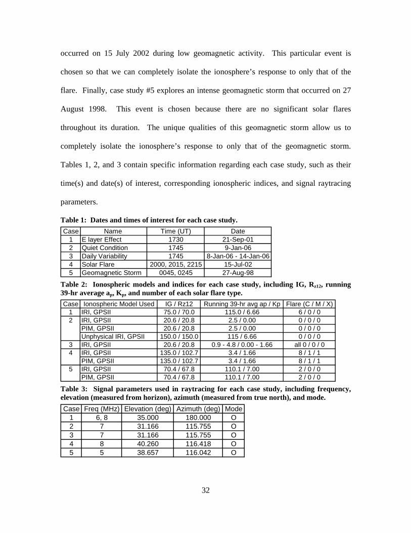
1. Dates and times of interest for each case study. .......................................................... 32

2. Ionospheric models and indices for each case study (IG, Rz12, ap, Kp, flare type #).... 32

3. Parameters used in raytracing for each case study (freq, elev, azimuth, mode) .......... 32

xi

ASSESSMENT OF THE IMPACT OF VARIOUS IONOSPHERIC MODELS

ON HIGH-FREQUENCY SIGNAL RAYTRACING

Introduction

Motivation

The ionosphere affects a wide array of current Department of Defense (DoD)

missions. For example, the ability to communicate with satellites relies on

electromagnetic signals successfully propagating through the ionosphere without

excessive attenuation or refraction. Furthermore, high-frequency (HF) communications,

over-the-horizon RADAR (OTHR), and certain methods of target direction finding all

require electromagnetic signals to be refracted within the ionosphere. Future combat

operations will continue to rely on our ability to precisely and accurately locate an

enemy’s position. Active sensing techniques can regrettably reveal the locations of

friendly forces. This research focuses on the goal of developing an ability to geo-locate

an enemy solely through intercepted communications. Even better, perform this geo-

location passively without revealing the location of friendly forces. The future success of

geo-location, as well as the other DoD missions, remains highly dependent on our ability

to accurately measure and predict the dynamic state of the ionosphere.

One of the most recent advances in ionospheric modeling is the NorthWest

Research Associates’ (NWRA) Global Positioning System (GPS) Ionospheric Inversion

(GPSII) model. As its name suggests, the model employs real-time Total Electron

Content (TEC) information that is passively obtained from GPS signals. Two additional

1

ionospheric models currently available are the 2001 version of the International

Reference Ionosphere (IRI-2001) model and the Parameterized Ionospheric Model (PIM).

This thesis will focus on assessing the impact of these ionospheric models on HF signal

raytracing when applied to the critical national defense mission of geo-location.

For the purpose of this thesis, geo-location describes the act of locating and/or

tracking an enemy using HF signals. The two main techniques of geo-location use either

multiple receiver sites or a single receiver site. This thesis focuses on a rigorous version

of the latter technique, commonly referred to as “single site location” (SSL), which uses a

complex three-dimensional raytracing algorithm and an ionospheric model to predict a

signal’s propagation path.

Ionospheric refraction can greatly affect the propagation behavior of a signal,

especially in the HF range of frequencies. If the state of the ionosphere is not properly

specified, the raytracing algorithm will produce an erroneous enemy location. The

primary objective of this thesis is to assess the impact of the three ionospheric models on

HF signal raytracing during various ionospheric conditions. The secondary objective is

to determine whether using passive techniques to model the ionosphere is sufficiently

accurate for geo-location. Categorizing the models’ strengths and weaknesses will

improve our ability to locate an enemy and, in turn, enhance the first four stages of the

Air Force’s six-stage “kill chain”, which is find, fix, track, and target.

Overview

This thesis includes a comparison of high-frequency (HF) signal raytracing using

the 2001 version of the International Reference Ionosphere (IRI-2001) model, the

Parameterized Ionospheric Model (PIM), and the new Global Positioning System (GPS)

2

Ionospheric Inversion (GPSII) model. These comparisons are done for various

ionospheric conditions, including: quiet, daily variability, solar flare, and geomagnetic

storming. Model strengths and weaknesses are discussed, as well as whether using

passive techniques to model the ionosphere is sufficiently accurate for geo-location.

Chapter two describes important background knowledge: the ionospheric

environment (structure and behavior), signal propagation, ionospheric models, geo-

location, and raytracing. Chapter three discusses the methodology used for this thesis,

which is mostly the procedures for properly integrating the three main components of

data collection, processing, and visualization: the ionospheric model, raytracing

algorithm, and MATLAB® software. Chapter four presents the case study results, while

chapter five provides conclusions and recommendations for future research.

Results Preview

The case studies reveal many interesting characteristics of the ionospheric models

when applied to HF signal raytracing. It is shown that the ionosphere’s E layer by itself

can increase a signal’s ground range by over 100 km, stressing the importance of

accurately specifying the lower ionosphere. It is also shown that the GPSII model has the

potential to capture the expected daily variability of the ionosphere by using TEC data,

which can affect a signal’s ground range by as much as 5 km per day. Furthermore, the

GPSII model can capture the upper-ionospheric response to both a solar flare and a

geomagnetic storm, yet cannot capture the lower-ionospheric response to either event.

These results suggest that using the GPSII model’s passive technique by itself may only

be beneficial to specifying the ionosphere above the E region, especially during solar

flares and geomagnetic storms.

3

Background

Ionospheric Environment

The ionosphere is defined as the ionized region of the Earth’s upper atmosphere,

comprised of several layers containing free electrons and various ionized particles. Solar

photons provide the primary source of ionization, as extreme ultraviolet (EUV) and x-ray

radiation break apart neutral atmospheric molecules to produce ions and free electrons.

Secondary sources of ionization are photoelectrons, energetic particle precipitation,

auroral precipitation, scattered radiation, starlight, and meteors. The mid-latitude

ionosphere, in which this thesis will focus, is composed of the following layers: D, E, F1,

F2, and the topside ionosphere. It is typically accepted that the ionosphere begins at

around 60 kilometers (km) and extends to approximately 1000 km, depending on the

degree of solar activity. The ionosphere transitions to the plasmasphere above 1000 km.

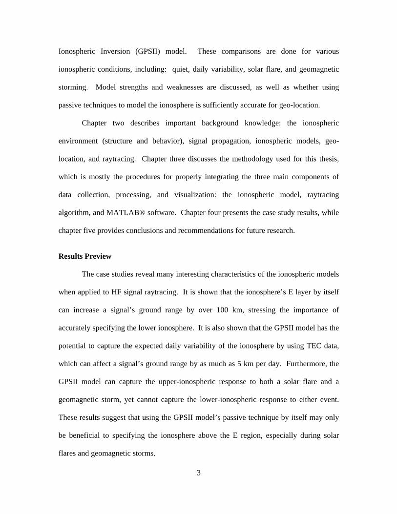
Davies [1989] provides a good illustration of the ionospheric regions, reproduced in

Figure 1. Each layer can be distinguished by a local peak in the electron density profile

corresponding to a particular dominating ion species. In addition, each layer is controlled

by different production and loss mechanisms with varying reaction rates. The remainder

of this section will briefly describe each layer and their relevant temporal behavior.

The D region (60 to 90 km) is dominated by photochemical processes and has the

most diverse composition, including: molecular ions, positive and negative ions, and

water cluster ions. Consequently, this region is considered to be the most difficult to

model and observe with any reliability [Schunk and Nagy, 2000]. The E region (90 to

150 km) is also dominated by photochemistry and consists primarily of molecular ions

such as O2+, N2

+, and NO+ that form an observable peak in the density profile. The F1

4

region (150 to 250 km) is still dominated by photochemical processes, yet is the

transition region in which O+ becomes the principal ion species. Although not dominant,

there are also transport mechanisms present in this region, such as ambipolar diffusion,

wind-induced drifts along magnetic field lines, and electrodynamic drifts across magnetic

field lines [Schunk and Nagy, 2000]. The F2 region (250 to 450 km) is where the

importance of these transport mechanisms become balanced with the photochemical

processes, creating a well-defined peak in the O+ density profile. The topside ionosphere

is the region above the F2 peak where the transport mechanisms dominate, resulting in an

exponential decrease in O+ density with altitude. Given that this thesis focuses on geo-

location, we are only interested in the ionosphere’s behavior below the F2 peak where

maximum refraction of HF signals occurs.

Figure 1: Ionosphere electron density (m-3) as a function of altitude (km) depicting the typical ionospheric layers observed on a mid-latitude summer day. The main bands of solar and cosmic ionizing radiation are noted [Davies, 1989].

5

One of the main techniques for obtaining real-time observations of the ionosphere

below the F2 peak uses vertical incidence ionosondes, which are HF radars that are

directed toward zenith. A sweep of frequencies is transmitted and the time delay of each

signal’s return is measured. The following expression relates the plasma frequency pf of

a layer (in MHz) to the electron density (in meN -3) [Sturrock, 1994].

( ) 6MHz 9 10 (m )pf −× -3eN (1)

Ignoring the effect of the Earth’s magnetic field, the critical frequency cf of the

ionosphere is the maximum frequency that can be still be refracted back to the ground

when transmitted toward zenith. Signals with frequencies higher than the critical

frequency will pass through the ionosphere. A signal’s “virtual height of reflection” is

equivalent to the distance that the signal would have traveled during half the elapsed

travel time, assuming it traveled at the speed of light in free space. An ionogram is a plot

of this virtual height as a function of frequency; an example is shown in Figure 2. In this

figure, the solid black line is the plasma frequency (which equates to electron density via

Equation 1) as a function of height, found by inverting the observed virtual height. Note

that ionosondes can only determine the “bottomside” frequency profile of the ionosphere;

models are used to estimate the “topside” profile. Estimates of the electron density can

be used to determine the ionosphere’s refractive index as a function of position, which is

needed for raytracing.

The mid-latitude ionosphere exhibits dramatic changes on many timescales,

including diurnal, seasonal, solar cycle, and irregular variations. A good example of the

diurnal variation is seen in Figure 3, where the plasma frequency ( p ef N∝ ) is shown

6

Figure 2: A real-time ionogram created from a vertical incident ionosonde in Juliusruh on 15 April 2006 by the Leibniz-Institute of Atmospheric Physics. The transmitter emits a sweep of frequencies, the receiver detects the refracted signals, and then a “virtual height of reflection” is calculated from the signals’ travel time. The black line is the electron density profile computed from the virtual height. Colors denote strength of signal return (warm colors = stronger dB). The ionosphere above the F2 peak cannot be measured from a vertical sounding, thus models are used to estimate this.

as a function of height at Wright-Patterson Air Force Base (WPAFB) throughout an

entire day. The plasma frequency increases rapidly at sunrise (~ 1200 UT) due to

photoionization and then decays after sunset (~ 2100 UT) when photoionization vanishes.

In particular, notice how quickly the E layer decays after sunset. The rate of ionization is

strongly dependent on solar zenith angle at altitudes where photochemical processes

dominate, i.e. below the F2 peak. The electron density above the F2 peak is dependent not

only on solar zenith angle, but also transport processes such as the magnitude of

meridional neutral winds [Schunk and Nagy, 2000].

7

Figure 3: An example of the ionosphere’s diurnal variation. Plasma frequency (MHz) as a function of height (km) at Wright-Patterson AFB on the autumnal equinox during normal solar and geomagnetic activity.

Considering that photoionization is the main source of ionization, it is logical that

the ionosphere would display a strong seasonal variation as the solar zenith angle and

hence photon flux changes throughout the year. Figure 4 gives an example of the

seasonal variation in plasma frequency as a function of height at WPAFB at local noon.

Notice that the plasma frequency is greater in winter than in summer, in spite of the fact

that the solar zenith angle is greater in winter. This “seasonal anomaly” is due to the

ionosphere’s strong coupling with the neutral atmosphere, which also experiences

seasonal fluctuations. An increased O/N2 ratio in winter leads to a sufficient increase in

the effective O+ production rate, counteracting the solar zenith angle effect [Schunk and

Nagy, 2000].

8

Figure 4: An example of the ionosphere’s seasonal variation. Plasma frequency (MHz) as a function of height (km) for Wright-Patterson AFB at local noon on the autumnal equinox and solstices during normal solar and geomagnetic activity.

As with seasons, the solar radiation flux also varies with solar cycle. Solar EUV

flux, which is the primary photon energy for photoionization, is significantly greater at

solar maximum compared to solar minimum. Figure 5 shows an example of the solar

cycle variation in plasma frequency as a function of height at WPAFB at local noon. The

higher plasma frequencies (i.e. greater electron densities) at solar maximum are a result

of changes in the neutral atmosphere as well as greater solar radiation flux amplifying the

ionization rates.

9

Figure 5: An example of the ionosphere’s solar cycle variation. Plasma frequency (MHz) as a function of height (km) for Wright-Patterson AFB at local noon on the autumnal equinox during normal geomagnetic activity.

Irregular variations of the ionosphere include localized enhancements of the E

region, known as a sporadic E layer. This layer can be flat and homogeneous or rather

diffuse in size. An example of a sporadic E layer is seen in Figure 6. The electron

density is plotted as a function of altitude and time, as measured by the Arecibo

incoherent scatter radar [Schunk and Nagy, 2000]. There is a distinct sporadic E layer at

116 km, with a peak electron density of about 5 x 105 cm-3. This layer persists after

sunset (approximately 1800 local time) whereas the remainder of the region below the F2

peak quickly decays. Since zonal neutral winds induce vertical ion drifts, any vertical

wind shear will cause sporadic E layers to form where the drifts converge. Also seen in

10

Figure 6 is an “intermediate layer”, which can appear in the lower F region at night (in

this case 2030 local time) and gradually descends into the E region. In contrast to

sporadic E layers, this layer is primarily formed by convergence of vertical ion drifts due

to vertical wind shear of meridional rather than zonal neutral winds [Schunk and Nagy,

2000].

Figure 6: Ionospheric irregular variations. Electron density is shown as a function of both height and time. A sporadic E layer persists for the entire time period, while an intermediate layer begins to descend in height at approx 2000 LT. Density measured with Arecibo incoherent scatter radar on 7 May 1983. [Schunk and Nagy, 2000]

Another irregular variation of the ionosphere occurs during geomagnetic storms.

In particular, the F region experiences a density enhancement during the initial (or

positive) phase and then depletion during the main (or negative) phase of a geomagnetic

storm. The cause of this effect is still not well understood. Although beyond the scope

of this thesis, it is worth mentioning that the current hypothesis considers a combination

of three mechanisms. First, variations in the neutral wind will raise or lower the

11

ionosphere, thereby changing the neutral atom/molecule ratios and thus the ion

production/loss ratios. Second, the protonosphere’s ability to act as a reservoir and

“refill” the ionosphere at night is reduced during a geomagnetic storm. Third, heating

from the magnetosphere via O+ precipitation from the ring current increases the

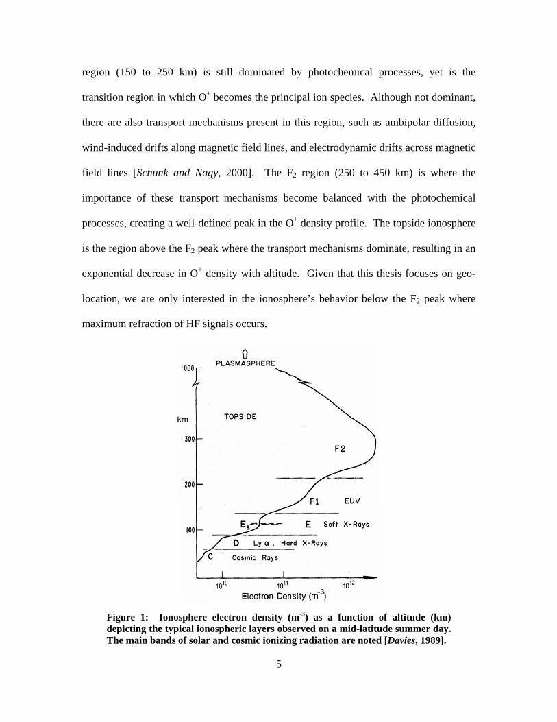
recombination rate [Hargreaves, 1992]. Figure 7 shows an example of the geomagnetic

storm variation in plasma frequency as a function of height at WPAFB at local noon.

The F region’s plasma frequency decreases as the geomagnetic storm strength increases,

characterized here by an increase in the 39-hr running average ap index. The ap index is

Figure 7: An example of the ionosphere’s variation during the main (or negative) phase of a geomagnetic storm. Plasma frequency (MHz) as a function of height (km) for Wright-Patterson AFB at local noon on the autumnal equinox during normal solar activity. Note that the E layer peak at approx. 110 km is the result of an oversimplification in the IRI “storming” model and is not a realistic response of the lower ionosphere during storming conditions.

12

the linear equivalent to the Kp index, which is a quasi-logarithmic index of the 3-hourly

range in magnetic field strength relative to a designated quiet-day curve, averaged and

standardized for 13 mid-latitude geomagnetic observatories. Note that Figure 7 is created

with the IRI-2001 model, which oversimplifies this effect by using a density scale factor

above 165 km. The model is then forced to interpolate below 165 km, creating an

unrealistic E layer at 110 km. A more detailed description of the IRI-2001 model will be

given in a subsequent background section titled “Ionospheric Models”.

Irregular variations in the ionosphere, such as sporadic E layers and F layer

depletion during geomagnetic storms, can make accurate raytracing of HF signals

considerably more difficult (if not impossible) due to their erratic behavior. The next

section describes a few of the most important ionospheric effects on HF signal

propagation.

Signal Propagation

Historic studies of HF signal propagation have revealed a wide range of

interesting and now well-documented ionospheric effects, such as absorption, frequency

shift, polarization shift, Faraday rotation, phase delay, group delay, and refraction. The

latter effect has been identified as having the greatest influence on geo-location accuracy

and therefore will be the focus of this section [McNamara, 1991]. We will see how

refraction is directly proportional to electron density and how it affects signal

propagation.

For simplicity, assume the signal is propagating within a cold, un-magnetized,

plasma. Based on the development of Sturrock [1994], the refractive index, n , for this

plasma is found to be the following:

13

2 2

2s

1 1plasma e

phase signal e ignal

q Ncnm

ων ω π υ

= = − = − 2 (2)

where is the speed of light, c phaseν the phase velocity, plasmaω the angular plasma

frequency, signalω the angular signal frequency, the electron density, q the electron

charge, the electron mass, and

eN

em signalυ the signal frequency. Equation 2 indicates that

the index of refraction approaches unity as the signal frequency approaches infinity or as

the electron density goes to zero. This is the point at which no refraction occurs and the

signal continues to propagate as it would in a vacuum. More importantly, the index of

refraction approaches zero as the signal frequency approaches the plasma frequency,

signifying the point at which the signal experiences maximum refraction.

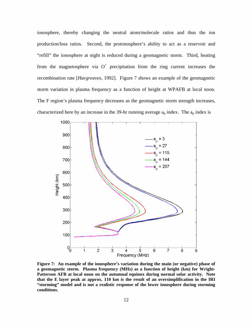
Akin to geometric optics, the propagation of a signal between two media of

differing refractive indices is given by Snell’s Law,

sin sini i rn n rθ θ= (3)

The subscripts differentiate between the incident (i) and refracting (r) medium, while the

angle θ is measured from the normal of the boundary. An illustration of this relation is

seen in Figure 8.

Figure 8: Snell’s Law. Electromagnetic wave refracts away from the boundary normal when traveling into medium with smaller refractive index (seen on right side).

14

As a fixed-frequency signal propagates from a higher to lower electron density the

refractive index of the plasma increases and the signal’s phase velocity decreases,

meaning the signal will refract toward the normal. Conversely, as the signal propagates

from a lower to higher electron density the refractive index of the plasma decreases and

the signal’s phase velocity increases, meaning the signal will refract away from the

normal. When conceptually applied to the ionosphere it is this latter case that ultimately

leads to signal “reflection”. If a signal is transmitted into an ideal ionosphere that can be

characterized as a horizontally homogeneous slab consisting of stratified layers of

increasing density (decreasing refractive index) with height, then Snell’s Law says that

the signal would eventually propagate perpendicular to the normal. It is at this point that

Snell’s Law breaks down, failing to explain how a signal is “reflected” by the ionosphere.

Therefore, the signal needs to be treated as a wave in order for the signal to continue

refraction back down to the original refractive index with the same angle of incidence, as

seen in Figure 9. A more detailed description of this wave treatment will be given in a

subsequent background section titled “Raytracing”.

Figure 9: Application of Snell’s Law in the ionosphere. The electromagnetic signal progressively refracts away from the boundary normal until the signal propagates perpendicular to the normal. Signal must be treated as a wave to account for continued refraction. Notice that the refractive index decreases with altitude, while the electron density increases with altitude.

15

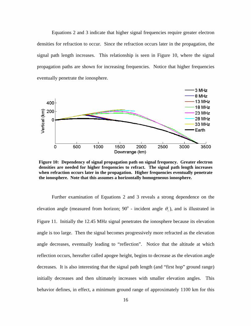
Equations 2 and 3 indicate that higher signal frequencies require greater electron

densities for refraction to occur. Since the refraction occurs later in the propagation, the

signal path length increases. This relationship is seen in Figure 10, where the signal

propagation paths are shown for increasing frequencies. Notice that higher frequencies

eventually penetrate the ionosphere.

Figure 10: Dependency of signal propagation path on signal frequency. Greater electron densities are needed for higher frequencies to refract. The signal path length increases when refraction occurs later in the propagation. Higher frequencies eventually penetrate the ionosphere. Note that this assumes a horizontally homogeneous ionosphere.

Further examination of Equations 2 and 3 reveals a strong dependence on the

elevation angle (measured from horizon; 90o - incident angle iθ ), and is illustrated in

Figure 11. Initially the 12.45 MHz signal penetrates the ionosphere because its elevation

angle is too large. Then the signal becomes progressively more refracted as the elevation

angle decreases, eventually leading to “reflection”. Notice that the altitude at which

reflection occurs, hereafter called apogee height, begins to decrease as the elevation angle

decreases. It is also interesting that the signal path length (and “first hop” ground range)

initially decreases and then ultimately increases with smaller elevation angles. This

behavior defines, in effect, a minimum ground range of approximately 1100 km for this

16

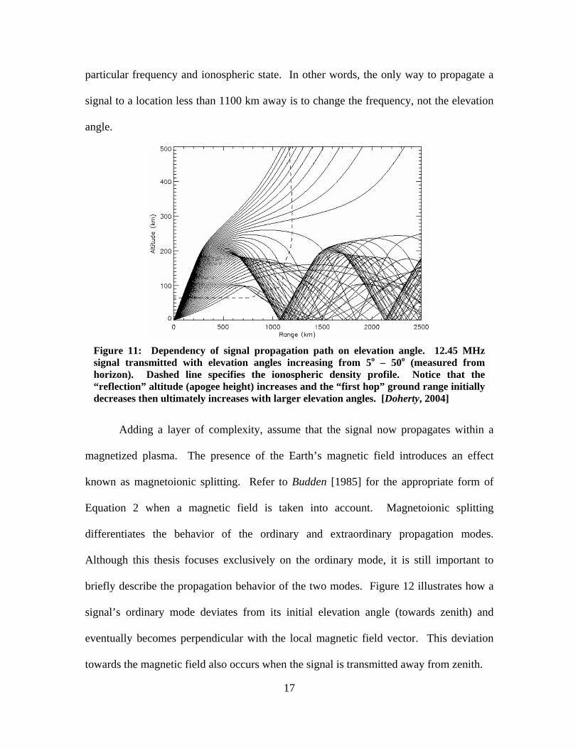
particular frequency and ionospheric state. In other words, the only way to propagate a

signal to a location less than 1100 km away is to change the frequency, not the elevation

angle.

Figure 11: Dependency of signal propagation path on elevation angle. 12.45 MHz signal transmitted with elevation angles increasing from 5o – 50o (measured from horizon). Dashed line specifies the ionospheric density profile. Notice that the “reflection” altitude (apogee height) increases and the “first hop” ground range initially decreases then ultimately increases with larger elevation angles. [Doherty, 2004]

Adding a layer of complexity, assume that the signal now propagates within a

magnetized plasma. The presence of the Earth’s magnetic field introduces an effect

known as magnetoionic splitting. Refer to Budden [1985] for the appropriate form of

Equation 2 when a magnetic field is taken into account. Magnetoionic splitting

differentiates the behavior of the ordinary and extraordinary propagation modes.

Although this thesis focuses exclusively on the ordinary mode, it is still important to

briefly describe the propagation behavior of the two modes. Figure 12 illustrates how a

signal’s ordinary mode deviates from its initial elevation angle (towards zenith) and

eventually becomes perpendicular with the local magnetic field vector. This deviation

towards the magnetic field also occurs when the signal is transmitted away from zenith.

17

Figure 12: Magnetoionic splitting of a 5 Hz signal transmitted toward zenith from Wright-Patterson AFB at local noon on the autumnal equinox during normal solar and geomagnetic activity. The signal’s propagation is affected by the local magnetic field. The signal’s ordinary mode refracts to become perpendicular to the local magnetic field vector, while its extraordinary mode refracts to become parallel.

Figure 13 shows the crossrange track of a signal transmitted towards magnetic

west as a function of distance downrange from the transmitter (i.e. propagation path

projected onto x-y plane; note axes scale difference). The signal’s ordinary mode begins

to deviate towards magnetic north as it enters the ionosphere, reaches maximum

crossrange at the point of “reflection”, and then returns to the original transmission

azimuth angle (measured from true north) as it exits the ionosphere. The same deviation

occurs for transmission towards magnetic east. The magnitude of this deviation

decreases as the transmission azimuth becomes more aligned with a magnetic meridian.

In other words, there is no deviation when the signal is transmitted parallel to a magnetic

meridian, such as from magnetic north to south or south to north. Both of these examples

simply illustrate how propagation behavior is dependent on a signal’s mode. Appendix A

contains additional examples of magnetoionic splitting behavior.

18

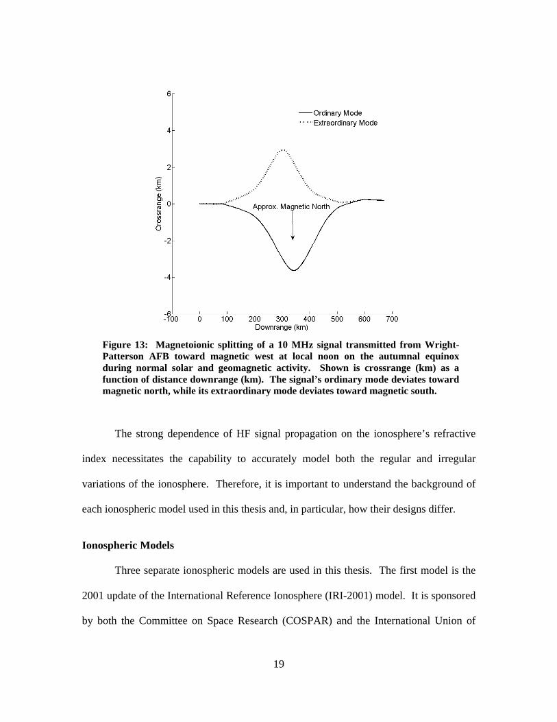
Figure 13: Magnetoionic splitting of a 10 MHz signal transmitted from Wright-Patterson AFB toward magnetic west at local noon on the autumnal equinox during normal solar and geomagnetic activity. Shown is crossrange (km) as a function of distance downrange (km). The signal’s ordinary mode deviates toward magnetic north, while its extraordinary mode deviates toward magnetic south.

The strong dependence of HF signal propagation on the ionosphere’s refractive

index necessitates the capability to accurately model both the regular and irregular

variations of the ionosphere. Therefore, it is important to understand the background of

each ionospheric model used in this thesis and, in particular, how their designs differ.

Ionospheric Models

Three separate ionospheric models are used in this thesis. The first model is the

2001 update of the International Reference Ionosphere (IRI-2001) model. It is sponsored

by both the Committee on Space Research (COSPAR) and the International Union of

19

Radio Science (URSI) and is often considered the standard for ionospheric parameters

[Bilitza, 2001]. Being an empirical climatology model, it determines the dominant

variations of ionospheric parameters from an existing observational database.

Experimental observations from all available data sources, including ground and space,

are used to predict a monthly average for each ionospheric parameter, assuming

magnetically quiet conditions in a non-auroral ionosphere. Several solar indices are used

as model input parameters. The 12-month running average of the sunspot number

produced at the Zurich observatory (Rz12) is used for the F peak altitude and topside

profile. Finally, the 39-hr running average of the ap index is used to capture the F region

depletion that occurs during a geomagnetic storm. IRI-2001 can also use real-time

ionosonde data for better representation of the E region. It is worth noting that a newer

version of IRI (after 2001) is being augmented to include TEC data inferred from GPS

satellite data as another real-time input. Of the many IRI-2001 output parameters, this

thesis only requires plasma frequency (i.e. electron density) as a function of position

within a user-specified 3-D grid.

The second model is the Parameterized Ionospheric Model (PIM). Unlike IRI-

2001, PIM is based on theoretical climatology rather than empirical climatology. While

empirical models are, by their very nature, limited by the quantity and type of observed

data, PIM produces a summary of the output of four physics-based numerical models

parameterized for a variety of ionospheric conditions. Daniell et al. [1995] provides a

concise description of the main difference between empirical and theoretical climatology:

Empirical climatology yields an “average” ionosphere in which the average may be taken over very different ionospheric configurations. Persistent features such as the subauroral trough, auroral oval, or equatorial anomaly may be smeared out or broadened as a result of the averaging process …

20

Theoretical climatology yields a “representative” ionosphere, i.e., an ionosphere that corresponds to a potentially realizable set of specific geophysical conditions. Ionospheric features will have locations, widths, amplitudes similar to those that might be observed on any given day under the specified geophysical conditions. Theoretical climatology is limited by the accuracy and completeness of the physics and chemistry included in the theoretical models on which it is based and the computer resources required to span the full range of geophysical conditions. [Daniell et al., 1995]

Parameterization is accomplished in a two-step process. First, the four physics-based

models created databases for distinct ionospheric conditions, such as various solar and

geomagnetic activity levels. Then these databases were fit with semi-analytic functions

to minimize storage space. PIM uses the Rz12 index to estimate solar activity and the Kp

index to estimate geomagnetic activity. For the purpose of this thesis, PIM’s 3-D grid

output of electron density is transformed into a 3-D grid of plasma frequency by using the

relation found in Equation 1.

The third model is the new GPSII model introduced in Chapter I. Ionosondes can

often be unavailable in a region of interest or their coverage may be too sparse to obtain

an accurate specification of the ionosphere, especially in a combat environment. The

GPSII model solves this problem by using passive measurements of the ionosphere. By

analyzing data collected from dual-frequency GPS ground receivers, the GPSII model

can estimate the TEC of the ionosphere along the many “lines of sight” between GPS

satellites and ground receivers. (One TEC unit (TECU) = 1016 electrons per square meter

integrated along the signal path.) Relative (or differential) TEC values are estimated by

differencing the phase between the L1-band (1575.42 MHz) and L2-band (1227.6 MHz)

GPS signals, while the absolute TEC data is estimated by differencing the group delay

between the two signals. In order to correct for inherent error found in the data, the

GPSII model accumulates statistics of both the GPS transmitter bias and receiver bias.

21

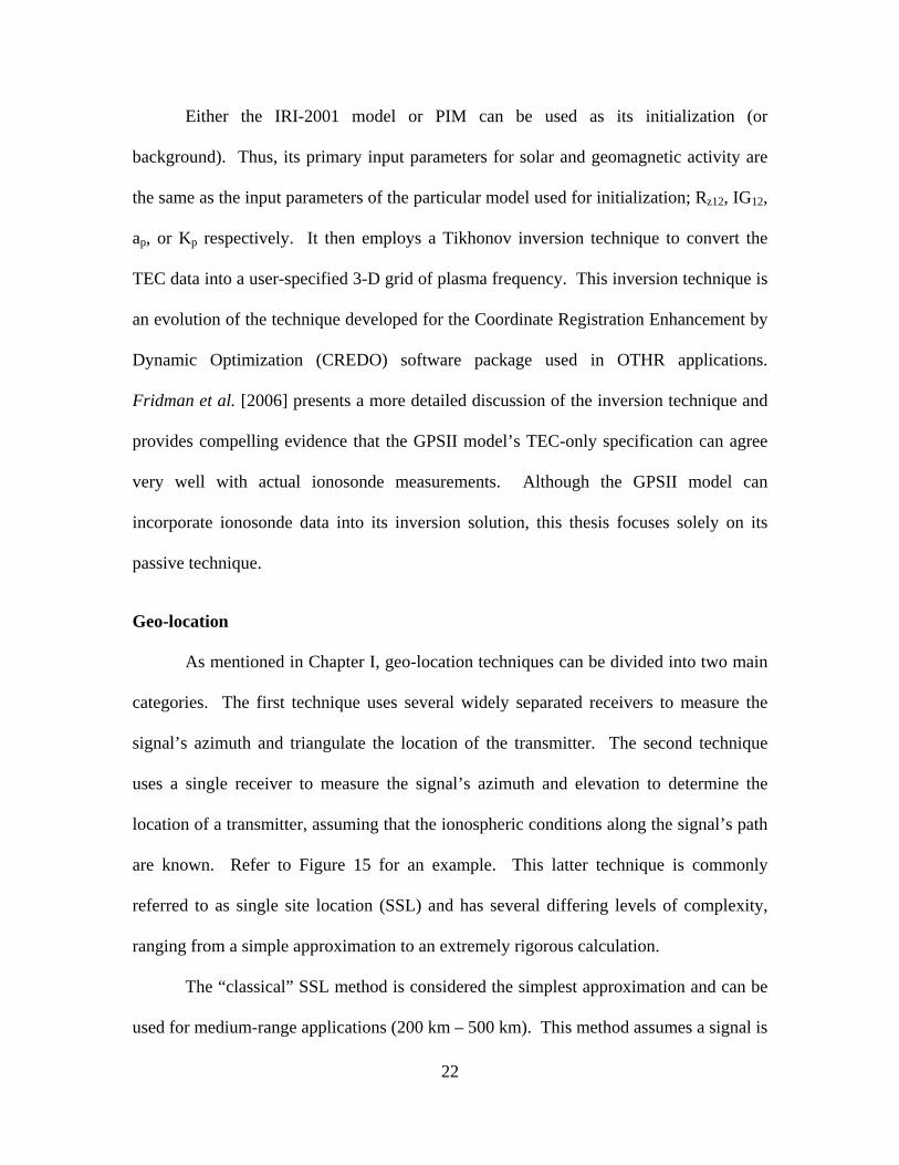
Either the IRI-2001 model or PIM can be used as its initialization (or

background). Thus, its primary input parameters for solar and geomagnetic activity are

the same as the input parameters of the particular model used for initialization; Rz12, IG12,

ap, or Kp respectively. It then employs a Tikhonov inversion technique to convert the

TEC data into a user-specified 3-D grid of plasma frequency. This inversion technique is

an evolution of the technique developed for the Coordinate Registration Enhancement by

Dynamic Optimization (CREDO) software package used in OTHR applications.

Fridman et al. [2006] presents a more detailed discussion of the inversion technique and

provides compelling evidence that the GPSII model’s TEC-only specification can agree

very well with actual ionosonde measurements. Although the GPSII model can

incorporate ionosonde data into its inversion solution, this thesis focuses solely on its

passive technique.

Geo-location

As mentioned in Chapter I, geo-location techniques can be divided into two main

categories. The first technique uses several widely separated receivers to measure the

signal’s azimuth and triangulate the location of the transmitter. The second technique

uses a single receiver to measure the signal’s azimuth and elevation to determine the

location of a transmitter, assuming that the ionospheric conditions along the signal’s path

are known. Refer to Figure 15 for an example. This latter technique is commonly

referred to as single site location (SSL) and has several differing levels of complexity,

ranging from a simple approximation to an extremely rigorous calculation.

The “classical” SSL method is considered the simplest approximation and can be

used for medium-range applications (200 km – 500 km). This method assumes a signal is

22

reflected from a simple horizontal mirror at a particular height, based on fundamental

laws of radio propagation in the ionosphere. The most important of these, conceptually,

is Martyn’s equivalent path theorem, which correlates a signal’s oblique reflection with

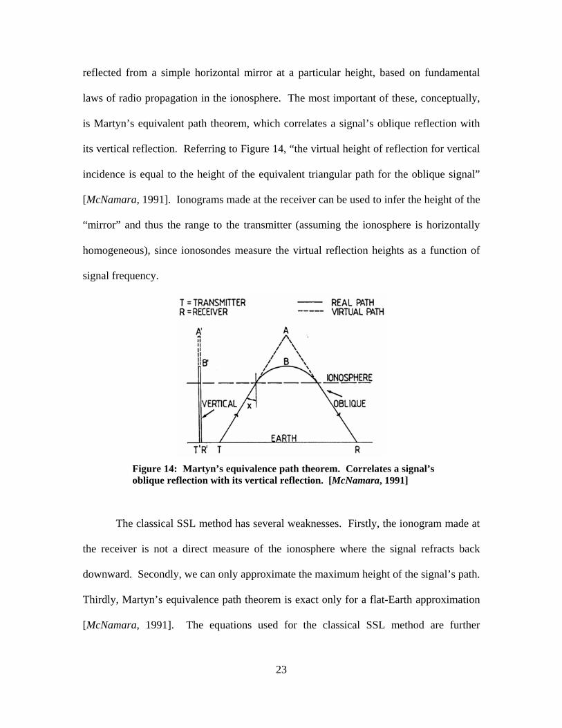
its vertical reflection. Referring to Figure 14, “the virtual height of reflection for vertical

incidence is equal to the height of the equivalent triangular path for the oblique signal”

[McNamara, 1991]. Ionograms made at the receiver can be used to infer the height of the

“mirror” and thus the range to the transmitter (assuming the ionosphere is horizontally

homogeneous), since ionosondes measure the virtual reflection heights as a function of

signal frequency.

Figure 14: Martyn’s equivalence path theorem. Correlates a signal’s oblique reflection with its vertical reflection. [McNamara, 1991]

The classical SSL method has several weaknesses. Firstly, the ionogram made at

the receiver is not a direct measure of the ionosphere where the signal refracts back

downward. Secondly, we can only approximate the maximum height of the signal’s path.

Thirdly, Martyn’s equivalence path theorem is exact only for a flat-Earth approximation

[McNamara, 1991]. The equations used for the classical SSL method are further

23

complicated when the presence of the Earth’s magnetic field is included. Refer to

McNamara [1991] for an example application of the classical SSL method.

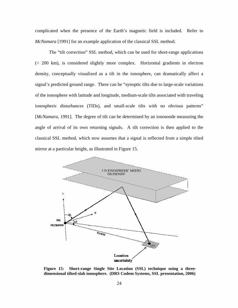
The “tilt correction” SSL method, which can be used for short-range applications

(< 200 km), is considered slightly more complex. Horizontal gradients in electron

density, conceptually visualized as a tilt in the ionosphere, can dramatically affect a

signal’s predicted ground range. There can be “synoptic tilts due to large-scale variations

of the ionosphere with latitude and longitude, medium-scale tilts associated with traveling

ionospheric disturbances (TIDs), and small-scale tilts with no obvious patterns”

[McNamara, 1991]. The degree of tilt can be determined by an ionosonde measuring the

angle of arrival of its own returning signals. A tilt correction is then applied to the

classical SSL method, which now assumes that a signal is reflected from a simple tilted

mirror at a particular height, as illustrated in Figure 15.

Figure 15: Short-range Single Site Location (SSL) technique using a three-dimensional tilted-slab ionosphere. (DRS Codem Systems, SSL presentation, 2006)

24

Raytracing, which can be used for long-range applications (> 500 km), is the most

rigorous SSL method. As emphasized in the next section, raytracing relies heavily on

having accurate knowledge of the ionosphere’s electron density profile along the entire

signal path. For that reason, a good ionospheric model becomes a crucial component.

There can be many levels of raytracing complexity, depending on the ionospheric

model’s accuracy and the method of computation. Methods range from analytic

raytracing with a simple one-dimensional non-magnetic ionosphere to numerical

raytracing through a complex three-dimensional magnetic ionosphere. The theory and

evolution of the numerical raytracing used in this thesis are presented in the next section.

Raytracing

The concepts found within geometrical optics eventually became the foundation

for raytracing theory. In his third treatise supplement on geometrical optics, Hamilton

[1832] introduced a set of differential equations that described the path of an

electromagnetic signal through an anisotropic medium. In the dawn of the computer age,

Haselgrove [1954] suggested that computers could numerically integrate Hamilton’s

equations and become “a new method for calculating ray paths in the ionosphere”.

Within a few years Haselgrove and her husband developed “a raytracing program to

calculate ‘twisted ray paths’ through a model ionosphere using Cartesian coordinates”

[Haselgrove and Haselgrove, 1960]. Further efforts came to fruition in 1975, when

Jones and Stephenson [1975] developed a FORTRAN program to calculate a signal’s

three-dimensional path through an ionosphere whose refractive index constantly varied.

We use an updated version of the Jones-Stephenson raytracing algorithm developed by

Mark Hausman and L.J. Nickisch of NWRA.

25

Hamilton’s differential equations have been derived using a variety of techniques

throughout the years. Typically the form of the equations is dependent on their

application, such as OTHR [Coleman, 1998] versus HF communications [McDonnell,

2000]. These equations are now collectively known as the “Haselgrove ray equation

system” and are used within the Jones-Stephenson raytracing algorithm [Huang and

Reinisch, 2006]. For the full derivation of these equations refer to Jones and Stephenson

[1975] or Nickisch [1988]. This system of equations becomes considerably more

complicated when the Earth’s magnetic field is included. For a thorough description of

propagation in the presence of a magnetic field refer to Kelso [1964], Davies [1989], or

Budden [1985].

The equation set emphasizes how the signal’s position and propagation vector are

dependent on the ionosphere’s index of refraction along the propagation path. The

equations are numerically integrated at each step along the signal’s propagation path,

resulting in a new position and propagation vector for the signal at each successive step.

The usefulness of this solution depends entirely on the accurate specification of the 3-D

refractive index. Theoretically, we can measure the electron density as a function of

position and then determine its refractive index by using Equation 2. However, it is

impractical (and perhaps impossible) to fully specify the ionosphere through

measurements alone, which is why ionospheric models are used to fill the gap.

Significant effort has been made by Hausman and Nickisch to ensure the

raytracing algorithm works well with the models [Fridman et al., 2006]. As a

consequence of design, successful synthesis of the raytracing algorithm and the

ionospheric models, especially when doing comparison studies, requires a disciplined

26

organizational structure. Furthermore, the visualization of the output depends upon

software such as MATLAB®, as well as considerable programming experience. The

next chapter describes the methods used to connect each of these components, as well as

the reasons for particular case study selections.

27

Methodology

Overview

The primary objective of this thesis is to assess the impact of the three ionospheric

models on HF signal raytracing during various ionospheric conditions. The secondary

objective is to determine whether using passive techniques to model the ionosphere is

sufficiently accurate for geo-location. Achieving these objectives require the integration

of the ionospheric models, the Hausman – Nickisch update of the Jones – Stephenson

raytracing algorithm, and MATLAB®. Figure 16 provides a summary of the flow of data

between the components and the user.

Figure 16: Summary of the flow of data between the user and the required components. The user directs the components to read initialization parameters, process data, and output results in proper formats for visualization and comparison.

This process is similar to that used by Aune [2006] in his study of trans-ionospheric

raytracing. Each component requires interface with the user at various stages of the

process. First, GPS data is collected for a user-defined region of interest using

MATLAB®. Once initialized with user-defined parameters, the GPSII model produces

28

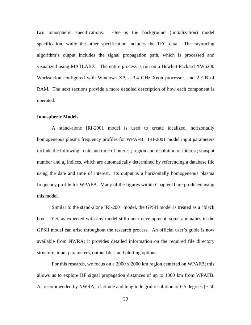
two ionospheric specifications. One is the background (initialization) model

specification, while the other specification includes the TEC data. The raytracing

algorithm’s output includes the signal propagation path, which is processed and

visualized using MATLAB®. The entire process is run on a Hewlett-Packard XW6200

Workstation configured with Windows XP, a 3.4 GHz Xeon processor, and 2 GB of

RAM. The next sections provide a more detailed description of how each component is

operated.

Ionospheric Models

A stand-alone IRI-2001 model is used to create idealized, horizontally

homogeneous plasma frequency profiles for WPAFB. IRI-2001 model input parameters

include the following: date and time of interest; region and resolution of interest; sunspot

number and ap indices, which are automatically determined by referencing a database file

using the date and time of interest. Its output is a horizontally homogeneous plasma

frequency profile for WPAFB. Many of the figures within Chapter II are produced using

this model.

Similar to the stand-alone IRI-2001 model, the GPSII model is treated as a “black

box”. Yet, as expected with any model still under development, some anomalies in the

GPSII model can arise throughout the research process. An official user’s guide is now

available from NWRA; it provides detailed information on the required file directory

structure, input parameters, output files, and plotting options.

For this research, we focus on a 2000 x 2000 km region centered on WPAFB; this

allows us to explore HF signal propagation distances of up to 1000 km from WPAFB.

As recommended by NWRA, a latitude and longitude grid resolution of 0.5 degrees (~ 50

29

km) is used. In addition, a stepped altitude grid is selected for maximum resolution

below the F2 peak. Bearing in mind the time scales of most ionospheric behaviors, a time

resolution of 15 minutes is adequate. The minimum distance between GPS ground

receivers is set to a value (~ 250 km) that results in a maximum of 21 receivers to be used

by the GPSII model. This upper limit on the number of used receivers is chosen in order

to avoid system crashes due to computer processor/memory limitations, whilst ensuring

sufficient TEC data availability. An example of GPSII input parameters are found in

Appendix B.

The GPSII model is ran with a time interval of at least 12 hours so as to collect

GPS satellite and ground receiver bias statistics for each particular day of interest. The

model is then run again with a time interval of 24 hours (0000 UT – 2400 UT) using the

previously collected bias statistics. Among its many output files are two ionospheric

specifications, i.e. 3-D grids of plasma frequency. The first specification is that of the

initialization model (either IRI-2001 or PIM), while the second includes the TEC data.

These ionospheric specifications are then used by the raytracing algorithm to determine

the propagation path of user-chosen HF signals.

Hausman – Nickisch Raytracing Algorithm

This update to the Jones-Stephenson raytracing algorithm is also treated as a

“black box”. Critical input parameters include the following: latitude/longitude of

transmitter (WPAFB); signal frequency, azimuth angle, elevation angle, and signal mode;

file name of 3-D plasma frequency grid. An example of these input parameters, as well

as many others, is shown in Appendix C. For additional guidance on the algorithm’s

operation, refer to the unofficial user’s guide written by Aune [2006] or to the official

30

user’s guide provided by NWRA. The raytracing code produces the 3-D position of the

HF signal along its entire propagation path, from the transmitter to where it impacts the

Earth’s surface (receiver). Note that the raytracing code can also calculate multiple hops

of a signal. This data is then ingested and visualized using MATLAB®.

Case Study Selection

Five case studies are used to assess the impact of various ionospheric models on

HF signal raytracing. These case studies cover an assortment of ionospheric conditions,

ranging from quiet conditions to solar flares and geomagnetic storms. Specific signal

frequencies are chosen in order to avoid ionospheric penetration, which is dependent on

the particular case study’s ionospheric conditions. This also holds true for a signal’s

elevation angle of transmission. As a reminder, this thesis examines only a signal’s

ordinary mode of propagation and not its extraordinary mode.

Case study #1 is chosen in an effort to isolate the effect that the E layer has on

signal propagation and geo-location. As described in the previous section, the stand-

alone IRI-2001 model is used to create an idealized, horizontally homogeneous

ionosphere. This ionosphere is then manually adjusted to have either a significant E layer

or no E layer at all. For our “base reference”, we design case study #2 to compare the

ionospheric models at local noon on a day with totally quiet solar and geomagnetic

conditions.

As for the remaining three case studies, our approach is to isolate certain

ionospheric drivers. For example, case study #3 focuses simply on the daily variability of

the ionosphere at local noon during seven consecutive days of very low solar and

geomagnetic activity. Meanwhile, case study #4 investigates a strong X3 solar flare that

31

occurred on 15 July 2002 during low geomagnetic activity. This particular event is

chosen so that we can completely isolate the ionosphere’s response to only that of the

flare. Finally, case study #5 explores an intense geomagnetic storm that occurred on 27

August 1998. This event is chosen because there are no significant solar flares

throughout its duration. The unique qualities of this geomagnetic storm allow us to

completely isolate the ionosphere’s response to only that of the geomagnetic storm.

Tables 1, 2, and 3 contain specific information regarding each case study, such as their

time(s) and date(s) of interest, corresponding ionospheric indices, and signal raytracing

parameters.

Table 1: Dates and times of interest for each case study. Case Name Time (UT) Date

1 E layer Effect 1730 21-Sep-012 Quiet Condition 1745 9-Jan-063 Daily Variability 1745 8-Jan-06 - 14-Jan-064 Solar Flare 2000, 2015, 2215 15-Jul-025 Geomagnetic Storm 0045, 0245 27-Aug-98

Table 2: Ionospheric models and indices for each case study, including IG, Rz12, running 39-hr average ap, Kp, and number of each solar flare type. Case Ionospheric Model Used IG / Rz12 Running 39-hr avg ap / Kp Flare (C / M / X)

1 IRI, GPSII 75.0 / 70.0 115.0 / 6.66 6 / 0 / 02 IRI, GPSII 20.6 / 20.8 2.5 / 0.00 0 / 0 / 0

PIM, GPSII 20.6 / 20.8 2.5 / 0.00 0 / 0 / 0Unphysical IRI, GPSII 150.0 / 150.0 115 / 6.66 0 / 0 / 0

3 IRI, GPSII 20.6 / 20.8 0.9 - 4.8 / 0.00 - 1.66 all 0 / 0 / 04 IRI, GPSII 135.0 / 102.7 3.4 / 1.66 8 / 1 / 1

PIM, GPSII 135.0 / 102.7 3.4 / 1.66 8 / 1 / 15 IRI, GPSII 70.4 / 67.8 110.1 / 7.00 2 / 0 / 0

PIM, GPSII 70.4 / 67.8 110.1 / 7.00 2 / 0 / 0 Table 3: Signal parameters used in raytracing for each case study, including frequency, elevation (measured from horizon), azimuth (measured from true north), and mode. Case Freq (MHz) Elevation (deg) Azimuth (deg) Mode

1 6, 8 35.000 180.000 O2 7 31.166 115.755 O3 7 31.166 115.755 O4 8 40.260 116.418 O5 5 38.657 116.042 O

32

Results

Case Study #1: E layer Effect

The first case study examines how the E layer affects HF signal propagation. As

described in the previous chapter, we create two horizontally homogeneous ionospheres;

identical above the E region, but differing significantly within the E region. One has a

strong E layer, while the other has no E layer. Refer to Table 2 for the various

ionospheric indices that are used to generate these. The plasma frequency profiles for

both cases are shown in Figure 17; the figure represents the ionosphere over WPAFB at

local noon.

Figure 17: E layer variation. Plasma frequency (MHz) as a function of height (km) for Wright-Patterson AFB at local noon on the autumnal equinox during fictitious solar and geomagnetic conditions.

33

We simulate the transmission of both a 6 MHz and 8 MHz signal through these

idealized ionospheres. Refer to Table 3 for the specific signal parameters that are used

for the raytracing. The resulting propagation paths, projected onto the x-z plane, are seen

in Figure 18 (top = 6 MHz, bottom = 8 MHz). The signals have a simple, quasi-parabolic

trajectory when the E layer is negligible. Their trajectories become more complex when

a non-negligible E layer is added. The signals begin to refract earlier in their propagation

as they encounter the higher plasma frequencies of the E layer. They continue

propagating through the E layer and eventually refract back toward Earth due to the F

layer. Notice that the maximum height of their propagation path is exactly the same,

irrespective of E layer magnitude. This is because the two ionospheres have the same

plasma frequencies above 165 km, where the majority of the refraction occurs. The

signals are refracted again by the E layer as they return to the Earth’s surface. The

resulting “wavy” trajectories seen in Figure 18 are thus due to the presence of the E layer.

More importantly, the signals’ ground ranges increase by this effect because the

refractions occur earlier in their propagation. The ground range of the 6 MHz signal

increases by 165 km, while the ground range of the 8 MHz signal increases by 47 km.

The increase is less for the 8 MHz signal because its frequency is higher relative to the

plasma frequency of the E layer.

The upper and lower limits of this “E layer effect” can be found by increasing or

decreasing the signal frequency. Lowering the frequency increases the ground range

until the frequency becomes low enough to be “reflected” by the E layer. Raising the

frequency decreases the ground range offset until it eventually matches the negligible E

layer case (assuming that the higher frequency does not penetrate the F layer).

34

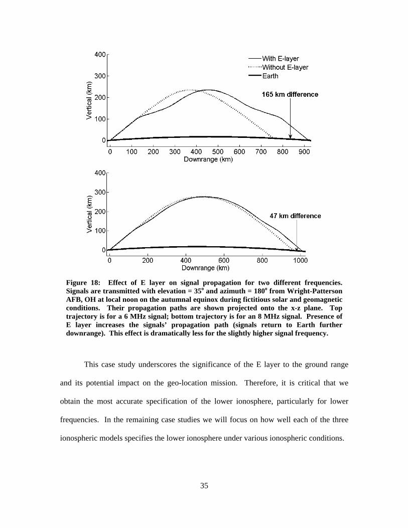
Figure 18: Effect of E layer on signal propagation for two different frequencies. Signals are transmitted with elevation = 35o and azimuth = 180o from Wright-Patterson AFB, OH at local noon on the autumnal equinox during fictitious solar and geomagnetic conditions. Their propagation paths are shown projected onto the x-z plane. Top trajectory is for a 6 MHz signal; bottom trajectory is for an 8 MHz signal. Presence of E layer increases the signals’ propagation path (signals return to Earth further downrange). This effect is dramatically less for the slightly higher signal frequency.

This case study underscores the significance of the E layer to the ground range

and its potential impact on the geo-location mission. Therefore, it is critical that we

obtain the most accurate specification of the lower ionosphere, particularly for lower

frequencies. In the remaining case studies we will focus on how well each of the three

ionospheric models specifies the lower ionosphere under various ionospheric conditions.

35

Case Study #2: Quiet Conditions

The second case study establishes a “base reference” by comparing the three

ionospheric models, and corresponding raytrace results, for quiet solar and geomagnetic

conditions. Local noon on 9 Jan 06 is selected to represent our quiet conditions. Refer to

Table 2 for the various ionospheric indices that describe this day. Figure 19 shows the

critical frequency contours (MHz) for local noon on 9 Jan 06 using the various models.

The left column depicts the results of the initialization model (IRI-2001 or PIM). The

right column is the GPSII model, using the corresponding initialization from the left

column. The middle row represents IRI-2001 and GPSII model results when unphysical

initialization conditions are used (compared to the actual quiet conditions of 9 Jan 06).

The intention is to gauge how well the GPSII model uses the measured TEC data to

adjust for unphysical initialization. The triangles indicate the position of GPS ground

receivers used in the GPSII model specification, while the crosses show the position of

ionospheric pierce points (at 400 km) for each satellite-receiver path.

There is a distinctive, consistent pattern throughout all of the GPSII model critical

frequency contours. The inner regions of plots have the most ionospheric pierce points,

with the outer few degrees (latitude/longitude) of the plots lacking them entirely.

Therefore, the most TEC data-driven model adjustments occur in the center of the grid.

Consequently, the GPSII model reverts to the initialization model along the outer

boundary. This produces a subtle “bulls-eye” pattern, which was originally recognized

and described by Fridman et al. [2006].

The critical frequency contours of the IRI-2001 model (top left) and PIM (bottom

left) initialization are remarkably similar. The GPSII model with IRI initialization (top

36

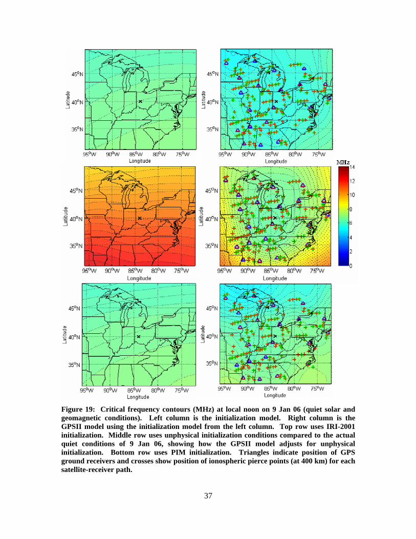
Figure 19: Critical frequency contours (MHz) at local noon on 9 Jan 06 (quiet solar and geomagnetic conditions). Left column is the initialization model. Right column is the GPSII model using the initialization model from the left column. Top row uses IRI-2001 initialization. Middle row uses unphysical initialization conditions compared to the actual quiet conditions of 9 Jan 06, showing how the GPSII model adjusts for unphysical initialization. Bottom row uses PIM initialization. Triangles indicate position of GPS ground receivers and crosses show position of ionospheric pierce points (at 400 km) for each satellite-receiver path.

37

right) has overall lower critical frequencies compared to the IRI-2001 model (top left) by

approximately 2 MHz. Meanwhile, the GPSII model with PIM initialization (bottom

right) only has these lower critical frequencies in the upper region of the plot compared to

PIM (bottom left). The two GPSII model specifications (top and bottom right) have

roughly the same contour pattern, disregarding the “boundary effect” described earlier.

A signal is transmitted from WPAFB toward Norfolk, VA in anticipation of

future ground truth data validation. Refer to Table 3 for the specific signal parameters

that are used for the raytracing. Figure 20 shows the plasma frequency profiles at the

signal’s approximate apogee for each of the six runs described in Figure 19.

Figure 20: Plasma frequency (MHz) as a function of height (km) at the approximate apogee of a signal transmitted from Wright-Patterson AFB, OH toward Norfolk, VA at local noon on 9 Jan 06 (quiet solar and geomagnetic conditions) using various ionospheric models. The IRI model representing unphysically active conditions compared to actual quiet conditions is shown in blue.

38

Examining Figure 20, it is interesting to note in regards to the topside ionosphere (above

the F2 peak) that the GPSII model makes significant adjustments to the IRI-2001 model

initialization, especially when the unphysical conditions are used (comparing black/blue

solid lines to dotted lines). In contrast, very little adjustment is made when the GPSII

model uses PIM for its initialization. In the lower ionosphere (below the F2 peak), the

GPSII model once again makes the least adjustment when it is initialized with PIM,

increasing the plasma frequency by no more than 0.25 MHz. All of the models have

relatively the same E region profiles. The unphysical IRI-2001 model has a slightly more

pronounced E layer in response to the higher indices that are used as its inputs.

Perhaps most interesting, the GPSII model does not make any significant

adjustments to the E layer, regardless of the initialization. This suggests that using TEC

data does not assist in specifying the E layer. A logical explanation of why TEC data

does not provide any E region information requires a closer look at the definition of TEC.

Vertical TEC (rather than slant TEC along the satellite/receiver path) is simply the

integration of the electron density with respect to altitude. Instead of the usual plasma

frequency profile, imagine a plasma density profile in linear coordinates. Remember

from Equation 1 that the plasma density is proportional to the square of its frequency.

The vertical TEC can then be represented as the integrated area to the left of the density

profile. Analyzed in this way, the contribution of the E region to vertical TEC is

considerably small and almost negligible. Therefore, it is extremely difficult, if not

impossible, to extract E region information from TEC measurements alone. Keeping this

in mind, it is doubtful that the GPSII model’s passive technique by itself can provide any

better specification of the E layer.

39

Figure 21 shows the resulting propagation path of an HF signal projected onto the

x-z plane for all model runs except the unphysical IRI-2001 model. Refer to Table 3 for

the specific signal parameters that are used for the raytracing. We find little difference

between the trajectory that is computed using PIM and the trajectory computed using the

GPSII model with PIM initialization (red lines). This is because there is very little

difference between the two ionospheric profiles, as mentioned earlier. There is a bigger

difference between the other two trajectories due to a larger divergence in their respective

ionospheric profiles below 175 km.

Figure 21: Propagation path projected onto the x-z plane for a 7 MHz signal transmitted from Wright-Patterson AFB, OH toward Norfolk, VA at local noon on 9 Jan 06 (quiet solar and geomagnetic conditions) using various ionospheric models.

The corresponding receiver locations are shown in Figure 22. A receiver location

is defined as the point where the signal impacts the Earth’s surface. The GPSII model

adjusts the receiver location by approximately 20 km from that of the IRI-2001

initialization and only 3 km from that of PIM initialization. Since the GPSII model uses

TEC data to create a more realistic specification of the ionosphere, we would expect to

see the receiver locations “converge” toward a common location, regardless of its

initialization. Instead, the receiver locations seen in Figure 22 actually “diverge” when

the GPSII model is used.

40

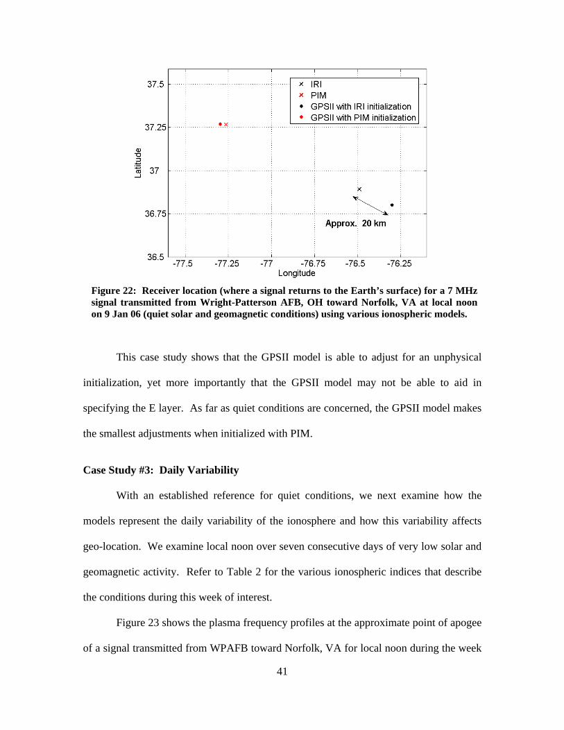
Figure 22: Receiver location (where a signal returns to the Earth’s surface) for a 7 MHz signal transmitted from Wright-Patterson AFB, OH toward Norfolk, VA at local noon on 9 Jan 06 (quiet solar and geomagnetic conditions) using various ionospheric models.

This case study shows that the GPSII model is able to adjust for an unphysical

initialization, yet more importantly that the GPSII model may not be able to aid in

specifying the E layer. As far as quiet conditions are concerned, the GPSII model makes

the smallest adjustments when initialized with PIM.

Case Study #3: Daily Variability

With an established reference for quiet conditions, we next examine how the

models represent the daily variability of the ionosphere and how this variability affects

geo-location. We examine local noon over seven consecutive days of very low solar and

geomagnetic activity. Refer to Table 2 for the various ionospheric indices that describe

the conditions during this week of interest.

Figure 23 shows the plasma frequency profiles at the approximate point of apogee

of a signal transmitted from WPAFB toward Norfolk, VA for local noon during the week

41

of interest using the IRI-2001 and GPSII models. The profiles of the IRI-2001 model are

tightly grouped and steadily decrease in plasma frequency throughout the week due to

changes in both the solar zenith angle and neutral atmosphere. In contrast, the profiles of

the GPSII model are erratic and have no trend in plasma frequency fluctuations,

especially in the lower ionosphere where maximum refraction of HF signals occurs (see

inset of Figure 23).

Figure 23: Plasma frequency (MHz) as a function of height (km) at the approximate apogee of a signal transmitted from Wright-Patterson AFB, OH toward Norfolk, VA at local noon during the week of 8 – 14 Jan 06 (very low solar and geomagnetic activity) using the IRI and GPSII models.

42

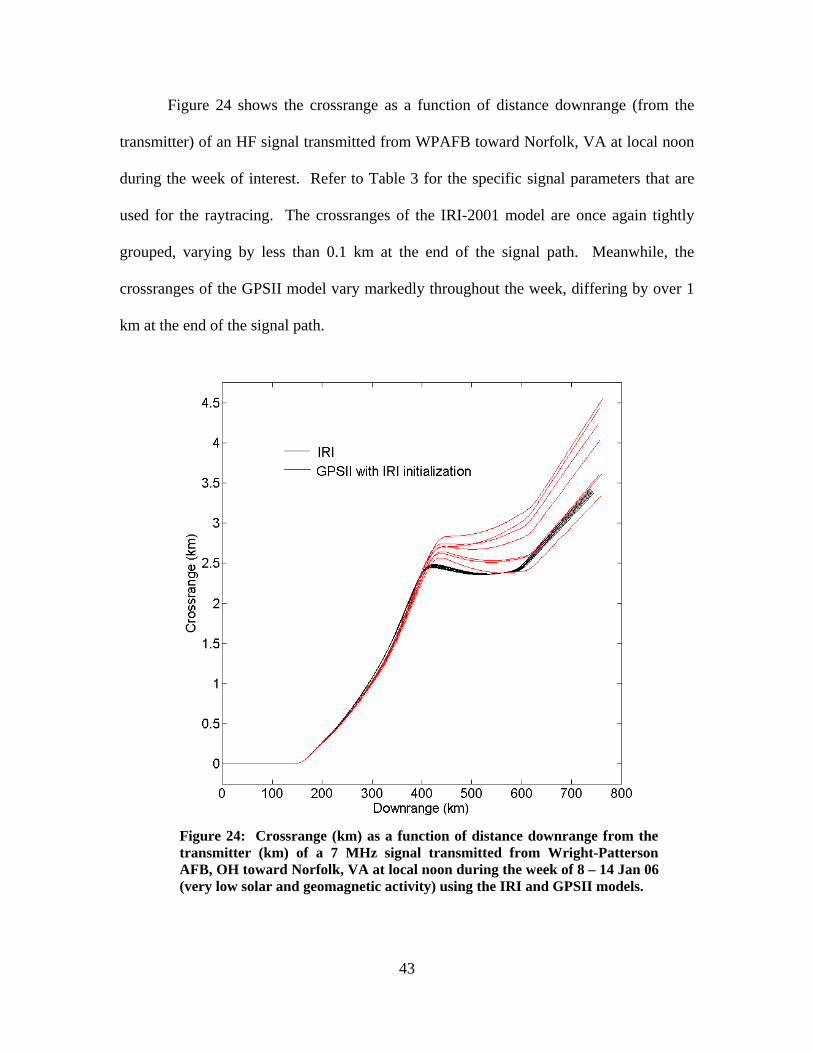
Figure 24 shows the crossrange as a function of distance downrange (from the

transmitter) of an HF signal transmitted from WPAFB toward Norfolk, VA at local noon

during the week of interest. Refer to Table 3 for the specific signal parameters that are

used for the raytracing. The crossranges of the IRI-2001 model are once again tightly

grouped, varying by less than 0.1 km at the end of the signal path. Meanwhile, the

crossranges of the GPSII model vary markedly throughout the week, differing by over 1

km at the end of the signal path.

Figure 24: Crossrange (km) as a function of distance downrange from the transmitter (km) of a 7 MHz signal transmitted from Wright-Patterson AFB, OH toward Norfolk, VA at local noon during the week of 8 – 14 Jan 06 (very low solar and geomagnetic activity) using the IRI and GPSII models.

43

The corresponding receiver locations are shown in Figure 25. The receiver

locations of the IRI-2001 model are shifted by a consistent 1 km step to the southeast

each day. This is due to the steady decrease in plasma frequency of the IRI-2001 model

throughout the week as the solar zenith angle decreases. In stark contrast, the receiver

locations of the GPSII model are highly variable, differing by as much as 5 km per day.

Figure 25: Receiver location (where a signal returns to the Earth’s surface) for a 7 MHz signal transmitted from Wright-Patterson AFB, OH toward Norfolk, VA at local noon during the week of 8 – 14 Jan 06 (very low solar and geomagnetic activity) using various ionospheric models.

These results show that the IRI model represents the daily variability of the

ionosphere as fairly steady, while the GPSII model represents the daily variability as

erratic. Furthermore, this daily variability has a considerable influence on the resulting

receiver location. We cannot make a firm conclusion of whether the GPSII model

captures the expected daily variability without comparison to ground truth data. In other

words, the model may just exhibit behavior that is characteristic of such real world

variability. Also keep in mind that these results are under quiet conditions. The daily

variability is even more pronounced during periods of high activity.

44

Case Study #4: Solar Flare Event

This case study completely isolates the ionosphere’s response to only that of a

solar flare. We examine a strong X3 solar flare that occurred on 15 July 2002 during low

geomagnetic activity. The flare began at approximately 2000 UT, reached a maximum at

approximately 2010 UT, and returned to background levels by 2215 UT. Refer to Table

2 for the various ionospheric indices that describe the conditions during this event. The

ionosphere’s characteristic response to a solar flare is an enhancement of the D and lower

E regions due to an increase in x-ray and EUV absorption. Since the IRI-2001 model and

PIM do not have input parameters to capture this increase in x-ray/EUV flux, our focus

turns to whether the GPSII model can capture the ionosphere’s response using the TEC

data.

Figure 26 shows the critical frequency contours during the solar flare event using

the GPSII model. Each row represents successive time steps of 2000 UT (flare

beginning), 2015 UT (5 minutes after flare maximum), and 2215 UT (return to

background levels). The left column is the GPSII model initialized with the IRI-2001

model, while the right column is the GPSII model initialized with PIM. The contours are

very similar at the beginning of the flare. An increase in the critical frequencies at 2015

UT (directly following the flare maximum) create a ridge in the contours that stretch into

Indiana, Ohio, and Michigan. The GPSII model has a more pronounced ridge when

initialized with PIM, including a maximum critical frequency centered over southern

Michigan. The ridge disappears by 2215 UT, returning the contours to roughly their

original shape and strength prior to the flare.

45

Figure 26: Critical frequency contours (MHz) during an X3 solar flare on 15 Jul 02. Left column is the GPSII model initialized with the IRI-2001 model. Right column is the GPSII model initialized with PIM. Each row represents successive time steps of before (2000 UT), during (2015 UT), and after the solar flare (2215 UT). Triangles indicate position of GPS ground receivers and crosses show position of ionospheric pierce points (at 400 km) for each satellite-receiver path.

46

The critical frequency contours only represent the strength of the F2 peak.

Therefore, we want to look at an entire plasma frequency profile for a location near the

contour ridge. Figure 27 shows the plasma frequency profiles for WPAFB at 2000 UT

and 2015 UT. As expected, the profiles of the IRI-2001 model and PIM do not change

between the two times. It is interesting that PIM has a stronger F1 region and upper E

region (from 125 km to 225 km) when compared to the IRI-2001 model. The GPSII

model makes the largest adjustments in plasma frequency in the upper ionosphere. This

is particularly true at 2015 UT when it is initialized with PIM, resulting in an

enhancement of the F1 region as well.

As in case study #2, the GPSII model does not make any adjustments to the E

layer, regardless of the initialization. We expect to see an increase in the lower E layer

plasma frequencies at the time of peak x-ray and EUV fluxes during the solar flare. This

ionization enhancement is due to absorption of the x-ray and EUV radiation. We can

surmise that the TEC data does not assist in specifying the E layer, since the GPSII model

does not show any of the expected enhancements. Remember from our earlier analysis of

TEC that the contribution of the E region to vertical TEC is more or less negligible,

making it exceedingly difficult to extract E region information from TEC data alone.

47

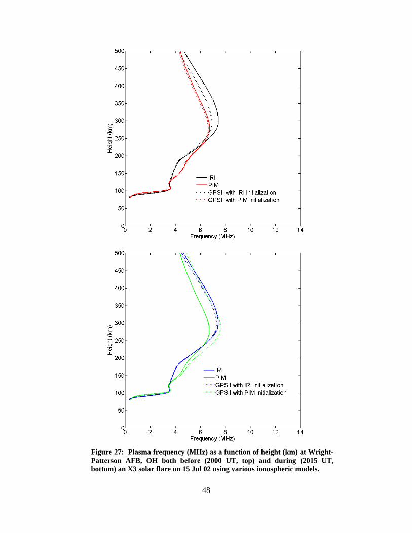
Figure 27: Plasma frequency (MHz) as a function of height (km) at Wright-Patterson AFB, OH both before (2000 UT, top) and during (2015 UT, bottom) an X3 solar flare on 15 Jul 02 using various ionospheric models.

48

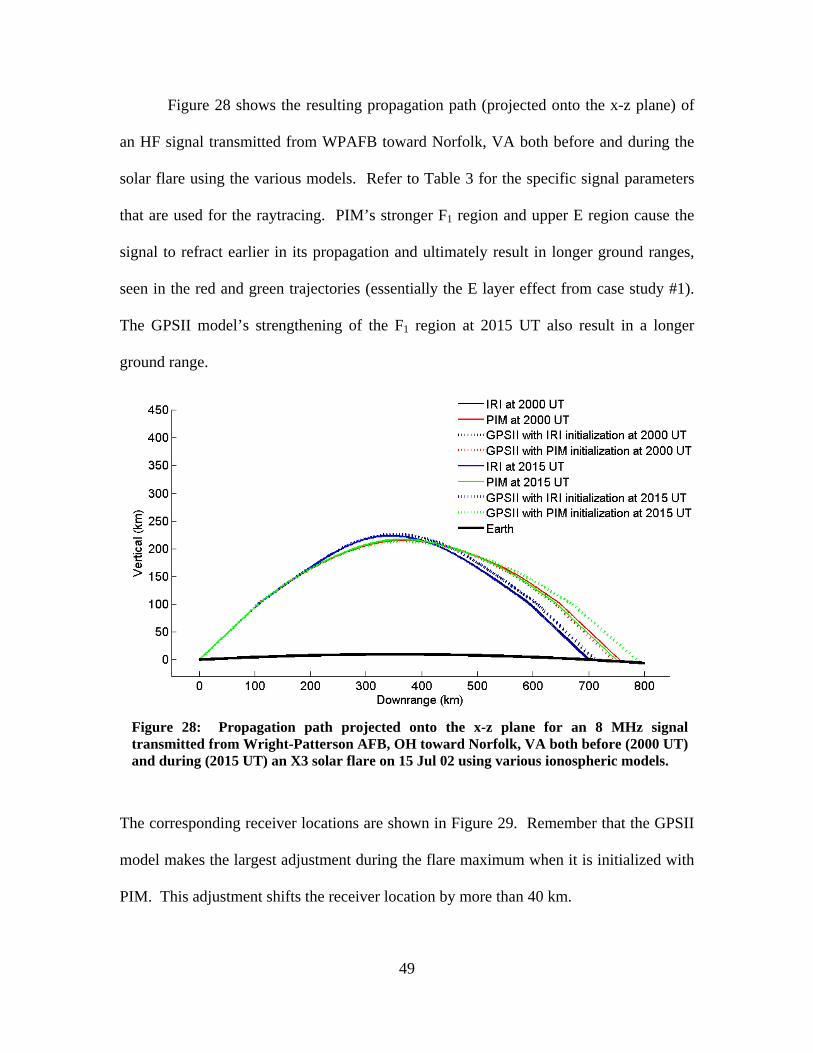
Figure 28 shows the resulting propagation path (projected onto the x-z plane) of

an HF signal transmitted from WPAFB toward Norfolk, VA both before and during the

solar flare using the various models. Refer to Table 3 for the specific signal parameters

that are used for the raytracing. PIM’s stronger F1 region and upper E region cause the

signal to refract earlier in its propagation and ultimately result in longer ground ranges,

seen in the red and green trajectories (essentially the E layer effect from case study #1).

The GPSII model’s strengthening of the F1 region at 2015 UT also result in a longer

ground range.

Figure 28: Propagation path projected onto the x-z plane for an 8 MHz signal transmitted from Wright-Patterson AFB, OH toward Norfolk, VA both before (2000 UT) and during (2015 UT) an X3 solar flare on 15 Jul 02 using various ionospheric models.

The corresponding receiver locations are shown in Figure 29. Remember that the GPSII

model makes the largest adjustment during the flare maximum when it is initialized with

PIM. This adjustment shifts the receiver location by more than 40 km.

49

Figure 29: Receiver location (where a signal returns to the Earth’s surface) for a signal transmitted from Wright-Patterson AFB, OH toward Norfolk, VA both before (2000 UT) and during (2015 UT) an X3 solar flare on 15 Jul 02 using various ionospheric models.

These results show that the IRI-2001 model and PIM can have significantly

different specifications of the lower ionosphere, especially the F1 and upper E regions.

The only way to determine which model has a better specification would be to compare

them to actual ionosonde data. More importantly, the GPSII model is able to capture the

upper-ionospheric response to a solar flare, yet not the lower-ionospheric response. The

TEC data once again does not aid in specifying the E layer. This suggests that using the

GPSII model’s passive technique by itself may not be sufficient, especially during solar

flares when the lower E region is noticeably enhanced. Therefore, active measuring

techniques may be necessary for proper specification of the E layer.

50

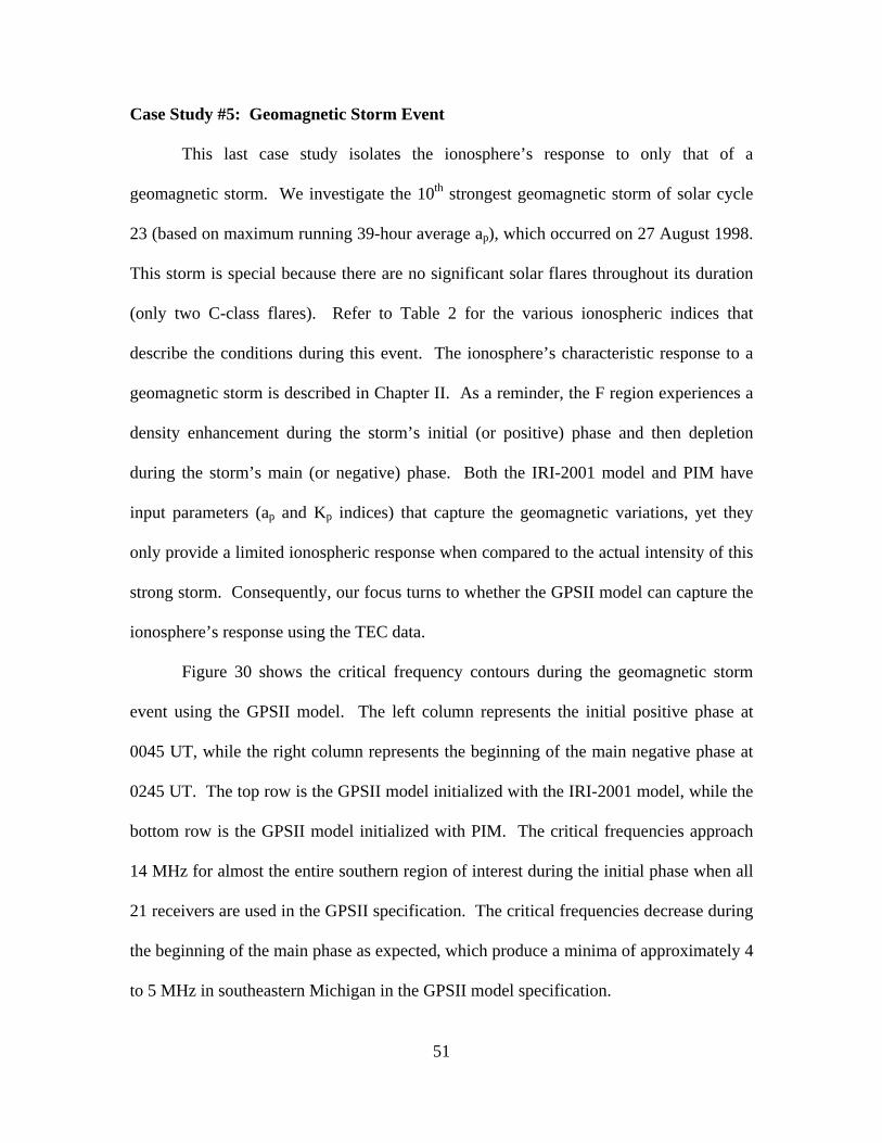
Case Study #5: Geomagnetic Storm Event

This last case study isolates the ionosphere’s response to only that of a

geomagnetic storm. We investigate the 10th strongest geomagnetic storm of solar cycle

23 (based on maximum running 39-hour average ap), which occurred on 27 August 1998.

This storm is special because there are no significant solar flares throughout its duration

(only two C-class flares). Refer to Table 2 for the various ionospheric indices that

describe the conditions during this event. The ionosphere’s characteristic response to a

geomagnetic storm is described in Chapter II. As a reminder, the F region experiences a

density enhancement during the storm’s initial (or positive) phase and then depletion

during the storm’s main (or negative) phase. Both the IRI-2001 model and PIM have

input parameters (ap and Kp indices) that capture the geomagnetic variations, yet they

only provide a limited ionospheric response when compared to the actual intensity of this

strong storm. Consequently, our focus turns to whether the GPSII model can capture the

ionosphere’s response using the TEC data.

Figure 30 shows the critical frequency contours during the geomagnetic storm

event using the GPSII model. The left column represents the initial positive phase at

0045 UT, while the right column represents the beginning of the main negative phase at

0245 UT. The top row is the GPSII model initialized with the IRI-2001 model, while the

bottom row is the GPSII model initialized with PIM. The critical frequencies approach

14 MHz for almost the entire southern region of interest during the initial phase when all

21 receivers are used in the GPSII specification. The critical frequencies decrease during

the beginning of the main phase as expected, which produce a minima of approximately 4

to 5 MHz in southeastern Michigan in the GPSII model specification.

51

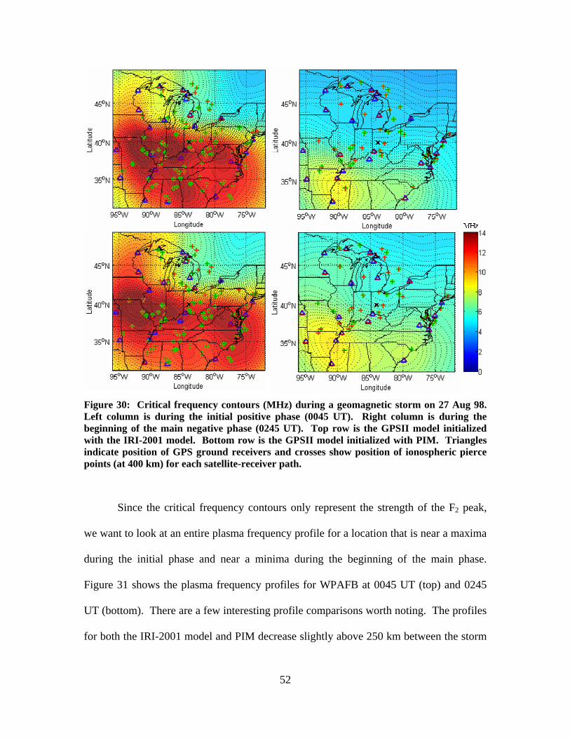
Figure 30: Critical frequency contours (MHz) during a geomagnetic storm on 27 Aug 98. Left column is during the initial positive phase (0045 UT). Right column is during the beginning of the main negative phase (0245 UT). Top row is the GPSII model initialized with the IRI-2001 model. Bottom row is the GPSII model initialized with PIM. Triangles indicate position of GPS ground receivers and crosses show position of ionospheric pierce points (at 400 km) for each satellite-receiver path.

Since the critical frequency contours only represent the strength of the F2 peak,

we want to look at an entire plasma frequency profile for a location that is near a maxima

during the initial phase and near a minima during the beginning of the main phase.

Figure 31 shows the plasma frequency profiles for WPAFB at 0045 UT (top) and 0245

UT (bottom). There are a few interesting profile comparisons worth noting. The profiles

for both the IRI-2001 model and PIM decrease slightly above 250 km between the storm

52

phases, which is expected. The GPSII model has to make significant adjustments in

plasma frequency above 250 km for the initial phase, yet makes much smaller

adjustments for the main phase. PIM’s lower F1 region and upper E region (from 125 km

to 200 km) strengthens slightly between the storm phases. Overall, the plasma

frequencies below 225 km decrease between storm phases for each of the models. What

is most interesting is that the GPSII model, as in case studies #2 and #4, does not make

any adjustments to the E layer, regardless of what is used for its initialization. The TEC

data once more does not aid in specifying the E layer. As we know from our previous

analysis in Case Study #2, we cannot expect TEC measurements to provide much

additional E region information.

53

Figure 31: Plasma frequency (MHz) as a function of height (km) at the approximate apogee of a signal transmitted from Wright-Patterson AFB, OH toward Norfolk, VA for both the initial positive phase (0045 UT, top) and main negative phase (0245 UT, bottom) of a geomagnetic storm on 27 Aug 98 using various ionospheric models.

54

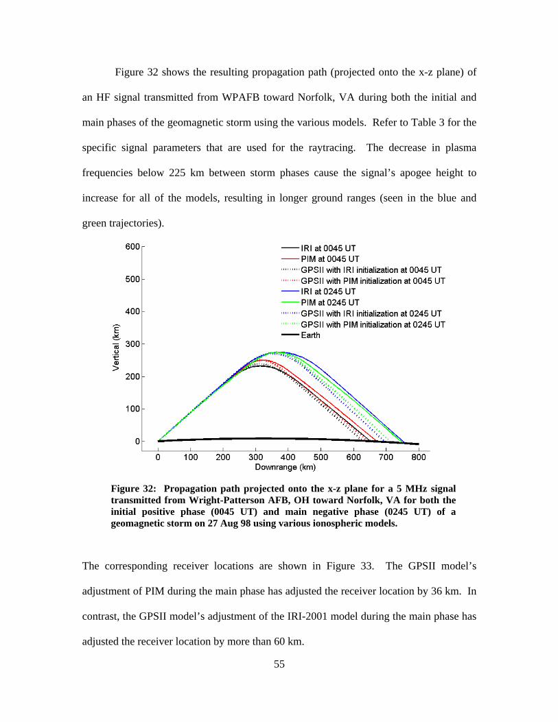
Figure 32 shows the resulting propagation path (projected onto the x-z plane) of

an HF signal transmitted from WPAFB toward Norfolk, VA during both the initial and

main phases of the geomagnetic storm using the various models. Refer to Table 3 for the

specific signal parameters that are used for the raytracing. The decrease in plasma

frequencies below 225 km between storm phases cause the signal’s apogee height to

increase for all of the models, resulting in longer ground ranges (seen in the blue and

green trajectories).

Figure 32: Propagation path projected onto the x-z plane for a 5 MHz signal transmitted from Wright-Patterson AFB, OH toward Norfolk, VA for both the initial positive phase (0045 UT) and main negative phase (0245 UT) of a geomagnetic storm on 27 Aug 98 using various ionospheric models.

The corresponding receiver locations are shown in Figure 33. The GPSII model’s

adjustment of PIM during the main phase has adjusted the receiver location by 36 km. In

contrast, the GPSII model’s adjustment of the IRI-2001 model during the main phase has

adjusted the receiver location by more than 60 km.

55

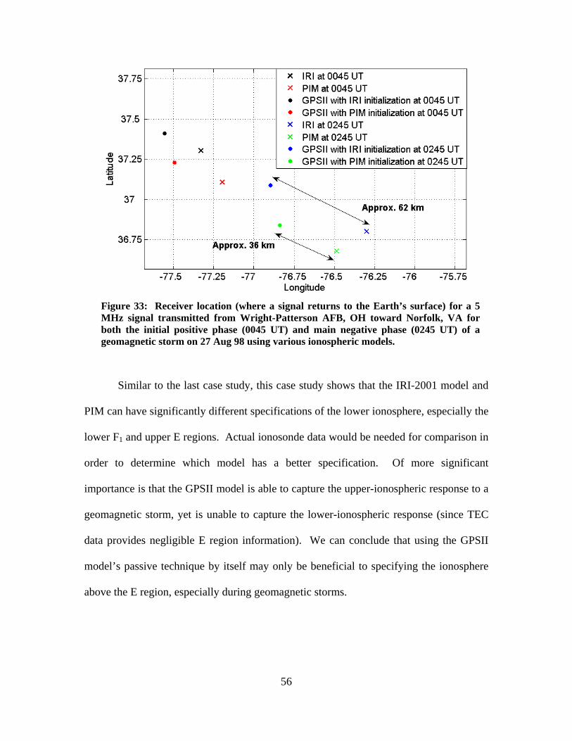
Figure 33: Receiver location (where a signal returns to the Earth’s surface) for a 5 MHz signal transmitted from Wright-Patterson AFB, OH toward Norfolk, VA for both the initial positive phase (0045 UT) and main negative phase (0245 UT) of a geomagnetic storm on 27 Aug 98 using various ionospheric models.

Similar to the last case study, this case study shows that the IRI-2001 model and

PIM can have significantly different specifications of the lower ionosphere, especially the

lower F1 and upper E regions. Actual ionosonde data would be needed for comparison in

order to determine which model has a better specification. Of more significant

importance is that the GPSII model is able to capture the upper-ionospheric response to a

geomagnetic storm, yet is unable to capture the lower-ionospheric response (since TEC

data provides negligible E region information). We can conclude that using the GPSII

model’s passive technique by itself may only be beneficial to specifying the ionosphere

above the E region, especially during geomagnetic storms.

56

Conclusion

Summary

The critical national defense mission of geo-location remains highly dependent on

our ability to accurately measure and predict the dynamic state of the ionosphere. The

primary objective of this thesis was to assess how the IRI-2001, PIM, and GPSII

ionospheric models impact HF signal raytracing during various ionospheric conditions.

The secondary objective was to ascertain whether using passive techniques to model the

ionosphere provide sufficient accuracy for geo-location. Three software components

were used for data collection, processing, and visualization. These included the

ionospheric model, the Hausman – Nickisch update of the Jones – Stephenson raytracing

algorithm, and MATLAB®. Five case studies were used to explore a wide range of

ionospheric conditions; including quiet, daily variability, solar flare, and geomagnetic

storming.

Case study #1 showed how much the E layer by itself could significantly affect a

signal’s ground range and in turn impact the geo-location mission, highlighting the

importance of accurately specifying the lower ionosphere. Case study #2 established a

“base reference” by comparing the models at local noon on a day with quiet solar and

geomagnetic conditions. It showed that the GPSII model was able to adjust for an

unphysical initialization by using TEC data and, as far as quiet conditions were

concerned, it showed that the GPSII model made the smallest adjustments in plasma

frequency when initialized with PIM. More importantly, it provided the first evidence

that the GPSII model may not be able to assist in specifying the E layer. From analyzing

the definition of TEC we were able to determine that the E region’s contribution to

57

vertical TEC is more or less insignificant. Consequently, it is extremely difficult to

extract any reasonable E region information from TEC data alone.

The three remaining case studies focused on isolating certain ionospheric drivers.

Case study #3 examined the daily variability of the ionosphere at local noon over seven

consecutive days of very low solar and geomagnetic activity. The results showed that the

GPSII model may be able to capture the expected daily variability of the ionosphere by

using TEC data. Furthermore, we were able to see how this daily variability had a

considerable affect on the resulting receiver location, which would be even more

pronounced during a period of high solar and geomagnetic activity. Case studies #4 and

#5 were designed to isolate the ionosphere’s response to exclusively a solar flare and a

geomagnetic storm. Case study #4 investigated a strong X3 solar flare that occurred on

15 July 2002 during low geomagnetic activity. Case study #5 explored an intense

geomagnetic storm that occurred on 27 August 1998, in which there were no significant

solar flares throughout its duration. Both case studies showed that the IRI-2001 model

and PIM could have significantly different specifications of the lower ionosphere,

especially the F1 and upper E regions. Actual ionosonde data would be needed for

comparison in order to determine which model had a better specification.

More significantly, the results showed that the GPSII model was able to capture

the upper-ionospheric response to both the solar flare and the geomagnetic storm.

Moreover, they provided further evidence that the GPSII model was not able to capture

the lower-ionospheric response to these events. The TEC data simply did not assist in

specifying the E layer. This suggests that using the GPSII model’s passive technique by

itself may only be beneficial to specifying the ionosphere above the E region, especially

58

during solar flares and geomagnetic storms. We will most likely have to rely on using

active measuring techniques, such as vertical ionosondes, to accurately specify the lower

ionosphere. Fortunately, the GPSII model is designed to incorporate ionosonde data. We

recommend using data from ionosondes that are only located within friendly territory, so

as to maintain as much passivity as possible behind enemy lines.

Future Research

The results from this thesis have generated several ideas for future research:

1) Eliminate the “bulls-eye” pattern (boundary effect) described in case study #2. This

could be accomplished by increasing the latitudinal and longitudinal extent of the GPSII

model’s output. Note that this larger data set would require longer computational time.

MATLAB® could then be used to crop the output data to a smaller region of interest,

thus removing the boundary effect. Of course, the user would have to find a balance

between their computational resources and the mission-dictated region of interest.

2) Determine if there are any model sensitivities when dealing with the lateral refraction

of a signal, otherwise known as the signal’s crossrange. In particular, examine why the

crossrange of a signal can be dependent on the initialization model used. For comparison

in future research, the crossrange plots not included in Chapter IV have been provided in

Appendix D.

3) During the course of our research we were able to identify that a solar radio burst

(concurrent with the solar flare on 15 Jul 02) caused nearly all of the GPS ground

receivers in our region of interest to experience a “loss of lock” of the precision

information embedded within the GPS signal. This radio burst had a peak flux of 1100

solar flux units at 1415 MHz (directly between the L1 and L2 frequency bands of the

59

GPS signal). This precision information, although still encrypted, is used by the civilian

sector to improve GPS accuracy through a technique called “semicodeless tracking”.

This technique will be used until the next-generation GPS constellation is completed in

2012. There is a strong correlation between solar radio bursts and the loss of lock by

semicodeless receivers, as reported by Chen et al. [2005]. Future research could include

exploring the sensitivity of commercial GPS receivers to solar radio bursts that were

previously considered too weak to have any effect. The MATLAB® script created for

this thesis could be used to identify the number of GPS receivers affected by allegedly

weak radio bursts.

4) The newest version of the GPSII model (as of 25 Jan 07) is designed to incorporate

TEC data from low-Earth-orbiting (LEO) satellites. Future research could compare the

GPSII model’s performance when using LEO TEC data versus GPS TEC data.

5) Include ionosonde data as an input for the GPSII model. Compare its specification to

those found in this thesis. Explore how changing the location of the ionosonde affects the

raytracing and geo-location.

6) Finally, use ground truth data to validate the performance of the models when used for

geo-location. Ground truth data would include the measured elevation and azimuth

angles of frequencies received from known radio towers (beacons) as a function of time

during various ionospheric conditions.

Any of these ideas, taken individually or in combination, would be suitable for

future graduate research and could be completed using the same components and

methodology used in this thesis. Continued research in this area will advance our ability

to exploit the ionosphere and mitigate its impact on critical national defense missions.

60

Appendix A: Magnetoionic Splitting

The following figures were created with the raytracing algorithm. Its parameters

were selected in such a way as to produce general magnetoionic splitting behavior.

Figure 34: Magnetoionic splitting of a 10 MHz signal transmitted with elevation = 49o from Wright-Patterson AFB at local noon on the autumnal equinox during normal solar and geomagnetic activity. Shown is crossrange (km) as a function of distance downrange (km) for two transmission azimuths (top = 225o, bottom = 315o; both are not in the direction of one of the four magnetic cardinal points). The signal’s ordinary mode deviates toward magnetic north, while its extraordinary mode deviates toward magnetic south. Signals return to Earth in a plane parallel to the transmission plane but not necessarily coincident with it.

61

Figure 35: Final crossrange (at the point where the signal returns to Earth, in km) as a function of azimuth angle (deg) for HF signals of various frequencies and elevation angles transmitted from Wright-Patterson AFB at local noon on the autumnal equinox during normal solar and geomagnetic activity. Both the ordinary mode (top) and extraordinary mode (bottom) have zero final crossrange near the four magnetic cardinal points. Final crossrange of ordinary mode is opposite in direction to that of the extraordinary mode for all transmission azimuths.

62

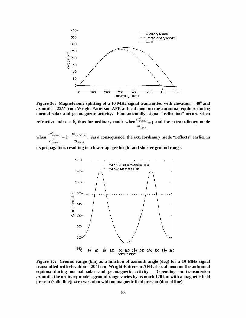
Figure 36: Magnetoionic splitting of a 10 MHz signal transmitted with elevation = 49o and azimuth = 225o from Wright-Patterson AFB at local noon on the autumnal equinox during normal solar and geomagnetic activity. Fundamentally, signal “reflection” occurs when

refractive index = 0, thus for ordinary mode when2

2 1plasma

signal

ωω

= and for extraordinary mode

when 2

2 1plasma cyclotron

signal signal

ω ωω ω

= − . As a consequence, the extraordinary mode “reflects” earlier in

its propagation, resulting in a lower apogee height and shorter ground range.

Figure 37: Ground range (km) as a function of azimuth angle (deg) for a 10 MHz signal transmitted with elevation = 20o from Wright-Patterson AFB at local noon on the autumnal equinox during normal solar and geomagnetic activity. Depending on transmission azimuth, the ordinary mode’s ground range varies by as much 120 km with a magnetic field present (solid line); zero variation with no magnetic field present (dotted line).

63

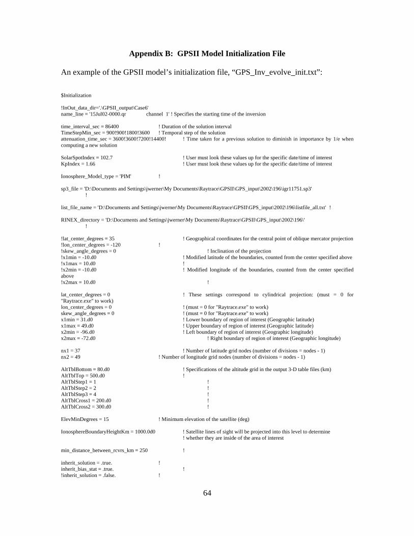
Appendix B: GPSII Model Initialization File

An example of the GPSII model’s initialization file, “GPS_Inv_evolve_init.txt”:

$Initialization !InOut_data_dir='.\GPSII_output\Case6' name_line = '15Jul02-0000.qr channel 1' ! Specifies the starting time of the inversion time_interval_sec = 86400 ! Duration of the solution interval TimeStepMin_sec = 900!900!1800!3600 ! Temporal step of the solution attenuation_time_sec = 3600!3600!7200!14400! ! Time taken for a previous solution to diminish in importance by 1/e when computing a new solution SolarSpotIndex = 102.7 ! User must look these values up for the specific date/time of interest KpIndex = 1.66 ! User must look these values up for the specific date/time of interest Ionosphere_Model_type = 'PIM' ! sp3_file = 'D:\Documents and Settings\jwerner\My Documents\Raytrace\GPSII\GPS_input\2002\196\igr11751.sp3' ! list_file_name = 'D:\Documents and Settings\jwerner\My Documents\Raytrace\GPSII\GPS_input\2002\196\listfile_all.txt' ! RINEX_directory = 'D:\Documents and Settings\jwerner\My Documents\Raytrace\GPSII\GPS_input\2002\196\' ! !lat_center_degrees = 35 ! Geographical coordinates for the central point of oblique mercator projection !lon_center_degrees = -120 ! !skew_angle_degrees = 0 ! Inclination of the projection !x1min = -10.d0 ! Modified latitude of the boundaries, counted from the center specified above !x1max = 10.d0 ! !x2min = -10.d0 ! Modified longitude of the boundaries, counted from the center specified above !x2max = 10.d0 ! lat_center_degrees = 0 ! These settings correspond to cylindrical projection: (must = 0 for "Raytrace.exe" to work) lon_center_degrees = 0 ! (must = 0 for "Raytrace.exe" to work) skew_angle_degrees = 0 ! (must = 0 for "Raytrace.exe" to work) x1min = 31.d0 ! Lower boundary of region of interest (Geographic latitude) x1max = 49.d0 ! Upper boundary of region of interest (Geographic latitude) x2min = -96.d0 ! Left boundary of region of interest (Geographic longitude) x2max = -72.d0 ! Right boundary of region of interest (Geographic longitude) nx1 = 37 ! Number of latitude grid nodes (number of divisions = nodes - 1) nx2 = 49 ! Number of longitude grid nodes (number of divisions = nodes - 1) AltTblBottom = 80.d0 ! Specifications of the altitude grid in the output 3-D table files (km) AltTblTop = 500.d0 ! AltTblStep1 = 1 ! AltTblStep2 = 2 ! AltTblStep3 = 4 ! AltTblCross1 = 200.d0 ! AltTblCross2 = 300.d0 ! ElevMinDegrees = 15 ! Minimum elevation of the satellite (deg) IonosphereBoundaryHeightKm = 1000.0d0 ! Satellite lines of sight will be projected into this level to determine ! whether they are inside of the area of interest min_distance_between_rcvrs_km = 250 ! inherit_solution = .true. ! inherit_bias_stat = .true. ! !inherit_solution = .false. !

64

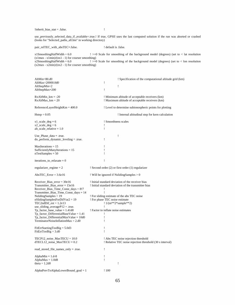
!inherit_bias_stat = .false. ! use_previously_selected_data_if_available=.true.! If true, GPSII uses the last computed solution if the run was aborted or crashed (looks for "Selected_paths_all.bin" in working directory) pair_relTEC_with_absTEC=.false. ! default is .false. x1SmoothingHalfWidth = 6.0 ! >=0 Scale for smoothing of the background model (degrees) (set to < lat resolution (x1max - x1min)/(nx1 - 1) for courser smoothing) x2SmoothingHalfWidth = 6.0 ! >=0 Scale for smoothing of the background model (degrees) (set to < lon resolution (x2max - x2min)/(nx2 - 1) for courser smoothing) AltMin=80.d0 ! Specification of the computational altitude grid (km) AltMax=20000.0d0 ! AltStepMin=2 ! AltStepMax=200 ! RxAltMin_km = -20 ! Minimum altitude of acceptable receivers (km) RxAltMax_km = 20 ! Maximum altitude of acceptable receivers (km) ReferenceLayerHeightKm = 400.0 ! Level to determine subionospheric points for plotting Hstep = 0.05 ! Internal altitudinal step for kern calculation x1_scale_deg = 6 ! Smoothness scales x2_scale_deg = 6 ! alt_scale_relative = 1.0 ! Use_Phase_data = .true. ! do_perform_dynamic_leveling = .true. ! MaxIterations = 15 ! SufficientlyManyIterations = 15 ! nTestSamples = 50 ! iterations_to_relaxate = 0 ! regularizer_regime = 2 ! Second order (2) or first order (1) regularizer AbsTEC_Error = 3.6e16 ! Will be ignored if NslidingSamples > 0 Receiver_Bias_error = 30e16 ! Initial standard deviation of the receiver bias Transmitter_Bias_error = 15e16 ! Initial standard deviation of the transmitter bias Receiver_Bias_Time_Const_days = 8!7 ! Transmitter_Bias_Time_Const_days = 14 ! NslidingSamples = 19 ! For sliding estimate of the abs TEC noise nSlidingSamplesForDifVar2 = 19 ! For phase TEC noise estimate TEC2ndDif_est = 1.2e13 ! 1/(m**2*sample**2) use_sliding_averageP12 = .true. ! Tp_factor_base_value = 1.41d0 ! Factor to inflate noise estimates Tp_factor_DifferentialBaseValue = 1.41 ! Tp_factor_DifferentialMaxValue = 10d0 ! TerminatorNoiseInflationMax = 2.d0 ! FitErrStartingTooBig = 5.0d3 ! FitErrTooBig = 3.d0 ! TECP12_noise_MaxTECU = 10.0 ! Abs TEC noise rejection threshold dTECL12_noise_MaxTECU = 0.2 ! Relative TEC noise rejection threshold (30 s interval) read_stored_file_names_only = .true. ! AlphaMin = 1.d-8 ! AlphaMax = 1.0d8 ! theta = 1.2d0 ! AlphaPrevToAlphaLowerBound_goal = 1 ! 100

65

AlphaPrevToAlphaUpperBound_goal = 1000.0 ! Finish it AlphaPrevEnforcementStartTStep = -10000 ! WriteTECforPlotting = .true. ! dTEC_threshold_TECU = 1.d0 ! Rejection threshold for testing of the first difference ! of the phase-based TEC series per RINEX sampling period (usu 30s) dTEC_rate_threshold_TECU = 0.1d0 ! Rejection threshold for testing second difference ! of the phase-based TEC series per RINEX sampling period (usu 30s) AttenuationFactorForTderivative = 0.0d0 ! A value from 0.0 to 1.0. ! Zero corresponds to using zero order extrapolation from the previous ! time step for starting solution on the current step ! One corresponds to linear extrapolation OptimizeAttenuation = .true. ! <=> Select the best starting solution among solutions obtained ! with zero order extrapolation and with AttenuationFactorForTderivative CenterAltitudeWithLowVariabilityKm = 285.d0 ! AltScaleLowVarability = 150.0d0 ! RelMagnitudeOfHighVariability = 1.d0 ! diagonalProfCov = .true. ! .false. $end ******************************************************************* *************************QVI Sounders information****************** -------------------------------------------------------------------------------------- SounderID,SounderLat,SounderLon(degrees decimal),nefitFileName,ProfileFileName,ref_prof_spec,match_fof2_spec,[DeltaProfFpRel,DeltaProfFpMHz,DeltaProfHkm,[Abovekm]] -------------------------------------------------------------------------------------- *************************End QVI Sounders************************** ******************************************************************* 'ARGUELLO' 35.6, -120.6 'nefit1.par' '06Sep04-1500-PA836_profile.tbl' 'table' 'match fof2' 'BOULDER' 40.0, -105.3 'nefit1.par' '07Aug06-1530-BC840_profile.tbl' 'table' 'match fof2' 0.03 0.10 20.0 0.0 !'VA_ROTHR' 36.4684, -76.2592 'nefit_v.par' '_qviscale_v.tbl' 'table' 'match fof2' !Project directories: !http://gaim.cass.usu.edu/JULY2001/GAIMHTML/page34.html !http://www.aiub.unibe.ch/download/CODE/CODE.ACN !http://www.ngs.noaa.gov/GPS/GPS.html !http://140.96.176.15/GPS_WEEK/calendar.y97

66

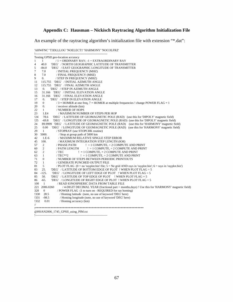
Appendix C: Hausman – Nickisch Raytracing Algorithm Initialization File

An example of the raytracing algorithm’s initialization file with extension “*.dat”:

'AHWFNC' 'T3DLLLOG' 'NOELECT1' 'HARMONY' 'NOCOLFRZ' !----------------------------------------------------------------------- Testing GPSII geo-location accuracy 1 1 / 1 = ORDINARY RAY; -1 = EXTRAORDINARY RAY 4 40.0 'DEG' / NORTH GEOGRAPHIC LATITUDE OF TRANSMITTER 5 -84.0 'DEG' / EAST GEOGRAPHIC LONGITUDE OF TRANSMITTER 7 7.0 / INITIAL FREQUENCY (MHZ) 8 7.0 / FINAL FREQUENCY (MHZ) 9 0. / STEP IN FREQUENCY (MHZ) 11 115.755 'DEG' / INITIAL AZIMUTH ANGLE 12 115.755 'DEG' / FINAL AZIMUTH ANGLE 13 0. 'DEG' / STEP IN AZIMUTH ANGLE 15 31.166 'DEG' / INITIAL ELEVATION ANGLE 16 31.166 'DEG' / FINAL ELEVATION ANGLE 17 0. 'DEG' / STEP IN ELEVATION ANGLE 19 0 / 3 = HOMER at one freq, 7 = HOMER at multiple frequencies ! change POWER FLAG = 1 20 0. / receiver altitude (km) 22 1 / NUMBER OF HOPS 23 1.E4 / MAXIMUM NUMBER OF STEPS PER HOP !24 78.6 'DEG' / LATITUDE OF GEOMAGNETIC POLE (RAD) (use this for 'DIPOLY' magnetic field) !25 -69.8 'DEG' / LONGITUDE OF GEOMAGNETIC POLE (RAD) (use this for 'DIPOLY' magnetic field) 24 89.9999 'DEG' / LATITUDE OF GEOMAGNETIC POLE (RAD) (use this for 'HARMONY' magnetic field) 25 0.00 'DEG' / LONGITUDE OF GEOMAGNETIC POLE (RAD) (use this for 'HARMONY' magnetic field) 29 1 / STOPRAY (use STOPCHK routine) 30 5000. / Stop at group path of 5000 km 42 1.E-6 / MAXIMUM RELATIVE SINGLE STEP ERROR 45 100. / MAXIMUM INTEGRATION STEP LENGTH (KM) 57 2 / PHASE PATH ! = 1 COMPUTE, = 2 COMPUTE AND PRINT 60 2 / PATH LENGTH ! = 1 COMPUTE, = 2 COMPUTE AND PRINT 62 2 / TEC ! = 1 COMPUTE, = 2 COMPUTE AND PRINT 63 1 / TEC**2 ! = 1 COMPUTE, = 2 COMPUTE AND PRINT 71 0 / NUMBER OF STEPS BETWEEN PERIODIC PRINTOUTS 72 1 / GENERATE PUNCHED OUTPUT FILE 81 5 / PLOT FLAG (0 = no 'rayplot.bin' file; 5 = Ne grid AND rays in 'rayplot.bin'; 6 = rays in 'rayplot.bin') 83 25. 'DEG' / LATITUDE OF BOTTOM EDGE OF PLOT ! WHEN PLOT FLAG = 5 84 -125. 'DEG' / LONGITUDE OF LEFT EDGE OF PLOT ! WHEN PLOT FLAG = 5 85 50. 'DEG' / LATITUDE OF TOP EDGE OF PLOT ! WHEN PLOT FLAG = 5 86 -65. 'DEG' / LONGITUDE OF RIGHT EDGE OF PLOT ! WHEN PLOT FLAG = 5 100 1 / READ IONOSPHERIC DATA FROM TABLE FILE 221 2006.0260 / 4-DIGIT DECIMAL YEAR (fractional part = months,days) ! Use this for 'HARMONY' magnetic field) 320 0 / POWER FLAG (1 to turn on - REQUIRED for ray homing) !330 28.5 / Homing latitude (note, no use of keyword 'DEG' here) !331 -98.5 / Homing longitude (note, no use of keyword 'DEG' here) !332 0.01 / Homing accuracy (km) // !*********************************************************************** @09JAN2006_1745_GPSII_using_PIM.txt !-----------------------------------------------------------------------

67

Appendix D: Crossrange Plots

Figure 38: Crossrange (km) as a function of distance downrange (km) for a 6 MHz and 8 MHz signal transmitted with elevation = 35o and azimuth = 180o from Wright-Patterson AFB, OH at local noon on the autumnal equinox during normal solar and geomagnetic activity. Two ionospheres are used; one has an E layer (solid lines), the other does not have an E layer (dotted lines).

Figure 39: Crossrange (km) as a function of distance downrange (km) for a 7 MHz signal transmitted with elevation = 31.166o from Wright-Patterson AFB, OH toward Norfolk, VA at local noon on 9 Jan 06 (quiet solar and geomagnetic conditions) using various ionospheric models.

68

Figure 40: Crossrange (km) as a function of distance downrange (km) for an 8 MHz signal transmitted with elevation = 40.260o from Wright-Patterson AFB, OH toward Norfolk, VA both before (2000 UT) and during (2015 UT) a solar flare on 15 Jul 02 using various ionospheric models.

Figure 41: Crossrange (km) as a function of distance downrange (km) for a 5 MHz signal transmitted with elevation = 38.657o from Wright-Patterson AFB, OH toward Norfolk, VA during the initial positive phase (0045 UT) and the beginning of the main negative phase (0245 UT) of a geomagnetic storm on 27 Aug 98 using various ionospheric models.

69

Bibliography

Aune, S. C. (2006), Comparison of ray tracing through ionospheric models, M.S. thesis, Air Force Institute of Technology, Wright-Patterson Air Force Base, Ohio.

Bilitza, D. (2001), International Reference Ionosphere 2000, Radio Science, 36(2), 261-275.

Budden, K. G. (1985), The propagation of radio waves: the theory of radio waves of low power in the ionosphere and magnetosphere, Cambridge University Press, Cambridge, New York.

Chen, Z., Y. Gao, and Z. Liu (2005), Evaluation of solar radio bursts’ effect on GPS receiver signal tracking within International GPS Service network, Radio Science, 40, RS3012, doi:10.1029/2004RS003066.

Coleman, C. J. (1998), Ray tracing formulation and its application to some problems in over-the-horizon radar, Radio Science, 33(4), 1187-1197.

Daniell, R. E., L. D. Brown, D. N. Anderson, M. W. Fox, P. H. Doherty, D. T. Decker, J. J. Sojka, and R. W. Schunk (1995), Parameterized ionospheric model: A global ionospheric parameterization based on first principles models, Radio Science, 30(5), 1499-1510.

Davies, K. (1989), Ionospheric radio, Peter Peregrinus Ltd., London, U.K.

Doherty, B. D. (2004), A statistical analysis of ionospheric echoes detected by the TIGER SuperDARN radar, B.S. thesis, La Trobe University, Bundoora, Victoria

Fridman, S. V., L. J. Nickisch, M. Aiello, and M. Hausman (2006), Real-time reconstruction of the three-dimensional ionosphere using data from a network of GPS receivers, Radio Science, 41, RS5S12, doi:10.1029/2005RS003341.

Hamilton, W. R., Sir (1832), Third supplement to an essay on the theory of systems of rays, Trans. Royal Irish Acad., 17(144), 1-144.

Hargreaves, J.K. (1992), The solar-terrestrial environment, Cambridge University Press, Cambridge, New York.

Haselgrove, J. (1954), Ray theory and a new method for ray tracing, Report of Conference on the Physics of the Ionosphere, London Physical Society, London, U.K.

70

Haselgrove, C. B., and J. Haselgrove (1960), Twisted ray paths in the ionosphere, Proc. Phys. Soc. London, 75(5), 357-361.

Huang, X., and B. W. Reinisch (2006), Real-time HF ray tracing through a tilted ionosphere, Radio Science, 41(8).

Jones, R. M., and J. J. Stephenson (1975), A versatile three-dimensional ray tracing computer program for radio waves in the ionosphere, Institute for Telecommunication Sciences, U.S. Dept. of Commerce, Office of Telecommunications, Washington.

Kelso, J. M. (1964), Radio ray propagation in the ionosphere, McGraw-Hill, New York.

McDonnell, M. D. (2000), A fast three-dimensional ray tracing formulation, with applications to HF communications and RADAR predictions, report, Dept. of Electrical and Electronic Engineering, The University of Adelaide, South Australia.

McNamara, L. F. (1991), The ionosphere: communications, surveillance, and direction finding, Krieger Publishing Company, Malabar, Florida.

Nickisch, L. J. (1988), Focusing in the stationary phase approximation, Radio Science, 23(2), 171-182.

Schunk, R. W., and A. Nagy (2000), Ionospheres: physics, plasma physics, and chemistry, Cambridge University Press, Cambridge, New York.

Strangeways, H. J. (1997), HF transmitter location using super-resolution DF and ionospheric sounding, AGARD SPP Symposium on “Multi-Sensor Systems and Data Fusion for Telecommunication, Remote Sensing and Radar”, NATO, Lisbon, Portugal.

Sturrock, P. A. (1994), Plasma physics: an introduction to the theory of astrophysical, geophysical, and laboratory plasmas, Cambridge University Press, Cambridge, New York.

71

Form Approved REPORT DOCUMENTATION PAGE OMB No. 074-0188

The public reporting burden for this collection of information is estimated to average 1 hour per response, including the time for reviewing instructions, searching existing data sources, gathering and maintaining the data needed, and completing and reviewing the collection of information. Send comments regarding this burden estimate or any other aspect of the collection of information, including suggestions for reducing this burden to Department of Defense, Washington Headquarters Services, Directorate for Information Operations and Reports (0704-0188), 1215 Jefferson Davis Highway, Suite 1204, Arlington, VA 22202-4302. Respondents should be aware that notwithstanding any other provision of law, no person shall be subject to an penalty for failing to comply with a collection of information if it does not display a currently valid OMB control number. PLEASE DO NOT RETURN YOUR FORM TO THE ABOVE ADDRESS. 1. REPORT DATE (DD-MM-YYYY) 2. REPORT TYPE 3. DATES COVERED (From – To)

Master’s Thesis 22-03-2007 Aug 2006 – Mar 2007 5a. CONTRACT NUMBER 4. TITLE AND SUBTITLE

5b. GRANT NUMBER

Assessment of the Impact of Various Ionospheric Models on High-Frequency Signal Raytracing 5c. PROGRAM ELEMENT NUMBER

5d. PROJECT NUMBER 5e. TASK NUMBER

6. AUTHOR(S) Werner, Joshua T., 1Lt, USAF 5f. WORK UNIT NUMBER

7. PERFORMING ORGANIZATION NAMES(S) AND ADDRESS(S) Air Force Institute of Technology Graduate School of Engineering and Management (AFIT/EN) 2950 Hobson Way, Building 640 WPAFB OH 45433-7765

8. PERFORMING ORGANIZATION REPORT NUMBER AFIT/GAP/ENP/07-07

10. SPONSOR/MONITOR’S ACRONYM(S)

9. SPONSORING/MONITORING AGENCY NAME(S) AND ADDRESS(ES)

11. SPONSOR/MONITOR’S REPORT NUMBER(S)

12. DISTRIBUTION/AVAILABILITY STATEMENT APPROVED FOR PUBLIC RELEASE; DISTRIBUTION UNLIMITED

13. SUPPLEMENTARY NOTES 14. ABSTRACT An assessment of the impact of various ionospheric models on high-frequency (HF) signal raytracing is presented. Ionospheric refraction can strongly affect the propagation of HF signals. Consequently, Department of Defense missions such as over-the-horizon RADAR, HF communications, and geo-location all depend on an accurate specification of the ionosphere. Five case studies explore ionospheric conditions ranging from quiet conditions to solar flares and geomagnetic storms. It is shown that an E layer by itself can increase an HF signal’s ground range by over 100 km, stressing the importance of accurately specifying the lower ionosphere. It is also shown that the GPSII model has the potential to capture the expected daily variability of the ionosphere by using Total Electron Content data. This daily variability can change an HF signal’s ground range by as much as 5 km per day. The upper-ionospheric response to both a solar flare and a geomagnetic storm is captured by the GPSII model. In contrast, the GPSII model does not capture the lower-ionospheric response to either event. These results suggest that using the GPSII model’s passive technique by itself may only be beneficial to specifying the ionosphere above the E region, especially during solar flares and geomagnetic storms. 15. SUBJECT TERMS Ionosphere, electromagnetic wave propagation, ionospheric propagation, radio transmission, ray tracing, ionospheric model, global positioning system, solar disturbances, solar flares, magnetic storms 16. SECURITY CLASSIFICATION OF:

19a. NAME OF RESPONSIBLE PERSON Christopher G. Smithtro, Maj, USAF (ENP)

18. NUMBER

17. LIMITATION OF

OF ABSTRACT 19b. TELEPHONE NUMBER (Include area code) a. REPORT

U

b. ABSTRACT

U

c. THIS PAGE

PAGES (937) 255-3636, ext 4505

christopher.smithtro@afit.edu U 84 UU Standard Form 298 (Rev. 8-98)

Prescribed by ANSI Std. Z39-18