aerodynamic heating simulation. part 1. theory and program definition

A~~ ~~ '(1(P 507

FDL TDR 64-112PART I

0) AERODYNAMIC HEATING SIMULATION(00O PART I. THEORY AND PROGRAM DEFINITION0)

0 GLENDON R. CRUMP, LT, USAF

00SJ TECHNICAL DOCUMENTARY REPORT No. FDL TDR 64-112, PART I

SEPTEMBER 1964

AF FLIGHT DYNAMICS LABORATORYRESEARCH AND TECHNOLOGY DIVISION

AIR FORCE SYSTEMS COMMANDWRIGHT-PATTERSON AIR FORCE BASE, OHIO

Project No. 1347, Task No. 134703

Best Available Copy

NOTICES

When Government drawings, specifications, or other data are used forany purpose other than in connection with a definitely related Governmentprocurement operation, the United States Government thereby incurs noresponsibility nor any obligation whatsoever; and the fact that the Govern-ment may have formulated, furnished, or in any way supplied the said draw-ings, specifications, or other data, is not to be regarded by implication orotherwise as in any manner licensing the holder or any other person orcorporation, or conveying any rights or permission to manufacture, use,or sell any patented invention that may in any way be related thereto.

Qualified requesters may obtain copies of this report from the DefenseDocumentation Center (DDC), (formerly ASTIA), Cameron Station, Bldg. 5,5010 Duke Street, Alexandria, Virginia, 22314.

This report has been released to the Office of Technical Services, U.S.Department of Commerce, Washington 25, D. C., in stock quantities forsale to the general public.

Copies of this report should not be returned to the Research and Tech-nology Division, Wright-Patterson Air Force Base, Ohio, unless returnis required by security considerations, contractual obligations, or noticeon a specific document.

200 - Novenber 1964 - 448-11-312

FDL TDR 64-112Part I

FOREWORD

This report was prepared in-house under Project No. 1347, "Structural Testing ofFlight Vehicles," Task No. 134703, "Structural Testing Criteria." The work wasconducted by the Experimental Mechanics Branch, Structures Division, Air Force FlightDynamics Laboratory, with Mr. W. R. Johnston acting as task engineer.

Best Available Copy

FDL TDR 64-112

Part I

ABSTRACT

This study was conducted to determine how accurately aerodynamic heating issimulated in the laboratory with radiant heat lamps under computer control. A studyof aerodynamic heating theory resulted in the preparation of a digital computer programfor calculating the parameters required as input data for the heat rate computer. Theheat rate computer is used to control the heat input to an actual flight test specimen.Laboratory test results are compared with flight measured data to determine the degreeof simulation. Test results indicate that aerodynamic heating may be adequatelysimulated up to 600'F. Laboratory simulation to higher temperatures are being studiedfor future programs.

This technical documentary report has been reviewed and is approved.

HOL ES, JR.Actg Chief, Structures DivisionAF Flight Dynamics Laboratory

iii


TABLE OF CONTENTS

SECTION PAGE

INTRODUCTION I

Aerodynamic Heating 1

THE HEAT BALANCE EQUATION 2

THE TEST PROGRAM 3

CONCLUSIONS 4

REFERENCES 10

APPENDIX I. IBM Digital Computer Program 11

APPENDIX II. Special Purpose Heat Rate Computer 19

iv


SYMBOLS

SYMBOL DEFINITION UNITS

A Area Ft3

B Emissivity factor (,Ea) BTU/hr-ft- -0 R4

B-h B-h SCALE FACTOR potentiometer setting

c Specific heat of the skin material BTU/lb-_R

C Specific heat of air BTU/lb-*RP

Cput C SCALE FACTOR potentiometer setting ---

C switch C SCALE FACTOR switch position

E Voltage Volts

Ae Error signal Volts

E1 gain Inherent gain associated with the EI RANGEswitch position

G Gain ---

G Nocturnal irradiation BTU/hr-ft2

G Solar irradiation BTU/hr-ft2

g Acceleration due to gravity Ft/sec2

h Convective heat transfer coefficient BTU/hr-ft2 -OR

H Adiabatic wall enthalpy BTU/lbaw

H Skin enthalpy BTU/lb

I Current Amperes

J Conversion factor (778) Ft-lb/BTU

KD Demand gain

Kpot K SCALE FACTOR potentiometer setting

V

FDL TDR 64-112

Part I

SYMBOLS (Continued)


P.B. Offset Proportional band offset OR

qe Heat input from equipment BTU/hr-ft2

qloss Total heat losses due to internal BTU/hr-ft2

convection, conduction, and radiation

r Recovery factor ---

T Adiabatic wall temperature ORaw

Tf Local free stream temperature OR

T Effective temperature of space ORr

T Skin temperature ORs

stag Stagnation temperature OR

T Programmed skin temperature ORsp

T st Test skin temperature OR

T T RANGE switch position ORs range s

t Time Hr

V Velocity Ft/sec

w Specific weight of the skin material Lb/ft3

Y Conversion factor BTU/hr-watt

of 0Nocturnal absorbtivity

o Solar absorbtivitys

Skin emissivity

vi


SYMBOLS (Continued)


77 Efficiency

a Stefan-Boltzmann constant (1.73 x 10-9) BTU/hr-ft-°R'

r Skin thickness Ft

vii

FDL TDR 64-112

Part I

COMPUTER PROGRAM SYMBOLS


H Altitude Feet

VA Velocity of the vehicle Ft/sec

THETA Time Sec

TS Skin temperature OR

DTS Derivative of skin temperature with respect °R/secto time, dT/de

XMN Free stream Mach number

T2 Temperature of the air aft of the shock wave OR

RN2 Reynolds number aft of the shock wave ---

TTS Temperature values for table used to find °Rskin emissivity and specific heat

ES Emissivity of the skin material ---

CPS Specific heat of the skin material BTU/lb--R

DTSI Derivative of skin temperature with respect °R/secto the time used in the Runge-Kutta calculations

ALFD Angle of attack Degrees

TAW Adiabatic wall temperature OR

HTC Aerodynamic heat transfer coefficient BTU/hr-ft-•-R

Q Total heat transferred BTU/hr-ft2

TAWP Adiabatic wall temperature scaled for punching ---

on tape for use on the heat rate computer

HP Aerodynamic heat transfer coefficient scaled ---

for punching on tape for use on the heat ratecomputer

TSP Skin temperature scaled for punching on tapefor use on the heat rate computer

K Number of points

viii

FDL TDR 64-112

Part I

COMPUTER PROGRAM SYMBOLS (Continued)


PRP Prandtl Number raised to the -2/3 power

RNCR Critical Reynolds number ---

D7 Wedge angle Degrees

ELH Distance from leading edge to the point in Feetquestion

RHOS Density of the skin material Lbs/ft3

DELTAS Skin thickness Feet

DELTAH Time interval used in Runge-Kutta calculations Sec

ESA Average material emissivity ---

HGP Altitude Meters

Al, A2, A3 Constants for atmospheric calculations

TB Atmospheric temperature constant OR

PB Atmospheric pressure constant Lbs/ft2

RHOB Atmospheric density constant Slugs/ft3

HB Altitude constant Meters

P Local atmospheric pressure Lbs/ft2

RHO Local atmospheric density Slugs/ft3

TM Local molecular-scale temperature of the ORatmosphere

VS Local speed of sound Ft/sec

VIS Local kinematic viscosity of the atmosphere Fe /sec

T Local temperature of the atmosphere OR

A, B, C, D Constants for finding the atmospheric ---

temperature

ALFHD Wedge angle plus angle of attack (D7+ALFD) Degrees

ix

FDL TDR 64-112

Part I



P2 Pressure aft of the shock wave Lbs/ft2

RHO2 Density of the air aft of the shock wave Slugs/ft3

V2 Velocity aft of the shock wave Ft/sec

ALFHR (D7 + ALFD)/57.3 Radians

CP Pressure coefficient

XMNN Mach number normal to the shock wave ---

BETA Shock wave angle Radians

XMN2 Mach number aft of the shock wave ---

BMU2 Coefficient of viscosity aft of the shock wave Lb/ft-sec

CH, YH, RH Constants depending on Reynolds Number (RH is ---

the recovery factor)

Dl, D2, D3 Constants used in calculating enthalpies

H2 Enthalpy aft of the shock wave BTU/lb

HAW Adiabatic wall enthalpy BTU/lb

HS Skin enthalpy BTU/lb

HR Reference enthalpy BTU/lb

D4, D5, D6 Constants used in calculating temperatures ---

TH Temperature based on reference enthalpy OR

BMUH Coefficient of viscosity based on reference enthalpy Lb/ft-sec

RHOH Density based on reference enthalpy Lb/ft3

RNH Reynolds Number based on reference enthalpy ---

SBC Stefan-Boltzmann constant (4.758 x 10-13) BTU/sec-ft3 - *R4

TSA Temperature used in Runge-Kutta calculations OR

x

FDL TDR 64-112

Part I



DTA, DTB, DTC Derivative of temperature with respect to time *R/secused in Runge-Kutta calculations

CPA Specific heat of air BTU/lb-*R

BC Average emissivity multiplied by the Stefan- BTU/sec-ft2 -*R4Boltzmann constant

HMAX Maximum aerodynamic heat transfer coefficient BTU/hr-ft3 -*R

TAWMAX Maximum adiabatic wall temperature OR

BH Calculated setting for the heat rate computer ---

B-h potentiometer

DK Demand gain obtained in scaling for the heat ---

rate computer

TAWR Adiabatic wall temperature range for the heat ORrate computer

TSMAX Maximum skin temperature OR

TSR Skin temperature range for the heat rate ORcomputer

xi

FDL TDR 64-112

Part I

INTRODUCTION

This program was conducted to determine if elevated temperature test techniquesused in the Structures Test Facility of the Air Force Flight Dynamics Laboratoryprovide an acceptable simulation of aerodynamic heating. A background study ofaerodynamic heating theory was performed and a digital computer program waswritten to provide the necessary information for use on a heat control computer.Thermal simulation tests were conducted on a flight test article, and the laboratorytest temperatures were compared with the flight test temperatures to determine thedegree of simulation.

AERODYNAMIC HEATING

When a flight vehicle moves through the earth's atmosphere, the relative motionbetween the vehicle and the air creates a flow boundary layer (Reference 1). Thefrictional forces between the vehicle and the boundary layer convert the energy ofthe moving air into heat. The amount of heat transferred to the vehicle surface isdependent upon the difference between the boundary layer temperature and the skintemperature, and the coefficient of heat transfer. The rate of change of the skintemperature depends on the rate of heat exchange and the heat capacity of the skin

structure. If steady-state aerodynamic conditions are maintained for a sufficient time,a condition will result wherein aerodynamic heat input equals the total heat losses, thusresulting in a constant surface temperature.

Some of the heat generated by the aerodynamic conditions is dissipated, or lost, from

the vehicle's surface by radiation. At low velocities the skin temperatures are low and

the resultant radiation losses are an insignificant portion of the total heat transferred.At large Mach numbers, and therefore high temperatures, the amount of heat radiatedby the surface may be a large percentage of the heat transferred.

The aerodynamic heating properties are based on the local free stream conditions

at the point of the vehicle under consideration. At velocities greater than the speed of

sound, shock and expansion areas are produced that create local conditions different

from the surrounding ambient atmospheric conditions. The changes that take place are

dependent upon the shape of the vehicle. All of the calculations in this study are based on

a wedge-shaped body. Although a large amqunt of the information in this report is

applicable to any shape, many of the calculations in the digital computer programwould require changing for use with any shape other than a wedge.

Manuscript released by author 7 July 1964 for publication as an RTD TechnicalDocumentary Report.

1

FDL TDR 64-112

Part I

THE HEAT BALANCE EQUATION

In order to investigate aerodynamic heating thououghly, all possible heat inputs andlosses must be recognized. For illustrative purposes, consider a flat plate insulatedon all surfaces except the heated surface and subjected to an aerodynamic heatingenvironment. The immediate environmental temperature will depend only on the vehiclealtitude and velocity. The stagnation temperature is expressed by the following equation:

V2

Tso = Tf +ta + 2g JCp

The temperature of the air stream next to the surface (the adiabatic wall temperature)is related to the ambient temperature and the stagnation temperature by the followingexpression:

r V2

Ta= Tf + og JCP

The amount of heat that reaches the surface of the vehicle is dependent upon the valueof the convective heat transfer coefficient. This heat is represented by the expressionh(Taw - T s). Additional heat may be obtained by irradiation from surrounding bodies

such as the earth and the sun. If the vehicle is radiating to space, the surface will loseheat according to the term crTs 4. The heat capacity of the plate per unit time can be

expressed as cw'r -) The previous terms can be combined to form the following thedt

balance equation:

dTs = h (Taw- Ts ) +4 at G1 +as G5 -E0 T4cw T dt R ssT

It must be emphasized that this expression represents the idealized case of a uniformlyheated insulated plate with a unit area, constant thickness, and uniform materialproperties.

Since the idealized case seldom exists in actual flight, the basic heat balance equationmust be modified to include other sources of heat inputs and losses. Additionalheat inputs may be obtained from engines, electronic devices, electric motors, andother heat generating equipment. Heat may be lost by conduction to adjacent structure,internal convection and radiation, and through active cooling equipment. The heatbalance equation can now be written as follows:

d Ts

cwr dT- = h(To -Ts )+ ap Gp + a + q9 - --4 o-dt os losse+.

where q erepresents additional heat inputs, and ql1 s represents additional heat losses.

2

"FDL TDR 64-112Part I

During accelerated or decelerated atmospheric flight some of the terms becomerelatively insignificant. For instance, solar and nocturnal irradiation is significant onlyin space operations. Similarly, the heat generated by equipment is often a very smallpercentage of the heat generated by aerodynamic heating. By eliminating these insignifi-cant factors the heat balance equation may be expressed as follows:

dTs 4

cw" h (Taw--) EoTs lossThis equation is the basis for the closed loop, computer controlled aerodynamic heating

simulation tests.

THE TEST PROGRAM

When conducting elevated temperature tests, the philosophy is to simulate the externalthermal environment and allow the structure to distribute the heat as it would in actualflight. This method is in contrast to the philosophy of adjusting the external testenvironment until some predicted internal temperature distribution is obtained. Inaddition, the specimen is used as a calorimeter, and the surface temperature is fedback from each control area to the computer which calculates any power changerequired. This instrumentation and control feature contrasts to the method in whichheat flux gages were used by some French and British investigators.

It is obvious that radiant heating is different from convective heating and does notduplicate the mass flow encountered by a vehicle moving through the earth's atmosphere.The objectives of this program were to determine the validity of the laboratory's testphilosophy and the accuracy of aerodynamic heating simulation using radiant heatlamps under computer control. If the temperature distribution obtained with radiantheating is the same as that obtained during flight, then it may be assumed that theaerodynamic thermal environment has been adequately simulated. In this study thelaboratory test temperatures were compared with flight measured temperatures todetermine the accuracy of laboratory simulation.

This study is also concerned with the adequacy of the design equations for the GeneralElectric Heat Rate Computer, which is used for control of most elevated temperaturetests conducted in this laboratory. Of particular interest is the computer limitation thatconstants be used for temperature dependent variables. For instance, the specimenemissivity and specific heat are known to vary with temperature, but a constant valuemust be used in setting up the computer (Reference 2). Similarly, the efficiency of atest setup will vary as the temperature and temperature rise rate change, but againthe computer requires that the efficiency be considered a constant. In addition, since thecomputer's design equations were based on an idealized insulated plate, informationwas desired on what effect adjacent heat sources, heat sinks, and various structuralmembers would have on the computer's control characteristics. The effects these factorshave on thermal simulation tests are important for determining design requirements forfuture heat control computers.

3


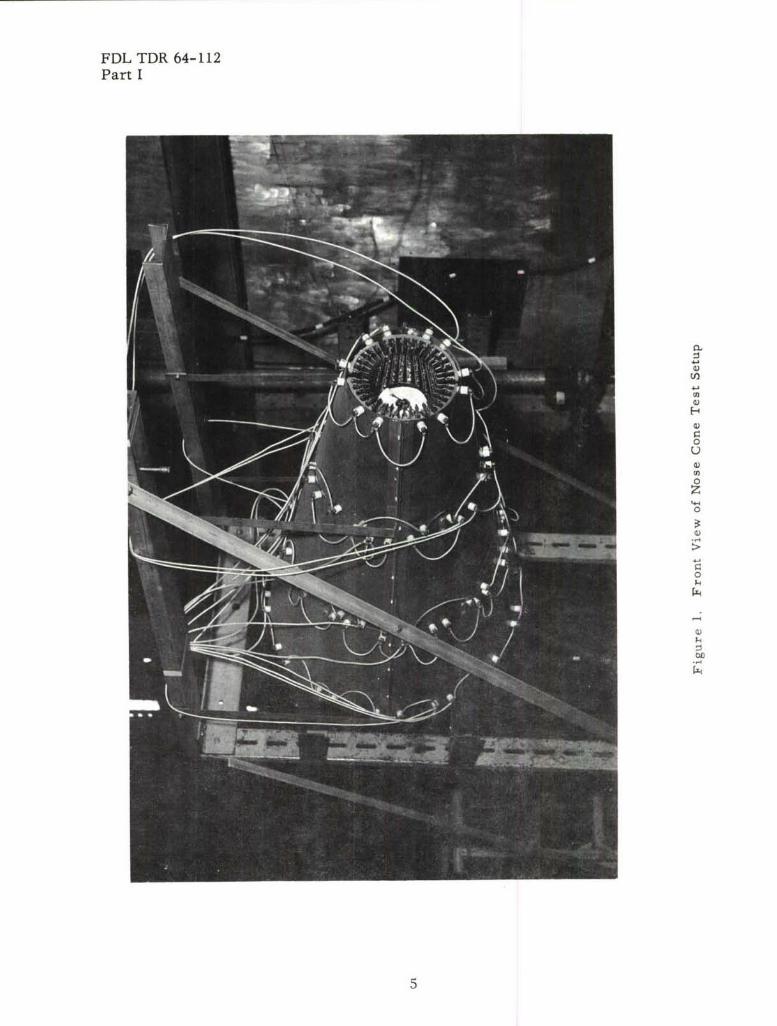
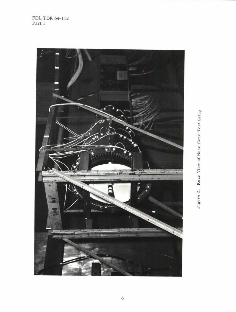
Two test specimens, with complete flight data, were available. A nose cone specimen(a polished stainless steel truncated cone shell) was fabricated to be a duplicate of aViking 10 rocket nose cone. Information for nose cone construction and test correlationwas obtained from NRL Report 4531. "Flight Measurements of Aerodynamic Heating andBoundary-Layer Transition on the Viking 10 Nose Cone" (Reference 3). Care was takenin the laboratory setup, shown in Figures 1 and 2, to duplicate the flight conditions asclosely as possible. Twenty-five thermocouples were installed on the specimen,nineteen internal data thermocouples and six external control thermocouples. The nosecone was divided into three thermal control areas, with maximum temperatures ofapproximately 300'F. Because of low temperatures and resultant low power require-ments, the nose cone was abandoned in favor of the X-7A wedge-shaped wing.

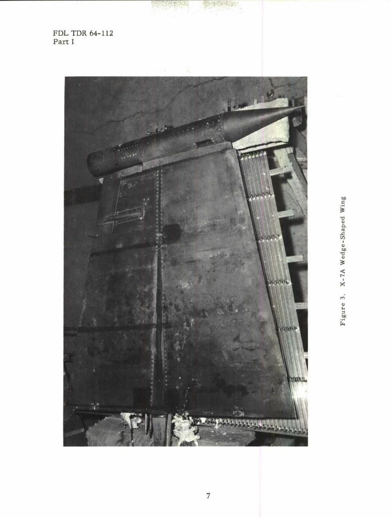
The X-7A wing, shown in Figure 3, was originally designed to investigate the effectsof transient aerodynamic heating on aircraft structures. The leading edge was ground toproduce a knife-edge wedge with an included angle of nine degrees, insulative materialswere applied to some areas, boundary layer trips were installed to produce turbulentflow, and some areas were etched to provide varying degrees of surface roughness.In addition to the skin thermocouples, thermocouples were installed on structuralmembers to determine the internal temperature distribution. Construction details andflight test data are available in Reference 4.

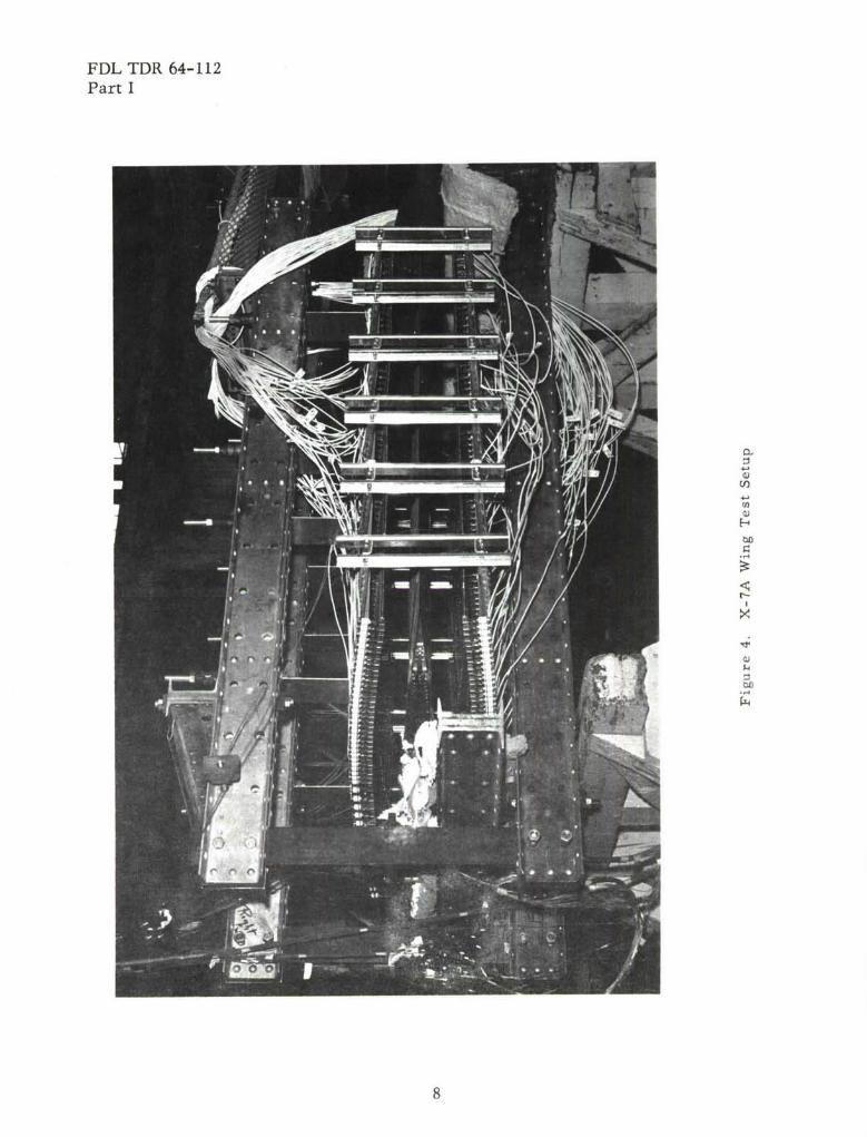
The X-7A wing test setup is shown in Figure 4. The wing was placed between twopolished aluminum reflectors, on which were installed 480 T-3 heating lamps (1000-watt). The wing was divided into eight thermal control areas, four for the top surfaceand four for the lower surface. The maximum skin temperature required was approxi-mately 600OF. Temperatures were measured using the actual flight test thermocoupleswhich consisted of 41 skin and 6 structural thermocouples installed inside the wing.Eight additional thermocouples were installed on the wing external surfaces for computercontrol purposes. The temperature was recorded, reduced and displayed "on-line" bymeans of ETSTF HSDAPS (Elevated Temperature Structural Test Facility's HighSpeed Data Acquisition and Processing System).

CONCLUSIONS

Satisfactory results were obtained in all tests controlled by the General Electric HeatRate Computer. Laboratory temperatures were within 5 percent of the flight recordedtemperatures. This is an acceptable accuracy when it is considered that the informationoriginated with only the flight profile data, the calculations were performed by a digitalcomputer, and the final test was controlled by a closed-loop computer.

The program test results have shown that aerodynamic heating can be accuratelysimulated up to 600*F with radiant heat lamps under computer control. However, someof the areas of original interest still require more study. For example, the temperaturesreached to date are too low to reveal any significant information concerning the effectof using constants in place of temperature dependent variables. Also, in the X-7A wingtest, no attempt was made to cool the wing to the sub-zero temperatures experiencedat the beginning of the test flight. More accurate results would probably have beenobtained if the wing had been initially cooled.

4


4-.

00

5


0.)U)

U)0)H0)

aU0)

0U)z'-40

0)

0)

N

0)

6


7


Ish)

8


Future programs are planned to study simulation techniques to higher temperatureswhere radiation losses and temperature dependent variables become more significant.The test programs will be controlled by a more versatile heat control computer anduse a more elaborate test setup to duplicate the total flight environment as much aspossible. It is anticipated that the information obtained will enable this laboratory toconfidently and accurately simulate aerodynamic heating on any aerospace vehicle.

9

FDL TDR 64-112

Part I

REFERENCES

1. Clark E. Beck. Handbook for Test Engineers (Radiant Heating). Aeronautical SystemsDivision Technical Memorandum, February 1963.

2. General Electric Heat Rate Computer for Wright Air Development Center. Instruc-tion Manual, August 1959.

3. R. B. Snodgrass. Rocket Research Report No. XX, Flight Measurements of Aerody-namic Heating and Boundary-Layer Transition on the Viking 10 Nose Cone. NavalResearch Laboratory Report 4531. June 16, 1955.

4. F. W. Buehl, L. C. Laaksonen, J. M. Lefferde. (UNCLASSIFIED TITLE) X-7Thermal Data Program Final Report. WADD Technical Report 60-567. September1960. (CONFIDENTIAL REPORT)

5. Robert C. Brown, Robert V. Brulle, Gerald D. Giffin. Six-Degree-of-FreedomFlight-Path Study Generalized Computer Program. Part I, Problem Formulation.WADD Technical Report 60-781. May 1961. pp. 89-91, 129-141.

10

FDL TDR 64-112

Part I

APPENDIX I

IBM DIGITAL COMPUTER PROGRAM

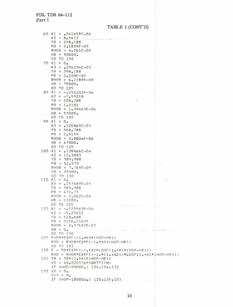
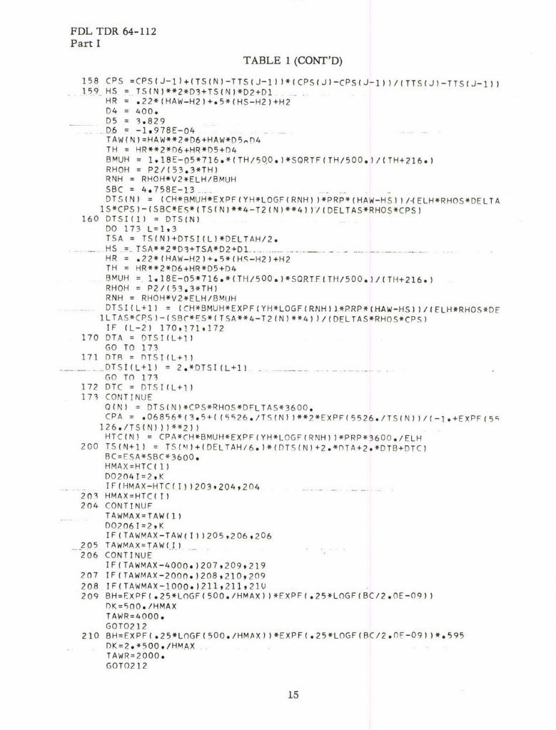
More efficient performance of the many calculations required in this study wereachieved by the digital computer program written for use on the IBM 7094 computer.The program is in the engineers computer language, FORTRAN, and is based on theaerodynamic heating subprogram given in Reference 5. The program shown asTable 1, has been designed to provide information peculiar to the operation of theGeneral Electric Heat Rate Computer used in this laboratory, but it still retains itsFORTRAN style and may be easily utilized by anyone with a knowledge of FORTRANprogramming.

The calculations are based on the aerodynamic heating theory for a thin-skinnedwedge at an angle of attack. By ingoring conduction into the structure, the heat energystored in the skin is considered as the difference between the aerodynamic heat inputand the heat radiated to space. From this theory the following differential equation isderived:

d Ts h (H H) 0 4 Tr4

dt cwrC OW cw S r

where c and c are properties of the skin material and surface condition, and h, C, andH are properties of the air flowing over the point under consideration, All of these

items are functions of the skin temperature. Since the resulting differential equation hasnon-linear coefficients, the Runge-Kutta numerical method is used to obtain the solution.The calculations for determining the heat transfer properties are based upon a referenceenthalpy method, and calculations for determining atmospheric conditions and local flowconditions are based upon the 1959 ARDC Model Atmosphere.

As it is written the digital computer program incorporates the following features:

1. Up to 300 time points for each location on the wedge

2. Altitudes up to 700,000 meters

3. Atmospheric properties calculated according to the 1959 ARDC ModelAtmosphere

4. Provisions for the reading of multiple sets of data with easy variation ofPrandtl Number, critical Reynolds Number, material, and location of eachpoint in question

5. Provisions for a linear interpolation table for variation of material specificheat and emissivity with skin temperature

6. Runge-Kutta method of solving the non-linear differential equation

11


TABLE 1

IBM DIGITAL COMPUTER PROGRAM

c SKIN TEMPERATURE PROGRAMDIMENSION H(nO0),VA(300) ,THETA(300) T,Tci 01) ,DTS,(300),XMN(300) ,T2(3

100) tRN2( 300) ,TTS( 20) ,FS( 20) ,CPS( 20) ,rTSI(4) ,ALFD( 300 ) TAW( 300) ,HTC3(00) ,O( 300) ,TAWP( 300 ) HP( 300) ,TSP( 300)

4 REAPINPUTTAPE2olK1 FORMAT (!3)

- REAr) INPUT TAPE 2929(THFTA(M)tM=1,K)RFAf) INPUT TAPE 792,(H(M),M=1,K)READ INPUT TAPE 2,2,(VA(M),Mt=1,K)READ INPUT TAnF 292q(ALFr)(M),M=I9K)READ INPUT TAPE 2,2#(TTS(M),M=1,20)READ INPUT TAPE 2,2,(CPS(M)qm=1,20)READ INPUT TAPE 2,?,(ES(M),M=1,20).

2 FORMAT (SF13.4)5 READINPUiTTAPF2,3,TS (1) PRPRNCR,07,ELHRHOSDELTASDELTAHESA3 FORMAT (El1.4)

DO 200 N=1,KHGP =.3048*H(N)/( 1.+.3048*H(N)/6156766.)I F (HGP-700000.) 10920,213

10 IF (HGP-200000.) 11,3092011 IF (HGP-170000a) 12,40,3012 IF (HGP-160000*) 13,5904011 IF (HGP-109000.) 14,60,5014 IF (H(7-P-90000,) 15,70,6015 IP (HGP-79000,) 16,80,7016 IF (HGP-53000.) 170,908017 IF (HGP-47000.) 18,10099018 IF (HGP-25000,) 19,110,10019 IF (HGP-11000,) 120,120,11020 Al = .222129F-05

A2 = 9.76137TA = 2816.188PR = 2.9759F1-06RHOB = 6.113E-13H8 = 200000.GO TO 130

30 Al1 = .35O 7 11,E-O5A2 = 6.83296TB = 2566.188PA = 5.8954F-06RHOR = 1.338F-12HB = 170000.C, 0TO 130 -

40 A] = .75414IF-09iA2 = 3.41648T8 = 2386.188PB = 7.5578E-06RHOn = 1*845E-12HA = 160000.G0 TO 130

50 Al = .886289E-04A2 = 1.70824TB = 406.188PB = 1.5562E-04RHOB = 2.212F-10HA = 109000.CV) TO 130

12


TABLE 1 (CONT'D)

60 Al = .241458F-04A2 = 8.5412

TB = 298.188PB = 2.1809F-03RHOB = 4.261E-09HB = 90000oGO TO 130

70 Al = O0

A3 = *206234E-03TR = 298.188PB = 2o108E-0?RHOR = 4.1189F-08H8 = 79000.GO TO 125

80 Al = -. 159202F-04A2 = -7,59218

TB = 508s788PB = 1.2181RHOB = 1.3946qE-06HB = 53000.GO TO 130

90 Al = 0.A3 = .120869E-01TB = 508.788PB = 2.5155RHOB = 2.8804F-06HB = 47000.GO TO 125

100 Al = o138466E-04A2 = 11.3883TB = 389.988PB = 51.979RHOB = 7*765E-05HB = 25000.

GO TO 130110 Al = O0

A3 = .157689E-03TB = 189.988PB = 472.73

RHOB = 7.062E-04HB = 11000.

GO TO 125120 A1 = -. 225569P-04

A2 = -5.25612

TB = 518.688PB = 2116*21615RHOB = 2.37692E-03HB = 0.GO TO 130

125 P=PB*EXPF(-1.*A3*(HGP-HB))RHO = RHOB*EXDFC-1.*A3*(HGP-HRS)GO TO 131

130 P = PB*EXPF(-I,*A2*LOGF(1,+Al*(HGP-HB)))RHO = RHOB*EXPF((-1*(I.+A2).)*LOGF(I,+Al*(HGP-H)))

131 TM = TB*(1,+Al*(HGP-HB))VS = 49*020576*SORTF(TM)IF (HGP-90000.) 134,134.132

132 VS = 0.VT',= 0.IF .(HGP-180000.) 135.135.133

1VDL TDR 64-112Part I

TABLE 1 (CONT'D)

133 IF (HGP-1200000.) 1369213,213134 T = TM

VIS = (T*SQRTF(T)*o0226988E-06)/((T+198*72)*RHO)GO TO 140

135 A =.759511

-8. *174164 ----C =220.

D) 25.GO TO 137

136 A =.935787

Bl * 273966C, -.1804D) 140.

137 T TM*(A-F3*ATANF( (HGP-C)/D))140 IF (VS) 141,141,142141 XMN(N)=0.

GO TO 1431.2XMN (N)I=VA (NI/VS-

ALFHD=F)7+ALFD( N)IF (ALFHD) 143,143,144

143 P2=PR H02 = RHOT2(N) = TV2 =VA(NGO TO 147

144 ALFHR = ALFHr)/57*295CP=2.*ALFHR**')*(.6+SORTF(.36+1./((XMN(N)*ALFHR)**2))).P2=P*(*.7*CP*XMN(FN )**2+1.)RH02=RPO*(6.*02/P+1.,,(6.+P2/P)T2 (N) =T*P2*RHo/(PRH2XMNN=SORTF((6.*P2)7(7.*P,+l.,7.)IF (XMNN/XMN (NJ-I * 146,1.46,143

146 RFTA=ASIN(XMNN/XMN(N))XMN2=(l./SINF(BETA-ALFHR))*SQRTF(5.,(6.**H02/RHO-l.))V2=49.1*XMN2*',ORTF(T?(N))

147 BMU2 1 . 18E-05*716o*(T2(N)/500. )*SQRTF(T2(N)/500. )/(T2(N)+216o)RN2 (N) =RHO2*V2*ELH*32. 174/BMU2IF (RN2(N)-RNCR) 148,149,149

148 CH = .332YH = .5RH = .85GO TO 150

149 CH = o0296YH = o8RH = .9

150 Dl = -94.38D2 = o2331D3 = 8o4E-06H2 = T2(N)**2*03+T2(N)*D2+D1HAW =V2**2*RH/5.012F+04+H2IF( TS(N )-TTS 20 ))151,151,217

11I 0152 1 T +l

IF (TSIN)-TTS(I)) 154,153,192153 ES = ES(I)

GO TO 155154 FS =FS(1-1)+(TS,(N)-TTS( 1-1) )*(ES(! )-FSUI-1))/(TTS,(I )-TTS,(I-1))155 J =0

156 J =J+i

IF (TS;(N)-TTS(J)) 158,157,156157 CPS = CP5(J)

GO TO 159

14


TABLE 1 (CONT'D)

158 CPS =C S J 1+ T ( )T S J 1 ) (P (J -P ( - )/ T S J -T ( - )159- HS =_.TS(N)**2*D3+TS(N)*D2+D1

HR = .22*(HAW-H2)+*5*(HS-H2)+H2D4 = 400.D5 = 3.829_6= -1*978E-04

TAW (N) =HAW**2*D6+HAW*D5,44TH = HR**2*r)6+HR*D5+D4BMUH = 1.18E-05*716.*('TH/5QO.O)*SQRTFcTH/500.)/(TH+216.)RHOH = P2/(53.3*TH)RNH =RHOH*V2*ELH/BMUHSBC =4*758E-13--DTS(N) = (CH*BMUH*EXPF(YH*LOGF(RNH) )*PRP*(HAW-HS))/.(ELH*RHOS*DELTA1S*CPS)-(SBC*Es*(TS(N)**4-T2(N)**4))l/(DELTAS*RHOS*CPS)

160 DTSI(1) =DTS(N)DO 173 L=193TSA =TS(N)+DTSI(L)*DELTAH/2.

-- SHS TSA**2*DI+TSA*D2+Dl..,....--*-HR = 22*(HAW-H2)+*5*(H,)-H2)+H2TH HR**2*D6+HR*D5+D48MUH =. 1.18E-05*716.*(TH/500.)*SQRTF(TH,/500.)/(TH+216.,RHOH =P2/(53,3*TH)

RNH =RHOH*V2*ELH/BMLIH

DTSI(L+l) =((CH*BMUH*EXPFCYH*LOGF(RNH)).*PRP*(HAW-.HS) )/tFLH*RHOS*DFlLTAS*CPS)-(SB-*P-S*cTSA**4-T2(N)**4) )/(DELTAS*RHOS*CPS)IF (L-2) 17091719172

170 OTA = DTSI(L+1)GO rO 173

171 DTR = TSI(L+l)-DTS I(L+l ) = 2 .*DTS I(L+lGO TO 173

172 DTC = DTSI(L+1)173 CONTINUE

0(N) =DTS(N)*CPS*RHOS*DFLTAS*3600.

CPA .O6856*(3.54U(5926./Ts(N)l**2*EXPF(5526./TS(N)),.c-1.+EXPF(5'1269/TS(N) I)**2))HTC(N) =CPA*CH*BMUH*EXPF(YH*LOGF(RNH, )*PRP*3600.,ELH

200 TS(N+1) =TS(k')+(DELTAH/6. )*(DTS(N)+2.*nTA+2.*DTB+DTC)BC=FSA*SBC* 3600.HMAX=HTC( 1)D02041=29KIF(HMAX-HTC(1l)2039204,204

203 HMAX=HTC(T)204 CONTINUF

TAWMAX=TAW( 1)D02061=2, KIF( TAWMAX-TAW( I) )205#2 069,206

-2 *05 TAWMAX=TAW(.I.)206 CONTINUE

IF(TAWMAX-4000. )207,209,219207 TF(TAWMAX-2000*)2089210,209208 TF(TAWMAX-1000. 1211 ,211*21V209 BH=EXPF(.25*LoGF(500./HMAX))*FXPF(.25*LOGF(BC/2.OE-09))

DK=900. /HMAXTAWR=4000*GOT0212

210 BH=FXPF( .25*LOGF(500./HMAX) )*EXPF(.25*LOGF(BC/2eOE-09) )**595DK=2.*500./HMAX.TAWR= 2000.GOT0212


TABLE 1 (CONT'D)

211 RH=EXPF(.25*LOGF(500./HMAX))*EXPF(.25*LOGF(8C/2.OE-09))*.354DK=4.*500. /HMAXTAWR= 1000.

2 12 IS-.MA -X=T5( 1) .- - - - - -

DO2251T=2, KTF( TSMAX-TS (TIl 224t,225 ,2?

224 TSMAX=TS(T)225 CONTINUE

IF(TSMAX-4000. ) 26?28 ,21 9226- IF(T-SMAX-2000.)22.7.22922?8227 IF( TSMAX-1000. )230,230,229228 TSR=4000.

G0T0231??P TSR=?000.

GOT0231

210 T5R.=1000.------211 DO23?T=19K

TSP (I) =TS (I 1*99.5/TSRTAWP( I)=TAW( I)*99*5/TAWR

232 HP(T)=HTCfT)*Q9.5/HMAXWR ITFO)JTPUTTAPF19220, FLH

--,.--22OJTODRMALAI-IHA,1X25HELH =tEl1.4,).....-222 WRITFOUTPUTTAPE39223tBH221 FORMAT (2X*5HRH =9E11.41

WR ITEOIJTPUTTAPE3 ,2339DK233 FORMAT (2Xs9HrnK =,F11.4)

WRITEOUJTPUTTAPE3,201 ( THFTAC I) H(I) ,VA (I) ALFD( I) ,XMN CI) ,TS(I)g1)TS,(I),TAW(fl),T2(IflRN2(1),I=1,K)

201 FORMAT (3X;8HTIME=SEC,6X,6HALT=FT,5X,7HVEL=FP5ý,5X,8HALFD=DEG,7X ,2HIMN,9X,4HTS=R,.6X,7HOTS=RPS,6X,5HTAW=Ri,8X,4HT2=R,8X,3HRN2/1HA,1OE 12.

WR TTFOUJTPUTTAPE3, 202 1 THFTA( I) ,HTC( I) ,O(1ITAWP( I) ,HP( I) ,TSP (1)1,1 =1 9 K)

202 FORMAT(lHA,2X,8HTTMF=SEC,7X,3HHTC,1OX,lHQ,1OX,4HTAWP,9X,2HHP,9X,3IHTS'P/lHA96E12*4/(IX,6F12.4))C1OTn5

219 WRITFOLJTPUTTADE3,22 1

221 FORMAT (23H TAW OR TS O)UT OF RANGE)CO To?2 1 5

211 WRITF OUTPUT TAPF !,?14

214 FORMAT (2P,01 HAýLlI TIDFý OUIT Qf7 RANrE)(30 TO 215

217 WR IT FnuT - JT T A rýF 118218 FORMAT(40H SýKTN TFMDFRATflRF FXCEFDS) RANGE OF TABLE)215 CALL FXIT

216 FNn

16

FDL TDR 64-112

Part I

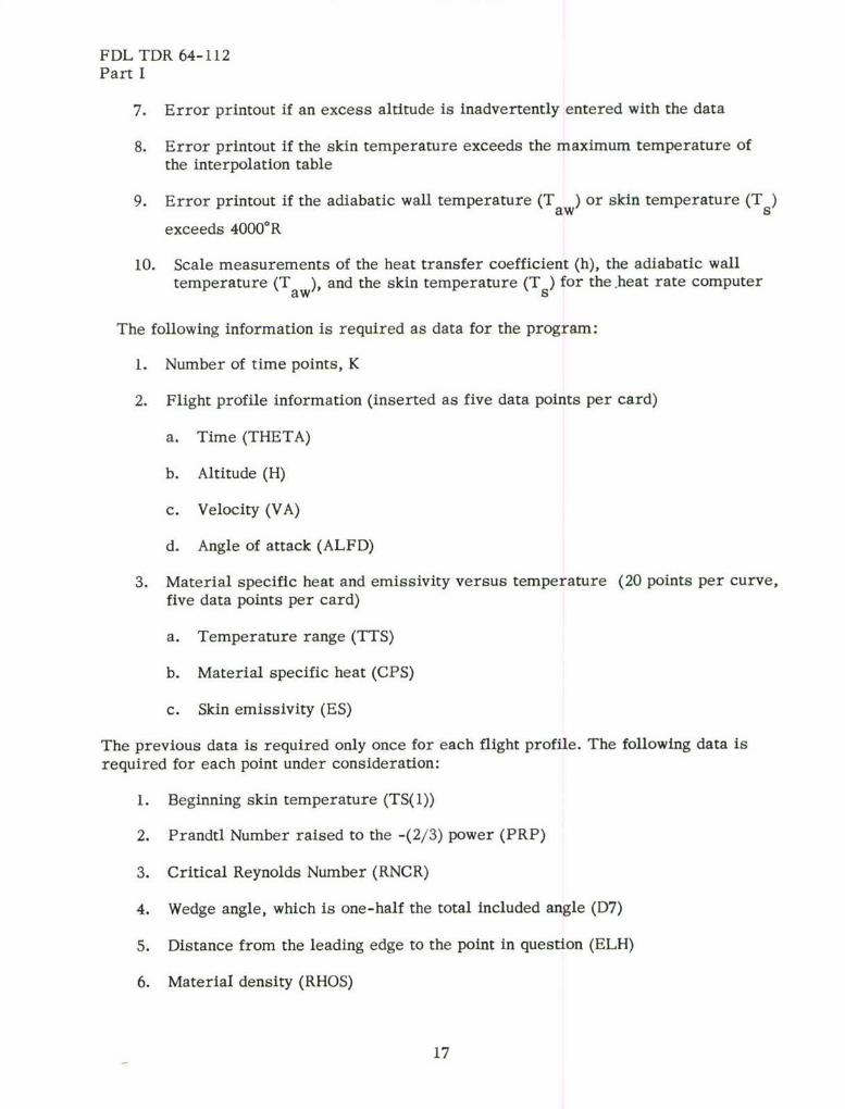
7. Error printout if an excess altitude is inadvertently entered with the data

8. Error printout if the skin temperature exceeds the maximum temperature ofthe interpolation table

9. Error printout if the adiabatic wall temperature (T aw) or skin temperature (T s)

exceeds 4000'R

10. Scale measurements of the heat transfer coefficient (h), the adiabatic walltemperature (Taw), and the skin temperature (Ts) for the .heat rate computer

The following information is required as data for the program:

1. Number of time points, K

2. Flight profile information (inserted as five data points per card)

a. Time (THETA)

b. Altitude (H)

c. Velocity (VA)

d. Angle of attack (ALFD)

3. Material specific heat and emissivity versus temperature (20 points per curve,five data points per card)

a. Temperature range (TTS)

b. Material specific heat (CPS)

c. Skin emissivity (ES)

The previous data is required only once for each flight profile. The following data isrequired for each point under consideration:

1. Beginning skin temperature (TS(l))

2. Prandtl Number raised to the -(2/3) power (PRP)

3. Critical Reynolds Number (RNCR)

4. Wedge angle, which is one-half the total included angle (D7)

5. Distance from the leading edge to the point in question (ELH)

6. Material density (RHOS)

17

FDL TDR 64-112

Part I

7. Material thickness (DELTAS)

8. Time increment (DELTAH)

9. Average skin emissivity for expected temperature range (ESA)

The results of the computer program are printed in tabulated form with headings atthe top of each column. The following results are printed adjacent to the correspondingtime:

1. Time

2. Altitude

3. Velocity

4. Angle of attack

5. Local Mach Number

6. Skin temperature

7. Derivative of skin temperature with respect to time

8. Adiabatic wall temperature

9. Local atmospheric temperature aft of the shock wave

10. Local Reynolds Number aft of the shock wave

11. Heat transfer coefficient

12. Total heat transferred

13. Paper tape punch values for the adiabatic wall temperature, skin temperature,and the heat transfer coefficient

The tabulated results are headed by a printout of the location of the point in question,the B-h potentiometer setting, and the demand gain. All results are given to foursignificant digits.

The information obtained from the digital computer program is used to design thelaboratory test setup for simulating the aerodynamic heating. The heat transferred andthe tempature rise rate are used to determine power requirements, and the heattransfer coefficient and the adiabatic wall temperature are used as inputs to the heat ratecomputer.

18

FDL TDR 64-112

Part I

APPENDIX II

SPECIAL PURPOSE HEAT RATE COMPUTER

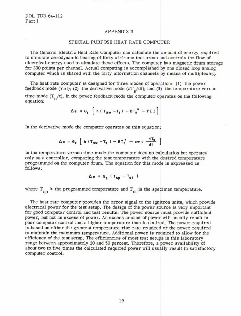
The General Electric Heat Rate Computer can calculate the amount of energy requiredto simulate aerodynamic heating of forty airframe test areas and controls the flow ofelectrical energy used to simulate these effects. The computer has magnetic drum storagefor 300 points per channel. Actual computing is accomplished by one closed loop analogcomputer which is shared with the forty information channels by means of multiplexing.

The heat rate computer Is designed for three modes of operation: (1) the powerfeedback mode (YEI); (2) the derivative mode (dTs/dt); and (3) the temperature versus

time mode (T s/t). In the power feedback mode the computer operates on the followingequation:

A = GI [ h(Tow--Ts) -- BT, -- YE:]

In the derivative mode the computer operates on this equation:

Ae = G2 h (Tow -Ts )-BT4 -- cwr" dT-t-3 dt

In the temperature versus time mode the computer does no calculation but operatesonly as a controller, comparing the test temperature with the desired temperatureprogrammed on the computer drum. The equation for this mode is expressed asfollows:

A: G (Tsp -Tst )

where Tsp is the programmed temperature and Tst is the specimen temperature.

The heat rate computer provides the error signal to the ignitron units, which provideelectrical power for the test setup. The design of the power source is very importantfor good computer control and test results. The power source must provide sufficientpower, but not an excess of power. An excess amount of power will usually result inpoor computer control and a higher temperature than is desired. The power requiredIs based on either the greatest temperature rise rate required or the power requiredto maintain the maximum temperature. Additional power is required to allow for theefficiency of the test setup. The efficiencies of most test setups in this laboratoryrange between approximately 20 and 50 percent. Therefore, a power availability ofabout two to five times the calculated required power will usually result in satisfactorycomputer control.

19

"FDL TDR 64-112

Part I

SCALING

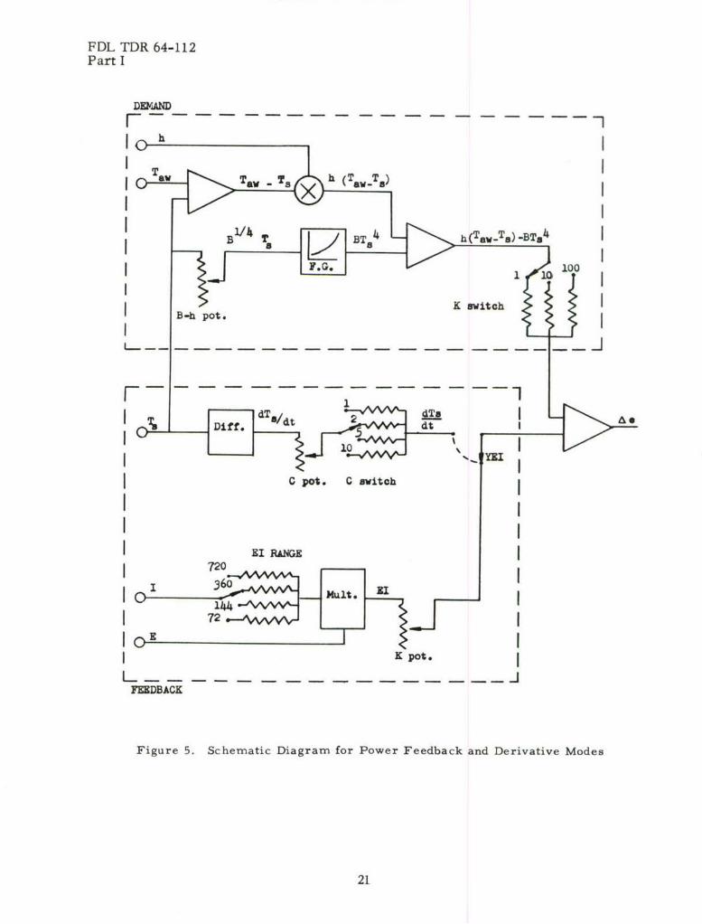
In the power feedback (YEI) and derivative (dTs/dt) modes the computer operatesin a closed loop which consists of a demand side and a feedback side. The demand sideis represented by the following portion of the design equations:

h (T 0 -Ts )-TBT 4

dTsThe feedback side is represented by YEI for the power feedback mode, and cwr dt

for the derivative mode. Both sides of the closed loop must be scaled properly forsatisfactory test results. A schematic diagram of the power feedback and derivativemodes is shown in Figure 5.

DEMAND SCALING

The demand scaling is identical for both the power feedback mode (YEI) and thederivative mode (dTs/dt). The factors involved are the heat transfer coefficient curve(h), the adiabatic wall temperature curve (Taw), the B-h SCALE FACTOR potentiometer,

the skin temperature range selector switch, the thermocouple selector switch, the KSCALE FACTOR switch, the power range selector switch, and the mode selector switch.

The mode selector switch has three positions: (1) EI, for power feedback mode,(2) dTs/dt, for derivative mode, and (3) Ts/t, for the temperature versus time mode.

The thermocouple selector switch is set to correspond with the type of thermocoupleused on the test specimen. Positions are available for thermocouples of: Iron-Constantan;Chromel-Constantan; Chromel-Alumel; and Platinum -Platinum, 10-percent Rhodium.

The skin temperature range selector switch has positions of 10000, 20000, and 40000R.This switch should be set on the closest range that exceeds the maximum adiabatic walltemperature stored on the drum or the maximum skin temperature, whichever isgreatest.

The K SCALE FACTOR switch has settings of 1, 10, and 100 available. Althoughthis switch is usually left at a setting of 1, it may be used to obtain more demand gainthan is available in the inherent gain obtained in the scaling of the h and Taw curves.

The El RANGE switch has settings that represent an electrical load of 72, 144, 360,and 720 KW. In the derivative mode (dTs/dt) this switch has no control feature and itshould be set at the nearest range that exceeds the connected load when the full voltage(580 volts) is applied. Each power range also has a gain associated with it. These gainsare important in the power feedback mode (YEI), where the EI RANGE switch is a partof the feedback mode circuitry. The manipulation of this switch in the power feedbackmode will be discussed in the section on feedback scaling.

20


DEMAND

T h(TB TaT8 ) T3

3 X (T A

I- pot..aith

I .5I Z I

I Ell RANGEI

FUDBACK

Figure 5. Schematic Diagram for Power Feedback and Derivative Modes

21


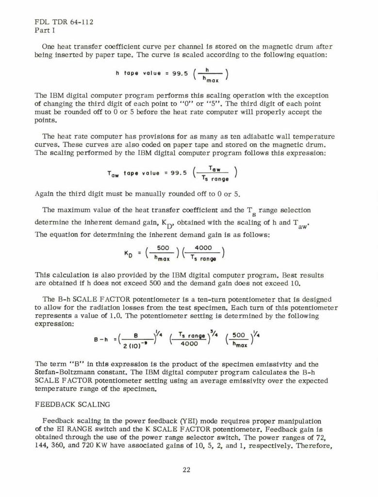
One heat transfer coefficient curve per channel is stored on the magnetic drum afterbeing inserted by paper tape. The curve is scaled according to the following equation:

h tape value = 99.5 ( h )max

The IBM digital computer program performs this scaling operation with the exceptionof changing the third digit of each point to "0" or "5". The third digit of each pointmust be rounded off to 0 or 5 before the heat rate computer will properly accept thepoints.

The heat rate computer has provisions for as many as ten adiabatic wall temperaturecurves. These curves are also coded on paper tape and stored on the magnetic drum.The scaling performed by the IBM digital computer program follows this expression:

Tow tape value = 99.5 (TowT range

Again the third digit must be manually rounded off to 0 or 5.

The maximum value of the heat transfer coefficient and the T5 range selection

determine the inherent demand gain, K obtained with the scaling of h and Taw

The equation for determining the inherent demand gain is as follows:

h0 4000

hD max Ts rango

This calculation is also provided by the IBM digital computer program. Best resultsare obtained if h does not exceed 500 and the demand gain does not exceed 10.

The B-h SCALE FACTOR potentiometer is a ten-turn potentiometer that Is designedto allow for the radiation losses from the test specimen. Each turn of this potentiometerrepresents a value of 1.0. The potentiometer setting is determined by the followingexpression:

B-h A 2s ( srang!)o4 500Y= -4000 hmax

The term "B" in this expression is the product of the specimen emissivity and theStefan-Boltzmann constant. The IBM digital computer program calculates the B-hSCALE FACTOR potentiometer setting using an average emissivity over the expectedtemperature range of the specimen.

FEEDBACK SCALING

Feedback scaling In the power feedback (YEI) mode requires proper manipulationof the EI RANGE switch and the K SCALE FACTOR potentiometer. Feedback gain isobtained through the use of the power range selector switch. The power ranges of 72,144, 360, and 720 KW have associated gains of 10, 5, 2, and 1, respectively. Therefore,

22


the required gain, as well as the required power, must be considered in arriving at thepower setting of the El RANGE switch. The utilization of this switch will be discussed inthe scaling examples.

The K SCALE FACTOR potentiometer is a ten-turn potentiometer with each rotationof the dial representing a value of 0.1. This potentiometer is used to attenuate thefeedback signal to allow for the efficiency of the test setup. When the power rangeselector switch is set so the feedback gain is the same as the demand gain, the settingfor the K SCALE FACTOR potentiometer is the efficiency of the channel (??) dividedby the area (A) covered by the channel. However, the EI RANGE switch and the K SCALEFACTOR potentiometer may be combined in such a way that almost unlimited values offeedback gain may be obtained. The combination of these two controls is covered in thescaling examples.

In order to arrive at the proper K SCALE FACTOR potentiometer setting, the efficiencyof the test setup must be known. This efficiency is usually determined by a constantpower efficiency test. This test may be run on a simulated test setup, but should beconducted on the actual test setup, if feasible. The efficiency test should be designed torequire a constant power that will give a specimen temperature rise rate that iscomparable to that expected in the actual simulation test.

The efficiency test is conducted in conjunction with the data processing system.The data section has a program written for the CDC 1604 digital computer based on thefollowing equation:

71_ (1.0542

This equation is legitimate as long as it is applied to a portion of the temperature curvewhere the rise rate is relatively constant. To prepare the efficiency program, the datasection must be provided the following information: material thickness (r), materialdensity (w), a curve of material specific heat versus temperature, thermocouple type,and the power range to be used. The 1604 computer is then operated on-line with theheat rate computer to provide the temperature, temperature rise rate, power absorbedby the specimen, total power required, and the efficiency per unit area. The efficiencyper unit area is then used in setting the K SCALE FACTOR potentiometer.

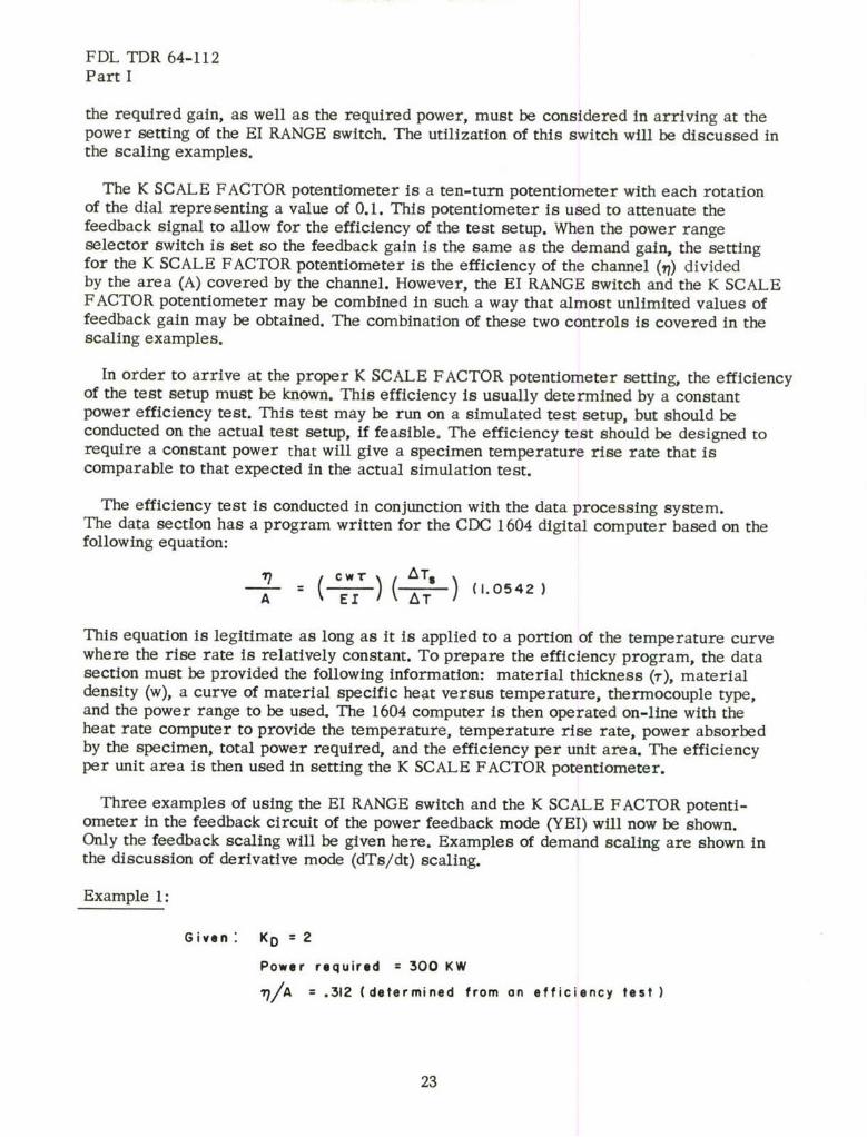
Three examples of using the El RANGE switch and the K SCALE FACTOR potenti-ometer in the feedback circuit of the power feedback mode (YEI) will now be shown.Only the feedback scaling will be given here. Examples of demand scaling are shown inthe discussion of derivative mode (dTs/dt) scaling.

Example 1:

Given: KD = 2

Power required = 300 KW

77/A = .312 (determined from an efficiency test)

23


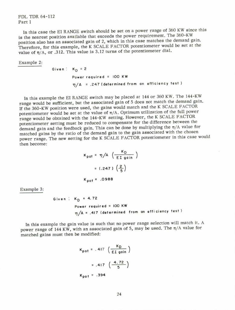
In this case the El RANGE switch should be set on a power range of 360 KW since this

is the nearest position available that exceeds the power requirement. The 360-KW

position also has an associated gain of 2, which in this case matches the demand gain.

Therefore, for this example, the K SCALE FACTOR potentiometer would be set at the

value of 77/A, or .312. This value is 3.12 turns of the potentiometer dial.

Example 2:

Given " KD = 2


V/A = .247 (determined from an efficiency test

In this example the El RANGE switch may be placed at 144 or 360 KW. The 144-KW

range would be sufficient, but the associated gain of 5 does not match the demand gain.

If the 360-KW position were used, the gains would match and the K SCALE FACTOR

potentiometer would be set at the value of n/A. Optimum utilization of the full power

range would be obtained with the 144-KW setting. However, the K SCALE FACTOR

potentiometer setting must be reduced to compensate for the difference between the

demand gain and the feedback gain. This can be done by multiplying the 17/A value for

matched gains by the ratio of the demand gain to the gain associated with the chosen

power range. The new setting for the K SCALE FACTOR potentiometer in this case would

then become:

Kpot "7/A / (TgEl gain

= (.247) 2*-

Kpot = .0988

Example 3:

Given . KD = 4.72


-n/A = .417 (determined from an effi ciency test

In this example the gain value is such that no power range selection will match it. A

power range of 144 KW, with an associated gain of 5, may be used. The 77/A value for

matched gains must then be modified:

Kpot .41T KD )o El gain

- .417 ( 4"72 )

Kpot .394

24


A general expression for finding the proper K SCALE FACTOR potentiometer settingcan be derived from the previous examples. This expression is:

17/ KDKPt A (El gain)

where EI gain is the associated gain of the chosen power range. This equation may beused as long as the calculated value does not exceed 1.0. For instance if the demandgain is 5 and the t/A is .25, the El RANGE switch may be set at 360 KW, or a gainof 2. The potentiometer setting would then become:

Kpot = (.25)( 5

Kpot = .625

However, under these conditions the El RANGE switch could not be placed at 720 KW, ora gain of 1, because the potentiometer setting would then become:

Kp o t= (.25) (-5)

Kpot = 1.25

which is impossible to set on the potentiometer. Therefore, the power range and thedemand gain must be combined in a way such that the K SCALE FACTOR potentiometercalculation does not exceed 1.0.

The feedback scaling for the derivative mode (dTs/dt) is very similar to that of thepower feedback mode. In the derivative mode the C SCALE FACTOR switch and the CSCALE FACTOR potentiometer are used to obtain the required feedback gain. The CSCALE FACTOR switch is a four-position switch with gain settings of 1, 2, 5, and34.125*. The C SCALE FACTOR potentiometer is a ten-turn potentiometer with eachrotation of the dial representing a value of 1.0. When the C SCALE FACTOR switch isset on a gain that matches the demand gain, the proper setting for the C SCALE FACTORpotentiometer is cwr. However, the C SCALE FACTOR switch and the C SCALEFACTOR potentiometer can be combined to give almost any value of feedback gain. Theuse of these two controls is discussed in the scaling examples.

*This gain is obtained by setting the C SCALE FACTOR switch at 10. The switch was

originally designed with a gain of 10, but a resistor was changed during computermodifications to give the new gain of 34.125. This position is now Intended for thetemperature versus time mode only, but it may still be used in the derivative mode.

25


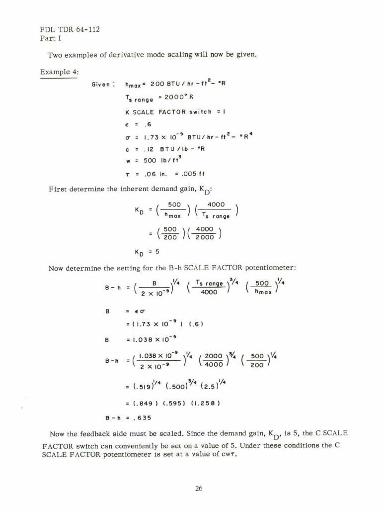
Two examples of derivative mode scaling will now be given.

Example 4:

Given: hmax= 200 BTU/ hr -ftt 2 - 'R

"Ts range = 20000R

K SCALE FACTOR switch = I

e .6

"r= 1.73 X 10-9 BTU/hr-ft2 - 'R 4

c = .12 BTU/ib-*R

w = 500 lb/ft3

T .06 in. = .005 ft

First determine the inherent demand gain, KD

I 500 4000Shmax Ts range

S/500 400020 2 000

KD 5

Now determine the setting for the B-h SCALE FACTOR potentiometer:

B /'4 Ts range_)3/i ( 500 )1/4B- h 2 x 10-'/ 4000 hmax

B E 0o

( 1I.73 X 10- 9 ) (.6)

B = 1.038 X 10-9

B-h 1.038 X 10-' )Y 2000 V/4 500 )'/4

2 X10 ) (4ooo0 200

5 .19)' /4 (.500)3/4 (2.5)1/4

= (.849 ) (.595) (1.258)

B-h .635

Now the feedback side must be scaled. Since the demand gain, KD" Is 5, the C SCALE

FACTOR switch can conveniently be set on a value of 5. Under these conditions the CSCALE FACTOR potentiometer is set at a value of cw".

26


Cpot =cwr•p (12) ( 500) (.005)

Cpt.300

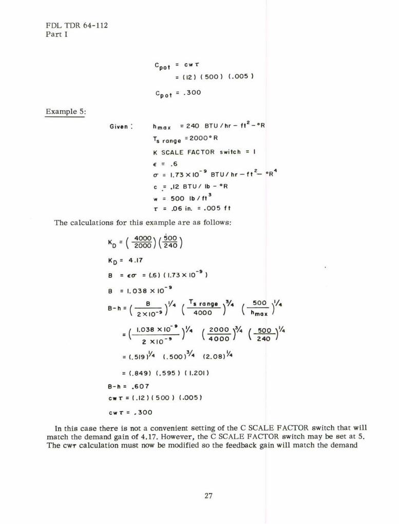
Example 5:

Given hmax 240 BTU /hr- ft 2 °R

Ts range =200 0 °R

K SCALE FACTOR switch = I

E .6

- =1.73 X10- BTU/hr--ft OR4

c = .12 BTU/ lb - OR

w= 500 lb/ft3

= .06 in. .005 ft

The calculations for this example are as follows:

K= 4000 0 600D= 2000 240

KD = 4.17

B = for = (.6) (I.73X10-)

B = 1.038 X 10- 9

B 1/4 Tsrange / 4 (500/4"( oo""")/"2XI()("m,,a°/

= (.0 o"~0 )'/4 (2000 )°° (' •500 )l'

= (.5I9)',, C.5o0015,, (2.08).,

= (.849) (.595) (I.20I)

B-= .607

cwr 1 (.IX)(500) (.005)

cw r= . 300

In this case there is not a convenient setting of the C SCALE FACTOR switch that willmatch the demand gain of 4.17. However, the C SCALE FACTOR switch may be set at 5.

The cwr calculation must now be modified so the feedback gain will match the demand

27

"FDL TDR 64-112Part I

gain. This can be done by multiplying cwr by the ratio of the demand gain to the C SCALEFACTOR switch position. Therefore, the setting for the C SCALE FACTOR potentiometerwill be:

CPO ~cw r(KDCpot= cT (Cswitch

=() ( 4.17)' 5

Cpot =.250

The C SCALE FACTOR switch could also be set at 1. In this case the C SCALEFACTOR potentiometer setting would be:

Cpo0 = (.30) (-. )

Cpot = 1.251

From the two previous examples the following general expression can be derivedfor determining the setting for the C SCALE FACTOR potentiometer:

CPO =CWT (KD

Cswitch )

This expression may be used as long as the calculated setting does not exceed 10.

TEMPERATURE VS. TIME MODE

In the temperature versus time mode the heat rate computer is used only as a controller.The error signal is obtained from the difference between the programmed temperature andthe specimen temperature. The error signal is proportional to the amount the specimentemperature drops below the desired temperature. The following proportional bands areavailable for the appropriate temperature range:

Scale Proportional Bands

10000R 10, 20, 30, 40, 50, 60, 70, 80, 90, 100'R

20000R 20, 40, 60, 80, 100, 120, 1.40, 160, 180, 200-R

4000OR 40, 80, 120, 160, 200, 240, 280, 320, 360, 400-R

Each proportional band figure means that a specimen temperature lag of that value willresult in the full error signal of 50 volts.

The power arrangement is extremely important in the temperature versus time mode.The temperature program should be designed so that no step increment will requiremore than one-fourth of the total available load. This means that for smooth computercontrol the ratio of the power output per volt of Ae should be held to a minimum. A

28


proportional band should be chosen such that the maximum step increment will demandnot more than one-half kilowatt per lamp. If this proportional band is unsatisfactory,some trial runs may be necessary to decide which proportional band gives the bestcombination of good test results and smooth control.

The demand signal in the temperature versus time mode is obtained in the scaling ofthe specimen temperature by the digital computer program. The skin temperature isscaled according to the following equation:

Ts tape value = 99.5 ( Ts

range

As in the previous cases the third digit of each point must be rounded off to 0 or 5.

The only controls in the feedback circuit of the temperature versus time mode arethe C SCALE FACTOR potentiometer and the C SCALE FACTOR switch. With the KSCALE FACTOR switch in the demand side set at 10, and the C SCALE FACTOR switchset at a gain of 34.125*, the computer technicians set the C SCALE FACTOR potentiome-ter so that a temperature lag equal to the chosen proportional band will result in an errorsignal of 50 volts. This is accomplished by first inserting the maximum desired tempera-ture in the demand circuit. A millivolt signal is then manually inserted in the feedbackcircuit to represent the thermocouple signal equal to the maximum desired temperatureminus the chosen proportional band. The C SCALE FACTOR potentiometer is thenadjusted until the error signal is 50 volts. The demand and feedback circuits are nowconsidered "balanced."

To eliminate any lag in the temperature versus time mode, the amount of demand mustbe increased. This may be done in one of two ways. (1) each point of the demand curvemay be multiplied by this factor:

Ts max + P.O. Offset

Ts max

Or, (2) the C SCALE FACTOR potentiometer setting at balanced conditions may bedivided by this factor:

TsmaxTs max -P.B.Offset

The proportional band offset may be determined from the power arrangement. However,if the calculated value does not give satisfactory test results, a new proportional bandoffset can be easily inserted by using the second method.

*This gain is obtained by setting the C SCALE FACTOR switch at the indicated value 10.

29


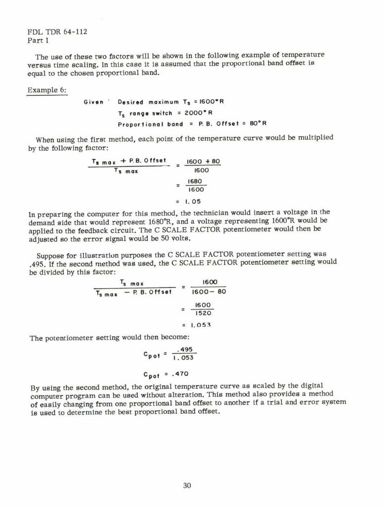
The use of these two factors will be shown in the following example of temperature

versus time scaling. In this case it is assumed that the proportional band offset is

equal to the chosen proportional band.

Example 6:

Given Desired maximum Ts =1600*R

Ts range switch = 2000R

Proportional bond = P.B. Offset = 80R

When using the first method, each point of the temperature curve would be multiplied

by the following factor:

Ts max + P.B. Offset 1600 +80Ts max 1600

1680

1600

1.05

In preparing the computer for this method, the technician would insert a voltage in the

demand side that would represent 1680R, and a voltage representing 1600OR would be

applied to the feedback circuit. The C SCALE FACTOR potentiometer would then beadjusted so the error signal would be 50 volts.

Suppose for illustration purposes the C SCALE FACTOR potentiometer setting was

.495. If the second method was used, the C SCALE FACTOR potentiometer setting would

be divided by this factor:Ts max 1600

Ts max - P B. Offset 1600- 80

16001520

- 1.053

The potentiometer setting would then become:

C~ .495

CPt -1.053

Cpot= .470

By using the second method, the original temperature curve as scaled by the digital

computer program can be used without alteration. This method also provides a method

of easily changing from one proportional band offset to another if a trial and error system

is used to determine the best proportional band offset.

30

aerodynamic heating simulation. part 1. theory and program definition

Documents