aerodynamic heating around flare-type membrane … · instructions for use title aerodynamic...

Instructions for use

Title Aerodynamic Heating Around Flare-Type Membrane Inflatable Vehicle in Suborbital Reentry Demonstration Flight

Author(s) Takahashi, Yusuke; Yamada, Kazuhiko; Abe, Takashi; Suzuki, Kojiro

Citation Journal of spacecraft and rockets, 52(6): 1530-1541

Issue Date 2015-11

Doc URL http://hdl.handle.net/2115/60702

Rights © 2015 American Institute of Aeronautics and Astronautics

Type article (author version)

File Information journal_SMAAC-heatflux.pdf

Hokkaido University Collection of Scholarly and Academic Papers : HUSCAP

https://eprints.lib.hokudai.ac.jp/dspace/about.en.jsp

Aerodynamic Heating around Flare-type MembraneInflatable Vehicle in Suborbital Reentry Demonstration

Flight

Yusuke Takahashi1

Hokkaido University, Kita 13 Nishi 8, Kita-ku, Sapporo, Hokkaido, 060-8628, Japan,Kazuhiko Yamada2, Takashi Abe3,

Japan Aerospace Exploration Agency, 3-1-1 Yoshinodai Chuo-ku, Sagamihara, Kanagawa252-5210, Japan

andKojiro Suzuki4

The University of Tokyo, 5-1-5 Kashiwanoha, Kashiwa, Chiba, 277-8561, Japan

Abstract

A demonstration flight of an advanced reentry vehicle was carried out using a sound-ing rocket. The vehicle was equipped with a flexible (membrane) aeroshell deployedby an inflatable torus structure. Its most remarkable feature was the low ballisticcoefficient that enables reduction in aerodynamic heating and deceleration at a highaltitude. During the suborbital reentry, temperatures at several locations on a backsideof the flexible aeroshell and inside the capsule were measured by means of embeddedthermocouples. The aerodynamic heating behavior of the vehicle was investigated us-ing the measured temperature history, in combination with a numerical prediction inwhich a flow-field simulation of the heating was conducted. In this flow-field simulation,both laminar flow and turbulent flow were assumed, and the deformation of the flexibleaeroshell was considered. A thermal model of the capsule and membrane aeroshell wasdeveloped, and the heat flux profiles of the vehicle surface during aerodynamic heatingwere constructed based on the measured temperatures. The measured temperaturedata were found to be in reasonable agreement with the predicted data if the flow fieldnear the capsule of the vehicle was assumed to be laminar, with a transition to turbulentflow near the membrane aeroshell.

Nomenclature

a = coefficientCp = specific heat at constant pressure, J/(kg·K)E = Young’s modulus, Pah = heat transfer coefficient W/(m2 ·K), or membrane thickness, mIsolar = solar constant, W/m2

k = turbulent kinetic energy J/kgl, L = length, mns = number of speciesnm = number of moleculesNu = Nusselt numberp = pressure, Pa

1Assistant Professor, Faculty of Engineering; [email protected] Professor, Institute of Space and Astronautical Science.3Professor, Institute of Space and Astronautical Science.4Professor, Graduate School of Frontier Sciences.

1

Pr = Prandtl numberq = heat flux, W/m2

R = gas constant, J/(kg·K)Re = Reynolds numberr = position vector, mS = membrane area, m2

t = time, sT = temperature, KU = velocity, m/sε = emissivity, or strainΘvib,s = vibrational characteristic temperature, Kκ = Heat conductivity, W/(m ·K)ρ = density, kg/m3

µ = viscosity, Pa·sν = Poisson’s ratioσ = Stefan-Boltzmann constant

Subscriptsatm = atmosphereb = backgroundconv = convectionsolar = solart = turbulent∞ = freestream

1 Introduction

A reentry vehicle with a membrane aeroshell deployable by an inflatable torus structure isa candidate for a next generation space transport system. The main feature of note for thiskind of vehicle, which was originally proposed in the 1960s, is the low ballistic coefficientduring atmospheric reentry. Since then, several studies and demonstration flights have beenperformed by the National Aeronautics and Space Administration (NASA), the EuropeanSpace Technology (ESA), and the Japan Aerospace Exploration Agency (JAXA). In general,the use of a deployable aeroshell allows the vehicle to be decelerated at a higher altitudecompared with a conventional rigid reentry vehicle. This provides several advantages for theentry, descent, and landing (EDL) approach, such as a lower heat load from aerodynamicheating and reduction in radio-frequency blackout [1–9].

Recently, a reentry vehicle with an inflatable aeroshell has also been developed in theMembrane Aeroshell for Atmospheric-entry Capsule (MAAC) project, in cooperation withseveral universities and JAXA. In the considered reentry mission, a capsule with a tightlypacked aeroshell, e.g., a slender cylinderical shape, is first transported to a given orbit.As the torus tube is inflated, the vehicle rapidly expands the membrane aeroshell undervacuum and microgravity conditions. After deployment, the flare-type membrane aeroshellis sustained by an inflatable torus. It should be noted that the deployed aeroshell later playsroles as a parachute and float after splashing. Then, the vehicle is kicked into an atmosphericreentry orbit. Because of the large area and light weight of the aeroshell, the vehicle canachieve a low-ballistic-coefficient flight during atmospheric reentry. This kind of inflatable

2

deceleration system may not require a parachute because of its low terminal velocity uponlanding. Additionally, because the aeroshell deployment is accomplished before deorbit, acritical operation, such as parachute extraction, is possibly dispensed in exchange for the useof the inflatable vehicle during the EDL approach.

Some studies and the development of elemental technologies for a future inflatable vehiclehave been experimentally and numerically performed as part of the MAAC project. Thebasic concept of a low-ballistic-coefficient flight for the MAAC results in a reduction in theaerodynamic heating. This directly contributes to a decrease in the heat flux on the surface ofthe vehicle. Free flight tests using a scientific balloon were performed in 2004 and 2009 [10,11].In addition, JAXA’s hypersonic wind tunnel coupled with a numerical simulation approachwas used to evaluate the aerodynamic heating in front of an inflatable vehicle [12]. Thestructural strength of a membrane aeroshell was examined using JAXA’s low-speed windtunnel [13]. Because the plasma behind the shock wave becomes weak due to the low-ballistic-coefficient flight, the possibility of vehicle-to-ground-station communication increasescompared with a conventional capsule. In Ref. [14, 15], the behavior of the electromagneticwaves around the vehicle during atmospheric reentry was numerically investigated, and thereduction or avoidance of radio frequency (RF) blackout was indicated. Important milestonesin the MAAC project include a reentry demonstration using a sounding rocket [16] (SMAAC:Sounding Rocket Experiment of Membrane Aeroshell for Atmospheric-Entry Capsule). Thismission was a demonstration to clarify the low-ballistic-coefficient flight of a kind of inflatablevehicle during reentry. On August 8, 2012, a suborbital reentry demonstration of the SMAACinflatable vehicle was successfully performed using a JAXA/ISAS S-310-41 sounding rocket[17–20].

Figure 1 shows a photograph of the SMAAC before the flight experiment. In the demon-stration flight, the reentry vehicle (a capsule with an inflatable aeroshell) was separated fromthe rocket at an altitude of 110 km and started to re-enter from an altitude of about 150 km.The vehicle achieved a maximum velocity of 1320 m/s , Mach number of 4.5, and dynamicpressure of 500 Pa according to Ref. [17]. The temperatures on the back side of the membranepart and the capsule part of the SMAAC vehicle were measured by means of thermocouplesand transmitted to a ground base station during the flight.

For the development of an inflatable vehicle, it is important to evaluate the measuredtemperature and understand the aerodynamic heating environment of the vehicle duringatmospheric reentry. Compared with conventional reentry capsules, an inflatable vehicleis larger, and the membrane aeroshell is deformed by the aerodynamic force. Hence, it isimportant to clarify the thermal behavior of the vehicle with membrane deformation duringaerodynamic heating. In addition, the Reynolds number is O(104) to O(105), and it ispossible that partial or total turbulent transition of the flow field will occur around theSMAAC. Because there is a large heat flux difference between the laminar and turbulentflow cases, it is important to understand the flow field characteristics for future designs. Inthe present paper, we focus on the temperature histories obtained inside the capsule and onthe membrane aeroshell. The aerodynamic heating behavior of the SMAAC is investigatedand discussed based on the measured temperatures in combination with numerical predictiontechnique. The research objectives also include the reconstruction of the aerodynamic heatingprediction for the inflatable vehicle during reentry.

3

Inflatable torus

Capsule

Lamellas

Thin-membrane flare

Figure 1: Photographs of the SMAAC.

2 Experiment

2.1 SMAAC reentry vehicle

The SMAAC mainly consists of three components, i.e., the capsule, membrane aeroshell, andinflatable torus. Figure 2 shows the configuration (left side) of the SMAAC and the mountingpositions of the thermocouples on the aeroshell (right side: backside view). The capsule hasa semi-spherical configuration, with a diameter of 190 mm. The membrane aeroshell has aflare angle of 70◦ and a frontal projected diameter of 910 mm, and connects to the inflatabletorus. The inflatable torus has a tube diameter of 100 mm. After being inflated, the overalldiameter of the vehicle is 1200 mm. Note that the diameter becomes 1250 mm when thetorus is sufficiently pressurized. The profiles of ballistic and drag coefficients are shown inFig. 3 [17], where the mass and diameter of the SMAAC is 15.6 kg and 1250 mm, respectively.The ballistic coefficient in the supersonic region is approximately 8.5 kg/m2, and it increasesin the subsonic region. The primary fabric used for the aeroshell membrane and inflatabletorus is ZYLON, 5 which has a high thermal durability and high tensile strength. Note thatsilicone is also used inside the inflatable torus. The decomposition temperature of ZYLONis approximately 800 K; however, ZYLON is sensitive to ultraviolet light. During reentry,the duration of sunlight exposure is short because of the packing of the aeroshell; thus itis possible to reduce the effects of the ultraviolet light. The capsule part consists of anantenna cover, aluminum capsule, and antenna, which is fixed in place by a brass plate. Thematerial of the antenna cover is Cepla 6 which is a kind of polyimide resin and is widely usedfor heat resistance. Backside views of the antenna cover and aluminum capsule are shown inFigs. 4(a) and 4(b), respectively. The antenna cover is basically a spherical cap with a baseradius of 50 mm, while the aluminum capsule is a semi-spherical shell from which the cap isseparated.

2.2 Flight sequence and reentry trajectory

The reentry trajectory of the SMAAC was evaluated by Yamada et al. [18] and the measuredorbit was confirmed to be in agreement with the preliminary predicted profile. The SMAAC

5Toyobo Corporation, ZYLON technical data, http://www.toyobo-global.com/seihin/kc/pbo/6Suzuko Corporation, Cepla technical data, http://www.suzuko.co.jp/english/original/cepla1.html

4

TC1 141.0 159.8

30 deg

30 deg

60 deg15 deg

28.1

56.4

56.4

84.6

84.6

TC2

TC3

TC6

TC5

TC8

TC7

455

600

500

100

45 37

55

220

25

113 95

70 deg

Inflatable torus

Membrane aeroshell

Capsule

Antenna cover

Lamellas

Figure 2: SMAAC configuration and mounting positions of thermocouples (all dimensionsare in millimeters).

Figure 3: Profiles of SMAAC ballistic and drag coefficients.

5

(a) Antenna cover.

Temperature transducer

(b) Aluminum capsule.

Figure 4: Backside view of capsule part.

vehicle was launched by the S-310-41 sounding rocket in August 8, 2012, at the Uchinouraspace center, Kagaoshima, Japan. The aeroshell cover of the vehicle was opened at an altitudeof 100 km, and the inflatable torus was pressurized at 106 km to deploy the membraneaeroshell. Then, the vehicle was separated from the rocket at an altitude of 111 km. Thevehicle started to reentry the Earth’s atmosphere at an altitude of 150 km. The vehicle hadan angular velocity of 1.2 Hz around the body axis (in the roll direction) when separatedfrom the rocket. The profile of the reentry trajectory of the SMAAC is shown in Fig. 5. Thisfigure shows the altitude, reentry velocity, and dynamic pressure versus the elapsed time afterlaunch. The standard atmospheric model, GRAM99 [21], was used to evaluate the densityand temperature of air during reentry. The peak reentry velocity was approximately 1320m/s at an altitude of 66 km during the experiment. At an altitude of 58 km, the heat flux atthe stagnation point of the capsule was expected to reach a maximum value. The dynamicpressure rapidly increased at an altitude of 60 km and reached a maximum value of 500 Paat an altitude of 50 km. Then, the acceleration almost became zero below 23 km (500 s laterafter launch), and the vehicle continued to fly with a terminal velocity of 15 m/s. Finally,the vehicle splashed down and sank in the Pacific Ocean.

2.3 Temperature measurement

The temperature profiles at the backside of the aluminum capsule were measured with a tem-perature transducer (2-terminal IC temperature transducer, Analog Devices, Inc., AD590).The temperature transducer of the aluminum capsule was mounted at a 45◦ angle on thebackside of the semi-spherical shell of the capsule, as shown in Fig. 4(b).

To measure the temperatures at various positions on the aeroshell during atmosphericreentry, seven thermocouples (type K thermocouple, Fukuden Incorporated, K-CCBF) wereembedded on the back-side of the membrane (TC1-TC3, TC5-TC8), as shown in Fig. 2.As shown in Fig. 6, the thermocouples were wrapped in a kapton film and mounted onthe membrane aeroshell, which was made of ZYLON filament fabric (LZY0530W, Toyobo

6

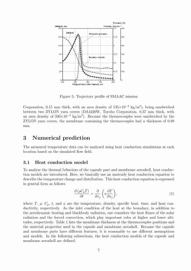
Figure 5: Trajectory profile of SMAAC mission

Corporation, 0.15 mm thick, with an area density of 135×10−3 kg/m2), being sandwichedbetween two ZYLON yarn covers (DA4220W, Toyobo Corporation, 0.37 mm thick, withan area density of 330×10−3 kg/m2). Because the thermocouples were sandwiched by theZYLON yarn covers, the membrane containing the thermocouples had a thickness of 0.89mm.

3 Numerical prediction

The measured temperature data can be analyzed using heat conduction simulations at eachlocation based on the simulated flow field.

3.1 Heat conduction model

To analyze the thermal behaviors of the capsule part and membrane aeroshell, heat conduc-tion models are introduced. Here, we basically use an unsteady heat conduction equation todescribe the temperature change and distribution. This heat conduction equation is expressedin general form as follows:

∂ (ρCpT )

∂t=

∂

∂xj

(κ∂T

∂xj

), (1)

where T , ρ, Cp, t, and κ are the temperature, density, specific heat, time, and heat con-ductivity, respectively. As the inlet condition of the heat at the boundary, in addition tothe aerodynamic heating and blackbody radiation, one considers the heat fluxes of the solarradiation and the forced convection, which play important roles at higher and lower alti-tudes, respectively. Table 1 lists the membrane thickness at the thermocouples positions andthe material properties used in the capsule and membrane aeroshell. Because the capsuleand membrane parts have different features, it is reasonable to use different assumptionsand models. In the following subsections, the heat conduction models of the capsule andmembrane aeroshell are defined.

7

TC7

TC8

TC5

TC6TC3

ZYLON yarn cover

Thermocouples

Capsule

Lamellas

Figure 6: Thermocouples.

Table 1: Material properties of capsule part and membrane aeroshell.

Cepla Aluminum Brass ZYLONThickness at thermocouples (l), mm - - - 0.89

Density (ρ), kg/m3 1400 2700 8560 900Specific heat (Cp), J/kg.K 1050 900 385 1000

Heat conductivity (κ), W/m·K 0.290 237 106 0.2Emissivity (ε) 0.9 0.3 0.1 0.9

8

3.1.1 Capsule part

Because the capsule part has basically an axisymmetric configuration, the two-dimensionalaxisymmetric form of Eq. (1) is used. At the inlet boundary, the heat flux on the vehiclesurface is given by

Q =

{qconv − εσ (T 4 − T 4

b ) + asolarIsolar, during aerodynamic heating;−εσ (T 4 − T 4

b ) + asolarIsolar − h (T − Tatm) , otherwise.(2)

where qconv is the convective heat flux on the capsule surface by aerodynamic heating; andε, σ, Isolar, h, and Tatm are the emissivity, Stefan-Boltzmann constant, solar constant, heattransfer coefficient, and atmospheric temperature, respectively. The SMAAC flies at certainangle to the solar rays, and there is reflection on the membrane surface. Thus, the coefficient(asolar) is multiplied to evaluate the net solar radiation. In the calculation, asolar is simply setto 0.25. The forced convection term appears at altitude, except for the aerodynamic heatingduration. The heat transfer coefficient is given by

h =Nuκatm

L, (3)

Nu = 2 + (0.4Re1/2 + 0.06Re2/3)Pr0.4(µ

µs

)1/4. (4)

where Nu, κatm, and L are respectively the Nusselt number, heat conductivity of air, andcharacteristic length of SMAAC; and Re, Pr, and µs are the Reynolds number, Prandtlnumber, and viscosity at the capsule surface, respectively. The background temperature (Tb)is given based on Ref [22].

Figure 7(a) shows the computational grid system for the heat conduction model of thecapsule. The heat conduction equation in the capsule part is solved using a multi-blockmethod. At each block interface, information about the properties between two blocks isexchanged at each time step. Figure 7(b) shows the computational domain and boundaryconditions. At the inlet, the heat fluxes based on the aerodynamic heating, blackbody radia-tion, solar radiation, and forced convection are given. An axisymmetric condition is imposedalong the center axis. Adiabatic conditions are imposed at the backsides of the antenna coverand aluminum capsule. An initial temperature of 295 K is given based on the measured datawhen being separated from the sounding rocket.

3.1.2 Membrane part

No temperature gradient in the thickness direction is assumed because the membrane isrelatively thin. Thus, the membrane temperature predicted herein is an averaged value inthe thickness direction. The zero-dimensional form in the spatial direction of Eq. (1) is used.

∂ (ρCpT )

∂t= Q. (5)

Blackbody radiations on the front and back sides of the membrane are considered. Thebackground temperatures Tb are the same at the two sides. At the inlet boundary, the heatflux on the membrane surface is slightly different from that of the capsule part, which is givenby

Q =

{qconv − 2εσ (T 4 − T 4

b ) + asolarIsolar, during aerodynamic heating;−2εσ (T 4 − T 4

b ) + asolarIsolar − 2h (T − Tatm) , otherwise.(6)

9

x, mm

y, m

m

0 20 40 60 80 1000

20

40

60

80

100

Antenna cover (Cepla: Block1) Capsule

(Aluminum: Block2)

Capsule (Aluminum: Block3)

Antenna plate(Brass: Block4)

(a) Computational grid system.

x, mm

y, m

m

0 20 40 60 80 1000

20

40

60

80

100Inlet (Aerodynamic heating, radiation..)

Adiabatic

Axisymmetric

Measuring point

(b) Computational domain and boundary conditions.

Figure 7: Computational conditions of heat conduction model for capsule part

The model parameters of Eq. (6) are the same as those of Eq. (2), except for the Nusseltnumber, which is evaluated by the following expression:

Nu =

{0.664Re1/2Pr1/3, if Re < 105;

0.037Re4/5Pr1/3, if Re ≥ 105.(7)

Note that the time scale (t = ρCp/κ) of the heat conduction of the membrane in the thicknessdirection is approximately 3.6 s from Table 1.

3.2 Flow field model

Unlike the flow field simulation for a conventional reentry vehicle, it is important to considerthe deformation of the inflatable aeroshell in the flow field simulation for the inflatable reentryvehicle.

3.2.1 Governing equations

In this paper, the following assumptions are employed. (1) The flow is laminar or turbulent,steady, continuum, and axisymmetric. (2) The inflow gas is air. (3) No chemical reactionoccurs. (4) The translation, rotation, and vibration modes of internal energy freedom areconsidered, while each temperature is equilibrated.

The flow field is described by the Navier-Stokes equations and the equation of state. Theconsidered gases are molecular nitrogen and oxygen (ns = nm = 2). The Navier-Stokesequations are composed of the total mass, momentum, and total energy conservations, which

10

can be expressed as follows:

∂ρ

∂t+

∂

∂xj

(ρuj) = 0, (8)

∂ (ρuj)

∂t+

∂

∂xj

(ρuiuj + δijp) =∂τij∂xj

, (9)

∂E

∂t+

∂

∂xj

[(E + p)uj] =∂

∂xj

(ujτij) +∂qj∂xj

, (10)

where δij is the Kronecker delta. Furthermore, τij and qj are the stress tensor and heat flux,which are, respectively, given by

τij = (µ+ µt)

(∂ui

∂xj

+∂uj

∂xi

− 2

3

∂uk

∂xk

δij

)− 2

3ρkδij, (11)

qj = (λ+ λt)∂T

∂xj

. (12)

The equation of state can be expressed as

p =ns∑s=1

ρsRsT = ρRT. (13)

The total energy E is given by

E =ns∑s=1

5

2ρsRsT +

nm∑s=1

ρsRsΘvib,s

exp (Θvib,s/T )+

1

2ρujuj + ρk, (14)

where Θvib,s is the vibrational characteristic temperature. Transport properties, such asviscosity and thermal conductivity, are evaluated by Yos’ formula [23], which is based on thefirst Chapman-Enskog approximation. The collision cross sections are given by Gupta [24].As a turbulence model, the shear stress transport (SST) turbulence model [25] is adopted.The turbulent kinetic energy k and the turbulent viscosity µt in Eq. (11) can be obtainedwith the SST turbulence model. The turbulent heat conductivity λt in Eq. (12) is evaluatedusing the turbulent Prandtl number Prt and the specific heat at constant pressure Cp asλt = Cpµt/Prt. In the present study, Prt was set to 0.9.

The governing equations are transformed for a generalized coordinate system and aresolved using a finite volume approach. All the flow properties are set at the center of acontrol volume. The inviscid fluxes in the flow-field equations are evaluated using the SLAUscheme [26], and all the viscous terms are calculated using the second-order central differencemethod. The spatial accuracy is thus essentially second order. Time integration is performedusing an implicit time-marching method. The governing equation system is transformed intothe delta form, and the solution is updated at each time step. We employ the lower-uppersymmetric Gauss-Seidel (LU-SGS) method [27].

3.2.2 Boundary and calculation conditions

At the inflow, the freestream parameters are given following the orbit data [18]. As outflowconditions, all the flow properties are determined by the zeroth extrapolation, because theflow was supersonic in most regions. The non-slip condition for the velocity is imposed at

11

Table 2: Calculation conditions.

Elapsed time, s 301 304 308 312 316 324 328 332

Altitude, km 94.0 90.1 86.0 82.0 77.0 68.1 63.0 58.9Velocity, m/s 1159.3 1191.0 1220.8 1251.6 1284.5 1324.5 1315.9 1249.5Density, kg/m3 1.70E-6 3.48E-6 6.95E-6 1.34E-5 3.03E-5 1.12E-4 2.25E-4 4.24E-4Temperature, K 179.2 188.1 192.3 197.7 203.7 221.5 235.2 248.3

336 340 341 344 349 351 356

54.0 50.0 49.0 47.0 44.0 43.0 41.01127.6 930.0 871.3 749.7 552.4 485.7 364.86.95E-4 1.13E-3 1.30E-3 1.67E-3 2.46E-3 2.84E-3 3.74E-3257.3 263.6 263.3 263.0 260.6 258.6 254.6

the surfaces, and no pressure gradient normal to the wall is assumed. The temperature isfixed at 300 K at the surface. An axisymmetric condition is imposed along the center axis.

The present calculations are performed for 15 cases at altitudes ranging from 94.0 km(t = 300 s) to 41.0 km (t = 356 s), as listed in Table 2. The inflow parameters such as thefreestream velocity, density, and temperature are given according to these flight conditions.The computational grid system of the initial state at an altitude of 58.9 km is shown in Fig.8, although different grid systems are used for each altitude.

3.2.3 Membrane deformation

A membrane aeroshell generally deforms due to the aerodynamic force during atmosphericflight [28]. In the present paper, this membrane deformation is expressed using a particle-based model. It is assumed that the membrane consists of virtual particles, with springsconnecting the particles. The virtual particle position (r) can be described using the followingequation of motion:

ρh0S0d2r

dt2= FE + FA, (15)

where the (j + 1/2)th components of the elastic force FE and aerodynamic force FA arerespectively given by

FE,j+1/2 = Ehj+1/2lj+1/2

εj(j+1/2) + νεk(j+1/2)

1− ν2, (16)

FA,j+1/2 = pj+1/2Sj+1/2. (17)

Strains ε are expressed with length lj and initial length lj0 between virtual particles as

εj(j+1/2) =lj(j+1/2) − lj0(j+1/2)

lj0(j+1/2)

,

εk(j+1/2) =lk(j+1/2) − lk0(j+1/2)

lj0(j+1/2)

,

The Young’s modulus E and Poisson’s ratio ν of the ZYLON were set to 30 MPa and 0.3,respectively. These parameters are tuned so that the stretch of the aeroshell because of the

12

x, mm

y, m

m

-200 0 200 4000

200

400

600

800

1000

1200

Figure 8: Computational grid system at an altitude of 58.9 km.

membrane deformation corresponds to the flight experimental results which were constructedbased on the images taken by onboard JPEG cameras mounted on the backside of the SMAAC[18]. Thus, the textile properties of the aeroshell are assumed to be isotropic. The densityis the same as that listed in Table 1. Parameter CAE, which represents the ratio of theaerodynamic force to the elastic force of the membrane, is defined by

CAE =ρ∞U2

∞L

Eh0

, (18)

where the thickness of the ZYLON fabric h0 is 0.155 mm. Thus, the CAE value of the SMAACis on the order of 10−1 during aerodynamic heating.

The equation of motion is solved using the 4th order Runge-Kutta method. As theboundary, the displacement is fixed on the capsule-side end. The free-end condition on theside of the torus is set in the x direction, and the fixed-end condition is set in the y direction.The flow field is simulated coupled with the membrane deformation.

4 Results and Discussion

4.1 Validation of heat conduction model

The temperature history measured by the TC1 thermocouples on the membrane aeroshellduring the SMAAC atmospheric reentry is shown in Fig. 9. The histories measured by sixother thermocouples (TC2, TC3, and TC5-TC8) show tendencies similar to that by TC1, and

13

Elapsed time after launch, sec

Tem

pera

ture

, K

200 400 600 800 1000 1200200

250

300

350

400

Temperature (Flight, CH1)Temperature (CFD)Atmospheric temperature

Figure 9: Histories of measured and predicted temperatures without aerodynamic heatingand atmospheric temperature.

these profiles are shown in the appendix. This figure includes the atmospheric temperatureand temperature profile calculated by the heat conduction model on the membrane of theSMAAC without aerodynamic heating (qconv = 0), to validate the model factors (i.e., thesolar radiation coefficient “asolar” and heat transfer coefficient “h”) in the heat conductionmodel. Based on this history, the elapsed time after launch at which the temperature at themembrane reaches its peak value is about 350 s, and its peak temperature is about 380 K.

We estimate that aerodynamic heating occurs from t = 300 to t = 350 s. At higheraltitudes, the membrane is cooled by blackbody radiation. After aerodynamic heating, themeasured temperature rapidly decreases due to this blackbody radiation, in addition to theforced convection. On the other hand, the membranes are only equilibrated with the atmo-spheric temperature by the forced convection at lower altitudes. The predicted temperatureshows good agreement with the measured temperature, except for the aerodynamic heat du-ration. This indicates that the parameters of the heat conduction model adequately describethe experimental environment. In the present paper, the convective heat flux by aerodynamicheating is calculated using the computational fluid dynamics (CFD).

4.2 Aerodynamic heating prediction

Numerical simulations of the flow fields during aerodynamic heating were performed for the15 altitudes listed in Table 2. The Reynolds number of the flow field ranges from 104 to 105

when strong aerodynamic heating occurs. Thus, the flow field is expected to transition froma laminar to turbulent flow during reentry. In the present study, simulations of the laminarand turbulent cases were performed, and their results are compared with the measured tem-perature histories. The heat flux profiles predicted by the CFD technique are shown in thissection.

Figures 10(a), 10(b), 10(c), and 10(d) show the temperature distributions with streamtraces for the laminar and turbulent (SST model) cases without/with the membrane defor-mation model at an altitude of 58.9 km. It is confirmed that a shock wave is formed in

14

front of the vehicle, where the temperature becomes uniformly constant from the capsuleto the torus. In addition, Figs. 11(a) and 11(b) show comparisons of the heat flux profilesalong the SMAAC surface between the laminar and turbulent cases at an altitude of 58.9 kmwithout/with the membrane deformation model, respectively.

The membrane is largely deformed by the aerodynamic force when considering the mem-brane deformation model. In contrast with a rigid vehicle such as a conventional reentrycapsule, the membrane aeroshell of an inflatable vehicle such as the SMAAC can be deformedduring flight. It is expected that the deformation model used in the numerical simulation canhave an influence on the prediction of the heat flux on the membrane surface. The heat fluxon the membrane surface with the deformation model becomes low compared with the rigidmodel. On the other hand, the heat flux on the capsule with the deformation model onlychanges slightly. This is mainly because the shock stand-off distance near the stagnation lineshortens. These features are attributed to the shock layer formation, with the deformationeffect that the inflatable torus moves backward because of the stretching of the aeroshell,with a reduction in the effective flare angle. Thus, it is necessary to introduce a membranedeformation model when predicting the aerodynamic heating for this kind of vehicle. In thefollowing discussions, the heat flux predicted with the membrane deformation model is used.

For the case of laminar flow, the flow in the shock layer separates on the capsule surface,and a large recirculation region appears along the overall membrane aeroshell. On the otherhand, no recirculation region appears for the case of turbulent flow. This is because theturbulent viscosity (eddy viscosity) in the shock layer becomes high considering the turbulencemodel. This is expected to increase the heat flux on the capsule and membrane surfaces,because the temperature gradient in the spatial direction near the SMAAC surface becomeshigh. The heat flux at the top of the capsule become about 16.5 kW/m2 for the turbulentflow case, because turbulence develops near the capsule. Note that the numerical solution ofthe laminar flow is smaller than the heat flux based on the empirical model that has beenused for the design of the SMAAC. For the case of laminar flow, there is high heat flux on ajoint part between the membrane aeroshell and inflatable torus positions at the reattachmentpoint of the recirculation region. However, in most regions of the membrane, the heat fluxremains relatively low, because the high-temperature gas in the shock layer hardly inflowsto the recirculation region. On the other hand, for the case of turbulent flow, the heat fluxdistribution on the membrane from the capsule side to the torus side is almost constant.As confirmed in the heat flux profile for the laminar flow, an obvious reattachment point isnot seen for the turbulence flow case. The strong diffusivity of the turbulence causes high-temperature gas to flow into the recirculation region. As a result, the heat flux profile alongthe membrane surface considering the turbulence model becomes smooth.

A predictive tool of aerodynamic heating and the thermal environment around the in-flatable vehicle was reconstructed for suborbital reentry. However, for orbital speed reentry(more than 7 km/s) from a low Earth orbit, further development of the predictive tool isrequired. Because the Mach number in orbital reentry becomes higher than that of the sub-orbital reentry, real gas effects, e.g., chemical reactions, excitation of internal energy, andenergy transfer, can occur at certain altitudes. These effects are neglected in the predictivetool of aerodynamic heating. However, the present tool can be effective for thermal environ-ment prediction at higher and lower altitudes before and after aerodynamic heating. Themembrane aeroshell and inflatable torus are anisotropic, and the isotropic analysis conductedis generally insufficient, as reported in Ref. [9]. Although an isotropic analysis can be effectiveat an initial stage of design, introduction of an orthotropic analysis may be needed for theaccurate prediction of membrane deformation.

15

(a) Laminar case without deformation model. (b) Turbulent case without deformation model.

(c) Laminar case with deformation model. (d) Turbulent case with deformation model.

Figure 10: Distributions of temperature and stream traces around SMAAC at altitude of58.9 km.

16

y, mm

Hea

t flu

x, W

/m2

0 100 200 300 400 500 6000

2500

5000

7500

10000

12500

15000

17500

CHF(Laminar)CHF(Turbulent-SST)

(a) Without membrane deformation model

y, mm

Hea

t flu

x, W

/m2

0 100 200 300 400 500 6000

2500

5000

7500

10000

12500

15000

17500

CHF(Laminar)CHF(Turbulent-SST)

(b) With membrane deformation model

Figure 11: Comparison of radial profiles of convective heat fluxes on SMAAC surface betweenlaminar and turbulent cases at altitude of 58.9 km.

4.3 Thermal behavior of capsule

The heat conductions in the capsule part are investigated using the experimental data andsimulation results with the deformation for the laminar and turbulent cases. Figures 12(a)and 12(b) show comparisons of these at the backside of the semi-spherical shell of the alu-minum capsule. Measured temperature increases of approximately 20 K are observed. Thetemperature reaches the maximum value of 315 K for the aluminum capsule. The increasesin temperature are due to aerodynamic heating during the elapsed time period of 350 s to400 s. Then, the capsule is cooled by the atmosphere.

For the aluminum capsule, the predicted temperatures for the case of laminar flow showgood agreement with the measured temperatures. On the other hand, for the case of tur-bulence, the predicted temperatures tend to overestimate the measured temperatures. It ispossible that the distance travelled by the flow on the capsule surface is too short to tran-sition to turbulence. Thus, if the flow near the capsule is laminar, a reasonable agreementis obtained. In this case, the maximum heat flux at the stagnation point is expected to beabout 14 kW/m2 during the reentry flight.

4.4 Thermal behavior of membrane

Figure 13 show comparisons of the measured and predicted temperatures at thermocouplespositions TC1, TC2, and TC5. This figure includes the heat flux histories predicted bythe CFD with the deformation model. Similar to the capsule, the membrane is heated byaerodynamic heating. These temperature profiles are similar to the profiles at the otherthermocouples, which are shown in the appendix. The maximum temperature is 380 K atan elapsed time of approximately 350 s. Compared with the measured temperatures, theelapsed times needed to reach the peak temperatures with the numerical method are short.As mentioned above, the time scale for the heat conduction of the membrane is approximately3-4 s. This is mainly due to neglecting the temperature gradient in the spatial direction in theheat conduction model. The temperature histories measured with thermocouples TC1, TC2,

17


Tem

pera

ture

, K

Hea

t fl

ux, W

/m2

250 300 350 400 450 500 550 600290

300

310

320

330

0

5000

10000

15000

20000Temperature (Aluminum, Flight)Temperature (Aluminum, Simulation)Heat flux (Simulation)

(a) Laminar case.


Tem

pera

ture

, K

Hea

t fl

ux, W

/m2

250 300 350 400 450 500 550 600290

300

310

320

330

0

5000

10000

15000

20000Temperature (Aluminum, Flight)Temperature (Aluminum, Simulation)Heat flux (Simulation)

(b) Turbulent case.

Figure 12: Histories of measured and predicted temperatures and heat fluxes at backside ofsemi-spherical shell of aluminum capsule.

and TC5 are very similar to each other. The phases of the three thermocouples positionsare respectively different, as shown in Fig. 2, while the radii of the mounting positions areclose (TC1: y = 254 mm, TC2: y = 273 mm, and TC5: y = 254 mm). It was reported byNagata et al. [20] that the SMAAC vehicle flew at the angle of attack during aerodynamicheating. On the other hand, the vehicle had an angular velocity around the symmetricalbody axis. It was reasonable to use a time-averaged heat flux on the membrane surface inthe circumferential direction, and the temperature profiles became almost constant in thisdirection.

Comparisons of the measured and predicted temperature distributions in the radial di-rection on the membrane for elapsed times of 300, 348, and 380 s at each thermocouples areshown in Fig. 14. A feature of the measured temperature distribution is an almost constantprofile for each thermocouples. Because the membrane is thin, its heat conduction in theradial direction is never dominant compared with that in the thickness direction. This meansthat the heat flux profile along the membrane surface for the flight is also constant duringthe aerodynamic heating. Compared with the measured temperature, for the laminar flowcalculation, the predicted temperatures at the thermocouples near the capsule side (e.g., TC3and TC6) become low due to the presence of the recirculation region. On the other hand,for the case of the turbulent flow in the prediction, no recirculation region appears, and theheat flux shows a uniform distribution on the membrane. It is suggested that the heat fluxesat each point where the thermocouples are mounted are in the same range, as indicated bythe measured temperature profiles shown in Fig. 14. The temperatures predicted with theturbulent model show qualitatively good agreement with the measured temperatures. Hence,it is reasonable to conclude that there is no recirculation region in the shock layer, and theflow field near the membrane surface is turbulent during aerodynamic heating in the flight.

A feature of the aerodynamic heating around the SMAAC is that the heat flux profiles arealmost constant in the circumferential and radial directions. This is thought to be becausethe flow field is temporally averaged by the angular velocity and is turbulent. In addition, acomparison of the measured and predicted temperature histories suggests that the peak heat

18


Tem

pera

ture

, K

Hea

t fl

ux, W

/m2

250 300 350 400 450 500 550 600200

250

300

350

400

450

0

1500

3000

4500

6000

7500Temperature (Flight, CH1)Temperature (Flight, CH2)Temperature (Flight, CH5)Temperature (Simulation)Heat flux (Simulation)

(a) Laminar case


Tem

pera

ture

, K

Hea

t fl

ux, W

/m2

250 300 350 400 450 500 550 600200

250

300

350

400

450

0

1500

3000

4500

6000

7500Temperature (Flight, CH1)Temperature (Flight, CH2)Temperature (Flight, CH5)Temperature (Simulation)Heat flux (Simulation)

(b) Turbulent case

Figure 13: Histories of measured and predicted temperatures and heat fluxes at TC1, TC2,and TC5 positions.

y, mm

Tem

pera

ture

, K

100 150 200 250 300 350 400 450200

250

300

350

400

450 Flight (t=316 s)Flight (t=348 s)Flight (t=380 s)Simulation (t=316 s)Simulation (t=348 s)Simulation (t=380 s)

(a) Laminar case

y, mm

Tem

pera

ture

, K

100 150 200 250 300 350 400 450200

250

300

350

400

450 Flight (t=316 s)Flight (t=348 s)Flight (t=380 s)Simulation (t=316 s)Simulation (t=348 s)Simulation (t=380 s)

(b) Turbulent case

Figure 14: Comparison of measured and predicted temperature distributions on membrane.

19

flux on the membrane is more than 5 kW/m2.

5 Conclusions

A suborbital reentry demonstration of an inflatable vehicle using a sounding rocket was suc-cessfully performed. The temperature histories were measured using seven thermocouplesembedded on the backside of a membrane aeroshell. In addition, the temperature profileat the backside of the semi-spherical shell of the aluminum capsule was obtained using atemperature transducer. To investigate the aerodynamic heating behavior around the in-flatable vehicle during atmospheric reentry, the measured temperatures were compared withthe temperatures obtained using an unsteady heat conduction equation. The heat fluxesby aerodynamic heating that were used as the input parameters of the heat conductionmodel were predicted for cases of laminar and turbulent flows with the simulation modelusing computational fluid dynamics. Using the reentry trajectory reconstructed based onthe measured data and an atmospheric model, flow-field simulations were performed for 15cases, including a freestream condition for an altitude. On the membrane aeroshell, thepredicted temperature histories for the case of turbulent flow showed good agreement withthe measured temperatures, while those for the laminar flow were generally underestimatedbecause of the recirculation region and lower heat flux. On the other hand, the predictedtemperature on the capsule for the case of laminar flow showed good agreement with theexperimental data. It was suggested that the flow field near the capsule surface was possiblylaminar, and then transitioned into turbulence on the membrane during aerodynamic heat-ing. These results suggested that an aerodynamic heating reduction was demonstrated bythe low-ballistic-coefficient flight of the thin-membrane inflatable vehicle.

Appendix

Comparisons of measured and predicted temperatures at positions of thermocouples TC3,TC6, TC7, and TC8 are shown in Figs. 15, 16, 17, and 18, respectively.

Acknowledgments

The sounding rocket experiment was carried out at the Uchinoura Space Center (USC) incollaboration with the Research and Operation Office for Sounding Rocket (ROOSR) atthe Japan Aerospace Exploration Agency. This research activity was also supported by theSteering Committees for Space Engineering (SCSE). We would like to thank the members ofROOSR, USC, and SCSE for their useful advice and support.

The computation was mainly carried out using the computer facilities at the ResearchInstitute for Information Technology, Kyushu University.

References

[1] M. Graβilin and U. Schottle. “Flight Performance Evaluation of the Reentry MissionIRDT-1”. In Papers Presented at the 52nd International Astronautical Congress, IAFPaper 01-V305, Toulouse, France, October 1 - 5 2001.

20

[2] S.J. Hughes, R.A. Dillman, B.R. Starr, R.A. Stephan, M.C. Lindell, C.J. Player, andD.F.M. Cheatwood. “Inflatable Re-entry Vehicle Experiment (IRVE) Design Overview”.AIAA Paper 2005-1636, 2005.

[3] R.R. Rohrschneider and R.D. Braun. “A Survey of Ballute Technology for Aerocapture”.Journal of Spacecraft and Rockets, 44(1):10–23, January - February 2007.

[4] P. Reynier and D. Evans. “Postflight Analysis of Inflatable Reentry and Descent Technol-ogy Blackout During Earth Reentry”. Journal of Spacecraft and Rockets, 46(4):800–809,July-August 2009.

[5] S.J. Hughes, D.F.M. Cheatwood, A.M. Calomino, and H.S. Wright. “Hypersonic In-flatable Aerodynamic Decelerator (HIAD) Technology Development Overview”. AIAAPaper 2011-2524, 2011.

[6] T. Abe. “A Self-Consistent Tension Shell Structure for Application to AerobrakingVehicle and Its Aerodynamic Characteristics”. AIAA Paper 1988-3405, 1988.

[7] I.G. Clark, A.L. Hutchings, C.L. Tanner, and R.D. Braun. “Supersonic Inflatable Aero-dynamic Decelerators for Use on Future Robotic Missions to Mars”. Journal of Spacecraftand Rockets, 46(2):340–352, March - April 2009.

[8] I.G. Clark. Aerodynamic Design, Analysis, and Validation of a Supersonic InflatableDecelerator. PhD thesis, Georgia Institude of Technology, july 2009.

[9] C.L. Tanner. Aeroelastic Analysis and Testing of Supersonic Inflatable AerodynamicDecelerators. PhD thesis, Georgia Institude of Technology, May 2012.

[10] K. Yamada, D. Akita, E. Sato, K. Suzuki, T. Narumi, and T. Abe. “Flare-Type Mem-brane Aeroshell Flight Test at Free Drop from a Balloon”. Journal of Spacecraft andRockets, 46(3):606–614, May-June 2009.

[11] K. Yamada, T. Abe, K. Suzuki, N. Honma, M. Koyama, Y. Nagata, D. Abe, Y. Kimura,A.K. Hayashi, D. Akita, and H. Makino. “Deployment and Flight Test of InflatableMembrane Aeroshell using Large Scientific Balloon”. AIAA Paper 2011-2579, 2011.

[12] K. Yamada, M. Koyama, Y. Kimura, K. Suzuki, T. Abe, and A.K. Hayashi. “Hyper-sonic Wind Tunnel Test of a Flare-type Membrane Aeroshell for Atmospheric EntryCapsule”. ISTS Special Issue: Selected papers from the 27th ISTS, Transactions ofJSASS, 7(ists27):27–32, 2010.

[13] K. Yamada, T. Sonoda, K. Nakashino, and T. Abe. “Structural Strength of Flare-typeMembrane Aeroshell Supported by Inflatable Tours against Aerodynamic Force”. InProceedings of 28th International Symposium on Space Technology and Science, ISTS2011-c-34, Okinawa, Japan, June 5 - 12 2011.

[14] Y. Takahashi, K. Yamada, and T. Abe. “Radio Frequency Blackout Possibility for anInflatable Reentry Vehicle”. AIAA Paper 2012-3110, 2012.

[15] Y. Takahashi, K. Yamada, and T. Abe. “Examination of Radio Frequency Blackout foran Inflatable Vehicle during Atmospheric Reentry”. Journal of Spacecraft and Rockets,51(2):430–441, March 2014.

21

[16] K. Yamada, T. Abe, K. Suzuki, O. Imamura, and D. Akita. “Reentry DemonstrationPlan of Flare-type Membrane Aeroshell for Atmospheric Entry Vehicle using a SoundingRocket”. AIAA Paper 2011-2521, 2011.

[17] K. Yamada, Y. Nagata, T. Abe, K. Suzuki, O. Imamura, and D. Akita. “Subor-bital Reentry Demonstration of Inflatable Flare-Type Thin-Membrane Aeroshell Usinga Sounding Rocket”. Journal of Spacecraft and Rockets, 52(1):275–284, February-March2015.

[18] K. Yamada, Y. Nagata, T. Abe, K. Suzuki, O. Imamura, and D. Akita. “ReentryDemonstration of Flare-type Membrane Aeroshell for Atmospheric Entry Vehicle usinga Sounding Rocket”. AIAA Paper 2013-1388, 2013.

[19] K. Yamada, Y. Nagata, N. Honma, D. Akita, O. Imamura, T. Abe, and K. Suzuki.“Reentry Demonstration Deployable and Flexible Aeroshell for Atmospheric-Entry Vehi-cle using Sounding Rocket”. In Proceedings of 63th International Astronautical Congress,AC-12-D2.3.3, Naples, Italy, October 1 - 5 2012.

[20] Y. Nagata, K. Yamada, T. Abe, and k Suzuki. “Attitude Dynamics for Flare-typeMembrane Aeroshell Capsule in Reentry Flight Experiment”. AIAA Paper 2013-1285,2013.

[21] C.G. Justus and D.L. Johnson. “NASA/MSFC Global Reference Atmospheric Model―1999 Version (GRAM-99)”. NASA TM-1999-209630, May 1999.

[22] L.A. Carlson and W.J. Horn. “New Thermal and Trajectory Model for High-AltitudeBalloons”. Journal of Aircraft, 20(6):500–507, June 1983.

[23] J.M. Yos. “Transport Properties of Nitrogen, Hydrogen Oxygen and Air to 30,000 K”.TRAD-TM-63-7, Research and Advanced Development Division, AVCO Corp., 1963.

[24] R.N. Gupta, J.M. Yos, R.A. Thompson, and K.P. Lee. “A Review of Reaction Ratesand Thermodynamic and Transport Properties for an 11-Species Air Model for Chemicaland Thermal Nonequilibrium Calculations to 30000 K”. NASA RP-1232, Aug. 1990.

[25] F.R. Menter. “Two-Equation Eddy-Viscosity Turbulence Models for Engineering Appli-cations”. AIAA Journal, 32(8):1598–1605, August 1994.

[26] E. Shima and K. Kitamura. “Parameter-Free Simple Low-Dissipation AUSM-FamilyScheme for All Speeds”. AIAA Journal, 49(8):1693–1709, August 2011.

[27] A. Jameson and S. Yoon. “Lower-Upper Implicit Schemes with Multiple Grids for theEuler Equations”. AIAA Journal, 25(7):929–935, July 1987.

[28] K. Yamada, Y. Kato, and T. Abe. “Numerical Simulation of Hypersonic Flow aroundFlare-Type Aeroshell with Torus Frame”. In Proceedings of 6th Asia Workshop on Com-putational Fluid Dynamics, Kashiwa, Japan, March 16 2009.

22


Tem

pera

ture

, K

Hea

t fl

ux, W

/m2

250 300 350 400 450 500 550 600200

250

300

350

400

450

0

1500

3000

4500

6000

7500Temperature (Flight, CH3)Temperature (Simulation)Heat flux (Simulation)

(a) Laminar case

Elapsed time after launch, secT

empe

ratu

re, K

Hea

t fl

ux, W

/m2

250 300 350 400 450 500 550 600200

250

300

350

400

450

0

1500

3000

4500

6000


(b) Turbulent case

Figure 15: Histories of measured and predicted temperatures and heat fluxes at TC3 position(y = 141 mm).


Tem

pera

ture

, K

Hea

t fl

ux, W

/m2

250 300 350 400 450 500 550 600200

250

300

350

400

450

0

1500

3000

4500

6000


(a) Laminar case


Tem

pera

ture

, K

Hea

t fl

ux, W

/m2

250 300 350 400 450 500 550 600200

250

300

350

400

450

0

1500

3000

4500

6000


(b) Turbulent case


23


Tem

pera

ture

, K

Hea

t fl

ux, W

/m2

250 300 350 400 450 500 550 600200

250

300

350

400

450

0

1500

3000

4500

6000


(a) Laminar case

Elapsed time after launch, secT

empe

ratu

re, K

Hea

t fl

ux, W

/m2

250 300 350 400 450 500 550 600200

250

300

350

400

450

0

1500

3000

4500

6000


(b) Turbulent case



Tem

pera

ture

, K

Hea

t fl

ux, W

/m2

250 300 350 400 450 500 550 600200

250

300

350

400

450

0

1000

2000

3000

4000

5000

6000


(a) Laminar case


Tem

pera

ture

, K

Hea

t fl

ux, W

/m2

250 300 350 400 450 500 550 600200

250

300

350

400

450

0

1500

3000

4500

6000


(b) Turbulent case


24

aerodynamic heating around flare-type membrane … · instructions for use title aerodynamic...

Documents