aerodynamic heating effects on a flying object at

8/3/2019 Aerodynamic Heating Effects on a Flying Object At

http://slidepdf.com/reader/full/aerodynamic-heating-effects-on-a-flying-object-at 1/5

Aerodynamic Heating Effects on a Flying Object at

SI414

High Speeds

Difkrenr poinrs in and on he exlemd store

D. ren GUNDUZ, Alper l&VER. Fato$Esen ORI-IAN, Dr. Mehmer Al i AK

TOBITAK Defence Industry Research and Development Institude

TUBITAK SAGE, Pk:16 06261 Mamak Ankara, torhan~saee.tubitaksov.tr:Turkey

Abstract- In a research project held by ToEtTAK SAGE,temperature, pressure, and acceleration values were measuredon an external store curried under n wing of an aircrafi a t

various flight proliles. To choose the right sensors and devicesfor such night tests, it's important to know the temperaturelimits that al l the devices might be exposed to. This io because

each sensor has optimal performance in some tight temperaturelevels, and dors not function at at1 when it s temperature limitsare exceeded.

Flight speeds and altitudes of the llight profiles were wet1defined before the tests. When the sea level temperature is

laown, corresponding temperature values of different altitudescan be calculated easily. Literature surveys show that thedominant factor affecting the outer surfac e tempe rature of

flying objects at high speeds is not the ambient air temperaturebut the aerodynam ic heating enect.

There are a few equations availablr. in the literature to

calculate the aerodynamic healing as a function of the ambientair temperature and t h e night speed. These equations ar epresented in come papers and books, b u t verification of themcouldn't be found. Therefo re how confident they are and the

acsu racy leve1 of the equntions are not clear.Bcfore the flight tests, detaikd heat transfer analysis of the

external store and the devices in it werr done using thementioned equations. The temperature measurements takenduring th e flights were compared with t h e analysis and th e

verification of the equations were done.In this paper, the equations, cnlculations, test data and

comparison of the results were presented. Finatly a conclusionwas made about the accuracy level of the equations given in theliterature.

I . LNTRODUCTION

Storage and operational temperature limits of electronic

parts are very limiting. T he expo sition of some parts to a

temperature below -4O'C an d above +85'C may cause critical

problems. For this reason, determination of maximum an d

minimum temperature intervals of the electronic parts fo r

critical flight conditions and making th e design accordingly

gain importance.

During the long period low altitude flights at high speeds,temperature of extemal boundary o f the body may reach very

high values. Similar to that, for long period high altitude

flights a t low speeds, the temperature may drop to very lowvalues

For certain flight conditions heat transfer analysis were

done in order to determine the change in temperature on theexternal store with the help of 2- D an d 3- D numerical

methods. The radiation. convection, conduction heat transfers

and the aerodynamic heating effects were included in this

modeling.

Some flight tests were done to verify the analysis. In these

tests, it was observed whether the temperature o f the elements

reach th e critical values or not by taking data at the flight test

at low an d high altitudes. Maximum and minimum

temperatures that th e electronic cards. eiemcnts on the cards

and the measurement devices resist to storage an d operation

conditions were known. With the help of this observation,

which part exposes how much temperature change and

whether the limits are exceeded or not were determined.

After th e flight tests, rhe needed data for the verification of

the models and the aerodynamic heating calculations were

obtained successfill y.

11. DEVELOPMENT

A 3-D model of external store was prepared by using a

software which makes solution using finite element method.In order to calculate the natural convection heat transfer, the

ai r inside w a s considered as a solid volume. As a result,

248.987 tetrahedron elements and 44.592 nodes on the model

are obtained.

Names an d positions of the temperature sensors are listed in

TABLE I .TABLE I

TEMPERATURE SENSOR POSI'TIOKS

Name f Ih CPosition of the SensorI-emperature Sensor

0-7R03-8977-81051%20.00a2005 E E E . 277

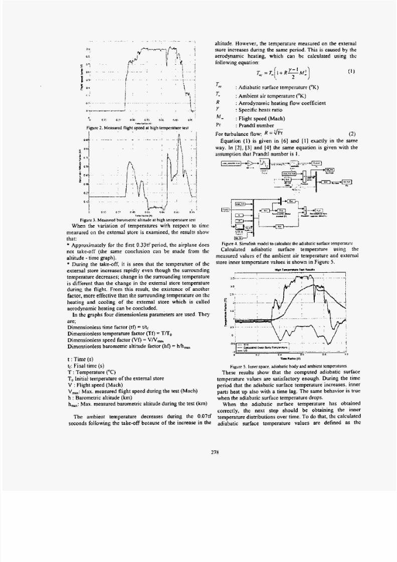
Temperature, velocity and altitude measured during the

high temperature flight tests (low altitude flights at high

speeds) are shown in the Figures 1,2 and 3.

.. . . .S -

-1 0

0 0 - 0 4 0 6 o a 1

ih mm (TII

Figure I . Mcasured iempcraturec 81high temperaturc lest



. . . . . . . . . . . . .. 7 :

altitude. However, the temperature measured on the external

store increases during the same period. Th is is caused by the*.L aerodynamic heating, which can be calculated using the

following equation:

( 1 )

".

2 9.

..........

- o-; ,

f , & _ j : :

i a,

. . . . . . . . . . .j ,; / . i ..:.. y ' - ;

i : Adiabatic surface temprrature ("K)

w, ; T : Ambient air temperature ( O K )

E 0.

o > - . . . . . . ..\ -, R : Aerodynamic heating flow coefficient

: Specific heats ratio

: Flight speed (M ach)

.+ Y

i:

p

"0 c I ai: U &> 65 3 o ct c c, v'9:

Figure 2. Measured flight speed at high temperature test Pr : Prandtt number. n l C t o W

For turbuiance flow; R =f i (21Equation (1 ) is given in 161 and [ t ] exactly i n the same

way. In [2], [3j and 141 the same equation is given with the

. . . . . . . . . . . . . . . . . . . . . . . . . . . . .

assumption that Prandtl number i s I .

*?

. .

..-I -TI <

.....

. & h a ..I L,I. ".U. . . (*, -.:- +=---+J-+..

. I

.

I t

*.,...U,

c 01: 02 7 PI 0 0 0 : 5 % 411. 0 1,

7 b t " F , -rn

"4Figure 3. M m u r e d barumernc ahitud e at high temperature test

When the variation of temperatures with respect to time

measured on th e external store is examined, the results show

that:

* Approximarely for the first 0.33tf period. the +lane does

no t take-off (the same conclusion call be made from the Calculared adiabatic surface temperamre using thealtitude - time graph). measured values of the ambient air temperature and external

* During the take-off, it is seen tha t the temperature o f the Store inner tempe rature values is show n in Figure 5 .

external store increases rapidly even though the surrounding

temperature decreases; change in the surrounding temperature

is different than the ch ange in the extemal store temperatureduring the flight. From this result, the existence of another

factor. more effective than th e surrounding temperature on he

heating and cooling of the external store which is called

aerodynamic heating can be concluded.

In the graphs four dimensionless parameters are used. They

are;Dimensionless time factor (to = tit,

Dimensionless temperature factor (Tf) = T/ToDimensionless speed factor (Vf) = VN , ,

Dimensionless barometric altitude factor (hf) = hh

f : Time (SItl: Final time (s) Figurc 5 . Inner space , adiabatic body and ambient tcmperatuns

T : Temperature ("C) These results show that the computed adiabatic surface

To nitial temperature of the extemal store temperature values are satisfactory enough. During the timeV : FLight speed (Mac h) period that the adiabatic surface temperature increases. innerV Max. measured flight speed during the test (Mach) parts heat up also with a time lag. The same behavior is true

h :Barometric altitude (km) when the ad iabatic surface temperature drops.hmx:Max. measured barom etric altitude during the test (h) When the adiabatic surface temperature has obtained

correctly, the next step should be obtaining the inner

temperature distributions over time. T o do that, the calculated

adiabatic surface temperature values are defined as the

Figure 4. Simulink model to calculate ihe adiabatic surface iempcraturt

HM i rm. w -I

0 G ? 0. Dh C C r n

lima rilslw [If)

Th e ambient temperature decreases during the 0.07tf

seconds foliowing the take-off because of the increase in the



boundary condition of the 3-D computer model. Fmaliy, the

results of the model art shown in Figure 6 .

-1.0 4 5 0 0 5 1 0 1 5 2 0 2 5 30 3 5

Figure 6 Il~mensionless iperamre Idctni variatiun at thc end ofthe totdl

flrght ~ imc nner space IC also included

W ith this method, temperature vanarions of each element

with respect to time can be computed Since there are 24 8 987

eteinents, i t 's impossible to examine each single element

Instead, the elements around the locations where the

measurements were taken during th e tests were compared

with the measurements(Figures 7 , 8 , 9 , 10 and I I)

1 ;

16

1. . .

o. ... L ........... :.. .... __."I. .L_ . .. .JQ: 01 06 a s I D

rt- F L ~ W

Figure 7.Measured an d calculated remperarure factors for S14

- - .

T W F W l q

Figure 8 . Measured and calculated temperature factors for SI

ID

0 0" 0 4 n 6 I t 10

-rimrxtam

F l y r e 9 Mcasured and calculared temperature facloh fnr SY

. . . . . . . . . . . . 1.__. . . . . . . . . . . . . . . . . - lr;.*rnta.--..V"tih! I..

10

0 a: 0 1 W 'I s a 1 l

TIUr.nrm

Figure I I Measured and calculated Iempenturc facton for S2

Another flight test was made to verify the model at the low

temperature limits. Measured ambient temperature, inner

temperature an d calculated outer body temperature plots c m

be seen In the Figure 12 .

27 9



: ?:

= 0 : -::. . . . . . . . . . . . . . . . . ..............

f c y . . .

a ;E -, . . . . . . ! . . . . . . . . . . . . . . . . . . . . . . ..1

1. . . . . . . . ". . . . . . . . . .

: i

~

-2; - 1 . -

. . . . . i . .

e 9 2 n * O F o * L O

7- R r b 10

Figure I? . lnner space,diabalic body and ambient temperatures

This calculated adiabatic surface temperature i s defined as

the boundary condition for the 3-D model. With these

boundary conditions, inner temperamre distribution can be

obtained with a transient (time variant) solution. Since the

model includes too many nodes and elements, one solution

had taken 3-4 days. Therefore, the model was executed only

for the first 0.29tf time period of the flight (Figure 13).

-2.5 -2.0 -1.5 -1.0 -0.5 0 0. 5 l . D 1. 5 2.0

Figure 1 3 . Dimcnsionlrw emperature factor variation at time t-0.29tf (inner

space is also included)

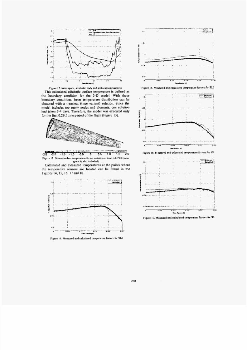
Calculated and measured temperatures at the points where

th e temperature sensors are located can be found in the

Figures 14, 15, 16, I7 and 18.

1 ............ <:--. mu.%, r-I . ' ! ~ ~

. . . . . . . . . . . . . . . . . . . . . . . . . . . . . . . . . . . . . . . . .,& ; .,_ Y S V t d z

i

. . . . . . . .73-

. . . . i . . _I

-__I:-

a 0w. G 119 0 11. Un: a >-!

1n. hneo til]

Figure 15. Measured and calculated temperature factors for SI 2

il-- -4. . . . . . . . . . . . . . -. . 'r_I ! %I;

. . . . . . . . . . . . . .. . 1

O , L . , . . . . . . . . . . . . . . . . . . . . . . . . . . . . .: .................1~ ~ ->

0 0 Vd 0 $10 0 17d 0 :I 0 CJ

T i l r F;.;fm pi)

Figure 16. Measured and calculated temperature factors for SY

. . .. . . . . . . . . . . -_-_ *.- *:u4m,

' __- - k d-.--f

i

~ . . ". . . . . .. .5 -

-: . . . . . . . . . ..: . . . . . . . . . ; . . . . . . . . . . . .E !e .n .

I.................... . . . . ~ . . . . . . . . . . . . . . -

87 5............. . . . . . . . . . ." . . . . . . . . . . . . . . . . . ~. . . .

1. . . ..+ _ ................ . . " .............. .:

0 0F r; ?le. 0 17 1 G3: 0 '.W,

n w r u r w i

Figure 17 . Measured and calculated temperaturefactors for56

Figure 14.Measuredand calcuIated emperalure factors for SI 4

28 0

aerodynamic heating effects on a flying object at

Documents