aerodynamic analysis around a c-class catamaran in...

Aerodynamic Analysis around a C-Class Catamaran in Gust Conditions using LES

and Unsteady RANS Approaches A. Fiumara, Assystem France and ISAE-Supaéro, France, [email protected], [email protected]

N. Gourdain and V.-G. Chapin, ISAE-Supaéro, France, [email protected], [email protected]

J. Senter, Assystem France, France, [email protected]

Abstract: Wingsail is the propulsion mean adopted by the America’s Cup and C-class catamarans. This rig has improved

aerodynamic performance with respect to conventional soft sails enhancing the yacht performance. However due to the higher

forces acting wingsails, the yacht stability can easily be compromised especially in heavy gust wind conditions. The wingsail

response to a gust has been then investigated performing numerical analysis in a C-class catamaran in downwind navigation

conditions. Both a LES and an unsteady RANS approach were used for the simulations. The solutions given by the two

approaches have been compared analyzing both the aerodynamic coefficients and the flow characteristics. The effect of the wind

gust on the wingsail has been further investigated at different gust frequencies. Stall cells appear on the flap surface when the

gust is taking into account affecting the wingsail aerodynamic performance.

NOMENCLATURE

α Angle of attack (°)

δ Flap deflection angle (°)

AW Apparent Wind

AWA Apparent Wind Angle (°)

AWS Apparent Wind Speed (m/s)

BS Boat speed (m/s)

Cµ Momentum coefficient

c Total chord of the wingsail (m)

c1 Main chord (m)

c2 Flap chord (m)

CD Drag coefficient

CF Skin friction coefficient

CL Lift coefficient

Cp Pressure coefficient

F+ Non-dimensional gust frequency

(fgc2/ V∞)

fg Gust frequency (Hz)

g Gap dimension of the slot (mm)

G-LES LES simulation with Gust

G-URANS Unsteady URANS simulation with Gust

H Wingsail height (m)

Hc Catamaran hull height (m)

Hh Hull elevation from the sea surface (m)

href Atmospheric boundary layer thickness

(m)

k Turbulent kinetic energy (m2/s

2)

L.E. Leading edge

o Overlap of the flap with the main

Re Reynolds number

Rec2 Reynolds number referred to the flap

chord

S Wingsail surface (m2)

SC Stall cell

t Time (s)

T.E. Trailing Edge

Tu Turbulence intensity

TW True Wind

TWA True Wind Angle (°)

TWS True Wind Speed (m/s)

u, v, w Velocity components on the wind axis

(m/s)

V Velocity magnitude (m/s)

V∞ Freestream velocity magnitude (m/s)

WG-URANS Unsteady URANS simulation without

Gust

WG-WTT Wind Tunnel Tests (without gust)

x, y, z Axes of the wingsail reference system

xs, ys, zs Axes of the sea reference system

xrot x-coordinate of the flap rotation axis

xw, yw, zw Wind axes

yF Transversal distance between the flap

L.E. and the main T.E

z* Normalized height position z/H

1 INTRODUCTION

The interest for wingsails has grown since the introduction

of this rig on an America’s Cup yacht in 2010. Wingsails

allow better exploiting the wind energy, thanks to its more

elevated lift coefficients and lift-to-drag ratio with respect

to conventional soft sails, enhancing the performance of the

yacht. However because of the higher power offered by this

rig the management of the wing can become insidious in

some conditions of navigation. Especially during unsteady

conditions, e.g. during maneuvers or under the gust effect,

the wingsail can become rapidly overpowered exceeding

the maximum force bearable by the catamaran and leading

then to capsizes.

Geometrically similar to an aeronautical wing, composed

by a main element and a flap, the wingsail design was

drawn on the aeronautical background adopting some

features as the slotted flap to delay the flow separation from

the flap surface. Nevertheless the use of symmetric airfoil,

the lower Reynolds number and the high unsteadiness of

the sea environment make the flowfield characteristics

different from the aeronautical field.

The wingsail development for competitions was at first due

to some enthusiasts who developed their own rig for

participating to the C-class competition since the 1970’s.

Aerodynamicists start to join the naval teams only after the

introduction of this rig in the America’s Cup catamarans to

improve the wingsail design and handling qualities.

Numerical analyses as well as on sea tests are currently

performed to investigate the aerodynamics of the wing but,

The Fourth International Conference on Innovation in High Performance Sailing Yachts, Lorient, France

INNOV'SAIL 2017 85

for confidential reasons, these data are not of public

domain.

Contemporary aerodynamic researches on wingsails are not

numerous. Experimental campaigns were performed on

scale wingsails by Magherini et al. (2014) [1] who focused

their analysis in the extraction of the performance data and

by Blakeley et al. (2012) [2] and Blakeley et al. (2015) [3]

on a two-dimensional wingsail analyzing the influence of

the slot and the flap deflection angle. Chapin & al. (2015)

[4] have studied the wingsail three-dimensional stall

variations with camber and slot width through unsteady

RANS and LES simulations. Fiumara et al. (2016) [5]

carried out a complete experimental campaign on a three

dimensional wingsail. They focused the analyses on the

influence of the slot size and the possibility to reproduce

the test data by numerical means by unsteady RANS. The

agreement between numerical and experimental data was

good even in case of massively flow separation. Fiumara et

al. (2016) [6] showed also the strong influence of the slot

size on the stall behavior of a scale wingsail. To our

knowledge, the wingsail response to unsteady flow

conditions such as a gust are never been examined because

of the difficulty to correctly model the sea conditions.

Furthermore the numerical codes have still not tested in

these flow conditions so that the numerical accuracy in the

flow prediction is largely unknown.

To close this gap, numerical investigations were performed

on a C-class catamaran in the downwind leg modeling the

sea environment conditions and the gust. Both a LES and

an unsteady RANS approaches were used for the

computations using two different solvers. The LES is

indeed more adapted to compute separated flow in high

turbulent environments. To our knowledge, a similar

analysis on a wingsail was never performed. In the naval

domain Viola et al. (2014) [7] used the DES approach to

analyze the interaction between the spinnaker and the main

wing. Even in the aeronautical domain the LES simulation

on multi-element wing are usually performed on extrude

airfoils [8][9] and not on complete three dimensional

geometries.

The aim of this project is to enhance the knowledge of the

flowfield characteristics on a wingsail in sea conditions and

to predict the flow response of the wing to gust. The

comparison of the LES and Unsteady RANS will allow also

investigating the actual limits of the unsteady RANS to

predict a similar configuration.

2 NUMERICAL METHODOLOGY

2.1 GEOMETRY

A C-class hull catamaran was designed basing on the length

overall and beam dimensions imposed by the class rule.

The trampoline was also modeled with a solid platform.

The rig is the two-element wingsail analyzed by Fiumara et

al. (2016) [5] and scaled in a way to achieve a surface close

to the maximal one imposed by the class rules (27.868 m2)

(fig.1). The gap distance between the trampoline and the

wingsail is 0.03H.

Wingsail

S 27.83 m2

H 11.58 m

c 3.218 m

Reroot 1.1×106

M 0.016

g/c1 0.6%

o/c1 1.3%

yF/c1 6.1%

xrot/c1 90%

Catamaran

Length 7.62 m

Beam 4.27 m

Hc 0.49 m

Hh 0.46 m

Fig. 1 – Geometry of the C-class catamaran with its main

parameters.

The flap was set at a flap deflection angle of 35° with a

rotation about the hinge line located at 90% of the main

chord at the root and parallel to the main T.E. The gap

between the two elements is 0.6%c1root when the flap is not

deflected.

2.2 WIND CONDITIONS

The flow conditions imposed were estimated from the true

wind speed (TW) characteristics and the boat speed (BS) of

a C-class in downwind condition. By triangulation of these

two speeds the apparent wind angle felt by the wingsail was

carried out (fig.2). The AWS is 5.16 m/s with an AWA of

41.4° (Table 1). The angle of attack of the wingsail was

then set at 8° with respect to the Apparent Wind.

Fig. 2 – Representation of the velocity triangle and of the axe

systems on the catamaran geometry.

In fig. 2 are also detailed the two reference systems in this

paper. The wingsail reference system (x, y, z) has the origin

located on the L.E. of the wing root section with the x axis

directed toward the T.E. and the z axis directed upwards.

AWS

TWS

BS

AWAα

yw

xw

x

y

xw

zw

z

x


INNOV'SAIL 2017 86

The wind reference system (xw, yw, zw) has the origin

translated of -2.65Hc in the z direction (xw=x-2.65Hc). The

xw and yw axes are respectively parallel and orthogonal to

the apparent wind (i.e. the wind system is rotated of 8°

around the z axis with respect to the wing system).

Table 1 – Triangle of velocity for the catamaran in downwind

conditions.

TWS TWA BS AWS AWA

8 kts

(4.11 m/s) 124°

12 kts

(6.17 m/s)

12 kts

(5.16 m/s) 41.4°

The sea boundary layer is modeled by an exponential law

valid below a given reference height.

TWS=TWShref∙(zw/href)1/6

href=15m

The TWS reduction in the boundary layer zone affects both

the magnitude and the direction of the AW that assumes a

characteristics twist shape. The values of the AWS and the

AWA at different height are reported in Table 2.

Considering the wingsail region, the AWS does not have

elevated variations with a speed ranging from 5.12 to

5.15m/s. Contrarily the AWA has a difference of 13.2° for

the root to the tip of the wing. The angle of attack of the

low sections is lower than the one felt by the higher

sections.

Table 2 – AWS, AWA and α at different height from the sea

surface.

zw (m) z (m) z* AWS

(m/s)

AWA

(°) α (°)

0.000 -1.300 -0.112 6.17 0 -33.4

1.000 -0.300 -0.026 5.19 24,8 -8.6

1.300 0.000 0.00 5.17 26.1 -7.3

3.300 2.000 0.173 5.12 31.2 -2.2

4.195 2.895 0.250 5.12 32.6 -0.8

5.300 4.000 0.345 5.12 34.1 0.7

7.090 5.790 0.500 5.12 36.0 2.6

7.300 6.000 0.518 5.12 36.2 2.8

9.300 8.000 0.691 5.13 37.9 4.5

9.985 8.685 0.750 5.13 38.4 5.0

11.300 10.000 0.864 5.14 39.3 5.9

12.880 11.580 1.000 5.15 40.3 6.9

The apparent wind was projected on the wind system (that

refers to the wind direction outside of the sea boundary

layer). The gust effect was reproduced applying a

sinusoidal variation to the longitudinal component of the

AW as in the equation hereunder:

The amplitude of the gust was estimated basing of a Tu of

15%, turbulence intensity characteristic of a low-medium

gust [10]. The gust frequency was set at 2Hz (F+=0.623)

corresponding to a characteristic length of 2.5m. This is the

lowest length actually measured for a wind on a coastal

region [11]. This frequency was preferred to have the

possibility to reproduce many flow periods without a too

large computational time particularly for the LES modeling.

2.3 COMPUTATION DOMAIN

A box domain with a squared section was used for the

numerical analyses. The length side is 47c while the height

is 2H (fig.3). The catamaran was located in the middle of

the box domain with the hull rotated with respect to the z

axis of -41.4°, i.e. the AWA outside above the href. The port

side is then oriented toward the inlet wall. Furthermore the

hull of the catamaran is not in contact with the box bottom

surface. Indeed a distance of 0.94Hc was imposed to

simulate the catamaran elevation from the sea surface

introduced by the hydrofoils.

Fig. 3 – C-class catamaran inside the computation domain.

The wingsail was rotated in a way to have an angle of 8°

with respect to the normal of the inlet wall. In this way the

rig has an angle of attack of 8° with respect to the AWA

outside of the boundary layer.

2.4 UNSTEADY URANS ANALYSES

An unstructured mesh made by polyhedra and prism layers

was generated inside the computational domain. The size of

the mesh is particularly fine close to the wing surface and

on the wake. A finest refinement was applied on the slot

region (fig.4). The prism layers were set on the wingsail

surface to model the boundary layer. The size of the first

layer was imposed in a way to have y+<1 on the entire

surface. The final mesh counts 32 millions cells.

Fig. 4 – Views of the polyhedral mesh used for the unsteady

RANS simulations.

Simulations were run using STAR-CCM+ v10.02 with and

without the gust modeling respectively noted as G-URANS

and WG-URANS. Velocity inlet conditions were imposed

on the inlet, windward, leeward and top surfaces of the

23.5c

23.5c

23.5c

23.5c

2H

inlet

outlet

windward

leeward

x

y z


INNOV'SAIL 2017 87

domain. The velocity values were imposed by a table

specifying the three velocity components with respect to the

zw distance. These values were then interpolated by the

solver and exploited as velocity conditions. The intensity of

the turbulence level is 15%. A pressure outlet condition was

specified on the outlet surface while the sea surface was

modeled with a slip wall condition. The k-ω SST of

Menter [12] was used for modeling the turbulence. The

incompressible solver was applied for the computations.

For this reason the propagation of the sinusoidal signal of

the flow occurs instantaneously on the entire flow domain.

In this way the dissipation due to numerical scheme is

alleviated so that the wingsail can feel the original gust

signal imposed by the boundary conditions.

A first steady simulation was run for 6000 iterations to

achieve a first convergence. Simulations were then carried

on switching to the unsteady option in both the WG-

URANS and the G-URANS cases. The time step was set at

2×10-3

s. The simulated time of the WG-URANS case was

of 2s while the G-URANS case was extended to 8s for

simulating 16 gust periods for achieving a complete

convergence in the gust response of the wingsail. The

aerodynamic parameters were averaged on the last 6 gust

periods.

The simulations were run using 64 cores on bi-XeonE5-

2670 Octo processors, 2.60 GHz, 64 GB RAM. The steady

analysis needed a computation time of 2 days. The WG-

URANS then converged in 4 days while the G-URANS

needed 16 days.

Further simulations were then performed modifying the

gust frequency from the nominal 2Hz to 0.5Hz, 1Hz, 4Hz

and 8Hz (i.e. respectively F+=0.156, 0.312, 1.246, 2.492).

2.5 LES APPROACH

The LES simulation, here noted G-LES, was performed

with CharLES X [13], an unstructured solver developed by

Stanford solving the compressible Navier-Stokes equations.

The catamaran geometry and the box domain were scaled

with a ratio of 0.1 in a way to reduce the cell numbers of

the grid keeping the same accuracy for the large turbulent

structures. The velocity condition imposed was then

increased of a scale factor of 10 to keep the original

Reynolds number. The Mach number is lower than 0.3 on

the entire domain. As in the case of the G-URANS analysis

the velocity condition at the inlet was applied specifying the

different velocity components in the z direction. These

components have been then interpolated by the code on the

inlet surface. The turbulent intensity was set at 15%

The hexahedral mesh used for the LES computation was

generated with ICEM CFD. A first coarse mesh was created

to obtain a first solution that was then carried on the fine

mesh. The final grid counts 150 Million cells with a

z+=400, an x

+=200 and a y

+ ranging between 15 and 20.

The Vreman subgrid scale model [14] was adopted to

estimate the unresolved structures taking into account the

wall effects on the turbulence. A wall law approach is used

to increase the accuracy on the simulation in the wall region

[15].

The time step used is 2×10-7

s. A first computation was run

on a coarser mesh without the reproducing the gust for

5×105 time steps, i.e. 0.1s. The simulation was then carried

on the coarse mesh activating the gust modeling for further

106

time steps, i.e. 0.2s. The final simulation was then run

on the final refined mesh for a total simulated time of 0.05s,

i.e. 10 gust periods. The aerodynamic flow was averaged on

the last 5 gust periods.

The simulation was run on 400 cores on the HPC EOS of

CALMIP made by Intel(r) IVYBRIDGE 2.80 GHz, 64GB

RAM.

3 G-LES AND G-URANS COMPARISON

3.1 FLOW TOPOLOGY OVER THE WINGSAIL

The isosurfaces on the Q-criterion have been carried out on

the G-LES and G-URANS simulations in order to compare

the flow topologies obtained by the two numerical

approaches (fig. 4). The LES allows simulating the small

turbulent structures that are not taken into account by the

G-URANS analysis. However the two methodologies give

the same flow characteristic around the wing.

Fig. 4 – Q-criterion isosurfaces with the helicity color map:

(top) G-URANS simulation (Q=100/s2), (bottom) G-LES

simulation (Q=107/s2).

C1

C2

C3

C4

A

BG-URANS

C1

C2

C3

C4

A

BG-LES


INNOV'SAIL 2017 88

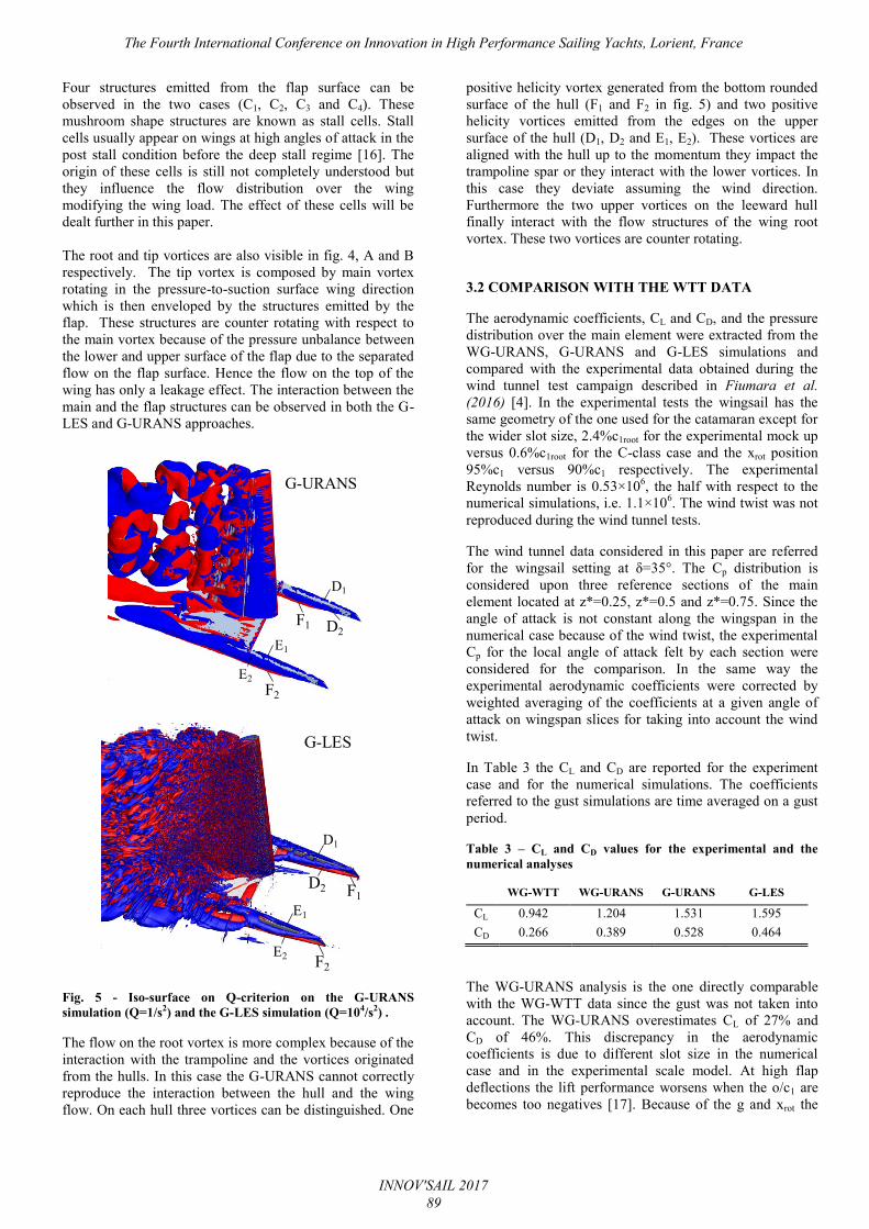
Four structures emitted from the flap surface can be

observed in the two cases (C1, C2, C3 and C4). These

mushroom shape structures are known as stall cells. Stall

cells usually appear on wings at high angles of attack in the

post stall condition before the deep stall regime [16]. The

origin of these cells is still not completely understood but

they influence the flow distribution over the wing

modifying the wing load. The effect of these cells will be

dealt further in this paper.

The root and tip vortices are also visible in fig. 4, A and B

respectively. The tip vortex is composed by main vortex

rotating in the pressure-to-suction surface wing direction

which is then enveloped by the structures emitted by the

flap. These structures are counter rotating with respect to

the main vortex because of the pressure unbalance between

the lower and upper surface of the flap due to the separated

flow on the flap surface. Hence the flow on the top of the

wing has only a leakage effect. The interaction between the

main and the flap structures can be observed in both the G-

LES and G-URANS approaches.

Fig. 5 - Iso-surface on Q-criterion on the G-URANS

simulation (Q=1/s2) and the G-LES simulation (Q=104/s2) .

The flow on the root vortex is more complex because of the

interaction with the trampoline and the vortices originated

from the hulls. In this case the G-URANS cannot correctly

reproduce the interaction between the hull and the wing

flow. On each hull three vortices can be distinguished. One

positive helicity vortex generated from the bottom rounded

surface of the hull (F1 and F2 in fig. 5) and two positive

helicity vortices emitted from the edges on the upper

surface of the hull (D1, D2 and E1, E2). These vortices are

aligned with the hull up to the momentum they impact the

trampoline spar or they interact with the lower vortices. In

this case they deviate assuming the wind direction.

Furthermore the two upper vortices on the leeward hull

finally interact with the flow structures of the wing root

vortex. These two vortices are counter rotating.

3.2 COMPARISON WITH THE WTT DATA

The aerodynamic coefficients, CL and CD, and the pressure

distribution over the main element were extracted from the

WG-URANS, G-URANS and G-LES simulations and

compared with the experimental data obtained during the

wind tunnel test campaign described in Fiumara et al.

(2016) [4]. In the experimental tests the wingsail has the

same geometry of the one used for the catamaran except for

the wider slot size, 2.4%c1root for the experimental mock up

versus 0.6%c1root for the C-class case and the xrot position

95%c1 versus 90%c1 respectively. The experimental

Reynolds number is 0.53×106, the half with respect to the

numerical simulations, i.e. 1.1×106. The wind twist was not

reproduced during the wind tunnel tests.

The wind tunnel data considered in this paper are referred

for the wingsail setting at δ=35°. The Cp distribution is

considered upon three reference sections of the main

element located at z*=0.25, z*=0.5 and z*=0.75. Since the

angle of attack is not constant along the wingspan in the

numerical case because of the wind twist, the experimental

Cp for the local angle of attack felt by each section were

considered for the comparison. In the same way the

experimental aerodynamic coefficients were corrected by

weighted averaging of the coefficients at a given angle of

attack on wingspan slices for taking into account the wind

twist.

In Table 3 the CL and CD are reported for the experiment

case and for the numerical simulations. The coefficients

referred to the gust simulations are time averaged on a gust

period.

Table 3 – CL and CD values for the experimental and the

numerical analyses

WG-WTT WG-URANS G-URANS G-LES

CL 0.942 1.204 1.531 1.595

CD 0.266 0.389 0.528 0.464

The WG-URANS analysis is the one directly comparable

with the WG-WTT data since the gust was not taken into

account. The WG-URANS overestimates CL of 27% and

CD of 46%. This discrepancy in the aerodynamic

coefficients is due to different slot size in the numerical

case and in the experimental scale model. At high flap

deflections the lift performance worsens when the o/c1 are

becomes too negatives [17]. Because of the g and xrot the

D1

D2F1

F2

E2

E1

G-URANS

D1

D2

E1

E2

F1

F2

G-LES


INNOV'SAIL 2017 89

o/c1 is negative on the experimental case, i.e. the flap L.E.

and the main T.E. are not overlapped, and positive on the

numerical case. Furthermore on the experimental mock-up

the o/c1 was even increased (in magnitude) during the tests

because of the wing deformation [5]. The deformation

involved in particular the high wing section modifying then

the flow physics on this zone and modifying the lift

performance of the wing.

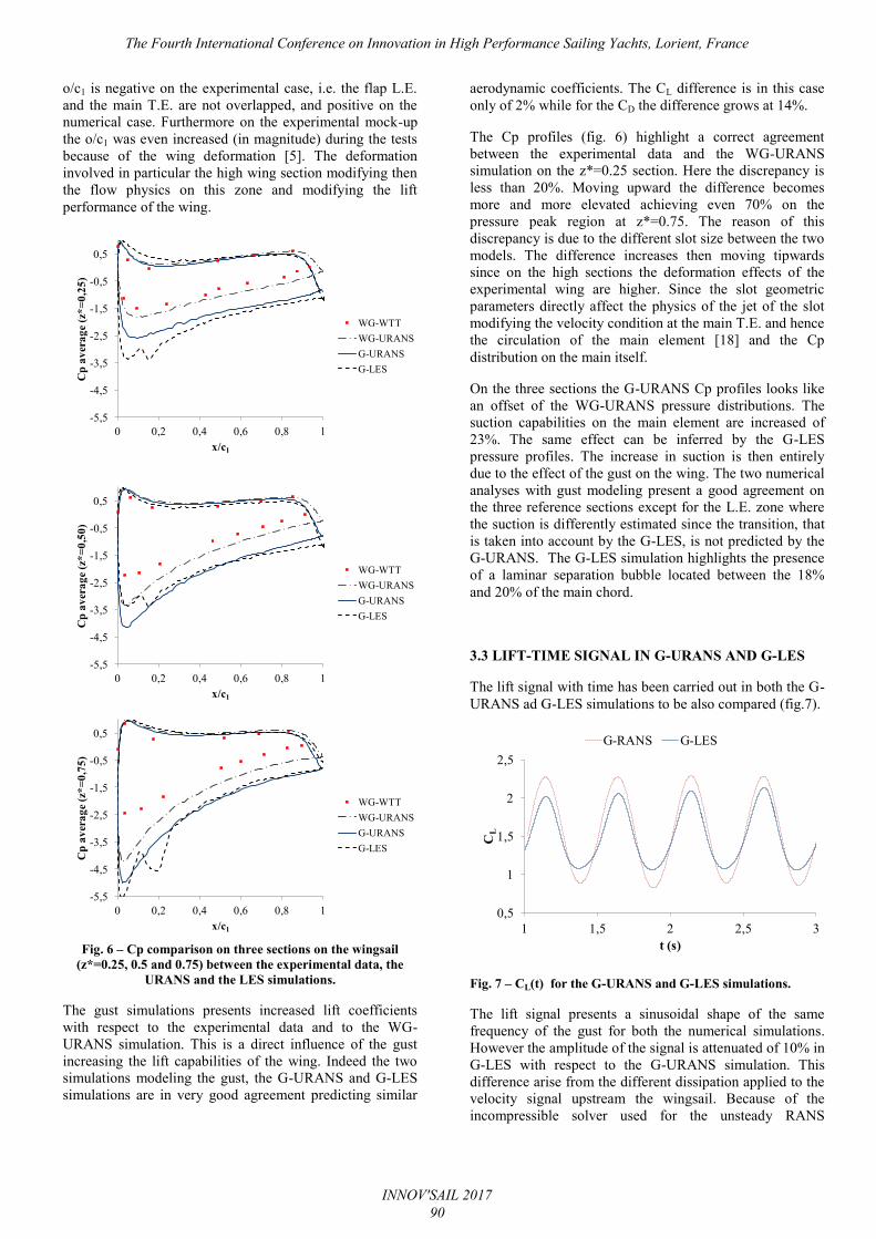
Fig. 6 – Cp comparison on three sections on the wingsail

(z*=0.25, 0.5 and 0.75) between the experimental data, the

URANS and the LES simulations.

The gust simulations presents increased lift coefficients

with respect to the experimental data and to the WG-

URANS simulation. This is a direct influence of the gust

increasing the lift capabilities of the wing. Indeed the two

simulations modeling the gust, the G-URANS and G-LES

simulations are in very good agreement predicting similar

aerodynamic coefficients. The CL difference is in this case

only of 2% while for the CD the difference grows at 14%.

The Cp profiles (fig. 6) highlight a correct agreement

between the experimental data and the WG-URANS

simulation on the z*=0.25 section. Here the discrepancy is

less than 20%. Moving upward the difference becomes

more and more elevated achieving even 70% on the

pressure peak region at z*=0.75. The reason of this

discrepancy is due to the different slot size between the two

models. The difference increases then moving tipwards

since on the high sections the deformation effects of the

experimental wing are higher. Since the slot geometric

parameters directly affect the physics of the jet of the slot

modifying the velocity condition at the main T.E. and hence

the circulation of the main element [18] and the Cp

distribution on the main itself.

On the three sections the G-URANS Cp profiles looks like

an offset of the WG-URANS pressure distributions. The

suction capabilities on the main element are increased of

23%. The same effect can be inferred by the G-LES

pressure profiles. The increase in suction is then entirely

due to the effect of the gust on the wing. The two numerical

analyses with gust modeling present a good agreement on

the three reference sections except for the L.E. zone where

the suction is differently estimated since the transition, that

is taken into account by the G-LES, is not predicted by the

G-URANS. The G-LES simulation highlights the presence

of a laminar separation bubble located between the 18%

and 20% of the main chord.

3.3 LIFT-TIME SIGNAL IN G-URANS AND G-LES

The lift signal with time has been carried out in both the G-

URANS ad G-LES simulations to be also compared (fig.7).

Fig. 7 – CL(t) for the G-URANS and G-LES simulations.

The lift signal presents a sinusoidal shape of the same

frequency of the gust for both the numerical simulations.

However the amplitude of the signal is attenuated of 10% in

G-LES with respect to the G-URANS simulation. This

difference arise from the different dissipation applied to the

velocity signal upstream the wingsail. Because of the

incompressible solver used for the unsteady RANS

-5,5

-4,5

-3,5

-2,5

-1,5

-0,5

0,5

0 0,2 0,4 0,6 0,8 1

Cp

av

era

ge

(z*

=0

,25

)

x/c1

WG-WTT

WG-URANS

G-URANS

G-LES

-5,5

-4,5

-3,5

-2,5

-1,5

-0,5

0,5

0 0,2 0,4 0,6 0,8 1

Cp

av

era

ge

(z*

=0

,50

)

x/c1

WG-WTT

WG-URANS

G-URANS

G-LES

-5,5

-4,5

-3,5

-2,5

-1,5

-0,5

0,5

0 0,2 0,4 0,6 0,8 1

Cp

av

era

ge

(z*

=0

,75

)

x/c1

WG-WTT

WG-URANS

G-URANS

G-LES

0,5

1

1,5

2

2,5

1 1,5 2 2,5 3

CL

t (s)

G-RANS G-LES


INNOV'SAIL 2017 90

simulation the signal propagation occurs instantaneously in

the flow domain while on the LES simulation, using a

compressible solver, the signal is convected from the

boundary domain to the wing. In this last case the signal

tends to be dissipated by the numerical scheme. In Table 4

the maximum and minimum velocities carried out 3 chords

upstream of the wingsail at z*=0.5 are reported for the two

numerical simulations.

Table 4 – Maximum and minimum adimensional velocity

measured at x=-3c, y=0, z*=0.5 for both the G-LES and G-

URANS simulations.

G-LES G-URANS Δ(%)

Max V/V∞ 1.07 1.198 11%

Min V/V∞ 0.96 0.875 10%

The velocity signal is more attenuated in the G-LES

simulation with the maximum and the minimum velocity

peaks that are respectively 10% and 11% smaller than in

the G-URANS analysis. This difference is of the same

order of the one estimated in the CL signal (10%) explained

the reason of the lift estimation with the two approaches.

3.4 FLOWFIELD COMPARISON BETWEEN THE G-

LES AND G-URANS SIMULATIONS

The flow of a multi-element wing is still difficult to model

because of the multi-layer structure of the flow in the

confluent boundary layer region over the flap surface. Here

the potential jet of the slot lies between two viscous layers,

i.e. the flap B.L. and the main wake. The three layers

interact in a way to form the confluent boundary layer

profile. If the slot is correctly designed the velocity profile

of the confluent boundary layer does not merge, i.e. it is

possible to distinguish the different velocity layers,

improving the flow possibilities to withstand the adverse

pressure gradients on the flap surface [18]. The confluent

boundary layer is highly sensitive to the effects of the

Reynolds number and the turbulence level making the

simulation of such a flow still complex.

Fiumara et al. (2016) [5] compared unsteady RANS

solutions with PIV data to investigate the limits of the

numerical means in the analysis of a two-element wingsail.

The velocity field was in good agreement while k was

sensibly underestimated by the numerical means. A

comparison between the G-LES and the G-URANS

analysis was then carried out on the velocity and the TKE

scalar maps on three wing sections located at z*=0.25,

z*=0.50 and z*=0.75. The scalar maps of the non-

dimensional averaged velocity V/V∞ on the flap surface of

the G-LES and G-URANS are reported in fig. 8. In both the

cases the flow separates from the flap surface in the

neighbors of the flap L.E. As a general statement in the G-

LES the separation takes place downstream of the L.E. On

the G-URANS case instead the separation occurs close to

the L.E. preventing any surrounding.

G-URANS G-LES

Fig. 8 – Comparison of the velocity field on the flap region for

the G-LES and G-URANS simulations for z*=75% (top), 50%

(middle) and 25% (bottom).

On the z*=0.25 section in the G-LES analysis the flow

reattaches at 40% of the flap chord forming a recirculation

bubble. The length of this bubble is instead underestimated

by the G-URANS simulation. The flow in this case

reattaches at 30%c2 for then separating again at 40%c2. On

the z*=0.5 and z*=0.75 the flow features of the two

analyses are more similar. Here the flow appeared separated

on the entire flap chord. However a recirculation zone can

also be distinguished on the flap surface. At z*=0.5 the

bubble is located on the mid-chord with an extent of 30%c2.

At z*=0.75 the bubble is located further downstream having

an extent of 40%c2.

In the G-LES simulation the k arises in the mixing layer

between the flap layer and the jet of the slot for then

spreading downstream (fig. 9). Particularly the mixing

layer between the jet and the flap B.L. is characterized by a

high level of k that is not reproduced by the G-URANS

simulation preventing the possibility of the flap L.E.

surrounding. The G-URANS analysis tends instead to

underestimate the k on the flap surface which is

concentrated only in the one of flow reattachment on the

flap surface.

V/V∞

0 0.9 1.50.3


INNOV'SAIL 2017 91

G-LES G-URANS

Fig. 9 – Comparison of the k on the flap region for the G-LES

and G-URANS simulations for z*=75% (top), 50% (middle)

and 25% (bottom).

4 WINGSAIL RESPONSE TO WIND GUST

The comparison between the G-URANS and G-LES

showed that both modeling approaches are in good

agreement. The unsteady URANS has furthermore the

advantage of a lower computational cost allowing the

possibility to perform parametric analyses. As observed in

the aerodynamic coefficient analysis the effect of the gust is

to improve the lift. However this enhancement depends on

the gust characteristics and varies with the gust frequency.

To better understand the influence of the gust oscillation on

the wingsail performance the unsteady RANS approach has

been then exploited to perform analyses of the gust

frequency effect.

4.1 LIFT MODIFICATION WITH THE GUST

The lift signals of the wingsail have been carried out for

each gust frequency analyzed. The averaged CL increases

with F+

with an improvement with respect to the WG-

URANS case of 1.7%, 19.4%, 27.1%, 38.3% and 26.1%

starting from the lower to the highest frequency (Fig. 10).

The maximum averaged lift is achieved for F+=1.246. The

maximum peak lift increases monotonically with the gust

frequency while the minimum peak lift increases up to

F+=0.312 for then reducing. The amplitude of the CL signal

amplifies then with the increase of the frequency.

Furthermore the reduction of the minimum lift becomes

more elevated at F+=2.492. In this case the CL lowers of

65% with respect to F+=1.246 while the difference in CL

between F+=1.246 and F

+=0.623 is only 10%.

Fig. 10 – Evolution with the gust frequency of the averaged CL

and the maximum and minimum peaks in CL.

Analyzing the load on the two wingsail elements, it can be

noticed that if in the maximum lift peak condition the CL

provided by the flap is about 40% at the different gust

frequencies, in the minimum peak lift the flap contribution

decreases more and more with the F+ increase (Fig. 11). At

F+=2.492 the flap provides even negative lift reducing then

the lift of the wingsail.

Fig. 11 – Flap lift with respect to the whole wingsail lift at the

different gust frequencies in the maximum and minimum

peaks conditions.

4.2 FLOW FEATURES MODIFICATION WITH THE

WIND GUST FREQUENCY

The gust frequency strongly affects the flow pattern over

the flap surface. In absence of gust, i.e. on the WG-URANS

simulation, the flow on the flap is completely separated.

The slot is indeed too wide to allow the jet of the slot to be

attached. The periodic oscillation due to the gust makes the

flow reattachment possible on the flap L.E. allowing stall

cells to form on the flap surface.

2k/V∞2

0 0.2 0.60.80.4

0

0,5

1

1,5

2

2,5

3

0 0,5 1 1,5 2 2,5

CL

F+

-60

-40

-20

0

20

40

60

0 0,5 1 1,5 2 2,5

CL

flap/C

L (%

)

F+

CL peak min CL peak max


INNOV'SAIL 2017 92

In fig.12 the evolution of the flow pattern on the flap

surface can be underlined at different F+. At low frequency

(F+=0.156) the flow is still separated on the flap surface and

it starts to locally reattach on the low flap sections when the

gust frequency achieves F+=0.312. Here two flow structures

take place on the low flap sections. At F+=0.623 the flow is

organized in cells regularly distributed on the wing span.

As already observed in the previous sections four stall cells

can be distinguished on the flap surface.

Fig. 12 – Skin friction colormaps on the wingsail upper surface

at different frequencies of the gust in the maximum peak lift

condition.

The increase of F+ modifies the span size of the stall cells

that tends to reduce while the number of cells appearing in

the flap increases. In particular between F+=0.623 and

F+=1.246 the number of stall cells doubles from 4 to 8

(Table 5). At F+=2.492 the number of cell increases at 12.

The extent of the region where the cells develop reduces

when increasing the frequency. The lower cell at F+=0.623

is located at z*=13% moving at 21.6% at F+=1.246 and

26% at F+=2.492.

Table 5 – Number of stall cells for each gust frequency.

F+ 0.156 0.312 0.623 1.246 2.492

N cells 0 2 4 8 12

4.3 STALL CELL PHYSICS

Stall cells usually form on wings after the onset of the stall.

They originate from a not uniform spanwise flow

separation starting from the wing T.E. The separation line

delimiting the attached flow from the separated one is not

parallel to the wing L.E. but assumes a wavy shape. As

described by Manolesos et al. (2014) a stall cell is made of

a vortex system composed by two counter rotating vortices

evolving in the chordwise direction (fig. 13), named SC

vortices, and two spanwise vortices, i.e. the separation line

(SL) and the T.E. vortices.

Fig. 13 – Stall cell structures from Manolesos et al. [19].

Despite stall cells are due to the occurrence of the flow

separation on the wingsail, instead, the stall cells are

originated from a flow re-attachment on the flap surface.

The flow reattaches locally at certain wing sections, on the

flap L.E. region forming a recirculation bubble.

Downstream of the bubble the flow separates again giving

the ability to a stall cell to form. In the flap zone adjacent to

the stall cell the flow cannot reattach and remains

separated.

These structures have a periodic evolution in the spanwise

direction. In fig. 14 the evolution of the flow on the wing

around z*=34.6% for F+=0.623 is showed. The cells are

completely formed on the flap surface when the maximum

peak lift condition is achieved. Then, they are convected

downstream leaving eventually the flap T.E. The

F+=0.156

F+=0.312

F+=0.623

F+=1.246

F+=2.492

0 0.01 0.02 0.03 0.04

CF

SC focus

Separation line

SL vortex

Symmetry plane

SC vortex

SL vortex

TE vortex

Symmetry plane


INNOV'SAIL 2017 93

recirculation bubble length increases extending toward the

flap T.E. At this moment the minimum peak lift is

achieved. Contemporary new stall cells start to form on the

flap L.E. in the zone where the flow was previously

completely separated.

When the maximum peak lift condition is achieved, the SC

vortices and the SL vortex flowing on the flap surface allow

local flow reattachment improving the lift flap capabilities

(Fig.15). The flap effectiveness increases with the gust

frequency so with the number of cells and of vortices. That

is the reason why the maximum lift peak increases with the

frequency.

Fig. 14 – Flow evolution over the flap surface in the span

region included between z*=30% and z*=39% for F+=0.632.

Isosurfaces on Q-criterion with vorticity scalar maps.

In the minimum peak lift condition the stall cells have no

more influence on the flap surface. In this condition the

only structure that can be detected on the flap is the

recirculation bubble. The bubble enlarges moving

streamwise toward the flap T.E. The remaining part of the

flow is instead separated (Fig 15). The bubble zone allows

reducing the loss of lift due to the flow separation since its

interior pressure remains constant. However the length of

the bubble shortens with the gust frequency reducing the

constant pressure region on the upper surface of the flap

decreasing then the lift brought by the flap. For the high

frequency F+=2.492 the laminar bubble is very small and

does not influence the flow pattern on the flap. At the same

a massive flow separation arises from the flap T.E. that is

not mitigated by any flow structure. This massive

separation abruptly increases the flap load on leading even

to a negative lift (Fig 11).

Separated

flow Recirculation

bubble Attached flow

Fig. 15 – Instantaneous flow pattern on the wing surface at

F+=0.623 in the maximum and minimum lift conditions.

The gust frequency is the origin of the flow reattachment on

the flap L.E. region leading the possibility to the stall cell to

form on the flap surface. The periodic movement of the

gust leads to a jet pulsation in the slot region which acts

similarly to flow separation control devices adopted in

some high-lift configurations.

However the reattachment characteristics depend on two

main parameters, the frequency of the pulsation and the

momentum provided by the jet of the slot. This effect is

deeply analyzed in the next section.

4.4 FLOW REATTACHMENT BY JET PULSATION

The influence of pulsed jet to achieve flow reattachment

over a deflected flap was deeply studied by Nishri et al.

(1998) [19]. Starting from a fully separated flow a jet

pulsation allows the flow reattachment if the jet blows in a

range of frequencies providing a velocity momentum higher

than the one of the reattachment threshold. To express the

momentum the Cµ=2Vj2yF/(V∞

2c2) is introduced where Vj

is the averaged velocity in the slot. Both the frequency

range and the minimum momentum coefficient allowing

flow reattachment are dependent on Re and length scale

ratio yF/c2. In fig. 11 the threshold curve for the Cµ carried

out by Nishri et al. is represented. The curves represent the

minimum Cµ required at each frequency to reattach the

flow over a flap deflected 8° more than the separation

deflection angle.

Peak max CL

SC vortices

SL vortex

Peak min CL

Peak max CL

X-vorticity (/s)

30-30 -18 -6 6 180

CLmax

CLmin


INNOV'SAIL 2017 94

The range of frequencies at which the flow reattachment is

effective reduces with the increase of the slot size and the

Cµ required at a given frequency increases too. However in

the range of frequency 1.2<F+<1.5 the minimum Cµ

condition is independent on these two parameters. The

F+=1.249, the one that maximize the averaged lift of the

wing is exactly inside this frequency range. Nevertheless,

even at the correct frequency, the Cµ is not sufficient to

provide a flow reattachment on the flap. At this slot

condition indeed the flow separates even for flap deflection

lower than 25°, 10° less than the flap deflection angle of the

wingsail analyzed in this paper. At F+=0.156, the condition

at which the flow remains separated on the flap surface, the

frequency is too small even for small slot size to allow a

flow reattachment. The local flow attachment on the

wingsail was observed in the range of frequency between

0.623 and 2.492. Even in this case the flow reattachment

was not complete because of the too small Cµ.

Fig. 16 – Averaged Cµ points for the wingsail at different

frequencies on two spanwise locations on the minimal

reattached curves carried out by Nishri et al. (1998) [20].

In the reattachment process the flow encloses a dead air

region forming the recirculation bubble described in the

previous section. The length of this bubble reduces with the

increase of Cµ or F+ [20][21]. This is consistent with the

observations made in the previous section.

The physics of the bubble affects the following separation.

At low frequencies the flow separates because of the bubble

burst mechanism reducing the flap effectiveness. However

at higher frequencies, i.e. F+=2.8 [20], the bubble

completely disappears with the separation that starts from

the flap T.E. zone due to the thickening of the boundary

layer. Hence by increasing the frequency, the flow

separation does not occur by bubble burst but instead by

flow separation from the T.E. This is the case for the

F+=2.492 case. The massive separated zone largely

decreases the flap effectiveness.

At F+=1.246 the extent of the separated zone on the T.E.

zone reduces. At F+=0.632 instead the flow separation

occurs by burst of the recirculation bubble especially in the

zone in the middle of the stall cell. Here the momentum is

the lower one so that the bubble length enlarges up to burst.

5 CONCLUSIONS

Numerical analyses were carried out on a C-class

catamaran in downwind condition modeling the wind twist

and gust. A LES and an unsteady RANS approach were

adopted for the simulations.

The results of the two simulations agree well. The

aerodynamic coefficients are in good agree and the Cp

distribution on the main element are also comparable

except the L.E. region where the transition in the unsteady

RANS is not taken into account. The scale maps also are in

agreement while unsteady RANS analysis tends to

underestimate turbulent kinetic energy. In both analyses

stall cells can be observed on the flap surface. The origin of

these cells depends on the flow re-attachment on the flap

caused by the gust pulsation in the slot region.

Modifying the gust frequency in the URANS analysis a

remarkable modification of the lift coefficient of the wing

can be observed. The averaged and amplitude variation of

CL tends to increase with the gust frequency. This

improvement of the lift performance is linked to the stall

cells on the flap surface.

The streamwise vortices emerging from the stall cells allow

the flow reattachment on the flap. Due to the size reduction

of the cells with the gust frequency and the augmentation of

their number of the flap, the attached surface enlarges more

and more increasing the flap effectiveness.

However in the minimum lift condition the stall cells are

dissipated. The lift improvement is only due to a

recirculation bubble extending on the flap surface while the

flow is completely separated. The bubble shortens with the

frequency increase reducing the lift capabilities of the wing.

ACKNOWLEDGMENTS

This research is supported in part by ASSYSTEM France,

which kindly provided PhD funding.

Acknowledgments to the support provided by the

computing center of the University of Toulouse (CALMIP).

References

[1] Magherini, M., Turnock, S.R., Campbell, I.M. (2014),

“Parameters Affecting the Performance of the C-Class Wingsail”,

TRANS. RINA: IJSCT, Vol 156, Part B1, 21-34, 2014.

[2] Blakeley, A.W., Flay, R.G.J., Richards, P.J. (2012), “Design

and Optimisation of Multi-Element Wing Sails for Multihull

Rec2=3 105 yF/c2=0.6%

Cµ

( 105)

F+

1 2 30

10

20

30

40

50

Rec2=3 105 yF/c2=1.0%

2.4921.2460.623

0.3120.156

z*=34.6% z*=69.2%


INNOV'SAIL 2017 95

Yachts”, 18th Australasian Fluid Mechanics Conference,

Launcestion, Australia, 3-7 December 2012.

[3] Blakeley, A.W., Flay, R.G.J., Furukawa, H., Richards, P.J.

(2015), “Evaluation of multi-element wingsail aerodynamics from

Two-dimensional wind tunnel Investigations”, 5th High

Performance Yacht Design Conference, Auckland, 10-12 March,

2015.

[4] Chapin, V., Gourdain, N., Verdin, N., Fiumara, A., Senter, J.

(2015),” Aerodynamic study of a two-elements wingsail for high

performance multihull yachts”, 5th High Performance Yacht

Design Conference, Auckland, 10-12 March, 2015.

[5] Fiumara, A., Gourdain, N., Chapin, V., Senter, J., Bury, Y.

(2015), “Numerical and experimental Analysis of the flow around

a Two-Element Wingsail at Reynolds Number 0.53×106”, Int. J.

Heat Fluid Flow.

[6] Fiumara, A., Gourdain, N., Chapin, V., Senter, J. (2016),

“Aerodynamic Analysis of 3D Multi-Element Wings: an

Application to Wingsails of Flying Boats”, RAeS, Conference

Paper, Bristol UK, 19-21 July, 2016.

[7] Viola, I.M., Bartesaghi S., Van-Renterghem, T., Ponzini, R.

(2014), “Detached Eddy Simulation of a Sailing Yacht”, Ocean

Engineering, 90, 93-103, 2014.

[8] Deck, S. (2005), “Zonal-Detached-Eddy Simulation of the

Flow around a High-Lift Configuration”, AIAA Journal, Vol. 43,

No. 11, 2372-2384, November 2005.

[9] Deck, S., Laraufie, R. (2013), “Numerical Investigation of the

flow Dynamics past a three-element aerofoil”, J. Fluid Mech., Vo.

732, 401-444, 2013.

[10] Beaupuits, J.P.P., Otárola, A., Rantakyrö, F.T., River, R.C.,

Radford, S.J.E., Nyman, L-Å (2004), “Analysis of Wind Data

Gathered at Chajnantor”, ALMA Memo No. 467.

[11] Shiau, B.S., Chen, Y.B. (2002), “Observation in Wind Tunnel

characteristics and Velocity Spectra near the Ground at the coastal

Region”, J. of Wind Eng. and Ind. Aerodynamics, 90, 1671-1681,

2002.

[12] Menter, F.R. (1994), “Two-equation eddy-viscosity

turbulence models for engineering applications”, AIAA J. Vol. 32,

No. 8 (1994), pp.1598-1605.

[13] Bermejo-Moreno, I., Bodart, J., Larsson, J., Barney, B.M.,

Nichols, J.W., Jones, S. (2013), “Solving the compressible Navier-

Stokes equations on up to 1.97 Million cores and 4.1 trillion

points”, SC’2013: Proceedings in the International Conference on

High Performance Computing, Networking, Storage and Analysis.

[14] Vreman A. W. (2004), "An eddy-viscosity subgrid-scale

model for turbulent shear flow: Algebraic theory and

applications", Phys. Fluids 16, 3670-3681 (2004).

[15] Kawai, S., Larsson, J. (2012), “Wall-modeling in large eddy

simulation: Length scales, grid resolution, and accuracy”, Phys.

Fluids, Vol. 24, December 2011.

[16] Yon, S., Katz, J. (1997), Study of the unsteady flow features

on a stalled wing”, AIAA paper 97-1927.

[17] Woodward, D.S., Lean, D.E., (1993), “Where is the high lift

today? A review of past UK research programs”. AGARD-CP515.

[18] Smith, A.M.O. (1975), “High-Lift Aerodynamics”, J. of

Aircraft, 12(6), 501-530.

[19] Manolesos, M., Voutsinas, S. G. (2014), “Study of a stall cell

using stereo particle image velocimetry”, Phys. Fluids 26,

045101 (2014).

[20] Nishri, B., Wygnanski, I. (1998), “Effects of periodic

excitation on turbulent separation from a flap”, AIAA J., 1998,

Vol. 36, No. 4.

[21] Greenblatt, D., Wygnanski, I.J. (2000), “The control of flow

separation by periodic excitation”, Progress in Aerospace Sciences

36 (2000), pp. 487-545

AUTHORS BIOGRAPHY

Alessandro Fiumara is Ph.D. candidate in fluid mechanics

for the Wingsail project promoted by Assystem France and

ISAE-Supaéro. Aeronautical engineer from ISAE-Supaéro

and the University of Rome “Sapienza”, he has experience

in numerical and experimental aerodynamics.

Nicolas Gourdain is full professor at the aerodynamic,

energetic and propulsion department (DAEP) of ISAE-

Supaéro since 2013. PhD in fluid mechanics from the Ecole

Centrale de Lyon (2005) he joined the CFD team at

CERFACS in Toulouse in 2006 as senior researcher.

Vincent G. Chapin is Associate Professor at ISAE since

1993. In charge of Low Speed Aerodynamics, he has long

experience in high speed sailing with patent pending. He

has studied the innovative twin-rig of the Hydraplaneur of

Y. Parlier, developed evolutionary optimization applied in

aerodynamics or multidisciplinary problems. In 2017, he

has proposed a new lecture on wind propulsion of flying

boats at ISAE-SUPAERO.

Julien Senter is the manager of the Fluid Dynamics team

of Assystem France. Dr. Engineer from Ecole Centrale

Nantes (2006) and Ensiame (2003), he has more than 10

years of experience in the industry for major clients in

various sectors (aerospace, energy, automotive...). He is

passionate about the world sailing.


INNOV'SAIL 2017 96

aerodynamic analysis around a c-class catamaran in...

Documents