1

Adaptive Image Denoising by Mixture AdaptationEnming Luo, Student Member, IEEE, Stanley H. Chan, Member, IEEE, and Truong Q. Nguyen, Fellow, IEEE

Abstract—We propose an adaptive learning procedure to learnpatch-based image priors for image denoising. The new algo-rithm, called the Expectation-Maximization (EM) adaptation,takes a generic prior learned from a generic external databaseand adapts it to the noisy image to generate a specific prior.Different from existing methods that combine internal andexternal statistics in ad-hoc ways, the proposed algorithm isrigorously derived from a Bayesian hyper-prior perspective.There are two contributions of this paper: First, we providefull derivation of the EM adaptation algorithm and demonstratemethods to improve the computational complexity. Second, in theabsence of the latent clean image, we show how EM adaptationcan be modified based on pre-filtering. Experimental results showthat the proposed adaptation algorithm yields consistently betterdenoising results than the one without adaptation and is superiorto several state-of-the-art algorithms.

Index Terms—Image Denoising, Hyper Prior, Conjugate Prior,Gaussian Mixture Models, Expectation-Maximization (EM), Ex-pected Patch Log-Likelihood (EPLL), EM Adapation, BM3D

I. INTRODUCTION

A. Overview

We consider the classical image denoising problem: Given

an additive i.i.d. Gaussian noise model,

y = x+ ε, (1)

our goal is to find an estimate of x from y, where x ∈ Rn

denotes the (unknown) clean image, ε ∼ N (0, σ2I) ∈ Rn

denotes the Gaussian noise vector with zero mean and co-

variance matrix σ2I (where I is the identity matrix), and

y ∈ Rn denotes the observed noisy image.

Image denoising is a long-standing problem. Over the

past few decades, numerous denoising algorithms have been

proposed, ranging from spatial domain methods [1–3] to

transform domain methods [4–6], and from local filtering [7–

9] to global optimization [10, 11]. In this paper, we focus on

the Maximum a Posteriori (MAP) approach [11, 12]. MAP

is a Bayesian approach which tackles image denoising by

maximizing the posterior probability

argmaxx

f(y|x)f(x) = argminx

{1

2σ2‖y − x‖2 − log f(x)

}.

E. Luo and T. Nguyen are with the Department of Electrical and ComputerEngineering, University of California at San Diego, La Jolla, CA 92093, USA.(emails: eluo@ucsd.edu and nguyent@ece.ucsd.edu).

S. Chan is with the School of Electrical and Computer Engineering, andthe Department of Statistics, Purdue University, West Lafayette, IN 47907,USA. (email: stanleychan@purdue.edu).

This work was supported by the National Science Foundation under grantCCF-1065305 and by DARPA under contract W911NF-11-C-0210. Prelimi-nary material in this paper was presented at the 3rd IEEE Global Conferenceon Signal & Information Processing (GlobalSIP), Orlando, December, 2015.

This paper follows the concept of reproducible research. All the results andexamples presented in the paper are reproducible using the code and imagesavailable online at http://videoprocessing.ucsd.edu/~eluo.

Here, the first term is a quadratic function due to the Gaussian

noise model. The second term is the negative log of the image

prior. The benefit of using the MAP framework is that it

allows us to explicitly formulate our prior knowledge about

the image via the distribution f(x).The success of an MAP optimization depends vitally on

the modeling capability of the prior f(x) [13–15]. However,

seeking f(x) for the whole image x is practically impossible

because of the high dimensionality. To alleviate the problem,

we adopt the common wisdom to approximate f(x) using a

collection of small patches. Such prior is known as the patch

prior, which is broadly attributed to Buades et al. for the non-

local means [16], and to an independent work of Awate and

Whitaker presented at the same conference [17]. (See [18] for

additional discussions about patch priors.) Mathematically, by

letting P i ∈ Rd×n be a patch-extract operator that extracts

the i-th d-dimensional patch from the image x, a patch prior

expresses the negative logarithm of the prior as a sum of the

logarithms, leading to

argminx

{1

2σ2‖y − x‖2 −

1

n

n∑

i=1

log f(P ix)

}. (2)

The prior thus formed is called the expected patch log

likelihood (EPLL) [11].

B. Related Work

Assuming that f(P ix) takes a parametric form for analytic

tractability, the question now becomes where to find training

samples and how to train the model. There are generally

two approaches. The first approach is to learn f(P ix) from

the single noisy image. We refer to these types of priors as

internal priors, e.g., [19]. The second approach is to learn

f(P ix) from a database of images. We call these types of

priors as external priors, e.g., [9, 20–23].

Combining internal and external priors has been an active

direction in recent years. Most of these methods are based on

a fusion approach, which attempts to directly aggregate the

results of the internal and the external statistics. For example,

Mosseri et al. [20] used a patch signal-to-noise ratio as a

metric to decide if a patch should be denoised internally or

externally; Burger et al. [21] applied a neural network to

weight the internal and external denoising results; Yue et al.

[24] used a frequency domain method to fuse the internal

and external denoising results. There are also some works

attempting to use external databases as a guide to train internal

priors [25, 26].

When f(P ix) is a Gaussian mixture model, there are spe-

cial treatments to optimize the performance, e.g., a framework

proposed by Awate and Whitaker [27–29]. In this method,

2

a simplified Gaussian mixture (using the same weights and

shared covariances) is learned directly from the noisy data

through an empirical Bayes framework. However, the method

primarily focuses on MRI data where the noise is Rician. This

is different from the i.i.d. Gaussian noise assumption in our

problem. The learning procedure is also different from ours

as we use an adaptation process to adapt the generic prior to

a specific prior. Our proposed method is inspired by the work

of Gauvain and Lee [30] with a few important modifications.

We should also mention the work of Weissman et al.

on universal denoising [31, 32]. Universal denoisers are a

general class of denoising algorithms that do not require

explicit knowledge about the prior and are also asymptotically

optimal. While not explicitly proven, patch-based denoising

methods such as non-local means [33] and BM3D [4] satisfy

these properties. For example, the asymptotic optimality of

non-local means was empirically verified by Levin et al. [34,

35] with computational improvements by Chan et al. [36].

However, we shall not discuss universal denoisers in detail as

they are beyond the scope of this paper.

C. Contribution and Organization

Our proposed algorithm is call EM adaptation. Like many

external methods, we assume that we have an external

database of images for training. However, we do not simply

compute the statistics of the external database. Instead, we

use the external statistics as a “guide” for learning the internal

statistics. As will be illustrated in the subsequent sections, this

can be formally done using a Bayesian framework.

This paper is an extension of our previous work reported

in [37]. This paper adds the following two new contributions:

1) Derivation of the EM adaptation algorithm. We rig-

orously derive the proposed EM adaptation algorithm

from a Bayesian hyper-prior perspective. Our derivation

complements the work of Gauvain and Lee [30] by

providing additional simplifications and justifications to

reduce computational complexity. We further provide

discussion of the convergence.

2) Handling of noisy data. We provide detailed discussion

of how to perform EM adaptation for noisy images. In

particular, we demonstrate how to automatically adjust

the internal parameters of the algorithm using pre-

filtered images.

When this paper was written, we became aware of a very

recent work by Lu et al. [38]. Compared to [38], this paper

provides theoretical results that are lacking in [38]. Numerical

comparisons can be found in the experiment section.

The rest of the paper is organized as follows: Section II

gives a brief review of the Gaussian mixture model. Section

III presents the proposed EM adaptation algorithm. Section

IV discusses how the EM adaptation algorithm should be

modified when the image is noisy. Experimental results are

presented in Section V.

II. MATHEMATICAL PRELIMINARIES

A. GMM and MAP Denoising

For notational simplicity, we shall denote pidef= P ix ∈ R

d

as the i-th patch from x. We say that pi is generated from a

Gaussian mixture model (GMM) if

f(pi |Θ) =K∑

k=1

πkN (pi|µk,Σk), (3)

where∑K

k=1 πk = 1 with πk being the weight of the k-th

Gaussian component, and

N (pi|µk,Σk) (4)

def=

1

(2π)d/2|Σk|1/2exp(−

1

2(pi − µk)

TΣ

−1k (pi − µk)

)

is the k-th Gaussian distribution with mean µk and covariance

Σk. We denote Θdef= {(πk,µk,Σk)}Kk=1 as the GMM

parameter.

With the GMM defined in (3), we can specify the denoising

procedure by solving the optimization problem in (2). Here,

we follow [39, 40] by using the half quadratic splitting strat-

egy. The idea is to replace (2) with the following minimization

argminx,{vi}n

i=1

{1

2σ2‖y − x‖2

+1

n

n∑

i=1

(− log f(vi) +

β

2‖P ix− vi‖

2)}

, (5)

where {vi}ni=1 are some auxiliary variables and β is a penalty

parameter. By assuming that f(vi) is dominated by the mode

of the Gaussian mixture, the solution to (5) is given in the

following proposition.

Proposition 1: Assuming f(vi) is dominated by the k∗i -th

components, where k∗idef= argmax

kπkN (vi|µk,Σk), the solu-

tion of (5) is

x =(nσ−2I + β

n∑

i=1

P Ti P i

)−1(nσ−2y + β

n∑

i=1

P Ti vi

),

vi =(βΣk∗

i+ I

)−1(µk∗

i

+ βΣk∗

iP ix

).

Proof: See [11].

Proposition 1 is a general procedure for denoising images

using a GMM under the MAP framework. There are, of

course, other possible denoising procedures that also use

GMM under the MAP framework, e.g., using surrogate meth-

ods [41]. However, we will not elaborate on these options. Our

focus is on how to obtain the GMM.

B. EM Algorithm

The GMM parameter Θ = {(πk,µk,Σk)}Kk=1 is typically

learned using the Expectation-Maximization (EM) algorithm.

EM is a known method. Interested readers can refer to [42]

for a comprehensive tutorial. For image denoising, we note

that the EM algorithm has several shortcomings as follows:

3

1) Adaptivity. For a fixed image database, the GMM

parameters are specifically trained for that particular

database. We call it the generic parameter. If, for ex-

ample, we are given an image that does not necessarily

belong to the database, then it becomes unclear how

one can adapt the generic parameter to the image.

2) Computational cost. Learning a good GMM requires

a large number of training samples. For example, the

GMM in [11] is learned from 2,000,000 randomly sam-

pled patches. If our goal is to adapt a generic parameter

to a particular image, then it would be more desirable

to bypass the computationally intensive procedure.

3) Finite samples. When training samples are few, the

learned GMM will be over-fitted; some components

will even become singular. This problem needs to be

resolved because a noisy image contains much fewer

patches than a database of patches.

4) Noise. In image denoising, the observed image always

contains noise. It is not clear how to mitigate the noise

while running the EM algorithm.

III. EM ADAPTATION

The proposed EM adaptation takes a generic prior and

adapts it to create a specific prior using very few samples.

Before giving the details of the EM adaptation, we first

provide a toy example to illustrate the idea.

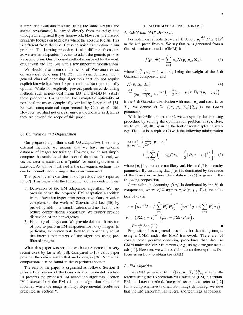
A. Toy Example

Suppose we are given two two-dimensional GMMs with

two clusters in each GMM. From each GMM, we syntheti-

cally generate 400 data points with each point representing

a 2D coordinate shown in Figure 1 (a) and (b). Imagine that

the data points in (a) come from an external database whereas

the data points in (b) come from a clean image of interest.

With the two sets of data, we apply EM to learn GMM 1

and GMM 2. Since we have enough samples, both GMMs are

estimated reasonably well as shown in (a) and (b). However,

if we reduce the number of points in (b) to 20, then learning

GMM 2 becomes problematic as shown in (c). Therefore, the

question is this: Suppose we are given GMM 1 and only 20

data points from GMM 2, is there a way that we can transfer

GMM 1 to the 20 data points so that we can approximately

estimate GMM 2? This is the goal of EM adaptation. A result

for this example is shown in (d).

B. Bayesian Hyper-prior

As illustrated in the toy example, what EM adaptation does

is to use the generic model parameters as a “guide” when

learning the new model parameters. Mathematically, suppose

{p̃1, . . . , p̃n} are patches from a single image parameterized

by a GMM with a parameter Θ̃def= {(π̃k, µ̃k, Σ̃k)}

Kk=1.

Our goal is to estimate Θ̃ with the aid of some generic

GMM parameter Θ. However, in order to formally derive the

algorithm, we need to explain a Bayesian learning framework.

−6 −4 −2 0 2 4 6−6

−4

−2

0

2

4

6

−6 −4 −2 0 2 4 6−6

−4

−2

0

2

4

6

(a) GMM 1 / 400 points (b) GMM 2 / 400 points

−6 −4 −2 0 2 4 6−6

−4

−2

0

2

4

6

−6 −4 −2 0 2 4 6−6

−4

−2

0

2

4

6

(c) GMM 2 / 20 points (d) Adapted / 20 points

Fig. 1: (a) and (b), Two GMMs, each learned using the EM

algorithm from 400 data points of 2D coordinates. (c): A

GMM learned from a subset of 20 data points drawn from

(b). (d): An adapted GMM using the same 20 data points in

(c). Note the significant improvement from (c) to (d) by using

the proposed adaptation.

From a Bayesian perspective, estimation of the parameter

Θ̃ can be formulated as

Θ̃ = argmaxΘ̃

log f(Θ̃ | p̃1, . . . , p̃n)

= argmaxΘ̃

{log f(p̃1, . . . , p̃n | Θ̃) + log f(Θ̃)

}, (6)

where

f(p̃1, . . . , p̃n | Θ̃) =

n∏

i=1

{K∑

k=1

π̃kN (p̃i|µ̃k, Σ̃k)

}

is the joint distribution of the samples, and f(Θ̃) is some prior

of Θ̃. We note that (6) is also a MAP problem. However, the

MAP for (6) is the estimation of the model parameter Θ̃,

which is different from the MAP for denoising used in (2).

Although the difference seems subtle, there is a drastically

different implication that we should be aware of.

In (6), f(p̃1, . . . , p̃n | Θ̃) denotes the distribution of a

collection of patches conditioned on the parameter Θ̃. It is

the likelihood of observing {p̃1, . . . , p̃n} given the model

parameter Θ̃. f(Θ̃) is a distribution of the parameter, which

is called hyper-prior in machine learning [43]. Since Θ̃ is the

model parameter, the hyper-prior f(Θ̃) defines the probability

density of Θ̃.

Same as the usual Bayesian modeling, hyper-priors are

chosen according to a subjective belief. However, for efficient

computation, hyper-priors are usually chosen as the conjugate

priors of the likelihood function f(p̃1, . . . , p̃n | Θ̃) so that

the posterior distribution f(Θ̃ | p̃1, . . . , p̃n) has the same

4

functional form as the prior distribution. For example; Beta

distribution is a conjugate prior for a Bernoulli likelihood

function; Gaussian distribution is a conjugate prior for a likeli-

hood function that is also Gaussian, etc. For more discussions

on conjugate priors, we refer the readers to [43].

C. f(Θ̃) for GMM

For GMM, no joint conjugate prior can be found through

the sufficient statistic approach [30]. To allow tractable com-

putation, it is necessary to separately model the mixture

weights and the means/covariances by assuming that the

weights and means/covariances are independent.

We model the mixture weights as a multinomial distribution

so that the corresponding conjugate prior for the mixture

weight vector (π̃1, · · · , π̃K) is a Dirichlet density

π̃1, · · · , π̃K ∼ Dir(v1, · · · , vk), (7)

where vi > 0 is a pseudo-count for the Dirichlet distribution.

For mean and covariance (µ̃k, Σ̃k), the conjugate prior is

the normal-inverse-Wishart density so that

(µ̃k, Σ̃k) ∼ NIW(ϑk, τk,Ψk, ϕk), for k = 1, · · · ,K, (8)

where (ϑk, τk,Ψk, ϕk) are the parameters for the normal-

inverse-Wishart density such that ϑk is a vector of dimension

d, τk > 0, Ψk is a d × d positive definite matrix, and ϕk >d− 1.

Remark 1: The choice of the normal-inverse-Wishart dis-

tribution is important here, for it is the conjugate prior of

a multivariate normal distribution with unknown mean and

unknown covariance matrix. This choice is slightly different

from [30] where the authors choose a normal-Wishart distribu-

tion. While both normal-Wishart and normal-inverse-Wishart

can lead to the same result, the proof using normal-inverse-

Wishart is considerably simpler for its inverted matrices.

Assuming π̃k is independent of (µ̃k, Σ̃k), we factorize

f(Θ̃) as a product of (7) and (8). By ignoring the scaling

constants, it is not difficult to show that

f(Θ̃) ∝∏K

k=1

{π̃vk−1k |Σ̃k|

−(ϕk+d+2)/2

exp(− τk

2 (µ̃k − ϑk)TΣ̃

−1

k (µ̃k − ϑk)−12 tr(ΨkΣ̃

−1

k ))}

.

(9)

The importance of (9) is that it is a conjugate prior

of the complete data. As a result, the posterior density

f(Θ̃|p̃1, . . . , p̃n) belongs to the same distribution family as

f(Θ̃). This can be formally described in Proposition 2.

Proposition 2: Given the prior in (9), the posterior

f(Θ̃|p̃1, . . . , p̃n) is given by

f(Θ̃ | p̃1, . . . , p̃n) ∝∏K

k=1

{π̃v′

k−1

k |Σ̃k|−(ϕ′

k+d+2)/2

exp(− τ ′

k

2

(µ̃k − ϑ′

k

)TΣ̃

−1

k

(µ̃k − ϑ′

k

)− 1

2 tr(Ψ′kΣ̃

−1

k ))}

(10)

where

v′k = vk + nk, ϕ′k = ϕk + nk, τ ′k = τk + nk,

ϑ′k =

τkϑk + nkµ̄k

τk + nk,

Ψ′k = Ψk + Sk +

τknk

τk + nk(ϑk − µ̄k)(ϑk − µ̄k)

T ,

µ̄k =1

nk

n∑

i=1

γkip̃i, Sk =

n∑

i=1

γki(p̃i − µ̄k)(p̃i − µ̄k)T

are the parameters for the posterior density.

Proof: See Appendix A.

D. Solve for Θ̃

Solving for the optimal Θ̃ is equivalent to solving the

following optimization problem:

maximizeΘ̃

L(Θ̃)def= log f(Θ̃|p̃1, . . . , p̃n)

subject to∑K

k=1 π̃k = 1.(11)

The constrained problem (11) can be solved by considering

the Lagrange function and taking derivatives with respect

to each individual parameter. We summarize the optimal

solutions in Proposition 3.

Proposition 3: The optimal (π̃k, µ̃k, Σ̃k) for (11) are

π̃k =n

(∑K

k=1 vk −K) + n·nk

n

+

∑Kk=1 vk −K

(∑K

k=1 vk −K) + n·

vk − 1∑K

k=1 vk −K, (12)

µ̃k =1

τk + nk

n∑

i=1

γkip̃i +τk

τk + nkϑk, (13)

Σ̃k =nk

ϕk + d+ 2 + nk

1

nk

n∑

i=1

γki(p̃i − µ̃k)(p̃i − µ̃k)T

+1

ϕk + d+ 2 + nk

(Ψk + τk(ϑk − µ̃k)(ϑk − µ̃k)

T).

(14)

Proof: See Appendix B.

Remark 2: The results we showed in Proposition 3 are

different from [30]. In particular, the denominator for Σ̃k in

[30] is ϕk−d+nk whereas ours is ϕk+d+2+nk. However,

by using the simplification described in the next subsection,

we can obtain the same result for both cases.

E. Simplification of Θ̃

The results in Proposition 3 are general expressions for any

hyper-parameters. We now discuss how to simplify the result

with the help of the generic prior. First, since vk−1∑K

k=1vk−K

is

the mode of the Dirichlet distribution, a good surrogate for

it is πk. Second, ϑk denotes the prior mean in the normal-

inverse-Wishart distribution and thus can be appropriately ap-

proximated by µk. Moreover, since Ψk is the scale matrix on

Σ̃k and τk denotes the number of prior measurements in the

5

normal-inverse-Wishart distribution, they can be reasonably

chosen as Ψk = (ϕk + d + 2)Σk and τk = ϕk + d + 2.

Plugging these approximations in the results of Proposition

3, we summarize the simplification results as follows:

Proposition 4: Define ρdef= nk

n (∑K

k=1 vk − K) = τk =ϕk + d+ 2. Let

ϑk = µk, Ψk = (ϕk + d+ 2)Σk,vk − 1

∑Kk=1 vk −K

= πk,

and αk = nk

ρ+nk

, then (12)-(14) become

π̃k =αknk

n+ (1 − αk)πk, (15)

µ̃k =αk1

nk

n∑

i=1

γkip̃i + (1− αk)µk, (16)

Σ̃k = αk1

nk

n∑

i=1

γki(p̃i − µ̃k)(p̃i − µ̃k)T

+ (1− αk)(Σk + (µk − µ̃k)(µk − µ̃k)

T). (17)

Remark 3: We note that Reynold et al. [44] presented

similar simplification results (without derivations) as ours.

However, their results are valid only for the scalar case or

when the covariance matrices are diagonal. In contrast, our

results support full covariance matrices and thus are more

general. As will be seen, for our denoising application, since

the image pixels (especially adjacent pixels) are correlated, the

full covariance matrices are necessary for good performance.

Remark 4: Comparing (17) with the work of Lu et al. [38],

we note that in [38] the covariance is

Σ̃k = αk1

nk

n∑

i=1

γkip̃ip̃Ti + (1− αk)Σk. (18)

This result, although it looks similar to ours, is generally not

valid if we follow the Bayesian hyper-prior approach, unless

µk and µ̃k are both 0.

F. EM Adaptation Algorithm

The proposed EM adaptation algorithm is summarized in

Algorithm 1. EM adaptation shares many similarities with the

standard EM algorithm. To better understand the differences,

we take a closer look at each step.

E-Step: The E-step in the EM adaptation is the same

as in the EM algorithm. We compute the likelihood of p̃i

conditioned on the generic parameter (πk,µk,Σk) as

γki =πkN (p̃i |µk,Σk)∑Kl=1 πlN (p̃i |µl,Σl)

. (23)

M-Step: The M-step is a more interesting step. From (20) to

(22), (π̃k, µ̃k, Σ̃k) are updated through a linear combination

of the contributions from the new data and the generic

parameters. On one extreme, when αk = 1, the M-step

turns exactly back to the M-step in the EM algorithm. On

the other extreme, when αk = 0, all emphasis is put on

Algorithm 1 EM adaptation Algorithm

Input: Θ = {(πk,µk,Σk)}Kk=1, {p̃1, . . . , p̃n}.

Output: Adapted parameters Θ̃ = {(π̃k, µ̃k, Σ̃k)}Kk=1.

E-step : Compute, for k = 1, . . . ,K and i = 1, . . . , n

γki =πkN (p̃i|µk,Σk)K∑l=1

πlN (p̃i|µl,Σl)

, nk =

n∑

i=1

γki. (19)

M-step : Compute, for k = 1, . . . ,K

π̃k = αknk

n+ (1− αk)πk, (20)

µ̃k = αk1

nk

n∑

i=1

γkip̃i + (1− αk)µk, (21)

Σ̃k = αk1

nk

n∑

i=1

γki(p̃i − µ̃k)(p̃i − µ̃k)T

+ (1− αk)(Σk + (µk − µ̃k)(µk − µ̃k)

T). (22)

Postprocessing: Normalize {π̃k}Kk=1 so that they sum to 1,

and ensure {Σ̃k}Kk=1 is positive semi-definite.

the generic parameters. For αk that lies in between, the

updates are a weighted averaging of the new data and the

generic parameters. Taking the mean as an example, the EM

adaptation updates the mean according to

µ̃k = αk

(1

nk

n∑

i=1

γkip̃i

)

︸ ︷︷ ︸new data

+(1− αk)µk

︸ ︷︷ ︸generic prior

. (24)

The updated mean in (24) is a linear combination of two

terms, where the first term is an empirical data average

with the fractional weight γki from each data point p̃i and

the second term is the generic mean µk. Similarly for the

covariance update in (22), the first term computes an empirical

covariance with each data point weighted by γki which is the

same as in the M-step of the EM algorithm, and the second

term includes the generic covariance along with an adjustment

term (µk−µ̃k)(µk−µ̃k)T . These two terms are then linearly

combined to yield the updated covariance.

G. Convergence

The EM adaptation shown in Algorithm 1 is an EM

algorithm. Therefore, its convergence is guaranteed by the

classical theory, which we state without proof as follows:

Proposition 5: Let L(Θ̃) = log f(p̃1, . . . , p̃n|Θ̃) be the

log-likelihood, f(Θ̃) be the prior, and Q(Θ̃|Θ̃

(m))be the Q

function in the m-th iteration. If

Q(Θ̃|Θ̃

(m))+ log f(Θ̃) ≥ Q

(Θ̃

(m)|Θ̃

(m))+ log f

(Θ̃

(m)),

then

L(Θ̃) + log f(Θ̃) ≥ L(Θ̃

(m))+ log f

(Θ̃

(m)).

Proof: See [42].

6

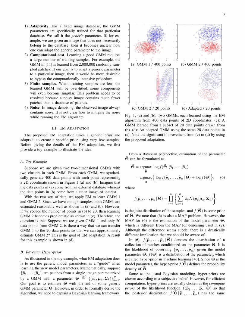
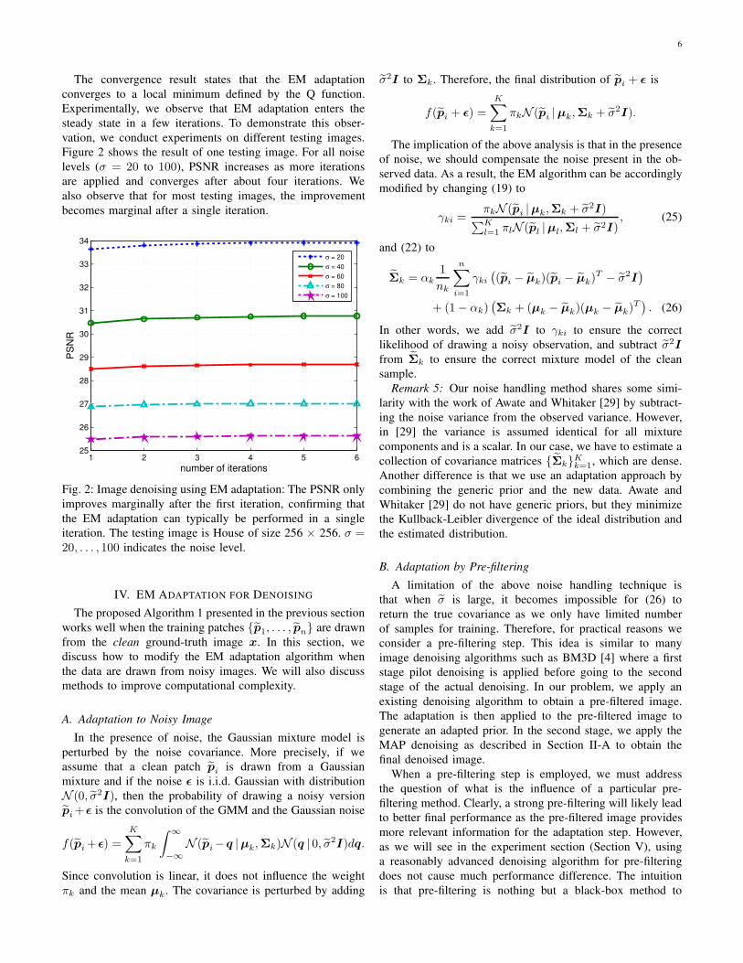
The convergence result states that the EM adaptation

converges to a local minimum defined by the Q function.

Experimentally, we observe that EM adaptation enters the

steady state in a few iterations. To demonstrate this obser-

vation, we conduct experiments on different testing images.

Figure 2 shows the result of one testing image. For all noise

levels (σ = 20 to 100), PSNR increases as more iterations

are applied and converges after about four iterations. We

also observe that for most testing images, the improvement

becomes marginal after a single iteration.

1 2 3 4 5 625

26

27

28

29

30

31

32

33

34

number of iterations

PS

NR

σ = 20

σ = 40

σ = 60

σ = 80

σ = 100

Fig. 2: Image denoising using EM adaptation: The PSNR only

improves marginally after the first iteration, confirming that

the EM adaptation can typically be performed in a single

iteration. The testing image is House of size 256 × 256. σ =20, . . . , 100 indicates the noise level.

IV. EM ADAPTATION FOR DENOISING

The proposed Algorithm 1 presented in the previous section

works well when the training patches {p̃1, . . . , p̃n} are drawn

from the clean ground-truth image x. In this section, we

discuss how to modify the EM adaptation algorithm when

the data are drawn from noisy images. We will also discuss

methods to improve computational complexity.

A. Adaptation to Noisy Image

In the presence of noise, the Gaussian mixture model is

perturbed by the noise covariance. More precisely, if we

assume that a clean patch p̃i is drawn from a Gaussian

mixture and if the noise ǫ is i.i.d. Gaussian with distribution

N (0, σ̃2I), then the probability of drawing a noisy version

p̃i+ǫ is the convolution of the GMM and the Gaussian noise

f(p̃i+ǫ) =

K∑

k=1

πk

∫ ∞

−∞

N (p̃i−q |µk,Σk)N (q | 0, σ̃2I)dq.

Since convolution is linear, it does not influence the weight

πk and the mean µk. The covariance is perturbed by adding

σ̃2I to Σk. Therefore, the final distribution of p̃i + ǫ is

f(p̃i + ǫ) =

K∑

k=1

πkN (p̃i |µk,Σk + σ̃2I).

The implication of the above analysis is that in the presence

of noise, we should compensate the noise present in the ob-

served data. As a result, the EM algorithm can be accordingly

modified by changing (19) to

γki =πkN (p̃i |µk,Σk + σ̃2I)

∑Kl=1 πlN (p̃l |µl,Σl + σ̃2I)

, (25)

and (22) to

Σ̃k = αk1

nk

n∑

i=1

γki((p̃i − µ̃k)(p̃i − µ̃k)

T − σ̃2I)

+ (1− αk)(Σk + (µk − µ̃k)(µk − µ̃k)

T). (26)

In other words, we add σ̃2I to γki to ensure the correct

likelihood of drawing a noisy observation, and subtract σ̃2I

from Σ̃k to ensure the correct mixture model of the clean

sample.

Remark 5: Our noise handling method shares some simi-

larity with the work of Awate and Whitaker [29] by subtract-

ing the noise variance from the observed variance. However,

in [29] the variance is assumed identical for all mixture

components and is a scalar. In our case, we have to estimate a

collection of covariance matrices {Σ̃k}Kk=1, which are dense.

Another difference is that we use an adaptation approach by

combining the generic prior and the new data. Awate and

Whitaker [29] do not have generic priors, but they minimize

the Kullback-Leibler divergence of the ideal distribution and

the estimated distribution.

B. Adaptation by Pre-filtering

A limitation of the above noise handling technique is

that when σ̃ is large, it becomes impossible for (26) to

return the true covariance as we only have limited number

of samples for training. Therefore, for practical reasons we

consider a pre-filtering step. This idea is similar to many

image denoising algorithms such as BM3D [4] where a first

stage pilot denoising is applied before going to the second

stage of the actual denoising. In our problem, we apply an

existing denoising algorithm to obtain a pre-filtered image.

The adaptation is then applied to the pre-filtered image to

generate an adapted prior. In the second stage, we apply the

MAP denoising as described in Section II-A to obtain the

final denoised image.

When a pre-filtering step is employed, we must address

the question of what is the influence of a particular pre-

filtering method. Clearly, a strong pre-filtering will likely lead

to better final performance as the pre-filtered image provides

more relevant information for the adaptation step. However,

as we will see in the experiment section (Section V), using

a reasonably advanced denoising algorithm for pre-filtering

does not cause much performance difference. The intuition

is that pre-filtering is nothing but a black-box method to

7

reduce the noise level σ̃. Since σ̃ can never be zero for any

pre-filtering method, we will have to use (25) and (26) by

replacing σ̃ with the amount of noise remaining in the pre-

filtered image. For most state-of-the-art denoising algorithms,

the difference in σ̃ is quite small. The real challenge is how

to estimate σ̃.

C. Estimating σ̃2

In order to analyze the noise remaining in the pre-filtered

image, we let x be the pre-filtered image. The distribution of

the residue x − x is unknown, but empirically we observe

that it can be approximated by a single Gaussian as in [45].

This approximation allows us to model (x−x) ∼ N (0, σ̃2I),

where σ̃2 def= E‖x−x‖2 is the variance of x. In other words,

σ̃2 is the mean squared error (MSE) of x compared to x.

Therefore, if x is available, estimating σ̃2 is trivial as it is just

the MSE. However, in the absence of x, we need a surrogate

to estimate the MSE and hence σ̃2.

The surrogate strategy we use is the Stein’s Unbiased Risk

Estimator (SURE) [46]. SURE provides a way for unbiased

estimation of the true MSE. The analytical expression of

SURE is

σ̃2 ≈ SUREdef=

1

n‖y − x‖2 − σ2 +

2σ2

ndiv, (27)

where div denotes the divergence of the denoising algorithm

with respect to the noisy measurements. However, not all

denoising algorithms have a closed form for the divergence

term. To alleviate this issue, we adopt the Monte-Carlo SURE

[47] to approximate the divergence. We refer readers to [47]

for detailed discussions about Monte-Carlo SURE. The key

steps are summarized in Algorithm 2.

Algorithm 2 Monte-Carlo SURE for Estimating σ̃2

Input: y ∈ Rn, σ2, δ (typically δ = 0.01).

Output: σ̃2.

Generate b ∼ N (0, I) ∈ Rn.

Construct y′ = y + δb.

Apply a denoising algorithm on y and y′ to get two pre-

filtered images x and x′, respectively.

Compute div = 1δb

T (x′ − x).

Compute σ̃2 = SUREdef= 1

n‖y − x‖2 − σ2 + 2σ2

n div.

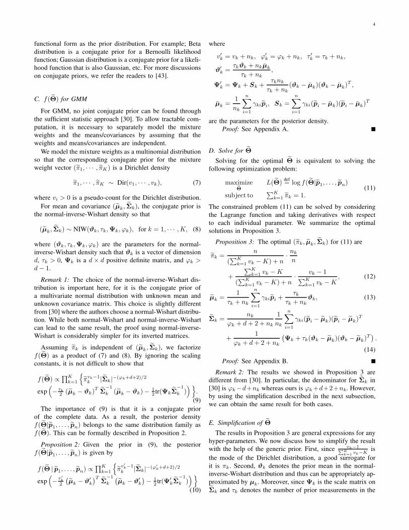
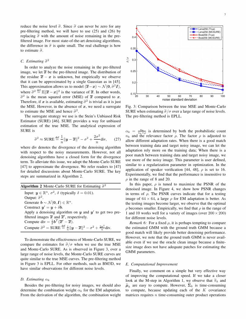
To demonstrate the effectiveness of Monte-Carlo SURE, we

compare the estimates for σ̃/σ when we use the true MSE

and Monte-Carlo SURE. As is observed in Figure 3, over a

large range of noise levels, the Monte-Carlo SURE curves are

quite similar to the true MSE curves. The pre-filtering method

in Figure 3 is EPLL. For other methods, such as BM3D, we

have similar observations for different noise levels.

D. Estimating αk

Besides the pre-filtering for noisy images, we should also

determine the combination weight αk for the EM adaptation.

From the derivation of the algorithm, the combination weight

20 30 40 50 60 70 80 90 1000.15

0.2

0.25

0.3

0.35

0.4

noise standard deviation

σ̃/σ

Lena256 (True)

Lena256 (MCSURE)

Boat256 (True)

Boat256 (MCSURE)

Fig. 3: Comparison between the true MSE and Monte-Carlo

SURE when estimating σ̃/σ over a large range of noise levels.

The pre-filtering method is EPLL.

αk = nk

nk+ρ is determined by both the probabilistic count

nk and the relevance factor ρ. The factor ρ is adjusted to

allow different adaptation rates. When there is a good match

between training data and target noisy image, we can let the

adaptation rely more on the training data; When there is a

poor match between training data and target noisy image, we

use more of the noisy image. This parameter is user defined,

similar to a regularization parameter in optimization. In the

application of speaker verification [44, 48], ρ is set to 16.

Experimentally, we find that the performance is insensitive to

ρ in the range of 8 and 20.

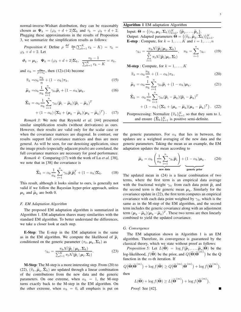
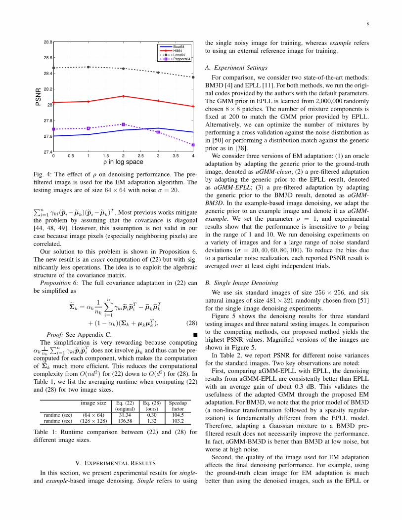
In this paper, ρ is tuned to maximize the PSNR of the

denoised image. In Figure 4, we show how PSNR changes

in terms of ρ. The PSNR curves indicate that for a testing

image of 64 × 64, a large ρ for EM adaptation is better. As

the testing images become larger, we observe that the optimal

ρ becomes smaller. Empirically, we find that ρ in the range of

1 and 10 works well for a variety of images (over 200× 200)

for different noise levels.

Remark 6: For a fixed ρ, it is perhaps tempting to compare

the estimated GMM with the ground truth GMM because a

good match will likely provide better denoising performance.

However, we note that the ground truth GMM is never avail-

able even if we use the oracle clean image because a finite-

size image does not have adequate patches for estimating the

GMM parameters.

E. Computational Improvement

Finally, we comment on a simple but very effective way

of improving the computational speed. If we take a closer

look at the M-step in Algorithm 1, we observe that π̃k and

µ̃k are easy to compute. However, Σ̃k is time-consuming

to compute, because updating each of the K covariance

matrices requires n time-consuming outer product operations

8

0 0.5 1 1.5 2 2.5 3 3.5 427.4

27.6

27.8

28

28.2

28.4

28.6

28.8

ρ in log space

PS

NR

Boat64Hill64Lena64Peppers64

Fig. 4: The effect of ρ on denoising performance. The pre-

filtered image is used for the EM adaptation algorithm. The

testing images are of size 64× 64 with noise σ = 20.

∑ni=1 γki(p̃i− µ̃k)(p̃i− µ̃k)

T . Most previous works mitigate

the problem by assuming that the covariance is diagonal

[44, 48, 49]. However, this assumption is not valid in our

case because image pixels (especially neighboring pixels) are

correlated.

Our solution to this problem is shown in Proposition 6.

The new result is an exact computation of (22) but with sig-

nificantly less operations. The idea is to exploit the algebraic

structure of the covariance matrix.

Proposition 6: The full covariance adaptation in (22) can

be simplified as

Σ̃k = αk1

nk

n∑

i=1

γkip̃ip̃Ti − µ̃kµ̃

Tk

+ (1− αk)(Σk + µkµTk ). (28)

Proof: See Appendix C.

The simplification is very rewarding because computing

αk1nk

∑ni=1 γkip̃ip̃

Ti does not involve µ̃k and thus can be pre-

computed for each component, which makes the computation

of Σ̃k much more efficient. This reduces the computational

complexity from O(nd2) for (22) down to O(d2) for (28). In

Table 1, we list the averaging runtime when computing (22)

and (28) for two image sizes.

image size Eq. (22) Eq. (28) Speedup(original) (ours) factor

runtime (sec) (64× 64) 31.34 0.30 104.5runtime (sec) (128× 128) 136.58 1.32 103.2

Table 1: Runtime comparison between (22) and (28) for

different image sizes.

V. EXPERIMENTAL RESULTS

In this section, we present experimental results for single-

and example-based image denoising. Single refers to using

the single noisy image for training, whereas example refers

to using an external reference image for training.

A. Experiment Settings

For comparison, we consider two state-of-the-art methods:

BM3D [4] and EPLL [11]. For both methods, we run the origi-

nal codes provided by the authors with the default parameters.

The GMM prior in EPLL is learned from 2,000,000 randomly

chosen 8× 8 patches. The number of mixture components is

fixed at 200 to match the GMM prior provided by EPLL.

Alternatively, we can optimize the number of mixtures by

performing a cross validation against the noise distribution as

in [50] or performing a distribution match against the generic

prior as in [38].

We consider three versions of EM adaptation: (1) an oracle

adaptation by adapting the generic prior to the ground-truth

image, denoted as aGMM-clean; (2) a pre-filtered adaptation

by adapting the generic prior to the EPLL result, denoted

as aGMM-EPLL; (3) a pre-filtered adaptation by adapting

the generic prior to the BM3D result, denoted as aGMM-

BM3D. In the example-based image denoising, we adapt the

generic prior to an example image and denote it as aGMM-

example. We set the parameter ρ = 1, and experimental

results show that the performance is insensitive to ρ being

in the range of 1 and 10. We run denoising experiments on

a variety of images and for a large range of noise standard

deviations (σ = 20, 40, 60, 80, 100). To reduce the bias due

to a particular noise realization, each reported PSNR result is

averaged over at least eight independent trials.

B. Single Image Denoising

We use six standard images of size 256 × 256, and six

natural images of size 481× 321 randomly chosen from [51]

for the single image denoising experiments.

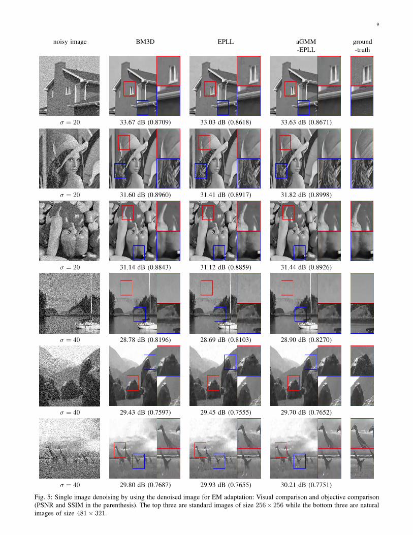
Figure 5 shows the denoising results for three standard

testing images and three natural testing images. In comparison

to the competing methods, our proposed method yields the

highest PSNR values. Magnified versions of the images are

shown in Figure 5.

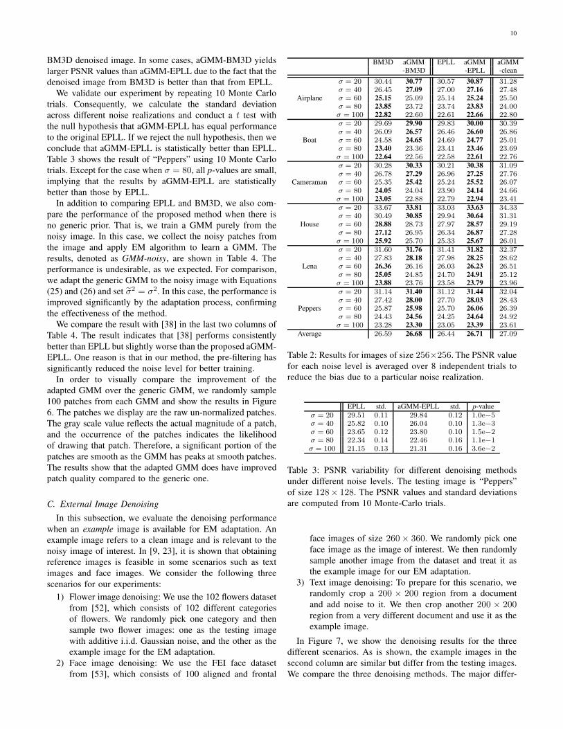
In Table 2, we report PSNR for different noise variances

for the standard images. Two key observations are noted:

First, comparing aGMM-EPLL with EPLL, the denoising

results from aGMM-EPLL are consistently better than EPLL

with an average gain of about 0.3 dB. This validates the

usefulness of the adapted GMM through the proposed EM

adaptation. For BM3D, we note that the prior model of BM3D

(a non-linear transformation followed by a sparsity regular-

ization) is fundamentally different from the EPLL model.

Therefore, adapting a Gaussian mixture to a BM3D pre-

filtered result does not necessarily improve the performance.

In fact, aGMM-BM3D is better than BM3D at low noise, but

worse at high noise.

Second, the quality of the image used for EM adaptation

affects the final denoising performance. For example, using

the ground-truth clean image for EM adaptation is much

better than using the denoised images, such as the EPLL or

9

noisy image BM3D EPLL aGMM ground

-EPLL -truth

σ = 20 33.67 dB (0.8709) 33.03 dB (0.8618) 33.63 dB (0.8671)

σ = 20 31.60 dB (0.8960) 31.41 dB (0.8917) 31.82 dB (0.8998)

σ = 20 31.14 dB (0.8843) 31.12 dB (0.8859) 31.44 dB (0.8926)

σ = 40 28.78 dB (0.8196) 28.69 dB (0.8103) 28.90 dB (0.8270)

σ = 40 29.43 dB (0.7597) 29.45 dB (0.7555) 29.70 dB (0.7652)

σ = 40 29.80 dB (0.7687) 29.93 dB (0.7655) 30.21 dB (0.7751)

Fig. 5: Single image denoising by using the denoised image for EM adaptation: Visual comparison and objective comparison

(PSNR and SSIM in the parenthesis). The top three are standard images of size 256× 256 while the bottom three are natural

images of size 481× 321.

10

BM3D denoised image. In some cases, aGMM-BM3D yields

larger PSNR values than aGMM-EPLL due to the fact that the

denoised image from BM3D is better than that from EPLL.

We validate our experiment by repeating 10 Monte Carlo

trials. Consequently, we calculate the standard deviation

across different noise realizations and conduct a t test with

the null hypothesis that aGMM-EPLL has equal performance

to the original EPLL. If we reject the null hypothesis, then we

conclude that aGMM-EPLL is statistically better than EPLL.

Table 3 shows the result of “Peppers” using 10 Monte Carlo

trials. Except for the case when σ = 80, all p-values are small,

implying that the results by aGMM-EPLL are statistically

better than those by EPLL.

In addition to comparing EPLL and BM3D, we also com-

pare the performance of the proposed method when there is

no generic prior. That is, we train a GMM purely from the

noisy image. In this case, we collect the noisy patches from

the image and apply EM algorithm to learn a GMM. The

results, denoted as GMM-noisy, are shown in Table 4. The

performance is undesirable, as we expected. For comparison,

we adapt the generic GMM to the noisy image with Equations

(25) and (26) and set σ̃2 = σ2. In this case, the performance is

improved significantly by the adaptation process, confirming

the effectiveness of the method.

We compare the result with [38] in the last two columns of

Table 4. The result indicates that [38] performs consistently

better than EPLL but slightly worse than the proposed aGMM-

EPLL. One reason is that in our method, the pre-filtering has

significantly reduced the noise level for better training.

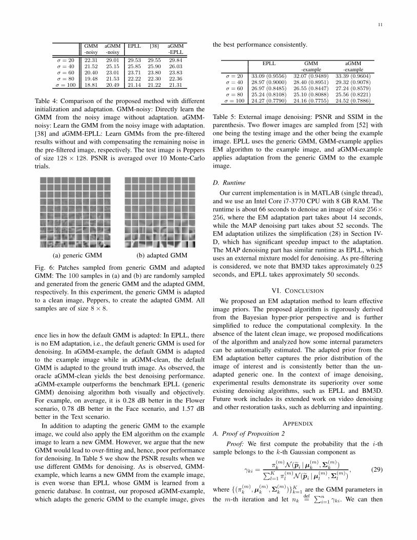
In order to visually compare the improvement of the

adapted GMM over the generic GMM, we randomly sample

100 patches from each GMM and show the results in Figure

6. The patches we display are the raw un-normalized patches.

The gray scale value reflects the actual magnitude of a patch,

and the occurrence of the patches indicates the likelihood

of drawing that patch. Therefore, a significant portion of the

patches are smooth as the GMM has peaks at smooth patches.

The results show that the adapted GMM does have improved

patch quality compared to the generic one.

C. External Image Denoising

In this subsection, we evaluate the denoising performance

when an example image is available for EM adaptation. An

example image refers to a clean image and is relevant to the

noisy image of interest. In [9, 23], it is shown that obtaining

reference images is feasible in some scenarios such as text

images and face images. We consider the following three

scenarios for our experiments:

1) Flower image denoising: We use the 102 flowers dataset

from [52], which consists of 102 different categories

of flowers. We randomly pick one category and then

sample two flower images: one as the testing image

with additive i.i.d. Gaussian noise, and the other as the

example image for the EM adaptation.

2) Face image denoising: We use the FEI face dataset

from [53], which consists of 100 aligned and frontal

BM3D aGMM EPLL aGMM aGMM-BM3D -EPLL -clean

Airplane

σ = 20 30.44 30.77 30.57 30.87 31.28σ = 40 26.45 27.09 27.00 27.16 27.48σ = 60 25.15 25.09 25.14 25.24 25.50σ = 80 23.85 23.72 23.74 23.83 24.00σ = 100 22.82 22.60 22.61 22.66 22.80

Boat

σ = 20 29.69 29.90 29.83 30.00 30.39σ = 40 26.09 26.57 26.46 26.60 26.86σ = 60 24.58 24.65 24.69 24.77 25.01σ = 80 23.40 23.36 23.41 23.46 23.69σ = 100 22.64 22.56 22.58 22.61 22.76

Cameraman

σ = 20 30.28 30.33 30.21 30.38 31.09σ = 40 26.78 27.29 26.96 27.25 27.76σ = 60 25.35 25.42 25.24 25.52 26.07σ = 80 24.05 24.04 23.90 24.14 24.66σ = 100 23.05 22.88 22.79 22.94 23.41

House

σ = 20 33.67 33.81 33.03 33.63 34.33σ = 40 30.49 30.85 29.94 30.64 31.31σ = 60 28.88 28.73 27.97 28.57 29.19σ = 80 27.12 26.95 26.34 26.87 27.28σ = 100 25.92 25.70 25.33 25.67 26.01

Lena

σ = 20 31.60 31.76 31.41 31.82 32.37σ = 40 27.83 28.18 27.98 28.25 28.62σ = 60 26.36 26.16 26.03 26.23 26.51σ = 80 25.05 24.85 24.70 24.91 25.12σ = 100 23.88 23.76 23.58 23.79 23.96

Peppers

σ = 20 31.14 31.40 31.12 31.44 32.04σ = 40 27.42 28.00 27.70 28.03 28.43σ = 60 25.87 25.98 25.70 26.06 26.39σ = 80 24.43 24.56 24.25 24.64 24.92σ = 100 23.28 23.30 23.05 23.39 23.61

Average 26.59 26.68 26.44 26.71 27.09

Table 2: Results for images of size 256×256. The PSNR value

for each noise level is averaged over 8 independent trials to

reduce the bias due to a particular noise realization.

EPLL std. aGMM-EPLL std. p-value

σ = 20 29.51 0.11 29.84 0.12 1.0e−5σ = 40 25.82 0.10 26.04 0.10 1.3e−3σ = 60 23.65 0.12 23.80 0.10 1.5e−2σ = 80 22.34 0.14 22.46 0.16 1.1e−1σ = 100 21.15 0.13 21.31 0.16 3.6e−2

Table 3: PSNR variability for different denoising methods

under different noise levels. The testing image is “Peppers”

of size 128× 128. The PSNR values and standard deviations

are computed from 10 Monte-Carlo trials.

face images of size 260× 360. We randomly pick one

face image as the image of interest. We then randomly

sample another image from the dataset and treat it as

the example image for our EM adaptation.

3) Text image denoising: To prepare for this scenario, we

randomly crop a 200 × 200 region from a document

and add noise to it. We then crop another 200 × 200region from a very different document and use it as the

example image.

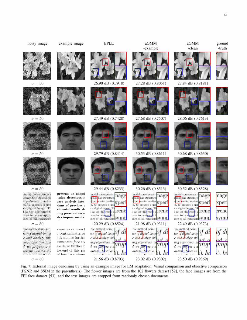
In Figure 7, we show the denoising results for the three

different scenarios. As is shown, the example images in the

second column are similar but differ from the testing images.

We compare the three denoising methods. The major differ-

11

GMM aGMM EPLL [38] aGMM-noisy -noisy -EPLL

σ = 20 22.31 29.01 29.53 29.55 29.84σ = 40 21.52 25.15 25.85 25.90 26.03σ = 60 20.40 23.01 23.71 23.80 23.83σ = 80 19.48 21.53 22.22 22.30 22.36σ = 100 18.81 20.49 21.14 21.22 21.31

Table 4: Comparison of the proposed method with different

initialization and adaptation. GMM-noisy: Directly learn the

GMM from the noisy image without adaptation. aGMM-

noisy: Learn the GMM from the noisy image with adaptation.

[38] and aGMM-EPLL: Learn GMMs from the pre-filtered

results without and with compensating the remaining noise in

the pre-filtered image, respectively. The test image is Peppers

of size 128 × 128. PSNR is averaged over 10 Monte-Carlo

trials.

(a) generic GMM (b) adapted GMM

Fig. 6: Patches sampled from generic GMM and adapted

GMM: The 100 samples in (a) and (b) are randomly sampled

and generated from the generic GMM and the adapted GMM,

respectively. In this experiment, the generic GMM is adapted

to a clean image, Peppers, to create the adapted GMM. All

samples are of size 8× 8.

ence lies in how the default GMM is adapted: In EPLL, there

is no EM adaptation, i.e., the default generic GMM is used for

denoising. In aGMM-example, the default GMM is adapted

to the example image while in aGMM-clean, the default

GMM is adapted to the ground truth image. As observed, the

oracle aGMM-clean yields the best denoising performance.

aGMM-example outperforms the benchmark EPLL (generic

GMM) denoising algorithm both visually and objectively.

For example, on average, it is 0.28 dB better in the Flower

scenario, 0.78 dB better in the Face scenario, and 1.57 dB

better in the Text scenario.

In addition to adapting the generic GMM to the example

image, we could also apply the EM algorithm on the example

image to learn a new GMM. However, we argue that the new

GMM would lead to over-fitting and, hence, poor performance

for denoising. In Table 5 we show the PSNR results when we

use different GMMs for denoising. As is observed, GMM-

example, which learns a new GMM from the example image,

is even worse than EPLL whose GMM is learned from a

generic database. In contrast, our proposed aGMM-example,

which adapts the generic GMM to the example image, gives

the best performance consistently.

EPLL GMM aGMM-example -example

σ = 20 33.09 (0.9556) 32.07 (0.9489) 33.39 (0.9604)σ = 40 28.97 (0.9000) 28.40 (0.8951) 29.32 (0.9078)σ = 60 26.97 (0.8485) 26.55 (0.8447) 27.24 (0.8579)σ = 80 25.24 (0.8108) 25.10 (0.8088) 25.56 (0.8221)σ = 100 24.27 (0.7790) 24.16 (0.7755) 24.52 (0.7886)

Table 5: External image denoising: PSNR and SSIM in the

parenthesis. Two flower images are sampled from [52] with

one being the testing image and the other being the example

image. EPLL uses the generic GMM, GMM-example applies

EM algorithm to the example image, and aGMM-example

applies adaptation from the generic GMM to the example

image.

D. Runtime

Our current implementation is in MATLAB (single thread),

and we use an Intel Core i7-3770 CPU with 8 GB RAM. The

runtime is about 66 seconds to denoise an image of size 256×256, where the EM adaptation part takes about 14 seconds,

while the MAP denoising part takes about 52 seconds. The

EM adaptation utilizes the simplification (28) in Section IV-

D, which has significant speedup impact to the adaptation.

The MAP denoising part has similar runtime as EPLL, which

uses an external mixture model for denoising. As pre-filtering

is considered, we note that BM3D takes approximately 0.25

seconds, and EPLL takes approximately 50 seconds.

VI. CONCLUSION

We proposed an EM adaptation method to learn effective

image priors. The proposed algorithm is rigorously derived

from the Bayesian hyper-prior perspective and is further

simplified to reduce the computational complexity. In the

absence of the latent clean image, we proposed modifications

of the algorithm and analyzed how some internal parameters

can be automatically estimated. The adapted prior from the

EM adaptation better captures the prior distribution of the

image of interest and is consistently better than the un-

adapted generic one. In the context of image denoising,

experimental results demonstrate its superiority over some

existing denoising algorithms, such as EPLL and BM3D.

Future work includes its extended work on video denoising

and other restoration tasks, such as deblurring and inpainting.

APPENDIX

A. Proof of Proposition 2

Proof: We first compute the probability that the i-thsample belongs to the k-th Gaussian component as

γki =π(m)k N (p̃i |µ

(m)k ,Σ

(m)k )

∑Kl=1 π

(m)l N (p̃i |µ

(m)l ,Σ

(m)l )

, (29)

where {(π(m)k ,µ

(m)k ,Σ

(m)k )}Kk=1 are the GMM parameters in

the m-th iteration and let nkdef=∑n

i=1 γki. We can then

12

noisy image example image EPLL aGMM aGMM ground

-example -clean -truth

σ = 50 26.90 dB (0.7918) 27.28 dB (0.8051) 27.84 dB (0.8181)

σ = 50 27.49 dB (0.7428) 27.68 dB (0.7507) 28.06 dB (0.7613)

σ = 50 29.79 dB (0.8414) 30.53 dB (0.8611) 30.68 dB (0.8630)

σ = 50 29.44 dB (0.8233) 30.26 dB (0.8513) 30.52 dB (0.8528)

σ = 50 20.29 dB (0.8524) 21.98 dB (0.9311) 22.49 dB (0.9373)

σ = 50 21.56 dB (0.8703) 23.02 dB (0.9302) 23.50 dB (0.9369)

Fig. 7: External image denoising by using an example image for EM adaptation: Visual comparison and objective comparison

(PSNR and SSIM in the parenthesis). The flower images are from the 102 flowers dataset [52], the face images are from the

FEI face dataset [53], and the text images are cropped from randomly chosen documents.

13

approximate log f(p̃1, . . . , p̃n)|Θ̃) in (6) by the Q function

as follows

Q(Θ̃|Θ̃(m)

) =n∑

i=1

K∑

k=1

γki log(π̃kN (p̃i|µ̃k, Σ̃k)

)

.=

n∑

i=1

K∑

k=1

γki

(log π̃k −

1

2log |Σ̃k|

−1

2(p̃i − µ̃k)

TΣ̃

−1

k (p̃i − µ̃k))

=

K∑

k=1

nk(log π̃k −1

2log |Σ̃k|)

−1

2

K∑

k=1

n∑

i=1

γki(p̃i − µ̃k)TΣ̃

−1

k (p̃i − µ̃k),

(30)

where.= indicates that some constant terms that are irrelevant

to the parameters Θ̃ are dropped.

We further define two notations

µ̄kdef=

1

nk

n∑

i=1

γkip̃i, Skdef=

n∑

i=1

γki(p̃i − µ̄k)(p̃i − µ̄k)T .

Using the equality

n∑

i=1

γki(p̃i − µ̃k)TΣ̃

−1

k (p̃i − µ̃k)

= nk(µ̃k − µ̄k)TΣ̃

−1

k (µ̃k − µ̄k) + tr(SkΣ̃−1

k ),

we can rewrite the Q function as follows

Q(Θ̃|Θ̃(m)

) =K∑

k=1

{nk(log π̃k −

1

2log |Σ̃k|)

−nk

2(µ̃k − µ̄k)

TΣ̃

−1

k (µ̃k − µ̄k)−1

2tr(SkΣ̃

−1

k )}.

Therefore, we have

f(Θ̃|p̃1, . . . , p̃n) ∝ exp(Q(Θ̃|Θ̃

(m)) + log f(Θ̃)

)

= f(Θ̃)

K∏

k=1

{π̃nk

k |Σ̃k|−nk/2

exp(−

nk

2(µ̃k − µ̄k)

TΣ̃

−1

k (µ̃k − µ̄k)−1

2tr(SkΣ̃

−1

k ))}

=

K∏

k=1

{π̃vk+nk−1k |Σ̃k|

−(ϕk+nk+d+2)/2exp(−

τk + nk

2

(µ̃k −τkϑk + nkµ̄k

τk + nk)T Σ̃

−1

k (µ̃k −τkϑk + nkµ̄k

τk + nk))

exp(−

1

2tr((Ψk + Sk

+τknk

τk + nk(ϑk − µ̄k)(ϑk − µ̄k)

T )Σ̃−1

k ))}

. (31)

Defining v′kdef= vk + nk, ϕ

′k

def= ϕk + nk, τ

′k

def= τk + nk,ϑ

′k

def=

τkϑk+nkµ̄k

τk+nk

, and Ψ′k

def= Ψk + Sk + τknk

τk+nk

(ϑk − µ̄k)(ϑk −

µ̄k)T , we will get

f(Θ̃|p̃1, . . . , p̃n) ∝∏K

k=1

{π̃v′

k−1

k |Σ̃k|−(ϕ′

k+d+2)/2

exp(−

τ ′

k

2

(µ̃k − ϑ′

k

)TΣ̃

−1

k

(µ̃k − ϑ′

k

)− 1

2 tr(Ψ′kΣ̃

−1

k ))}

,

which completes the proof.

B. Proof of Proposition 3

Proof: We ignore some irrelevant terms and get

log f(Θ̃|p̃1, . . . , p̃n).=

∑Kk=1{(v

′k − 1) log π̃k −

(ϕ′

k+d+2)2 log |Σ̃k| − τ ′

k

2 (µ̃k − ϑ′k)

TΣ̃

−1

k (µ̃k − ϑ′k) −

12 tr(Ψ′

kΣ̃−1

k )}. Taking derivatives with respect to π̃k, µ̃k and

Σ̃k will yield the following solutions.

• Solution to π̃k.

We form the Lagrangian

J(π̃k, λ) =

K∑

k=1

(v′k − 1) log π̃k + λ

(K∑

k=1

π̃k − 1

),

and the optimal solution satisfies

∂J

∂π̃k=

v′k − 1

π̃k+ λ = 0.

It is easy to see that λ = −∑K

k=1(v′k − 1), and thus the

solution to π̃k is

π̃k =v′k − 1

∑Kk=1(v

′k − 1)

=(vk − 1) + nk

(∑K

k=1 vk −K) + n

=n

(∑K

k=1 vk −K) + n·nk

n

+

∑Kk=1 vk −K

(∑K

k=1 vk −K) + n·

vk − 1∑K

k=1 vk −K. (32)

• Solution to µ̃k.

We let

∂L

∂µ̃k

= −τ ′k2Σ̃

−1

k (µ̃k − ϑ′k) = 0, (33)

of which the solution is

µ̃k =1

τk + nk

n∑

i=1

γkip̃i +τk

τk + nkϑk. (34)

• Solution to Σ̃k.

We let

∂L

∂Σ̃k

=−ϕ′k + d+ 2

2Σ̃

−1

k +1

2Σ̃

−1

k Ψ′kΣ̃

−1

k

+τ ′k2Σ̃

−1

k (µ̃k − ϑ′k)(µ̃k − ϑ′

k)TΣ̃

−1

k = 0,

which yields

(ϕ′k+d+2)Σ̃k = Ψ

′k+ τ ′k(µ̃k−ϑ

′k)(µ̃k−ϑ

′k)

T . (35)

14

Thus, the solution is

Σ̃k =Ψ

′k + τ ′k(µ̃k − ϑ′

k)(µ̃k − ϑ′k)

T

ϕ′k + d+ 2

=Ψk + τk(µ̃k − ϑk)(µ̃k − ϑk)

T

ϕk + d+ 2 + nk

+nk(µ̃k − µ̄k)(µ̃k − µ̄k)

T + Sk

ϕk + d+ 2 + nk

=nk

ϕk + d+ 2 + nk

1

nk

n∑

i=1

γki(p̃i − µ̃k)(p̃i − µ̃k)T

+1

ϕk + d+ 2 + nk

(Ψk + τk(ϑk − µ̃k)(ϑk − µ̃k)

T).

C. Proof of Proposition 6

Proof: We expand the first term in (22).

αk1

nk

n∑

i=1

γki(p̃i − µ̃k)(p̃i − µ̃k)T

= αk1

nk

n∑

i=1

γki(p̃ip̃Ti − p̃iµ̃

Tk − µ̃kp̃

Ti + µ̃kµ̃

Tk )

, αk1

nk

n∑

i=1

γkip̃ip̃Ti − (µ̃k − (1− αk)µk)µ̃

Tk

− µ̃k(µ̃k − (1 − αk)µk)T + αkµ̃kµ̃

Tk

= αk1

nk

n∑

i=1

γkip̃ip̃Ti − 2µ̃kµ̃

Tk

+ (1 − αk)(µkµ̃Tk + µ̃kµ

Tk ) + αkµ̃kµ̃

Tk , (36)

where , holds because αk1nk

∑ni=1 γkip̃i = µ̃k−(1−αk)µk

from (21). We then expand the second term in (22)

(1− αk)(Σk + (µk − µ̃k)(µk − µ̃k)

T)

= (1− αk)(Σk + µkµTk + µ̃kµ̃

Tk )

− (1− αk)(µkµ̃Tk + µ̃kµ

Tk ). (37)

Combining (36) and (37) completes the proof.

REFERENCES

[1] C. Tomasi and R. Manduchi, “Bilateral filtering for gray and colorimages,” in Proc. IEEE Intl. Conf. Computer Vision (ICCV’98), pp.839–846, 1998.

[2] A. Buades, B. Coll, and J. Morel, “A review of image denoisingalgorithms, with a new one,” SIAM Multiscale Model and Simulation,vol. 4, no. 2, pp. 490–530, 2005.

[3] C. Kervrann and J. Boulanger, “Local adaptivity to variable smoothnessfor exemplar-based image regularization and representation,” Intl. J.

Computer Vision, vol. 79, no. 1, pp. 45–69, 2008.[4] K. Dabov, A. Foi, V. Katkovnik, and K. Egiazarian, “Image denoising

by sparse 3D transform-domain collaborative filtering,” IEEE Trans.

Image Process., vol. 16, no. 8, pp. 2080–2095, Aug. 2007.[5] L. Zhang, W. Dong, D. Zhang, and G. Shi, “Two-stage image denoising

by principal component analysis with local pixel grouping,” Pattern

Recognition, vol. 43, pp. 1531–1549, Apr. 2010.[6] R. Yan, L. Shao, and Y. Liu, “Nonlocal hierarchical dictionary learning

using wavelets for image denoising,” IEEE Trans. Image Process., vol.22, no. 12, pp. 4689–4698, Dec. 2013.

[7] H. Takeda, S. Farsiu, and P. Milanfar, “Kernel regression for imageprocessing and reconstruction,” IEEE Trans. Image. Process., vol. 16,pp. 349–366, 2007.

[8] E. Luo, S. Pan, and T. Q. Nguyen, “Generalized non-local meansfor iterative denoising,” in Proc. 20th Euro. Signal Process. Conf.

(EUSIPCO’12), pp. 260–264, Aug. 2012.

[9] E. Luo, S. H. Chan, and T. Q. Nguyen, “Image denoising by targetedexternal databases,” in Proc. IEEE Intl. Conf. Acoustics, Speech and

Signal Process. (ICASSP ’14), pp. 2469–2473, May 2014.

[10] H. Talebi and P. Milanfar, “Global image denoising,” IEEE Trans.

Image Process., vol. 23, no. 2, pp. 755–768, Feb. 2014.

[11] D. Zoran and Y. Weiss, “From learning models of natural image patchesto whole image restoration,” in Proc. IEEE Intl. Conf. Computer Vision

(ICCV’11), pp. 479–486, Nov. 2011.

[12] M. Elad and M. Aharon, “Image denoising via sparse and redundantrepresentations over learned dictionaries,” IEEE Trans. Image Process.,vol. 15, no. 12, pp. 3736–3745, Dec. 2006.

[13] G. Yu, G. Sapiro, and S. Mallat, “Solving inverse problems with piece-wise linear estimators: From Gaussian mixture models to structuredsparsity,” IEEE Trans. Image Process., vol. 21, no. 5, pp. 2481–2499,May 2012.

[14] S. Roth and M. J. Black, “Fields of experts,” Intl. J. Computer Vision,vol. 82, no. 2, pp. 205–229, 2009.

[15] S. Roth and M. J. Black, “Fields of experts: A framework for learningimage priors,” in Proc. IEEE Conf. Computer Vision and Pattern

Recognition (CVPR’05), vol. 2, pp. 860–867, Jun. 2005.

[16] A. Buades, B. Coll, and J. M. Morel, “A non-local algorithm forimage denoising,” in IEEE Conference on Computer Vision and Pattern

Recognition (CVPR), vol. 2, pp. 60–65, 2005.

[17] S. P. Awate and R. T. Whitaker, “Higher-order image statistics forunsupervised, information-theoretic, adaptive, image filtering,” in IEEE

Conference on Computer Vision and Pattern Recognition (CVPR),vol. 2, pp. 44–51, 2005.

[18] P. Milanfar, “A tour of modern image filtering,” IEEE Signal Process.

Magazine, vol. 30, pp. 106–128, Jan. 2013.

[19] M. Zontak and M. Irani, “Internal statistics of a single natural image,” inProc. IEEE Conf. Computer Vision and Pattern Recognition (CVPR’11),pp. 977–984, Jun. 2011.

[20] I. Mosseri, M. Zontak, and M. Irani, “Combining the power ofinternal and external denoising,” in Proc. Intl. Conf. Computational

Photography (ICCP’13), pp. 1–9, Apr. 2013.

[21] H. C. Burger, C. J. Schuler, and S. Harmeling, “Learning how tocombine internal and external denoising methods,” Pattern Recognition,pp. 121–130, 2013.

[22] U. Schmidt and S. Roth, “Shrinkage fields for effective image restora-tion,” in Proc. IEEE Conf. Computer Vision and Pattern Recognition

(CVPR’14), pp. 2774–2781, Jun. 2014.

[23] E. Luo, S. H. Chan, and T. Q. Nguyen, “Adaptive image denoising bytargeted databases,” IEEE Trans. Image Process., vol. 24, no. 7, pp.2167–2181, Jul. 2015.

[24] H. Yue, X. Sun, J. Yang, and F. Wu, “CID: Combined image denoisingin spatial and frequency domains using web images,” in Proc. IEEE

Conf. Computer Vision and Pattern Recognition (CVPR’14), pp. 2933–2940, Jun. 2014.

[25] K. Tibell, H. Spies, and M. Borga, “Fast prototype based noisereduction,” in Image Analysis, pp. 159–168. Springer, 2009.

[26] F. Chen, L. Zhang, and H. Yu, “External patch prior guided internalclustering for image denoising,” in Proc. IEEE Intl. Conf. Computer

Vision (ICCV’15), pp. 603–611, Dec. 2015.

[27] S. P. Awate and R. T. Whitaker, “Nonparametric neighborhood statisticsfor mri denoising,” in Information Processing in Medical Imaging.Springer, pp. 677–688, 2005.

[28] S. P. Awate and R. T. Whitaker, “Unsupervised, information-theoretic,adaptive image filtering with applications to image restoration,” IEEE

Trans. Pattern Anal. Machine Intell., vol. 28, no. 3, pp. 364–376, 2006.

[29] S. P. Awate and R. T. Whitaker, “Feature-preserving MRI denoising:A nonparametric empirical Bayes approach,” IEEE Trans Medical

Imaging, vol. 26, no. 9, pp. 1242–1255, Sep. 2007.

[30] J. Gauvain and C. Lee, “Maximum a posteriori estimation for multi-variate Gaussian mixture observations of Markov chains,” IEEE Trans.

Speech and Audio Process., vol. 2, no. 2, pp. 291–298, Apr. 1994.

[31] T. Weissman, E. Ordentlich, G. Seroussi, S. Verdu, and M. J. Wein-berger, “Universal discrete denoising: Known channel,” IEEE Trans.

Information Theory, vol. 51, no. 1, pp. 5–28, Jan 2005.

15

[32] K. Sivaramakrishnan and T. Weissman, “A context quantization ap-proach to universal denoising,” IEEE Trans. Signal Process., vol. 57,no. 6, pp. 2110–2129, Jun 2009.

[33] A. Buades, B. Coll, and J. M. Morel, “Non-local means denoising,”[Available online] http://www.ipol.im/pub/art/2011/bcm nlm/, 2011.

[34] A. Levin and B. Nadler, “Natural image denoising: Optimality andinherent bounds,” in Proc. IEEE Conf. Computer Vision and Pattern

Recognition (CVPR’11), pp. 2833–2840, Jun. 2011.[35] A. Levin, B. Nadler, F. Durand, and W. T. Freeman, “Patch complexity,

finite pixel correlations and optimal denoising,” in Proc. 12th Euro.

Conf. Computer Vision (ECCV’12), vol. 7576, pp. 73–86. Oct. 2012.[36] S. H. Chan, T. Zickler, and Y. M. Lu, “Monte Carlo non-local means:

Random sampling for large-scale image filtering,” IEEE Trans. Image

Process., vol. 23, no. 8, pp. 3711–3725, Aug. 2014.[37] S. H. Chan, E. Luo, and T. Q. Nguyen, “Adaptive patch-based image

denoising by EM-adaptation,” in Proc. IEEE Global Conf. Signal and

Information Process. (GlobalSIP’15), Dec. 2015.[38] X. Lu, Z. Lin, H. Jin, J. Yang, and J. Z. Wang, “Image-specific prior

adaptation for denoising,” IEEE Trans. Image Process., vol. 24, no. 12,pp. 5469–5478, Dec. 2015.

[39] D. Geman and C. Yang, “Nonlinear image recovery with half-quadraticregularization,” IEEE Trans. Image Process., vol. 4, no. 7, pp. 932–946,Jul. 1995.

[40] D. Krishnan and R. Fergus, “Fast image deconvolution using hyper-Laplacian priors,” in Advances in Neural Information Process. Systems

22, pp. 1033–1041. Curran Associates, Inc., 2009.[41] C. A. Bouman, “Model-based image processing,” [Available online]

https://engineering.purdue.edu/∼bouman/publications/pdf/MBIP-book.pdf, 2015.

[42] M. R. Gupta and Y. Chen, Theory and Use of the EM Algorithm, NowPublishers Inc., 2011.

[43] C. M. Bishop, Pattern Recognition and Machine Learning, Springer,2006.

[44] D. A. Reynolds, T. F. Quatieri, and R. B. Dunn, “Speaker verificationusing adapted Gaussian mixture models,” Digital Signal Process., vol.10, no. 1, pp. 19–41, 2000.

[45] V. Papyan and M. Elad, “Multi-scale patch-based image restoration,”IEEE Trans. Image Process., vol. 25, no. 1, pp. 249–261, Jan. 2016.

[46] C. M. Stein, “Estimation of the mean of a multivariate normaldistribution,” The Annals of Statistics, vol. 9, pp. 1135–1151, 1981.

[47] S. Ramani, T. Blu, and M. Unser, “Monte-Carlo SURE: A black-box optimization of regularization parameters for general denoisingalgorithms,” IEEE Trans. Image Process., vol. 17, no. 9, pp. 1540–1554, Sep. 2008.

[48] P. C. Woodland, “Speaker adaptation for continuous density HMMs:A review,” in ITRW Adaptation Methods for Speech Recognition, pp.11–19, Aug. 2001.

[49] M. Dixit, N. Rasiwasia, and N. Vasconcelos, “Adapted Gaussian modelsfor image classification,” in Proc. IEEE Conf. Computer Vision and

Pattern Recognition (CVPR’11), pp. 937–943, Jun. 2011.[50] S. H. Chan, T. E. Zickler, and Y. M. Lu, “Demystifying symmetric

smoothing filters,” CoRR, vol. abs/1601.00088, 2016.[51] D. Martin, C. Fowlkes, D. Tal, and J. Malik, “A database of human

segmented natural images and its application to evaluating segmentationalgorithms and measuring ecological statistics,” in Proc. IEEE Intl.

Conf. Computer Vision (ICCV’01), vol. 2, pp. 416–423, 2001.[52] M. E. Nilsback and A. Zisserman, “Automated flower classification

over a large number of classes,” in Proc. Indian Conf. Computer Vision,

Graphics and Image Process. (ICVGIP’08), pp. 722–729, Dec. 2008.[53] C. E. Thomaz and G. A. Giraldi, “A new ranking method for principal

components analysis and its application to face image analysis,” Image

and Vision Computing, vol. 28, no. 6, pp. 902 – 913, 2010.

Enming Luo (S’14) received the B.Eng. degree inElectrical Engineering from Jilin University, China,in 2007, the M.Phil. degree in Electrical Engineer-ing from Hong Kong University of Science andTechnology in 2009 and the Ph.D. degree in Electri-cal and Computer Engineering at the University ofCalifornia, San Diego in 2016. He is now a researchscientist in Facebook.

Mr. Luo was an engineer at ASTRI, Hong Kong,from 2009 to 2010, and was an intern at Ciscoand InterDigital in 2011 and 2012, respectively. His

research interests include image restoration (denoising, super-resolution anddebluring), machine learning and computer vision.

Stanley H. Chan (S’06-M’12) received the B.Eng.degree in Electrical Engineering (with first classhonor) from the University of Hong Kong in 2007,the M.A. degree in Mathematics and the Ph.D.degree in Electrical Engineering from the Universityof California at San Diego, La Jolla, CA, in 2009and 2011, respectively.

Dr. Chan was a postdoctoral research fellow inthe School of Engineering and Applied Sciences andthe Department of Statistics at Harvard University,Cambridge, MA, from January 2012 to July 2014.

He joined Purdue University, West Lafayette, IN, in August 2014, where he iscurrently an assistant professor of Electrical and Computer Engineering, andan assistant professor of Statistics. His research interests include statisticalsignal processing and graph theory, with applications to imaging and networkanalysis. He was a recipient of the Croucher Foundation Scholarship for Ph.D.Studies 2008-2010 and the Croucher Foundation Fellowship for Post-doctoralResearch 2012-2013.

Truong Q. Nguyen (F’05) is currently a Professorat the ECE Dept., UCSD. His current researchinterests are 3D video processing and communi-cations and their efficient implementation. He isthe coauthor (with Prof. Gilbert Strang) of a popu-lar textbook, Wavelets & Filter Banks, Wellesley-Cambridge Press, 1997, and the author of sev-eral matlab-based toolboxes on image compression,electrocardiogram compression and filter bank de-sign.

Prof. Nguyen received the IEEE Transaction inSignal Processing Paper Award (Image and Multidimensional Processingarea) for the paper he co-wrote with Prof. P. P. Vaidyanathan on linear-phase perfect-reconstruction filter banks (1992). He received the NSF CareerAward in 1995 and is currently the Series Editor (Digital Signal Processing)for Academic Press. He served as Associate Editor for the IEEE Transactionon Signal Processing 1994-96, for the Signal Processing Letters 2001-2003,for the IEEE Transaction on Circuits & Systems from 1996-97, 2001-2004,and for the IEEE Transaction on Image Processing from 2004-2005.