VILNIUS UNIVERSITYFACULTY OF MATHEMATICS AND INFORMATICS

INSTITUTE OF COMPUTER SCIENCEDEPARTMENT OF COMPUTATIONAL AND DATA MODELING

Master Thesis

Hyperspectral Image Denoising

Done by:

Ignas Stočkus signature

Supervisor:dr. Valdas Rapševičius

Vilnius2020

Contents

Keywords and notations 3

Abstract 4

Santrauka 5

Introduction 6

1 Related Work and Theoretical Background 71.1 Hyperspectral images . . . . . . . . . . . . . . . . . . . . . . . . . . . . . . . . . 7

1.1.1 Hyperspectral imaging technology . . . . . . . . . . . . . . . . . . . . . . 71.1.2 Hyperspectral images data cubes . . . . . . . . . . . . . . . . . . . . . . . 7

1.2 Evaluating Noise in Hyperspectral Images . . . . . . . . . . . . . . . . . . . . . . 91.2.1 Noise origins . . . . . . . . . . . . . . . . . . . . . . . . . . . . . . . . . 91.2.2 Spatial and spectral correlation coefficients . . . . . . . . . . . . . . . . . 101.2.3 Linear regression based noise estimation algorithms . . . . . . . . . . . . 111.2.4 Image quality . . . . . . . . . . . . . . . . . . . . . . . . . . . . . . . . . 13

1.3 Denoising hyperspectral images . . . . . . . . . . . . . . . . . . . . . . . . . . . 131.3.1 Median filter . . . . . . . . . . . . . . . . . . . . . . . . . . . . . . . . . 131.3.2 Non-local means filtering . . . . . . . . . . . . . . . . . . . . . . . . . . 141.3.3 Wavelet transformation based image decomposition . . . . . . . . . . . . 151.3.4 Wavelet denoising . . . . . . . . . . . . . . . . . . . . . . . . . . . . . . 171.3.5 BM3D . . . . . . . . . . . . . . . . . . . . . . . . . . . . . . . . . . . . 19

2 Experimental Results 232.1 Hyperspectral Image Noise Evaluation . . . . . . . . . . . . . . . . . . . . . . . . 23

2.1.1 Experimental methods and data . . . . . . . . . . . . . . . . . . . . . . . 232.1.2 Correlation coefficients . . . . . . . . . . . . . . . . . . . . . . . . . . . . 242.1.3 Median filtering results . . . . . . . . . . . . . . . . . . . . . . . . . . . . 252.1.4 LMLSD and SSDC algorithms . . . . . . . . . . . . . . . . . . . . . . . . 272.1.5 Noise evaluation method comparisons . . . . . . . . . . . . . . . . . . . . 292.1.6 2D and 3D Wavelet based filtering . . . . . . . . . . . . . . . . . . . . . . 302.1.7 Block Matching 3D Filtering . . . . . . . . . . . . . . . . . . . . . . . . . 332.1.8 Image quality analysis . . . . . . . . . . . . . . . . . . . . . . . . . . . . 352.1.9 Filtering method comparison . . . . . . . . . . . . . . . . . . . . . . . . . 37

Conclusions and Recommendations 39

Future research work 40

References 41

2

Keywords and notations

HSI - Hyperspectral imageLM - Local meanLSD - Local noise standard deviationLMLSD - Local mean local noise standard deviationSSDC - Spatial spectral directBM3D - Block Matching 3DPSNR - Peak-Signal-To-Noise Ratio

3

Abstract

In this research paper we have analyzed hyperspectral images, hyperspectral imaging technolo-gies and the noise origins in hyperspectral images. We have analyzed and implemented multipleHSI noise evaluation methods: correlation coefficient based (R1 and R2) and linear regressionbased (LMLSD and SSDC). To compare different noise evaluation methods we have implementeda simple median filter as described in section 1.3.1. For the analysis we have used 5 differentnoisy hyperspectral crop images captured from an airborne drone. We have concluded that in allnoise evaluation methods the noise estimate parameter values were lower after filtering than in theoriginal image, therefore, concluding that our designed noise evaluation methodology can be usedto represent noise levels in HSI images. Furthermore, after analyzing the different noise evalua-tion methods we have concluded that the correlation coefficient based estimate methods and thelinear regression based methods all give different results on how effective the filtering is. Thiswas because the initial noise in the images was unknown, so we could not tell which of the noiseevaluation methods provided the most accurate representation of the noise. However, we havestill concluded that the linear regression based algorithm - LMLSD does not provide accurate re-sults in estimating the overall HSI data cube noise. The main reasons for the inaccurate resultswere identified as due to the noise not being fully homogeneous. However, the other implementedmethods - SSDC, R1 correlation coefficient and pixel correlation R2 provided with similar resultson determinig which are the most noisy bands and two of them were used to evaluate advancedfiltering algorithms. More advanced filtering algorithms were implemented and compared. Thebest results were given by the BM3D algorithm which outperformed wavelet 2D, 3D and the basicmedian filter in all noise estimate parameters. More importantly it did not change the originalsignal LM values and the initial signal remained intact after filtering (full results in table 7). Thiswas not demonstrated by any other method and this method is our recommendation for denoisingHSI images. Direct 2D and 3D Wavelet Transformation based filtering was, also, implementedwith different threshold functions and different wavelet forms. It was found that there are mini-mum dependencies on the selected wavelet form but big dependencies on thresholding functions.The best results were achieved with the λ threshold parameter and α threshold function (equations1.23, 1.22). 3D DWT based filtering performed worse compared to 2D due to images not havinghomogeneous noise in all bands and, therefore, impacting the thresholding parameter accuracy.As expected, median filtered provided good SSDC LSD results but it had the biggest changes insignal LM values, changing the original useful signal information. Finally, Peak-Signal-To-NoiseRatio (PSNR) parameter (equation 1.12) was calculated to asess image quality for different filter-ing technologies. The results showed that the worst performing method was the wavelet 3D. Othermethods provided simillar results with BM3D having the highest PSNR values in λε[550; 900]

inverval and lowest in λε[400; 550] and λε[900; 1000]. This means biggest filtering was done thelowest and highest bands, and least filtering was done in mid-range. Therefore, concluding thatthe BM3D targeted the noisiest channels for filtering leaving the least noisy intact.

4

Santrauka

Hiperspektrinių vaizdų triukšmo tyrimas

Šiame darbe analizavome hiperspektrinius vaizdus, hiperspektrinias vaizdavimo technologijasir triukšmo kilmę hiperspektriniuose vaizduose. Mes ištyrėme ir įgyvendinome kelis HSI triukšmovertinimo metodus: koreliacijos koeficientų suradimo metodikas (R1 ir R2) ir tiesinės regresijosmetodikas (LMLSD ir SSDC). Analizė atlikta su skirtingais hipersprektriniais vaizdais fotografuo-tais iš drono. Išnagrinėjus skirtingas triukšmo įvertinimo metodikas, padarėme išvadą, kad tiesinėsregresijos pagrindu sukurtas algoritmas LMLSD - neparodė gerų rezultatų įvertinant bendrą HSItriukšmą. Vis dėl to likusieji sukurti metodai: SSDC, koreliacijos koeficientų metodikos R1 ir R2

parodė adekvačius rezultatus ir jie gali būti naudojami įvertinant HSI triukšmus. Šie įvertinimometodai toliau buvo naudoti sukuriant ir lyginant skirtingas triukšmų šalinimo metodikas: BM3D,medianos filtro bei 2D ir 3D wavelet transformacijomis paremtomis metodikomis. Iš šių visųmetodų geriausiai pasirodė BM3D algoritmas, kuris sugebėjo ne tik labiausiai pašalinti triukšmusiš vaizdų bet ir mažiausiai iškraipė originalų signalą. Jis yra pateikiamas kaip mūsų rekomenduo-jamas metodas HSI triukšmų šalinimui įgyvendinti.

5

Introduction

One of the challenges of today’s agrarian culture is to be able to identify diseases of cultivatedplants early in their lifecycle [30]. Most often this is done by agronomists who manually examinethe crops seeking visual indicators that provide information about a possible disease. However,there are several issues with this verification method:

1. Large crop areas severely slow down this process as manual examination by the agronomistsbecomes nearly impossible.

2. The signs of the disease must be clearly visually visible. Visual signs usually only come upwhen the disease is already dominant in the crop and not in the first phase.

3. The diseases begin in very small local areas, so even in a full field manual check theagronomist might not find anything.

The ability to detect the disease early in its phase would allow farmers to take the necessary mea-sures to halt further progress which would reduce the financial damage suffered by farmers andreduce the amount of pesticides used in the treatment of illnesses and, therefore, reduce environ-mental pollution [23]. Because of these reasons there is interest in society and in the scientistscommunity on improving how to detect early signs of crop diseases. One of the suggested optionsis hyperspectral photography [25]. Hyperspectral images are obtained by flying with drones abovethe crop (rape, wheat, rye etc.) and filming them with portable hyperspectral cameras that cap-ture electromagnetic waves from 400 to 1000 nm in length. Specialized software then combinesthe obtained individual images and creates three-dimensional images (data cubes). These imagesare used for solving segmentation (classification) problems by classifying healthy crops and cropswith certain diseases. By comparing hyperspectral images which contain the same plants we cantell which of them are disease free and which of them have a distinct plant disease. However,before starting the classification these images must be preprocessed. As these captured images aremade by a flying drone in nature without any additional crop preparation or controlled ambientconditions they have a high noise level. This prevents further investigation and modeling of theresulting image. The noise levels can be very high on these images, therefore, modelling resultswithout any noise cancelling will be not be correct. Hence, one of the first and biggest challengesbecomes the identification and removal of noise in hyperspectral images [28]. Therefore, in thiswork, we will examine how to detect noise in hyperspectral images and how to distinguish thenoisy parts of the image from the noise free, and evaluate the magnitude of the noise. We will,also, try to apply denoising algorithms and compare how effective they were. We will try imple-ment already existing industry standard denoising methods and try determine which of them couldbe used to evaluate and remove noise in hyperspectral crop images.

Aim of the research – to investigate the noise reduction methods in hyperspectral images.Research tasks:

1. Create a noise in hyperspectral images evaluation methodology.

2. Implement hyperspectral image noise reduction methods and investigate the dependencieson noise reduction parameters.

3. Use the newly created noise evaluation methodology to compare different denoising algo-rithms and determine the most efficient one to use.

6

1 Related Work and Theoretical Background

1.1 Hyperspectral images

1.1.1 Hyperspectral imaging technology

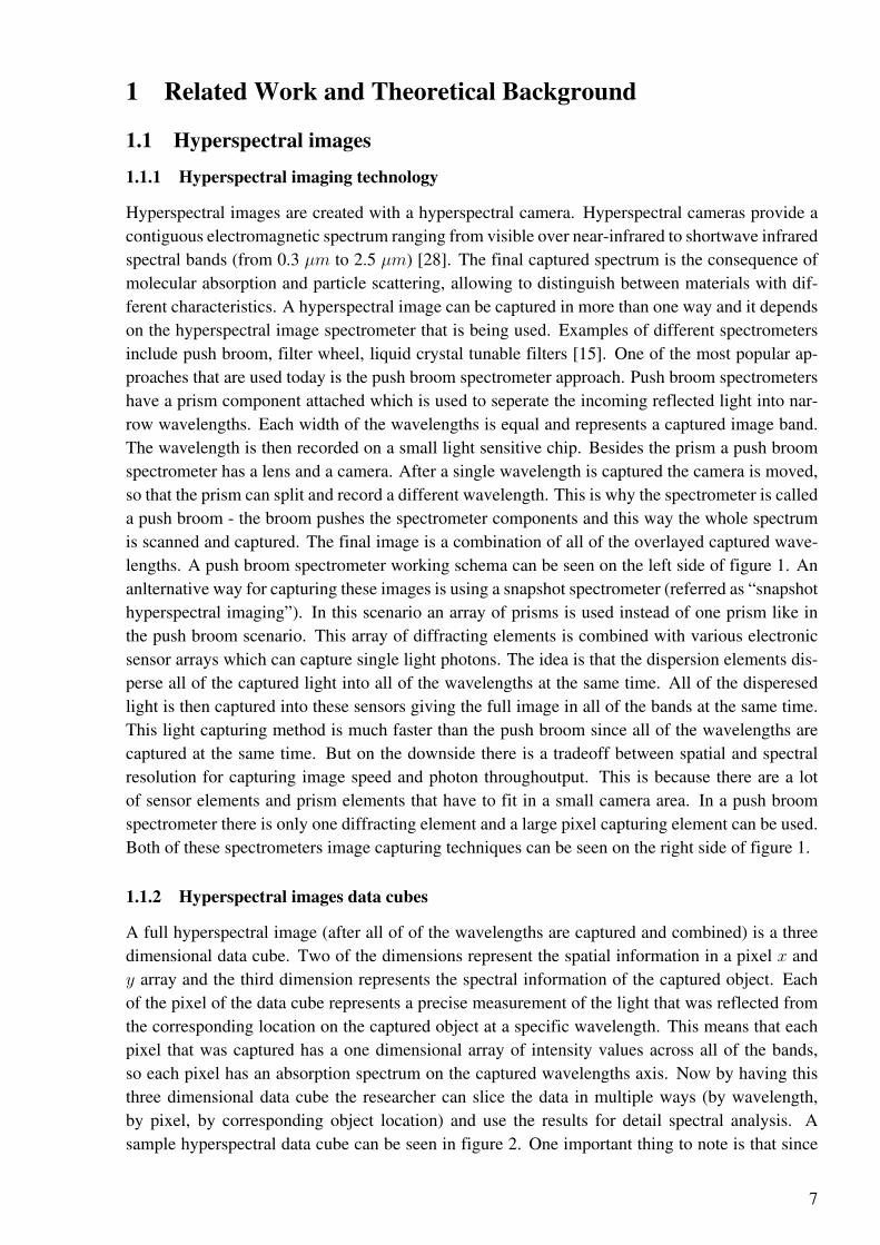
Hyperspectral images are created with a hyperspectral camera. Hyperspectral cameras provide acontiguous electromagnetic spectrum ranging from visible over near-infrared to shortwave infraredspectral bands (from 0.3 µm to 2.5 µm) [28]. The final captured spectrum is the consequence ofmolecular absorption and particle scattering, allowing to distinguish between materials with dif-ferent characteristics. A hyperspectral image can be captured in more than one way and it dependson the hyperspectral image spectrometer that is being used. Examples of different spectrometersinclude push broom, filter wheel, liquid crystal tunable filters [15]. One of the most popular ap-proaches that are used today is the push broom spectrometer approach. Push broom spectrometershave a prism component attached which is used to seperate the incoming reflected light into nar-row wavelengths. Each width of the wavelengths is equal and represents a captured image band.The wavelength is then recorded on a small light sensitive chip. Besides the prism a push broomspectrometer has a lens and a camera. After a single wavelength is captured the camera is moved,so that the prism can split and record a different wavelength. This is why the spectrometer is calleda push broom - the broom pushes the spectrometer components and this way the whole spectrumis scanned and captured. The final image is a combination of all of the overlayed captured wave-lengths. A push broom spectrometer working schema can be seen on the left side of figure 1. Ananlternative way for capturing these images is using a snapshot spectrometer (referred as “snapshothyperspectral imaging”). In this scenario an array of prisms is used instead of one prism like inthe push broom scenario. This array of diffracting elements is combined with various electronicsensor arrays which can capture single light photons. The idea is that the dispersion elements dis-perse all of the captured light into all of the wavelengths at the same time. All of the disperesedlight is then captured into these sensors giving the full image in all of the bands at the same time.This light capturing method is much faster than the push broom since all of the wavelengths arecaptured at the same time. But on the downside there is a tradeoff between spatial and spectralresolution for capturing image speed and photon throughoutput. This is because there are a lotof sensor elements and prism elements that have to fit in a small camera area. In a push broomspectrometer there is only one diffracting element and a large pixel capturing element can be used.Both of these spectrometers image capturing techniques can be seen on the right side of figure 1.

1.1.2 Hyperspectral images data cubes

A full hyperspectral image (after all of of the wavelengths are captured and combined) is a threedimensional data cube. Two of the dimensions represent the spatial information in a pixel x andy array and the third dimension represents the spectral information of the captured object. Eachof the pixel of the data cube represents a precise measurement of the light that was reflected fromthe corresponding location on the captured object at a specific wavelength. This means that eachpixel that was captured has a one dimensional array of intensity values across all of the bands,so each pixel has an absorption spectrum on the captured wavelengths axis. Now by having thisthree dimensional data cube the researcher can slice the data in multiple ways (by wavelength,by pixel, by corresponding object location) and use the results for detail spectral analysis. Asample hyperspectral data cube can be seen in figure 2. One important thing to note is that since

7

,

Figure 1. Main push broom spectrometer components (left figure) [20]. Two of the most popularhyperspectral images capturing techniques: push broom (right figure A) and snapshot (right figureB) [33]. Push broom - the broom pushes each filter to capture a single wavelength at a time.Snapshot - an array of dispersion elements disperses the captured wavelengths to seperate sensorsfor a full captured image at all wavelengths.

each spectral band is very narrow (only a few nm), the captured signal for that wavelength isalso very weak. This means there is a trade-off between spatial and spectral resolution for theimage. Therefore, to increase the resolution hyperspectral images are taken airborne (attaching ahyperspectral camera to a drone or low a flying plane, or other machine). This ensures that morelight for each wavelength is being captured and the images have higher spectral resolution.

One more important factor to consider when analyzing a hyperspectral image data is the datasize. HSI by default is large in size. For example a scan of a single plant could easily be arounda gigabyte in size [23]. For example, during this research the file sizes were ranging from 250megabytes to 700 megabytes. If we want to analyze the whole spectrum of such images it will takeconsiderably longer for the processing to take than compared to smaller files. An easy solution forthis is to not use all of data from all the bands. For example, if we have captured 800 differentbands we can only use 400 bands by combining the bands into bigger bins where each bin isthe same size and contains information from multiple bands. However, when using only part ofthe data the researcher might miss some valuable information that was present only in specificwavelengths and the analysis of the image might not be deep enough. A different approach isto use only the wavelengths that the researcher is interested in. If we know exactly what we arelooking for in the images (which disease signs are dominant in which band) we can only look intothe bands that we are interested in. However, this approach requires additional knowledge of theimage background and does not work for preventive scanning tasks. In conclusion, the researchershould consider all of the factors for the data analysis task and decide whether to use all of the datafor a more detail analysis and sacrifice speed, or it is enough to combine multiple bands leavingout some information during compression for a more faster analysis (when there are a lot of imagesto process).

8

,

Figure 2. A sample hyperspectral image three dimensional data cube schema (left) and a samplereflectance spectra whithin one pixel (right) [15].

1.2 Evaluating Noise in Hyperspectral Images

1.2.1 Noise origins

Since the main object of the study is noise, the following will discuss what the main types of noiseare found in hyperspectral images. A noisy image can be defined as [18]:

g(x, y) = f(x, y) + n(x, y) (1.1)

where x, y - pixel coordinates in the pixel plane of the image, f(x, y) - signal pixel intensitywithout the noise (clean image where Signal-To-Noise ratio would be 1) and n(x, y) - the intensityof noise of pixel at cordinates x, y.

This means that the total signal itensity of each pixel is determined by the actual intensity ofthe collected light and the noise factor existing in the channel. Depending on the type of noisethe factor n(x, y) varies. There are 3 most common types of noise that are found in hyperspectralimages [32]:

1. Impulse noise

2. Gaussian noise

3. Periodic noise

Firstly, let us briefly discuss the impulse noise. The defining characteristic of this noise is thatit is defined by a random distribution of placement and intensity of the noise. For impulse noisethe noise component n(x, y) will have random black or white pixel intensity values. This meansthat this noise causation are all the external factors affecting the signal when the images are taken.In a scenaraio where a drone is flying and filming crops this noise can be caused by various factorssuch as: the wind and drone vibrations during imaging, varying weather conditions, existence ofsolid particles in the air dispersing reflected light, varying density of crops on the ground, varyingterrain causing difference in reflection and others. This noise usually is the dominant type of noisein hyperspectral images and it is the hardest one to account for. Next, we have Gaussian noise.This noise is not accidental and not random - this noise follows the Gaussian dependency and

9

follows the normal distribution. The probability density function p of a Gaussian noise variable zis given by [7]:

pG(z) =1

σ√

2πe−

(z−µ)2

2σ2 (1.2)

where z represents the grey level, µ the mean value and σ the standard deviation [7].This noise is often caused by electronic and optical imperfections: sensor inaccuracies, im-

perfect optics of the camera lens, noise of the electronic circuits. Also, this can be sensor noisecaused by poor illumination and/or high temperature, and/or transmission. In digital image pro-cessing Gaussian noise can be reduced by using a spatial filter but when attempting such procedurean undesirable outcome may result in the blurring of the image edges and details. This is becausethey usually correspond to the blocked high frequencies. Conventional spatial filtering techniquesfor noise removal include: mean filtering, median filtering and Gaussian smoothing [3]. Lastly,we have the periodic noise which is characterized by its periodic repetition in the image, so it canbe described as as a periodic function [18]:

n(x, y) = Asin(Uox+ Voy) (1.3)

where A is the amplitude of noise intensity, Uo and Vo - noise frequency components.A common source of periodic noise in an image is from electrical or electromechanical inter-

ference during the image capturing process [17]. An image affected by periodic noise will looklike a repeating pattern has been added on top of the original image. In the frequency domain thistype of noise can be seen as discrete spikes. Significant reduction of this noise can be achieved byapplying notch filters in the frequency domain [17].

1.2.2 Spatial and spectral correlation coefficients

In order to estimate the magnitude of noise in hyperspectral images we will calculate the correlationcoefficients between two adjacent noisy channels e.g between two adjacent wavelengths. Wewill, also, calculate the correlation coefficients for each image pixel and their neighboring pixelsbetweeen all image bands (all wavelengths). The correlation coefficient between close bands R1

will be defined as [32]:

R1 =

∑Mm=1

∑Nn=1(Amn − A)(Bmn −B)√

(∑M

m=1

∑Nn=1(Amn − A)2)

√(∑M

m=1

∑Nn=1(Bmn −B)2)

(1.4)

where M and N are the pixel matrixes of the same dimension of the neighboring bands that R1 iscalculated, and A and B are the mean values of the of A and B.

Next, we will also find the correlation of each pixel intensity values and its neighboring pixelvalues between all the bands. The calculation of the correlation coefficient between two neighbor-ing pixel intensity values on all the bands will be defined from the Pearson correlation coefficientas:

R2i =

∑Ni=1(Y1i − Y1)(Y2i − Y2)√∑N

i=1(Y1i − Y1)2

√∑Ni=1(Y2i − Y2)2

(1.5)

where N is the total number of all of the bands, Y1i is the pixel at location Amn intensity value,Y2i is one of the neighboring pixel at location Am+−1n+−1 intensity values, and, Y1 and Y2 are the

10

means of intensities of the center pixel and one of neighboring pixels across all of the bands. Thetotal correlation coefficient for the pixel will be the average across all of the correlation coefficientscalculated for that pixel and its neighbors.

R2 =

∑8i=1R2i

N(1.6)

These correlation factors will help us to evaluate the noisiest channels and the noisiest pixels.This methodology is based on the fact that the existing noise in the images does not correlate wellbetween bands such as the main signal does. Signal intensity correlates well between adjacentchannels and between adjacent pixels. That means that the correlation coefficients R1 betweenclose bands and R2 for all pixels in the same band should be very simmalar to other bands/pixels.Therefore, if there is relatively much noise existing in some channels, adjacent channels R1 valueswill be low and the noise component n(x, y) will be much larger than in the noise free channels.The same can be applied to the pixels, the same pixel intensity values in all the wavelengths shouldhave a high correlation coefficient between other neighboring pixels. That means the pixels whichwill have the lowest correlation coefficients R2 values will be the most noisy ones and their noisecomponent n(x, y) will be much larger than in the other noise free pixels. After having determinedthe noisiest channels and pixels the next step would be to apply noise reduction methods for thenoisiest channels/pixels and calculate the correlation coefficients again to evaluate the results.

1.2.3 Linear regression based noise estimation algorithms

Besides calculation of the corellation coefficients another type of methods can be used. These typeof methods use linear regression based models to evaluate the noise in each seperate band and theyalso give a noise estimate for the entire image. The correlation coefficient method was not capableof estimating the whole hyperspectral image. We will examine and later experimentally test twolinear reggression based methods: LMLSD (Local Mean Local Noise Standard Deviation) andSSDC (Spatial Spectral Direct Corellation). Both of these algorihtms were developed in the 1990’sand both of these algorithms have also been improved since they were initially created. The newversions of these algorithms are called the RLSD and HRDSDC. First of all, we will understandand test out the original versions, so using the newer one is out of scope of this research. Firstly,let us examine the LMLSD algorithm. This method assumes that the whole hyperspectral image ismade up of many homogeneous blocks. This means that the photographed image should containthe same photographed objects, materials, substances etc. Having different materials in the imagewould drastically reduce the accuracy of this method. The first step is to divide the entire imageinto non-overlapping blocks where in each block we would have w ∗ w pixels (w - block spatialdimension). The LMLSD only takes into account the spatial correlations of pixels in each bandwithout the spectral correlations. This means that the blocks are 2D and each will contain w ∗ wnumber of pixels in each band. Also, each band will have the same number of blocks, since eachband has the same spatial dimensions. Now the local mean (LM) of the signal in each band can becalculated as [16]:

LM =1

w2

w∑i=1

w∑j=1

xi,j,k (1.7)

where w is the block dimension, xi,j,k - pixel value in band k. Now it is assumed that the deviationfrom this local mean (LM) is due to noise, therefore, the noise is estimated by the local noise

11

standard deviation (LSD) and is estimated for each block as [16]:

LSD =

√√√√ 1

w2 − 1

w∑i=1

w∑j=1

(xi,j,k − LM)2 (1.8)

where LSD is considered to be as the noise standard deviation of the block in band k and LM isthe signal mean for that block.

When each block has the LSD parameter calculated the minimum and maximum values ofthe standard deviations are found. In this interval bins of equal width are created. The numbercan be from 1 (the mean value of standard deviation) up to N depending on the images nature.The number of blocks falling into each bin are counted and the bin with the highest number ofblocks is going to represent the noise standard deviation for the entire image independent of bandsnoise deviations. The actual noise standard deviation mean value in the bin is considered as theestimated noise of the HSI [16]. Depending on the number of bins the results will vary. If thehyperspectral image is not homogeneous than the estimated noise value can vary a lot from themean of standard deviation. Also, if the number of bins is too high than the differences betweenthe means in neighboring bins can be very small. This means that an expected interval to representthe image noise standard deviation is going to be split into multiple ones with small differences.Now the largest bin can become any other bin which has a few more LSD block values and it willbe incorrectly considered as the noise estimate for the image.

An alternative method which solves the previously mentioned problem is the SSDC algorithmmethod. This method is more advanced than the first one since it uses spectral (between band) andspatial (within band) correlations. This method uses these correlations to de-correlate the imagedata with linear reggression. The estimated noise is assumed to be the unexplained residualsbetween the real values and the modeled values with linear reggression. As with the LMLSDmethod the image is divided into w ∗ w blocks in each band. Each pixel in the block at (i, j)

coordinates in band k can be predicted by the pixels spatial and spectral neighbors. Now theresidual is calculated as [16]:

ri,j,k = xi,j,k − ˆxi,j,k (1.9)

where ˆxi,j,k is the predicted value of xi,j,k with linear reggression and ˆxi,j,k is computed as [16]:

ˆxi,j,k = a+ bxi,j,k−1 + cxi,j,k+1 + dxp,k (1.10)

where p expresses the spatial adjacent pixels of xi,j,k and a, b, c, d are the coefficients determinedby multiple linear reggression. The same noise standard deviation LSD of a block can be calculatedas the sum of all residuals in the block and would be equal to [16]:

LSD =

√√√√ 1

w2 − 4

w∑i=1

w∑j=1

r2i,j,k (1.11)

where the mean value of all the blocks in band k is considered as the band noise estimate value.For the whole image - the mean value of all LSD values. In this formal equation 1.10 for LSDcalculation only one band above (k + 1), one band below (k − 1) and one spatial neighbor formultiple linear reggression is used. However, the p can be extended for up to 8 adjacent pixelneighbors for more precise calculations, since correlation must exist between all pixels in the same

12

band. If more neighbors of xi,j,k are going to be used than more coefficients in the multiple linearreggression have to be determined. At first glance this method is better than the LMLSD approach,since it also includes spectral bands which also have correlation with the signal between bands.Also, it solves the bin problem as discussed above for images that are not homogeneous. We willtest these methods experimentally.

1.2.4 Image quality

Previously mentioned models can be implemented to determine and evalute noise in a HSI image.However, we do not have a parameter which would compare different filtering techniques by theoverall image quality. Visual comparisons are not possible due to the nature of HSI data (data iscaptured and combined into data cubes from multiple wavelengths). For example, median filteringcan be very effective in removing noise as determined by our methods but a lot of useful informa-tion during median filtering is, also, lost. This is why there is a need for more advanced techniques.Therefore, we will introduce another parameter to compare different filtering techniques. This pa-rameter will be Peak Signal-To-Noise ratio or PSNR. PSNR is most commonly used to measurethe quality of reconstruction of lossy compression codecs (e.g., for image compression) and, also,in comparing digital image filtering methods. Also, it is commonly found on similar research workin HSI. PSNR is defined in dB as [29]:

PSNR = 10log10(max2(x)

MSE(x, x)) (1.12)

where x is a vectorized clean image of length N , x is the vectorized denoised image and MSE(Mean Squared Error) is defined as:

MSE(x, x) =1

N

N−1∑i=0

(x(i)− ˙x(i)))2 (1.13)

The only issue with the above definition is that in our research we do not have a clean imagebaseline as the images are captured from real world scenarios. This means we will have to comparethe noisy image and the denoised image. In this case we will still get good sense of the imagequality for filtering techniques comparisons (as the baseline is the same) but the exact PSNR valuescould not be used in giving exact measureable values as we are calculating MSE with noise whichbrings extra devations. To perform an exact, measureable filtering image quality comparisons wewould need to use a noisy free image, introduce artificial noise to it and then denoise it with all thetechniques. However, this can be done in an extension of this work as the goal is to try to find thebest denoising technique for real world HSI images with noise.

1.3 Denoising hyperspectral images

1.3.1 Median filter

The first technique that is going to be used for denoising hyperspectral images is a median filter.This approach is widely used in normal 2D pixel images noise reduction and it can also be appliedto a hyperspectral data cube. In a data cube the median filter must be applied to each wavelength ina x and y pixel array. This will reduce the salt and pepper noise (impulse noise) in that wavelength.After applying the filter we can construct a new datacube with the same spatial dimensions. The

13

spectral dimension values will contain the new denoised, median values after the filtering. Themedian filter considers each pixel in the data cube band one by one and looks at its nearby neigh-bors to decide whether it is representative of its surroundings. Then it replaces the center pixelvalue with the median of those neighboring values. The median is calculated by first sorting all thepixel values from the surrounding neighborhood into numerical order and then replacing the centerpixel with the middle pixel value. We will be implementing a 3 x 3 median filter. This means wewill consider only the closest neighboring pixel values (in the general case - 8 neighboring pixelvalues) in the median calculation. We will be using the median filter to measure the noises levelsof our hyperspectral images and to test out our noise evaluation methods as defined previously.After having analyzed if our evaluation methods work we will use the results to evaluate moreadvanced filtering techniques which will be discussed next.

1.3.2 Non-local means filtering

While the previously described median filter would be effective in denoising the HSI cube, it isalso effective in clearing out the signal values, therefore, loosing information and details. In imagedenoising there are other, more advanced algorithms that are used. One of the most popular one isthe non-local means denoising algorithm. Unlike local mean filter, which takes the mean value ofa group of pixels surrounding a target pixel to smooth the image, non-local means filtering takes amean of all pixels in the image, weighted by how similar these pixels are to the target pixel. Thisresults in much greater post-filtering clarity, and less loss of detail in the image compared withlocal mean algorithms [4]. With this approach a band pixel array would be divided into patchesor blocks of w ∗ w pixels. A scan of the entire band would begin to search for similar patchesas the current one. After the search is completed denoising would take place. Denoising is doneby computing the average pixel values of these most resembling pixels. For a formal mathemicalequation the filtering can be defined as [6]:

u(p) =1

C(p)

∫Ω

v(q)f(p, q)dq (1.14)

where Ω is the area of the pixel array in band k, p and q are the two points within the imageband. In a patch scenario these would be two distinct patches in size w ∗ w. The filtered value atthe location p would be u(p). V (q) is the unfiltered value of the image in location q and f(p, q)

would be the weighting function based on the pixel patch distance and similarities. C(p) is thenormalizing factor given by:

C(p) =

∫Ω

f(p, q)dq (1.15)

The purpose of the weighting function is to determine how closely related the image patches (pix-els) are in the locations p and q and it can take various forms. The most used one is the Gaussianweighting function which sets up a normal distribution of noise with a mean and a standard devia-tion. This form assumes that the noise found in the image follows the normal distribution arroundthe signal mean values. Since in our HSI images the noise origin and variance is unknown it issafe to assume that this noise type should be accounted for. When the noise origins are known amore precise weighting function can be used. In our case we will be using the Gaussian weightingfunction, which is defined as [5]:

f(p, q) = e−|B(q)−B(p)|2

h2 (1.16)

14

where h is the filtering factor (standard deviation of signal in the image or i.e noise) and B(p) isthe local mean value of the image surrounding the point p. In a real implementation some cornercutting must be made. For example, the search for similar pixels. The search would need be in alocal neighborhood and not in the entire band as described with the integral of Ω (search size isfound to be up to 35 * 35 neighboring pixels in some sources). This is because a search throughentire band for each of the pixel patch would take a very long time to complete, especially, for aHSI data cube with 200 bands. Still as compared to the local median filtering where only the 1x 1 neighbors are considered and without weight function, this filtering would provide with moreprecise results and with less lost information. Next, we will look at some examples of the non-localfiltering techniques - BM3D and BM4D filtering methods. These will be discussed after wavelettransformation based filtering and thresholding methods since both of these concepts are found inBM3D and BM4D.

1.3.3 Wavelet transformation based image decomposition

Another common hyperspectral image filtering technique is by using 2D and 3D wavelet transfor-mations. This approach combines the wavelet transformations with thresholding. Wavelet analysisis considered a state-of-the-art technique in signal processing; it transforms the signal into a scale-time representation (scalogram) with high resolution, preserving the temporal characteristics ofthe signal. It has a key advantage compared to another popular spectral analysis approach - theFourier transformations. It captures both frequency and location (location in time) information.Wavelets emerged in the 1960’s allowing to represent signal both in time and frequency domainsimultaneously. This way, not only both time and frequency information is available, it is alsopossible to store signal efficiently [12]. Mathematically, wavelets are nothing but functions thatdivide the original signal into different frequency components and study each component. Thebasis functions of Wavelet Transform (WT) are scaled according to the frequency. There are dif-ferent small waves (also known as mother wavelets) that can be used for the implementation ofWT [9]. Some most popular forms of wavelets include Dubachies, Haar, Symlet, Coiflet, MexicanHat, Morlet. Some of these wavelet forms can be seen in figure 3. Each of them comes fromdifferent wavelet families and includes different properties [9]. We decide which wavelet to applyin different cases and scenarios depending on the requirements of the application. There are twotypes of WT defined as Continues Wavelet Transform (CWT) and Discrete Wavelet Transform(DWT). In the CWT, the analyzing function is a wavelet ψ. The CWT compares the signal toshifted and compressed or stretched versions of a wavelet. Stretching or compressing a function iscollectively referred to as dilation or scaling and corresponds to the physical notion of scale. Bycomparing the signal to the wavelet at various scales and positions, you obtain a function of twovariables [1]. The common form for CWT can be written as:

C(a, b; f(t), ψ(t)) =

∫ ∞−∞

f(t)1

aψ∗(

t− ba

)dt (1.17)

where ψ∗ denotes the complex conjugate of the analysing function (wavelet), f(t) is the originalsignal, a is a scale parameter and b is a position in time. By continuously varying the values of thescale parameter, a, and the position parameter, b, you obtain the CWT coefficients C(a, b). An-other type of WT that exists is called the DWT which is an implementation of WT using mutuallyorthogonal set of wavelets defined by carefully chosen scaling and translation parameters (a andb). This leads to a very simple and efficient iterative scheme for doing the transformation [26].

15

,

Figure 3. Some of the wavelet families. [8].

The Discrete Wavelet Transform (DWT), transforms a finite energy signal to the scaled frequencydomain. The one dimensional orthogonal DWT can be written as [29]:

x(t) =∑kεZ

uj0,kφj0,k(t) +

j0∑j=−∞

∑kεZ

ωj,kψj,k(t) (1.18)

where

φj,k(t) = 2jφ(2jt− k), ψj,k(t) = 2j/2ψ(2jt− k) (1.19)

are the scaling and wavelet functions respectively and the inner products uj,k = 〈x, φj,k〉 andωj,k = 〈x, ψj,k〉 are the scaling and wavelet coefficients, respectively.

In DWT the computation is performed only on a set of wavelets. This means that comparedto CWT it is much faster in terms of computing time. However, a disadvantage of this fastercomputational time is that some information is lost during the conversion. This can be of highimportance when trying to analyze and find hidden information in datasets. For hyperspectral datacubes which are very big in size the only option is DWT when we have limited computing power.This why only DWT will be used in future experimental analysis. Also, DWT can be seperatelyapplied for each data cube dimension. This is reffered as 2D, 3D wavelet filtering. This is done byapplying DWT to each dimensions seperately. For example, applying a 2D-DWT on 2D imagesmeans that 1D-DWT is applied on the data rows and afterwards on the data columns. The result arefour sub-images which are called HH, HL, LH, LL. Analysis then continues on these sub-images.A 3D-DWT is when the 1D wavelet trasformation is applied on each data cube axis (x, y andspectral axis). The result would be eight sub-images numbered from HHH to LLL. Thresholdingis then applied to these sub-images seperately. Further levels of decomposition could be appliedto get other levels of decomposition, increase computing time and apply thresholding at a moregranular level. The schemas for both decompositions can be seen in figure 4. We will implement2D and 3D DWT wavelet based filtering techniques. In one case we will pass a 3D data cubewith pixel and spectral information and process each axis seperately, in other case we will pass 2Dimages from each of the bands seperately.

16

Figure 4. On the left - The 2D Discrete Wavelet Transform (DWT) with 3 Level Decomposition[27]. On the right - The 3D Discrete Haar Wavelet Transform (DWT) sample schema [19].

1.3.4 Wavelet denoising

Wavelet transformation based denoising algorithm consist of three main iterations. The schemecan be seen in figure 5. In order to denoise an image or signal we first need to decompose it with

Figure 5. The main principal schema of DWT based denoising [12].

the wavelet transformation. This allows us to get a group of coefficients at different frequency lev-els. Afterwards, an analysis of the coefficients should be performed in order to determine the bestthresholding values. By finding and applying the best thresholding technique we can eliminateunwanted data from our data sets and loose the least amount of information in the process. Afterthresholding is applied the signal or image is reconstructed by applying a reverse DWT. The mostimportant step in the denoising algorithm is choosing the most effective thresholding technique.Most commonly four different estimators of threshold value are used given as heasure, minimax,rigsure and sqtwolog. Minimax and SURE threshold selection rules are more convenient whensmall details of the signal lie near the noise range [2]. But other estimators could be used whichwe will look at later. Thresholding can, also, be done in two different methods: soft and hardthresholding. Hard thresholding applies a strict barrier for the elements - if their absolute values

17

are lower than the barrier (hard threshold limit) they are set to zero. Soft thresholding does notapply this strict barrier and applies a softened version of it - if the element absolute values are overthe thresholding limit they are not set to zero but set to the barrier value. Soft thresholding re-quires more computations but gives better denoising performance [2]. Both versions mathematicalexpressions can be seen in equations 1.20 and 1.21 and an example is given in figure 6 for a linespace signal.

Figure 6. Soft and hard thresholding applied on a line space signal [2].

Thard =

x |x| >= threshold

0 |x| < threshold(1.20)

Tsoft =

Sign(x)(x− threshold) x >= threshold

0 −threshold <= x < threshold

Sign(x)(x+ threshold) x < −threshold(1.21)

For our research we will be using few well known thresholding functions. This is to examine thepossible dependencies for the same wavelet filtering technique only with different thresholdingfunctions. Firstly, we will use the following soft thresholding function, as it is defined as the mostefficient one providing one of the better denoising results [14]:

α = Sign(wy)max(0, |wy| −λ

2) (1.22)

where the wy and α (the elements of vectors wy and α) are the wavelet coefficients of y and x,respectively. In other words, wy is the full vector that is obtained after applying the 2D or 3DDWT. It has all of subbands as seen in figure 4. Each element of each subband is processedand the above thresholding is applied to each element. The outcome of each element is a newelement αy,x. As it can be seen from equation 1.22 a calculated value of λ is used. It representsthe thresholding barrier and it is the regularization parameter. It will impact the thresholding size.This value can be calculated as [29]:

λ =√

2log(N)σn (1.23)

18

where N is the number of pixels in the image and σn is the noice variance. Since we do notknow how much initial noice is in the images we will estimate it as it was given by Donoho andJohnstone [14]:

σn =median(Wy(HHorHHH))

0.6745(1.24)

where Wy(HHorHHH) are the smallest subsets of 2D and 3D wavelet coefficients for subbandsHH and HHH, respectively. Secondly, we will use the universal thershold value λ with a differentsoft thresholding implementation. This λ was introduced by Donoho and Johnstone and theyproved that the λ estimation for thresholding together with soft thresholding as defined in equation1.21 is enough to satisfy the requirements of most applications [24]. So, we will combine λ withsoft thresholding defined in equation 1.21 to perform the filtering. Lastly, we will use the BayesShrink thresholding function which is, also, commonly used and provides good denoising results.The Bayes Shrink minimizes the Bayes’ risk estimator function assuming a generalized Gaussianform [10]. The threshold is given by:

γBayes =σnσx

(1.25)

where σn is the noice variance and σx is the estimated signal standard deviation which is givenby [10]:

σx =√max(w2

y − σ2n, 0) (1.26)

As it can be seen we will be using 3 different thresholding instances and comparing the results forthe same wavelet filtering. Hence, our implementation of the wavelet denoising schema as definedin figure 5 becomes:

1. Step 1 - Apply Direct Wavelet Transformation for a 2D data cube band or apply DWT for a3D data cube to gain the wavelet coefficient decomposed subbands.

2. Step 2 - Estimate the noise in the HH or HHH subband and calculate λ or γBayes as givenby 1.23, 1.26 for each band in a 2D DWT scenario or the whole hyperspectral cube in a 3DDWT scenario.

3. Step 3 - Apply the thresholding algorithm for the decomposed subbands as defined in eachof the 3 different thresholding methods with the previously calculated thresholding barriers.

4. Step 4 - Apply the Inverted Direct Wavelet Transformation to retain the data set. Combineall bands into a single data cube.

5. Step 5 - Compare the filtered data cube with the original data cube with the noise estimationalgorithms created in 1.2.

1.3.5 BM3D

The previously mentioned proposed method on non-local means filtering was improved and anew image denoising industry standard method was introduced - the block matching 3D (BM3D).BM3D is generally considered to achieve the best performance in image denoising and it is beingapplied to hyperspectral images. The non-local means method denoises similar patches but only by

19

performing a patch average which amounts to a 1D filter in the 3D block. The 3D filter in BM3Dis performed on the three dimensions simultaneously [22]. In other words, instead of filteringin the local neighborhood, similar image patches are recognized. Different patches have smallercorrelation of noise than local neighborhoods giving better results than the local neighborhood-based filtering schemes [13]. We will briefly summarize the BM3D filtering algorithm. Consideran image region X centered arround a particular pixel n(x, y) in a 2D image. Sample region canbe seen in figure 7. The full BM3D algorithm is implemented in two phases. First phase steps aredefined below.

,

Figure 7. A sample image with single set of similar blocks recognized in the BM3D algorithm [13].

1. Step 1 - Search for regions X ′ which are similar to a source region X . These regions arethen compared in a transformation domain (commonly Fourier DFT transformations such asHadamard or Walsh transformations are used). The transformed coefficients are comparedwith a designed threshold values and those below are set to 0.

2. Step 2 - Similar patches are put on top of each other in a 3D matrix. A 3D transformationon the matrix is applied to obtain new transformation coefficients. Hard or soft thresholdingis performed on the coefficients (this is refferred to as level 1 filtering on similar patches).Inverse 3D transformation is applied to obtain the filtered blocks.

3. Step 3 - The filtered blocks are returned and placed back at the image.

4. Step 4 - The same procedure (steps 1 - 3) are repeated for each pixel in an image. Sincethe same pixels will appear multiple times in different blocks an extra aggregation step isused. During aggregation weighted coefficients are calculated which are based on the countof 3D transformation coefficients that are above the threshold in step 2. Higher number oftransformation coefficients that are set to zero (above the threshold) means more noise ispresent in the blocks and vice versa.

After all of the above steps are completed the first phase is completed. The second phase is verysimilar to the first phase. Same block matching is performed for each pixel except the filteredbaseline is now used instead of the original image. Second phase steps are defined below.

1. Step 1 - Simmilar blocks are found and a 3D matrix is created. 3D transformation is per-formed on the matrix and transformation coefficients are obtained.

20

2. Step 2 - The transformation coefficients are filtered using the Wiener filter.

3. Step 3 - Inverse 3D transformation is applied to obtain the final version of the data patches.

4. Step 4 - Final aggregation step is performed to obtain the final estimates.

The first phase is the initial run of the algorithm, also, reffered to as the coarse run. The secondphase is run on the output of the first phase in order to refine the results for better filtering by ap-plying the Wiener filter. The Wiener filter minimizes the mean square error between the estimatedsignal and the desired signal. The goal of the Wiener filter is to compute the statistical estimateof an unknown signal by using a related signal as input (filtered signal). That signal is filtered toproduce the estimate of for the final output. This step was incorporated over time after comparingthe results with the Wiener filter and without it. The full BM3D algorithm scheme can be seen infigure 8. This algorithm can be adapted for HSI images. The initial image in our case would be thesingle band image and each band would be used as the source in BM3D. The final data cube is asum of the filtered bands. Although the algorithm could be improved to search for similar patchesin all bands and not only in a single band. However, this would drastically increase computationtime. As it can be understood from the algorithm complexity fully implementing this advancedfiltering technique from scratch is out of the scope of this research paper. We will be using analready built library that is used for 2D visual images and we will adapt it to HSI images. Afterperforming this filtering we will compare the results with the wavelet and median filtering meth-ods. Also, there are multiple improved versions of this algorithm. One of the versions includes

,

Figure 8. Scheme of the BM3D algorithm for a two step implementation. First phase implementa-tion - finds matching blocks in the image, stacks them in a 3D block, applies a 3D transformation,thresholding and aggregation. Inverse 3D is applied for transforming back to a filtered image.Second phase implementation - performs same block matching on the filtered output of phase 1.Instead of thresholding a Wiener filtered is used to refine the filtering. Inverse 3D transformationis used to obtain the final data estimates [22].

a PCA step (Principal Component Analysis). PCA allows to reduce the dimensionality and sizeof the data. Instead of looking for simmilar patches and performing BM3D directly on the bandimage, principal components are obtained to seperate the noise features from the fine features.Denoising is then applied only to the noisy PCA output channels and not on all channels. This cansave valuable information from being filtered out and only the noise is targeted. This way we canretain most of the features from a HSI data cube. The noisy channels are estimated by performinga wavelet transformation and calculating the HH subband noise (full details in topic 1.3.4). Full

21

details of this algorithm can be seen in figure 9. The only difference here is that instead of BM3Dan alternative version BM4D is used of the algorithm. BM4D is an adapted version which usesa 3D data input (the full data cube) instead of a 2D image for block matching. This approach ismore precise since it takes into account spatial and spectral correlations between pixels but it, also,greatly increases computation time and because of that we will not use it.

,

Figure 9. Flow chart of a proposed method for denoising hyperspectral imagery with the BM4Ddenoising algorithm and principal component analysis [11].

22

2 Experimental Results

2.1 Hyperspectral Image Noise Evaluation

2.1.1 Experimental methods and data

For the experimental part of this research we will be using images that were captured with ahyperspectral camera attached to a drone that was flying over various farmers crops at mulitplelocations in Lithuania. A sample raw hyperspectral image that was captured containing multiplewavelengths can be seen in figure 10. This particulary captured image contains 192 differentwavelengths ranging from 400 nm to 1000 nm at aproximately 4 nm. This means in this imagewe have 192 differrent bands that were captured and overlayed on the same pixel location. In thisimage each band consists of an 849 x 1674 pixel array and at each pixel value is the capturedlight reflectance spectrum from the corresponding crops location. As discussed previously theseimages contain noise due to various factors, so in our case each pixel array value will have thedependencies of g(x, y) = f(x, y) + n(x, y).

The data analysis will be performed using the Python programming language. All the algo-rithms (R1, R2 coefficient calculation, LMLSD, SSDC, median filter, wavelet filtering, threshold-ing, BM3D adaptation) will be implemented from scratch without external libraries. The only andmain library used for reading hyperspectral data is Spectral Python (SPy). For the SSDC algorithmwe will, also, use the scikit library for training a multi variable linear reggression. Other librariesthat will be used will be covered in their respective results sections. SPy library will help us to readall the wavelengths and pass them to Numpy arrays. The raw data files are in .BSQ and .HDR files(header and binary data contents files). Each of the .BSQ file varies in size (from 100 megabytes to700 megabytes) and varies in pixel arrays size. All the files have the same number of bands (192).This is because they were all captured with the same hyperspectral camera. For this analysis wewill be using and providing the results for 5 different hyperspectral images. All these images werecaptured by the same drone camera at the same farmers location in Lithuania. The crop in theimages is cultivated rapeseed. The images contain different places of the rapeseed fields and werecaptured at different time. For now, we will not examine in more details the background of each

Figure 10. A sample hyperspectral image that was captured by flying a drone with a hyperspectralcamera over a farmers crop field. This sample image consists of 192 bands that are all overlayedin this figure. On the x and y scales are the pixel locations on the pixel array which size is 849 x1674. Each pixel at the image has a location defined in the array and each pixel has 192 differentlight intensity values at each of the bands that we were photographed by the drone.

23

image, since we do not have the extensive knowledge of the farmers field and will assume thateach image is very similar to each other. Images naming conventions are provided below:

1. Image 1 - HSI-1 - Rape field image at 13:02 at 1460 - 2200 field meter.

2. Image 2 - HSI-2 - Rape field image at 13:02 at 2950 - 3650 field meter.

3. Image 3 - HSI-3 - Rape field image at 13:02 at 5760 - 6520 field meter.

4. Image 4 - HSI-4 - Rape field image at 14:40 at 17350 - 18120 field meter.

5. Image 5 - HSI-5 - Rape field image at 17:34 at 9683 - 10102 field meter.

2.1.2 Correlation coefficients

One of the approaches to determine noise in HSI is to calculate the R1 for all neighboring bandsand to calculate the R2 coefficients for each pixel and its neighboring pixels. The idea in thisapproach is that only the f(x, y) component should have correlating values between bands andbetween neighboring pixels. For the pixels and the bands that R1 and R2 coefficients will be lowwe can say that these bands or pixels contain a lot of noise, since the n(x, y) factor is dominantand denoising should take place. We will experimentally evaluate the proposed calculations of R1

and R2 correlation coefficients by using raw hyperspectral image files which have not yet beenpreprocessed.

Firstly, the R2 coefficient is calculated for each pixel in the data cube. This is done by iteratingthrough each pixel value in the pixel array and calculating R2i for the current pixel and one of theneighboring pixels. This way the correlation is measured for two neighboring pixels across all thewavelengths. This is done for each pixel neighbor (total 8 times). The final R2 value for a pixel isthe mean of all of the R2i neighboring values. This will give us an estimate value of which pixelsin the data cube have the lowest correlation between their neighbors and, therefore, contain a lotnoise. The results of R2 measurements for all of the pixels for two distinct data cubes of image 1and image 4 can be seen in figure 11. This figure contains three dimensional surface plots wherethe x and y are the spatial dimensions of the data cube and the z axis contains the R2 coefficientvalues. The color bar chart on the right side indicates the values of the correlation coefficient R2

for the spatial dimension. Color blue indicates low corellation for a pixel in the image and color redindicates high correlation for that pixel. As seen from the plots the highest correlation coefficientR2 values never reach the maximum value of 1 for any pixels. The average value for R2 in HSI-1is arround R2 = 0.82 and in HSI-5 is only arround R2 = 0.69. However, what is more interestingis that in both images there are areas where the correlation coefficient is very low (indicated by thecolor blue). The R2 for these areas is only arround R2 = 0.3. This can be understood that thesepixels contain a lot of noise and, therefore, have low correlation values.

Next, we calculate the R1 coefficient for all the bands. The previous R2 coefficient helped uswith determining the noisiest pixels and this coefficient will help us to determine the noisiest chan-nels, so we can apply filters only to the noisy bands. This calculation is done by iterating throughall the bands in the data cube and getting the pixel spatial arrays for the two neighboring bands Aand B. Now, R1 is calculated by the previously defined equation for these two neighboring bands.The results for the same two data cubes HSI-1 (1) and HSI-4 (4) are plotted at figure 12. As seenfrom the figure there are big differences in the correlation coefficients R1 for different bands. Forsome bands the R1 = 0.3 and for other bands it can be as high as R1 = 0.9 In both images the

24

Figure 11. Pixel correlation coefficient R2 surface plot for two seperate hyperspectral imagesacross pixels in all bands R2ε[0; 192]. On the left - hyperspectral image HSI-4 (4) ranging frompixel array xε[0; 1620] and yε[0; 849]. On the right - hyperspectral image HSI-1 (1) ranging frompixel array xε[0; 300] and yε[0; 300].

Figure 12. Correlation coefficient R1 measurements for two adjacent bands plotted against thewavelength axis for two distinct images. On the left - hyperspectral image HSI-4 (4) correlationcoefficient R1 plot. On the right - hyperspectral image HSI-1 (1) correlation coefficient R1 plot.

bands where λε[700; 900]nm the coefficient R1 is arround R1 = 0.9 which means the signal isvery strong and there is little to no noise. However, at wavelengths where λε[400; 520]nm andwhere λε[920; 1000]nm the correlations drops significantly for both images. This indicates thatthese are the noisiest channels and denoising models should be applied to these channels. Withthis information there is no need to apply denoising to all the channels as it will affect the overallimage quality and will take a much longer time to process.

2.1.3 Median filtering results

To test out whether our methodology for determining noise is correct we will implement a simplemedian filter. How the median filter was applied is described in section 1.3.1. We will aplly thesame median filtering for the signal correlation coefficient methods and linear reggresion basedalgorithms.

Firstly, we will apply the filter to the correlation coefficient method. The expected outcomewould be to have the both R1 and R2 coefficients higher in all the bands and all the pixels. Thisis expected since the noise origin is random and averaging out the collecting values should reducethe random noise component from the pixel value arrays. Same noise reduction techniques are

25

Figure 13. Pixel correlation coefficient R2 surface plot for two seperate hyperspectral imagesacross pixels in all bands R2ε[0; 192] after a 3x3 median filter was applied to all of the bands.On the left - hyperspectral image HSI-4 (4) correlation coefficient R2 surface plot. On the right -hyperspectral image HSI-1 (1) correlation coefficient R2 surface plot.

Figure 14. Correlation coefficient R1 measurements for two adjacent bands plotted against thewavelength axis for two distinct images after a 3x3 median filter was applied to all of the bands. Onthe left - hyperspectral image HSI-4 (4) correlation coefficientR1 plot. On the right - hyperspectralimage HSI-1 (1) correlation coefficient R1 plot.

applied for simple 2D images. The results for images 1 and 4 correlation R1 and R2 coefficientsafter the median filter was applied can be seen in figure 13 and in figure 14. As it can be seen fromthe plots both corellation coefficients R1 and R2 have increased for both images as we expected.We will compare how effective median filtering was for the correlation coefficients later when wewill evaluate all the used methods.

Also, a new table was created for all the results on all images before and after the medianfiltering was applied. The table can be seen as table 1. This table holds the average R1 valuewhich is the average of all R1i for each pixel and it holds the average R2 value which is theaverage of all R2i for all of bands. It also holds the average R2 value for the the bands that hadthe lowest R2i (the threshold was chosen for the wavelengths λε[400; 700]). All this information ismeasured for the raw data cube (before filtering) and the new data cube (after filtering).

26

Table 1. HSI correlation coefficients R1 and R2 before and after median filtering is applied.

Hyperspectralimage

Before/Aftermedian filtering

Average pixelcorrelation R2

Average bandcorrelation R1

Average low bandcorrelation R1

HSI-1 Before 0.82 0.62 0.26HSI-1 After 0.99 0.93 0.89HSI-2 Before 0.92 0.62 0.27HSI-2 After 0.99 0.95 0.90HSI-3 Before 0.92 0.62 0.47HSI-3 After 0.99 0.93 0.89HSI-4 Before 0.69 0.62 0.38HSI-4 After 0.97 0.85 0.62HSI-5 Before 0.69 0.63 0.28HSI-5 After 0.98 0.86 0.64

2.1.4 LMLSD and SSDC algorithms

As mentioned previously we will also implement the LMLSD and SSDC algorithms for estimatingnoise in all the images.

1) The LMLSD algorithm was implemented by dividing each image band into w ∗w elements.Since the image does not a have a regular shape, each band was added with empty 0 values to makean equal amount of w ∗ w blocks in a band. Then the pixel array was broken into a 1D array andgrouped by w ∗w blocks (in all cases we have chosen a block dimension size of w = 4). For eachblock we calculated the local signal mean LM values as described in equation 1.7. Afterwards thelist was iterated again and we calculated the noise standard deviation LSD as described in equation1.8. The bin number for estimating the noise was chosen to be equal to bin = 150, 50, 10. Multipletests were run with different bin sizes to see how the result changes. It was noted that the numberof bins chosen has a significant impact of what the estimate noise value is for the image, therefore,this parameter is very important for the LMLSD method. It was found that the images are not veryhomogeneous, since the LSD estimate values for the entire image significantly change based onthe bin number and they do not represent the actual noise level in the bands. This conclusion wasmade by comparing the overall noise estimate value for the image given from the bins parameterand the overall LSD mean value. The reason for is this is because the pixel values are very smalland close to each other, splitting them into bins makes the largest small interval split into multipleand now a different bin with more variance is selected by the algorithm for the overall noise. Theresults before and after filtering can be seen in table 2.

As seen from the results in all images the noise standard deviation LSD decreased after apply-ing the median filter while the signal mean value LM stayed the same. Also, from the table 2 it canbe seen that the LSD mean value which was calculated from averaging all of the bands LSD valuesdiffer significantly from the one estimated in the bins method. Furthermore, a figure was createdfor assesing the noise in each band alongside with the signal mean LM values which can be seen infigure 15. It shows the LM mean values for all bands with their noise LSD deviations representedas error bars. From the figure it can be noticed that the overall noise estimate calculated with thebins method does not represent the average error bar in the figure. This means that this methoddoes not provide accurate results for estimating the overall noise in the images we have selected.

27

Table 2. HSI signal local mean LM and noise standard deviations LSD values as calculated withthe LMLSD algorithm before and after median filtering is applied.

HSI LM signalmean

LSD Beforefiltering(bins)

LSD Afterfiltering(bins)

Binsnumber

LSD beforefiltering(mean)

LSD afterfiltering(mean)

HSI-1 0.277 0.011 0.0052 150 0.038 0.02HSI-1 0.277 0.016 0.0047 50 0.038 0.02HSI-1 0.277 0.0183 0.011 10 0.038 0.02HSI-2 0.255 0.019 0.01 50 0.045 0.028HSI-3 0.277 0.02 0.012 50 0.053 0.032HSI-4 0.277 0.041 0.02 50 0.078 0.039HSI-5 0.264 0.041 0.006 50 0.078 0.03

2) The SSDC algorithm was implemented in a vary similar way, since it also processes theimage in w ∗ w blocks and calculates the signal mean LM (which is the same as in LMLSD) andLSD for each block. The biggest difference is that it requires a multi variable linear reggresionmodel to predict the value if each i, j pixel in band k. We have used the Scikit learning libraryfor training a multi variable reggresion model. For the inputs for one bands pixels xi,j,k we havechosen pixel array at band xi,j,k+1, pixel array at band xi,j,k−1 and 8 pixel arrays at the same bandxi,j,k with shifted pixel values representing each neighboring pixel of (i, j). After fitting the modelwe got 10 slope coefficients (b, c, d, e etc.) of each array as described in equation 1.10. It should benoted that the intercept coeffcient a was chosen to be equal to 0. This was done intentionally, sincewithout it the trained model was much more accurate and with higher R2 values. After runningthe predictions for a band array we got a pixel array of predicted values of band pixels xi,j,k. Withthis information the residuals for each block can be calculated with the equation 1.9. Finally, wecalculated the noise standard deviation for each block with equation 1.11. The final and overallnoise estimate for the image is the average of all LM values for all the blocks. The results for

Figure 15. Hyperspectral image HSI-4 (4) signal local mean LM with noise standard deviationLSD mean values for each block w ∗ w in each band calculated with LMLSD algorithm beforemedian filtering is applied (left) and after median filtering is applied (right).

28

Table 3. HSI signal local mean LM and noise standard deviations LSD values as calculated withthe SSDC algorithm before and after median filtering is applied.

HSI LM signal mean LSD Before filtering LSD After filtering

HSI-1 0.277 0.232 0.0181HSI-2 0.255 0.232 0.027HSI-3 0.277 0.233 0.027HSI-4 0.277 0.232 0.043HSI-5 0.264 0.233 0.03

all of the images before and after filtering can be seen in table 3. As seen from the results in allimages the standard noise deviation has decreased. As with the LMLSD method the mean valuesof LM and LSD were calculated for each band and can be seen in figure 16. These results provedto be more precise than the ones calculated with the previous algorithm since the overall imagenoise estimate is much closer to the mean values of each band. This means this method is betterfor estimating noise in our selected images.

Figure 16. Hyperspectral image HSI-4 (4) signal local mean LM with noise standard deviationLSD mean values for each block w ∗ w in each band calculated with SSDC algorithm beforemedian filtering is applied (left) and after median filtering is applied (right).

2.1.5 Noise evaluation method comparisons

After applying multiple noise estimation methods and the same filtering algorithm in all caseswe can compare the filtered results with the original results and see if different noise evaluationmethods provide the same results on how effective the filtering was. The comparisons can be seenin table 4. This table compares the increases in overall correlation corellation coefficients R1, R2

and the decreases in overall noise standard deviations for entire images before and after filtering.This table shows that in all cases applying the median filter has reduced noise deviation by a factorof f−[2; 8] and increased the corellation coefficients by a factor of f−[1.2; 1.83] depending on theimage, initial noise and the noise evaluation method chosen. However, all the methods provideda different factor on how much the filtering was effective. The biggest differences are in the

29

reggresion based methods. In LMLSD the overall noise reduction varies from a factor of f − [2; 7]

and for SSDC it varies from a factor of f − [4; 8]. The results from the correlation coefficientmethods were found to have less variance. According to our measurements before (table 1, table 2,table 3) we found that the HSI-4 (4) and the HSI-5 (5) images contained more noise than the others.According to these results the factor increases were, also, highest for these images. This meansthat the filtering in all of the methods was the most effective for the most noisy images. Also, asimilar conclusion can be made for the most noisy bands - most of the band figures (figure 11,figure 13, figure 16) showed that the most noisy bands of the same image were in the wavelengthsλε[400; 700]nm and noise decreased the most in these bands, therefore, these methods were, also,capable of finding the most noisy bands. Only the LMLSD had different results than the othersfor identifying the noisiest channels. However, since as mentioned previously the initial noise ofthe images is unknown, therefore, it is too dificult to say which of the methods is the most precise.To test it out, the same expirment would have to be conducted in a controlled noise environment.Now with the following information we can compare more advanced filtering techniques. We will

Table 4. HSI noise evaluation method variable comparisons before and after median filtering isapplied (A - After filtering, B - Before filtering).

HSI PixelcorrelationR2A/R2B

BandcorrelationR1A/R1B

Low bandcorrelationR1A/R1B

LMLSD LSDoverall bin valueLSDB/LSDA

SSDC LSDoverall valueLSDB/LSDA

1 1.2 1.35 1.62 3.4 5.12 1.07 1.37 1.74 1.9 3.883 1.07 1.34 1.67 1.67 5.074 1.4 1.17 1.4 2.05 5.45 1.42 1.2 1.32 6.8 7.76

only use SSDC and band correlation R1 for comparing different filtering methods. This is becausewe have proven that LLMLSD is not consistent on providing correct noise estimate values andpixel correlations will be covered with SSDC method as a more advanced technique.

2.1.6 2D and 3D Wavelet based filtering

Here we will implement a filtering technique based on 2D and 3D wavelet transformations andthresholding. The theoretical background was already covered under topics 1.3.3 and 1.3.4. Forperforming the DWT and IDWT we will use the PyWavelets library which is very efficient onperforming the actual wavelet transformation for a given N-Dimensional data set with a given inputwavelet function. Firstly, we will test out the three different thresholding functions to examinewhich of them is performing the best. For this we will perform the SSDC analysis and correlationcoefficientR1 analysis. We will only look at the filtered values and will not compare to the originalnoisy values. The threshold function which will have the highestR1 and the lowest SSDC LSD willbe used to analyze further with the wavelet form analysis and with the 3D wavelet transformation.

Let us briefly discuss how the filtering is implemented. First, the HSI cube is split into all theband images and a direct 2D wavelet transformation from the PyWavelet library is applied to eachband. For each of the transformation we will use the Coiflet wavelet form as it was previously

30

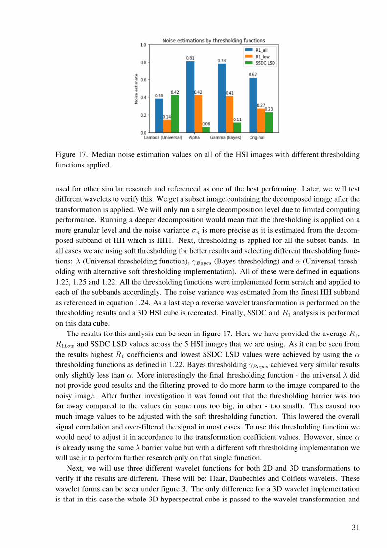
Figure 17. Median noise estimation values on all of the HSI images with different thresholdingfunctions applied.

used for other similar research and referenced as one of the best performing. Later, we will testdifferent wavelets to verify this. We get a subset image containing the decomposed image after thetransformation is applied. We will only run a single decomposition level due to limited computingperformance. Running a deeper decomposition would mean that the thresholding is applied on amore granular level and the noise variance σn is more precise as it is estimated from the decom-posed subband of HH which is HH1. Next, thresholding is applied for all the subset bands. Inall cases we are using soft thresholding for better results and selecting different thresholding func-tions: λ (Universal thresholding function), γBayes (Bayes thresholding) and α (Universal thresh-olding with alternative soft thresholding implementation). All of these were defined in equations1.23, 1.25 and 1.22. All the thresholding functions were implemented form scratch and applied toeach of the subbands accordingly. The noise variance was estimated from the finest HH subbandas referenced in equation 1.24. As a last step a reverse wavelet transformation is performed on thethresholding results and a 3D HSI cube is recreated. Finally, SSDC and R1 analysis is performedon this data cube.

The results for this analysis can be seen in figure 17. Here we have provided the average R1,R1Low and SSDC LSD values across the 5 HSI images that we are using. As it can be seen fromthe results highest R1 coefficients and lowest SSDC LSD values were achieved by using the αthresholding functions as defined in 1.22. Bayes thresholding γBayes achieved very similar resultsonly slightly less than α. More interestingly the final thresholding function - the universal λ didnot provide good results and the filtering proved to do more harm to the image compared to thenoisy image. After further investigation it was found out that the thresholding barrier was toofar away compared to the values (in some runs too big, in other - too small). This caused toomuch image values to be adjusted with the soft thresholding function. This lowered the overallsignal correlation and over-filtered the signal in most cases. To use this thresholding function wewould need to adjust it in accordance to the transformation coefficient values. However, since αis already using the same λ barrier value but with a different soft thresholding implementation wewill use ir to perform further research only on that single function.

Next, we will use three different wavelet functions for both 2D and 3D transformations toverify if the results are different. These will be: Haar, Daubechies and Coiflets wavelets. Thesewavelet forms can be seen under figure 3. The only difference for a 3D wavelet implementationis that in this case the whole 3D hyperspectral cube is passed to the wavelet transformation and

31

Figure 18. Band correlation coefficient R1 plot for two hyperspectral images across all wave-lengths before and after 2D and 3D DWT filtering was applied. On the left - hyperspectral imageHSI-5 (5) correlation coefficient R1 plot for 2D DWT filtering. On the right - hyperspectral imageHSI-5 (5) correlation coefficient R1 plot for 3D DWT filtering.

decomposition instead of each band separately. The HH subband in this case is a 3D smallertransformation cube. The schema for this can be seen under figure 4. Also, we are using onlythe α thresholding function as it performed the best out of the rest. The correlation coefficient R1

analysis results for all of the wavelet forms after filtering for HSI-5 (5) can be seen in figure 18.As it can be seen from figure 18 2D and 3D Wavelet filtering results were very similar. For the

2D DWT there were no dependencies found on the Wavelet form. Coiflets wavelet outperformedHaar and Daubechies wavelets only by 0.1%. This small change will not be taken into account andfurther research will be performed only on a single Coiflet wavelet function. However, for the 3Dwavelet filtering there were more differences between wavelets as Daubechies wavelet based 3Dfiltering outputed a non continuous spectrum. The results seemed to fluctuate arround the meanvalues. This can partially be explained when looking at the thresholding value selection. During3D wavelet thresholding the noise estimate value from equation 1.24 is estimated from data in allthe channels. It is expected that the existing noise variance is similar in all channels. However,from previous research we know that channels where λε[700; 900] are less noisy and have highercorrelation coefficients compared to λε[0; 700] channels. This affects the global noise estimatevalue and the thresholding parameter becomes less accurate. For 2D filtering in each channeliteration the noise estimate parameter is re-adjusted for that single channel. Same correlationestimation was repeated for 3D DWT with λ 10 times smaller and the R1 value variances forthat wavelet were lower. Regarding the values of R1, both 2D and 3D wavelet filtering methodsperformed similar producing similar noise value estimates. 2D DWT filtering outputed slightlyhigher values with arround 15% incrase in R1All and R1Low. Details of this increase can be seen intable 5.

SSDC analysis results can be seen in figure 19. As it can be seen from the figures, 2D DWToutperformed the 3D DWT significantly. The overall average LSD for all the images in 2D DWTwas about 2.5 times lower compared to 3D DWT. In 3D DWT the signal LM and noise LSD valuesseemed to be much closer to the original noisy images compared to 2D DWT. The only downsideis that in 2D DWT signal LM values were affected by the filtering and deviated from the originalLM values. However, this can be expected and the deviation is not too big containing much ofthe original signal shape and values. Detail results for all of noise estimate values for 2D and 3D

32

Figure 19. SSDC analysis results for HSI-5 5 before and after 2D and 3D DWT filtering wasapplied. On the left - SSDC results for 2D DWT filtering with Coiflets wavelet form. On the right- SSDC results for 3D DWT filtering with Coiflets wavelet form.

wavelet filtering can be seen in table 5. To avoid reduncancy the table only contains the changeof relative noise estimate values. The original, noisy data values can be seen in tables 1 and 3.The main reason for different results was already mentioned in R1 correlation analysis previously- different channels have different noise levels, therefore, a global σ for a global noise varianceestimate provides an inaccurate thresholding function which results in some channels not beingfiltered out at a maximum precentage. In 2D DWT this is accounted for by calculating σ for eachband.

Table 5. 2D and 3D DWT filtering results comparisons with soft thresholding applied (A - Afterfiltering, B - Before filtering).

HSI Waveletfiltering

BandcorrelationR1A/R1B

Low bandcorrelationR1A/R1B

LM signalLMA/LMB

SSDC LSDoverall valueLSDB/LSDA

1 2D 1.35 1.62 0.39 6.121 3D 1.23 1.31 0.76 2.302 2D 1.37 1.74 0.89 5.042 3D 1.23 1.26 1.18 2.103 2D 1.37 1.68 0.99 3.873 3D 1.23 1.21 1.05 2.104 2D 1.18 1.41 0.56 2.474 3D 1.23 1.21 0.95 1.215 2D 1.21 1.32 0.73 3.655 3D 1.21 1.21 0.99 1.21

2.1.7 Block Matching 3D Filtering

Next, we will implement a BM3D based filtering model which will try to filter out data based onthe BM3D algorithm. The details of this algorithm and the steps that are involved in this algorithm

33

were discussed in detail in topic 1.3.5. As mentioned in the topics, we will be using an existingBM3D library that is publicly available and acquired from http://www.cs.tut.fi/~foi/GCF-BM3D.The only difference is that this algorithm was created for denoising simple 2D images, we will beadjusting it to run for a 3D HSI data cube. Each band will be treated as a 2D image and providedas input to the algorithm. Therefore, the block matching, grouping, aggregation and all of thesteps and phases defined in the section 1.3.5 will be done only on a single band image. The finalfiltered cube will be the aggregated image of all of the bands, similar to wavelet 2D filtering. Thedownside of this, is that spectral correlations are not taken into account. Also, for each band wewill need to provide the noise variance estimate σ. This will be estimated for each band based onthe same approach we already did from wavelet based filtering. For each band we will perform a2D DWT transformation and calculate the σ from the suband HH, as defined in equations 1.24 and1.23. A IDWT is not required as we are not performing thresholding directly and only estimatingthe noise variance. Hard thresholding will be performed by the BM3D software. As in waveletfiltering SSDC and correlation coefficient R1 is going to be calculated before/after filtering todetermine the filtering results. Before discussing the results, it is worth mentioning that the wholecomputation of filtering is very performance intesive and computation time is arround 4 timeslonger compared to wavelet or median filtering. Running the filtering for a single HSI image cantake from an hour to 2 hours depending on the image size (all used HSI images contained 192bands but different pixel count). If needed to run on a big number of images which are biggerin size a high computation machine might be needed. For reference, on our tests a local personalcomputer was used with 32 GB of RAM and i7-7500U CPU 2.9 GHz with 4 cores. Extendingthe BM3D algorithm to a BM4D which would include spectral corellations would dramaticallyincrease computation time. Nevertheless, the correlation coefficent R1 and SSDC estimate resultsfor this filtering method can be seen under figures 20 and 21.

As it can be seen from the results BM3D proved to be a very good filtering method. It out-performed both 3D and 2D wavelet filtering methods in all noise estimates. The average bandcorellation coefficients R1 and R1Low were accordingly 1.44 and 3.01 times bigger compared toorignal values. SSDC results were even better - average SSDC LSD increase across all imageswas 8.77. This means the estimated noise was 8.77 times lower after the filtering compared to the

Figure 20. Band correlation coefficient R1 plot for two hyperspectral images across all wave-lengths before and after BM3D filtering was applied. On the left - hyperspectral image HSI-1 (1)correlation coefficient R1 plot for BM3D filtering. On the right - hyperspectral image HSI-5 (5)correlation coefficient R1 plot for BM3D filtering.

34

Figure 21. SSDC analysis results for two hyperspectral images before and after BM3D filteringwas applied. On the left - SSDC results for HSI-1 (1) BM3D filtering with Coiflets wavelet form.On the right - SSDC results for HSI-5 (5) BM3D filtering with Coiflets wavelet form.

original. Furthermore, LM signal values were not changed after the filtering. This means onlythe noisy LSD parts were targeted and no useful information was lost, maintining the original sig-nal shape and values. This was not demonstrated in any previous filtering methods including themedian filter. The full noise estimate values can seen in table 6.

Finally, an improved version of the BM3D algorithm was implemented by including a PCA(Principal Components Analysis) step. This in theory should have improved the BM3D resultssince the whole algorithm would be performed only on PCA output components and not on thetransformation coefficients. Full schema of the implemented algorithm can be seen in figure 9.However, in our implementation with the PCA analysis this was not proved to be the case. Thefinal output filtered HSI cube did not improve in the noise estimated values. SSDC and correlationcoefficient R1 analysis results improved only slightly compared to the original noisy cube andperformed the worst compared to the previously used filtering methods. The main reason for theseresults might be that the library responsible for BM3D filtering is not tuned to be used togetherwith PCA components as the documentation on it is limited. Another possibility is that the PCAtransformation was implemented incorrectly. However, for this analysis an existing implementa-tion of PCA transformation in Scikit learning Pyhton library was used lowering this possibility.Therefore, we will not provide any results for this analysis step as the issues were not directlydata related. However, the excellent results of the BM3D algorithm is sufficient and further, moredetail PCA analysis step seemed to not be needed.

2.1.8 Image quality analysis

Lastly, we will try to asess the filtering qualities in terms of PSNR or Peak Signal Noise Ratio. Thismethod is commonly used to compare how the filtering is effective by taking the noise-free imageand the denoised image and calculating the MSE between these two images as noted in equation1.12. The only problem we have is that we do not have a noise free image due to the nature ofthe research, so we will try to compare against the noisy image for all the filtering techniques byusing the same baseline image and try to make conclusions from that information. PSNR will becalculated for each band of the HSI cube and we will obtain a PSNR to wavelength λ relationship.Also, we will calculate the average PSNR value across all bands. This will give a single dB valuefor easier comparisons between filtering methods. The results for the image quality examination

35

Figure 22. Image quality analysis results for hyperspectral images. On the left - PSNR and λdependency for image HSI-5 (5) for different filtering techniques. On the right - Average PSNRestimation results across all the bands and all the images for different filtering techniques.

can be seen in figure 22. Here we have provided the PSNR and λ relationship for a single HSI-5(5) image and the PSNR bar chart with the mean values of PSNR across all the images for differentfiltering methods. As it can be seen from figure 22 highest PSNR values were achieved by wavelet3D filtering and BM3D filtering method. Typical PSNR values for Wavelet transformations withdifferent wavelet forms are usually between 20−30dB [21]. In our case 3D wavelet outperformed2D wavelet transformation quite significantly in this measurement (33dB and 27.6dB) which isinteresting since in other measurements (SSDC and R1) analysis 2D wavelet outperformed 3Dwavelet with lower signal information loss. The reason for this can be seen on the detail PSNRwavelength λ relationship. 3D wavelet has a significantly higher PSNR in the lower and the higherbands (λε[400; 550] and λε[900; 1000]). This is because we are using the noisy image as baselineand calculating MSE between the filtered and original as specified in equation 1.12. This meansthat the smaller the MSE between the noisy image and the filtered one - the more noise exists inthese channels. That means wavelet 3D filtering performed the worst in these wavelengths as theseare the noisiest ones (as stated by the previous analysis). The same can be said for the λε[550; 900]

inverval. Bigger PSNR means smaller differences between the filtered and the original. The keyhere is that we already know that these subbands already have a high correlation R1 and highSSDC LSD, so there is not much noise to filter in the first place, therefore, PSNR is higher in thesebands. Regarding the BM3D PSNR values - usual values as stated on 2D image denoising are

Table 6. BM3D based filtering results (A - After filtering, B - Before filtering).

HSI BandcorrelationR1A/R1B

Low bandcorrelationR1A/R1B

LM signalLMA/LMB

SSDC LSDoverall valueLSDB/LSDA

1 1.48 3.23 1 11.052 1.5 3.18 0.99 7.733 1.53 3.21 1 13.654 1.32 2.96 0.99 4.975 1.37 2.86 1 6.48

36

found between 30dB and 40dB which our implementation has achieved [31]. But as mentionedbefore on most of the similar research a clean and a filtered image is compared (which we do nothave). Therefore, looking in the absolute values should not be of most importance. Nevertheless,we have already got good insights on this PSNR analysis for our filtering methods. Lastly, we willsummarize and perform a final method comparison, and provide final recommendations.

2.1.9 Filtering method comparison

Finally, we can compare all the results for the implemented filtering methods and draw conclu-sions. The final filtering method comparisons can be seen in table 7. This table shows all theaverage noise estimate value increase of all the HSI images compared to original values. As it can

Table 7. Filtering method comparison based on average HSI noise estimate values (A - Afterfiltering, B - Before filtering).

Filteringmethod

BandcorrelationR1A/R1B

Low bandcorrelationR1A/R1B

LM signalLMA/LMB

SSDC LSDoverall valueLSDB/LSDA

PSNR,dB

Median 1.27 1.5 0.6 8.3 29Wavelet 2D 1.3 1.55 0.75 4.23 27.58Wavelet 3D 1.22 1.24 0.98 1.78 33

BM3D 1.44 3.1 1 8.76 32.12

be seen from the table the overall best performing filtering method is the BM3D. It provides thebest denoising results aswell as keeping the useful signal intact (reducing the SSDC LSD noisedeviation by more than 8 times). The PSNR value was higher only for the wavelet 3D filteringmethod. The reasons for this were already discussed previously. The only downside for using theBM3D method is that it takes a long to compute. In our research in took from 1 to 2 hours on asingle HSI data cube. Also, this method could be improved by extending the block matching algo-rithm to search for similar patches in all the bands and not only the current. This would increaseband correlation R1 dramatically but, also, dramatically increase computation time. The secondbest performing method was the 2D wavelet based transformation. This method reduced localnoise by more than 4 times and increased band correlation by more than 20%. The downside isthat the calculated PSNR value was the lowest. Although due to the missing clean image this factshould not be considered as impactful. The worst performing methods were the median filter andthe wavelet 3D. The median filter performed very good on the SSDC LSD estimation (reducingthe value by more than 8 times) but that was expected as the filter is only a simple 3x3 matrixthat computed the averages of local pixel values. This approach is very efficient at denoising buta lot of information is lost and this can be seen in the lowest LM signal value LMA/LMB. Themedian filter is not used in real world cases for denoising data with important information andin our research it was only used to create a noise evaluation methodology. Lastly, the wavelet3D performed the worst with the lowest noise estimate value increases. The LM signal value forwavelet 3D did not change much but this is due to not filtering enough noise. This can be con-cluded by looking into the PSNR value and the overall SSDC LSD value. The reasons for thiswere discussed previously but the main issue is that the thresholding parameter cannot be used for

37

all the bands as a global threshold value. The σn value must be calculated for each of the bandseparately as the noise levels are quite different in each band (as it is done in wavelet 2D filtering).

The results for the noise method evaluation were already covered in section 2.1.5. Here wewill only mention the key factors. Initially the noise evaluation was supposed to be performedfor LMLSD LSD and SSDC LSD but since LMLSD method was found as not being reliableenough it was not used to perform more complex filtering. Pixel correlation R2 method was alsonot used in further analysis mainly due not having a need for it as SSDC LSD already coveredneighboring pixel and band correlations. However, the method could be used when there is a needto analyze the provided HSI images if they are continuous and represent single substances. Forexample, if we had an image where multiple different objects were found (grain fields, houses,trees etc.) we could identify different regions of the image where the correlation coefficient R2

was similar. Also, it could be used for image slicing as usually the corners of these images have alower correlation R2 coefficients due to hyperspectral camera lensing. Finally, as a last conclusionwe would recommend using the BM3D filtering technique for HSI image denoising and SSDCLSD (optionally R1, R2 correlation methods) for evaluating noise.

38

Conclusions and Recommendations

1. In this research paper we have analyzed hyperspectral images, hyperspectral imaging tech-nologies and the noise origins in hyperspectral images. We have analyzed and implementedmultiple HSI noise evaluation methods: correlation coefficient based (R1 and R2) and linearreggression based (LMLSD and SSDC). To compare different noise evaluation methods wehave implemented a median filter as described in section 1.3.1. For the analysis we haveused 5 different noisy hyperspectral crop images captured from an airborne drone. We haveconcluded that in all noise evaluation methods the noise estimate parameter values werelower after filtering than in the original image, therefore, concluding that our designed noiseevaluation methodology can be used to represent noise levels in HSI images.

2. After analyzing the different noise evaluation methods we have concluded that the corre-lation coefficient based estimate methods and the linear reggresion based methods all givedifferent results on how effective the filtering is. This is because our knowledge of the ini-tial noise found in the images is limited. Therefore, we cannot say which of the methodsrepresent the existing noise in the most accurate way. Nevertheless, we have concluded thatthe linear reggresion based algorithm LMLSD - does not provide accurate results in estimat-ing the whole HSI data cube noise. The main reasons for the inaccurate results are due tothe images not being fully homogeneous with varying noise levels on different bands whichcaused LMLSD LSD to provide inaccurate and inconsistent results. However, the other im-plemented methods - SSDC, R1 correlation coefficient and pixel correlation R2 providedwith similar results on determinig which are the most noisy bands and two of them wereused to evaluate advanced filtering algorithms.

3. More advanced filtering algorithms were implemented and compared. The best results weregiven by the BM3D algorithm which outperformed wavelet 2D, 3D and the basic medianfilter in all noise estimate parameters. More importantly it did not change the original signalLM values and the initial signal remained intact after filtering (full results in table 7). Thiswas not demonstrated by any other method and this method is our recommendation fordenoising HSI images. Direct 2D and 3D Wavelet Transformation based filtering was, also,implemented with different threshold functions and different wavelet forms. It was foundthat there are minimum dependencies on the selected wavelet form but big dependencieson thresholding functions. The best results were achieved with the λ threshold parameterand α threshold function (equations 1.23, 1.22). 3D DWT based filtering performed worsecompared to 2D due to images not having homogeneous noise in all bands and, therefore,impacting the thresholding parameter accuracy. As expected, median filtered provided goodSSDC LSD results but it had the biggest changes in signal LM values, changing the originaluseful signal information.

4. Finally, Peak-Signal-To-Noise (PSNR) Ratio parameter (equation 1.12) was calculated toasess image quality for different filtering technologies. The results showed that the worstperforming method was the wavelet 3D. Other methods provided simillar results with BM3Dhaving the highest PSNR values in λε[550; 900] inverval and lowest in λε[400; 550] andλε[900; 1000]. This means the biggest filtering was done the lowest and highest bands, andleast filtering was done in mid-range. Therefore, concluding that the BM3D targeted thenoisiest channels for the filtering leaving the least noisy intact.

39

Future research work

As discussed throughout the research project there are multiple possibilities for a research workextension. These will be sumarized in the following list:

1. Comparing different noise evaluation methods with known noise origins. Another issue thatwas encountered in the HSI analysis was that the initial noise and what kind of noise (Gaus-sian, impulse, periodic etc.) was in the images was not known. Without that knowledgeit is too hard to clearly tell which of the noise evalution methods were the most accuratesince they showed different noise parameter levels. This can be solved by running the noiseevaluation metohds on HSI where the initial noise is known. This can be done by finding aclean HSI and adding artificial noise (Gaussian, Periodic, Impulse etc.) on it. Afterwards,denoising with the noise removal techniques and cross checking the correct PSNR with ournoise estimate parameters.

2. Finding the best performing thresholding function to use with the 2D DWT transformation.As it was found in the research there is a high dependency for denoising results on whichthresholding function is used and what is the thresholding parameter. A more detail researchcould be performed by implementing more complex thresholding functions such as heasure,minimax, rigsure thresholding functions.

3. Implementing more and different advanced noise removal techniques. In current researchwe only deeply looked at BM3D and wavelet based denoising. Even though these two arethe most popular ones there are other techniques that could be tried out.

40

References

[1] Continuous wavelet transform and scale-based analysis. http://www.mathworks.com/help/wavelet/gs/continuous-wavelet-transform-and-scale-based-analysis.html. Accessed: 2019-11-15.

[2] Rajeev Aggarwal, Jai Karan Singh, Vijay Kumar Gupta, Sanjay Rathore, Mukesh Tiwari, andAnubhuti Khare. Noise reduction of speech signal using wavelet transform with modifieduniversal threshold. International Journal of Computer Applications, 20(5):14--19, 2011.

[3] Tudor Barbu. Variational image denoising approach with diffusion porous media flow. InAbstract and Applied Analysis, volume 2013. Hindawi, 2013.

[4] Antoni Buades, Bartomeu Coll, and J-M Morel. A non-local algorithm for image denoising.In 2005 IEEE Computer Society Conference on Computer Vision and Pattern Recognition(CVPR’05), volume 2, pages 60--65. IEEE, 2005.

[5] Antoni Buades, Bartomeu Coll, and Jean Michel Morel. On image denoising methods. CMLAPreprint, 5, 2004.

[6] Antoni Buades, Bartomeu Coll, and Jean-Michel Morel. Non-local means denoising. ImageProcessing On Line, 1:208--212, 2011.

[7] Dr Philippe Cattin. Image restoration: Introduction to signal and image processing. MIAC,University of Basel. Retrieved, 11:93, 2013.

[8] Juan Cebrion and Carlos Travieso. 2-D Discrete Wavelet Transform for Hand Palm TextureBiometric Identification and Verification. 03 2012.

[9] Yakup Cengiz and Yard Doc Umut Arıöz. An application for speech denoising using discretewavelet transform. In 2016 20th National Biomedical Engineering Meeting (BIYOMUT),pages 1--4. IEEE, 2016.

[10] S Grace Chang, Bin Yu, and Martin Vetterli. Adaptive wavelet thresholding for image de-noising and compression. IEEE transactions on image processing, 9(9):1532--1546, 2000.

[11] Guangyi Chen, Tien D Bui, Kha Gia Quach, and Shen-En Qian. Denoising hyperspectral im-agery using principal component analysis and block-matching 4d filtering. Canadian Journalof Remote Sensing, 40(1):60--66, 2014.

[12] Cigdem Polat Dautov and Mehmet Sirac Özerdem. Introduction to wavelets and their appli-cations in signal denoising. Bitlis Eren University Journal of Science & Technology, 8(1),2018.

[13] Igor Djurović. Bm3d filter in salt-and-pepper noise removal. EURASIP Journal on Imageand Video Processing, 2016(1):13, 2016.

[14] David L Donoho and Jain M Johnstone. Ideal spatial adaptation by wavelet shrinkage.biometrika, 81(3):425--455, 1994.

[15] Alexandre Y Fong and Elliot Wachman. Hyperspectral imaging for the life sciences. Bio-photonics International, 15(3):38, 2008.

41

[16] Lianru Gao, Qian Du, Bing Zhang, Wei Yang, and Yuanfeng Wu. A comparative study onlinear regression-based noise estimation for hyperspectral imagery. IEEE Journal of SelectedTopics in Applied Earth Observations and Remote Sensing, 6(2):488--498, 2013.

[17] Rafael C Gonzalez and Richard E Woods. Image processing. Digital image processing, 2:1,2007.

[18] Rafael C Gonzalez, Richard E Woods, et al. Digital image processing [m]. Publishing houseof electronics industry, 141(7), 2002.

[19] Xavier Heurtebise and Sébastien Thon. Discrete tools for virtual sculpture. pages 415--422,01 2006.

[20] Timo Hyvärinen. What makes push-broom hyperspectral imaging advantageous for art ap-plications. SPECIM, Spectral Imaging Ltd, page 9, 2016.

[21] Mohideen Kother, Perumal Arumuga, Krishnan Nallaperumal, and Mohamed Sathik. Imagedenoising and enhancement using multiwavelet with hard threshold in digital mammographicimages. International Arab Journal of e-Technology, 2, 01 2011.

[22] Marc Lebrun. An analysis and implementation of the bm3d image denoising method. ImageProcessing On Line, 2:175--213, 2012.

[23] Amy Lowe, Nicola Harrison, and Andrew P. French. Hyperspectral image analysis tech-niques for the detection and classification of the early onset of plant disease and stress. PlantMethods, 13(1):80, Oct 2017.

[24] Guomin Luo, Daming Zhang, and DD Baleanu. Wavelet denoising. Advances in wavelettheory and their applications in engineering, physics and technology, page 634, 2012.

[25] Anne-Katrin Mahlein. Plant disease detection by imaging sensors – parallels and specificdemands for precision agriculture and plant phenotyping. Plant Disease, 100(2):241--251,2016. PMID: 30694129.

[26] Michel Misiti, Yves Misiti, Georges Oppenheim, Jean-Michel Poggi, et al. Wavelet toolboxuser’s guide. The Math Works Ins, 1996.

[27] Yusuf Perwej, Firoj Parwej, and Asif Perwej. Copyright protection of digital images us-ing robust watermarking based on joint dlt and dwt. International Journal of Scientific &Engineering Research, 3(6):1--9, 2012.

[28] Behnood Rasti, Paul Scheunders, Pedram Ghamisi, Giorgio Licciardi, and Jocelyn Chanus-sot. Noise reduction in hyperspectral imagery: Overview and application. Remote Sensing,10(3):482, 2018.

[29] Behnood Rasti, Johannes R Sveinsson, Magnus O Ulfarsson, and Jon Atli Benediktsson.Hyperspectral image denoising using 3d wavelets. In 2012 IEEE International Geoscienceand Remote Sensing Symposium, pages 1349--1352. IEEE, 2012.

[30] Serge Savary, Andrea Ficke, Jean-No Aubertot, and Clayton Hollier. Crop losses due todiseases and their implications for global food production losses and food security. FoodSecurity, 4(4):519--537, Dec 2012.

42

[31] Department of Signal Processing TAMPERE UNIVERSITY OF TECHNOLOGY. Imageand video denoising by sparse 3D transform-domain collaborative filtering. http://www.cs.tut.fi/~foi/GCF-BM3D/, 2019. [Online; accessed 20-12-2019].

[32] Pekka J Toivanen, Arto Kaarna, Jarno S Mielikainen, and Mikko Laukkanen. Noise reductionmethods for hyperspectral images. In Image and Signal Processing for Remote Sensing Viii,volume 4885, pages 307--314. International Society for Optics and Photonics, 2003.

[33] Yu Wang, Nicholas P. Reder, Soyoung Kang, Adam Glaser, and Jonathan Liu. Multi-plexed optical imaging of tumor-directed nanoparticles: A review of imaging systems andapproaches. Nanotheranostics, 1:369--388, 08 2017.

43