adaptive eye-camera calibration for head-worn devices...adaptive eye-camera calibration for...
TRANSCRIPT

Adaptive Eye-Camera Calibration for Head-Worn Devices
David Perra1, Rohit Kumar Gupta2, Jan-Micheal Frahm2
1Google Inc.2The University of North Carolina at Chapel Hill.
[email protected], {rkgupta,jmf}@cs.unc.edu
Abstract
We present a novel, continuous, locally optimal calibra-
tion scheme for use with head-worn devices. Current cal-
ibration schemes solve for a globally optimal model of the
eye-device transformation by performing calibration on a
per-user or once-per-use basis. However, these calibra-
tion schemes are impractical for real-world applications
because they do not account for changes in calibration dur-
ing the time of use. Our calibration scheme allows a head-
worn device to calculate a locally optimal eye-device trans-
formation on demand by computing an optimal model from
a local window of previous frames. By leveraging naturally
occurring interest regions within the user’s environment,
our system can calibrate itself without the user’s active par-
ticipation. Experimental results demonstrate that our pro-
posed calibration scheme outperforms the existing state of
the art systems while being significantly less restrictive to
the user and the environment.
1. Introduction
We are now at the verge of ubiquitously available
consumer-grade head-wearable devices, with Google Glass
serving as an early example. These devices enable new
ways of interacting with the environment but also present
challenges for meaningful interaction with the device. Cur-
rently, the most dominant mode of interaction with head-
worn devices is voice control, which allows for the trigger-
ing of preset tasks. However, this form of control is tedious
for applications such as photography (for example, taking
a controlled snapshot of a scene by zooming in on only a
particular part of the scene; see Figure 1 for an example of
a controlled photo). A natural alternative in controlling the
camera’s viewpoint is to allow the user’s gaze to guide the
photo-taking process. This becomes especially interesting
now that there are cameras available that allow full digital
zoom at the native sensor resolution by only selecting a part
of the sensor for the photo; such a camera is already found
on-board in the Nokia Lumia 1020. For these devices, it is
Full Image Plane
Camera
User’s Eye
Controlled Subimage
based on User’s Gaze
User Gaze
Wide - angle View
from Scene -
facing C amera
User’s Eye
User’s Gaze
Point of Regard
Subregion
Captured by
Scene - facing
Camera
Figure 1: A diagram of a photography scenario in which
the captured image’s focal point is controlled by the user’s
gaze.
critical to select the correct sensor region based on the user’s
gaze at the time of capture. We propose a gaze tracking
system for head-worn devices using a user-facing camera
to extract the user’s gaze. In addition, the proposed system
can generally be used to determine the direction of user’s at-
tention by estimating their 3D point of regard (PoR) in the
environment. The PoR can in turn be used for photography,
safety notifications, analyzing user’s social interaction, and
other aids to the human visual system. Our PoR estimation
technique is especially useful to a number of emerging re-
search fields, including those focused upon human behavior
and social interaction; these fields are forced to choose be-
tween overly cumbersome gaze tracking hardware (which
may affect the subjects’ behaviors or interactions) or at-
tempting gaze estimation from face pose alone, losing out
on gaze subtleties from eye-only gaze adjustments [18, 8].
Recent video-based eye tracking systems can be divided
into two groups: 1. Appearance-based methods use the eye
1
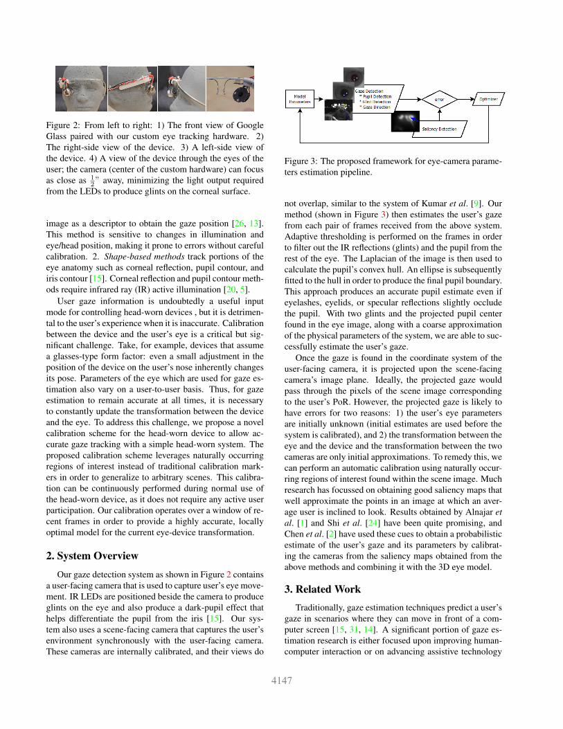
Figure 2: From left to right: 1) The front view of Google
Glass paired with our custom eye tracking hardware. 2)
The right-side view of the device. 3) A left-side view of
the device. 4) A view of the device through the eyes of the
user; the camera (center of the custom hardware) can focus
as close as 1
2” away, minimizing the light output required
from the LEDs to produce glints on the corneal surface.
image as a descriptor to obtain the gaze position [26, 13].
This method is sensitive to changes in illumination and
eye/head position, making it prone to errors without careful
calibration. 2. Shape-based methods track portions of the
eye anatomy such as corneal reflection, pupil contour, and
iris contour [15]. Corneal reflection and pupil contour meth-
ods require infrared ray (IR) active illumination [20, 5].
User gaze information is undoubtedly a useful input
mode for controlling head-worn devices , but it is detrimen-
tal to the user’s experience when it is inaccurate. Calibration
between the device and the user’s eye is a critical but sig-
nificant challenge. Take, for example, devices that assume
a glasses-type form factor: even a small adjustment in the
position of the device on the user’s nose inherently changes
its pose. Parameters of the eye which are used for gaze es-
timation also vary on a user-to-user basis. Thus, for gaze
estimation to remain accurate at all times, it is necessary
to constantly update the transformation between the device
and the eye. To address this challenge, we propose a novel
calibration scheme for the head-worn device to allow ac-
curate gaze tracking with a simple head-worn system. The
proposed calibration scheme leverages naturally occurring
regions of interest instead of traditional calibration mark-
ers in order to generalize to arbitrary scenes. This calibra-
tion can be continuously performed during normal use of
the head-worn device, as it does not require any active user
participation. Our calibration operates over a window of re-
cent frames in order to provide a highly accurate, locally
optimal model for the current eye-device transformation.
2. System Overview
Our gaze detection system as shown in Figure 2 contains
a user-facing camera that is used to capture user’s eye move-
ment. IR LEDs are positioned beside the camera to produce
glints on the eye and also produce a dark-pupil effect that
helps differentiate the pupil from the iris [15]. Our sys-
tem also uses a scene-facing camera that captures the user’s
environment synchronously with the user-facing camera.
These cameras are internally calibrated, and their views do
Figure 3: The proposed framework for eye-camera parame-
ters estimation pipeline.
not overlap, similar to the system of Kumar et al. [9]. Our
method (shown in Figure 3) then estimates the user’s gaze
from each pair of frames received from the above system.
Adaptive thresholding is performed on the frames in order
to filter out the IR reflections (glints) and the pupil from the
rest of the eye. The Laplacian of the image is then used to
calculate the pupil’s convex hull. An ellipse is subsequently
fitted to the hull in order to produce the final pupil boundary.
This approach produces an accurate pupil estimate even if
eyelashes, eyelids, or specular reflections slightly occlude
the pupil. With two glints and the projected pupil center
found in the eye image, along with a coarse approximation
of the physical parameters of the system, we are able to suc-
cessfully estimate the user’s gaze.
Once the gaze is found in the coordinate system of the
user-facing camera, it is projected upon the scene-facing
camera’s image plane. Ideally, the projected gaze would
pass through the pixels of the scene image corresponding
to the user’s PoR. However, the projected gaze is likely to
have errors for two reasons: 1) the user’s eye parameters
are initially unknown (initial estimates are used before the
system is calibrated), and 2) the transformation between the
eye and the device and the transformation between the two
cameras are only initial approximations. To remedy this, we
can perform an automatic calibration using naturally occur-
ring regions of interest found within the scene image. Much
research has focussed on obtaining good saliency maps that
well approximate the points in an image at which an aver-
age user is inclined to look. Results obtained by Alnajar et
al. [1] and Shi et al. [24] have been quite promising, and
Chen et al. [2] have used these cues to obtain a probabilistic
estimate of the user’s gaze and its parameters by calibrat-
ing the cameras from the saliency maps obtained from the
above methods and combining it with the 3D eye model.
3. Related Work
Traditionally, gaze estimation techniques predict a user’s
gaze in scenarios where they can move in front of a com-
puter screen [15, 31, 14]. A significant portion of gaze es-
timation research is either focused upon improving human-
computer interaction or on advancing assistive technology
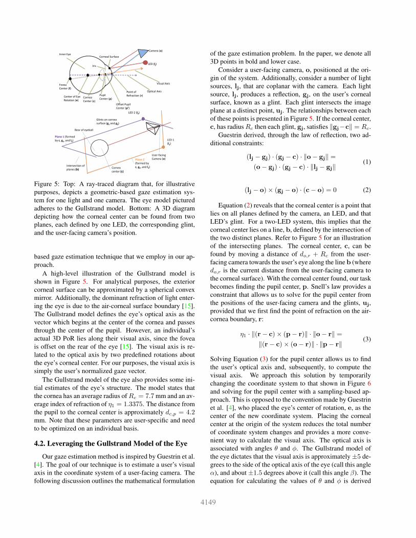
Figure 4: Simulated eye (left) and a Point of Regard square
box object (right) in the scene which the simulated eye fol-
lows.
for the impaired [29, 10, 3, 11]. As wearable devices have
become more widely used, gaze estimation has also been
explored for systems with see-through displays [27, 17];
however, all these gaze tracking systems require a careful
pre-calibration and rely upon a stable calibration throughout
their use. For head-worn devices, the calibration typically
changes during use as well as when the device is taken off or
put on. It is not practical to have the user actively perform a
calibration procedure every time the device’s pose changes.
In contrast to the existing state-of-the-art approaches, our
technique performs a continuous calibration of the device
in a simple way by utilizing the user’s natural gaze in pre-
vious frames and observing salient areas of interest within
the scene.
Hansen et al. [5] compared several different approaches,
most of which estimate the user’s point of regard (PoR).
The PoR techniques presented in their paper map a user’s
gaze onto a computer screen that is in a fixed relative pose
with respect to the user [15]. On the contrary, our approach
finds the PoR by relating the user’s gaze to automatically
detected salient regions of interest within the scene, break-
ing the requirement for a known scene geometry and known
user-to-camera settings.
Typically, the initial calibration required for accurate
gaze tracking involves the user’s active cooperation by look-
ing at a number of predefined points [30, 16]. Sugano et al.
[25] achieved an error-corrected two-eye gaze estimate by
showing natural images/videos to the user and leveraging
saliency maps to determine what object was being looked
at by the user. Their results show that combining saliency
metrics, including face detection, allows for better modeling
of the human visual system. Our method takes this concept
further by using salient areas found within the real world as
an indication of the user’s gaze direction during our calibra-
tion process.
Tsukada et al. [28] presented a system that determines
the user’s PoR by extracting the gaze from a single eye and
leveraging an appearance code book for the gaze mapping.
This appearance code book is very sensitive to the calibra-
tion, which is performed in a constrained environment and
assumed to be constant throughout use. This assumption
is not always valid due to configuration and environmental
changes. In contrast, our method does not require a global
calibration and is continuously recalibrating the configura-
tion of the user with respect to the head-worn device .
Nakazawa et al. [16] demonstrated a gaze estimation sys-
tem which projects a coded light pattern upon the scene
using a multispectral LED array. Martinez et al. [13] in-
ferred the gaze by relying upon appearance-based gaze es-
timation; they handled relative pose changes between the
device and the user by estimating the eye-device transfor-
mation using a motion capture system in their testing envi-
ronment. These techniques produce state-of-the-art results
but rely upon specialized hardware that is not found in gen-
eral environments.
Pirri et al. [21, 22] proposed a procedure for calibrating a
scene-facing camera’s pose with respect to the user’s gaze.
While effective, the technique’s dependence upon artificial
markers in the scene prevents generalization. Santner et al.
[23] built upon the research done by Pirri et al. by combin-
ing 3D saliency with a dense reconstruction of the user’s
environment for the purposes of user localization. Aside
from requiring the gaze from both eyes, their method as-
sumes a static environment premapped by a Kinect sensor,
and it thus is unable to handle dynamic scenes. In contrast,
our proposed approach neither relies on static scenes nor
requires any knowledge of scene depth.
In recent years, many researchers have devised models to
generate better-quality saliency maps. Among these, Graph
Based Visual Saliency (GBVS) [6], Adaptive Whitening
Saliency (AWS) [12], and Image Signature (ImgSig) [7]
usually exhibit the best performance. Recently, Shi et al.
[24] proposed a Reverse Hierarchy Model (RHM) for pre-
dicting eye fixations. This method also provides a compu-
tational model for saliency detection in images.
Chen et al. [2] estimated the probability distributions of
the eye parameters and eye gaze by combining an image
saliency map with the 3D eye model. They used an incre-
mental learning framework and avoided any personal cal-
ibration for the user. Our approach also uses a similar but
different framework. Alnajar et al. [1] also developed an ap-
proach to auto-calibrate gaze estimators in an uncalibrated
setup. Although this method used information from both
eyes, additional stimulus signals were exploited to estimate
gaze patterns obtained from specific users.
4. Background
Next, we introduce the basic concepts used in our ap-
proach for automatic continuous calibration of head-worn
devices.
4.1. Gullstrand Model of the Eye
The Gullstrand model is a simplified representation of
the human eye. This model is used in the geometric model-
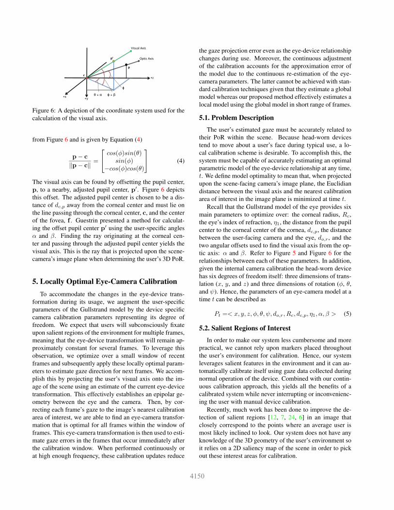
Camera (o)
LED (lj)
Pupil
Center (p) Cornea
Center (c)
Center of Eye
Rotation (e)
Fovea
Center (f)
Point of
Refraction (r)
Corneal Surface
Iris
Inner Eye
Offset Pupil
Center (p’)
Optical Axis
Visual Axis
Plane 1 (formed
by c, g1, and l1)
Plane 2
(formed by
c, g2, and l2)
User-facing
Camera (o)
LED 1
(l1)
LED 2 (l2)
Glints on cornea
surface (g1 and g2)
Cornea
center (c)
Intersection of
planes (b)
Rear of eyeball
Figure 5: Top: A ray-traced diagram that, for illustrative
purposes, depicts a geometric-based gaze estimation sys-
tem for one light and one camera. The eye model pictured
adheres to the Gullstrand model. Bottom: A 3D diagram
depicting how the corneal center can be found from two
planes, each defined by one LED, the corresponding glint,
and the user-facing camera’s position.
based gaze estimation technique that we employ in our ap-
proach.
A high-level illustration of the Gullstrand model is
shown in Figure 5. For analytical purposes, the exterior
corneal surface can be approximated by a spherical convex
mirror. Additionally, the dominant refraction of light enter-
ing the eye is due to the air-corneal surface boundary [15].
The Gullstrand model defines the eye’s optical axis as the
vector which begins at the center of the cornea and passes
through the center of the pupil. However, an individual’s
actual 3D PoR lies along their visual axis, since the fovea
is offset on the rear of the eye [15]. The visual axis is re-
lated to the optical axis by two predefined rotations about
the eye’s corneal center. For our purposes, the visual axis is
simply the user’s normalized gaze vector.
The Gullstrand model of the eye also provides some ini-
tial estimates of the eye’s structure. The model states that
the cornea has an average radius ofRc = 7.7 mm and an av-
erage index of refraction of η1 = 1.3375. The distance from
the pupil to the corneal center is approximately dc,p = 4.2mm. Note that these parameters are user-specific and need
to be optimized on an individual basis.
4.2. Leveraging the Gullstrand Model of the Eye
Our gaze estimation method is inspired by Guestrin et al.
[4]. The goal of our technique is to estimate a user’s visual
axis in the coordinate system of a user-facing camera. The
following discussion outlines the mathematical formulation
of the gaze estimation problem. In the paper, we denote all
3D points in bold and lower case.
Consider a user-facing camera, o, positioned at the ori-
gin of the system. Additionally, consider a number of light
sources, lj, that are coplanar with the camera. Each light
source, lj, produces a reflection, gj, on the user’s corneal
surface, known as a glint. Each glint intersects the image
plane at a distinct point, uj. The relationships between each
of these points is presented in Figure 5. If the corneal center,
c, has radiusRc then each glint, gj, satisfies ‖gj−c‖ = Rc.
Guestrin derived, through the law of reflection, two ad-
ditional constraints:
(lj − gj) · (gj − c) · ‖o− gj‖ =
(o− gj) · (gj − c) · ‖lj − gj‖(1)
(lj − o)× (gj − o) · (c− o) = 0 (2)
Equation (2) reveals that the corneal center is a point that
lies on all planes defined by the camera, an LED, and that
LED’s glint. For a two-LED system, this implies that the
corneal center lies on a line, b, defined by the intersection of
the two distinct planes. Refer to Figure 5 for an illustration
of the intersecting planes. The corneal center, c, can be
found by moving a distance of do,r + Rc from the user-
facing camera towards the user’s eye along the line b (where
do,r is the current distance from the user-facing camera to
the corneal surface). With the corneal center found, our task
becomes finding the pupil center, p. Snell’s law provides a
constraint that allows us to solve for the pupil center from
the positions of the user-facing camera and the glints, uj,
provided that we first find the point of refraction on the air-
cornea boundary, r:
η1 · ‖(r− c)× (p− r)‖ · ‖o− r‖ =
‖(r− c)× (o− r)‖ · ‖p− r‖(3)
Solving Equation (3) for the pupil center allows us to find
the user’s optical axis and, subsequently, to compute the
visual axis. We approach this solution by temporarily
changing the coordinate system to that shown in Figure 6
and solving for the pupil center with a sampling-based ap-
proach. This is opposed to the convention made by Guestrin
et al. [4], who placed the eye’s center of rotation, e, as the
center of the new coordinate system. Placing the corneal
center at the origin of the system reduces the total number
of coordinate system changes and provides a more conve-
nient way to calculate the visual axis. The optical axis is
associated with angles θ and φ. The Gullstrand model of
the eye dictates that the visual axis is approximately ±5 de-
grees to the side of the optical axis of the eye (call this angle
α), and about ±1.5 degrees above it (call this angle β). The
equation for calculating the values of θ and φ is derived
+y
+z
+x
Visual Axis
Optic Axis p’
p
ϕ
ϕ + β
θ + α
c
Figure 6: A depiction of the coordinate system used for the
calculation of the visual axis.
from Figure 6 and is given by Equation (4)
p− c
‖p− c‖=
cos(φ)sin(θ)sin(φ)
−cos(φ)cos(θ)
(4)
The visual axis can be found by offsetting the pupil center,
p, to a nearby, adjusted pupil center, p′. Figure 6 depicts
this offset. The adjusted pupil center is chosen to be a dis-
tance of dc,p away from the corneal center and must lie on
the line passing through the corneal center, c, and the center
of the fovea, f . Guestrin presented a method for calculat-
ing the offset pupil center p′ using the user-specific angles
α and β. Finding the ray originating at the corneal cen-
ter and passing through the adjusted pupil center yields the
visual axis. This is the ray that is projected upon the scene-
camera’s image plane when determining the user’s 3D PoR.
5. Locally Optimal Eye-Camera Calibration
To accommodate the changes in the eye-device trans-
formation during its usage, we augment the user-specific
parameters of the Gullstrand model by the device specific
camera calibration parameters representing its degree of
freedom. We expect that users will subconsciously fixate
upon salient regions of the environment for multiple frames,
meaning that the eye-device transformation will remain ap-
proximately constant for several frames. To leverage this
observation, we optimize over a small window of recent
frames and subsequently apply these locally optimal param-
eters to estimate gaze direction for next frames. We accom-
plish this by projecting the user’s visual axis onto the im-
age of the scene using an estimate of the current eye-device
transformation. This effectively establishes an epipolar ge-
ometry between the eye and the camera. Then, by cor-
recting each frame’s gaze to the image’s nearest calibration
area of interest, we are able to find an eye-camera transfor-
mation that is optimal for all frames within the window of
frames. This eye-camera transformation is then used to esti-
mate gaze errors in the frames that occur immediately after
the calibration window. When performed continuously or
at high enough frequency, these calibration updates reduce
the gaze projection error even as the eye-device relationship
changes during use. Moreover, the continuous adjustment
of the calibration accounts for the approximation error of
the model due to the continuous re-estimation of the eye-
camera parameters. The latter cannot be achieved with stan-
dard calibration techniques given that they estimate a global
model whereas our proposed method effectively estimates a
local model using the global model in short range of frames.
5.1. Problem Description
The user’s estimated gaze must be accurately related to
their PoR within the scene. Because head-worn devices
tend to move about a user’s face during typical use, a lo-
cal calibration scheme is desirable. To accomplish this, the
system must be capable of accurately estimating an optimal
parametric model of the eye-device relationship at any time,
t. We define model optimality to mean that, when projected
upon the scene-facing camera’s image plane, the Euclidian
distance between the visual axis and the nearest calibration
area of interest in the image plane is minimized at time t.
Recall that the Gullstrand model of the eye provides six
main parameters to optimize over: the corneal radius, Rc,
the eye’s index of refraction, η1, the distance from the pupil
center to the corneal center of the cornea, dc,p, the distance
between the user-facing camera and the eye, do,r, and the
two angular offsets used to find the visual axis from the op-
tic axis: α and β. Refer to Figure 5 and Figure 6 for the
relationships between each of these parameters. In addition,
given the internal camera calibration the head-worn device
has six degrees of freedom itself: three dimensions of trans-
lation (x, y, and z) and three dimensions of rotation (φ, θ,
and ψ). Hence, the parameters of an eye-camera model at a
time t can be described as
Pt =< x, y, z, φ, θ, ψ, do,r, Rc, dc,p, η1, α, β > (5)
5.2. Salient Regions of Interest
In order to make our system less cumbersome and more
practical, we cannot rely upon markers placed throughout
the user’s environment for calibration. Hence, our system
leverages salient features in the environment and it can au-
tomatically calibrate itself using gaze data collected during
normal operation of the device. Combined with our contin-
uous calibration approach, this yields all the benefits of a
calibrated system while never interrupting or inconvenienc-
ing the user with manual device calibration.
Recently, much work has been done to improve the de-
tection of salient regions [12, 7, 24, 6] in an image that
closely correspond to the points where an average user is
most likely inclined to look. Our system does not have any
knowledge of the 3D geometry of the user’s environment so
it relies on a 2D saliency map of the scene in order to pick
out these interest areas for calibration.
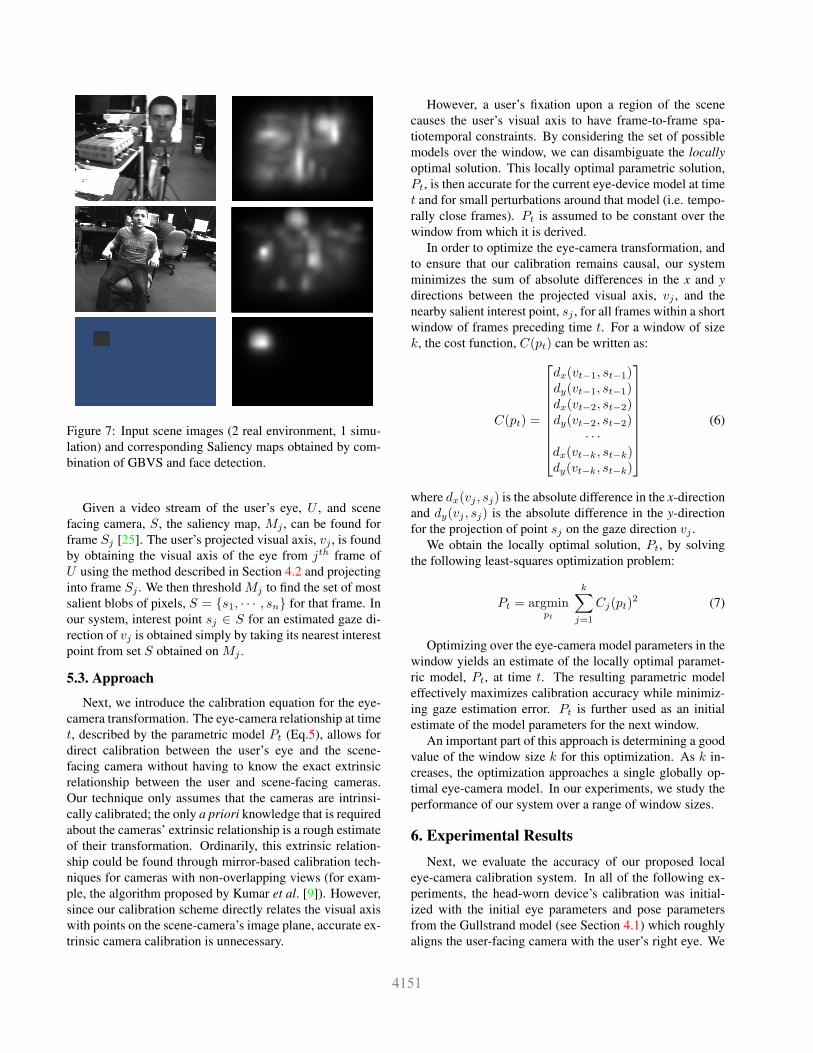
Figure 7: Input scene images (2 real environment, 1 simu-
lation) and corresponding Saliency maps obtained by com-
bination of GBVS and face detection.
Given a video stream of the user’s eye, U , and scene
facing camera, S, the saliency map, Mj , can be found for
frame Sj [25]. The user’s projected visual axis, vj , is found
by obtaining the visual axis of the eye from jth frame of
U using the method described in Section 4.2 and projecting
into frame Sj . We then threshold Mj to find the set of most
salient blobs of pixels, S = {s1, · · · , sn} for that frame. In
our system, interest point sj ∈ S for an estimated gaze di-
rection of vj is obtained simply by taking its nearest interest
point from set S obtained on Mj .
5.3. Approach
Next, we introduce the calibration equation for the eye-
camera transformation. The eye-camera relationship at time
t, described by the parametric model Pt (Eq.5), allows for
direct calibration between the user’s eye and the scene-
facing camera without having to know the exact extrinsic
relationship between the user and scene-facing cameras.
Our technique only assumes that the cameras are intrinsi-
cally calibrated; the only a priori knowledge that is required
about the cameras’ extrinsic relationship is a rough estimate
of their transformation. Ordinarily, this extrinsic relation-
ship could be found through mirror-based calibration tech-
niques for cameras with non-overlapping views (for exam-
ple, the algorithm proposed by Kumar et al. [9]). However,
since our calibration scheme directly relates the visual axis
with points on the scene-camera’s image plane, accurate ex-
trinsic camera calibration is unnecessary.
However, a user’s fixation upon a region of the scene
causes the user’s visual axis to have frame-to-frame spa-
tiotemporal constraints. By considering the set of possible
models over the window, we can disambiguate the locally
optimal solution. This locally optimal parametric solution,
Pt, is then accurate for the current eye-device model at time
t and for small perturbations around that model (i.e. tempo-
rally close frames). Pt is assumed to be constant over the
window from which it is derived.
In order to optimize the eye-camera transformation, and
to ensure that our calibration remains causal, our system
minimizes the sum of absolute differences in the x and y
directions between the projected visual axis, vj , and the
nearby salient interest point, sj , for all frames within a short
window of frames preceding time t. For a window of size
k, the cost function, C(pt) can be written as:
C(pt) =
dx(vt−1, st−1)dy(vt−1, st−1)dx(vt−2, st−2)dy(vt−2, st−2)
· · ·dx(vt−k, st−k)dy(vt−k, st−k)
(6)
where dx(vj , sj) is the absolute difference in the x-direction
and dy(vj , sj) is the absolute difference in the y-direction
for the projection of point sj on the gaze direction vj .
We obtain the locally optimal solution, Pt, by solving
the following least-squares optimization problem:
Pt = argminpt
k∑
j=1
Cj(pt)2 (7)
Optimizing over the eye-camera model parameters in the
window yields an estimate of the locally optimal paramet-
ric model, Pt, at time t. The resulting parametric model
effectively maximizes calibration accuracy while minimiz-
ing gaze estimation error. Pt is further used as an initial
estimate of the model parameters for the next window.
An important part of this approach is determining a good
value of the window size k for this optimization. As k in-
creases, the optimization approaches a single globally op-
timal eye-camera model. In our experiments, we study the
performance of our system over a range of window sizes.
6. Experimental Results
Next, we evaluate the accuracy of our proposed local
eye-camera calibration system. In all of the following ex-
periments, the head-worn device’s calibration was initial-
ized with the initial eye parameters and pose parameters
from the Gullstrand model (see Section 4.1) which roughly
aligns the user-facing camera with the user’s right eye. We

use this generic setup to show that our system can adapt to
any feasible head-device relationship.
Datasets. The performance of the proposed adaptive
eye-camera calibration framework was evaluated on 10
datasets (5 human subjects and 5 simulations). Each dataset
consists of 150-200 frames obtained from the user- and
scene-facing camera. The scene-facing camera observed a
point of regard approximately 1.1 - 1.5 meters away from
the participant. To limit the influence of confounds in the
gaze error calculation, the users were instructed to look at
the PoR and move their head in a circular fashion. For the
human subject trials, the PoR was the face of another indi-
vidual, seated at the same head level as the user. We used the
specific class of faces for the salient region detection, but
this setup could easily be generalized using saliency maps
[12, 7, 24], which would also impose similar constraints
for the eye-camera transformation. All experimental setups
have a known distance between the user and the calibration
point, which is unknown to the system and is used only for
determining our estimated gaze error. For all experiments
the head-worn device was loosely attached to user’s head to
allow natural movement during use. For quantitative evalu-
ation, we created a simulation of the whole system (see Fig-
ure 4), which generates image frames for an eye that follows
an object moving along a specified path in the 3D world.
The simulated data also contains a small, smooth perturba-
tions of the camera pose, modeling real-world changes in
the eye-camera relationship. This approach helps remove
the bias when the user is looking at a specified PoR, also it
provides a good error measurement. This model serves as
a ground truth to check the accuracy of the system, as we
have the labeled data for the gaze direction. This allows us
to obtain accurate gaze estimation errors for our system as
the ground truth is known.
Parameters. Our general eye-camera model has 12 un-
known parameters at any time t (see Section 5.1). However,
in our experiments, we fixed the refractive index η1 to a
value of 1.3375 and the cornea-to-pupil distance dc,p to 4.5
mm. As a result, we have 10 unknowns in our system that
are estimated from a window of k previous frames using the
approach specified in previous section.
After finding the locally optimal model for time t over
the window of frames at t− 1 to t− k, we analyze their ac-
curacies; each window serves as an independent calibration
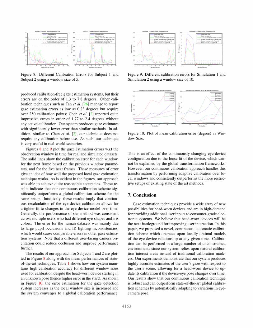
set. Results for each experiment are presented as a graph
(see Figure 8 and Figure 9) with three criteria plotted: 1)
in blue, the re-projection error from applying the locally
optimal model to the window that produced it (calibration
error), 2) in red, the error produced at time t when apply-
ing the locally optimal model (next-frame error), and 3) in
green, the mean error produced when the locally optimal
model is applied to the next five frames. We have also stud-
ied the behavior of window size k over the accuracy of the
system (Tables 1 and 2).
Table 1: Observed mean and standard deviation error (de-
grees) over all windows for a fixed window size k (simu-
lated dataset)
k 5 10 15 20 25 30
Sim 1 3.436 4.522 3.620 5.400 9.501 10.019
Sim 2 1.075 5.884 3.975 10.185 7.102 3.331
Sim 3 2.470 0.051 0.168 0.287 0.324 0.509
Sim 4 0.208 0.836 0.804 3.004 3.444 3.067
Sim 5 0.278 0.935 0.837 1.777 1.790 7.534
Mean 1.4935 2.445 1.880 4.130 4.432 4.890
Std 1.417 2.585 1.774 3.868 3.796 3.813
Table 2: Observed mean and standard deviation error (de-
grees) over all windows for a fixed window size k (human
dataset)
k 5 10 15 20 25 30
Subj 1 0.129 0.143 0.465 0.380 0.688 1.00
Subj 2 0.118 0.145 0.257 0.267 0.316 0.395
Subj 3 0.274 0.470 1.040 0.917 1.390 1.280
Subj 4 0.097 0.041 0.027 0.028 0.038 -
Subj 5 0.221 0.218 0.241 0.380 0.511 0.592
Mean 0.168 0.203 0.407 0.394 0.589 0.653
Std 0.076 0.162 0.388 0.326 0.509 0.501
We compare our method to a variety of state-of-the-art
techniques [19, 4, 1, 26, 2], though all of these require more
restrictive setups than our approach and are not able to op-
erate in loosely constrained scenarios. However, they still
provide a good reference for the proposed approach. Given
the dearth of less constrained methods, we compared the re-
ported mean calibration errors of these approaches with our
own results.
In general, a window size of 5 frames gave the best
performance for our method, with a mean accuracy of
1.493 ± 1.417 for the simulated dataset and 0.168 ± 0.076for the human subject dataset. As shown in Figure 10, ac-
curacy tends to decrease as window size increases, possi-
bly due to change in the eye-camera model parameters over
longer windows of observation. Our system achieved a per-
formance of 4-5 fps with an unoptimized matlab implemen-
tation1.
For comparison, we note that Pfeuffer et al. [19] achieve
gaze estimation errors as low as 0.55 degrees by estimating
the visual axis with 4 glints and having the user initially par-
ticipate in active calibration procedure. Guestrin et al. [4]
achieve an average gaze error of 0.9 degrees with one cali-
bration point. Recent works such as Alnajar et al. [1] have
1Code is available at http://cs.unc.edu/˜jmf/
publications/gaze_release.7z.
0 5 10 15 20 25 30 35 40 450
0.1
0.2
0.3
0.4
0.5
0.6
0.7SUBJECT 1: Locally Optimal Calibration Error
Calibration Set Number
Err
or
(de
gre
es)
Calibration error
Next−frame error
Average error for 5 additional frames
Lowest mean error for Pfeuffer et al.
Lowest mean error for Tan et al.
Mean error for our approach
0 5 10 15 20 25 30 35 40 45 500
0.1
0.2
0.3
0.4
0.5
0.6
0.7SUBJECT 2: Locally Optimal Calibration Error
Calibration Set Number
Err
or
(de
gre
es)
Calibration error
Next−frame error
Average error for 5 additional frames
Lowest mean error for Pfeuffer et al.
Lowest mean error for Tan et al.
Mean error for our approach
Figure 8: Different Calibration Errors for Subject 1 and
Subject 2 using a window size of 5.
produced calibration-free gaze estimation systems, but their
errors are on the order of 1.3 to 7.8 degrees. Other cali-
bration techniques such as Tan et al. [26] manage to report
gaze estimation errors as low as 0.23 degrees but require
over 250 calibration points; Chen et al. [2] reported quite
impressive errors in order of 1.77 to 2.4 degrees without
any active-calibration. Our system produces gaze estimates
with significantly lower error than similar methods. In ad-
dition, similar to Chen et al. [2], our technique does not
require any calibration before use. As such, our technique
is very useful in real-world scenarios.
Figures 8 and 9 plot the gaze estimation errors w.r.t the
observation window in time for real and simulated datasets.
The solid lines show the calibration error for each window,
for the next frame based on the previous window parame-
ters, and for the five next frames. These measures of error
give an idea of how well the proposed local gaze estimation
technique works. As is evident in the figures, our approach
was able to achieve quite reasonable accuracies. These re-
sults indicate that our continuous calibration scheme sig-
nificantly outperforms a global calibration scheme for the
same setup. Intuitively, these results imply that continu-
ous recalculation of the eye-device calibration allows for
a tighter fit to changes in the eye-device model over time.
Generally, the performance of our method was consistent
across multiple users who had different eye shapes and iris
colors. The error for the human datasets was mainly due
to large pupil occlusions and IR lighting inconsistencies,
which would cause comparable errors in other gaze estima-
tion systems. Note that a different user-facing camera ori-
entation could reduce occlusion and improve performance
further.
The results of our approach for Subjects 1 and 2 are plot-
ted in Figure 8 along with the mean performances of state-
of-the-art techniques. Table 1 shows how our system main-
tains high calibration accuracy for different window sizes
used for calibration despite the head-worn device starting in
an unknown pose (hence higher error in the start). As shown
in Figure 10, the error estimation for the gaze detection
system increases as the local window size is increased and
the system converges to a global calibration performance.
0 2 4 6 8 10 12 14 16 18 200
0.2
0.4
0.6
0.8
1
1.2
1.4Simulation 1: Locally Optimal Calibration Error
Window Number
Err
or
(de
gre
es)
Calibration error
Next−frame error
Average error for 5 additional frames
Lowest mean error for Pfeuffer et al.
Lowest mean error for Tan et al.
Mean error for our approach
0 5 10 150
1
2
3
4
5
6
7
8
9
10Simulation 2: Locally Optimal Calibration Error
Window Number
Err
or
(de
gre
es)
Calibration error
Next−frame error
Average error for 5 additional frames
Lowest mean error for Pfeuffer et al.
Lowest mean error for Tan et al.
Mean error for our approach
Figure 9: Different calibration errors for Simulation 1 and
Simulation 2 using a window size of 10.
5 10 15 20 25 300
0.2
0.4
0.6
0.8
1
1.2
1.4Calibration Error (degrees) versus WindowSize (Simulation)
WindowSize
Err
or
(De
gre
es)
Subject1
Subject2
Subject3
Subject4
Subject5
5 10 15 20 25 300
2
4
6
8
10
12Calibration Error (degrees) versus WindowSize (Simulation)
WindowSize
Err
or
(De
gre
es)
Simulation1
Simulation2
Simulation3
Simulation4
Simulation5
Figure 10: Plot of mean calibration error (degree) vs Win-
dow Size.
This is an effect of the continuously changing eye-device
configuration due to the loose fit of the device, which can-
not be explained by the global transformation frameworks.
However, our continuous calibration approach handles this
transformation by performing adaptive calibration over lo-
cal windows and consistently outperforms the more restric-
tive setups of existing state of the art methods.
7. Conclusion
Gaze estimation techniques provide a wide array of new
possibilities for head-worn devices and are in high-demand
for providing additional user inputs to consumer-grade elec-
tronic systems. We believe that head-worn devices will be
the next battleground for improving user interaction. In this
paper, we proposed a novel, continuous, automatic calibra-
tion scheme which operates upon locally optimal models
of the eye-device relationship at any given time. Calibra-
tion can be performed in a large number of unconstrained
environments since our system relies upon natural calibra-
tion interest areas instead of traditional calibration mark-
ers. Our experiments demonstrate that our system produces
highly accurate estimates of the user’s gaze with respect to
the user’s scene, allowing for a head-worn device to up-
date its calibration if the device-eye pose changes over time.
Our results show that our continuous calibration technique
is robust and can outperform state-of-the-art global calibra-
tion schemes by automatically adapting to variations in eye-
camera pose.
8. Acknowledgment
This material is based upon work supported by the Na-
tional Science Foundation under Grant No CNS-1405847,
NSF IIS 1423059, and US Army Research, Development
and Engineering Command Grant No W911NF-14-1-0438.
We would also like to thank True Price and Enrique Dunn
for their insights and discussions.
References
[1] F. Alnajar, T. Gevers, R. Valenti, and S. Ghebreab.
Calibration-free gaze estimation using human gaze patterns.
In 15th IEEE International Conference on Computer Vision,
2013. 2, 3, 7
[2] J. Chen and Q. Ji. Probabilistic gaze estimation without ac-
tive personal calibration. In Computer Vision and Pattern
Recognition (CVPR), 2011 IEEE Conference on, pages 609–
616, June 2011. 2, 3, 7, 8
[3] F. Corno, L. Farinetti, and I. Signorile. A cost-effective so-
lution for eye-gaze assistive technology. Multimedia and
Expo, 2002. ICME ’02. Proceedings. 2002 IEEE Interna-
tional Conference on, 2:433–436 vol.2, 2002. 3
[4] E. Guestrin and E. Eizenman. General theory of remote
gaze estimation using the pupil center and corneal reflec-
tions. Biomedical Engineering, IEEE Transactions on,
53(6):1124–1133, June 2006. 4, 7
[5] D. Hansen and Q. Ji. In the eye of the beholder: A survey
of models for eyes and gaze. Pattern Analysis and Machine
Intelligence, IEEE Transactions on, 32(3):478–500, March
2010. 2, 3
[6] J. Harel, C. Koch, and P. Perona. Graph-based visual
saliency. In ADVANCES IN NEURAL INFORMATION PRO-
CESSING SYSTEMS 19, pages 545–552. MIT Press, 2007. 3,
5
[7] X. Hou, J. Harel, and C. Koch. Image signature: Highlight-
ing sparse salient regions. IEEE Transactions on Pattern
Analysis and Machine Intelligence, 34(1):194–201, 2012. 3,
5, 7
[8] E. Jain, Y. Sheikh, and J. Hodgins. Inferring artistic intention
in comic art through viewer gaze. In ACM Symposium on
Applied Perception (SAP). 1
[9] R. Kumar, A. Ilie, J.-M. Frahm, and M. Pollefeys. Sim-
ple calibration of non-overlapping cameras with a mirror.
In Computer Vision and Pattern Recognition, 2008. CVPR
2008. IEEE Conference on, pages 1–7, June 2008. 2, 6
[10] U. Lahiri, Z. Warren, and N. Sarkar. Design of a gaze-
sensitive virtual social interactive system for children with
autism. Neural Systems and Rehabilitation Engineering,
IEEE Transactions on, 19(4):443–452, Aug 2011. 3
[11] U. Lahiri, Z. Warren, and N. Sarkar. Dynamic gaze mea-
surement with adaptive response technology in virtual reality
based social communication for autism. Virtual Rehabilita-
tion (ICVR), 2011 International Conference on, pages 1–8,
June 2011. 3
[12] V. Leborn Alvarez, A. Garca-Daz, X. Fdez-Vidal, and
X. Pardo. Dynamic saliency from adaptative whitening. In
Natural and Artificial Computation in Engineering and Med-
ical Applications, volume 7931 of Lecture Notes in Com-
puter Science, pages 345–354. Springer Berlin Heidelberg,
2013. 3, 5, 7
[13] F. Martinez, A. Carbone, and E. Pissaloux. Combining first-
person and third-person gaze for attention recognition. In
Automatic Face and Gesture Recognition (FG), 2013 10th
IEEE International Conference and Workshops on, pages 1–
6, April 2013. 2, 3
[14] A. Meyer, M. Bohme, T. Martinetz, and E. Barth. A single-
camera remote eye tracker. In Proceedings of the 2006 In-
ternational Tutorial and Research Conference on Percep-
tion and Interactive Technologies, PIT’06, pages 208–211,
Berlin, Heidelberg, 2006. Springer-Verlag. 2
[15] C. Morimoto, A. Amir, and M. Flickner. Detecting eye po-
sition and gaze from a single camera and 2 light sources. In
Pattern Recognition, 2002. Proceedings. 16th International
Conference on, volume 4, pages 314–317 vol.4, 2002. 2, 3,
4
[16] A. Nakazawa and C. Nitschke. Point of gaze estimation
through corneal surface reflection in an active illumination
environment. In A. Fitzgibbon, S. Lazebnik, P. Perona,
Y. Sato, and C. Schmid, editors, Computer Vision ECCV
2012, Lecture Notes in Computer Science, pages 159–172.
Springer Berlin Heidelberg, 2012. 3
[17] H.-M. Park, S.-H. Lee, and J.-S. Choi. Wearable augmented
reality system using gaze interaction. In Mixed and Aug-
mented Reality, 2008. ISMAR 2008. 7th IEEE/ACM Interna-
tional Symposium on, pages 175–176, Sept 2008. 3
[18] H. S. Park, E. Jain, and Y. Sheikh. 3d social saliency from
head-mounted cameras. In NIPS, pages 431–439, 2012. 1
[19] K. Pfeuffer, M. Vidal, J. Turner, A. Bulling, and
H. Gellersen. Pursuit calibration: Making gaze calibration
less tedious and more flexible. In Proceedings of the 26th
Annual ACM Symposium on User Interface Software and
Technology, UIST ’13, pages 261–270, New York, NY, USA,
2013. ACM. 7
[20] B. Pires, M. Devyver, A. Tsukada, and T. Kanade. Unwrap-
ping the eye for visible-spectrum gaze tracking on wearable
devices. In Applications of Computer Vision (WACV), 2013
IEEE Workshop on, pages 369–376, Jan 2013. 2
[21] F. Pirri, M. Pizzoli, D. Rigato, and R. Shabani. 3d saliency
maps. In Computer Vision and Pattern Recognition Work-
shops (CVPRW), 2011 IEEE Computer Society Conference
on, pages 9–14, June 2011. 3
[22] F. Pirri, M. Pizzoli, and A. Rudi. A general method for the
point of regard estimation in 3d space. In Computer Vision
and Pattern Recognition (CVPR), 2011 IEEE Conference on,
pages 921–928, June 2011. 3
[23] K. Santner, G. Fritz, L. Paletta, and H. Mayer. Visual re-
covery of saliency maps from human attention in 3d envi-
ronments. In Robotics and Automation (ICRA), 2013 IEEE
International Conference on, pages 4297–4303, May 2013.
3
[24] T. Shi, M. Liang, and X. Hu. A reverse hierarchy model for
predicting eye fixations. CoRR, abs/1404.2999, 2014. 2, 3,
5, 7
[25] Y. Sugano, Y. Matsushita, and Y. Sato. Appearance-based
gaze estimation using visual saliency. IEEE Transactions on
Pattern Analysis and Machine Intelligence, 35(2):329–341,
2013. 3, 6
[26] K.-H. Tan, D. Kriegman, and N. Ahuja. Appearance-based
eye gaze estimation. In Applications of Computer Vision,
2002. (WACV 2002). Proceedings. Sixth IEEE Workshop on,
pages 191–195, 2002. 2, 7, 8
[27] T. Toyama, A. Dengel, W. Suzuki, and K. Kise. Wearable
reading assist system: Augmented reality document com-
bining document retrieval and eye tracking. In Document
Analysis and Recognition (ICDAR), 2013 12th International
Conference on, pages 30–34, Aug 2013. 3
[28] A. Tsukada, M. Shino, M. Devyver, and T. Kanade.
Illumination-free gaze estimation method for first-person vi-
sion wearable device. In Computer Vision Workshops (ICCV
Workshops), 2011 IEEE International Conference on, pages
2084–2091, Nov 2011. 3
[29] L. Twardon, H. Koesling, A. Finke, and H. Ritter. Gaze-
contingent audio-visual substitution for the blind and visu-
ally impaired. In Pervasive Computing Technologies for
Healthcare (PervasiveHealth), 2013 7th International Con-
ference on, pages 129–136, May 2013. 3
[30] A. Villanueva and R. Cabeza. A novel gaze estimation sys-
tem with one calibration point. Systems, Man, and Cybernet-
ics, Part B: Cybernetics, IEEE Transactions on, 38(4):1123–
1138, Aug 2008. 3
[31] J. Wang, E. Sung, and R. Venkateswarlu. Eye gaze estima-
tion from a single image of one eye. In Computer Vision,
2003. Proceedings. Ninth IEEE International Conference on,
pages 136–143 vol.1, Oct 2003. 2