Adaptive calibration of a three-microphone system for acousticwaveguide characterization under time-varying conditions

Walstijn, M. V., & Sanctis, G. D. (2014). Adaptive calibration of a three-microphone system for acousticwaveguide characterization under time-varying conditions. Journal of the Acoustical Society of America, 135(2),917-927. https://doi.org/10.1121/1.4861250

Published in:Journal of the Acoustical Society of America

Document Version:Publisher's PDF, also known as Version of record

Queen's University Belfast - Research Portal:Link to publication record in Queen's University Belfast Research Portal

Publisher rightsCopyright (2014) Acoustical Society of America. This article may be downloaded for personal use only. Any other use requires priorpermission of the author and the Acoustical Society of America. The following article appeared in Walstijn, M. V., & Sanctis, G. D. (2014).Adaptive calibration of a three-microphone system for acoustic waveguide characterization under time-varying conditions. Journal of theAcoustical Society of America, 135(2), 917-927 and may be found at http://dx.doi.org/10.1121/1.4861250

General rightsCopyright for the publications made accessible via the Queen's University Belfast Research Portal is retained by the author(s) and / or othercopyright owners and it is a condition of accessing these publications that users recognise and abide by the legal requirements associatedwith these rights.

Take down policyThe Research Portal is Queen's institutional repository that provides access to Queen's research output. Every effort has been made toensure that content in the Research Portal does not infringe any person's rights, or applicable UK laws. If you discover content in theResearch Portal that you believe breaches copyright or violates any law, please contact openaccess@qub.ac.uk.

Download date:21. Feb. 2019

Copyright (2014) Acoustical Society of America. This article may be

downloaded for personal use only. Any other use requires prior permission of

the author and the Acoustical Society of America.

The following article appeared in (citation of published article) and may be

found at

http://scitation.aip.org/content/asa/journal/jasa/135/2/10.1121/1.4861250.

Adaptive calibration of a three-microphone system for acousticwaveguide characterization under time-varying conditions

Maarten van Walstijna) and Giovanni de SanctisSchool of Electronics, Electrical Engineering, and Computer Science, Queen’s University Belfast,Belfast, BT7 1NN, United Kingdom

(Received 3 October 2013; revised 6 December 2013; accepted 12 December 2013)

The pressure and velocity field in a one-dimensional acoustic waveguide can be sensed in a

non-intrusive manner using spatially distributed microphones. Experimental characterization with

sensor arrangements of this type has many applications in measurement and control. This paper

presents a method for measuring the acoustic variables in a duct under fluctuating propagation

conditions with specific focus on in-system calibration and tracking of the system parameters of a

three-microphone measurement configuration. The tractability of the non-linear optimization

problem that results from taking a parametric approach is investigated alongside the influence of

extraneous measurement noise on the parameter estimates. The validity and accuracy of the

method are experimentally assessed in terms of the ability of the calibrated system to separate

the propagating waves under controlled conditions. The tracking performance is tested through

measurements with a time-varying mean flow, including an experiment conducted under

propagation conditions similar to those in a wind instrument during playing.VC 2014 Acoustical Society of America. [http://dx.doi.org/10.1121/1.4861250]

PACS number(s): 43.75.Yy, 43.58.Vb, 43.58.Bh [JW] Pages: 917–927

I. INTRODUCTION

Experimental characterization of one-dimensional acous-

tic waveguides has seen much interest over the years, finding

application in several fields, including noise control, non-

destructive testing, absorption measurement, and musical

acoustics. Various measurement techniques and setups have

been proposed, differing mainly in the manner of excitation

and the number of sensors. The target response usually takes

the form of an acoustic impedance1,2 or reflection function3,4

at a chosen reference section. Alternatively the problem can

be framed as the determination of a transfer matrix.5,6

Several of such methods have been designed to take measure-

ments in the presence of a steady mean flow.7–11 In most

cases, the measurements are “non-intrusive” in the sense that

wall flush mounted pressure sensors of near-zero input admit-

tance are employed, meaning that minimal interference with

the acoustic field can be assumed.

The majority of techniques involve a pre-calibration of

the measurement system. This is particularly useful when

the object under study has a highly resonant nature, such as a

musical wind instrument air column, leading to specific

requirements on the frequency resolution and dynamic

range.2,12 The literature provides several comprehensive

overviews of calibration methods for the possible experi-

mental setups.4,12–14 Generally the calibration procedures

rely on having constant conditions during the experiment

and as such are not suited to characterizing the system under

any fluctuations in temperature, humidity or mean flow. The

ability to measure in such circumstances is, for example, of

interest when the aim is to seek information about the

acoustic functioning and control of a wind instrument,

including the interaction with the reed or lip.15–17 Another

application that requires a more adaptive approach to cali-

bration is the measurement of a transient mean flow in a duct

using pressure sensors.

The aim of the present study is to develop a non-

intrusive method for measuring the acoustic variables in a

duct under time-varying propagation conditions, which,

under the plane-wave assumption, translates to the problem

of separating the traveling waves. In a sense, all one-

dimensional (1-D) duct measurement techniques can be

considered as wave separation methods because once the im-

pedance and the pressure are known at a specific section, the

particle velocity can be determined, from which the forward

and backward propagating waves are directly obtained.

Nevertheless relatively few studies have been aimed at

directly addressing the wave separation problem. Among

these, a closely related work is that by Gu�erard and

Boutillon,18,19 who developed a multiple-microphone tech-

nique in which the normalized particle velocity is estimated

as a finite-difference approximation of the pressure gradient.

Because the discrete derivative is simply a weighted sum of

the microphone outputs, a real-time implementation is

straightforward with analog electronics, making the method

particularly suited to active control. The wave separation

problem can also be approached from a stochastic perspec-

tive, which has the advantage of giving a direct handle on

the effect of measurement noise on the performance. This

approach has recently been investigated through theory and

simulations by Naucl�er and S€oderstr€om20 within the con-

straints typical of control applications. Another recent study

of direct relevance is the investigation into nonlinear wave

propagation by Rend�on et al.21 in which pulse waves in a

trombone are successfully separated using a technique based

a)Author to whom correspondence should be addressed. Electronic mail:

m.vanwalstijn@qub.ac.uk

J. Acoust. Soc. Am. 135 (2), February 2014 VC 2014 Acoustical Society of America 9170001-4966/2014/135(2)/917/11/$30.00

on the classic two-microphone method.7 However, none of

these methods adapt to the conditions, and in all cases, the

estimation accuracy is compromised somewhat by neglect-

ing the propagation losses. Kemp et al.22 perform wave sepa-

ration using a time-domain method in which the propagation

losses are taken into account, with recent application to a

trumpet under playing conditions.23 However, the calibration

relies again on having constant conditions, which compli-

cates any modification toward adaptive calibration and limits

the technique to studying brief notes.

The novelty of the challenge here is that the fluctuating

conditions themselves can generally not be repeated, thus

any evolving aspects must be captured instantly from a sin-

gle acquisition. In addition, the oscillations in the duct may

not be under any kind of precise control. This immediately

rules out a full pre-calibration of the complete measurement

system via prior measurements and also heavily limits the

scope for reducing noise effects via averaging. The present

authors propose to address the problem by making use of the

considerable amount of a priori information about the physi-

cal behavior of the system. That is, the measurement system

is modeled and characterized across a broad frequency range

by a few physical parameters that are then to be estimated.

This parametric strategy transforms the calibration question

into a nonlinear optimization problem in which one can dis-

tinguish between condition-independent parameters, which

can be pre-calibrated, and condition-dependent parameters,

which need to be tracked over time.

The development of the proposed method centers

around the concept of two-microphone wave separation,

which represents an appropriately general target problem.

In addition, it provides the basis for the formulation of a

suitable optimization cost function as well as for the defini-

tion of a new validation metric. The calibration is based on

the principle of minimizing the difference between two sep-

arate estimates of the forward pressure wave as obtained

from two microphone pairs within a three-microphone

configuration.

The paper is organized as follows. Section II reviews

the theory underlying the wave separation problem and

presents a three-microphone measurement arrangement that

affords calibration. In Sec. III, the estimation of the parame-

ters via optimization is explained. Section IV then discusses

experiments designed to assess the performance of the pro-

posed method under controlled conditions. Finally in Sec. V,

the tracking performance is tested through measurements

with mean flow, including an experiment in which the air

flow is supplied by human breath, thus sensing the acoustic

variables under fluctuations in temperature, humidity, and

mean flow.

II. WAVE SEPARATION

In the following, wave propagation is assumed to be

linear, and frequency-domain variables and system transfer

functions are written with upper-case letters, omitting the

dependence on frequency in the notation. For example, PðxÞdenotes the Fourier transform Pðx; xÞ of the time domain

pressure signal pðx; tÞ.

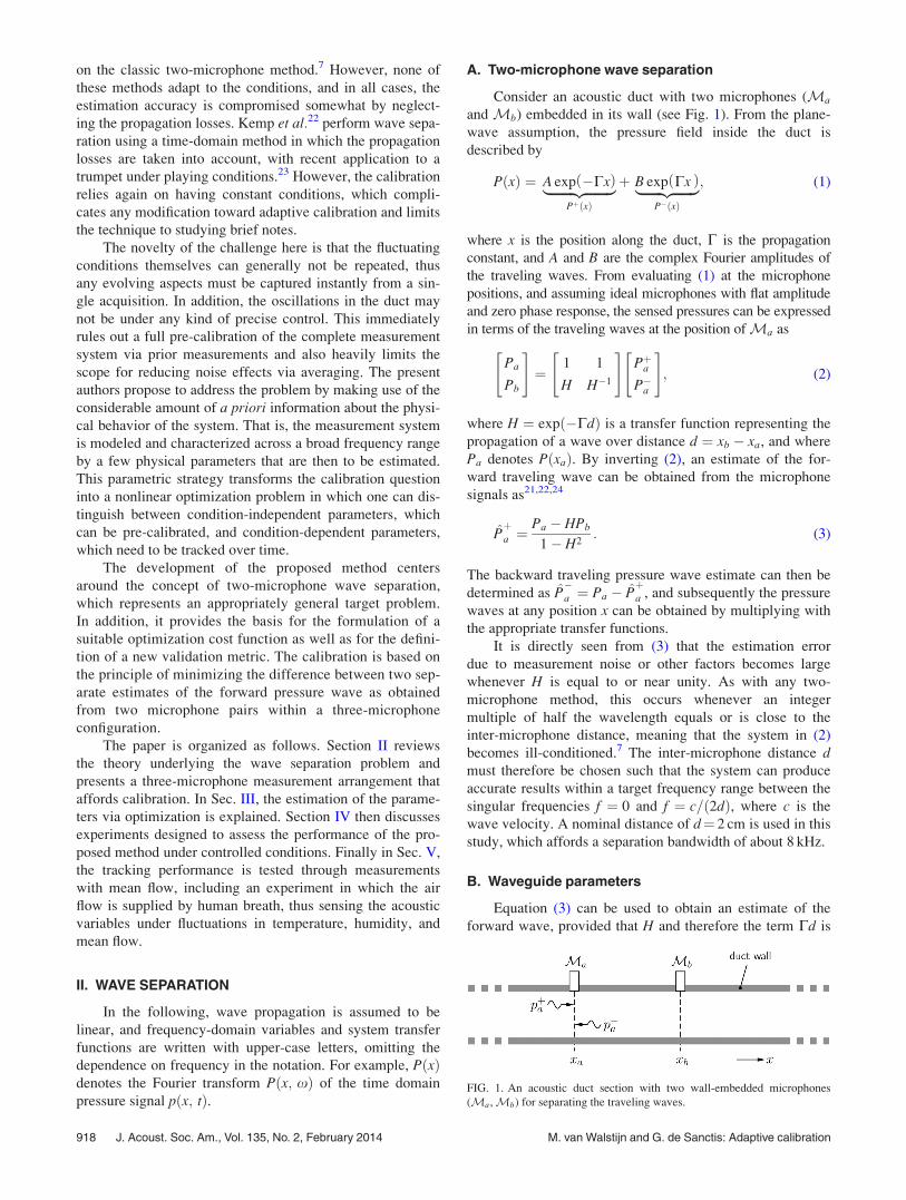
A. Two-microphone wave separation

Consider an acoustic duct with two microphones (Ma

andMb) embedded in its wall (see Fig. 1). From the plane-

wave assumption, the pressure field inside the duct is

described by

PðxÞ ¼ A exp �Cxð Þ|fflfflfflfflfflfflfflffl{zfflfflfflfflfflfflfflffl}PþðxÞ

þ B exp Cxð Þ|fflfflfflfflfflfflffl{zfflfflfflfflfflfflffl}P�ðxÞ

; (1)

where x is the position along the duct, C is the propagation

constant, and A and B are the complex Fourier amplitudes of

the traveling waves. From evaluating (1) at the microphone

positions, and assuming ideal microphones with flat amplitude

and zero phase response, the sensed pressures can be expressed

in terms of the traveling waves at the position ofMa as

Pa

Pb

" #¼

1 1

H H�1

" #PþaP�a

" #; (2)

where H ¼ expð�CdÞ is a transfer function representing the

propagation of a wave over distance d ¼ xb � xa, and where

Pa denotes PðxaÞ. By inverting (2), an estimate of the for-

ward traveling wave can be obtained from the microphone

signals as21,22,24

Pþa ¼

Pa � HPb

1� H2: (3)

The backward traveling pressure wave estimate can then be

determined as P�a ¼ Pa � P

þa , and subsequently the pressure

waves at any position x can be obtained by multiplying with

the appropriate transfer functions.

It is directly seen from (3) that the estimation error

due to measurement noise or other factors becomes large

whenever H is equal to or near unity. As with any two-

microphone method, this occurs whenever an integer

multiple of half the wavelength equals or is close to the

inter-microphone distance, meaning that the system in (2)

becomes ill-conditioned.7 The inter-microphone distance dmust therefore be chosen such that the system can produce

accurate results within a target frequency range between the

singular frequencies f ¼ 0 and f ¼ c=ð2dÞ, where c is the

wave velocity. A nominal distance of d¼ 2 cm is used in this

study, which affords a separation bandwidth of about 8 kHz.

B. Waveguide parameters

Equation (3) can be used to obtain an estimate of the

forward wave, provided that H and therefore the term Cd is

FIG. 1. An acoustic duct section with two wall-embedded microphones

(Ma,Mb) for separating the traveling waves.

918 J. Acoust. Soc. Am., Vol. 135, No. 2, February 2014 M. van Walstijn and G. de Sanctis: Adaptive calibration

known. For pressure waves traveling in a cylindrical duct of

sufficient diameter, such that the boundary layers occupy

only a very small fraction of the duct’s cross-sectional area,

the propagation constant is25

C ¼ jxc

� �þ 1þ jð Þ aw; (4)

where aw is the attenuation constant associated with viscous

drag and heat conduction at the duct wall, which depends on

the duct radius a and the frequency x. Using Pierce’s

formula25

aw ¼1

a

ffiffiffiffiffiffiffiffiffiffigx

2qc2

r1þ c� 1

v

� �; (5)

Eq. (4) can be rewritten as15,24

C ¼ 1

cjxþ g

ffiffiffiffiffijx

p� �; (6)

where g is a coefficient that embeds all the losses per unit

length,

g ¼ 1

a

ffiffiffigq

r1þ c� 1

v

� �; (7)

and where g, q, c, and v, respectively, are the shear viscosity,

the air mass density, the ratio of specific heats, and the

square root of the Prandtl number.25,26 The transfer function

may thus be written as a function of just two parameters

ðs; gÞ;

H ¼ exp �s jxþ gffiffiffiffiffijx

p� �h i; (8)

where s ¼ d=c represents the time it takes a lossless wave to

travel over a distance d. Although more refined formulations

of C are possible,26 it can be verified experimentally27 that

(4) is accurate for jCaj < 1.

For estimation under fluctuating conditions, the pres-

ence of a small mean flow in the duct has to be considered,

as is the case when air is blown into the bore of a wind

instrument. This means that the propagation constant takes

on a different form depending on the traveling direction9,11

Cþ ¼ C1þM

; C� ¼ C1�M

; (9)

where M is the mean flow Mach number, and where the

superscripts “þ” and “�” indicate the positive and the nega-

tive traveling direction, respectively. The expressions in (9)

only hold for small Mach numbers (M� 1), in which case

the first-order Taylor approximation ð1þMÞ�1 ’ 1�Mcan be employed in defining the transfer functions represent-

ing wave travel in either direction over a section distance

d ¼ cs;

H6 ¼ exp � s16M

jxþ gffiffiffiffiffijx

p� �� ’ Hð17MÞ; (10)

where, on the right-hand side of (10), H is the inter-

microphone transfer function of section m in the absence of

mean flow as defined by (8).

C. Three-microphone measurement configuration

The waveguide parameters ðs; g; MÞ can be determined

via calibration, but this requires additional information,

which can be obtained by using more than two microphones.

To limit the impact on the system under study, the number

of microphones is kept to three. These are labeledM1,M0,

and M2, and their relative positions along the duct can be

seen in Figs. 2 and 6. The argument for restricting the num-

ber of microphones is particularly strong for wave separation

in musical wind instruments, which generally have limited

space regarding fitting microphones in the wall of any of its

cylindrical bore sections.

The signal path for the pressure waves in the proposed

three-microphone measurement configuration is depicted

schematically in Fig. 2. Each block labeled H6m models

propagation of a pressure wave over an inter-microphone

distance, and the corresponding wave travel times in the

absence of a mean flow are denoted sm (m ¼ 1; 2). To

develop a practical measurement method, the following

non-idealities are taken in account in comparison to the two-

microphone wave separation discussed in Sec. II A. First, the

spacing between the microphones cannot be assumed to pre-

cisely equal the nominal value, thus s1 6¼ s2. Second, charac-

teristics of the microphones and the acquisition system are

accounted for by assigning (frequency-dependent) complex

amplitudes (G1; G0; G2) to the acquisition channels. The

number of additional system parameters to be estimated can

be reduced by treatingM0 as the reference microphone and

defining two inter-channel complex amplitudes,

F1 ¼G1

G0

¼ a1 expð�jxd1TÞ; (11)

F2 ¼G2

G0

¼ a2 expð�jxd2TÞ; (12)

where the frequency-independent constants a1; a2 and

d1; d2, respectively, represent the inter-channel gains and

delays, and T is the sampling period. It is worth emphasizing

that modeling the sensitivity differences between acquisition

FIG. 2. Signal path for the pressure waves inside a duct section with three

microphones. On the input side, s represents the source signal injected into

the duct section, first arriving at M1 as a forward-traveling wave. Each of

the recorded microphone signals si equals the local pressure filtered by the

respective acquisition channel response Gi (i ¼ 1; 0; 2). R represents the

reflection function as seen fromM2.

J. Acoust. Soc. Am., Vol. 135, No. 2, February 2014 M. van Walstijn and G. de Sanctis: Adaptive calibration 919

channels with simple constants does not imply that the

microphones are assumed to have flat frequency responses;

the only requirement is that the microphones have (nearly)

identical characteristics, which tends to be sufficiently met

when they are of the same type. Including the inter-channel

delays is necessary whenever the employed digital acquisi-

tion system uses time-multiplexing (this the case for most

low-cost multi-channel data acquisition systems), resulting

into inter-channel sub-sample delays that need correcting to

avoid estimation errors.

From the signal path in Fig. 2, and considering that

HþH� ¼ H2, the generic two-microphone wave separation

formula that replaces (3) after taking into account a mean

flow and the non-idealities becomes

Pþa ¼

Pa � Hð1þMÞPb

1� H2¼ SaF�1

a � Hð1þMÞSbF�1b

G0 1� H2ð Þ : (13)

D. Frequency domain processing

In principle it is possible to realize Eq. (13) in the time

domain, which amounts to filtering of the discrete-time

microphone signals sa½n� and sb½n�, where n is the time index.

Similar linear filtering operations are required in the parame-

ter estimation methods discussed in Sec. III. The common

element in these signal processing operations is the modeling

of propagation over an inter-microphone distance, which in

the frequency domain is expressed as the multiplication with

a transfer function of the form of (10). Even though accurate

discrete-time formulations are possible,28,29 this invariably

involves elaborate filter coefficient calculations for which

closed-form expressions are generally not available. Hence

time-domain processing would significantly complicate the

calibration procedure as well as put limitations on it regard-

ing the use of analytical gradient methods. For this reason,

the proposed algorithms largely operate in the frequency

domain, allowing direct evaluation of H in its simple ana-

lytic frequency-domain form.

To obtain the Fourier transforms of the acquired micro-

phone signals, the discrete Fourier transform (DFT) is used.

Wave separation is performed on the resultant discrete spec-

tra by first evaluating (8) and then applying (3), after which

an inverse DFT is used to transform back to the time domain.

Linear-phase post-process filtering is applied to remove any

frequency components around and above the first singular

frequency as well as any components at and near frequency

zero. In the parameter estimation procedure, a smooth analy-

sis window is applied before taking a DFT to reduce spectral

leakage. Throughout the manuscript, presented simulation

and measurement results are obtained using a 100 kHz sam-

pling frequency. The analysis window length is 8192 sam-

ples unless stated differently.

E. Calibration and tracking

The calibration problem to be addressed can now be

stated as the estimation of eight system parameters, which,

grouped into a vector, are

v ¼ s1; r; g; a1; a2; d1; d2; M½ �; (14)

where r ¼ s2=s1 is the propagation time ratio. Before discus-

sing how to best estimate v, it is important to note that is not

possible to estimate the entire parameter vector using a sole

acquisition of microphone signals. This is because the effect

that the inter-channel delays have on the system is equivalent

and directly interchangeable to that of the mean flow, so the

problem would be underdetermined. Therefore a distinction

is made between tracking parameters and structural parame-

ters. The latter category includes the propagation time ratio

and the inter-channel gains and delays; these parameters can

be considered as independent of mean flow, temperature,

and humidity provided that sufficiently condition-proof sen-

sors are employed. The parameters that, under time-varying

conditions, are to be tracked are s1, g, and M; the parameter

s2 can be determined subsequently as s2 ¼ rs1. For valida-

tion purposes, the methodology is first tested in Sec. IV for

controlled, constant conditions without mean flow (thus

setting M ¼ 0) in which case the estimation of seven param-

eters can be achieved from a single acquisition.

III. PARAMETER ESTIMATION

A. Equation error cost function

The information embedded in the three microphone

signals can be used to estimate the parameters via optimiza-

tion, which requires the definition of an error and associated

cost function. To this purpose, consider employing (13) with

two different microphone pairs (M1, M0) and (M1, M2),

resulting into two separate estimates of the forward traveling

wave at the position ofM1,

Pþ1 j10 ¼

P1 � Hð1þMÞ1 P0

1� H21

; (15)

Pþ1 j12 ¼

P1 � Hð1þMÞ1 H

ð1þMÞ2 P2

1� H21H2

2

: (16)

At first sight, it may seem that simply squaring the estimator

difference Pþ1 j10 � P

þ1 j12 and summing over a range of

frequencies would give a suitable cost function to be mini-

mized. However, because of the system poles (the denominator

roots), such a cost function is characterized by many local min-

ima. A similar issue arises in adaptive filter theory in which

evaluating the estimator difference would amount to a recur-

sive filtering operation. A common way to address this prob-

lem is to break the recursion by replacing the feedback to the

estimated filter with the reference signal, which leads to the

so-called equation error method.30 For the problem at hand, an

equation error can be obtained by multiplying the estimator

difference with 1� H21

�1� H2

1H22

�H�ð1þMÞ1 , which yields

E0 ¼Hð1�MÞ1 1� H2

2

�P1 þ H2

1H22 � 1

�P0

þ Hð1þMÞ2 1� H2

1

�P2; (17)

or, in terms of the microphone signals, after multiplying

with F1F2,

920 J. Acoust. Soc. Am., Vol. 135, No. 2, February 2014 M. van Walstijn and G. de Sanctis: Adaptive calibration

E ¼Hð1�MÞ1 1�H2

2

�F2S1 þ H2

1H22 � 1

�F1F2S0

þHð1þMÞ2 1�H2

1

�F1S2: (18)

For an idealized system, in which F1 ¼ F2 ¼ M ¼ 0 and

H1 ¼ H2, Eq. (18) reduces to a preliminary formulation,15

which uses the more intuitive definition of the error as the

difference between the pressure directly measured at the

central microphone and an estimate of it calculated from P1

and P2.

A cost function that can be applied to a set of micro-

phone signals of finite length N sampled at a rate fs ¼ 1=Tcan thus be obtained by evaluating the equation error spec-

trum at a selected set of frequencies of interest,

nðvÞ ¼Xk¼k2

k¼k1

jE½k�j2; (19)

where E½k� denotes the kth component of the equation error

spectrum, corresponding to the frequency fk ¼ kfs=N. Where

needed, the immunity to noise can be improved by evaluat-

ing the power spectrum jEj2 using Welch’s method,31 which

averages over a successive set of overlapping windowed

data sub-segments, at the price of a reduced resolution in

either frequency or time.

It is worthwhile noting that the bandwidth restriction

on the wave separation due to singularities mentioned in

Sec. II A does not apply to the parameter estimation proce-

dure. That is, the fact that the term jE½k�j2 drops toward zero

at singular frequencies does not have a detrimental effect on

the estimation, so a wider range of frequencies can be used.

The estimation bandwidth is constrained, however, by the

plane-wave assumption, which holds up to about the upper-

limit frequency,11

fu ¼1:84c

ffiffiffiffiffiffiffiffiffiffiffiffiffiffiffi1�M2p

2pa: (20)

B. Optimization

The estimation problem can now be defined as finding

the optimum vector v of Q parameters that minimizes the

cost function

v ¼ argminv2RQ

nðvÞ�

: (21)

This is a nonlinear optimization problem that can be solved

using standard iterative methods, provided that convergence

to local minima can be avoided. A practical way to investi-

gate the search space is through the use of acquisition data

generated with simulations of the system in Fig. 2. For

example, Fig. 3 shows n as a function of s1 and s2, as eval-

uated via simulations for a white Gaussian noise source. For

Fig. 3(a), the sum in (19) is limited between 0 and 8 kHz,

while for Fig. 3(b), it is limited between 0 and 16 kHz. The

parameter values used in the simulations are: s1 ¼ s2 ¼ s0

¼ 0.05826, g ¼ g0 ¼ 0:76 Hz12, a1 ¼ a2 ¼ 1, d1 ¼ d2 ¼ 0,

and M ¼ 0. The nominal values s0 and g0 were calculated

from air constants as predicted by theory26 for the room

temperature recorded during the validation experiments

described in Sec. IV and assuming the inter-microphone dis-

tances to equal the nominal value d ¼ 2 cm. In evaluating

the cost function, all parameters apart from s1 and s2 were

set at the nominal theory values used in the simulation.

As can be seen from the contour plots in Fig. 3, the cost

function may contain several local minima. However, good

initial guesses of most of the parameters are available; in

particular, the values of s1, s2, and g are approximately

known from theory. This makes the optimization problem

tractable with the use of local (unconstrained) minimization

methods.32 The Nelder–Mead simplex method33 converges

sufficiently fast in this case and is used for all results

presented here. Alternatively, better convergence may be

obtained using gradient-based methods. More specifically,

because of the frequency-domain formulation, it is possible

to obtain analytical expressions of the first and second order

derivatives of the cost function24 and thus the Hessian matrix

of n, which enables (21) to be solved using for example

Newton’s method.32

Comparing the two contour plots shows that the basins

of convergence become smaller when a larger frequency

FIG. 3. Contour plots of n as a function of s1 and s2 as evaluated for fre-

quencies up to 8 kHz (a) and 16 kHz (b). The physically correct target mini-

mum lies at coordinates ð1; 1Þ.

J. Acoust. Soc. Am., Vol. 135, No. 2, February 2014 M. van Walstijn and G. de Sanctis: Adaptive calibration 921

range is used in (19). This means that the concavity of the

basin around the optimum is more pronounced for a larger

bandwidth, which, in the presence of extraneous measure-

ment noise, leads to a smaller variance in the estimate.

Hence if needed, it can be ensured that the initial guess falls

into the correct basin by first estimating on a smaller fre-

quency range, after which the estimate can be improved with

a second estimation on a larger frequency range.

Further simulations, the results of which are omitted

here for brevity, show that the cost function is similarly

dependent on the channel amplitudes (a1; a2Þ but in compar-

ison is considerably less sensitive to changes in the parame-

ters g, d1, d2, and M. These smaller dependencies imply that

accurate measurements in g or M are possible only when all

the parameters are estimated with high accuracy. This sug-

gests that, for example, the measurement of M can in itself

be used as a way of assessing the validity and accuracy of

the estimation procedure. Hence for experiments in which

no direct separation reference measure is available, such as

those discussed in Sec. V, wave separation may be studied

and assessed indirectly through Mach number estimations.

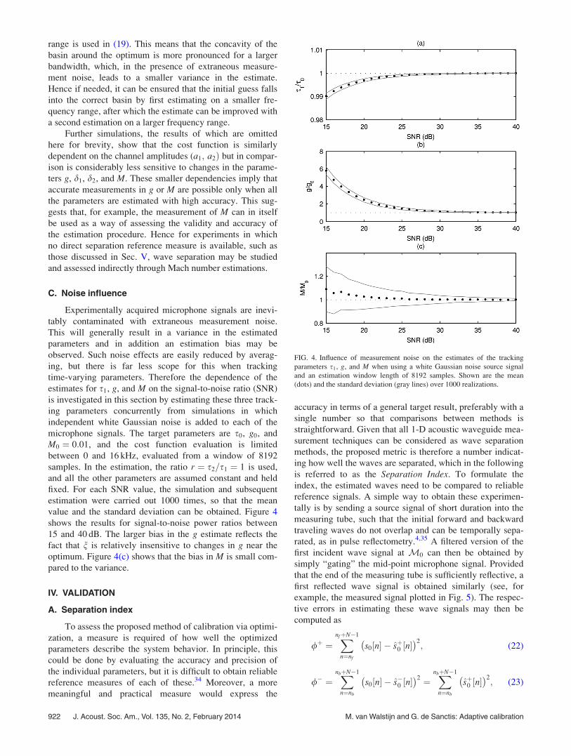
C. Noise influence

Experimentally acquired microphone signals are inevi-

tably contaminated with extraneous measurement noise.

This will generally result in a variance in the estimated

parameters and in addition an estimation bias may be

observed. Such noise effects are easily reduced by averag-

ing, but there is far less scope for this when tracking

time-varying parameters. Therefore the dependence of the

estimates for s1, g, and M on the signal-to-noise ratio (SNR)

is investigated in this section by estimating these three track-

ing parameters concurrently from simulations in which

independent white Gaussian noise is added to each of the

microphone signals. The target parameters are s0, g0, and

M0 ¼ 0:01, and the cost function evaluation is limited

between 0 and 16 kHz, evaluated from a window of 8192

samples. In the estimation, the ratio r ¼ s2=s1 ¼ 1 is used,

and all the other parameters are assumed constant and held

fixed. For each SNR value, the simulation and subsequent

estimation were carried out 1000 times, so that the mean

value and the standard deviation can be obtained. Figure 4

shows the results for signal-to-noise power ratios between

15 and 40 dB. The larger bias in the g estimate reflects the

fact that n is relatively insensitive to changes in g near the

optimum. Figure 4(c) shows that the bias in M is small com-

pared to the variance.

IV. VALIDATION

A. Separation index

To assess the proposed method of calibration via optimi-

zation, a measure is required of how well the optimized

parameters describe the system behavior. In principle, this

could be done by evaluating the accuracy and precision of

the individual parameters, but it is difficult to obtain reliable

reference measures of each of these.34 Moreover, a more

meaningful and practical measure would express the

accuracy in terms of a general target result, preferably with a

single number so that comparisons between methods is

straightforward. Given that all 1-D acoustic waveguide mea-

surement techniques can be considered as wave separation

methods, the proposed metric is therefore a number indicat-

ing how well the waves are separated, which in the following

is referred to as the Separation Index. To formulate the

index, the estimated waves need to be compared to reliable

reference signals. A simple way to obtain these experimen-

tally is by sending a source signal of short duration into the

measuring tube, such that the initial forward and backward

traveling waves do not overlap and can be temporally sepa-

rated, as in pulse reflectometry.4,35 A filtered version of the

first incident wave signal at M0 can then be obtained by

simply “gating” the mid-point microphone signal. Provided

that the end of the measuring tube is sufficiently reflective, a

first reflected wave signal is obtained similarly (see, for

example, the measured signal plotted in Fig. 5). The respec-

tive errors in estimating these wave signals may then be

computed as

/þ ¼XnfþN�1

n¼nf

s0½n� � sþ0 ½n� �2

; (22)

/� ¼XnbþN�1

n¼nb

s0½n� � s�0 ½n� �2 ¼

XnbþN�1

n¼nb

sþ0 ½n� �2

; (23)

FIG. 4. Influence of measurement noise on the estimates of the tracking

parameters s1, g, and M when using a white Gaussian noise source signal

and an estimation window length of 8192 samples. Shown are the mean

(dots) and the standard deviation (gray lines) over 1000 realizations.

922 J. Acoust. Soc. Am., Vol. 135, No. 2, February 2014 M. van Walstijn and G. de Sanctis: Adaptive calibration

where sþ0 ½n� and s�0 ½n�, respectively, are the estimated

forward and backward waves, both filtered by the channel

response G0. The time windows ½nf ; nf þ N � 1� and

½nb; nb þ N � 1� are chosen such that the compact forward

and backward wave signals are cleanly captured from the

mid-point microphone signal. However, neither /þ nor /�

can by itself serve as an adequate measure because a null

error would result whenever s6;0 � s0, a situation that can

occur for some choices of the parameters not corresponding

to separating the waves. In addition, both error terms are pro-

portional to the amplitude of the acquired signals. It follows

that what should be measured is the sum of the normalized

errors in the reconstructions of the incident and reflected

waves,

/ ¼ /þ

gþþ /�

g�; (24)

where

gþ ¼XnfþN�1

n¼nf

s20½n�; g� ¼

XnbþN�1

n¼nb

s20½n� (25)

are the respective normalizing energies. However, depending

on the spectral content of the source signal, this measure

may not be significant at all frequencies. The performance of

a separation algorithm is therefore generally best studied

within a specified bandwidth, for which (24) is re-written in

a frequency-dependent form

U½k� ¼jS0;f ½k� � S

þ0;f ½k�j

2

NgþþjSþ0;b½k�j

2

Ng�; (26)

where S0;f and Sþ0;f are the DFTs of, respectively, s0½n� and

sþ0 ½n� for nf � n < nf þ N, and Sþ0;b is the DFT of sþ0 ½n� for

nb � n < nb þ N. The separation index for a specified band-

width ranging between frequencies indexed by k1 and k2 can

then be defined in decibels as

W ¼ 10 log10

Xk2

k¼k1

U½k�

0@

1A: (27)

Note that for the calculation of W, only the forward wave

estimate Sþ0 is required; this can be calculated from (13) for

the microphone pair (M0,M2) with M ¼ 0 as

Sþ0 ¼ G0P

þ0 ¼

S0 � ðH˚2=F˚ 2ÞS2

1� H2˚2

; (28)

where H˚2 is the transfer function H2 evaluated with the opti-

mum parameter vector v and F˚ 2 is the corresponding inter-

channel complex amplitude ofM2.

B. Measurement apparatus and procedure

The measurement apparatus used in the validation

experiments is shown schematically in Fig. 6. Endevco

piezo-resistive microphones (model 85070C-1) and a JBL

compression driver (model 2426J) are used to, respectively,

sense and drive the acoustic field, while a National

Instruments USB-6251 acquisition board is employed for

digital-to-analog conversion to 16-bit signals at a 100 kHz

sample rate. A metal cap is placed at the end of the meas-

uring tube to maximize reflections.

Two acquisitions are carried out, one for pre-calibration

and one for testing wave separation for a specific test signal.

In the pre-calibration acquisition, the maximum-length

sequence (MLS) method36 is used to measure the impulse

responses at the microphone positions. A 19th-order MLS is

sent to the compression driver and the signals from the three

microphones acquired. Next, the cross-correlation between

the MLS input signal and each of the three acquired micro-

phone signals is computed; this yields three impulse

responses, the spectra of which are used as S1, S0, and S2 in

the algorithm for estimating the system parameters as

explained in Sec. III. In the second acquisition, a test signal

of short duration is fed to the compression driver, for exam-

ple a Hanning-windowed sine wave. Averaging the micro-

phone signals over multiple acquisitions can be used to

improve the SNR. Figure 5 shows the first 1400 samples of

the signal obtained by averaging over 100 acquisitions at

M0 for a short windowed sine wave source signal. For com-

parison, the estimated forward wave signal calculated with

(28) after calibration via optimization is also plotted; this

demonstrates the cancellation of the backward-traveling

wave. As explained in Sec. IV A, the actual forward travel-

ing wave signal can in this case be extracted from the

acquired microphone signal by gating.

FIG. 5. Acquired signal atM0 after averaging over 100 acquisitions with a

windowed 3 kHz sine wave source signal. The forward wave estimate

obtained with (28) is also shown.

FIG. 6. Measurement apparatus used in the validation experiments. The in-

ternal diameter of the cylindrical measuring tube is 12.7 mm, and the micro-

phone diameter is 2.5 mm.

J. Acoust. Soc. Am., Vol. 135, No. 2, February 2014 M. van Walstijn and G. de Sanctis: Adaptive calibration 923

C. Reference experiment

For constant propagation conditions, the measurement sys-

tem can also be calibrated through pre-measured responses. The

estimated forward wave thus obtained can be used as a refer-

ence, by separation index comparison. Referring again to Fig. 2,

the signals s0 and s2 acquired by microphonesM0 andM2 can

be written as a function of the forward pressure wave at M0.

Again taking M ¼ 0, the frequency-domain relationships are

S0 ¼ G0 1þ H22R

�Pþ0 ; (29)

S2 ¼ G2 H2 þ H2Rð ÞPþ0 : (30)

By writing the forward and the backward traveling wave

components separately,

S0;f ¼ G0Pþ0 ; S0;b ¼ G0H22RPþ0 ; (31)

S2;f ¼ G2H2Pþ0 ; S2;b ¼ G2H2RPþ0 ; (32)

the following transfer functions can be defined:

S2;f

S0;f¼ G2

G0

H2 ¼ H02;S0;b

S2;b¼ G0

G2

H2 ¼ H002 : (33)

This implies that H2 ¼ffiffiffiffiffiffiffiffiffiffiffiffiH02H002

p, and that, analogous to (28),

an estimate of the (filtered) forward wave is

Sþ0 ¼

S0 � H002 S2

1� H02H002: (34)

Measures of H02 and H002 can be evaluated from (33) after

extracting the relevant forward and backward waves from

the same pre-calibration acquisition as used for the optimiza-

tion. That is, S0;f and S2;f are obtained by isolating the first

forward wave from each of the respective impulse responses

measured using the MLS method as explained in Sec. IV B

and taking the DFTs after zero-padding from 512 to 8192

samples. The transfer function H02 is then calculated by

dividing these spectra. The second transfer function H002 is

determined in the same fashion, where S2;b and S0;b are the

DFTs of the signals obtained by isolating the first end-

reflection in each of the two measured impulse responses.

D. Results

The proposed method of calibration via optimization is

compared in this section to results obtained with the

reference experiment. To get further insight into the effect of

the calibration on W, a third estimate is calculated in which

the transfer function is evaluated from theory, thus applying

(28) but with F˚ 2 and H˚2, respectively, replaced by 1 and H0,

the latter being the transfer function evaluated using the

nominal theory parameters as used for the simulated cost

function results in Sec. III B.

Table I lists the separation index results for two different

test signals, a white Gaussian noise and a 3 kHz sine wave,

both windowed with a 256-sample length Hanning window.

For the white Gaussian noise, the sum in (27) is evaluated

for frequencies between 0.1 and 8 kHz, while for the 3 kHz

sine wave, the used limits are 2 and 4 kHz. The results are

obtained from a single acquisition as well as by averaging

over 16 and 100 acquisitions. Figure 7 shows the separation

index as a function of frequency. As can be expected, the

results significantly improve with averaging. More impor-

tantly, they demonstrate that (1) calibration generally

improves the estimation in comparison to using theoretical

parameter values and (2) the optimization method gives

results similar to those obtained with the reference experi-

ment. Note that the results obtained with the theoretical pa-

rameters depend on having conditions that allow prediction

from an available temperature measurement; this is generally

not the case in the envisaged scenarios in which any reliance

on theory will thus cause larger wave separation errors.

V. MEASUREMENT WITH MEAN FLOW

In this section, the tracking performance of the proposed

estimation method is investigated by estimating the parame-

ters from microphone acquisitions obtained during a period of

time-varying mean flow through two separate experiments.

A. Dry air with CPU fan flow

For this experiment, the measuring tube is terminated on

one end by a compression driver fed with a white noise

broadband signal. The other end is fitted with a funnel and a

small fan taken from a CPU cooling system (see Fig. 8). An

airhole is placed just before the driver to allow a steady cir-

culation of the air. This arrangement allows generating a

controlled flow while avoiding as much as possible any fur-

ther perturbations in the conditions.

The experiment consists in the acquisition of two

sequences; the first, with the fan switched off, is used to pre-

calibrate the system, estimating “zero-flow values” of the

first seven parameters of the vector in (14). In the second

TABLE I. Separation index results (in dB).

White Gaussian noise 3 kHz sine wave

Averaging: 1 16 100 1 16 100

Theory Sþ0 ¼

S0 � H0S2

1� H20

�19.2 �25.2 �25.2 �31.8 �31.9 �32.0

Reference Sþ0 ¼

S0 � H002 S2

1� H02H002�20.7 �34.2 �37.9 �43.2 �49.4 �50.0

Optimization Sþ0 ¼

S0 � ðH˚2=F˚

2ÞS2

1� H2˚2

�21.7 �34.7 �39.1 �46.3 �48.3 �49.8

924 J. Acoust. Soc. Am., Vol. 135, No. 2, February 2014 M. van Walstijn and G. de Sanctis: Adaptive calibration

experiment, the fan is first switched on, left to run for a few

seconds, and then switched off. The expected result is thus a

non-negative flow velocity that builds up from zero to a

steady level and then decays back to zero during the free-

rotating period in which the fan loses its kinetic energy.

Because the parameters d1 and d2 directly affect the

flow velocity estimate, they must be estimated from the pre-

calibration acquisition and kept fixed in the second acquisi-

tion. Block-wise estimation from the second acquisition is

then performed in two different ways, first by estimating all

the remaining six parameters, and second by keeping r, a1,

and a2 fixed, thus estimating only the waveguide parameters

s1, g, and M. This allows verifying to what extent the

assumption that only the latter vary with the conditions

holds. The resulting evolutions in s1, g, and M are shown in

Fig. 9 and indicate that not only M but also s1 and s2 are

time-varying in this case, while g mainly shows a statistical

variation around its mean; the latter trend was also observed

in the other parameters estimated (r; a1; a2), although with

considerably smaller variance. Figure 9(c) confirms for this

case that it is reasonable to assume that all system parame-

ters apart from s1, s2, and M are constant. Furthermore, the

mean flow velocity (v ¼ Mc) follows the expected trend:

The null flow is correctly estimated, a steady state period

can be observed, and even the first-order response of the fan

motor to the voltage step is visible. The small step in s1 at

t¼ 1.2 s suggests a change in the wave speed corresponding

to a temperature drop of about 1.1 �C, a possible explanation

of which is that the introduction of a mean flow may cause a

change in the heat transfer between the air and the tube wall.

B. Flow from breath

Given that the flow velocity estimation in a controlled

environment returns plausible results, the experiment is

repeated but with the funnel and fan replaced with a (reed-

less) clarinet mouthpiece and supplying an airflow by a

human blowing moist air into the measuring tube; this pro-

vides conditions similar to those in a wind instrument. By

exclusively exhaling during the acquisition, the mean flow

velocity is again expected to be non-negative. In addition, an

effort was made to generate a monotonic rise and fall in

mean flow. Figure 10 shows the resulting parameterFIG. 8. Experimental setup used for measurements with mean flow. The in-

ternal diameter of the cylindrical measuring tube is 15 mm.

FIG. 9. Evolution of s1, g, and M, as estimated under dry conditions with a

fan generating a mean flow. The estimates were computed every 8192 sam-

ples, using a 16 384-sample analysis window. The legend in (c) indicates

which parameters were estimated.

FIG. 7. Separation index as a function of frequency from 100 averaged

acquisitions for a windowed white Gaussian noise source signal (a) and win-

dowed 3 kHz sine wave (b). Singular frequencies are positioned at 0 and

8.58 kHz.

J. Acoust. Soc. Am., Vol. 135, No. 2, February 2014 M. van Walstijn and G. de Sanctis: Adaptive calibration 925

evolutions, obtained similarly to the experiment with the dry

air flow. The evolution of M is again insensitive to whether

the parameters r, a1, and a2 are estimated or held fixed. A

rigorous analysis of the causes behind the visible fluctuations

in s1 and g is beyond the scope of this study; in particular

the fluctuations in g may be due to many different factors

and show no consistency between the two estimations. One

main trend that proved consistent across all measurements of

this type can be explained though. That is, the significant

drop in s1 at the point where the mean flow starts to rise

marks the arrival of air of higher temperature and humidity,

causing a sudden increase in wave speed.

Figure 10(c) also shows an additional estimation from

the same data in which all parameters except M are held

fixed. This results into an erratic, non-smooth flow evolution,

and even results into a period of negative estimated flow,

which is not consistent with the applied input. This result

exemplifies the notion that under transient propagation con-

ditions, the system calibration must be adaptive in its time-

variant parameters.

VI. CONCLUDING REMARKS

The problem of calibrating two-microphone wave

separation methods under time-varying conditions can be

made tractable by physical parameterization of the inter-

microphone propagation transfer function. It has been shown

that a three-microphone measurement configuration can be

used to calibrate and track the relevant parameters. For meas-

urements under constant conditions, the proposed method of

calibration via optimization has been shown in Sec. IV to per-

form very similarly to a more standard calibration method

based on pre-measuring system responses. This result vali-

dates the basic methodology; in particular, it justifies the way

in which the three-microphone measurement system has been

parameterized in Sec. II C. The measurements with mean

flow in Sec. V demonstrate that adaptive calibration is not

only possible but indeed necessary when several condition

aspects, such as temperature and humidity, are variable.

Although the estimated Mach numbers are not directly com-

pared to a reference measure, the observed mean flow evolu-

tions are plausible and consistent with the applied inputs.

These results pave the way for addressing a range of

challenging measurement problems. Of particular interest to

the authors is the determination of the acoustic variables

inside a wind instrument under playing conditions in a non-

intrusive manner in the sense that there is minimal interfer-

ence with the normal functioning and musician’s control of

the instrument. The proposed methodology has in fact al-

ready been successfully employed as such, in the form of

wave separation in a simplified clarinet for the purpose of

estimating the reed parameters by inverse modeling.17

Although wave propagation in an instrument bore may

become non-linear at high playing levels,37 this would not

invalidate the basic two-microphone wave separation

method because such effects are small over short distances,

thus allowing for a locally linear approximation.21

The approach taken in the present study may also lend

itself to improvements and extensions in other applications.

For example, a more accurate impedance measurement in the

presence of a mean flow may be possible if the Mach number

is included in the calibration procedure.10 Generally, not

requiring any additional measurements with special made-to-

precision objects may represent a significant advantage in

certain measurement scenarios. Finally, the ability of cali-

brating in-system on short signals could also be useful in con-

trol applications given that the existing control methods

usually achieve the required efficiency and noise immunity at

the cost of reducing the wave separation accuracy.

ACKNOWLEDGMENTS

The research was supported by the Engineering and

Physical Sciences Research Council (UK), Grant No

EP/D074983/1. The authors are grateful to David Sharp for

his helpful comments on earlier versions of this text.

1R. Causse, J. Kergomard, and X. Lurton, “Input impedance of brass musi-

cal instruments—comparison between experiment and numerical models,”

J. Acoust. Soc. Am. 75, 241–254 (1984).2V. Gibiat and F. Laloe, “Acoustical impedance measurements by the two-

microphone-three-calibration (TMTC) method,” J. Acoust. Soc. Am. 88,

2533–2545 (1990).3N. Amir, U. Shimony, and G. Rosenhouse, “A discrete model for tubular

acoustic systems with varying cross-section the direct and inverse prob-

lems. Part 2: Experiments,” Acta Acust. Acust. 81, 463–474 (1995).

FIG. 10. Evolution of s1, g, and M, as estimated under fluctuations in

temperature and humidity effected by blowing into the measuring tube.

The estimates were computed every 8192 samples, using a 16 384-sample

analysis window. The legend in (c) indicates which parameters were

estimated.

926 J. Acoust. Soc. Am., Vol. 135, No. 2, February 2014 M. van Walstijn and G. de Sanctis: Adaptive calibration

4D. B. Sharp, “Acoustic pulse reflectometry for the measurement of musi-

cal wind instruments,” Ph.D. thesis, University of Edinburgh, 1996,

pp. 1–192.5J.-P. Dalmont, C. J. Nederveen, V. Dubos, S. Ollivier, V. Meserette, and

E. te Sligte, “Experimental determination of the equivalent circuit of an

open side hole: Linear and non linear behaviour,” Acta Acust. Acust. 88,

567–575 (2002).6S. Rodriguez, V. Gibiat, A. Lefebvre, and S. Guilain, “The three-

measurement two-calibration method for measuring the transfer matrix,”

J. Acoust. Soc. Am. 129, 3056–3067 (2011).7A. F. Seybert and D. F. Ross, “Experimental determination of acoustic

properties using a two-microphone random-excitation technique,”

J. Acoust. Soc. Am. 61, 1362–1370 (1977).8M. Abom and H. Boden, “Error analysis of two–microphone measure-

ments in ducts with flow,” J. Acoust. Soc. Am. 83, 2429–2438 (1988).9S.-H. Jang and J.-G. Ih, “On the multiple microphone method for meas-

uring in-duct acoustic properties in the presence of mean flow,” J. Acoust.

Soc. Am. 103, 1520–1526 (1998).10S. Rodriguez, V. Gibiat, A. Lefebvre, and S. Guilain, “Input impedance in

flow ducts: Theory and measurement,” J. Acoust. Soc. Am. 132,

1494–1501 (2012).11Y.-B. Kim and Y.-H. Kim, “A measurement method of the flow rate in a

pipe using a microphone array,” J. Acoust. Soc. Am. 112, 856–865 (2002).12P. Dickens, J. Smith, and J. Wolfe, “Improved precision in measurements

of acoustic impedance spectra using resonance-free calibration loads and

controlled error distribution,” J. Acoust. Soc. Am. 121, 1471–1481 (2007).13A. H. Benade and M. I. Ibisi, “Survey of impedance methods and a new

piezo-disk-driven impedance head for air columns,” J. Acoust. Soc. Am.

81, 1152–1167 (1987).14J.-P. Dalmont, “Acoustic impedance measurement. Part I: A review,”

J. Sound Vib. 243, 427–439 (2001).15M. van Walstijn and G. de Sanctis, “Towards physics-based re-synthesis

of woodwind tones,” in International Congress on Acoustics (ICA 2007),Madrid, Spain (2007).

16T. Smyth and J. S. Abel, “Toward an estimation of the clarinet reed pulse

from instrument performance,” J. Acoust. Soc. Am. 131, 4799–4810 (2012).17V. Chatziioannou and M. van Walstijn, “Estimation of clarinet reed

parameters by inverse modelling,” Acta Acust. Acust. 98, 629–639 (2012).18J. Gu�erard and X. Boutillon, “Real time acoustic travelling waves separa-

tion in a tube,” in Proceedings of the 1997 International Symposium onMusical Acoustics, Edinburgh (1997).

19J. Gu�erard, “Numerical modeling and experimental simulation of acoustic

systems: Application to musical instruments” (in French), Ph.D. thesis,

Universit�e de Paris VI, Paris, France, 1998, Chap. 4.20P. Naucl�er and T. S€oderstr€om, “Separation of waves governed by the one-

dimensional wave equation: A stochastic systems approach,” Mech. Syst.

Sig. Proc. 23, 823–844 (2009).

21P. L. Rend�on, F. Ordu~na-Bustamante, D. Narezo, A. P�erez-L�opez, and J.

Sorrentini, “Nonlinear progressive waves in a slide trombone resonator,”

J. Acoust. Soc. Am. 127, 1096–1103 (2010).22J. A. Kemp, M. van Walstijn, D. M. Campbell, J. P. Chick, and R. A.

Smith, “Time domain wave separation using multiple microphones,”

J. Acoust. Soc. Am. 128, 195–205 (2010).23J. A. Kemp, S. Bilbao, J. McMaster, and R. A. Smith, “Wave separation

in the trumpet under playing conditions and comparison with time

domain finite difference simulation,” J. Acoust. Soc. Am. 134,

1395–1406 (2013).24G. de Sanctis and M. van Walstijn, “A frequency domain algorithm for

wave separation,” in 12th International Conference on Digital AudioEffects (DAFx-09), Como, Italy (2009), pp. 498–505.

25A. D. Pierce, Acoustics: An Introduction to Its Physical Principles andApplications (AIP, New York, 1989), Chap. 10.

26D. H. Keefe, “Acoustical wave propagation in cylindrical ducts:

Transmission line parameter approximations for isothermal and noniso-

thermal boundary conditions,” J. Acoust. Soc. Am. 75, 58–62 (1984).27M. van Walstijn, D. Campbell, J. Kemp, and D. Sharp, “Wideband

measurement of the acoustic impedance of tubular objects,” Acta Acust.

Acust. 91, 590–604 (2005).28T. H�elie and D. Matignon, “Diffusive representations for the analysis and

simulation of flared acoustic pipes with visco-thermal losses,” Math.

Models Methods Appl. Sci. 16, 503–536 (2006).29G. De Sanctis, “In-system parametric calibration for two-microphone

wave separation in acoustic waveguides,” Ph.D. thesis, Queen’s

University Belfast, Belfast, U.K., 2012, Chap. 2.30G. C. Goodwin and K. S. Sin, Adaptive Filtering Prediction and Control

(Prentice-Hall, Englewood Cliffs, NJ, 1984), Chap. 3.31P. Welch, “The use of fast Fourier transform for the estimation of power

spectra: A method based on time averaging over short, modified perio-

dograms,” IEEE Trans. Audio Electroacoust. 15, 70–73 (1967).32A. R. Conn, N. I. M. Gould, and P. L. Toint, Trust-Region Methods

(Society for Industrial and Applied Mathematics, Philadelphia, PA, 2000),

Chap. 6.33J. A. Nelder and R. Mead, “A simplex method for function minimization,”

Comput. J. 7, 308–313 (1965).34G. de Sanctis and M. van Walstijn, “Calibration of apparatus for wave

separation in wind instruments,” J. Acoust. Soc. Am. 123, 3016 (2008).35L. Sun and H. Hou, “Transmission loss measurement of acoustic material

using time-domain pulse-separation method (L),” J. Acoust. Soc. Am.

129, 1681–1684 (2011).36J. B. Borish and J. Angell, “An efficient algorithm for measuring the

impulse response using pseudorandom noise,” J. Audio Eng. Soc. 31,

478–488 (1983).37A. Hirschberg, J. Gilbert, R. Msallam, and A. P. J. Wijnands, “Shock

waves in trombones,” J. Acoust. Soc. Am. 99, 1754–1758 (1996).

J. Acoust. Soc. Am., Vol. 135, No. 2, February 2014 M. van Walstijn and G. de Sanctis: Adaptive calibration 927