--

.--

AD-A243 493 QINCIPIENT FAULT DETECTION fUSINGCHIGHER-ORDER

STATISTICS C

APPROVED BYSUPERVISORY COMMITTEE:

Art,

91-17896

91 ! 150

form AApproved

REPORT DOCUMENTATION PAGE oME No A .,o4 8d

1. AGENCY USE ONLY (Lt'e ban ) I2. REPORT DATE 3. REPORT TYPE AND DATES COVERED1.AGNC UEONY Lev bant)T August 1991 RIMJDISSERTATION

4. TITLE AND SUBTITLE 5. FUNDING NUMBERS

Incipient Fault Detection Using Higher-Order Statistics

6. AUTHOR(S)

Richard William Barker, Major

7. PERFORMING ORGANIZATION NAME(S) AND ADDRESS(ES) 8. PERFORMING ORGANIZATIONREPORT NUMBER

AFIT Student Attending: University of Texas AFIT/CI/CIA-91-023D

9. SPONSORING MONITORING AGENCY NAME(S) AND ADDRESS(ES) 10. SPONSORING/MONITORINGAGENCY REPORT NUMBER

AFIT/CI

Wright-Patterson AFB OH 45433-6583

11. SUPPLEMENTARY NOTES

12a. DISTRIBUTION,' AVAILABILITY STATEMENT 12b. DISTRIBUTION CODE

Approved for Public Release lAW 190-1Di.stribl.ted Unlimited

ERNEST A. HAYGOOD, Captain, USAFExecutive Officer

13. ABSTRACT (Maximum 200 wOrds)

14. SUBJECT TERMS 15, NUMBER OF PAGES

17516. PRICE CODE

17. SECURITY CLASSIFICATION 18. SECURITY CLASSIFICATION 19. SECURITY CLASSIFICATION 20. LIMITATION OF ABSTRACTOF REPORT OF THIS PAGE OF ABSTRACT

%5N 750-0--1 2 -5500 S.a-ca-c ;or" 298 kev 2-89)

Copyright

by

Richard William Barker

1991

Dedicated to the Memory of My Dad

Havelock William Barker

' IVq L -

INCIPIENT FAULT DETECTION vAt, i, , . e** _

USING HIGHER-ORDER D i

STATISTICS

by

RICHARD WILLIAM BARKER, B.S., M.B.A., M.S.

DISSERTATION

Presented to the Faculty of the Graduate School of

The University of Texas at Austin

in Partial Fulfillment

of the Requirements

for the Degree of

DOCTOR OF PHILOSOPHY

TIE UNIVFRSITY OF TF.XAS AT \FSTIN

August I9l

Preface

Richard W. BarkerThe University of Texas at Austin, 1991

Supervising Professors: Melvin J. Hinich and Georgia-Ann Klutke

This study balances the development of theory and its application to real

and simulated incipient fault data from systems which have cyclostationary prop-

erties. The study's theoretical contribution reveals the advantages of approaching

estimation of time series in a general framework where estimation of the cumulant

spectrum can reveal implications for three classes of stochastic processes: station-

ary, cyclostationary, and nonstationary. The developed cumulant spectrum esti-

mation capability provides estimates for feature construction in addition to

bispectrum and power spectrum estimates of stochastic process data. Actual ex-

perimental data is obtained to study the incipient wear process of manufacturing

drill bits cutting through epoxy-glass composite material used for construction of

electronic semiconductor panels. The fluctuating vibrations caused by the drill bits

cutting through the epoxy-glass composite are not subject to precise prediction, nor

are the external noise, measurement errors, and other disturbances in the trans-

mission of the vibration signal to three accelerometers mounted on the drilling

machine considered to have tile same characteristic of unpredictability. - Even

though there is some element of determinism in the generated signal data due to the

common periodic excitation of the rotating drill spindle, the vibration signals and

V

noises do vary with time. The randomness which exists from sample function to

sample function throughout a complete ensemble (inherent sampling variability) is

a characteristic of any stochastic process. But there is also a randomness from time

instant to time instant from an object sample function to the same sample function

as the object wears over time. This is the other element of randomness that is of

primary focus in this research. The application portion of the study consists of

pattern recognition analyses of simulated and actual experimental data to determine

the incipient fault discrimination and classification ability of classifiers using fea-

tures with and without higher-order statistical (HOS) information. Exploitation of

probabilistic and statistical concepts has led to a new incipient fault detection ap-

proach for rotating physical systems.

vi

Acknowledgements

First, I thank my wife Judy for all her support and love. I thank Doctor's

Itinich and Klutke, my co-supervising professors, for their guidance, insight, and

encouragement during this conducted research. The dissertation was given a "real

world flavor" with the IBM drill wear application data provided by Dr. Ramirez

and Dr. Thornhill. I thank both of them for their sharing of the data and assistance

in understanding the wear experiment.

vii

INCIPIENT FAULT DETECTION

USING HIGHER-ORDER

STATISTICS

Publication No.

Richard William Barker. Ph.D.The I niversitv of Texas at Austin, 1991

Supervising Professors: Melvin .1. Iinich and Georgia-Ann Klutke

A new analytical approach is developed for detecting incipient faults of

rotating machinery whose periodical characteristics generate time series data repre-

sentable as cyclostationary processes. The new approach is a higher-order statis-

tical (110S) method as nonstationarv time series estimation, in addition to

stationary and nonlinear estimation, provide the basis for enhanced feature infor-

mation of the random fault mechanisms under study. An algorithm selects and

combines different transformed estimates of the raw time series, second-order

cumulant spectrum (nonstationary), power spectrum (stationary), and bispectrum

(nonlinear), for investigation of incipient fault discrimination and classification

power of multivariate classifiers using different extracted feature information sets.

The S110S approach (cumulant spectrum, bispectrum, and power spectrum), is

tested and evaluated against a traditional power spectrum approach with simulated

viii

and actual experimental data. Robustness of the IlOS approach is first investigated

in simulated time series signals with amplitude and phase modulation indices and

differing levels of additive Gaussian noise as parameters. Simulations show that

use of IlOS features improves incipient fault detection capability of a linear

classifier and is less sensitive to Gaussian noise within the signal environment.

Actual vibration signals from a rotating drill wear monitoring study are also ana-

lyzed. The drills are used in the manufacturing of electronic circuit cards from

epoxy-glass composite. Combining HOS features with power spectrum features

improved the overall classification performance of parametric and non-parametric

classifiers. Additionally, the IIOS approach is less sensitive to changes in drilling

process parameters such as circuit card construction and chip load. The pattern

recognition analyses performed in this research provide strong statistical evidence

that HOS estimation and feature extraction is beneficial for discrimination and

classification of incipient failures of rotating tools, a difficult mechanical system

monitoring problem.

ix

Table of Contents

Preface ...................................................... v

Acknowledgements ............................................ vii

Abstract .................................................... viii

List of Tables ................................................ xv

List of Figures .............................................. xvii

Chapter I: Introduction ......................................... I1.1 Introduction .. .. . .. . .. .. . ... . . ... . .. . ... . . ... . .. . .. .. .. . .. 11.2 Problem Statement and Scope ................................. 41.3 General Research Approach and Presentation ..................... 8

Chapter 2: Background ......................................... 92.1 Introduction ............................. ................. 92.2 Existing Incipient Fault Detection Techniques ..................... 92.3 Measuring Differences Among Multivariate Populations ............ 16

2.3.1 Estim ation M ethods .................................... 212.3.1.1 Advantages and Disadvantages of Applied Estimation Methods . 25

2.3.2 Other Estimation Approaches Considered .................... 252.3.3 Mathematical Development of Analysis of Variance ............ 28

2.3.3.1 Partitioning of Variance .............................. 292.3.3.2 One-Way ANOVA and MANOVA ...................... 35

2.3.4 Classifier Performance Measurement Criteria .................. 382.4 Discrimination and Classification of Time Series .................. 402.5 Stochastic Processes and Their Covariance Functions .............. 442.6 Higher-Order Statistical (IIOS) Theory ......................... 48

2.6.1 M oments and Cum ulants ............................ ... 502.6.2 Mathematical Properties of The Bispectrum ................... 532.6.3 Bispectrum-Based Statistical Tests .......................... 592.6.4 Cyclostationary Processes and Iligher-Order Spectra ............ 61

2.7 Sum m ary . .. .. . ... . .. .. .. . ... . .. .. .. .. .. . ... . ... .. . .. .. . 62

Chapter 3: Cumnlant Spectrum Estimation ......................... 643.1 Introduction .............................................. 643.2 Cumulant Spectra and Their Estimation ................. ...... 66

3.2.1 Second-Order Cumulant Spectrum ......................... 683.2.1.1 Principal Domain Development ......................... 733.2.1.2 Estim ation Procedure ................................ 783.2.1.3 Reliability of the Estim ates ............................ 82

X

Chapter 4: HOS Feature Extraction................................ 844.1 Introduction............................................... 844.2 Features and Their Re!ationship to Misclassification Rate ...... 854.3 Existing Feature Extraction Approaches........................... 874.4 New Hybrid Approach....................................... 894.5 Results............................ ...................... 93

Chapter 5: Evaluation of HOS Approach............................ 1095.1 Introduction............................................. 1095.2 Simulated Wear Experiment..................................109

5.2. 1 Experimental Design.................................... 1195.2.2 Results.............................................. 120

5.2.2.1 Discrimination......................................1215.2.2.2 Classification.......................................123

5.3 Actual Wear Experiment Description...........................1265.3.1 Experimental Design.................................... 1285.3.2 Collected Data.........................................1305.3.3 Results.............................................. 134

5.3.3.1 Discrimination......................................1345.3.3.2 Classification.......................................137

Chapter 6: Conclusions and Further Research ........................ 1436.1I Areas of Further Research...... ............................ 1476.2 Summary........................................ ........ 148

Appendices.................................................... 150

Appendix A Second-Order Cumulant Spectrum Estimation Program..........151

Appendix B Harmonic Process Model Stationarity and Finite Memury.........161

Appendix C Power Spectrum Broadening............................. 165

Bibliography................................................... 170

Vita ........................................................ 17;1

x1

List of Tables

Table 4.1: Gaussianity and Linearity Test Statistic Results For New Bits--Actual Wear Experiment ............................... 92

Table 4.2: Gaussianity and Linearity Test Statistic Results For Slightly Used

Bits--Actual Wear Experiment . .......................... 92

Table 4.3: Actual Experiment Feature Extraction--NIP!3 Case ......... 104

Table 4.4: Actual Experiment Feature Extraction--6S2P/3 Case ........ 105

Table 4.5: Actual Experiment Feature Extraction--NIP/4 Case ......... 105

Table 4.6: Actual Experiment Feature Extraction--6S2P/4 Case ........ 106

Table 4.7: Actual Experiment Feature Extraction--Combined Load 3 Case 106

Table 4.8: Actual Experiment Feature Extraction--Combined Load 4 Case 107

Table 4.9: Actual Experiment Feature Extraction--Combined Stack NIPC a se ............................................ 10 7

Table 4.10: Actual Experiment Feature Extraction--Combined Stack 6S2PC a se ............................................ 10 8

Table 5.1: Seven Incipient Fault Detection Scenarios--Simulated Wear Data 115

Table 5.2: Marginal Discrimination Benefit of Combining Power SpectrumWith Second Cumulant Spectrum Features--Simulated Wear Data 121

Table 5.3: Marginal Discrimination Benefit for Combining Bispectrum andSecond-order Cumulant Spectrum with Power SpectrumFeatures--Simulated W ear Data . ........................ 122

Table 5.4: Training Classification Performance of I IOS Features versusPower Spectrum Features--Simulated Wear Data ........... 123

[able 5.5: Second-order Cumulant Spectra & Power Spectra vs PowerSpectra Feature Extraction Test Classification--Simulated WearD a ta ............................................ 124

Iable 5.6: Bispectra, Second-order Cumulant Spectra, & Power Spectra vsPower Spectra Feature Extraction Test Classification--SimulatedW ear Data .. ....................................... 125

xv

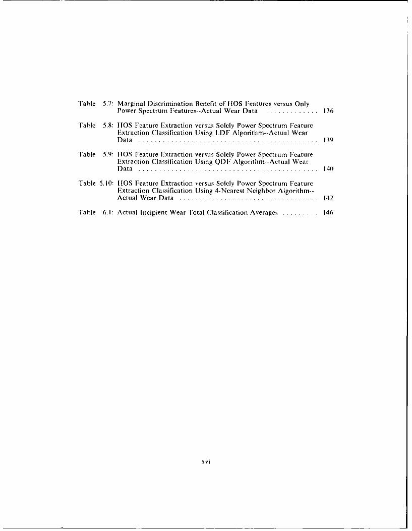
Table 5.7: Marginal Discrimination Benefit of IIOS Features versus OnlyPower Spectrum Features--Actual Wear Data ............. 136

Table 5.8: IOS Feature Extraction versus Solely Power Spectrum FeatureExtraction Classification Using LI)F Algorithm--Actual WearD a ta . . . . . . . . . . . . . . . . . . . . . . . . . . . . . . . . . . . . . . . . . . . . 139

Table 5.9: [HOS Feature Extraction versus Solely Power Spectrum FeatureExtraction Classification Using QDF Algorithm--Actual WearD a ta . . . . . . . . . . . . . . . . . . . . . . . . . . . . . . . . . . . . . . . . . . . . I 1(0

Table 5.10: IIOS Feature Extraction versus Solely Power Spectrum FeatureExtraction Classification Using 4-Nearest Neighbor Algorithm--Actual Wear Data .................................... 142

Table 6.1: Actual Incipient Wear Total Classification Averages ......... 146

xvi

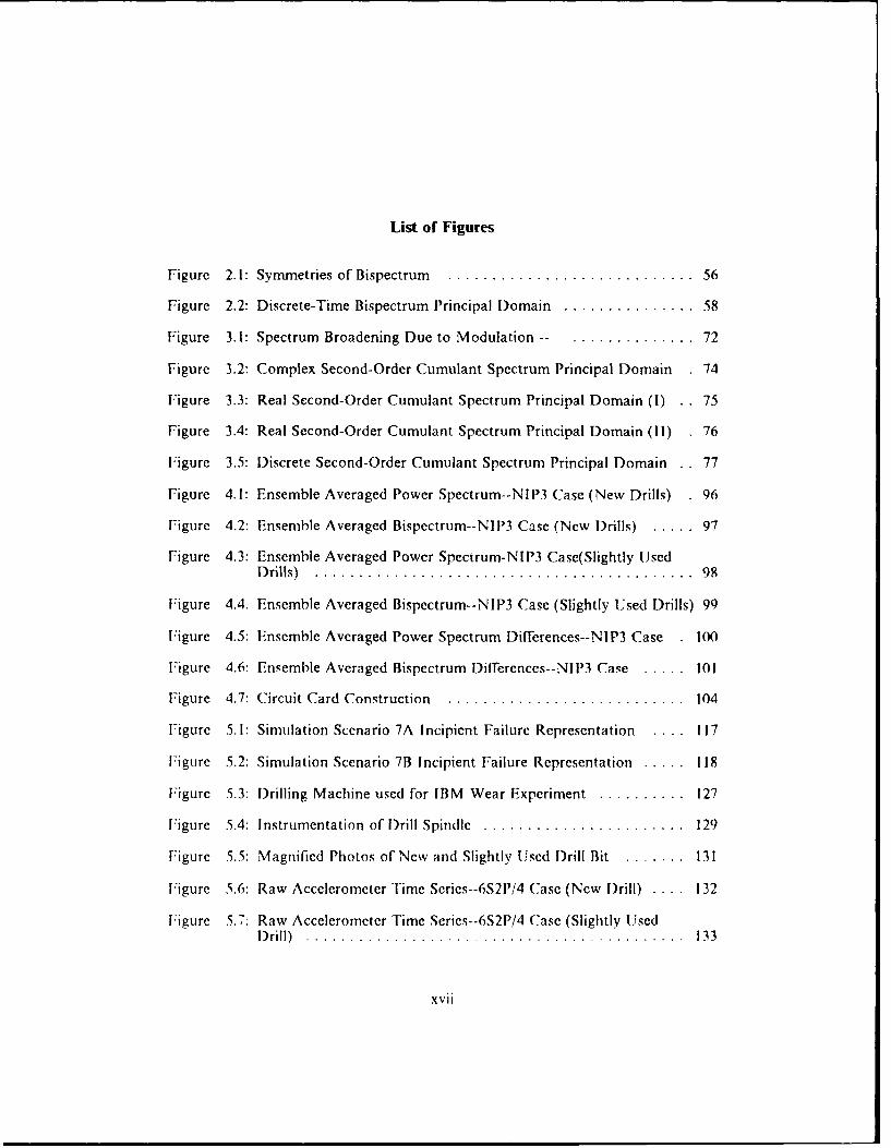
List of Figures

Figure 2. 1: Symmetries of Bispectrum ............................ 56

Figure 2.2: Discrete-Time Bispectrum Principal Domain ............... 58

Figure 3.1: Spectrum Broadening Due to Modulation --. ............ 72

Figure 3.2: Complex Second-Order Cumulant Spectrum Principal Domain 74

Figure 3.3: Real Second-Order Cumulant Spectrum Principal Domain (I) . 75

Figure 3.4: Real Second-Order Cumulant Spectrum Principal Domain (11) 76

Figure 3.5: Discrete Second-Order Cumulant Spectrum Principal Domain . 77

Figure 4.1: Ensemble Averaged Power Spectrum--NIP3 Case (New Drills) 96

Figure 4.2: Ensemble Averaged Bispectrum--NIP3 Case (New Drills) ..... 97

Figure 4.3: Ensemble Averaged Power Spectrum-NIP3 Case(Slightly UsedD rills) . . . . . . . . . . . . . . . . . . . . . . . . . . . . . . . . . . . . . . . . . . . 98

Figure 4.4. Ensemble Averaged Bispectrum--NIP3 Case (Slightly Used Drills) 99

Figure 4.5: Ensemble Averaged Power Spectrum Differences--NIP3 Case 100

Figure 4.6: Ensemble Averaged Bispectrum D3ifferences--NIP3 Case ..... 101

Figure 4.7: Circuit Card Construction ........................... 104

Figure 5.1: Simulation Scenario 7A Incipient Failure Representation .... 117

Figure 5.2: Simulation Scenario 7B Incipient Failure Representation ..... 118

Figure 5.3: Drilling Machine used for IBM Wear Experiment .......... 127

Figure 5.4: Instrumentation of Drill Spindle ....................... 129

Figure 5.5: Magnified Photos of New and Slightly Used Drill Bit ....... 131

Figure 5.6: Raw Accelerometer Time Series--6S2l1/4 Case (New Drill) .... 132

Figure 5.7: Raw Accelerometer Time Series--6S2P/4 Case (Slightly UsedD rill) ........................................... 13 3

xvii

Chapter I

Introduction

1.1 Introduction

This dissertation is concerned with the problem of detecting incipient faults

of rotating machinery. Because of their periodic nature, these types of physical

systems are mathematically represented as cyclostationary processes. Rotating ma-

chine research studies have proposed various monitoring methods (Micheletti, 1976,

and Jetly, 1984) but for reasons such as instrumentation difficulties in obtaining

measurements at or near the cutting surface of rotating tools, implementation of

most monitoring methods in industry is limited. Some of the better monitoring

techniques appear within the vibration analysis literature (Braun, 1986, and Shives

and Mertaugh, 1986) where vibration monitoring is shown to significantly reduce

the cost of maintenance, increase reliability, and decrease the probability of cat-

astrophic failure of rotating machinery. Milner (1988) lists bispectrum analysis, a

particular higher-order statistical (HOS) method, as a possible approach for moni-

toring vibration of small rotating machines in a NASA spacecraft. lowever, he

did not investigate bispectrum analysis due to the lack of adequate computational

methods. IGS methods arc defined in this study as statistical approaches which

analyze stochastic processes and their generated time series data associated with

nonlinear and also nonstationarY phenomena. The bispectrum provides a first

glimpse at nonlinear effects as it is the Fourier transform of the third-order moment

2

function of a stochastic process while the power spectrum, the Fourier transform

of the second-order moment, is most useful in problems estimating linear processes.

Recent findings (Dan and Mathew, 1990) conclude that no single condition moni-

toring method appears suitable for all machine operations and material combina-

tions. Consequently, condition monitoring research is better directed towards

improving instrumentation effectiveness, collecting better data on the functional

relationship between wear and measured parameters, and developing sensor fusion

methods which combine data from different sensors and features to improve system

monitoring accuracy.

There are many examples of models using a combination of sensors and

signal features for monitoring rotating tool wear. A vector autoregressive moving

average model developed by Yao (1990) used three axis tool force measurements to

estimate tool wear in turning of steel. Spindle vibration, cutting torque, and force

in monitoring of milling were input to power spectrum analyses to extract peak

values which were then input to a linear classifier (Elbestawi, 1989). A linear

classifier was also used for detecting crankshaft drill wear (Liu and Wiu, 1990) using

thrust force and axial acceleration amplitude signals. Acoustic emission spectrum

features and cutting force signals input to a neural network classifier demonstrated

the applicability of neural networks for noise suppression and also that there are

an optimal number of features (Rangwala and Dornfeld, 1990) for classification

purposes. Time and frequency domain characteristics of drilling forces for carbon

steel (Braun and l.enz, 1986) used a feature based on probability distribution mo-

ments of intensities and times of occurrences of a single oscillating signal pattern.

Braun and Lenz (1986) also stated that the choice of appropriate features, whether

single or combined, need to be based on test results or experimental databases.

3

These studies are a few examples of recent sensor fusion techniques in milling,

drilling of metals, and turning operations. Significantly with regard to this research,

feature construction of sensor signals in these recent studies is limited to the power

spectrum rather than any higher-order forms of spectra.

However, one study using bispectrum analysis as a tlOS technique to di-

agnose abnormal states of a machine from the normal one was conducted on gear

noise signal data (Sato et al., 1977). Its results showed that the gear noise signals

were almost periodical under proper loading and normal operating conditions. But

when heavy load conditions scored the gear surfaces, the periodic signal character-

istics were reduced and the signals appeared more random. This change in ran-

domness caused the modulus of the bicoherence Function, defined as the normalized

bispectrum with respect to power spectra, to decrease significantly. The more exact

diagnosis which considered the nonstationarv properties of the noises was left as

future work, and an experimental design strategy with an associated statistical

classification approach also was not evident in this first IIOS monitoring approach.

This first I lOS approach also investigated severe faults rather than incipient faults.

Incipient faults are those failures which are just beginning to appear in tile me-

chanical system.

To overcome the deficiencies of this first IIOS monitoring study this re-

search developed time series estimation procedures based on a nonstationarY or

crmulrant spectrum representation of the stochastic process under study. An exper-

imental design strategy and statistical pattern recognition framework was imple-

mrented to allow strong inferences from the data anaiyst. Furthermore, the

developed I lOS approach is evaluated for its abilitv to detect incipient, rather than

severe, faults. lhus, the types of monitoring problems addressed in this research

4

are more difficult than those previously studied. The developed IJOS approach

combines different forms of spectrum measurements (power, second-order

cumulant, and bispectrum) from sensors in a statistical classification scheme not

only to improve a monitoring system's classification performance, but also to reduce

its sensitivity to variables other than machine condition. These variables include.

but are not limited to, process environment parameters such as workpiece material

construction, cutting conditions, and noise. The developed IIOS approach is a new

type of sensor fusion technique which Dan and Mathew (1990) state as one of L~ie

most important open areas in condition monitoring research.

1.2 Problem Statement and Scope

The goal of this study was developmeni of a new analytical approach for

detecting incipient faults in physical systems which have a periodic driving force

mechanism generating potential signature data. The approach is the first to incor-

porate nonstationary (second-order cumulant spectrum) in addition to nonlinear

(bispectrum) and linear (power spectrum) characteristics of signature time series for

use as feature sets to improve the discriminatory power of a multivariate classifier.

Signature denotes signal patterns which characterize a specific system state.

Investigation of hispectrum analysis as a fault detection approach is moti-

vated by the fact that fault processes of rotating mechanical structures are known

to generate highly nonlinear time series data through the generation of sum and

difTer-nce frequencies (Braun, 1986). Nonlinearity is a result of intermodulation

between the frequency components of the driving process and produces spectra with

sideband structure. Without phase information, the presence of nonlinearities is not

5

detectable. The bispectrum captures this relative phase information among fre-

quency components. Investigation of cumulant spectrum analysis is motivated by

the fact that the signal data generated by faults in physical systems tinder study is

not only nonlinear, but also nonstationary due to the modulation effects of the

random fault mechanisms.

A good condition monitoring approach is insensitive to parameter changes,

noise disturbances, and nonlinearities which are intrinsic to the random processes

under study. So evaluation of the developed 110S approach includes marginal and

sensitivity studies of both simulated and actual experimental databases. Marginal

analyses determined the incremental value of I lOS features to power spectrum fea-

tures for discrimination and classification tasks. Sensitivity analyses determined the

impact of different classification algorithms, stochastic process parameters, and

noise on classification performance of classifiers utilizing spectral feature sets with,

and without, HOS information.

Simulation experiments of modulated signals explored potential robustness

properties of the new I IOS approach. Single tone amplitude and phase modulation

indices of a cosine-wave carrier signal (representing the periodic driving force of a

rotating machine system) and standard deviation of Gaussian noise are the simu-

lation parameters. Incipient faults such as initial wear of rotating machinery can

appear as amplitude and phase modulation changes. More emphasis is directed to

changes in phase modulation as amplitude modulation changes are assumed related

more directly to deviations in the process environment such as differences in

workpiece properties and cutting parameters rather than slight changes in process

state. Single tone modulation and the values chosen for the modulation index pa-

rameters should not limit the applicability of the simulation study results. In-

6

creasing the complexity of the signal modulation simulations would generate

additional frequency interactions and modulations and consequently provide more

frequency support in each of the higher-order spectral principal domain regions.

lence, the possibility of strengthening, rather than weakening, the value of the

1OS approach is afforded by increasing the complexity of the modulation simu-

lation experiments. Analyses of simulated data provide a first step in developing

estimates of actual classification error rates and also allow an evaluation of the im-

pact of Gaussian noise on classification using feature sets with and without 1 OS

information.

Since not much condition monitoring research addresses high-speed circuit

card drilling of epoxy-glass composite, IBM (Austin) conducted an experimental

drill wear study. Ramirez (1991) discusses the IBM circuit card manufacturing

process and drilling mechanics which generated the experimental drill wear data.

An indirect online wear monitoring approach using drill spindle acceleration, dis-

placement, and speed responses was investigated. A major conclusion of the

Ramirez (1991) study was particular vibration power spectrum harmonics from the

thrust axis accelerometer were the most useful responses for drill wear monitoring.

Also, since circuit card material composition plays a key role in generating vi-

bration, variations in card construction can mask the effects of wear of vibration

power spectra. The developed tIOS approach is investigated for its potential use

in the industrial environment by analyzing IBM experimental (trill wear data of

three factors: drill bit age, circuit card stack material, and chip load cutting condi-

tion. Accelerometer data obtained were from three axial positions (X,Y, and Z)

gathered on two types of bits defined by their number of circuit card holes drilled

(0 and 8000), two types of stack materials (NIP and 6S2P), and two types of chip

7

load (3 and 4 mil/rev). Chip load is the amount of axial distance travelled by the

drill bit tip in a single revolution or rotation. Actual wear data analyses will dem-

onstrate the marginal contribution of I lOS features to power spectrum features for

detecting incipient faults of manufacturing drill bits. Actual wear data analyses will

also add supportive evidence for further investigation and possible implementation

of the new i1OS approach in an industrial environment.

Both simulated and actual time series data represent incipient failure con-

ditions rather than new and definitely worn conditions of a rotating machine proc-

ess. Intuitively, it should be harder to detect slight or moderate wear than advanced

wear of rotating machinery. This is logical as signals used to characterize advanced

wear are usually more pronounced than those signals characterizing slight wear.

Wear condition of drill bits from the IRM experimental study were optically

checked under a microscope to accurately classify wear states. Because time series

waveforms are already grouped for their "similarity", cluster analyses are not

needed. Simulated and actual experimental data analyzed in this study are highly

non-Gaussian and nonlinear based on the I linich (1982) bispectrum statistical tests.

Hence, feature extraction rather than an optimality approach (Shumway, 1982) is

the technique used for time series discrimination and classification.

Both background noise and signal propagation media interfere with signa-

ture signals. Although there is some determinism due to the rotating machine's

periodic driving force mechanism, each of the signal types (noise, propagation, and

signature) is characterized hy an element of unpredictability. I lence, an ensemble

of signals for different states of cyclostationary processes are analyzed to ensure an

effective study of alternative classification approaches. Probability of false alarm

and probability of detection are the main performance measures. These measures

are averaged over the signal ensembles to decrease the variability of these per-

formance estimates.

1.3 General Research Approach and Presentation

This research focused on the development of two new methodologies:

cumulant spectrum estimation (second-order) and HOS feature extraction. In

Chapters 3 and 4, the new methodological developments are discussed which build

upon the background material given in Chapter 2. The HOS approach developed

in this work is tested with both simulated and actual physical phenomena to inves-

tigate and quantify the benefits of HOS estimation and feature extraction for in-

cipient fault detection. New estimation code to perform second-order and

third-order cumulant estimation of time series is developed. So besides the

bispectrum, the second-order cumulant spectrum is investigated and employed in

discrimination and classification tasks. Presentation of results to just the second-

order cumulant spectrum is due to time constraints and some technical problems.

Because a large number of measurements result from the spectral transformations

of the raw time series, a IIOS feature extraction algorithm is developed to combine

the most useful spectral measurements for incipient fault identification. Appropri-

ate measures of effect;vcness to evaluate the relative merit of spectral feature sets,

with and without IIOS information, are devised for both simulated and actual ex-

perimental studies. These measures of effectiveness are in the results section of

Chapter 5 after each experiment description.

Chapter 2

Background

2.1 Introduction

Detailed information on the major methodologies investigated to develop

a new analytical approach to the research problem is given in this chapter. First is

a description of existing incipient fault detection techniques for rotating machinery

using vibration signals. Second is an examination of the statistical theory and

models which permit interpretation of multivariate or group differences. Some

special considerations for use of multivariate approaches for time series discrimi-

nation and classification are discussed. Third, different types of stochastic processes

and the mathematical functions used to describe them are defined. Existing theory

related to higher-order statistics (HOS) concludes the chapter.

2.2 Existing Incipient Fault Detection Techniques

Although many types of signals are used for diagnostic monitoring of ro-

tating machinery, there are more examples of the demonstrated use and success of

vibration monitoring for significantly reducing the cost of maintenance, increasing

reliability, and decreasing the probability of catastrophic failure of rotating ma-

chinery (Braun, 1986, and Shives and Mertaugh, 1986). One success is TRACOR

Applied Science's (Austin) vibration monitoring program for the United States

9

10

Navy to improve the reliability and maintainability of the rotating machines on

their TRIDENT submarines and surface ships (Milner, 1990). They use signature

analysis of the accelerometer outputs, a common vibration monitoring technique.

Other incipient fault detection techniques using vibration signal monitoring include

demodulation of high frequency acceleration signals, statistical analysis of acceler-

ation amplitude, process modelling or parametric approaches such as auto-

regressive moving average (ARMA) time series ri odels, phase-locked processing,

cepstrum analysis, transient analysis, Htilbert transforms, and general pattern re-

cognition. These major techniques are summarized for a general understanding of

their strengths and weaknesses. Braun (1986) and Shives and Mertaugh (1986) have

complete discussions of these methods including schemes that combine some of

them.

Signature analysis of acceleration outputs is used in many commercial ap-

plications in addition to TRACOR's use for the Navy. Specific topics of analysis

bands, resolution, accelerometer type and its placement, instrumentation, and

presentation of accelerometer output are peculiar to the particular application.

However, a common thread among all applications is the reliance on association

of a particular failure mode with features of the vibration power spectrum. Tones

and other power spectral features present in rotating machinery vibration are gen-

erally due to predictable causes. There are many published relationships of faults

versus power spectral features for many different types of machines and their com-

ponents. Braun (1986) contains the theory and applications of many different

methods within the field known as mechanical signature analvsis. Signature analysis

is a very common technique as it has general applicability and proven success ror

a large variety of machine types. Also, the computation of the spectral amplitude

il

at selected frequencies and the association of amplitude increases with specific

faults is a necessary first step of several other techniques (general pattern recogni-

tion, trend analysis and .ocess modelling at key frequencies, transient and

cepstrum analysis).

High frequency demodulation of acceleration signals extracts relatively low

frequency information from a high frequency signal that has been amplitude mod-

ulated by a mechanical defect. It is mostly applied For bearing fault detection. At

the ,cry early stages of a bearing fault, impulses due to the rolling element passing

over the fault will be very short in duration, and can extend as high as 300 kllz (Bell

et al., 1985). The impulses excite resonant modes of the machine and the envelope

of the resulting time signai is the amplitude modulated component of the dej'ect

signal. The envelope signal will contain discrete peaks with periodicities deter-

mined by the input rate of the defect. After effectively bandpassing the signal,

power spectral analysis of the envelope will produce a harmonic series with a fun-

damental Ifequency that is olated to the bearing frequencies. Other general areas

of application of this technique include fault detection of gears and fluid film

hearings, and seal rub analysis (Darlow et al., 1975 and Drago, 1979). Because of

the high frequency range used vith ti, tec!.z,iquc, there is a high defeC. ignal-to-

noise ratio which is often stated as an advantage. However, an asroiatcd ltikad-

vantage is the requirement that the particular frequency within the high range must

he predetermined hefore filtering and demodulation is performed.

Weighted likelihood ratio processing and kurtosis are two statistical tech-

niques used to process amplitude signals. Weighted likelihood ratio processing is

described later in this chapter so only kurtosis processing is described here. A

"universal" behavior noticed in wear-induced failures is that localized defects ap-

12

pear first and distributed types of defects follow. Hence, induced vibrations often

have an impulsive character with the appearance of a localized defect, changing to

a more continuous function over time. The sharp peaks at the onset of defects af-

fect the tails of a probability density function (pdQ, and moments of the distribution

such as kurtosis can enhance the sensitivity to changes occurring at the pdf tail.

Kurtosis is the normalized fourth moment of a probability density function and

emphasizes the peakness of a particular signal pattern. Normalization is accom-

plished by removing the mean from the data and dividing by the fourth power of

the standard deviation. Kurtosis as a statistic is considered as an indication of

Gaussian versus non-Gaussian densities as it is equal to three for all Gaussian

densities. One example of the practical use of kurtosis is in the area of rolling ele-

ment bearing fault condition (Dyer and Stewart, 1979). The kurtosis value for good

bearings followed the Gaussian distribution value of three while significantly de-

graded bearings had large variations in the normalized acceleration distribution.

These large variations led to kurtosis values significantly different from three. The

authors stated more tests including simulation results for performance evaluation

are needed before conclusive remarks can be made on kurtosis as a fault indicator.

Process models are methods of detecting changes in expected waveform

structure. This technique generally involves mathematically modelling the system

outputs to determine if abnormalities exist in the signatures by statistically com-

paring them to normal model output. The extraction of features from the

parametric spectrum can mimic the methods applied to non-parametric spectra.

Another feature extraction approach is directly using system identified parameters

that describe the data (ic. AR, MA, ARMA). Classification of automobile engine

faults in a production assembly-line using a nearest neighbor classifier was based

13

on this latter type of feature extraction approach (Gersch, 1986). The Kullback-

Leibler measure of dissimilarity was employed which assumes the time series are

Gaussian-distributed (Kullback, 1959).

An approach related to Kalman filtering methods is based on analysis of

residuals after fitting of the parametric model to data. Variations in residual mag-

nitude, or statistical distributions different from normal meaning the fitted model

is no longer appropriate, can indicate a change in signal patterns. Specifically, an

approach called the Dynamic Data System (DDS) uses operational data from a

mechanical system and applies ARMA mathematical models to extract features

from the data with a high degree of sensitivity. The DDS model is combined with

statistical quality control chart concepts to monitor for abnormalities with a very

limited amount of data (Wu, 1977).

Phase-locked processing describes a general class of special processing

techniques that efficiently extract and filter periodic signals. Use of phase-locking

gives equivalent results in both time and frequency domains. This technique uses

encoders to give an integer number of pulses per revolution (Braun and Seth, 1979).

The number of pulses from the encoder should be equal to two to the power of the

number of pulses per revolution as the discrete Fourier transform (DFT) is usually

computed with a Radix 2 fast Fourier transform. The rotationally locked compo-

nents are located at multiple points in the I)FT indexed by p = N/M where N is

the number of pulses analyzed per revolution and M is the number of points in one

period. By employing a filter whose response is set to zero for all p 4# NIM the ex-

traction of the periodic signal from additional non-coherent interferences is

achieved. If additional signals non-coherent with the rotational frequency of the

14

machine exist, windowing is employed to minimize errors in the signal extraction

process due to possible leakage problems.

Cepstrum analysis is used in echo detection and deconvolution problems.

Braun (1986) has a detailed discussion of the use and problems in the computation

of cepstra. A common signal processing problem is the analysis of signals which

are composed of a wavelet and one or more echoes which may overlap. A simple

form of this composite signal is x(t) = s(t) + aos(t - t). Distortional effects such as

noise, overlapping of echoes and the wavelet, and different transmission paths ob-

scure the echo arrival time and basic wavelet shape. The signal plus echo may be

modelled as the convolution of s(t) with a time function 5(t) + a06(t - t) and the

separation of these two convolved signals is performed with operations in the power

cepstrum analysis. For example, if x(t) = s(t) x h(t), then

In I X(o,) 2 = In I S(o) I2 + In I 11(o)) 12. There is also complex cepstrum analysis

which is more general than the power cepstrum as inverse operations can recover

the original time signal. Both the power and complex cepstrum methods are im-

pacted by smoothness and bandwidth of the wavelet. Additive noise is another

major degrading influence in the effectiveness of cepstral methods. A wide band-

width and smooth wavelet spectrum is necessary for a less erratic wavelet cepstrum

which subsequently helps distinguish echo spikes from the wavelet cepstrum. A

majority of rotating machinery applications using cepstrum analysis are on gear

faults (Randall, 1982). Generally, it has been determined that gears in good con-

dition normally contain frequency sidebands of nearly constant amplitude over time

in the power spectrum. Changes in the number and amplitude of the sidebands are

proposed as indicative of a deterioration of a gear's condition and the cepstrum is

able to detect this change with an increase in amplitude of a single line. Thus, an

15

advantage of using a cepstrum approach is not being confounded by several sets

of periodicities in the power spectrum causing difficulty with a visual interpretation

of the data. However, Braun (1986) states this method is an interesting approach

to analysis of convolved signals, but it must be treated with caution and care for the

interpretation of its application to machinery diagnostic problems.

Because of their origins, transient signals usually have different durations,

peak amplitudes, repetition rates, frequencies, and bandwidths. Transient signal

detection schemes exploit varying degrees of a priori waveform structural informa-

tion. Most transient processors perform two primary functions: event capture and

transient analysis (Owsley and Quazi, 1970). Event capture involves continuous

loop data recording with a trigger signal that causes transfer to permanent data

storage. The trigger signal is driven by a simple detector of energy increases.

Transient analysis depends on the application and so varies significantly. Fourier

analysis is used to select key features such as the center frequency of a narrowband

transient and its bandwidth to classify the transient. Other extracted features in-

clude pulse duration and repetition rate (Nolte, 1968).

Ililbert transforms are another way to easily extract envelope information

from a modulated time signal. The H ilbert transform differs from the Fourier

transform because it leaves the signal in its original domain. It shifts the value of

a time signal by 1/4 wavelength or a 90' phase shift in frequency domain. Bell et

al. (1985) use the Ililbert transform for incipient fault detection of rolling element

bearings.

Many examples of machinery monitoring systems in the literature can be

categorized as a general pattern recognition approach. One excellent commercial

example is the statistically based system developed at Oak Ridge National Labora-

16

tory for continuous, on-line, unattended surveillance of dynamic reactor signals

(Smith, 1983). Their monitoring system is based on identification of changes in the

power spectrum of measured variables where change is detected by using

discriminant functions formulated to emphasize relevant features. Discriminants

were constructed to detect the following: (1) a fluctuation in the integral power of

the spectrum; (2) spectral shape changes; (3) deviations in the magnitude of indi-

vidual spectral estimates at a given frequency; and (4) shifts in the frequency of

spectral peaks. Their system, typical of most pattern recognition systems, used

classification functions based on Bayesian estimation decision theory preceded by

a heuristic feature extraction process to transform the raw time series data. What-

ever features are used, the determination of thresholds is usually determined by ex-

perience where monitoring systems are fine-tuned as more information on the

process is obtained. Features are used for classification purposes and their statis-

tical properties affect monitoring performance. However, few references or studies

describe monitoring systems based on formal statistical aspects because of the dif-

ficulty of acquiring information and databases from sufficiently large sample pop-

ulations (Paul, 1977). Statistical pattern recognition is the general framework of

this research and simulation and actual time series databases are from sufficiently

large sample populations. The statistical approach employed in this research is

unique for constructed features are not restricted to power spectrum estimates, but

also include estimates of two higher-order spectrum forms.

2.3 Measuring Differences Among Multivariate Populations

Since the developed monitoring approach is described and evaluated from

17

formal statistical aspects, this background section first discusses the types of anal-

ysis questions that arise when confronted with the problem of measuring differences

among multivariate populations. Decision theory definitions introduce the theore-

tical basis underlying discrimination and classification tasks. Estimation of class-

conditional probability density functions (pdfs) or discriminant functions under

various levels of assumption are discussed and compared. Performance assessment

issues of the developed feature extraction sets input to multivariate classifiers using

design and test sets are discussed. Mathematical details that address the partition-

ing of the total sample variance, a fundamental step in the development of tech-

niques which separate multivariate populations and statistical considerations in

measuring population differences, conclude the background section.

Several analysis questions are postulated when investigating multivariate

group differences. First, are the groups significantly different with respect to their

multivariate descriptions? This is a multivariate equivalent to the sample

(univariate) t-test on population means. A sample mean vector, or centroid, for

each population is formed, and the null hypothesis of equal population centroids

is tested using I lotelling's T' statistic, or equivalently, Wilks' A statistic when con-

sidering only two groups. If' more than two groups or populations are involved,

multivariate analysis of variance looks for differences among population centroids.

Second, what role do the measurement variables play in separating the groups? A

discriminant function which can be a linear, quadratic or some other transformation

of the measured variables answers this question. Its evaluation objective is to yield

similar values for cases from the same population and different values for cases

from difTerent populations. Examining the discriminant function plovides insight

on which measurement or feature variables are most important in separating the

18

groups. The population separation problem using only information about one of

the variables at a time usually is not very efficient and is suboptimal. For example,

two individual variables may not be good discriminators by themselves, but when

combined they may be highly effective. Developing a discriminant function corre-

sponds to the search for a vantage point which provides a view with maximum

group or population separation. This underlies the motivation for performing ItOS

estimation and feature extraction in addition to traditional power spectrum meth-

ods. It is conjectured that higher-order forms of spectra combined with power

spectra will provide a better vantage point. Moreover, 1OS features will just sim-

ply be better discriminators than power spectrum features. Discriminant functions

can be constructed using stepwise selection of variables similar to stepwise selection

of variables used in multiple regression. When there are more than two groups.

multiple discriminant functions can be developed (beyond this study's scope).

Third, if responses or measurements of the variables are known for a new observa-

tion, to which group does the case belong? This is the multivariate classification

problem while the first two questions concerned multivariate discrimination. In

many applications of discriminant analysis, classification is the major objective.

For example, if there is a description of new drill bits and slightly used drill bits in

terms of spectral features calculated at times of different wear states, these spectral

features can then be used in classification rules which would specify whether an-

other drill bit is a member of one of the wear categories. Thus, classification rules

are developed from the discriminant functions.

Consider definitions from decision theory to explain the basis underlying

discrimination and classification. A decision rule partitions a space into regions

U,, i- 1, .... ,N where N is the number of classes. An object, or time series. is

19

classified as coming from class (o, if its corresponding vector representation, x lies

in region Q. The vector representation x can either represent direct time series

measureiaents or features, , (xi), which are functions of the x,. The boundaries

between regions are called decision surfaces. Assume that prior probabilities,

P (w ,) are known that an object comes from class a), (i = 1, ... , N). Information in

the form of a vector, x, is then determined for an object to be classified. The Bayes

minimum error rule is formed by comparing the posterior probabilities of belonging

to each class using the information vector and classify according to whichever is

larger:

P(o'klX)>P(il x) for allj * k -*Xeik.

Since the posterior probabilities are rarely known, they need to be estimated from

samples of known classification. Another formulation of the Bayes minimum error

rule is obtained through application of Bayes Theorem to determine the class

membership probabilities:

P X) p (x I w,)P (w1)P (ml ) = p Wx

which results with

p (x I "k) P ((,)k) > p (x I ij) P (o)), for allj 6 k -+ x C . [I]

If p (x I a,. the class-conditional pdfs are known, the problem is solved by substi-

tution of x into [I] for the time series being classified and finding the largest value

ofp (x I w,) P (w,). But similar to P (o), I x), the p (x I (a,) are probably unknown and

require estimation rom a set of classified samples.

20

Bayes minimum error rule for the two case situation is:

p X1())> --((02)

P(XlC2 ) < P(CO 1)

This rule minimizes the overall error assuming equal misclassification costs but for

industrial manufacturing situations where misclassifying a worn tool may be more

seious than misclassifying a new tool, a different criterion which considers the dif-

ferent misclassification costs (Bayes minimum risk) may be more appropriate. Ad-

ditionally, if the prior probabilities of a new time series are unknown, a minimax

rule designed to minimize the maximum possible risk is used. Iland (1981) develops

all three rules expressed as functions of x using the class-conditional pdfs p (x I Q),).

Considering the absolute values of the probabilities not as relevant as their relative

magnitudes allows more general rules. For the two-class situation the general rule

is:

/()>constant *+ X E {where h is called a discriminant function. As before, the discriminant function will

require estimation from classified samples. Estimation procedures are categorized

by the level of assumptions used for the likelihood function: parametric and non-

parametric. Non-parametric approaches estimate the class-conditional pdfs or the

discriminant functions without any knowledge about their parametric form. In

parametric approaches, assumptions are made about the form of the class-

conditional pdfs or (liscriminant functions and estimation of the unknown func-

tional parameters are performed with the classified samples. Parametric and

21

non-parametric estimation methods applied in this research study are discussed

next.

2.3.1 Estimation Methods

If the class-conditional pdfs or discriminant functions forms are known,

then the tasks of discrimination and classification are simplified as likelihood func-

tion ratios with various risk thresholds are compared for its solution. Unfortu-

nately, this knowledge rarely exists but the general parametric form may be known

from some theoretical knowledge or from a study of the sampling distributions. In

this situation, samples are used to give estimates of parameters of the class-

conditional pdfs or more generally, sample distributions are used to estimate the

parameters of the discriminant functions. However, when simplifying assumptions

are not defendable, non-parametric methods are also applied. Lachenbruch (1975)

and Hand (1981) outline and compare various parametric and non-parametric pdf

estimation methods. After preliminary experimentation and application of several

of these estimation methods, three were chosen for their consistent classification

performance of the experimental data described in Chapter 5. The k-nearest-

neighbor (k-NN) method was the non-parametric method applied to actual time

scries data. Two parametric approaches, linear and quadratic discriminant func-

tions, were also applicd to the actual data. Linear discriminant functions were

constructed for the simulated experiments.

Assuming a multivariate normal distribution for the spectral features of

each time series class resulted in discriminant rules based on the pooled covariance

matrix (yielding a linear function) or the individual within-group covariance matri-

22

ces (yielding a quadratic function). Feature measurements are placed in the class

from which it has the smallest generalized squared distance or the largest posterior

probability.

The squared distance from feature vector x to class to is

d,(x) = (x - iZ.)'V,'(x - R.)

with V. being the pooled or within-class covariance matrix and K_, being the feature

variable means in class a. The class specific density at x from class 0) is:

f/(x) = (2 1r-P12 I V, I ' 2exp( -. 5d,2 (x))

and posterior probability of x belonging to class co is computed by applying Bayes

Theorem:

AW I X) PJ.(x)p(to Ix) - -P~fk(x)

ZPfx)

where the summation is over all the classes.

Now, the generalized square distance from x to class co is

D , 2(x) = d 2(x) + g1(()) + g2(t)

with gl(ro) = log. I V, I if within-class covariances are used (quadratic function),

g,(o) = 0 if pooled covariance matrix is used (linear function), g2(o) = - 2 log.(q,)

if prior probabilities are unequal, and g2(o) = 0 if prior probabilities are equal.

The posterior probability of x belonging to class a) is then

23

(exp(-.5D'(x))

Thus, an observation, or feature variable set, is classified into class a if setting a)

equal to Q produces the largest posterior probability or smallest value of D.f(x).

The difference between the generalized squared distances of the class means is the

squared Mahalanobis distance measure.

Non-parametric estimates of class-specific probability densities of feature

sets are computed with a k-nearest neighbor approach. Squared Mahalanobis dis-

tance calculated from the pooled covariance matrices is used to determine proxim-

ity. The k-nearest neighbor does not have a complicated approach to its selection

of the smoothing parameter, k, as it is based on which gives the best classification

performance. Following Hand (1981), consider the probability that a point will fall

in a local neighborhood L of x for the multivariate pdf p (x I o)) as

0 = JP(yI )dy.

The following approximation is made if 1. is small and has volume V:

0 - 1 (IO,) • V

which vields

p (xI ) V.

24

A pdf estimator for 0 is then comput2d by the proportion of the n. ;ample points

falling in the local neighborhood L Assign k to denote the number of sample

points ,alling in and obtain 0 = k/n.. which then leads to the estimator defined

as:

A (x ) - k

The volume V is made dependent on the data by fixing k and determining V needed

to enclose the k nearest points to x. Next, combine all the classes' sample points

into one set of n points such that En. = n. The hypersphere of volume V which

just encloses k points from this combined set is found. Now consider that among

the k points, k., occur from class co.. Thus, a k-NN estimator for class cm, is de-

fined:

Ax ,, k,(Xl)GP) n .V "

kThere are also the estimators P (o,,) - and ~(x) = ;. Application ofn nV

Bayes Theorem givcs:

A (Xl,,)P(Ii) _ ( = =k(x) k k

nV

So, the following classification rule is generated: classify x as belonging to class i if

k, = max.(k,).

25

2.3.1.1 Advantages and Disadvantages of Applied Estimation Methods

A disadvantage of k-nearest neighbor is distance: e-om the feature vector

to all of the sample points must be determined. hlence, all of the sample points

must be retained and this can increase the amount of computer time for classifica-

tion. flowcver, there are branch and hound techniques to reduce the amount of

data required so quicker computation is possible (lland, 1981). It also has the

theoretical disadvantage of not being a pdf (lland, 1981). Assuming parametric

forms for the class-conditional pdfs allows quicker classifications of new samples

and no large databases of trairing set points are necessary to retain. However, an

incorrect distributional assumption will incur an associated cost in terms of an in-

creased misclassification error rate, but tis cost may be acceptable if computa-

tional advantages outweigh it.

2.3.2 Other Estimation Approaches Considered

Several other estimation approaches investigated during the study were

weighted likelihood ratio and logistic discrimination. These methods were not used

to generate final study results for thcir results were not as good as the others.

I lowever, weighted likelihood ratio processing is described here as it was applied to

data proposed as a fiture application for the developed IIOS approach. l.ogistic

discrimination is described because of its sirnilarit- to the linear discriminant ap-

proach.

Milner (1088) found that a likelihood ratio weighting technique of vibratic,11

power spectra to be superior in detection performance for a wide range of problems

26

in pump and fan data. This approach assumes a Gaussian density function of the

logarithmic amplitude of the power spctrum. The binary test hypotheses, (a)

power spectrum indicates new object (K,), or (b) power spectrum indicates slightly

used object (K), alter this Gaussian density in mean level only, and the power es-

timates of each bin or frequency are assumed independent. Given the definition of

the natural logarithm of the likelihood ratio derived from the Bayes criterion for

binary hypotheses, the log likelihood ratio is:

in!t =I J ( - S, - ,noi)' ( S, - Mid )2_2

i= I i

where S, is amplitude of the object vibration power spectrum in decibels (dB) at

frequency i, in,, is average log amplitude of frequency i of new object vibration

power spectrum, nt, is average log amplitude of frequency i of slightly used object

vibration power spectrum, and M is the number of useful freqiiency tones. Com-

pleting the square and canceling common terms [2] becomes:

M

In ( . ) = S i (M I - Mod [3](71

If [3] is greater than zero. the object is classified as slightly used. If [3] is less than

or equal to zero, then the object is classified as new. Implementation of this test

27

first computes power spectra for the set of new objects and for the set of slightly

used objects. Then values for m, and rmi, are computed, and the bins with the

largest mean shift as compared to their stability receive the largcst weights. These

weights are consequently indicators of the relative importance of specific frequen-

cies as indicators of object wear. A weighted sum over all usefl frequency infor-

mation for the particular time series is computed to detect the worn .k .dition.

Weaknesses of this approach outweighed any advantage of incorporating

global spectral characteristics. The weaknesses are assuming the class distributions

are different in mean level only, and that power estimates at each frequency are

independent so a diagonal covariance matrix can be used. These assumptions were

not appropriate for the actual experimental data analyzed in this study.

Logistic discrimination is a partial distribution classification method as it

assumes the log-likelihood ratio is linear in the measured parameter vectors:

In L(x IK,) } l,+flX 4in L( ) = fio' +/'x, [4]

where fl' = (fil, , fir). Anderson and Richardson (1979) show three advantages

for using logistic discrimination versus a fully distributional or distribution-free

classification approach. First, the model given at [4] gives a simple form for the

posterior probabilities:

flo' + In C + fl'x(I ± exp(fl0' + In C+ fi'x))

28

where C = [I/I12, and [1, is the proportion of sample from K. with (s= 1,2). Sec-

ond, once the parameters (fl0',/f and C) are estimated, the allocation of a new ob-

servation or feature vector set requires only a linear function calculation:

flo' ± C + fl'x.

Third, this same estimation procedure is applicable with either continuous or dis-

crete predictor variables.

2.3.3 Mathematical Development of Analysis of Variance

A fundamental step in the development of statistical techniques based on

separation of multivariate populations is the partitioning of the total sample vari-

ance into components representing within class variation (variance of individual

observations about their class's centroid), and among class variation (variance of

individual observations around the centroid for the combined sample). This parti-

tioning process is the multivariate equivalent of the partitioning sum-of-squares

accomplished in the univariate analysis of variance (ANOVA) model. In univariate

problems, hypotheses concerning equality of means can be tested using the two

sample t-test when two groups are involved, or F-tests using statistics derived from

one-way ANOVA when multiple groups are considered. In multivariate analysis,

equality of mean vectors or centroids across groups or populations are tested. For

the two population case, I lotelling's T' provides the multivariate equivalent to the

two sample t-test and test statistics derived from one-way multivariate analysis of

variance (MANOVA) provide the appropriate hypothesis tests for the multiple

population situation. When there are only two groups or classes as in this research

29

study, the one-way MANOVA is equivalent to the two-sample Ilotelling's V test

and this is the presented approach.

2.3.3.1 Partitioning of Variance

Consider developed expressions representing the partitioning of an arbi-

trary linear combination of measurement variables into within and among class

components. Notation is defined:

x,,* i = 1,2, ... , nk; j = 1, 2, , g represents the observed value on the j*

variable from the ill case in the kth class. There are g groups or classes and p

measured variables. Class k includes n, observations.

A= [xiAk ... xik]' is a p-element colun vector representing the complete

multivariate observation for the ill sample in the kik class.

= E.i, ... l,]' is a p-element column vector representing the centroid

of the k" class.

The elements of jk are the sample means for each variable computed for

observations in the k'h class, and denoted ; j = 1, 2,..., p.

= ( nk)n ,_k is a p-element column vector representing the combined

class centroid.

The elements of i are the sample means of each variable computed forg

observations from all g classes, and n is the total sample size: n = 5 n,.

Consider a special vector representation of the matrix of sums-of-squares

and crossproducts of deviations from the mean. This matrix, when divided by (n-I)

for n total observations, is the sample covariance matrix. Also consider the fol-

30

lowing product of the vector of deviations from the combined class centroid for a

specific observation and its transpose:

XIk -

Xl2k - 3F2

(-ik -X)(_ik - X= [(xilk - -V),(X 2 k - 2) .... (xiPk -Tr)]

Xipk - Yp

[(Xilk _ 1)2 (Xhlk - .i1)(X2k - 2) .. (Xi1k -7)(i -

(Xi2k - . 2)2 ... (X12k .V2)(Xlpk -. r) . [5]

(xipk - y.)2

The matrix which results from this multiplication of a column times a row vector

is a p x p matrix of squares and crossproducts of the deviations of the observation

for each variable from the corresponding sample mean. If these vector products

are calculated for each observation in the kMh class and the results are summed, the

following square matrix will result:

Y'kS(xlk - )( ik - 2_ )'

(Xik -- ) "

......... ( il )(Xlpk 6]

(X12k- 2 )

2

Z-xpk - !

31

Summing [6] across g classes results in another symmetric matrix which looks like

[6] except for the double summations which accumulate results for all observations

across the g classes has the sums-of-squared deviations of each variable from its

mean on the diagonal. The off-diagonal elements are sums of crossproducts of de-

viations from the mean for all pairs of variables. If this matrix is scalar multiplied

by 1/(n - 1), the sample covariance matrix for the combined class (total covariance

matrix) is obtained. The summation of [6] across all classes is the total sums-of-

squares and crossproducts, and is denoted by T:

g nk

E ( -, u! Gr" - [7]k=lI =lI

The total covariance matrix is:

g

S - Tandn -- n [8(n-I)k=1

A similar computation, performed by substituting the centroid for the k",

class for the overall centroid and summing only over the observation subscript (i),

yields the within class sums-of-squares and crossproducts matrix denoted by IV, for

the kA class:

nk

[Vk -- / k - 9k)(_Xk -!-k).

32

If Wk is scalar multiplied by I/(nk - 1), the sample covariance matrix for the k"h class

is obtained.

For the discriminant analysis problem, the T matrix is partitioned into

matrices attributable to the within class (W) and among class (A) differences. This

partitioning process is analogous to the partitioning of the total sum-of-squares in

the univariate ANOVA model except this is working with vector rather than scalar

quantities. If the W matrix is multiplied by l/(nk - 1) = l/(n - g), the result is a

pooled estimate of the covariance matrix or within class covariance matrix

(multivariate analogy of the pooled estimate of variance used in univariate two-

sample t-test and the pooled estimate of the error variance used in univariate

ANOVA). This matrix is denoted by S. where S - I W.n-g

There are different ways to manipulate combinations of time series meas-

urement or feature deviations from their centroids in the development of

discriminant functions and statistical tests for centroid differences. In a discussion

res,-icte, to only linear discriminant functions, g, computational advantages will

result from a g that is linear in the components of the observation measurements

x, or features which are functions of the x, Considering only manipulating linear

combinations of feature vector deviations from their centroids, scores like the fol-

lowing are calculated:

p

fk = ajxo - - UM1

where a, is a coefficicnt, i represents an observation index or i'" time series, and j is

a feature variable index. In matrix terms. [10] is:

33

a,

a 2

fk = 9'(xk- ) where [II]

The partitioning of the total sum-of-squares of thef, scores into within and

among class components is required for developing the discriminant function. Since

9 nk gn

k=11=1 k=1i=l

= a'Ta [12]

and recalling the partitioning of the T matrix:

a'Ta = a'Z |ka + a'Aa = a'Wa 4 a'Aa. [13]

[13] is an equation with scalar terms as pre and post multiplication of the p x p

matrices by q' and a results in I x I matrix products. Pre and post multiplication

by a results with the first term of [13] representing the sum-of-square values of the

linear function defined by the coefficients in a evaluated for deviations of each fea-

ture vector observation from its class mean. The final term of [13] is a weighted

sum-of-squared values of the linear function evaluated for deviations of class

centroids from the combined class centroid. Thus, [13] is used to partition the total

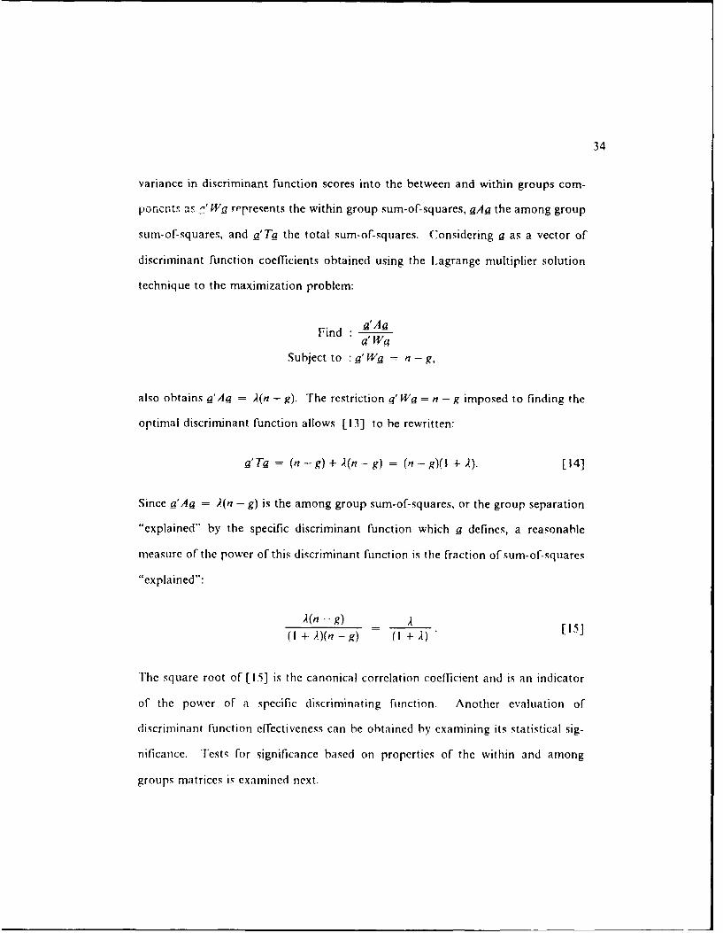
34

variance in discriminant function scores into the between and within groups com-

poncnts as -W -a represents the within group sum-of-squares, aAa the among group

sum-of-squares, and a'Ta the total sum-of-squares. Considering a as a vector of

discriminant function coefficients obtained using the Lagrange multiplier solution

technique to the maximization problem:

a'AaFind . 'A

a' Wa

Subject to : a'Wa = n- g,

also obtains g'Aa = ,(n - g). The restriction g' Wg = n - g imposed to finding the

optimal discriminant function allows [1 3] to be rewritten:

0-Ta = (n-g)+ ,(n-g) = (n-g)(l + ). [14]

Since a'Aa = ,(n - g) is the among group sum-of-squares, or the group separation

"explained" by the specific discriminant function which a defines, a reasonable

measure of the power of this discriminant function is the fraction of sum-of-squares

"explained":

A(n - g) A 1

(+ A)(n -g) (I1) [1A]

The square root of [15] is the canonical correlation coefficient and is an indicator

of the power of a specific discriminating function. Another evaluation of

discriminant function effectiveness can be obtained by examining its statistical sig-

nificance. Tests for significance based on properties of the within and among

groups matrices is examined next.

35

2.3.3.2 One-Way ANOVA and MANOVA

Consider the univariate one-way ANOVA model:

Xlk J A+-ak--r. + k i I .... , nk; k -- I,... ,g [16]

where x,, is the observed value of an interval scaled criterion variable, 'U is the

overall mean, ct is an effect due to the presence of the 0rA treatment or experimental

condition, and f, is an error term analogous to the r, term in the multiple regression

model. In this model, i indexes a specific observation in one of the g groups of

observations collected using the various experimental conditions. By letting

pk= + ot±,, where pk represents the k1, group mean, [16] is

Xik =-Ilk +- ik" [17]

If the random errors are independent normally distributed with common variance,

statistical tests for the significance of the ,,s are performed. The hypothesis tested

is:

11 : Al = 2 Pg

I1 : at least two ik, s differ.

The significance of the differences among group means is interpreted by

partitioning the total sum-of-squares ofx,, deviations from their sample mean into

the within groups component which represents an estimate of error variance, and

the among groups component which measures deviations from the null hypothesis

of no group differences. Let .?k represent the sample mean for the k"' group, and

the overall sample mean. The partitioning is then:

36

g nkg nk

/jXk - X) L Z JL(Xlk - -k) + (k - -V)]

k=ii=i k=1 =1

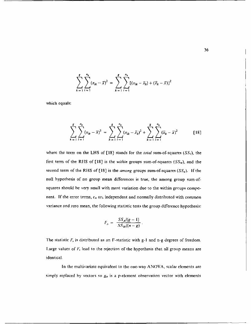
which equals:

g nk g nk g nk

(X ~ Z _Zj) XIk _ ik)2±+ X (Vk_ )2 [18]k-I 1=1 k=l l=1 k=l 1=I

where the term on the LHS of [18] stands for the total sum-of-squares (SSr), the

first term of the RIIS of [18] is the within groups sum-of-squares (SS"), and the

second term of the RttS of [18] is the among groups sum-of-squares (SSA). If the

null hypothesis of no group mean differences is true, the among group sum-of-

squares should be very small with most variation due to the within greups compo-

nent. If the error terms, Flk ar. independent and normally distributed with common

variance and zero mean, the following statistic tests the group difference hypothesis:

SSA/(g - 1)SSw/(n - g)

The statistic F, is distributed as an F-statistic with g- I and n-g degrees of freedom.

Large values of F lead to the rejection of the hypothesis that all group means are

identical.

In the multivariate equivalent to the one-way ANOVA, scalar elements are

simply replaced by vectors so S,k is a p-element observation vector with elements

37

x,k, 1A is a p-element centroid for the overall population centroid, o is the effect of

the k", treatment, and Elk is an error vector. Hence, the tested hypothesis is:

Ho1 :- .....

I11 : at least two _is differ.

Rejecting the null hypothesis leads to the conclusion that there is a difference

among some of the group centroids.

Similar to the univariate case, the significance of the difference among

centroids is investigated by partitioning the sum-of-squared deviations of the ob-

servation vectors, x, , from the combined sample group centroid denoted by _. This

is the same problem where the partitioning process results in expressing the total

sum-of-squares and crossproducts matrix, T, as the sum of within and among

groups components, W and A, or T = IV + A. If the null hypothesis is true, matrix

W will be similar to matrix T. The evaluation of the relative magnitude of within

and among groups sum-of-squares is complicated by the fact that they are p x p

matrices. I lowever, Wilks (1963) developed a test based on the determinants of the

W and T matrices. lis procedure represents a likelihood ratio test of the hypoth-

esis that all groups have identical centroids and the Wilks' lambda statistic, A, is:

jIl _ (WIIA+ WI 171

Thus, it is seen that small values of A lead to rejection of the null hypothesis of no

group centroid differences. The sampling distribution of A is complex because the

number of groups (g), observations (n). and variables (p), are all parameters, but

38

various approximations for evaluating A are available. One is the F-statistic for the

one-way MANOVA model developed by Rao (Tatsuoka, 1071):

F Ails IS A ls-p(g - 1)/2 + )

A I/S""' 'p(g - I)

where p is the number of variables, g is the number of groups or treatments,

i n - I - (p 4 g)12 and

S = p2(g_ i)2 2 4_±(g 4) 2

where s= I if the numerator and denominator equals 7ero. The statistic F, is dis-

tributed as F,1 .,2 where v, = p(g- I) and v2 ms- p(g - 1)/2 4- 1. The critical

region for the test is:

Reject !!, : p =. k

if F,> . where a is the significance level for the test, and v, and '2 are the nu-

merator and denominator degrees of freedom, respectively.

2.3.4 Classifier Performance Measurement Criteria

A critical aspect for comparing alternative feature extraction approaches

input to several classification algorithms is a fair and consistent estimation of their

total misclassific-tion erro- rates. Lachenbruch (1975) discusses the leaving-one-

out, or jacknife, method for computing error rate estimates. This method estimates

the discriminant rule oritting one sample time series and then r'Fylies that rule to

classify the remainir, observational time series. Misclassifications are tallied afler

39

the jacknife process is iteratively done for all observations. The various types of

error rates are discussed in the next section. Another measure of classifier per-

formance is the total cost of misclassification. Stated 'rom a decision thcory per-

spective, a Type I error, or lower probability of detection, is worse than a Type 11

error, or higher probability of false alarm. An actual total classification cost can

be computed for alternative classification approaches if the respective misclassi-

fication costs are known.

The easiest way of estimating a classifier's misclassification rate is calcu-

lating iow many of the design or training set observations are misclassified. Early

work in pattern recognition research implemented this approach but it was discov-

ered that the estimated error rates underestimated the actual error rate of the

classifier. This is because the classifier or decision rule is optimized on the design

set and unless this set perfcctly represents the population distribution, a new set.

which is random sample drawn from the same distribution, will be different and so

the classifier will not be optimal. The error rate calculated by reclassifying the de-

sign set is called the apparent error rate. This is distinguishale from the actual error

rate which is the expected error rate of tv c'-nstructed classifier on future samples

from the same population distribu tion as the training set.

The siriple approach of reclassifying the design set has an optimistic bias

so researchers investigated methods for estimating the actual error rate from a de-

sign set (Ilills. 1966). llowevcr, problems with still optimistically biasing the esti-

mation of actual error rate caused researchers to concentrate on estimating the

expected actual errnr rate. One way to estimate the expected actual rate, the

leaving-one-out method, gives an unbiased estimate and works well with non-

(;aussian observations (Lachenbruch 1975). This is the method for computing

40

classification error rate estimates for the experimental data in this research. But

another research strategy was not to restrict feature performance comparisons by

constructing a classifier and estimating its error rate from only a design set of data.

In simulation experiments, other independent time series were generated and used

as test sets so application of a designed classifier to these new sets yielded a

straightforward estimate of the actual error rates for the various feature

extraction/classification approaches. Special considerations are now discussed

about discrimination and classification of data that are in time series form.

2.4 Discrimination and Classification of Time Series

There are two major approaches for viewing, analyzing, and interpreting

time series--one based on the time domain and another based on the frequency or

spectral domain. The theoretical development of time series methodology has ex-

hibited a leader-follower pattern, first emphasizing one domain, then the other.

Spectral (Fourier) analysis decomposes functions representing fluctuating phenom-

ena in space or time into sinusoidal components that have varying frequencies,

amplitudes, and phases. Several texts specify the necessary mathematical condi-

tions for the existence of the Fourier transform (Brigham, 1974 and Bracewell,

1978). Ilere, let it suffice that the Fourier transform does exist for waveforms

physically observed in nature (Bracewell, 1978). For a given random process,

x = {x(t), t e RJ, the continuous Fourier transform (CFT) definition X(f), is:

41

X (f) = FX(t)e- i 'rftdt,

and the inverse Fourier transform definition x (t) is:

x (t )= F.X()er"df.

The inverse Fourier transform shows how the x random time function can be de-

scribed by a superposition of complex sinusoids e" r , with the amplitude and phase

of those sinusoids lying in the spectral band between fandf+ df defined by

X(f)df. Hence, X(f) is a complex amplitude spectral density function. For ex-

ample, if x has the dimensions of volts, then X (f) has the dimensions of volts/lIz.

In addition to the Fourier transform being a function that represents the amplitude

and phase at each frequency, it is an effective tool mathematically, statistically, and

computationally. It is of great mathematical use because the convolution operation

occurs so often and is greatly simplified by the Fourier transform. Statistically, the

large sample properties of the Fourier transform are much simpler than those of the

corresponding time domain quantities. Computationally, fast Fourier algorithms

allow evaluation of interested parameters more rapidly with smaller round-off error

than by direct time domain evaluation. Spectral analysis has an inherent consist-

ency and efficiency in its application because the power spectrum and all higher-

order spectrum density functions use the estimates provided by the direct discrete

42

Fourier transform (DFT) of the raw time series. For these reasons, spectral analysis

is the time series processing method implemented for feature development and

subsequent input to a classifier. The decision for employing a feature extraction

approach rather than an optimality approach is discussed next.

Consider the time series discrimination problem where the observation of

a discrete parameter time series x at each of T points in time is given and the

standard objective is to classify the observed time series into one of k mutually ex-

clusive and exhaustive classes with an overall low misclassification error rate. The

univariate sample time series can be represented as x = (x(0) ... x(T- 1)) and so

the classification problem concerns finite dimensional random vectors where

standard multivariate approaches are applied. However, Neyman-Pearson likeli-

hood or Bayes criterion rules are usually applied to classifying multivariate vectors

where T is small, and the learning population is adequate for estimating the un-

known parameters. Generally, this is not the case for time series data. For exam-

ple, the simulated time series analyzed in this study have T of approximately 1200,

and the learning populations contain a maximum of 250 time series. Furthermore,

the actual time series data analyzed in this study have T of approximately 2500, and

the learning populations contain a maximum of 60 time series. Thus, the compu-

tations for discriminant function calculation and performance evaluation will in-

volve inversion of large covariance matrices which are also not of full rank. I lence,

the numerical difficulties of time domain calculations motivated investigation of

other approaches for time series discrimination.

Shumway (1982) gives two distinct alternative approaches of spectral time

series discrimination. The first, or optimality approach, assumes very specific

Gaussian models and solutions are developed to satisfy definitive minimum error

43

criteria. This approach generally requires prior knowledge of the time series or

signal waveforms so that either linear or quadratic discriminant functions can be

constructed. Shumway discusses the use of the frequency domain discriminant

analysis approach where matrix inverses can be replaced by simple sums involving

discrete Fourier transforms (I)FT) and spectral density functions. Since the DFT

of a weakly stationary process produces nearly uncorrelated random variables and

variances approximately equal to the power spectrum, estimation and hypothesis

testing problems are formulated in terms of sample spectral densities with simple

approximate distributions. Shumway (1982) gives results which make discriminant

analysis in the frequency domain framework a very promising approach. But

Shumway noted the danger or limitation of the optimal approach (either time or

frequency domain) is the fact that inappropriate assumptions of time series distrib-

ution structure can cause an "optimum" solution to be only a rough approximation

to the actual problem. In fact, the time series measurements within the exper-

imental databases in this research were found to be highly non-Gaussian and non-

linear based on the Ilinich bispectrum-based statistical tests (Ilinich, 1982). Thus,

feature extraction, the other distinct approach to time series discrimination and

classification, was the approach followed in this study. A IIOS feature extraction

algorithm developed to combine various types of spectral features of the simulated

and actual time series is discussed in Chapter 4. Time series are most often real-

izations from a stochastic process and mathematical representations called

covariance functions used to characterize its behavior are defined next.

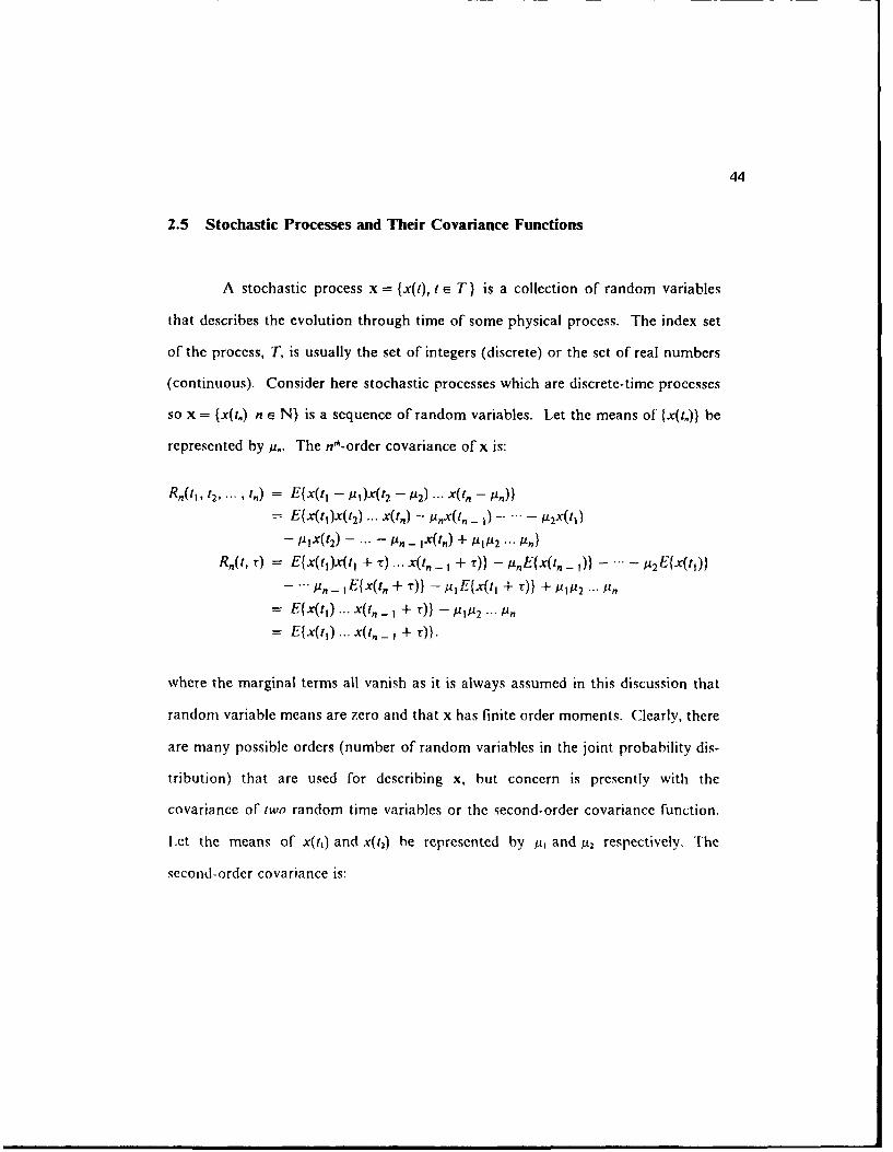
44

2.5 Stochastic Processes and Their Covariance Functions

A stochastic process x = {x(t), t e T} is a collection of random variables

that describes the evolution through time of some physical process. The index set

of the process, T, is usually the set of integers (discrete) or the set of real numbers

(continuous). Consider here stochastic processes which are discrete-time processes

so x = {x(t,) n e N) is a sequence of random variables. Let the means of {x(t,)} be

represented by u,. The n"-order covariance of x is:

Rn(tl, t2, , t) = E{x(t, - p1)x(t 2 - P2) ... x(tI -/t)

- E(x(tI)x(t 2 ) .x.t,) - PnX(t, - 1) - - 2x(t)

- PIx(t2) - -"- - An - 140tn + JUI02 ... An}

Rn(t, r) = E{x(tI)x(t 1 + T) ... x(t, _ ± r)} - 1)} ....- 2 E{x(t,))

- p-IE{x(t + T)} - pE{x(I + r)} +P J12 ... Pn

= E{x(t) ... x(t,- I + r)) -/P tA2 ... P,

= E{x(t) ... x(t,, - I + T)).

where the marginal terms all vanish as it is always assumed in this discussion that

random variable means are zero and that x has finite order moments. Clearly, there

are many possible orders (number of random variables in the joint probability dis-

tribution) that are used for describing x, but concern is presently with the

covariance of two random time variables or the second-order covariance function.

let the means of x(ti) and x(t,) be represented by p, and p2 respectively. The

second-order covariance is:

45

R.(tl, t2) = E{x(t, - M)x(t 2 - A2))

= Efx(tl)x( 2 ) - A 2x(t - tAIx(t 2) + £91'2}

R.(t, r) = E{x(t1)x(t1 + r)} - P 2 E{x(ti)} - p1E{x(t 4 r)} + 9 19 2 [19]= E{x(t)x(t1 + r)} - 1#2

= E{x(t1)x(t 1 + T)}.

where the second term vanishes as random variable means are zero. The second-

order covariance is thus a bivariate expected value which provides a summary of the

degree which two random time variables are associated.

When [19] is a function of only the time difference or lag parameter, T,

with T = t,- t,, so that

R.x(tl, t2) = R.x(T),

the x process is known as a wide-sense or weakly stationary stochastic process.

Requiring all marginal and joint density functions of a random process to be time

independent, or strictly stationary, is frequently too restrictive an assumption in

practice as it is hard to find a strictly stationary random process. But there are

physical situations in which the process does not change appreciably during the

time it is being observed, H fence, wide sense or weak stationarity is adequate to

guarantee that the covariance of any pair of random variables are constants inde-

pendent of the choice of time origin. In these cases, the relaxed wide sense sta-

tionary assumption leads to a convenient mathematical model to closely

approximate reality. Ilowever, it is the mathematical convenience when assuming

weak stationarity which tends to prevent the proper investigation and applicability

of other forms of joint random variable distributions of a particular stochastic

process under study. Even if nonlinearity of a stochastic process is addressed

46

through HOS analysis, these studies also frequently assume stationarity of the ran-

dom process.

For stationary time series, there exists a uniquely defined decomposition

into a deterministic and a purely nondeterministic component which are mutually

orthogonal (Wold, 1954). This decomposition forms the basis of a time-domain

analysis of a given stochastic process generalizing the well known properties of

stationary processes. Also, spectral analysis, rather than the time domain, provides

the powerful methods of harmonic analysis (Wiener and Masani, 1957). Harmonic

analysis is possible for stationary processes because spectral representations in the

form of Fourier-Stieltjes integrals exist for the process variable and the associated

covariance functions:

x(t, = e f dAx(f)

where A,(.f) is a stochastic process with orthogonal increments. Cramer (1960)

considers certain classes of nonstationary processes having similar spectral repres-

entations. lie shows that without requiring A,(f) to have orthogonal increments,

one is led to a class of stochastic processes called harmonizable or rvclosiationarp

processes.

A process is strictly cyclostationary if:

E{x(tl) ... x(t,)} = E{x(t I + k1) ... x, + k7)

47

for k e N, for all n, and Tdenotes the period. When [19] is periodic in t with period

1" for a fixed time difference or lag parameter, r, the second-order covariance is:

Rxx(t 1, t2) = E{x(t,)x(t 2)}

= E{x(1 + T)x(t, + T± r)},

and the x process is known as a weakly cyclostationary stochastic process.

Cyclostationary processes are processes whose joint distributions vary over time,

and are thus nonstationary, but whose parameters vary according to periodic

functiuns. Cyclostationary processes are a class of stochastic processes which ap-

pear in the physical world via a mechanism that provides some deterministic struc-

ture in the observed time series. These processes are therefore appropriate modcls

for phenomena involving cycles or when there exists some underlying periodicity to

the data-generating mechanism.

To successfully deal with problems of statistical inference connected with

stochastic processes, it is crucial to have an appropriate and convenient type of

analytical representation for the particular class of processes under study. This

analytical representation should express in mathematical form the essential features

of the random mechanism assumed to generate the process. This ensures accurate

assessments are made on the various statistical questions arising from process gen-

eration. Consequently, I IOS in addition to power spectrum, representations were

used and developed in this research so that the intermodulation and nonlinear effects

of random fault mechanisms of cyclostationary processes such as rotating machine

systems are captured in the physical process representations. Background infor-

mation on existing IIOS theory is given next.

48

2.6 Higher-Order Statistical (HOS) Theory

For single time series, the idea of polyspectra, or higher-order Fnectra, was

originated by Blanc-Lapierre (1953). Algebraic and analytic detail was provided by

Leonov and Shiryaev (1959) and Shiryaev (1960), who also considered the spectral

representation for a cumulant, rather than for a product moment. Shiryaev attri-

buted this idea to Kolmogorov. Brillinger (1965) generalizes the definitions of these

earlier papers by considering k-dimensional time series. Brillinger (1965) also de-

veloped a theorem which explained the importance of cumulants rather than prod-

uct moments. The actual term, polyspectrum, is due to Tukey who began the

development of a calculus relating polynomial operations to higher-order spectra.

The power spectrum is a complex-valued function of frequency and is de-

Fined as the Fourier transform of the second-order stationary covariance function,

= E [X(t)X(t + T)]:

P f " 2(TC12,rf dT.P (f ) = c2 fr)o T d.

Now, a specific case of polyspectra is the third-order spectrum, or bispectrum, a

complex-valued function of two frequencies and defined as the double Fourier

transform of the third-order stationary covariance function,

c,(r, r2) +[X(t)X(t ± r,)X(t + r)]:

B(A ,f 2 ) = r(r,, 7 2)e 2n (f,r, + f2T2) drI dr2.-- 00 - ,t

49

From examining each spectrum's Parseval relations:

E[y(t)] l P(f)df, and

(27)2 J J0 B(A fA ) df, df2,

it is clear that the power spectrum represents the contribution to the second mo-

ment over a particular range of frequency, and the bispectrum represents the con-

tribution to the third moment over of a particular pair of frequencies. Nikias and

Raghuveer (1987) list a wide range of bispectrum applications. Specific examples

of nonlinear structure detected in a variety of time series using bispectral analysis

include: nonlinear interaction of ocean waves in shallow water (Ilasselman et al.,

1963), analysis of acoustic gear noise (Sato et al., 1977), and nonlinear energy

transfers in plasma (Kim and Powers, 1978). More sophisticated statistical appli-

cations of the bispectrum are within studies of nonlinear spectral transfer of energy

in turbulence (Lii et al., 1976, Van Atta, 1979, and Ilelland et al., 1979). Pro-

ceedings from the 1989 Workshop on Iligher Order Spectral Analysis (Nikias and

Mendel, 1989) contain some recent developments of bispectrum theories and ap-

plications of processing signals to extract information based on cumulants. The

latest developments of 1OS theory and its various applications are in the IEEE

Proceedings from the 1991 International Signal Processing Workshop on Higher

Order Statistics (Gcorgel, 1991). In this research, in addition to the hispectrum, the

second-order cumulant spectrum not constrained hy stationarity, is investigated for

50

providing feature information to a multivariate classifier to detect incipient failures

of rotating machinery.

2.6.1 Moments and Cumulants

Following Rosenblatt (1983), consider the random variables (X, ... , X,).

Let 4(t, ... , t,) be the joint characteristic function of the random variables

.(t.. tk) = E exp i X = CO. [20]

lfinixed moments EX' = E(Xv' ... Xv) =MI A

k k

v = ( Vk), vJ>0, IvI = Z vi V!= fvji!

exist up to a certain order I v I < k, they are the coefficients in the Taylor expansion

of 4' about zero

J'{=(it) X + o(1kd Ut ( )(,Ilk). [21]Id' <k IvIl <k

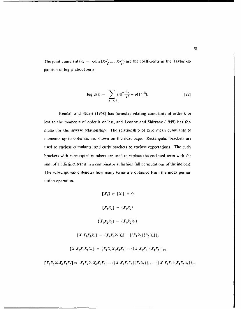
51

The joint cumulants c, = cum (Xv', ... , Xv:) are the coefficients in the Taylor ex-

pansion of log 46 about zero

log () = ( ) + o(1tI k). [22]

IvI -. k

Kendall and Stuart (1958) has formulas relating cumulants of order k or

less to the moments of order k or less, and Leonov and Shiryaev (1959) has for-

mulas for the inverse relationship. The relationship of zero mean cumulants to

moments up to order six art, shown on the next page. Rectangular brackets are

used to enclose cumulants, and curly brackets to enclose expectations. The curly

brackets with subscripted numbers are used to replace the enclosed term with the

sum of all distinct terms in a combinatorial fashion (all permutations of the indices).

The subscript value denotes how many terms are obtained from the index permu-

tation operation.

[X1] = {X1} = 0

[X, X2] = {XIx 2}

[XX 2X3] = {xIX 2X3 )}

[XIX 2X3X4] = {XX 2X.3.1X} - {{XX 2}{x 3X} X 3

[XIX 2X3 X4 XSJ = {XJX 2X3X 4X) - {{XIX 2X3 ({X4 X5}1}1

[X1X2XIX 4X5X'6] = fXIX 2X1X'4X5X(6} - ffI23V)56)5- {{X 1X2X3}{X 4 YXX 10

52

+ I(x1x 2}x 3x4}xX5X)1 15

These relationships show that cumulants are expectations with lower order

statistical dependence removed. If the cumulant of n random variables is desired,

the expectation of the product of all n random variables is constructed, and addi-

tional terms are added so the net result will completely vanish if any subset of the

variables is independent of any other subset. For the simple case of n = 2,

[X1X 2] = (X1X2) - (x,)Ix2), [23]

the RI IS of [23] vanishes if XA and X2 are independent. For n = 3,

[X X2 K3] (X1 X2X1 [24- (X,}{X4(X3) - [' 1X 2](X 3} - [X, X3]X 2} - [X 2 ]{1x}.

In the zero mean case, the last four terms of the RHS of [24] are zero, and so the

third-order cumulant and third-order moment are the same. If X, and XY2 and X., are

independent, the entire RIS of [24] is zero.

Rosenblatt (1983) showed that the existence of all moments up to order k

is equivalent to the existence of all cumulants up to order k. Nevertheless, the

bispectrum is defined as the Fourier transform of the cumulant sequence rather than

the moment sequence. Brillinger (1965) gives three reasons for this definition.

First, cumulants have better independence propertic. than moments as they are

constructed so each order cumulant has the dependence on lower order cumulants

removed. Second, for ergodic stationary stochastic processes, Fourier transforms

of cumulants are mathematically better behaved than Fourier transforms of mo-

ments. The third justification for te use of cumulants is if the process is stationary

53

Gailssian, then all of its kt-order moments for k > 3 do not provide any additional

information about the process. However, the cumulant function does provide ad-

ditional information as for k > 3, cumulants are zero for Gaussian processes.

Hence, the cumulant, rather than the moment, is the function needed to detect de-

partures from a Gaussian structure or linearity.

2.6.2 Mathematical Properties of The Bispectrum

Mathematical properties of the bispectrum are discussed in many JIOS lit-

erature references but Hinich and Patterson (1989) emphasize the concepts of hne-

arity, Gaussianity, and stationarity. Consider a time series, x(t) generated by the

linear inodel:

00

x(t) = a(n)e(t - n) [25]

where {r(t)} is a purely random series. The weighting function, or impulse response,

a(n). is real for physically realizable systems, and from causality, is zero for negative

n. If the series {f(t)} is Gaussian, then the original process {x(t)} is also Gaussian,

and has a zero bispectrium. But if the series {r(t)} is pure noise and non-Gaussian,

then {x(i)} is non-Gaussian, ano has a nonzero bispectrum. Also, [25] can be

nonlinear if {r(t)), the input proccss, and a(n) are dependent and {x(i)} will be

nonlinear even if {r(t)) is Gaussian, and the bispectrum will be nonzero.

Let {x(t)} be a itionary time series with zero mean, and assume that all

expected values and urns used exist. The power spectrum of [25] is the Fourier

transform of the autocovariance function C,_(t) = F [x(t + n)x(t)].

54

00

S (f) = C.(t) exp { -i2rfn}.n 0

If S (f) is constant, then {x(t)} is serially uncorrelated on a white noise process.,

The bispectrum of [25] is defined as the two-dimensional Fourier transform of the

bicovariance function C,,,(n,m) = E [ x(t + n) x(t + m) x(t)] which does not depend

on t because the process is stationary:

B (f 'f2)= eZC (nm) cxp ( -i27fln - i2nf2m).

The two frequency notation hides the three frequency interaction which is impor-

tant in bispectral estimation applications so three frequency notation

B (f, g, -f- g ) and the Cramer representation of[25] was introduced by Brillinger

and Rosenblatt (196 7 a):

x(t) J exp [i27rfn] dAx(f) [26]

where ( d1 ,(f)} is a complex stochastic orthogonal increments process, and the

integral defined in [26] is in Stieltjcs sense. Now, because [25] is real, dA,( -f) is

Whiteness of a series does not imply the series is purely random. This is important assome time series techniques do stop fitting a model when the residual errors appear to bewhite noise. The assumption of Gaussian residuals is made for the sake of convenienceas zero correlation (foes imply independence in the Gaussian case, but if the series is non-Gaussian, this assumption can lead to wrong inferences.

55

the complex conjugate of dA.(f). The spectral density at f of [25] is

S (f)df = E { dA,(f) dA,( -f)}, and the bispectral density for h = -f- g is

B (f, g, h) dfdg = E { dA,(f) dA.(g) dAb(h)}. [27]

Because of stationarity, [27] is invariant to time translations so for B (f, g. h) dfdg

to equal B (fg) dfdg for all f and g, the sum f+ g + h must be zero.

When {x(t)} is linear, [27] is shown by Brillinger (1975) to be

B (f, g, h) dfdg = A3A(f)A(g)A(h) [28]

where A (f) is the transfer function of the impulse response a(t), P3 = E {e(t)}, and

(c(t)} is the innovation process. The spectrum of the linear process [25] is

(f) = ,'A (f)A ( -f) [29]

where a, is the innovation process variance.

The right hand side of [28] is invariant to permutations of the frequency

indices f, g, and h = -f-- g. Thus, the bispectrum's symmetry lines are as shown

in Figure 2.1 on page 56. Symmetry means that if values of the bispectrum are

known at all points in one region about a symmetry relation, values in the other

region can be determined through either a permutation and/or conjugation opera-

tion.

56

IgO

Figure 2.1: Symmetries of Bispectrum

Because dA,( -f) = dA*(f), B) ( -f, - g, - h) dfdg = B' (f, g, h) dfdg. This skew

symmetry gives another three symmetry lines:

g = -f, h = -f(g = 0), and h = - g (f= 0).

[hus, the cone,

C = {fg: 0_ f,O g_<f},

is the principal domain region of the continuous-time bispectrum in the (fig) plane.

Principal domain is the minimum region or frequency space which estimates are

computed.

In physical reality, a continuous-time process is always sampled for some

finite period, so investig,ted processes are band limited at some cutoff frequency

57

f. Contribution of frequencies above the cutoff frequency to the process variance

is therefore zero, and so the continuous-time bispectrum is cut off at f = ±f,

g = ±f, and f+ g = ±f. Thus, the continuous-time set of positive support for

absolute value of [28] is the right isosceles triangle

IT = {fg : 0 <f:fc, O < g<f:f+ g = f,}

shown at Figure 2.2 on page 58. But there is also a discrete-time bispectrum where

Hinich (1989) shows the discrete-time bispectral density with r as the sampling in-

terval:

B, (fg,h) dfdg = E { dA(f) dA(g) d Ax(h)}

= ZIS B(f+--,g+ .h+---)dfdgk m n

(k + m+ n)forf+ g + h - r = 0, with signed integers k,m,n restricted to keep the

indices in the bispectrum's principal domain (Brillinger and Rosenblatt, 1967a). But

since there is band limitation atf, the summation is restricted to k,m, and n such

that

k m0 <f+--T -:9 0

and

_ (k±') + m f)

Sampling actually causes an infinite number of parallel symmetry lines defined by

2f~g = -!2- and f+ 2g - The cone C in Figure 2.1 on page 56 is ctt byf~g =..

58

both of these symmetry relations, but for a particular nx, the line f+ 2g = n is

at least to the line 2f + g = 2L. when both lines are within C. I lence, the principal

domain of the the discrete-time bispectrum, B, is the triangle

{fg: 0<f<1 , o gf, 2f~g

which is a proper subset of C. This triangle is the union of the sets IT and OT in

Figure 2.2. Statistical tests for Gaussianity and linearity (Hinich, 1982) and alias-

ing (Hinich and Wolinsky, 1988) of time series data use estimates calculated over

this discrete-time bispectrum principal domain region.

A/

IT

114t 1121

Figure 2.2: Discrete-Time Bispectrum Principal Domain

59

2.6.3 Bispectrum-Based Statistical Tests

Ashley et al. (1986) showed the Ilinich bispectrum-based statistical tests

(Ilinich, 1982) to have substantial detection power for many common forms of

nonlinear serial dependence (bilinear, nonlinear and threshold autoregrcssivc, non-

linear moving average). Also demonstrated was that the bispectral linearity test can

be applied to raw source data as well as to the fitting errors of an estimated linear

model. Consider now the development of these statistical tests.

If the mechanism generating a time series has non-zero terms in the third-

order cumulant function, then the bispectrum will be nonzero and vary with fre-

quency. This fact is the basis for the linearity and Gaussianity statistical tests

developed by Subba Rao and Gabr (1980) and Ilinich (1982). Even though Rao

and Gabr first implemented Brillinger's (1965) method for measuring the departure

of a process from linearity and Gaussianity by using bispectrum estimates of the

observed time series, their tests do not use the asymptotic properties of the

bispectrum developed by Rosenblatt and Van Ness (1965), Shaman (1965), and

Brillinger and Rosenblatt (1967a,b). There are two approaches to smoothing sam-

ple bispectra to obtain consistent and asymptotic Gaussian estimators with known

sampling properties for large samples. Rao and Gabr (1980) use a lag window

kernal to multiply the sample third-order covariance, or bicovariance, array com-

puted from a sample of the time series: this weighted covariance is then Fourier

transformed to yield a bispectral estimator. Ilinich (1982) applies a fast Fourier

transform to the data array, computes triple products of the discrete complex

Fourier coefficients, and then uses a two dimensional smoothing filter in the

60

bifrequency domain to obtain a bispectral estimator with known sampling proper-

ties. This allows for the tradeoff between variance and bias of the estimator. The

Ilinich FFT approach uses fewer arithmetic steps than Gabr and Rao's lagged

covariance products approach. Another element ;f Ilinich's faster computational

approach is the breaking of the data record into intervals and then averaging the

sample bispectra for the record blocks. Additionally, Rao and Gabr (1980) did not

develop test statistics for the significance of individual bispectral estimates. On the

other hand, the Ifinich statistical tests give chi-squared statistics for testing the

significance of the bispectra. For these reasons, the ltinich bispectral-based statis-

tical tests to detect departures from nonlinearity and non-Gaussianity are applied

to time series data in this research.

With a finite impulse response and two-frequency index notation, [25] is

Bx (ff 2I) = 3 A (f,)A (f2 ) A' (f +f 2 ), [29]

where p, = F. r:(t), A(f) = a(t) exp( -i2nrfn), and A* is the complex conjugaten-

of A. From [25] and [29] a functional relationship called the squared-skewness

function of {x(t)} is defined and is the basis of the I linich linearity and Gaussianity

tests:

I1(flf 2I 2 _"_ (ff) [30]

S (f,) S (f ) S (fA +.f2 ) ,'

I lence, [30] is a standardized third-order cumulant spectral function as it is the

square of the bispectrum normalized by the power spectrum product of each cor-

responding frequency. The degree of dependence between two frequencies is

measured by [3',]. If [25] is linear then [30] is constant over all frequency pairs

61

(ftf2) in the bispectrum principal domain. The test for Gaussianity of the time

series {x(t)} involves testing that [30] is zero. Since i = 0 for the Gaussian case,

a non-zero value of the bispectrum rejects Gaussianity. Brockett et al. (1987) has

a more complete discussion of these tests and Ilinich (1982) has the precise formu-

las and proofs concerning the test for linearity and the derivation of an

asymptotically normal test statistic based on [30].

2.6.4 Cyclostationary Processes and Higher-Order Spectra

IIOS research studies show that nonlinear phenomena can be studied by

computing higher-order spectrum estimates. Nonstationary phenomena can also

be studied by computing higher-order spectrum estimates which are not constrained

by the assumptions of stationarity. For example, there may be situations where it

is bencficial to compute estimates of the second-order cumulant spectrum and the

third-order cumulant spectrum rather than the power spectrum and the bispectrum,

respectively. This I IOS study conducted a time series estimation approach which

computed linear (power spectrum), nonstationary (second-order cumulant spec-

trum), and nonlinear (bispectrum) estimatzs of cyclostationary processes for con-

struction of feature information. Of interest in this research is mechanical vibration

monitoring and diagnosis for rotating machinery. In this situation, the periodicity

arises from rotation, revolution, or reciprocatior of mechanical structures such as

shafts, gears, pistons, or propellers. This work presents evidence that frequency

support in the second-order cumulant spectrum principal domain (2-CSPI)) region

provides additional and significant feature information to bispectrum and power

spectrum features for wear signal characterization of rotating machinery. Devel-

62

opment of the principal domain regions for the second and third-order random

variable cases is contained in the next chapter.

2.7 Summary

Pertinent details of the major methodologies investigated to develop a new

approach to the research problem were given ;n this chapter. Reviews of existing

incipient fault detection techniques show an approach which employs IlOS con-

cepts needs investigation. Measuring differences in multivariate populations, and

particularly time series, from a statistical perspective was discussed. Feature ex-

traction is the time series discrimination method employed as the Gaussianity as-

sumption for an optimality approach does not apply to the highly non-Gaussian

and nonlinear time series data analyzed in this research. Even though different as-

sumptions are made about the form of the class-conditional probability density

functions (pdfs) used to characterize population differences, explanations in a

Bayesian decision theory framework show that the class-conditional pdf is estimated

in a way so similar values result when the function is evaluated for features from

the same class, and widely differing values result when evaluated from different

classes. Statistical tests of the null hypothesis that the centroids of different classes

are equal are used. These tests are based on the partitioning of the matrix of

squared deviations of observational feature sets from the sample centroid into ma-

trices representing within and among class components. Closely related to dis-

crimination is classification which applies the decision rule to assign a multivariate

feature set with unknown class membership to its proper class. This research ap-

plied linear, quadratic, and 4-nearest-neighbor classifiers. An unknown time series

63

observation generated by a cyclostationary process, defined by "optimum"

discriminant feature sets, will be assigned to the class which has the highest classi-

fication function, or posterior probability value. Applying classification rules to

simulated and actual experimental time series data of known categories will result

in measures of the classification power of the rules and their respective extracted

feature sets. Major concepts of existing IlOS theory emphasize the importance of

justifying the use of certain limiting assumptions such as linearity, Gaussianity, and

stationaritv of the stochastic process under study. Use of proper spectral esti-

mation procedures which include cumulant spectrum estimation are investigated to

provide improvement to extracted feature information for cyclostationary time se-

ries discrimination and classification. The development of this new analytical ap-

proach is contained in the next two chapters.

Chapter 3

Cumulant Spectrum Estimation

3.1 Introduction

This chapter discusses the approach to cumulant spectrum estimation of

periodic time series data generated by physical systems such as rotating machinery.

Cyclostationary models are used to represent these physical systems as they contain

both deterministic and random components. The deterministic component is due

primarily to the constant periodic force of the machine. The random component

is due to various sources such as the randomness of the process under study (ie. the

process of wear), different operating and maintenance conditions (process environ-

ment), and randomness of the machine manufacturing process (no two machines

are exactly the same).

In the time domain, various orders of covariance functions can be used to

describe random processes. Alternatively, random processes can be characterized

by the Fourier transforms of these various covariance functions. This chapter pre-

sents the key ideas underlying second-order cumulant spectrum c.;timation for a

single time series. Second-order cumuldnt spectrum estimation is a new procedure

that provides information beyond the bispectrum and power spectrum estimation

of the experimental time series data described in Chapter 5. The spectral estimation

approach describes the estimation of stationary, cyclostationary, and nonstationary

processes in an integrated manner. It has the potential with further development

64

65

for use as tests for stationarity and periodicity of the observed time series but the

primary interest in this research is the use of second-order cumulant spectrum esti-

mates for feature extraction and incipient fault characterization of cyclostationary

processes.

This work is different from the previous HOS monitoring study (Sato,

1977) and other treatments of cyclostationary processes (Gladyshev, 1961 and

Ogura, 1971 and Hurd, 1969, 1989a, 1989b, and Gardner, 1989) in that it incorpo-

rates estimation concepts of several classes of stochastic processes (nonstationary,

stationary, and cyclostationary) in terms of spectral correlation functions calculated

over a second-order cumulant spectrum principal domain (2-CSPD) region. The

2-CSPD is derived from symmetry properties of the Fourier transform. There are

several important properties of the 2-CSPD region. First, the support of the

2-dimensional cumulant spectral measure for purely stationary processes is con-

strained to a diagonal line defined by f = -f2 in the fourth quadrant of the

2-CSPD space. Cramer (1960) and Brillinger (1965) state this property so this idea

is not new. Second, the support for strongly harmonizable periodically correlated

processes (Gardner and Franks, 1975 and lurd, 1989a, 1989b) or purely

cyclostationary processes (PCS) is constrained to a set of equally spaced parallel

lines to this stationary support set where the Euclidean line separation distance

between correlated spectral components indicates the period or cycle exhibited in

the data set. However, the new result demonstrated in this research is that calcu-

lated second-order cumulant spectrum estimates not on a purely periodic support

grid are those of concern and increased interest when studying incipient wear of

rotating machinery. The estimated frequency support not restricted to the funda-

mental periodic -omponents and their harmonics for both stationary and

66

cyclostationary support sets in the 2-CSPD represent intermodulations of the

stochastic process. These modulated frequency components are p;oposed to pro-

vide additional and better feature information for incy.J'nt wear signal character-

ization than periodic spectrum components.

3.2 Cumulant Spectra and Their Estimation

Let x (t,) ..- , x (t,) be N observations from a random time series sampled

on M = {n: n = 0,1, - 1,2, -2, ... . The {x (t,), n e M} are random variables and

this notation is equivalent to X(1), ... , X(N) with N jointly distributed random var-

iables with a common marginal distribution and zero mean, but lower case x is used

in time series literature. Consider the vector of time points

t = (1, ... tN) r. MN

where Mv = M x M x M x ... M . Let cur (t/N) denote the Nth-order cumulant

of the time series sample of any N dimensional subset {x(ti), x(t) ... , x(t,)} of the

jointly distributed random variables. In this notation.

cum(t/ I) = E [X(t)] = E [.x(t)] = 0 for each ! because common marginal distrib-

utions have zerc mean. Strictly stationary processes have cure (t/N) depending

only on the N-I time points denoted by the vector d = (12 - t ... IN, - t). Strictly

periodically correlated or cyclostationary processes have cun (t/N) depending only

on the N/T time points where T denotes the period or cycle and dcnoted by the

vector P = (,I, IIT).

67

Consider the general nonstationary case and transform a vector of time

points, t to its spectral representation, f=( f).The Nth-order curnulant

spectrum is now defined:

Cum S .(D N =ZI cum ( tIN )exp[ -i2( t'f)] [31]

A strictly stationary process has the Nth-order cumulant spectrum replaced by the

N-lIth order polyspectrum definition:

S, (fIN- 1) = cum (dIN) exp[ -i27r(d'fN. 1)]. [32]

dEM I-I

A strictly periodically correlated process has the the Nth-order cumulant spectrum

replaced by the Nth-order periodically correlated spectrum:

Applying [32] to [311, the general relationship between cumiulant spectra

andl polyspectra can he expressed as:

Cum S, ( f/N) = 5 (f', + -- fN) S, (fIN - 1, [34]

where (5(f) is the Dirac dlelta fuinction. The RIIS of [341 iq zero for

f - fi + ... #0 due to the sifting p~roperty' of delta functions, Therefore,

68

[34] states that correlated polyspectral components that do not sum to zero are

represented only in the cumulant spectrum principal domain.

Similarly, applying [33] to [31], a general relationship between cumulant

spectra and periodic correlated 3pectra can be expressed as:

CuM Sx (fiN) = (afl + "+ fN) PC Sx (fiN), [35]

where (5(af) is the I)irac delta function and o = denotes the period. Again,T

since the R IS of [351is zero for af + af2 + .. + afN#0,+ 1,+2 ... due to

the sifting property of delta functions, [351 implies that correlated periodic spectral

components whose values do not sum to zero or any integral multiple of the

periodicity are represented only in the cumulant spectrum principal domain.

Hence, periodically correlated spectra and polyspectra are both subsets of

cumulant spectra. Stated differently, purely periodic correlated spectra are con-

strained to a spectral support set that is constrained to equally spaced manifolds

defined by cycle frequencies that sum to zero or integral multiples of the period.

Polyspectra are constrained to a spectral support set where the individual frequency

variates sum to zero. In a practical approach to demonstrate these relationships

different orders of stationarity, cyclostationarity, and nonstationarity are investi-

gated. Consider first the covariance structure for the two random time variable case

and its corresponding second-order cumulant spectrum domain representation.

3.2.1 Second-Order Cuimulant Spectrum

Consider a zero-mean second-order continuous-time stochastic process

x= x(i,), ic N) with

69

E {x (Ox (t2)} = E {x (t)x (tj + r)) = cum 2 (tl, 12) = R. (t, T).

Assume the process is such that the expected value exists for all t and r with

T = t2- ti, is not identically zero, and is continuous to avoid anomalous behavior.

If the second-order cumulant is a function of the time difference, r:

cum2 (t1 , t2) = R, (t2 - ti) = R , (r)

then the random process x is weakly stationary. Now, if R,,(t, r) is periodic in t

with period T for a fixed T, then x is wide sense cyclosvationary or periodically

correlated, and the second-order cumulant function is:

cum 2 (ti, t2) = R, (t + T, t2 + 7)

= R,,(t + T, t j + T + r)

= RxX (at, at + T)

with at = t + T denoting the period.

This expectation or second-order cumulant time function has the following

second-order cumulant spectrum representation:

N- I N_-1I

Z ZkiTXkX

llei2,fkt) e 2nfl(a I + T)

U sing the properties of exponentiation and summing a over all possible integral

multiples of the fundamental period:

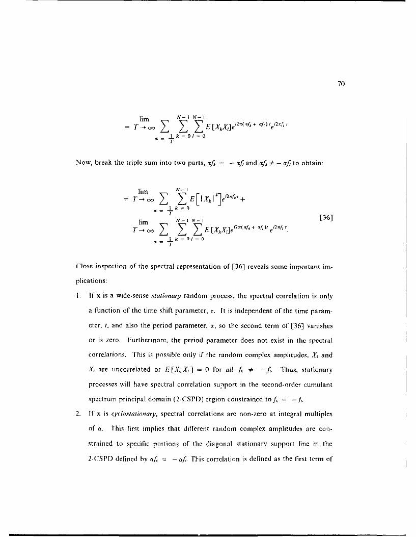
70

-+ z Y ErXkX]e21(efk+ - 2

I k 01 = 0CC T

Now, break the triple sum into two parts, af, = - f and orf #= - 4cf, to obtain:

im -

im I _ I[XkXI]ei2ff(1fA +l~<[6I - 0

Nir - I Iv- 1 [6]

a= I k =0/=1

T

(Close inspection of the spectral representation of [36] reveals some important im-

plications:

I. If x is a wide-sense stationary random process, the spectral correlation is only

a function of the time shift parameter, r. It is independent of the time param-

eter, t, and also the period parameter, a, so the second term of [36] vanishes

or is zero. Furthermore, the period parameter does not exist in the spectral

correlations. This is possible only if the random complex amplitudes. ,Yz and

X, are uncorrelated or E [X, XI] = 0 for all f, - -f, Thus, stationary

processes will have spectral correlation support in the second-order cumulant

spectrum principal domain (2-CSPD) region constrained tof, = -f,.

2. If x is cyclostationary, spectral correlations are non-zero at integral multiples

of a. This first implies that different random complex amplitudes are con-

strained to specific portions of the diagonal stationary support line in the

2-CSP[) defined by . - af. TFis correlation is defined as the first term of

71

[36] and has stationary characteristics. Periodic correlation components are

also created from the second term. These are a function of at and are off the

support set defined by a4, = - af, but rather are constrained to a support grid

in the 2-CSPD defined by: 4ck * - af. So, cyclostationary processes also

have nonstationary characteristics and provide a "bridge" between stationary

and nonstationary processes. In fact, cyclostationary processes are tractable

with generalizations of the tools used to study stationary processes (Cramer,

1960, Gardner and Franks, 1975, and lurd, 1989a and 1989b).

3. If x is nonstationary, non-zero spectral correlation may occur not only at inte-

gral multiples of at but rather for any t. Note that this general class includes

cyclostationary and stationary processes as a subset. Also, only the general

second-order cumulant spectrum representation captures spectral correlations

beyond the various support sets defined by f, = -fi, af, = - cf, and

caf, 7 - af. Correlated frequency components that are a function of any I

represent modulations of the purely periodic interacting components. Also, the

second term of [36] which has the periodic frequency components multiplied

by the sinusoid el2 f" also represent modulations and has support off the purely

cyclostationary grid (see Figure 3.1 on page 72). These modulated dependent

frequencies are proposed as more useful than single or coupled harmonic tones

in characterizing random incipient wear processes of rotating machinery.

It is shown how cyclostationary processes have both stationary and nonstationary

characteristics. More importantly, the investigation of a more powerful feature

characterization of periodic signal data for wear discrimination and classification

requires cumulant spectrum estimation. The 2-CSPI) region on wlich estimates are

computed for the joint random complex amplitude distribution is now developed.

72

SPECTRUMBROADENING

fl - 12

f2 pt-(p-)12

0 ~ pfi= (p-2)f2

p f p1 -(p-3)f 2

-, pf I -(P-4)f2

- ~ ~ - pf 1 - (p-5)f 2

0 -0 10 110pfl -(p4)f2

0 pfl -P8f

Stton\ Poe 1. -p7f2

(Disconinuous)(co1nt-nuou)s)

Figure 3.1:Powe Spectrum radngduet ouain- Sdbn

73

3.2.1. I Principal Domain Development

Without assuming weak stationarity the continuous, second-order cumulant

spectral representation of a stochastic process is:

CuM S (,f 2) = [ C 2(1 t 2 )e-12, (tfI + t 2 ) it1 dt2. [37]

This cumulant spectrum equation defines each estimated quantity over the entire

(f,fi) planar region. However, it is not necessary to compute the second-order

cumulant spectrum over this entire frequency plane as the Fourier transform pos-

sesses two important symmetry properties: permutation and conjugation. The

2-CSPID is defined as the minimum sl,ace on which second-order cumulant spec-

trum estimates are computed. The following four step process can describe the PI)

development for any order:

I. Apply permutation symmetry of Fourier transform (complex variates).

2. Apply conjugation symmetry of Fourier transform (real variates).

3. Combine permutation and conjugation symmetry operations.

4. Bandlimit and properly sample the process.

The 2-CSPI) is now developed with a corresponding graphical depiction.

Consider CumS_,, (.f,.f 2 ) as an estimate of the true second-order cumulant

spectrum which is based on the continuous Fourier transform of a large but finite

record length, T. of the process x:

A I

CumS (f ,2 )-- }E (f . [38]

74

Now consider CumS,, (f"f,):

A

CUM S. (f2 ,) - T Xf)Xf

= E {X(A) x(f2))A A

CumS. (f 2 J,) = CumS-, (f 2,).

Because of this permutation symmetry, a 450 line divides the entire (f,f2) plane into

two equivalent half-planes. See Figure 3.2.

f2o7

Figure 3.2: Complex Second-Order Cumulant Spectrum Principal Domain

Consider only thc right half-plane. The complex 2-CSPD is:

(fA,f 2 : -o 0 A oo,f 2 AA}.

Now consider Cum. , ( -f, -fi):

75

CuMS E[X( -f) X( -A))

-T E E{X'(fl) X*(f 2 )}T

A ACumS.( -f- 2 ) = _fmsj (f.,).

where - denotes the conjugate operation. This is the conjugation symmetry prop-

erty. It exists because for x a real-valued stochastic process, X( -f) = X4(f). So,

cumulant spectrum values in quadrants 1 (II) are equivalent to those estimates

computed in quadrant Ill (IV). Consider only quadrants I and IV. See

Figure 3.3.

f2III

Figure 3.3: Real Second-Order Cumulant Spectrum Principal Domain (1)

Thus, the 2-CSPD for a real-valued process is:

Now consider Cum.S,, ( -f, -f- ):

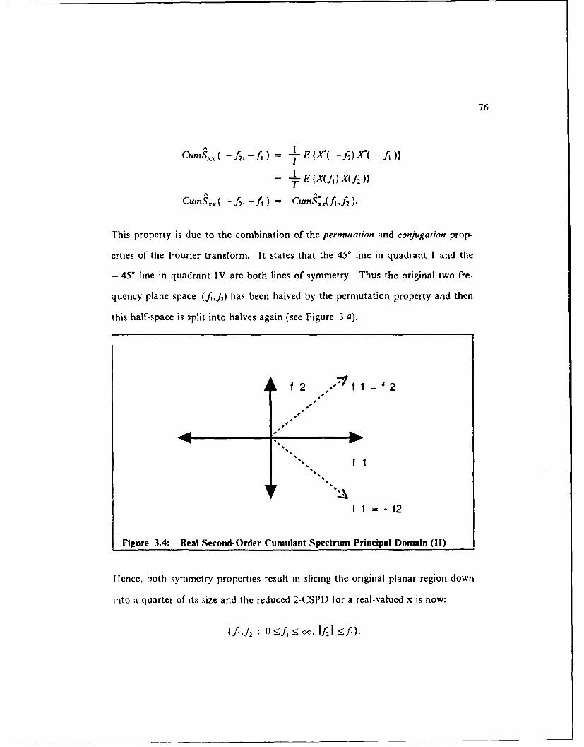
76

CUmS. ( -f 2A) - E( -f 2) Xr( -fA)TI E (X(A) X(f 2 )

-T

A 1

CuMS.( -A,- 1 ) = CumS.(A,f 2 ).

This property is due to the combination of the permutation and conjugation prop-

erties of the Fourier transform. It states that the 450 line in quadrant I and the

- 45' line in quadrant IV are both lines of symmetry. Thus the original two fre-

quency plane space (fi,fi) has been halved by the permutation property and then

this half-space is split into halves again (see Figure 3.4).

f 2 . " f1=f2

I-

fi1

f 1 f2

Figure 3.4: Real Second-Order Cumulant Spectrum Principal Domain (II)

Hence, both symmetry properties result in slicing the original planar region down

into a quarter of its size and the reduced 2-CSPD for a real-valued x is now:

(f,A • 0 <f < oo, 1f21 .A)

77

In actual implementation, the second-order cumulant spectrum is evaluated

numerically through a digital signal processing scheme. Hence, to satisfy the well-

known Nyquist sampling theorem, the stochastic process is bandlimited and sam-

pled at of least twice the highest frequency component, f,, to prevent aliasing.

Consequently, when the auto second-order cumulant spectrum is computed, it is

only necessary to compute estimates which reside in the triangular discrete 2-CSPD

region (see Figure 3.5) defined by:

(A 2 . < 21 !5 Af4}

ss'A

fc

'K\

f 1 -f2

Figure 3.5: Discrete Second-Order Cumulant Spectrum Principal Domain

The same rour step process can be applied to each succeedingly higher di-

mension. For the third-order cumulant spectrum:

CuM S (f,A 2 ,A) - J Jc= t2 '.2 t.)e - (t1f, + '2/2 + t3 f3) dt, dt2 dt3, [39]-- v0-a

78

each estimated quantity is defined over the entire (f,fi,fi) cubic frequency space.

However, estimates need only be computed in the discrete 3-CSPD region defined

by:

{ff 2 ,f3 : 0 < 1f3 I -<f2 -f1 -<fl}

The graphical depiction of principal domain regions in higher dimensions is more

difficult. Fortunately, a picture is not required by the computer to calculate the

estimates.

3.2.1.2 Estimation Procedure

This section describes the computational procedure to compute estimates

for the second-order cumulant spectrum (2-CS) from the direct discrete Fourier

transforms (DFTs) of finite record lengths. The procedure is basically an extension

of procedures for computation of traditional power spectra and it will be shown

that 2-CS estimates are computed from multiplying two discrete complex amplitude

spectral density functions. The same procedure can be followed for computing es-

timates for the third-order cumulant spectrum (3-CS) except that three complex

amplitude spectral density functions are multiplied and are computed over a differ-

ent principal domain region.

Begin with [38] which expresses CumS,. (fj,fi) in terms of expectations of

two rqn,'Im complex amplitude functions: X(f,) and X(f 2 ). Performing the ex-

pectation operation of random variables requires knowledge of an appropriate

probability density function which in most experimental studies is unknown. Thus,

ensemble averaging over a sequence of sample 2-CS is the approach for estimating

79

the expectation of the two complex random variables. Consider N identical inde-

pendent trials or runs of an experiment. Each run yields an outcome denoted by

x '(t), where k = 1, 2, ... , N. The collection of individual realizations defines the

ensemble of a particular stochastic process. If it is impractical or too costly to

gather a large number of realizations of a particular stochastic process by repeating

the experiment N times, there is another way to obtain more samples. If the time

duration of the original data record .s long enough, it may be subdivided into indi-

vidual frames of sufficient length to maintain independence and subsequently im-

prove the quality of the estimates. Of extreme importance with processing time

series data from periodic phenomena is definition of the frame length as an integral

multiple of the fundamental rotational frequency of the process being studied.

Also, another constraint when characterizing incipient faults is to capture at least

two fundamental periods. This is the lower bound as frequency resolution of sam-

pled estimates is given by Vf = l/T where T is the processed record length. Frame

lengths defined in this manner will capture modulations of the specified periodic

frequency which have been found to help characterize incipient wear states. No

data windowing techniques are needed to reduce the effects of leakage if an integral

number of periods or cycles are captured with the defined frame lengths.

So consider the set of N realizations or records for x, each record being T

seconds long. Each realization sampled with sampling interval i,, and consists of

N = Ilt, samples. T and N are determined from considerations previously dis-

cussed. Let x0l[n] represent the k', sampled realization and .Vi)[ I] the corre-

sponding DFT of xVA [n]. On the basis of [38], the appropriate estimate of the kh

sample 2-CS is:

80

cums~(f ,f) = I

Consider the values of the CFTs atf = 1Vf where Vf = liT. Then [38] becomes:

CumSxx(fII~f,2 ) = 1* '7 V)4T1 2 )'

Now, the sample values of the CFTs in terms of their respective DFTs are:

X k.(f [II [4IVf [41]

so expression of the continuous auto 2-CS in terms of its discrete auto 2-CS is:

k

Cutf.I I,,fl 2 ) = 2S[42]

Substituting [41] and [42] into [40] to obtain the sample discrete auto 2-CS:

CumS.)[ 11, 2 ] 12

vf 2 7- -' Vf

The final estimate of the discrete auto 2-CS is found by ensemble averaging over

all N realizations of the stochastic proces- studied:

N

CumS,[ 11, 12] = - N C"MSX[ 1,, 12]. [43]k= I

81

Note that if x = {x(:), t e N} is in volts, then the 2-CS estimate has the dimensions

cf volts2 and represents spectral components of two dimensional bandwidth cen-

te:ed at, and.( contributing to the mean square value of the stocha.tic process.

It is important t0 mention that estimates of succeedingly higher orders of

cur .lant spectra are found by a procedure similar to the one described for the

secc,',-, rd 'r case. The only difference is the number of DFTs being multiplied over

a correspor, n_'ly dimensioned PD region. Pseado-code for second-order cumulant

estilitation of cyclostationary time series is given below and the actual FORTRAN

program is at Appendix A.

Procedure Second-Order Cumulani Estimati,, i

Receive valid time series input parameters (# samples, sample rate, block length)

Load time series data into FFT work array

Calculate statistics (moments and cumulants) and subtract mean from data

While data blocks exist do

a) Subtract block mean from datab) Perform DFTc) Calculate Second-Order Cumulant Spectrum (double complex product)d) Accumi'late Chi-Squared Statistics over 2-CSPD

End Do

Output block summary statistics and correlations and Global Statistics

END

Valid parameters imply that sufficicnt working storage space is defined to

handle the amount of samples in the time series and also the chosen block length

is at least twice the fundamental frequency of the system. Two or more funda-

mental periods in a processed data block will calculate second-order cumulant es-

82

timates which correspond to intermodulation effects or nonstationary

characteristics of the random fault mechanism. Breaking the entire time series

record into proper block lengths is a method to increase estimation reliability by

decreasing estimate variability.

3.2.1.3 Reliability of the Estimates

Because of inter-machine variability, time series estimates of the

stochastic process under study are not perfect. Estimator quality is usually de-

fined by its bias and variance. Bias, b, is the difference in expected value of the

estimator and the "true" value:

A

b = EJ- ,

and so an estimator is unbiased if E[l] = 0. Variance is the spread in value

about the expected value:

A Apl= 72 E (0 EEC),]±E[1

A A A

= 2q E[ 20 12+]E[ 0+A2 2 A

So, estimator variance is equal to mean square value of the estimator minus the

square of the mean of the estimate. Now, consider mean square error which is

defined as the following and can be derived through expansion of the expectation

operation:

83

2 E[(^ 021 =(2 2.

Assume that the realizations are independent and that the process is ergodic.

Then with bar notation meaning expectation:

SXNcm 11 1 1,1t2]

Cum~CUM'x, 11, 12 1

NCumS[N12 = CurrSh)[ I, 2 ]

k = I

= 1 N-N NumSr'[l1 ,lI2 ]

= CumSx ,[ 1, 12 ].

and hence the estimator in [412] is unbiased. Also, [42] has a variance given by:

Var(Cumx[ 11, 12 ]} = C-1 11, -1-2

so that the variance decreases with the number of realizations. This agrees with

one's intuition that averaging of more realizations of random processes creates

better estimators.

Chapter 4

HOS Feature Extraction

4.1 Introduction

A feature extraction algorithm is developed to exploit the additional in-

formation provided by the power spectrum and the HOS transformations of raw

time series data. Several thousands of spectral estimates are usually generated for

a particular time series analysis application so a finite subset of the spectral esti-

mates, or features, are chosen from the entire collection of spectral measurements

to provide "optimum" classification results. There are three reasons for investi-

gating alternative estimation and feature extraction methods and evaluating their

classification results rather than using only one type of spectral analysis approach.

First, there is a cost for performing many different types of spectral estimation

procedures and their subsequent feature extraction. Actual computing time to

perform lOS estimation is not the most prohibitive factor; it is the feature ex-

traction process and subsequent classification that takes time and additional

computing. It is possible that power spectrum estimation and feature extraction

may provide sufficient classification performance for a particular application.

I lowever, performing I IOS estimation and feature extraction can be worthwhile

if it improves the overall classification performance of the power spectrum-based

approach. Proper I IOS transformations of the raw time series can lead to more

effective decision surfaces because of the more accurate representation of the

84

85

stochastic process structure being studied. Second, reducing the dimensionality

of the feature space eliminates redundancy as variables which do not add to the

classification accuracy are not included in the final decision rules. Third, a lower

misclassification rate is sometimes achieved by using fewer feature variables.

Further discussion of this topic is in the next section. The significant outcome of

the feature extraction process is the exposure of the individual spectral feature

variables and their combinations in measuring differences of multivariate popu-

lations. Thus, the HOS feature extraction approach is not only multivariate, but

also multispectral.

4.2 Features and Their Relationship to Misclassification Rate

Previous pattern recognition research observed for a given design set, in-

creasing the number of feature variables, d, causes classification performance to

initially improve, but then to deteriorate (Hand, 1981). This occurs because the

decision surface better fits the design set with increasing d but generalizes less well

to new samples since the design set became more sparsely distributed and less

representative of the class-conditional pdfs. Iland (1981) explains this phenome-

non using I lotelling's 7"2 statistic.

llotelling's 7" statistic, the distance between two sample means relative

to tile dispersion within the samples is:

2 n, 12 n, 12(VI - YV2)' V-1 - I) - ;

86

where .1, is the mean for class co,, V is the assumed common variance-covariance

matrix, and D' is the squared Mahalanobis distance measure defined in the back-

ground chapter. To investigate multivariate population differences, the question

asked is how often is T' observed as large or larger than the 7.2 estimated from the

samples if the two populations are identical? The statistical criterion value de-

fined by:

j =n-I-d 2

(n - 2)d

is compared with the F distribution with d and (n-l-d) degrees of freedom. If the

probability of a large T' is sufficiently low, one can conclude, with a certain risk

of error, that the populations are distinct.

Now, 7"2 changes as d, number of measurement or feature variables, in-

creases (Liddell, 1977). Consider each feature variable as independent of every

other feature variable and the standardized difference between the sample means

is some constant, k , for each variable. This allows D2 = k2d and thus:

J = (n - I - d)nln 2k 2dl(n - 2)dn

(n- I)nln2k2 ntn 2k 2

(n.-2) d .[44](n - 2)n (n - 2)n

[44] is a linear function of d, decreasing as d increases.

Van Ness and Simpson (1976) and Van Ness (1979) studied the rate at

which D2 must increase as d increases in order to maintain a constant or decreas-

ing error rate. They analyzed data from normal populations and compared three

parametric and two non-parametric classification algorithms. For each classifier,

87

they produced plots to determine the discriminatory power lost by increasing d

with D2 fixed, and how much D2 must increase in order to justify increasing d.

Their results showed that the non-parametric algorithms were quite stable at high

dimensions, and also outperformed the parametric algorithms at smaller dimen-

sions. Nevertheless, feature extraction is necessary to "squeeze" the most infor-

mation from a stochastic process with the least amount of variables. Some

existing feature extraction approaches were examined for use in this work.

4.3 Existing Feature Extraction Approaches

Algorithmic approaches for finding a feature space spanned by a subset

of the original measurement space are categorized into two major areas: selection

and transformation. Feature variable selection is appropriate if cost or other

factors present prevent all of the original set of features to be measured and used;

it is a combinatorial analysis problem. When all the variables can be measured,

variable transformation is performed but increased reliability occurs if a lower di-

mensional space is used. Variable transformation approaches include linear and

non-linear techniques. Both approach categories assume the number of potential

features is much less than the number of training samples. This was not the case

with experimental time series cases analyzed in this research. Consequently, a

hybrid approach was developed in this work. Before describing this hybrid ap-

proach, existing selection and transformation methods are given as some of their

aspects are incorporated in the IIOS feature extraction process.

Selection of a subset from the complete set of variables is approached

with exhaustive search, branch and bound, and stepwise methods. Exhaustive

88

search methods are only feasible when d is quite small. The major problem with

exhaustive search methods is how to test the many possible sets without the large

number of tests invalidating the significance level of each test. Branch and bound

algorithms accelerate the search of all variable sets but do not explicitly evaluate

all of them. Branch and bound is usually used on problems where the number of

possibilities evaluated increases exponentially with some fundamental parameter

of the problem. Unfortunately, even though branch and bound techniques slow

down the growth rate of possibilities, it remains exponential. Thus, suboptimal

search methods such as sequential forward selection and backward elimination

approaches are also used. Kittler (1978) gives empirical comparisons of these two

stepwise methods and extensions such as his generalized plus I-take away r se-

lection algorithm. This approach finds the particular 1-dimensional subset of

those variables not yet added which, when combined with the current set, leads

to the greatest J statistic [44]. Then each step examines the selected set to identify

those r variables, when discarded, reduce J by the least. His general conclusions

were that selection and backward selection methods which select/reject several

variables simultaneously were better than methods which select/reject one variable

at a time. Additionally, forward selection of two variables and backward deletion

of one variable gave the best results and was computationally favorable with

branch and bound methods. Since stepwise methods could continue indefinitely

if computation time is not a constraint, stopping criteria such as a test statistic

given by Rao (1970) tests whether an extra (d-d') variables makes a significant

contribution to the discrimination task.

Variable transformation methods include canonical discriminant analysis

(CI)A) which finds a set of axes spanning a subspace of the complete space where

89

class separability is maximized. CDA is done in a similar fashion as principal

component analysis (PCA) for summarizing total variation. But, with PCA, only

one data set is analyzed, while CDA analyzes at least two data sets. PCA also

subtracts means so it is an analysis of variance/ covariance. CDA also does a

PCA of class variable means. Variables used for canonical discriminant compu-

tation need to have an approximate multivariate normal distribution within each

class and a common covariance matrix. However, a linear discriminant boundary

may be determined by a least squares argument without the assumption of

normality and common dispersions of the two parent distributions (Kendall et al.,

1983). If it is the case that the multivariate normality assumption is unjustified,

non-linear feature extraction methods have also been developed (Fukunaga and

Ando, 1977).

4.4 New Hybrid Approach

When the number of potential feature variables is much greater than the

sample si7e, a hybrid approach that attacks such problems in stages is necessary

(Jain and Dubes, 1978). The HOS feature extraction algorithm is composed of

three stages. First, visual plots of ensemble averaged spectra and their differences

between groups are generated after each respective spectral estimation process to

obtain a rough idea of which estimates to use as possible feature variables. This

is the graphical variable selection stage. I linich and Clay (1968) describe the gen-

eral procedures followed for frequency domain estimation of a time series record.

The statistical tests oflinearity and (Gaussianity of a time series (Ilinich, 1982) are

extended For use with second-order cumulant spectrum estimates. The modulus

90

of the second-order cumulant spectrum and bispectrum estimates are statistically

transformed to chi-square values for subsequent use as feature measurements.

Hinich (1989) describes the statistical transformation process for bispectra moduli.

All types of spectral estimates are ensemble averaged for the frequency variates

of the particular spectral function after estimation of all time series records used

for training function computation is performed. Second, univariate analyses of

variance are performed and the resulting F-statistics are plotted for the corre-

sponding frequency principal domains of each spectra type to confirm visual dif-

ferences seen in the ensemble averaged plots. Spectral variables shown to be good

candidates for the feature set are selected based on their F value. Only the top ten

of each spectra type are chosen as potential feature variables. This second stage

is a dimension reduction step to reduce each individual spectral space to represen-

tative variables. Third, a conventional variable selection algorithm. stepwise se-

lection of variables available in SAS 6.0,1 a statistical analysis software package,

is applied using the thirty spectral variables identified from the second stage.

Stepwise discriminant analyses are performed to obtain the best linear (power

spectrum) discriminators, the best nonstationary (second-order cumulant spec-

trum), the best quadratic (bispectrum) discriminators, the best linear and nonsta-

tionary discriminators, etc., so the important relationships of the reduced and

combined spectral feature space are considered. The "optimum" individual spec-

tral feature sets composed of ten potential feature variables, either power spec-

trum, bispectrum, or second-order cumulant spectrum feature sets, are found to

be average discriminators by themselves. However, when the different spectral

SAS is a registered trademark of the SAS Institute, Inc.

91

feature sets are combined according to certain statistical criteria, their discrimi-

nation and classification power significantly increase (see Chapter 5).

This hybrid feature extraction approach generates ensemble averaged

plots, F-test plots, and "optimum" feature sets. Once feature extraction for the

various types and combinations of spectra is complete, marginal and sensitivity

studies are conducted on simulated and actual time series to test and evaluate the

different approaches.

Before the 11OS feature sets are presented and discussed for the simulated

and actual experimental data, statistical test results of raw time series from the

actual wear database are given. Bispectrum statistical tests are employed to in-

vestigate if the observed time series records are consistent with the hypothesis that

the underlying stochastic process has a Gaussian distribution, and whether the

process contains evidence of nonlinearity in the underlying physical mechanisms

generating the observed vibrations. The sample bispectrum is the two dimensional

Fourier transform of the expected value of the vibration signal at three time

points, and should be a standardized normal random variable if the process is

stationary, linear, and Gaussian (Itinich, 1982). Shown at Table 4.1 on page 92

and Table 4.2 on page 92 are the results from applying the Ilinich linearity and

gaussianity tests to the two bt classes for each stack/load time series.

92

Table 4.1

Gaussianity and Linearity Test Statistic Results For New Bits--Actual Wear Ex-periment. The Z statistic is a normal approximation of the central chi-squaredvariate with large degrees of freedom. It is a N(0,1) random variable under the nullhypotheses of a Gaussian and a linear process.

Time Series Gaussianity Statistic (Z) Linearity Statistic (Z)(Stack/Load) Mean Std Mean Std

NIP/3 54.2 39.7 54.8 42.4

NIP/4 356.4 212.9 367.2 216.2

6S2P/3 40.8 32.1 40.2 35.8

6S2P/4 186.9 183.9 192.4 189.4

Table 4.2

Gaussianity and Linearity Test Statistic Results For Slightly Used Bits--ActualWear Experiment. The Z statistic is a normal approximation of the central chi-squared variate with large degrees of freedom. It is a N(0,1) random variable underthe null hypotheses of a Gaussian and a linear process.

Time Series Gaussianity Statistic (Z) Linearity Statistic (Z)(Stack/Load) Mean Std Mean Std

NIP/3 105.4 67.4 108.4 69.3

NIP/4 358.7 326.1 367.0 332.4

6S2P/3 56.8 43.9 56.5 47.9

6S2P/4 237.3 229.3 229.9 192.8

These global test statistics show that the drill spindle vibration time series

for the Z accelerometer are definitely non-Gaussian and nonlinear for both new and

slightly uscd drill bits. Also, the ensemble averages and standard deviations of

both statistical measures are higher For slightly used bits than new bits. Possibly.

the increased nonlinear and non-Gaussian structure of slightly used bit spindle

93

vibrations are due to bit wear mechanisms such as flank or rake wear changing the

geometry of the bit cutting surface and causing the thrust forces to increase.

Possibly incipient bit wear causes more significant frequency coherence at certain

frequency components. Also Table 4.1 on page 92 and Table 4.2 on page 92 re-

veal as more panel stack material is cut with each revolution of the drill (4 mil/rev

versus 3 mil/rev), higher statistical values are obtained which correspond to the

increased "strength" of the interacting frequency components. Thus, these global

statistical measures are corresponding to the actual physics of the circuit card

cutting process.

4.5 Results

Even though th -lobal I linich statistical measures are indicative of class

distinguishability, feature extraction emphasis is on the statistical selection of

particular linear, nonstationary, and nonlinear spectrum estimates for subsequent

input to an efficient classification algorithm. The ultimate aim is to reveal features

of a consistent relationship that have good classification performance. The se-

lected features can then potentially providc a deeper understanding of the physics

of a particular physical process under study. I fence, the desired properties of ex-

tracted features in order of priority are:

1. consistent classification performance.

2. physically interpretable with some correspondence to the physics of the

stochastic process, and

3. good visual discrimination ability,

94

Feature extraction results are given generally for the simulation scenarios

and then details for all the database partitions of the actual experiment are given

in tabular format. (The simulated and actual wear experiments are described in

Chapter 5). Feature extraction results will confirm the research hypothesis that

I IOS features, and particularly estimates of the second-order cumulant spectrum

not part of the purely periodic support grid within the 2-CSPI) region provide

better features for incipient wear characterization.

Simulation feature extraction results for all the scenarios (see 'Fable 5.1

on page 115) are summarized as particular frequency values do not have any

physical meaning. The final IIOS extracted feature sets for all simulated scenarios

were composed of twenty-eight power spectrum, fifty-one bispectrum, and

twenty-five cumulant spectrum feature variables. For each particular scenario, the

number of ItOS features was larger than the number of power spectrum features

and had a higher star: * al significance level. Most significantly, twenty-one of the

twenty-five, or 84 percent, of the second-order cumulant spectrum variables were

off the pure cyclostationary support grid in the 2-CSPD. These features were also

in the middle to highest ranges of statistical significance with relation to the other

features selected. Thus, evidence from simulations weighs in favor that incipient

wear characterization is enhanced by performing cumulant spectrum estimation

and feature extraction. The real test of the hypothesis will ie examination of

eature extraction results from actual wear data.

Visual inspection of each type of ensemble averaged spectral plots for the

two classes of drill hits give a preliminary look of whiclh frequency variatcs are bit

class distinguishable. See Figure 4.1 on page 96 and Figure 4.2 on page 97 for

ensemble averaged power spectrum plots and ensemble averaged bispectrum

95

chloropleth plots for new drill bits for a particular case of the actual wear data

described in Chapter 5. Also, see Figure 4.3 on page 98 and Figure 4.4 on page

99 for ensemble averaged power spectrum and ensemble averaged bispectrum

plots for slightly used drill bits of the same case.

These individual plots, Figure 4.1 on page 96 and Figure 4.3 on page

98, and Figure 4.2 on page 97 and Figure 4.4 on page 99, of the different drill bits

are combined so that differences in spectrum estimates for the two groups are

more visually apparent. See Figure 4.5 on page 100 and Figure 4.6 on page 101

for representations of the differences in ensemble averaged power spectrum and

ensemble averaged bispectrum.

Overlaying the representations of the two ensemble power spectrums and

their variability serves its purpose as a preliminary look at what range of fre-

quencies are bit class distingui.hable. Differences in ensemble averaged power

specti um plots for all four stack/chip load cases were quite similar as that shown

in Figure 4.5 on page 100. Power spectra exhibited the presence of strong spec-

trum peaks at frequencies below 5 kllz. These peaks occurred at the shaft spindle

rotational frequency, f,, and its harmonics, 2f, and 4f, and reflect the periodic

cutting forces due to hardness differences of the glass anad epoxy material in the

circuit card layers. Most of the signal content occurs at the harmonic frequencies

and dn not appear useful as outstanding wear indicators. Ilowever, there are two

frequency ranges which visually appear useful as potential wear indicators: fre-

(quiency values near one-half the fundamental rotational frequency of the drill

spindle, .5f, and between 14-14.5 kllz. Other researchers have noted this sub-

harmonic structure with journal bearings in high-speed turbomachinery, some-

times referring to it as a whirl frequency (Braun, 1986). This may be due to less

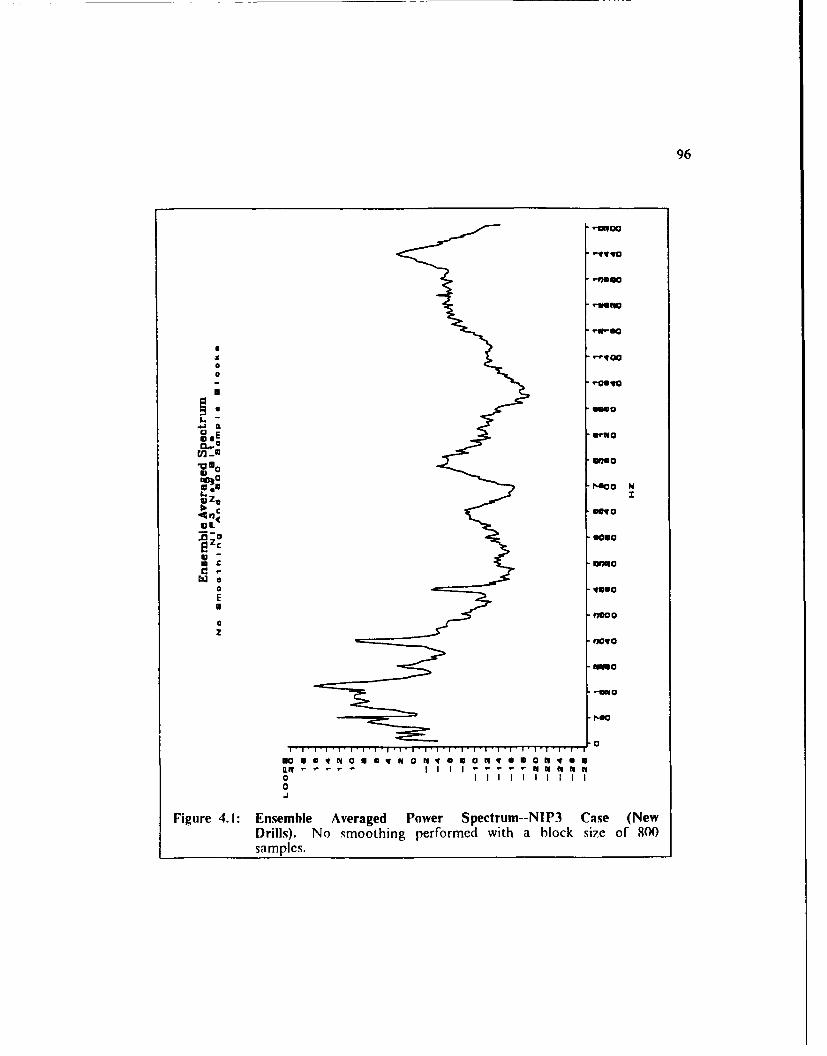
96

-moo

-MOO

-VOO

0

C-000

in --0ii

M 100 N

Ux

"000

Z.Z

I--.

O~MMU

"fl -, ~l

43~3

rjIloo

1000

66t

.J

Figure 4. 1: Ensemle Averaged Power Spectrum--NIP3 Case (New

Drills). No smoothing performed with a block size of 800samples.

97

Ensemble Averaged Chi-Square StatisticsOver Bi-Frequency Plane

For Nip Stock Chip Lined 3 Eil/Row

For New Bits

rRE02

145 17

548

784 7811 148199 21915 29033.

FRE01

CHISOAVE 0 2 4

Figure 4.2: Ensemble Averaged Bispectrum--NIP3 Case (NewDrillsi). Ensemble averaged chi-square statistical measures aretransformations of bispectra moduli or squared gain. Legenddefined shows the magnitude of the chi-square statistic denotingfrequency interaction strength. No smoothing performed with asample block size required to capture two integral periods of theprocess.

98

-- V 00

u 0

000

lu ni -Mo

nwuo

IIM

003

mari

Fiur 4-:E1U60AvrgdPwrSpcrmNP as(lgtyUe

Drls.NEmohn efrmd wt lc ieo 0sa pls

99

Ensemble Averaged Chi-Square StatisticsOver Bi-Frequency Plane

Fir NIP Stock Chip Load 3 Nil/Rev

For Slightly Used Bits

FREQ219101

14517

9933

5348

764

784 7831 14199 21966 29033

FRE01

CHISOAVE 0 2 M 4L"-' 6 a ImlnfMl l0

Figure 4.4: Ensemble Averaged Bispectrum--NIP3 Case (Slightly UsedDrills). Ensemble averaged chi-square statistical measures arctransformations of bispectra moduli or squared gain. Legenddefined shows the magnitude of the chi-square statistic denotingfrequency interaction strength. No smoothing performed with asample block size required to capture two integral periods of theprocess.

100

-_..Woo

I-L

0" .T.-. " ll'

r. l-

Z V el

_: N~.43a

UZO

0

Figiire 4.5: Ensemble Averaged Power Spectrum Differences-- N IP3Case. New bit ensemble average is denoted by squares andslightly used bit ensemble average by circles. Small dashes are 95

percent confidence limits for new and larger dashes are those forslightly used. No smoothing performed with a block size of 800samples.

101

Difference of Ensembled Averaged Chi-Square StatisticsOver III-I requesay Piae

rof NIP Stock Chip ioad 3 Mi i/RovIletmes New Bits and slightly Used Bits

FRE0218337

13944

9551

5157

*5 4

784 78.31 14899 21955293

FRE0O1

OCHIAVE 0 C82 24 5 5

Figure 4.6: Ensemble Averaged Bispectrum Differences- N IP3Case. Differences in ensemble averaged chi-square statisticalmeasures are transformations of bispectra moduli or squared gain.Legend defined shows the magnitude of the chi-square statisticaldifferences of frequency interactions. No smoothing performedwith a sample block Si7e required to capture twvo integral periodsof the process.

102

frictional forces of a slightly worn drill bit. The higher range of frequency values

are near a torsional resonant frequency of the drill spindle. As the top portion of

the spindle rotates in one direction, its body rotates the opposite direction (see

Figure 5.3 on page 127). The spindle rotation causes the drill bit to slightly go

up and down during the drilling process. It appears the spindle torsional mode is

more strongly excited by new drills than slightly worn drills. A decaying torsional

oscillation excited by contact of worn cutting surfaces of the drill is physically in-

tuitive.

The bispectrum difference chloropleth plots clearly show the general re-

gions and the particular frequency interaction pairs that are class distinguishable.

Differences in ensemble averaged bispectrum chloropleth plots for all four

stack/chip load cases are similar to Figure 4.6 on page 101. Differences of en-

semble bispectrum chi-square values first show drill class distinguishability in fre-

quency interaction regions composed of first through the eighth harmonics of the

fundamental rotational frequency of the drill spindle with frequencies greater than

14 kllz. A portion of this significant different frcquency struLture may be due to

parametric coupling of the torsional resonant frequency with each of its lower

harmonics. This fact is significant as Ramirez (1991) discovered from his analysis

of extended drill wear data that the fifth through the eighth power spectrum har-

monics of the same accelerometer (Z or thrust axis) are the most sensitive drill

wear indicators. Thus, a predictive capability may have been demonstrated with

bispectrum analysis of the incipient wear data. Also significant is that for all the

stack/load cases, bispectrum estimates are most significantly difTercnt in the outer

triangle (OT) region of the birpectrum principal dnmain. This was evidence and

motivation for further investigation with cumulant spectrum estimation and fea-

103

ture extraction as it meant the existence of a nonstationary generating source in

the stochastic process (Hlinich, 1989).

Extracted second-order cumulant spectrum features were consistently not

on the pure cyclostationary support grid in the 2-CSPD which confirms the major

theoretical proposition stated in Chapter 3. Furthermore, they were always the

most significant feature variables for all but one of the eight actual wear database

partition cases (NIP4). Significantly, the NIP4 is the only database partition

where no overall marginal improvement in discrimination and classification power

was obtained by incorporating HOS feature information. This Fact adds further

evidence that better incipient wear characterization is provided with 2-CSPD es-

timates off the cyclostationary support grid. Consider the following physical ex-

planation why these statistical correlations discovered by the feature extraction

algorithm are most important. Cards were manufactured in the same facility with

the same resin system but had different glass cloth and layer thicknesses. See

Figure 4.7 on page 104 for two examples of card construction. Biecause the glass

fibers (oval disks in diagram) cut during each hole are not uniformly configured

in the card layers, the vibration signals will have periodic and aperiodic charac-

teristics and reflect the effects of many different cutting geometries randomly en-

countered by the drill. So the cutting forces and energy represented by the

vibration measurements change within a certain layer of the card and also for each

revolution of the drill. Vibration measurements carrying wear information of the

drill cutting edges will thus he more sensitive to spectral correlations that are not

integer multiples of the fundamental rotation of the drill spindle. Extracted fea-

tures shown in the following tables reveal the importance of second-order

cumulant estimation.

104

Jy 1.52mm 1.22 mm

Figure 4.7: Circuit Card Construction

Table 4.3

Actual Experiment Feature Extraction--NIP/3 Case. Scum denotes the second-order cumulant spectrum, Bisp denotes the bispectrum, and Spec denotes the powerspectrum. Feature variables are listed in the order entered by the SAS variable se-lection algorithm. Cyclic frequency of the drill spindle is 764 Hz.

Frequency Spectrum F-Stat Off 2-CSPI)Value (Hz) Type Value Periodic Grid?

9550,1910 Scum 16 yes12224,1528 Scum 13 no

6876,8404 Bisp 8.5 n/a

14520 Spec 7.6 no764,11460 Bisp 5.4 n/a1528,15281 Bisp 6.7 n/a

8608 Spec 7.9 yes

13290 Spec 3.0 yes

13190 Spec 4.2 yes

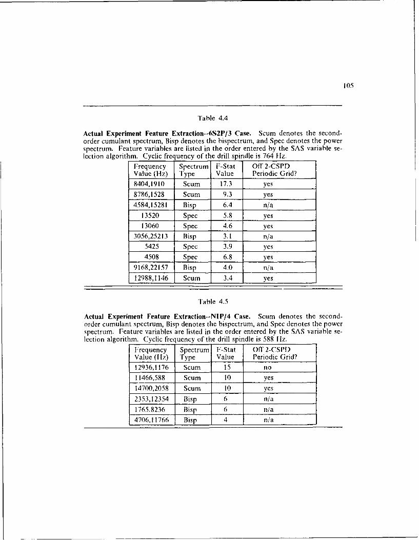
105

Table 4.4

Actual Experiment Feature Extraction--6S2P/3 Case. Scum denotes the second-order cumulant spectrum, Bisp denotes the bispectrum, and Spec denotes the powerspectrum. Feature variables are listed in the order entered by the SAS variable se-lection algorithm. Cyclic frequency of the drill spindle is 764 Hlz.

Frequency Spectrum F-Stat Off 2-CSPDValue (Hz) Type Value Periodic Grid?

8404,1910 Scum 17.3 yes

8786,1528 Scum 9.3 yes

4584,15281 Bisp 6.4 n/a

13520 Spec 5.8 yes

13060 Spec 4.6 yes

3056,25213 Bisp 3.1 n/a

5425 Spec 3.9 yes

4508 Spec 6.8 yes

9168,22157 Bisp 4.0 n/a

12988,1146 Scum 3.4 yes

Table 4.5

Actual Experiment Feature Extraction--NIP/4 Case. Scum denotes the second-order cumulant spectrum, Bisp denotes the bispectrum, and Spec denotes the powerspectrum. Feature variables are listed in the order entered by the SAS variable se-lection algorithm. Cyclic frequency of the drill spindle is 588 l Iz.

Frequency Spectrum F-Stat Off 2-CSPDValue (I lz) Type Value Periodic Grid?

12936,1176 Scum 15 no

11466,588 Scum 10 yes

14700.2058 Scum 10 yes

2353,12354 Bisp 6 n/a

1765.8236 Bisp 6 n/a

4700,,11766 Bisp 4 n/a

106

Table 4.6

Actual Experiment Feature Extraction--6S2P/4 Case. Scum denotes the second-order cumulant spectrum, Bisp denotes the bispectrum, and Spec denotes the powerspectrum. Feature variables are listed in the order entered by the SAS variable se-lection algorithm. Cyclic frequency of the drill spindle is 588 lHz.

Frequency Spectrum F-Stat Off 2-CSPDValue (I tz) Type Value Periouic Grid?6468,1470 Scum 9.1 yes9413,10589 Bisp 7.7 n/a

12870 Spec 3.6 yes

2574 Spec 4.3 yes14494,2352 Scum 4.5 yes

6471,8824 Bisp 6.2 n/a12642,1764 Scum 3.2 yes

9702,1470 Scum 4.0 yes

Table 4.7

Actual Experiment Feature Extraction--Combined Load 3 Case. Scum denotes thesecond-order cumulant spectrum, Bisp denotes the bispectrum, and Spec denotesthe power spectrum. Feature variables are listed in the order entered by the SASvariable selection algorithm. Cyclic frequency of the drill spindle is 764 liz.

Frequency Spectrum F-Stat Off 2-CSPDValue (Ilz) Type Value Periodic Grid?

8404,1910 Scum 36 yes

13370,12988 Scum 11 yes

3056,9932 Bisp 6.0 n/a

14870 Spec 4.5 yes

6876,11460 Bisp 5.4 n/a

6112,12988 Bisp 4.4 n/a

1528,1528 Bisp 3.6 n/a

8455 Spec 4.4 yes9550,1910 Scum II yes

107

Table 4.8

Actual Experiment Feature Extraction--Combined Load 4 Case. Scum denotes thesecond-order cumulant spectrum, Bisp denotes the bispectrum, and Spec denotesthe power spectrum. Feature variables are listed in the order entered by the SASvariable selection algorithm. Cyclic frequency of the drill spindle is 588 ltz.

Frequency Spectrum F-Stat Off 2-CSPIDValue (1Hz) Type Value Periodic Grid?9702,2646 Scum 13.5 yes

4410,1176 Scum 8.5 yes

12642,1764 Scum 4.9 yes

7060,11178 Bisp 5.0 n/a

9702,294 Scum 4.2 yes

8236,11178 Bisp 5.0 n/a

14494,2352 Scum 5.3 yes

9354 Spec 4.4 yes

10589,13531 Bisp 5.3 n/a

7648,12354 Bisp 2.8 n/a

Table 4.9

Actual Experiment Fe"Iure Extraction--Combined Stack NIP Case. Scum denotesthe second-order curlulant spectrum, Bisp denotes the bispectrum, and Spec de-notes the power spectrum. Feature variables are listed in the order entered by theSAS variable selection algorithm. Cyclic frequency of the drill spindle is 588 l Iz and764 lIz.

Frequency Spectrum F-Stat Off 2-CSPDValue (I z) Type Value Periodic G. id?9408,2058 Scum 7.2 yes

9413,17061 Bisp 5.9 n/a

588,6471 Bisp 3.6 n/a

7060,15296 Bisp 3.5 n/a

12348,1470 Scum 3.5 yes

13530 Spec 3.8 no

108

Table 4. 10

Actual Experiment Feature Extraction--Combined Stack 6S2P Case. Scum denotesthe second-order cumulant spectrum, Bisp denotes the bispectrum, and Spec de-notes the power spectrum. Feature variables are listed in the order entered by theSAS variable selection algorithm. Cyclic frequency of the drill spindle is 588 Hz and764 lIz.

Frequency Spectrum F-Stat Off 2-CSPDValue (liz) Type Value Periodic Grid?8232,2058 Scum 36.0 yes

8820,1470 Scum 20.0 yes

2941,7648 Bisp 13.5 n/a

12642,2352 Scum 10.5 yes

1765,8236 Bisp 10.4 n/a

588,13531 Bisp 8.4 n/a

8236,10589 Bisp 5.6 n/a

13160 Spec 5.3 yes

4706,16472 Bisp 5.0 n/a

12870 Spec 4.6 yes

12936,1176 Scum 4.4 no

13240 Spec 3.7 yes

The evidence of IOS feature extraction of actual incipient wear data

clearly supports that IIOS features are significant in the feature sets extracted to

define class differences. Additionally, the theoretical proposition of second-order

cumulant spectrum estimates off the periodic support grid as those which better

characterize incipient faults ofcyclostationary processes is confirmed. Now, what

remains is an investigation of the impact of the extracted I IOS features on classi-

fication performance, using various multivariate classifiers under different process

conditions, to test the robustness of the new incipient fault detection approach.

Chapter 5

Evaluation of HOS Approach

5.1 Introduction

Performing discrimination and classification tasks on simulated and actual

time series data generated from processes that have cyclostationary characteristics

comprises the test and evaluation of the new I IOS incipient fault detection ap-

proach. Factorial designs, data collected, and principles behind the experiments

are described and then the discrimination and classification results using different

feature extraction sets are given. Probability of false alarm and probability of

detection are the measures of effectiveness used to evaluate the r ,lative merit of

the various approaches.

5.2 Simulated Wear Experiment

Modulation theory describes how a pure deterministic signal emitted by

a periodic force is transformed into a signal actually measured by a condition

monitoring system. Consider modulation as a mapping of the driving force signal

space to the measurement signal space. Some possible mapping factors are : (I)

internally and externally generated noise, (2) structural propagation, (3) change in

process state, and (4) change in process environment. The transformation of an

original driving force signal is equivalent to a translation of spectra. A pure sine

109

110

wave tone is a delta function or a single spike in spectral representation. A change

in process environment (i.e. cutting forces required to cut through various

strengths and types of material) will cause variation in frequency and amplitude,

but the spectral components which specify the cutting force process dynamics are

translated without any change to their relative energy distribution--the peak

magnitude is decreased but the sidebands correspondingly increase to compensate

the energy loss. However. a change in process state will cause variation or mod-

ulation of phase which will generate new frequencies with a different energy dis-

tribution of the signature signal spectral components. Parameters of the

simulation experiment emphasized changes in phase, rather than changes in am-

plitude, and its impact on classification/feature extraction performance for several

sets of process state and process environment parameters.

When the driving force of a physical system is periodical (eg., in rotating

machinery), the signature signal emitted by the process and received by sensors

may be represented by a harmonic process (Priestley, 1986). Consider a rotating

drill machine and the process of cutting holes in electronic circuit cards which is

the actual wear experiment analyzed later in this chapter. Assume the signature

signal is a vibration time series sensed by accelerometers. The harmonic process

model (11PM) in this case is:

-- A, cos(2,rn t + 0,) + n(t) [45]n=0

where V(t) is the voltage of the cosine wave carrier signal, A and 4) are the am-

plitude and phase terms oF the driving force mechanism (drill rotation) or carrier

signal; f. is the fundamental carrier frequency determ*ned by the period of the

Ill

driving force function and vibration characteristics of the machine system; and

n(t) is the corrupting noise generated by other vibratory sources and distortional

effects. Noise is assumed Gaussian and independent to the emitted vibration sig-

nal and k is the number of interacting sinusoids. Thus, the observed periodic

voltage time series record is described by sums of sine and cosine waves whose

amplitudes and phases are chosen to give the best fit to the observational data.

The decomposition of the periodic time signal is found by obtaining the Fourier

series of the time series record.

If {fq,, n = 0, I, 2, ... ) are identical and independent uniformly distributed

variables on ( - 7t, r), { V,(t), t > 0) is stationary no matter what frequency and

amplitudes are selected to represent the voltage time series. Furthermore, both

the autocorrelation and autocovariance functions of a I1PM consist of a sum of

cosine terms and therefore never die out in contrast to moving average (MA) and

autoregressive (AR) processes. Thus, finite dependence or finite memory where

joint random variables are highly correlated when the time instants are close to-

gether, and low correlation when the time instants are widely separated, is not

applicable to a 11PM representation of stochastic processes. (see Appendix B for

stationarity of 11PM and inapplicability of finite memory).

In this discussion, consider the cosine-wave carrier signal as referring to

[45]. Its amplitudes, A,, and phases, 4,,, can be varied according to modulating

or infrmation signals representing physical wear processes. The cosine-wave

carrier signal is amplitude and phase modulated once the rotating drill begins to

wear due to its drilling holes in electronic panels. The inherent energy will fluc-

tuate, or he amplitude modulated, due to the change in (trill bit surface contact

pressure and force at each cutting revolution because of differences in hardness

112

and thickness of panel materials. Additionally, as more holes are drilled over time,

the drill bit cutting edges will wear and cause phase modulation of the baseline or

reference (no wear) voltage signal. Consider the situation where k is just I.

The cosine-wave carrier signal, [45], or the inherent energy of the rotating

drill spindle is amplitude modulated due to its periodic nature. A cosine wave with

fluctuating amplitude is also known as the phenomenon of beats. By superim-

posing two cosine waves with nearly equal frequencies, co + bco, the result is:

cos(co + co)t + cos(ao - bco)t = 2 cos cot cos .5wt.

This oscillates at the average frequency, o = 2nf, but the amplitude changes

slowly according to the modulating function, 2 cos &5wt. So the amplitude modu-

lated version of[45] where the time icference is chosen so the carrier phase angle

is zero is:

Vam(t) = k[l + rnft)] cos(coct) + n(t).

Multiplying fit) = 2 cos .wt by cos(ot) causes a spectrum shift up to a range of

frequencies surrounding the carrier frequency, f, and the addition of the carrier

term provides a discrete spectral line at frequency f. These range of frequencies

are sometimes called the lower and upper sidebands where each sideband contains

amplitude and phase information of the original sinusoidal signal. Amplitude

modulation is not the only method of modulating a cosine-wave carrier.

Consider a frequency modulated system in which the frequency of the

carrier is caused to vary in accordance with some type of information-carrying

signal. This could he variations in the bit cutting forces due to rake and flank

wear and minor rpeed fluctuations of the drill spindle as it wears over time. The

113

frequency of the sine wave carrier is (o. + kJ(t) with fit) representing the phase

modulating signal and k is a system constant. Expressing the more general fre-

quency modulated carrier in mathematical terms is difficult because one can define

the frequency of a sine wave only when the frequency is a constant. Strictly

speaking, there is only the sine or cosine of an angle. However, if the angle varies

linearly over time, one can interpret the frequency as the derivative of the angle:

f,(t) = cos 0(t) = cos(Gw't + 0').

If 0(t) does not vary linearly, the instantaneous radian frequency wo, is the deriva-

tive of the angle as a function of time:

dO= cos 0(1); w .= d-

This now agrees with the usual use of frequency if 0 = wjt + 0,.

I lence, the rotating drill spindle does not generate a signal that is a pure

harmonic tone, cos 2tft = cos oj, but rather is an amplitude and phase modu-

lation representation of [45]:

Vanpm(t) = k[l + mat)] cos(',t + ), 4- mrg(t)) + n(t) [46]

where V,,(t) is the amplitude and phase modulated cosine-wave carrier signal,

n. is the amplitude modulation index, flt) is the amplitude modulating signal, 4,

is the carrier signal phase, m, is the phase modulation index, and g(t) is the phase

modulating signal. Now, fit) = cos ,),t and g(t) = cos int with f, and f, being the

frequency of the amplitude and phase modulating wave, respectively.

Consider both amplitude and phase modulations modeled by:

114

N-!

Vamp,(t) =k=O

lence, a zero-mean random fluctuation vibration signal made up of a sum of N

complex sinusoids with each frequency being described by complex amplitude A

has zero complex mean when there is no modulation. Once wear progresses, these

complex amplitude signals contain both random amplitude and phase modu-

lations which result in broadening of their bandwidth or a correction to the pure

line spectrum, and A becomes a nonzero complex random variable. If mSt) and

mg(t) are zero mean, stationary, and statistically independent, the power spectral

density of V,(t) can be derived to show how the presence of random amplitude

and phase modulations produce bandwidth broadening (see Appendix C). The

primary interest for incipient fault detection is classifying changes in the phase

modulation index parameter of the signature signal that corresponds to the degree

of wear or developing failure in a rotating machine process. Details of the simu-

lation experiments are given next.

Two hundred and fifty independent classification runs using three alter-

native feature extraction methods for fourteen treatments, or incipient failure

cases, were performed. Three simulation parameters or factors are changed in a

most deliberate fashion to represent fourteen very difficult

discrimination/classification problems. These parameters are amplitude and phase

modulation indice values, and standard deviation of an independent Gaussian

noise term. The fourteen treatments can be logically categoried as seven rce-

narios shown at Table 5.1 on page 115. Fach scenario has two treatments with

a correspondingly increased value in phase modulation associated with a fixed

115

level of amplitude modulation and independent Gaussian noise standard devi-

ation. Thus, each treatment entry of Table 5.1 on page 115 is a discrimination

and classification problem of two classes of two hundred and fifty simulated time

series.

Table 5.1

Seven Incipient Fault Detection Scenarios--Simulated Wear Data. Each scenariohas two discrimination/classification cases. Numbers in parentheses are the simu-lation parameters: amplitude modulation index, phase modulation index, andstandard deviation of Gaussian noise.

Scenario ClassificationNumber Treatment

IA (.3,.7,4) vs (.3,.71,.4)

lB (.3,.7,4) vs (.3,.72,.4)

2A (.3..7,.8) vs (.3,.71,.8)

2B (.3,.7,.8) vs (.3,.72,.8)

3A (.3,.7,1.4) vs (.3,.71,1.4)

3B (.3,.7,1.4) vs (.3,.72,1.4)

4A (.3,.4,.4) vs (.3,.41,4)

4B (.3.4,4) vs (.3.42,.4)

5A (.3,.4,.8) vs (.3,.41,.8)

5B (.3,.4,.8) vs (.3,.42,.8)6A (.3,.4,1.4) vs (.3,.41,1.4)

6B (.3,.4,1.4) vs (.3,.42,1.4)

7A (.5,.7,.4) vs (.5,.71,4)

7B (.5,.7,4) vs (.5,.72,4)

Standard International Mathematical Statistical L.ibrary (IMSI-) routines were

used to generate Gaussian noise and deterministic phase. L.evels for amplitude

modulation were considered fixed as it represents more of a change in environ-

ment rather than a change in process state; however, amplitude modulation was

116

changed for sensitivity and verification purposes. There were three phase modu-

lation levels, .7 was chosen as the base reference to represent a new process/object

condition, and .71 and .72 represented an increasingly worn condition. Note that

zero values for the modulation indices represent the pure cosine wave carrier fre-

quency. It is important to emphasize that parameter selection was not an arbi-

trary process, but rather required an iterative parameter verification process to

ensure the simulated spectral structure represented incipient fault problem situ-

ations. See Figure 5.1 on page 117 and Figure 5.2 on page 18 for examples of

the simulated raw time series for two discrimination/classification treatments of

one incipient fault scenario.

In summary, the simulation experiments generated time series data for

marginal analyses to determine if there is additional discrimination power and

classification performance using features provided by more involved spectrum es-

timation procedures such as the bispectrum and second-order cumulant spectrum.

Sensitivity analyses also are conducted to determine the impact of slight increases

in phase modulation and varying levels of noise on each of the feature extraction

method's classification performance.

117

Simulated Raw Accelerometer 7lme Serieswouar.. 0-1. . .7 A orometor Sol01,0106 denolo .a .71 .4 Pa'amolo, met

AAOC EL3.00

a ooan&2.0 0

oio ! A a44A ±0 00 " 4 --

-0 an 74oI- . 0 2a 7

-100-080a

-0 T . $

- .al 00 • I3 CO- 801-x7

o.o.. . ... ...-2 .0 001

Figure 5.1: Simulation Scenario 7A Incipient Failure Representation. Squaresare used for the .5 .70 .4 parameter set and circles are used for the.5 .71 .4 parameter set.

118

Simulated Raw Accelerometer Time SeriesBeena 0 1 7b 018um11 seat sa T~eal,.ntUc , 1,.. d,. ,a .0 7 - .4 P, am..1.. 8.1, 1 a a .8 .75 .4 reme, Met

AACC 1CL3.00 -2.78

2.800

2 .28

0 0 1.. 28

1 .0 1 P

0 . 80

-1. 7aa-1.78 -an1

20 0

-2 78-. 007

Figure 5.2: Simulation Scenario 7B] Incipient Failure Representation. Squaresare used for the .5 .70,.4 parameter set and circles are used for the.5.72.4 parameter set.

119

5.2.1 Experimental Design

The experimental design is a randomized complete block. To eliminate

bias in the measurement of the two major response variables, probability of false

alarm and probability of detection, four strategies were employed. First, since

classification performance is directly related to the trained discriminant rule or

function, ten different training functions were calculated for each classification

treatment. Each of the training rules were constructed from a random sample of

thirty out of a two hundred and fifty signal ensemble for each class. Second, a

jacknife error estimation process described in the Chapter 2 was followed for

computing classification result-, for a particular classification run. Third, as an

additional safety measure to properly and fairly compare feature extraction

methods, a paired comparison T-test analysis approach was followed to eliminate

any classification performance variability due to different capabilities of the ten

training discriminant rules. Lastly, in addition to training classification, test clas-

sification was conducted to obtain estimates of actual classification performance.

Parameters of each generated time series were the following: 1178 time samples,

.020 seconds for total record length, 58 kilohertz sampling frequency, 760 hertz

carrier frequency, 380 hertz amplitude modulating frequency, and 190 hertz phase

modulating frequency. For each simulation treatment or incipient failure case,

three spectral estimation and feature extraction methods were performed for sub-

sequent input to a linear classifier.

120

5.2.2 Results

As described in the background chapter concerning measuring differences

in multivariate populations, Wilks' lambda and averaged square canonical corre-

lation statistics are used as discrimination effectiveness measures for the training

or discriminant rules constructed from thirty randoin samples for each class drawn

from the 250 signal ensemble groups. However, since classification is the major

objective in many applications ofdiscriminant analysis, alternative spectral feature

extraction approaches are best compared by examining two major classification

performance components which define the rate of correct classification: proba-

bility of detection and probability of false alarm. These cassification performance

measures are reported as relative comparisons via paired t-tests for each

scenario/classification treatment. The classification treatments are specified as

blocks of simulation parameter triads (amplitude modulation index, phase modu-

lation index, and Gaussian noise standard deviation). These simulation parameter

blocks defined the time series class. Two types of classification performance are

reported: discriminant or training classification and test classification. Classifica-

tion results revealed no significant statistical difference in classification perform-

ance between the alternative feature extraction methods for the four treatments

with a high (1.4) level of noise standard deviation. Ilowever, for the ten other

treatments or five scenarios listed in Table 5.1 on page 115, some interesting re-

suits were obtained.

121

5.2.2.1 Discrimination

The marginal discrimination benefit of combining second-order cumulant

spectra features to power spectra features is shown in Table 5.2.

Table 5.2

Marginal Discrimination Benefit of Combining Power Spectrum With SecondCumulant Spectrum Features--Simulated Wear Data. Both effectiveness measuresrepresent relative discriminating power of a specific discriminating function com-puted on a random selection of thirty time series of each simulated class. Powerspectra is denoted by 'PS' and second-order cumulant spectra is denoted by'SCUM'.

Classification Wilks' Lambda Squared Canonical CorrTreatment PS PS & SCUM PS PS & SCUM

(.3,7,4) vs (.3,.71,.4) .499 .374 .500 .604

(.3,7,4) vs (.3,.72,.4) .660 .424 .339 .637

(.3,.7,.8) vs (.3,.71,.8) .553 .499 .446 .500

(.3,7,8) vs (.3,72,.8) .506 .262 .493 .737

(.3,4,4) vs (.3,41,4) .593 .309 .406 .690

(.3,.4,.4) vs (.3,.42,.4) .640 .355 .359 .644

(*3,.4,.8) vs (.3,.41,.8) .489 .344 .510 .655

(.3,.4,.8) vs (.3,.42,.8) .340 .306 .659 .693

(.5,7,4) vs (.5,.71,.4) .486 .272 .513 .727

(.5,7,4) vs (.5,72,4) .552 .372 .447 .627

Both the Wilks' lambda statistical criterion (lower is better) and the averaged

square canonical correlation improved significantly when nonstationary feature

information is combined with power spectra feature information. Furthermore,

combining nonlinear or bispectra feature information to the already constructed

I OS feature set provides additional increases in the discriminant effectiveness

122

measures. Discrimination measures with this I-lOS feature composition compared

to only power spectra feature sets are shown in Fable 5.3.

Table 5.3

Marginal Discrimination Benefit for Combining Bispectrum and Second-orderCumulant Spectrum with Power Spectrum Features--Simulated Wear Data. Botheffectiveness measures represent relative discriminating power of a specific discrim-inating function computed on a random selection of thirty time series of each sim-ulated class. Power spectra is denoted by 'PS', second-order cumulant spectra isdenoted by 'SCUM', and bispectra is denoted by 'B'.

Classification Wilks' Laml , Squared Canonical CorrTreatment PS PS,SCUM,B PS PS,SCUM,B

(.3,.7,.4) vs (.3,.71,.4) .499 .205 .500 .834

(.3,.7,4) vs (.3,.72,.4) .660 .172 .339 .867

(.3,.7,.8) vs (.3,.71,.8) .553 .195 .446 .804

(.3,.7,.8) vs (.3,.72,.8) .506 .131 .493 .868(.3,.4,.4) vs (.3,.41,4) .593 .128 .406 .871

(.3,.4,.4) vs (.3,.42,.4) .640 .172 .359 .828

(.3,.4,.8) vs (.3,.41,.8) .489 .198 .510 .801

(.3,.4,.8) vs (.3,.42,.8) .340 .122 .659 .878(.5,.7,.4) vs (.5,.71,.4) .486 .232 .513 .767

(.5,.7,.4) vs (.5,.72,.4) .552 .210 .417 .789

Significantly, inspection of the ten discriminant functions constructed for

each simulation treatment using stepwise discriminant procedures revealed the

most stati'tically significant and more plentiful variables were of the IIOS variety.

Although not shown in either Fable 5.2 on page 121 or Table 5.3, results showed

with regard to discriminating power, one type of feature extracti -n vector by itself

(power spectra, bispectra, or second-order cumulant spectra) was not as powerful

as combination of feature types. In summary, IIOS estimation and feature ex-

traction methods provide a substantial improvement in these two discriminating

123

effectiveness measures for the simulated incipient fault scenarios, and appears

worthwhile to pursue even though in some of the treatments diminishing marginal

benefits are apparent. In addition to measures of discrimination power, measures

of classifying power are helpful in the comparison of the feature extraction meth-

ods.

5.2.2.2 Classification

The marginal contribution results of combining second-order cumulant

spectra features to power spectra features, and also combining bispectra features

to second-order cumulant and power spectra features, with regards to training

classification are shown within Table 5.4.

Table 5.4

Training Classification Performance of HOS Features versus Power SpectrumFeatures--Simulated Wear Data. Numbers represent relative nerformance differ-ence of ten discriminant rules over 30 classification runs. Alpha is the statisticalsignificance level for rejecting equal performance means.

Feature Extraction False Alarm Performance Detection PerformanceMethod Prob Alpha Prob Alpha

PS & SCUM vs PS -4.9 .0004 +4.8 .0018

PS, SCUM,B vs PS -10.4 .000 + 11.5 .0001

Clearly, combining nonstationary feature information to stationary features im-

proves both false alarm probability and detection probability with extremely high

levels of statistical significance. Furthermore, the inclusion of nonlinear informa-

tion gives better training classification performance with an additional higher level

of statistical confidence.

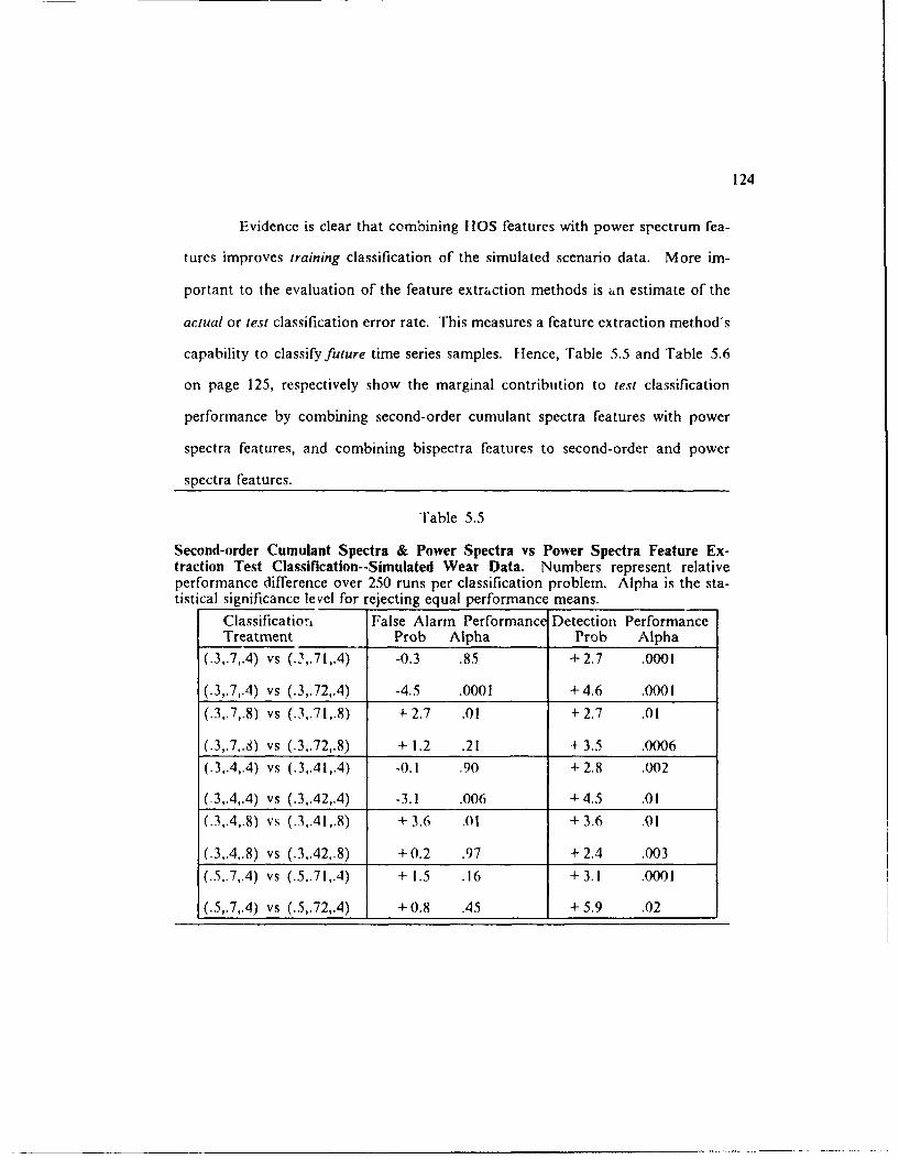
124

Evidence is clear that combining FIOS features with power spectrum fea-

tures improves training classification of the simulated scenario data. More im-

portant to the evaluation of the feature extraction methods is an estimate of the

actual or test classification error rate. This measures a feature extraction method's

capability to classify future time series samples. Hence, Table 5.5 and Table 5.6

on page 125, respectively show the marginal contribution to test classification

performance by combining second-order cumulant spectra features with power

spectra features, and combining bispectra features to second-order and power

spectra features.

Table 5.5

Second-order Cumulant Spectra & Power Spectra vs Power Spectra Feature Ex-traction Test Classification--Simulated Wear Data. Numbers represent relativeperformance difference over 250 runs per classification problem. Alpha is the sta-tistical significance level for rejecting equal performance means.

Classificatio:, False Alarm Performance Detection PerformanceTreatment Prob Alpha Prob Alpha

(.3,.7,.4) vs (.,.71,.4) -0.3 .85 +2.7 .0001

(.3,7,4) vs (.3,.72,.4) -4.5 .0001 +4.6 .0001

(.3,.7,8) vs (.3,.71,.8) +2.7 .01 +2.7 .01

(.3,.7..S) vs (.3,.72,.8) + 1.2 .21 +3.5 .0006(.3,.4,.4) vs (.3,.41,4) -0.1 .90 +2.8 .002

(.3,.4,.4) vs (.3,.42,4) -3.1 .006 +4.5 .01

(.3,.4,.8) vs (.3,41,8) + 3.6 .01 + 3.6 .01

(.3,.4,8) vs (.3,42,8) +0.2 .97 +2.4 .003(.5,.7,.4) vs (.5,.71,.4) + 1.5 .16 +3.1 .0001

(.5,.7,.4) vs (.5,.72,.4) +0.8 .45 +5.9 .02

125

Table 5.6

Bispectra, Second-order Cumulant Spectra, & Power Spectra vs Power Spectra Fea-ture Extraction Test Classification--Simulated Wear Data. Numbers represent rel-ative performance difference over 250 runs per classification problem. Alpha is thestatistical significance level for rejecting equal performance means.

Classification False Alarm Performance Detection PerformanceTreatment Prob Alpha Prob Alpha

(.3,.7,.4) vs (.3,.71,.4) -1.0 .45 + 3.4 .0001

(.3,.7,.4) vs (.3,.72,.4) -4.9 .0001 +6.8 .0001

(.3,.7..8) vs (.3,.71,.8) -0.2 .88 +0.3 .81

(.3..7,.8) vs (.3,.72,.8) + 1.2 .30 +3.9 .001

(.3,.4,.4) vs (.3,.41,.4) -1.5 .32 + 1.8 .002

(.3,.4,.4) vs (.3,.42,.4) -6.5 .0001 +6.2 .002

(.3,.4,.8) vs (.3,.41,.8) + 3.0 .005 + 3.0 .005

(.3,.4,.8) vs (.3,.42,.8) +0.07 .01 + 1.0 .0009(.5,.7,.4) vs (.5,.71,.4) -0.4 .73 +4.6 .0001

(.5,.7,.4) vs (.5,.72,.4) -0.5 .69 +7.0 .004

When the feature information set includes both stationary (power spec-

trum) and nonstationary (second-order cumulant spectrum) components, better

test classification performance is obtained. Significantly, detection performance

is increased for all treatments. Additionally, within each pair of treatments, or

scenario, a greater change in the phase modulation index parameter is accompa-

nied with an increased false alarm and detection capability. Thus, IIOS features

appear sensitive to greater changes in phase modulation which implies they have

an increasing ability to detect more severe wear condition states. Noise does im-

pact classification performance, but the IIOS approach still maintains its superi-

ority over the power spectrum approach. Combining nonlinear (bispectrum)

feature information further improves test classification performance. Thus, there

126

is an increasing marginal benefit for conducting IIOS estimation for subsequent

feature extraction.

5.3 Actual Wear Experiment Description

Electronic circuit card construction begins with sandwiched layers of very

thin copper and epoxy-glass composite material. Holes are drilled through these

layers to provide pathways for interconnections between the copper conductor

layers and sites for solder attachment of electronic components. A typical elec-

tronic panel consists of 1000 to 5000 holes with diameters of .5 mm to 2.5 mm.

ligh-speed machines (20,000 to 200,000 RPM) can drill I to 5 holes per second

with either single or multiple drill spindles. The drilling machine used by IBM in

their experimental study has a drilling capability of up to 75,000 RPM and is

shown in Figure 5.3 on page 127. Ramirez (1991) gives a complete description

of the mechanics of the machine structure.

Most circuit card manufacturing defects can be traced to problems in the

drilling process (Block, 1989). Problems caused partly by worn or damaged bits

include rough hole surfaces due to glass fiber tearing, smearing of epoxy from high

bit temperatures, and poor hole location and variation in hole diameter because

of drill wander. Thus, there are three major reasons for IBM and others in in-

dustry to investigate drill bit wear monitoring methods: (I) to improve the quality

of finished electronic panels by reducing incidence of poor quality holes; (2) to

reduce panel scrap costs by reducing incidence of badly damaged holes; and (3)

to reduce bit replacement costs by using as much of its useful life as possible.

Clearly, panel quality is a function of hole quality, which in turn, is a function of

127

Variable Speed Drive

Solenoid &Tubn&Canm Follower Thubiet

Bearing

Air Supply Baig

Panel Stack Fo

Clamp

X-Y Table

Figure 5.3: Drilling Machine used for IBM Wear Experiment

128

drill bit condition and engineers in this particular manufacturing application agree

that there is some point that hole quality degrades as drills wear, necessitating a

bit replacement strategy. Presently, drill bit replacement strategy is conservatively

based on the shortest observed useful life since there is no effective wear moni-

toring system implemented in the industrial environment. Actual wear varies with

lot-to-lot changes in the workpiece, drilling rate, condition of drilling machine, and

type of drill bit. Drill bits characteristically exhibit large variances in tool life.

IBM experiment instrumentation included X (lateral), Y (translational),

and Z (vertical) accelerometers, a magnetic reluctance probe, and X and Y

capacitance probes (see Figure 5.4 on page 129). This study focused on the

accelerometer signal data. Two accelerometers (X and Y) were bonded to the

journal bearing block to measure lateral acceleration transmitted from the drill

spindle to the machine structure. The Z accelerometer was mounted to the thrust

bearing block which moved with the spindle.

5.3.1 Experimental Design

A factorial experimental design with three factors was employed: age of

bit, material stack type, and chip load. Chip load is the amount of axial distance

travelled by the drill bit tip in a single revolution or rotation. There were two

levels for bit age (new or no holes drilled, and slightly used or 8000 holes drilled),

three levels of stack type ( NIP. 6S21', and short NIP), and two levels for chip load

(3 mil/revolution and 4 mil/revolution). A 1.09 mm diameter drill with a spindle

speed of 47,000 RPM and nominal chip load of .076 mil/revolution was used.

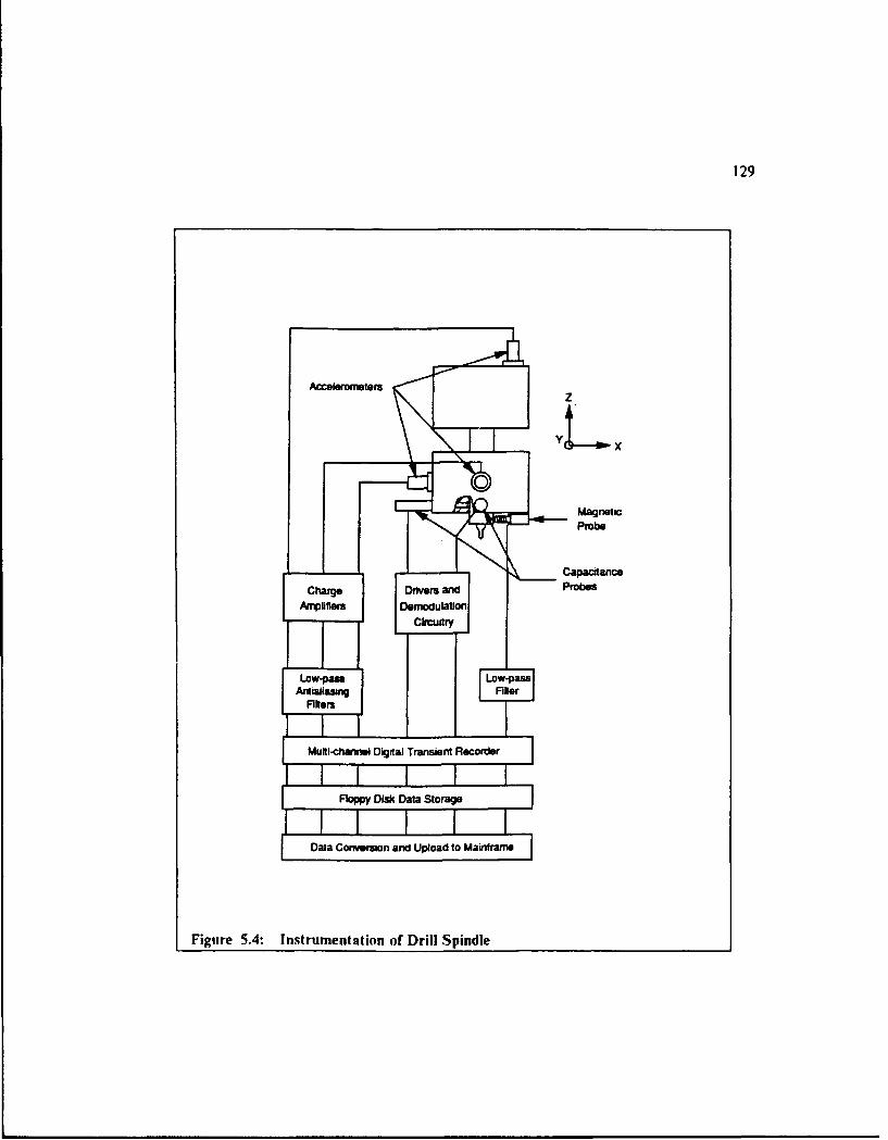
129

Accelerom~eters

MagneticProbe

Floppy DisCDatacStonae

Chaae Doao rivUpsoad orobesam

Figue 54: strmlfent mouation rl pnl

130

5.3.2 Collected Data

Vibration time series for each of the three accelerometers were analyzed

for two types of drill bits, new and slightly used. Ten bits of each type were ran-

domly selected and optically verified for wear condition. Figure 5.5 contains

magnified pictures of a typical new and slightly used drill bit. New and slightly

used bit data were obtained for both chip loads and two of the three stack types.

Shown at Figure 5.6 on page 132 and Figure 5.7 on page 133 are raw

accelerometer time series for a typical new and slightly used drill bit for one of the

stack material/chip load cases. There were three replications, or runs, for all

eighty bits in the experimental database which produced 720 time series records.

Preliminary estimation, feature extraction, and classification analyses consistently

showed the best sensor site for bit class discrimination was the vertical or Z

accelerometer. This conclusion was confirmed in a physical sense as the thrust

forces are additive rather than subtractive, and had bettet signal-noise character-

istics than either the X or Y accelerometers. Thus, results presented in this report

are only for the Z accelerometer. For computational purposes, each 3 mil/rev (4

mil/rev) time series is divided into appropriate record lengths as given the respec-

tive 760 liz (587 liz) harmonic frequency of the drill spindle, an integer number

of signal periods was necessary to avoid the effects of leakage when performing

spectral estimation procedures. Power spectrum, cumulant spectrum, and

bispectrum estimates are computed over blocks within each time series record.

All spectral estimates are averaged over appropriate block lengths, and then in-

corporated into the ensemble averaging of all samples of its particular class.

131

Figure 5.5: Magnified Photos of New and Slightly Used Drill Bit

132

sapl tim seie ofa nebefo h ceeomeer

-- L ....

U ------- --- -- ---- - .

- ' a.!

Figure 5.6: Raw Accelerometer Time Series--6S2P/4 Case (New Drill). Onesample time series of an ensemble from the Z accelerometer.

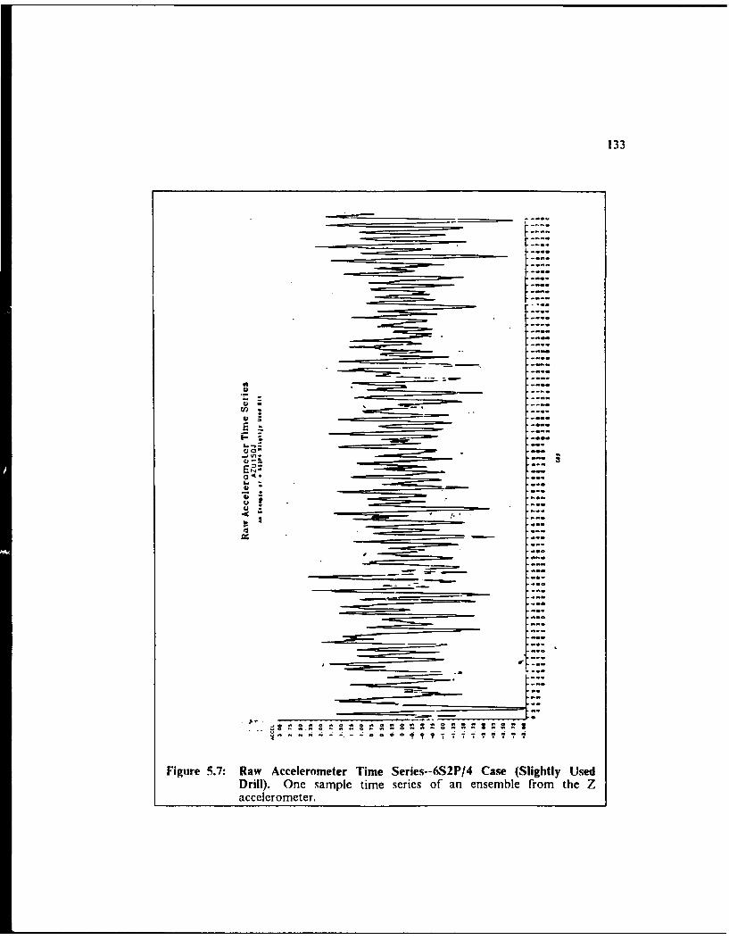
133

Ego

(-J o

d --'

Er9

GA - "a-

rr0Z

aaa~a

Figure 5.7: Raw Accelerometer Time Series--6S2P/4 Case (Slightly UsedDrill). One sample time series of an ensemble from the Zaccelerometer.

134

5.3.3 Results

Performance results are given as two separate but related categories, dis-

crimination and classification. Both performance categories are reported by indi-

vidual stack material and chip load case, combined chip load, combined stack

material, and corresponding averaged values. Performance results obtained for

combined data address the impact of drilling process parameter variation such as

stack type and cutting conditions on the feature extraction methodology. It is

desirable from a monitoring system implementation perspective that the feature

extraction and classification methodology should not be severely impacted by

process parameter variation. There are various statistical measures to compare

the discriminating power of the feature extraction methods. In this study, the ap-

proach is to first report Wilks' lambda and squared canonical correlation measures

for the training or discriminant rules constructed from the number of existing

samples in the experimental database for the data partition types. However, since

classification is the major objective in many applications of discriminant analysis,

alternative spectrum feature extraction approaches are also compared by examin-

ing two major classification performance components which define the rate of

correct classification: probability of detection and probability of false alarm.

5.3.3. I Discrimination

Shown in Table 5.7 on page 136 is the marginal benefit of combining

I IOS feature sets with power spectrum features for discrimination effectiveness.

Both the Wilks' lambda statistical criterion (smaller is better) and the averaged

135

square canonical correlation measures had significant margir1 *,-,provement in

six of the eight partition database types. For the two cases ofno overall marginal

improvement, NIP4 and NIP, differences are not significantly different from a full

I IOS feature approach (spectrum, cumulant spectrum, and bispectrum) versus just

power spectrum features. Recall from Chapter 4 that the most significant

second-order cumulant feature for the NIP4 case was on, rather than off, the

2-CSPD diagonal spectral support line. Significant marginal improvement for the

other six cases is obtained by combining cumulant spectrum (nonstationary) fea-

tures to power spectrum (stationary) features, and for combining bispectrum

(nonlinear) to stationary and nonstationary feature sets. Additionally, marginal

improvement is gained by combining nonlinear feature information for all data-

base partitions, and particularly for the two cases of no overall marginal im-

provement between IIOS and power spectrum feature extraction discrimination

effectiveness, a large marginal improvement with nonlinear features was gained.

136

Table 5.7

Marginal Discrimination Benefit of HOS Features versus Only Power SpectrumFeatures--Actual Wear Data. Both effectiveness measures represent relative dis-criminating power of a specific discriminating function computed on thirty vi-bration time series of each bit class, new and slightly used. Power spectrum isdenoted by 'PS', second-order cumulant spectrum is denoted by '2C', andbispectrum is denoted by 'B'.

Discrimination Wilks' Lambda Squared Canonical CorrCase PS PS&2C PS,2C&B PS PS&2C PS,2C&B

NIP/3 .429 .561 .295 .570 .438 .704

NIP/4 .379 .462 .430 .620 .537 .569

6S2P/3 .510 .370 .299 .489 .629 .700

6S2P/4 .555 .530 .392 .444 .470 .607

Stack/Load Average .469 .480 .354 .530 .518 .645

Chip Load 3 .609 .600 .530 .390 .399 .469

Chip Load 4 .736 .525 .353 .263 .474 .646

Load Average .673 .562 .441 .327 .437 .558

Nil Stack .399 .656 .456 .600 .343 .543

6S21) Stack .684 .536 .446 .315 .463 .553

Stack Average .541 .596 .451 .458 .403 .548

Inspection of the I1OS discriminant functions constructed for each data-

base partition type using stepwise discriminant procedures revealed the more sta-

tistically significant and number of variables were of the I IOS variety rather than

the power spectrum. Although not shown in Table 5.7, results (lid show From the

standpoint of discriminating power, one type of spectrum Fature extraction vector

by itself (power spcctrum, bispectrum, or second-order cumulant spectrum) is not

137

as powerful as the combination of feature types. In summary, 1lOS estimation

and feature extraction methods provide a substantial improvement in these two

discriminating effectiveness measures for the drill bit wear data and appears useful.

5.3.3.2 Classification

Combining IlOS features to power spectrum features clearly improves

discrimination power. Equally important to an evaluation of the feature ex-

traction methods is an estimate of the expected actual classification error rate.

Results are given with tables identified by the applied multivariate classification

algorithm, two parametric approaches (linear and quadratic discriminant or LDF

and QDV) and one non-parametric approach (k-nearest neighbor). Results are

stated in the following manner: (1) within a classification algorithm, a direct

one-to-one comparison of the feature extraction methods for stack/load and also

for the combined process parameters (cutting condition and stack material) clas-

sification cases: and (2) a comparison of feature extraction method performance

across classification algorithms for all classification cases. Comparison of the

feature extraction methods in this fashion allows an evaluation of each approach

for its sensitivity to stochastic process conditions and also to the classification al-

gorith m.

The contribution of combiting I IOS features to power spectrum features

using a linear classifier is shown in Table 5.8 on page 13q. LI)F classification

results demonstrate the marginal benefit of performing IIOS estimation and fea-

ture extraction for all classification cases. Averaged classification performance

measures (stack/load, load, and stack) reveal combining I IOS features with power

138

spectrum features obtains an increasing marginal benefit in terms of overall clas-

sification accuracy. False alarm rates may be higher in some cases, but the mar-

ginal increase in detection capability makes up for the difference in lost capability.

This performance result is significant as a higher detection capability is more de-

sirable than a lower false alarm rate in most industrial manufacturing situations.

For each of the feature extraction approaches, better performance is obtained with

databases which are the most homogeneous. Also, they all have better classifica-

tion ability with the combined stack material database than the combined cutting

(load) database. Thus, there is less sensitivity to cutting (chip load) variation than

stack material variation which agrees with a major finding of Ramirez (1991) that

variations in circuit card construction can mask the effects of wear. Significantly

though with the more heterogeneous data (combined load and combined stack),

the performance of the FIOS approaches is not degraded as much as the purely

power spectrum approach.

139

Table 5.8

HOS Feature Extraction versus Solely Power Spectrum Feature Extraction Classi-fication Using LDF Algorithm--Actual Wear Data. Numbers represent percent ofthirty slightly used drill bits incorrectly classified as new, or false alarm rate, andpercent of thirty drill bits correctly classified as slightly used, or detection rate.Power spectrum is denoted by 'PS', second-order cumulant spectrum is denoted by'2C', and bispectrum is denoted by 'B'.

Classification False Alarm Probability Detection ProbabilityCase PS PS&2C PS,2C&B PS PS&2C PS,2C&B

NIP/3 .133 .366 .200 .850 .966 .933

NIP/4 .133 .250 .233 .933 1.00 .966

6S2P/3 .150 .166 .100 .862 .933 .896

6S2P/4 .283 .350 .150 .816 .933 .916

Stack/load Average .175 .283 .170 .865 .958 .927

Chip Load 3 .150 .316 .300 .728 .850 .816

Chip Load 4 .258 .300 .233 .675 .866 .850

Load Average .204 .308 .266 .701 .858 .833

6S2P Stack .250 .316 .200 .661 .950 .933

NIP Stack .183 .333 .250 .933 1.00 .900

Stack Average .216 .324 .225 .797 .975 .917

Shown in Table 5.9 on page 140 is the marginal contribution of combin-

ing I IOS features to power spectrum features using a quadratic classifier. Similar

marginal benefit results with IIOS information are obtained as with a linear

classifier, but the more difficult parametric classification, quadratic rather than a

linear function, is not beneficial for the power spectrum feature extraction ap-

proach.

140

Table 5.9

HOS Feature Extraction versus Solely Power Spectrum Feature Extraction Classi-fication Using QDF Algorithm--Actual Wear Data. Numbers represent percent ofthirty slightly used drill bits incorrectly classified as new, or false alarm rate, andpercent of thirty drill bits correctly classified as slightly used, or detection rate.Power spectrum is denoted by 'PS', second-order cumulant spectrum is denoted by'2C', and bispectrum is denoted by 'B'.

Classification False Alarm Probability Detection ProbabilityCase PS PS&2C PS,2C&B PS PS&2C PS,2C&B

NIP/3 .183 .366 .333 .833 1.00 1.00

NIP/4 .183 .166 .2t, o .833 .966 .966

652P/3 .150 .200 .100 .810 .966 .931

6S2P/4 .300 .300 .250 .700 .816 .883

Stack/Load Average 200 .258 .220 .794 .937 .945

Chip Load 3 .175 .366 .266 .737 .916 .950

Chip Load 4 .258 .266 .116 .675 .833 .900

Load Average .216 .316 .191 .706 .874 .925

6S2P Stack .241 .266 .133 .635 .933 .933

NIP Stack .108 .400 .333 .933 1.00 1.00

Stack Average .175 .333 .233 .784 .967 .967

Average stack/load classification is degraded with power spectrum features and

has no consequential impact on either averaged load or stack classification.

I lowever, the impact on averaged total classification accuracy using I IOS features

is: -1.5 percent for stack/load, + 8.3 percent for combined load, and + 2. I percent

for combined stack. For the stack/load case, false alarm rate increased more than

the corresponding increase in detection capability so there was a slight decrease

141

in overall QDF classification performance for this database partition. However,

the masking of wear effects due to variations in card construction is not as great

with HOS features and QDF classification. The major disadvantage of a power

spectrum approach is almost overcome. Significantly, detection capability was the

major component of the increase in the LDF classification accuracy of HIOS fea-

tures using a QDF approach.

The marginal contribution of combining HOS features to power spectrum

features with a non-parametric classifier (k-nearest neighbor with k= 4) is shown

in Table 5.10 on page 142. Direct comparisons of these classification results

clearly show the increased overall classification power of the IIOS feature ex-

traction approach. There are increases in both false alarm and detection capabil-

ity with IlOS features. Additionally, increasingly marginal benefits are evident as

more spectral feature types are combined. Nearest neighbor classification makes

no difference or degrades previous parametric classification results with solely

power spectrum features due to increases in false alarm probabilities. lowever,

the amount of increased total classification accuracy due to the non-parametric

method ranges, in an absolute sense, from 3 to 8 percent, with combined fIOS and

power spectrum feature sets. Additionally, combined chip load classification with

power spectrum and cumulant spectrum features is only slightly degraded with the

change in card material. There is no doubt non-parametric classification

(4-nearest neighbors) is the best classification approach with this incipient drill

wear database.

142

Table 5.10

HOS Feature Extraction versus Solely Power Spectrum Feature Extraction Classi-fication Using 4-Nearest Neighbor Algorithm--Actual Wear Data. Numbers repre-sent percent of thirty slightly used drill bits incorrectly classified as new, or falsealarm rate, and percent of thirty drill bits correctly classified as slightly used, ordetection rate. Power spectrum is denoted by 'PS', second-order cumulant spec-trum is denoted by '2C', and bispectrum is denoted by 'B'.

Classification False Alarm Probability Detection ProbabilityCase PS PS&2C PS,2C&B PS PS&2C PS,2C&B

NIP/3 .150 .266 .133 .850 .936 .983

NIP/4 .100 .166 .133 .933 1.00 .966

6S2P/3 .366 .300 .133 .844 1.00 1.00

6S2P/4 .183 .216 .200 .850 .933 .966

Stack/Load Average .200 .230 .150 .869 .966 .962

Chip Load 3 .4o8 .183 .316 .822 .933 .933

Chip Load 4 .175 .266 .200 .775 .933 .950

Load Average .291 .224 .258 .798 .933 .941

6S2P Stack .516 .183 .166 .745 .Q66 .983

NIP Stack .266 .233 .250 .900 .866 .933

Stack Average .391 .208 .208 .822 .916 .958

Usefulness of combining I IOS feature sets with power spectrum feature

sets is clearly demonstrated with the results gathered from simulated and actual

wear experiments. A [JOS approach for incipient fault detection has increased

discrimination and classification power and is less sensitive to process and noise

conditions than solely a power spectrum approach. Conclusions of the study are

stated in the next chapter.

Chapter 6

Conclusions and Further Research

Inferences from the data analyses of the conducted experiments are stated

in general and specific form. This research focused on cyclostationary processes

represented by simulations of single-tone amplitude and phase modulated carrier

signals which primarily emphasized phase modulation changes and new and

slightly worn high-speed drills in the "manufacturing environment". The evidence

clearly advocates for the adoption of a IIOS feature fusion approach in a condi-

tion monitoring scheme for rotating systems. Whether the HOS approach can

create actual economic savings in an industrial setting is a question left for further

research.

Two important general conclusions are drawn from the results of this

study:

I. Incipient fault detection capability of multivariate classifiers significantly im-

prove with I IOS feature information.

2. Better operations and maintenance decisions to discontinue/service rotating

systems are possible if the condition monitoring method incorporates the

I IOS feature fusion approach.

Five secondary research questions supported these general conclusions:

(I) What is the impact of combining I IOS features with power spectrum features

upon discrimination and classification of incipient Faults? (2) What is the impact

of a changing process environment upon classification? (3) What is the impact

of applied classifier algorithm upon classification? (4) What is the impact of a

143

144

slight change in phase modulation upon discrimination and classification? (5)

What is the impact of increasing noise in the signal environment upon discrimi-

nation and classification? Results from the modulated signal simulations an-

swered all secondary research questions except for the third one while results from

the actual experiment answered the first three questions.

In the simulation experiments, when the feature information set included

I-lOS features better discrimination power was obtained (see Table 5.2 on page

121 and Table 5.3 on page 122). Additionally, when the feature information set

included both power spectrum and second-order cumulant spectrum features,

better training and test classification performance was obtained than with just a

ower spectrum feature set (see Table 5.4 on page 123 and Table 5.5 on page

,L 4 ). Further improvement in training and test classification performance was

obtained when bispectrum features were combined with second-order cumulant

and power spectrum features (see Table 5.4 on page 123 and Table 5.6 on page

125). Thus, IIOS estimation for subsequent feature extraction provided an in-

creasing marginal benefit for a linear classifier. I lOS features were sensitive to

very slight changes in phase modulation which implied the ability to detect incip-

ient faults and a greater potential capability to detect more severe wear condition

states of rotating machinery. Finally, noise impacted classification performance

whether with or without I IOS information. I lowever, with moderate or even high

levels of noise in the signal environment, IIOS approaches were still better at de-

tccting different simulated signal classes with very high levels of statistical confi-

dence (see 'rable 5.5 on page 124 and Table 5.6 on page 125).

In the actual experiment, when the feature information set included power

spectrum and second-order cumulant spectrum features, better discrimination

145

power was obtained than a feature set based only on the power spectrum. Further

discriminatory power was obtained by combining bispectrum features with

cumulant spectrum and power spectrum feature sets (see Table 5.7 on page 136).

This same marginal beneficial trend was demonstrated with classification results.

When power spectrum and second-order cumulant spectrum features were com-

bined, classification performance increased from that of a power spectrum feature

set. The classification performance further improved for all three applied

multivariate classifiers when bispectrum features were combined with cumulant

spectrum and power spectrum feature sets (see Table 5.8 on page 139, Table 5.9

on page 140, and Table 5.10 on page 142).

Actual wear classification results presented in the tables of Chapter 5 are

now condensed as total classification averages (see Table 6.1 on page 146). All

feature extraction methods were sensitive to changes in process parameters.

Ilowever, IIOS feature extraction was less sensitive than solely power spectrum

feature extraction. Specifically, variations in card construction significantly

masked the effects of wear when power spectrum features were used for all clas-

sification approaches. Also, chip load variation masked the effects of wear when

power spectrum features were used with two of the three classifiers. However,

variations in card construction and chip load only slightly masked the effects of

wear when power spectrum and cumulant spectrum features were used with the

4-nearest neighbor classifier. Furthermore, variations in card construction and

chip load had no wear masking effect when full IOS feature sets were used with

a quadratic classifier. By selecting and combining I-OS features which captured

the nonstationary and nonlinear characteristics of the cutting forces as the drill

146

bit penetrates the circuit card layers, total classification capability was definitely

enhanced.

Table 6.1

Actual Incipient Wear Total Classification Averages. Combined load databasetested the impact of stack variation, combined stack tested the impact of load var-iation, and load/stack was the most homogeneous database partition with no vari-ation of drilling process parameters. 'PS' represents power spectrum, '2C'represents second-order cumulant spectrum, and 'B' represents bispectrum. 'LDF'and 'QDF' denotes linear and quadratic parametric classification, and 'NN' denotesthe nearest neighbor non-parametric classification.

Features and Combined DataBases Homogeneous DataBaseClassifi,'ation Comb Load Comb Stack Load and Stack

PS & LDF 75.1 79.1 84.5

PS, 2C & LDF 77.9 82.6 83.8

PS, 2C, B & LDF 78.3 84.6 87.8

PS & QDF 74.5 80.5 79.7

PS, 2C & QDF 77.9 81.7 84.0

PS, 2C, B & QDF 86.7 86.7 86.3

PS & NN 75.4 71.6 83.5

PS, 2C & NN 85.4 85.4 86.8

PS, 2C, B & NN 84.1 87.5 90.6

Thus, results of all five secondary research questions revealed that a con-

dition monitoring approach based on power spectrum characteristics was more

sensitive to external noise and stochastic process parameter variation than that

which incorporated tIOS information. These results provided statistical evidence

for the two general conclusions of the study and clearly demonstrated the benefits

147

of IIOS estimation and feature extraction as preprocessing steps for a multivariate

classifier.

6.1 Areas of Further Research

Further studies are possible in both the applications and methodology

areas. First, analysis of IBM extended drill wear data, already gathered and ob-

tained, is needed so more than two classes of drills can be examined. I lence,

testing the ability of classifiers with and without HOS features to detect different

levels of drill wear can be investigated. The particular HOS feature sets selected

from analyses of the incipient wear factorial experiment can be further examined

for their predictive ability of advancing drill wear. It is already known that the

fifth through the eighth harmonics of the Z acceleration power spectrum were

most sensitive to advanced drill wear (Ramirez,1991). These particular power

spectrum responses steadily increased as drill wear progressed, and rapidly in-

creased when drill wear-out was achieved. Quite significantly, the bispectrum

chloropleth difference plots of each case of the incipient wear data revealed these

same harmonic frequencies interacting with higher frequencies to be among the

most significantly different frequency interactions between classes! It is possible

that bispectrum analysis can be used as a predictive tool of advancing wear.

Second, a large database of pump and fan failure data obtained from TRACOR

(Austin) can be studied for applicability to other rotating machinery besides

high-speed drills. The TRACOR data is already analyzed by some of the vibration

analysis techniques mentioned in Chapter 2. Results from the I IOS analytical

approach could be compared with the results of these other techniques. Third,

148

other classification algorithms such as neural networks could be applied to inves-

tigate whether trends identified in this research continue to hold. Obtaining the

right type of information required for proper further investigation of the IIOS

approach is tedious, difficult, and expensive. The hard work of obtaining excel-

lent experimental data is done as both rotating machine failure databases are

available from the author. Some ideas of expanding on the methodological work

is given next.

First, third-order cumulant estimation and feature extraction can be per-

formed for the experiments described in this work. This is extremely important

to investigate as the contribution from this cumulant spectrum measure will

probably be more significant than the second-order cumulant. Second, more in-

volved and complicated simulation experiments such as testing with differing lev-

els of the experimental parameters and also multiple-tone simulations are needed.

Third, more investigation with regard to the correspondence of the statistical

findings of this research to the actual physics of wear processes occurring in

high-speed drilling of composite circuit card materials is a good research project

for a mechanical systems graduate student. Finally, depiction of how the statis-

tically significant features change and move through spectral principal domain

regions ovcr multiple conditions of the machine is another area for methodological

resea i ch.

6.2 Summary

This research study was significant in many respects. This is the first

work to provide a rigorous study of the IIOS approach in detecting incipient

149

faults. Moreover, this is the first work to address the nonstationary aspects of

random fault mechanisms. Most incipient fault detection methods are usually

tested against one specific application or machine system. Due to the inherent

stochastic nature of the systems under study, a statistical and experimental design

framework is necessary to thoroughly investigate a particular monitoring ap-

proach. Deriving statistical conclusions which show consistency with both simu-

lated and actual time series signals gives validity for the new [JOS monitoring

approach. Understanding the necessity to investigate and justify structural as-

sumptions such as linearity, Gaussianity, and stationarity of time series data is one

of the major lessons learned in this study. This research explains the procedures

for manipulating such time series data so that other rotating machinery situations

can be properly analyzed. Because the research approach provides the tools for

investigating and exploiting a wider potential range of time series characteristics

generated by random fault mechanisms of cyclostationary processes, improved

exccutive decisions in both the maintenance and operational environments of ro-

tating machinery are possible.

A ppend ices

AppenG'X A

Second-Order Cumulant Spectrum Estimation Program

152

W ofp4~ila

666 II. ... l s.I Me as1 .4"IS .04 lt '

Got To* do"

.11 W

1#1 .174 j t 7 'i: m

K im :t*557 ade1M7 NT621

u - e 11 m :7 1 *

U ISAI

HPi, .00*1

11 1 : * II .C~

LO*iI

153

I I~L

* at..Iat. to. .. w at bI..ft.. d-f.d -tat*

A, I- t. 4.1

CACCU1W T IEST 2TATIIlt FORMOaMis

SISSLAItlK Uh*tI

* .i .. fn. -9C k.- Li.st. Tob).ad

'r C 41 Md" Far If"b M. P *ased.

I ftt.4l.0 *fill

goa eAAtflUsb

IFIC*Ci.;.I~qgLPIAC KNIMIIJLA Out,~2~* .Cgql

4, rT; of UftsC CSiLN'*T tIVIS~ZAC ICEAK

ve 111 .: **i P: I

C.A C C.,l.A. *n, It. t..

gul Uf,: -tiff ..

PSA I.. o ON AIO lAP INPT DTA ILI

To.Tn.* fit.~ @..e . IA.:V..

t? UCA r" PC.F.... . A. 'atUVR . ."~.t.L , l

.1.. rlt *n1f I. p.

*A Ait, cAO. * P. SA.SC

154

* -slw* Use, tim rigza- 's,

do ,41 *949.f.M

* .p.. 1. 1. .. d

lot e AUB - s free.

Al9PP L. :2? ,..9..6

LAVA, 4. t . tt

INU *1'99 *blllf...3 b~~~t~ .s.S9£9t

me00ie A3£.I ItEA t .- twa ~ ~ ~ ~ ~ IBI I0pq ..4". .zua i ,

UAL C at13.4..

041~.99 Pt"I"M

Is.TP. ~ 1 .18 1 18.2 39-d

19943£Tt ~ ~ :4 1.,-,CLSF

LE.S LPSICCSJ9T

-dSOMP9Ol17( 199£9133.~.9.,IISVS.U

.999£.1.W. l .-. 9.9.. 1 PV 9A i.9.9.9..

C L.S99£99rl.dPW.4.V£.~1i.. *f9.££'.LL99.9C

HIM,-~ 9.CC£9en*

155

,:'d*sama:3 r-..au

-a'". d

So@30.4

ecits lst.a

=iI E'fi. S..M. .P f.J w o1

M. topi 05 0.ai -W 1"I.

goi5. t . fl-t**tS. 4 taS

I a I M1aa1a to

Ktos bt. d

-.- 'aMI*4t" " 1.7:

.~a- smt... O~j0B-I.to .,Pa~rVBS.t a .aiI

00of "Mo Is5 ..aiIs ts,.

156

I% PrRACTNLes :z "ev" 11111.

ff... ii ... t

ims. f 1fb * ~ *

a-4

* 1 PI bi. *... *i -tit..

bl qolo,"ou. -..

157

wooal *auR.e 4

asw I. --

ITI

w .M. . stL

As, al: *r.. is ot r

11C '511 fe~S~

IC? 1'9 1.. 1 UeSIt

IM

C I ACC.C. ffC..: r. FU: *P-iea M~R~R~

4 RSAR~UWu lawm'm it h' ia 1I,

Ca aC pc-eC~we :Wqw TO-it a~)C awL&"Eza IC.a

C CRC SAt

C ev C SCRCW,* igb 31 STR 31£ NCs" ails.

A: CR57 r S f '00, a valm O' WIM IsK m

C ~ ~ ~ ~ ~ ~ ~ i at-*Cew SS in tw,

C CCIICCA. n A t.C F.* ~ ~ ~ ~ o CC )CCS-Cm33CRmervPIU

* ~ ~ f I RC IRUSC.C

IRCCC.CC * ZI.C , I

158

Isai W.1beem4to.~wil

m..i~f.

ROMdo~i~I. OV

an 1 A.

in a -1 so to Ino~u

11?

use

1.dLM:OCSCCM1I

11 l-31a

do

i f. ft. j IP8 t

4* 11 .. 0

159

rt...

.09 toI a y 1

13:

SI.. -1 ... I ...

" i~ Ii., •a*aIh.3..11E1

lit 61 L o -II.

j4i.14 l i 4.:g

lerw~

.llt.."it I~i!-tl tAs,1; .,,....,f.. -.91."

do11 , -.I

11e 1* -.. ..44 .,.9 _.!.i..

.9..1.949.I RV IMIri.

Mlli'|"tl~l

160

FL

umu

:1PA)-. t

C"31

* Sle I ufl - I

a .ll*

____ jji III lf *,tJl J. SS *ftll...

111,13:11" :

II1b1 i* •.3 ** I*!

, 1 . al~.5 .H-,

II'...."Ii ..tol = =~ ~IeSt ,,,e

I • ..I .1-,.si

I :.: 4 ;~ii, t "

.aS•. • . C~uJzi i **

1,

4II I 39 I-

Appendix B

Harmonic Process Model Stationarity and Finite Memory

162

Harmonic Process Model (HPM) Stationarity and Finite Memory

When b, are independent uniformly distibruted random variables, V(t) is

always stationary irrespective of A. and a), values. There are two conditions for

stationarity:

E[V]= 0 for all t [B- 1]

and

CoV(V 1 , V2) = CoV(r) = n (T) [B - 2]

where r is the time shift or lag parameter.

B-I is easily shown first and consirler B-2 for the n= I case. The argu-

ment shown is easily extended to the general case. Because of the given informa-

tion the expected value of V (t) is:

,T V(t)] = a cos(wA, t + O)d~k

. 2a- [ sin(wlt) 4 = 0 for all t

Now for the second condition for stationarity.

163

Cov(V1,V2)=E{V(t)}{V(t +) r=O,±-I,+2....

a0 2 JOO

a2 00_a - cos(wt + 4b) cos(o,(t + r) + 4')do

4na [ cos ((2ot + oT) + 2} + cos COz]dba (cos ,,,)do4, = a c ]

2

_ a -[7 CO - ( - T) cos " ]47r

2 2a (2aos- (2.r COS Gr) a CUS(Wt).

For the general case

o24

li!R(T a.n= 0COSwflT

n=O

Thus, the autocorrelation fiction p(r):

2Za, COS (s),T

R(r)_

R(O) Z=02= ~0)n

n=O

164

So, both the autocorrelation and autocovariance functions of a harmonic process

consist of a sum of cosine terms and thus never die out. This is in contrast to

MA and A R processes and so the finite dependence assumption, or finite memory,

is not applicable for IIPM. Stationarity is applicable no matter what choice is

made of the amplitude and frequency terms.

Appendix C

Power Spectrum Broadening

166

Cosine-Wave Carrier Signal Spectrum Broadening

Signals generated from rotating machinery not yet performing a particular

machining process produce a pure harmonic tone due to its periodic driving force

mechanism: cos 2nft = cos coj. However, once machining is performed, the gen-

erated signal is:

Vampm(t) = k[I + mai(t)] cos(ot + 0, + mg(t)) + n(t)

Notation described in the report text is repeated in this appendix but is condensed

for ease of presentation. In the text, Vo,,,(t) is the amplitude and phase modu-

lated cosine-wave carrier signal, m. is the amplitude modulation index, fit) is the

amplitude modulating signal, 0, is the carrier signal phase, m, is the phase modu-

lation index, and g(t) is the phase modulating signal. Now,

fit) = cos wot and g(t) = cos w),t with f, andf, are the frequency of the amplitude

and phase modulating wave, respectively. Briefer notation for this appendix is the

following:

Vamp(t) = k[! + m(t)] cos(wct ± 0(t) ± 0)

whz- andoin amplitude and phase modulations are represented by re(t) and 4(1)

respectively. and 0 is the random carrier phase variable that is independent of both

the random amplitude and phase modulation variables and has the same uniform

pdf. If m(t) and (I) are zero mean, stationary, and statistically independent ran-

dom variables, the power spectral density of I',,(t) is now derived.

First, the autocovariance (R,-- [V(t) V(i') ]) is computed:

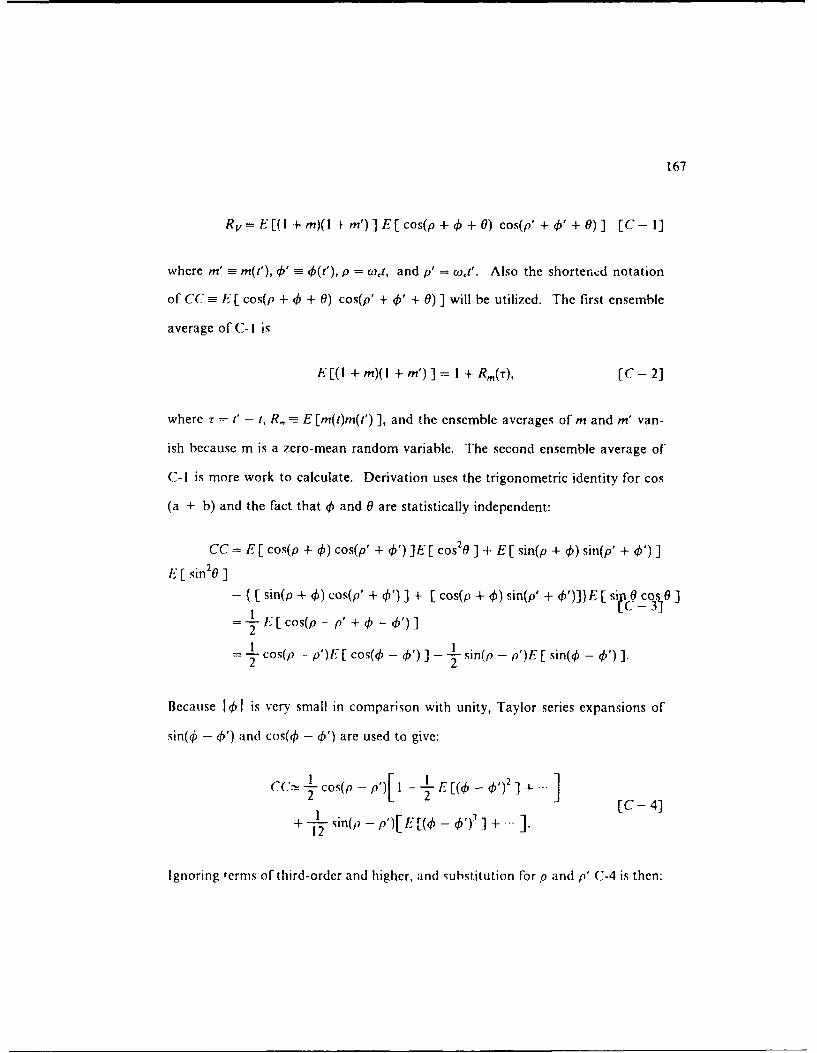
167

Rv= E[( I +m)(I +m')]E[cos(p+4) +0) cos(p' +4' +0)] [C- I]

where m' = m(t'), 0' =4_(t'), p = cojt, and p' = cot'. Also the shortened notation

of CC = E [ cos(p + 4+ 0) cos(p' + 0' + 0)] will be utilized. The first ensemble

average of C- I is

E[(l + m)(I + m')] = I + R,.(t), [C- 2]

where T = t' - t, R,= E [m(t)m(t') ], and the ensemble averages of m and m' van-

ish because m is a zero-mean random variable. The second ensemble average of

C-I is more work to calculate. Derivation uses the trigonometric identity for cos

(a + b) and the fact that dh and 0 are statistically independent:

CC = E [ cos(p + 0) cos(p' + &) ]E [ cos20 ] + E [ sin(p + 0) sin(p' + h')]

E[ sin20 ]

- { [sin(p + 'k) cos(p' + ')] + [ cos(p + 40) sin(p' + 0')]}E [ si 0 cos0]

E [ cos(p - p' + -

3

2

- cos(p - p')E [ cos(4 - h') - sin(p - p')E [ sin(4, - 4')].

Because 1 is very small in comparison with unity, Taylor series expansions of

sin(4 - 4,') and cos(O - 4') are used to give:

2 2 [C - 4]+ -L2 sin(jp - p')[ E[(0 - 0') ] +

Ignoring terms of third-order and higher, and substitution for p and p' C-4 is then:

168

1CC = -- cos(C.:) [I - R0(O) + RO(r)]. [C - 5]

Finally, substitution of C-4 and C-2 into C-1 yields:

I

RJ() - -L [ I + Rm(T)][ I - R(O) + R(T)] cos Gj[C - 6]

- - [ I - R0(0) + R.(r) + R(T) cos o)cr,-2

where terms proportional to R,,R, are ignored due to their higher order in the

smaller quantities m and &.

The power spectral density is obtained by using C-6 in the standard defi-

nition of the power spectrum as shown:

P() = R()e

The result is:

169

P) 1 1(I a)fe-12 n(f-fj)Td

1 21 -i2 i(f +f )'4 0F

+ R a( e-I 2 ir(/-fc ) dr

4 -, [C- 7]

1 00 R(r)e-I 2 7r(f+f, r dT

4 f 00

1 R()e-i 2 ir(f- +f )r dr_00

Using the definitions of Dirac delta functions and the power spectrum C-7 be-

comes:

P(/) I r(I _ 2)[6(f-f) + S(ff)] +[C- 8]

I I P(f-f) + Pm(f+.fc) + Po(f-) + P v +f')4

where o = R,(O). From C-8 it is seen how the discrete spectral lines are broad-

ened by both amplitude, P), and phase modulations, P,.

171

"Computation and Interpretation of Kth Order Spectra." In SpectralAnalysis of Time Series, edited by B. Harris. New York: John Wiley, 1967b.

Brockett, P. L., Hinich, M. J. and Patterson, D. "Bispectral-Based Tests for theDetection of Gaussianity and Linearity in Time Series." Journal of theAmerican Statistical Association, Vol 83, No. 403 (1988), 657-664.

Brockett, P. L., Hinich, M. J. and Wilson, G. R. "Nonlinear and Non-GaussianOcean Noise." Journal of the Acoustical Society of America, 82 (1987),1386-1399.

Cramer, H. "On Some Classes of Nonstationary Stochastic Processes." . Pro-ceedings of the Fourth Berkeley Symposium on Statistics and Applied Proba-bility, 11 (1960), 57-78.

Dan, L. and Mathew, J. "Tool Wear and Failure Monitoring Techniques forTurning - A Review." International Journal of Machine Tools and Manu-facture, 30 (4) (1990), 179-189.

Darlow, M. S. and Badgley, R. 1i. "Applications for Early Detection of Rolling-Element Bearing Failures Using the I-igh-Frequency Resonance Tech-nique." ASME,, 75-DET-46.

Drago, R. J. "Incipient Failure Detection." Power Transmission Design, February(1979), 40.

Dyer, D. and Stewart, R. M. "Detection of Rolling Element Bearing Damage byStatistical Vibration Analysis." Trans. ASME, J. Mech. Design, 100 (2)(1978), 229-235.

Elbestawi, M., Marks, J. and Papazafiriou, A. "Process Monitoring in Milling byPattern Recognition." Mechanical Systems and Signal Processing. 3 (3)(1989), 305-315.

Fukunaga, K. and Ando, S. "The Optimum Nonlinear Features For a Scatter Cri-terion in Discriminant Analysis." IEEE Transactions on Information The-ory, IT-23 (1977), 453-459.

Gardner, W. A. and Franks, L.E. "Characterization of Cyclostationary RandomSignal Processes." IEEE Trans. Inform. Theory, IT-21 (1) (1975), 4-14.

Gardner, W. A. Introduction to Random Processes with Applications to Signals andSystems, New York: McGraw 1lill, 1989.

Ceorgel, B. Proceedings of International Signal Processing Workshop on hligher-Order Statistics, Chamrousse, France, July, 1991.

(ersch, W. "Two Applications of Parametric Times Series Modelling Methods."In Mechanical Signature Analyis, edited by S. Braun. London: AcademicPress, 1986.

172

Gladyshev, E. G. "Periodically Correlated Random Sequences." Soy. Math., 2(1961), 385-388.

Iland, D. J. Discrimination and Classification. New York: John Wiley, 1981.

Hasselman, K., Munk, W. and Macdonald G. "Bispectra of Ocean Waves." InTime Series Analysis, edited by M. Rosenblatt. New York: John Wiley,1963.

liclland, K., Lii, K. and Rosenblatt, M. "Bispectra and Energy Transfer in Grid-Generated Turbulence." In Developments in Statistics (Vol 2), edited by P.Krishnaiah. New York: Academic Press, 1979.

Hills, M. "Allocation Rules and their Error Rates." J. Roy. Stat. Soc., B28 (1966),I.

fl inich, M. J. "Testing for Gaussianity and Linearity of a Stationary Time Series."Journal of Time Series Analysis, 3 (1982), 169-176.

Ilinich, M. .1. "Detecting a Transient Signal by Bispectral Analysis." Technical Pa-per ARL-TP-88-99, Applied Research Laboratories of the University ofTexas, Austin, TX, 1989.

1linich, M. J. and (lay, C. S. "The Application of the Discrete Fourie r Transformin the Estimation of Power Spectra, Coherence and Bispectra ofGeophysical Data." Review of Geophysics, 6 (1968), 347-363.

llinich, M. J. and Wolinsky, M. A. "A Test for Aliasing Using BispectralAnalysis." Journal of the American Statistical Association. Vol. 83, No. 402(1988), 499-502.

llinich, M. J. and Patterson, D. M. "Evidence of Nonlinearity in the Trade-by-Trade Stock Market Return Generating Process." Economic Complexity,Chaos, Sunspots. Bubbles, and Nonlinearity. edited by Barnett, Geweke, andShell, New York: Cambridge University Press, 1989.

lurd, il. .. "An Investigation of Periodically Correlated Stochastic Processes."Ph.D. Thesis, Duke I Jniversity, Durham, NC, 1969.

_ "Nonparametric 'rime Series Analysis for Periodically Correlated Proc-esses. IEEE Trans. Inform. Theory, 35 (2) (1989), 350-359.

"Represenation of Stongly Il arrnonizable Periodically Correlated Proc-esses and Their Covariances." Journal of Mulitvariate Analysis, 29 (1989),53-67.

Jain, A. K. and l)ubes, R. "Feature Definition in Pattern Recognition With SmallSample Sie," Pattern Recognition. 10 (1978), 85-97.

173

.Jetly, S. "Measuring Cutting Tool Wear On-Line: Some PracticalConsiderations." Manufacturing Engineering, July (1984), 55-60.

Kendall, M. G. and Stuart, A. The Advanced Theory of Statistics. London: Griffin,!958.

Kendall, M. G. and Stuart, A. and Ord, J. K. The Advanced Theory of Statistics.Vol. 3, 4th Edition, New York: MacMillan, !983.

Kim, Y. and Powers, E. J. "Digital i, spectral Analysis of Self-Excite d FluctuationSpectra." The Physics of Fluias, 21 (1978), 1452-1453.

Kittler, J. "Feature Set Search Algorithms." In Pattern Recognition and Signal

Processing, edited by C. Chen, The Netherlands: Sijthoff and Noordhoff.

Kullback, S. Information Theory and Statistics. New York: Wiley, 1959.

Lachenbruch, P. A. Discriminant Analysis. New York: Hafner Press, 1975.

Lconev, V. P. and Shiryaev, A. N. "On a Method of Calculation ofSemi-Invariants." Theory of Prob. Appl., Vcl. 4, No. 3 (1959), 319-329.

Liddell, D. "Multivariate Respons in More Than One Sample." The Statistician. 26(1977), 1-15.

Lii, K., Rosenblatt, M. and Van Atta C. "Bispectral Measurements inTurbulence." Journal of Fluid Mechanics, 77 (1976), 45-62.

liu, T. I. and Wu, S. M. "On-Line Detection of Drill Wear." ASME Journal ofEngineering for Industry, 112 (1990), 299-302.

Micheletti, G. F., Koenig, W. and Victor, II. R. "In Process Tool Wear Sensorsfor Cutting Operations." Annals of the CIRP, 25 (2) (1976), 483-496.

Milner, i. M. "Feasibility of Vibration Monitoring of Small Rotating Machines forthe Environmental Control and Life Support Systems (ECLSS) of theNASA Advance Space Craft." Proceedings of the 41st Meeting of Mechan-ical Failures Prevention Group, edited by T. Shives and L. Mertaugh, NewYork: Cambridge University Press. 1988.

_ Personal interview. TRACOR Applied Sciences site visit, Austin, Texas,1990.

Nikias, C. L. and Raghuveer, M. R. "Bispectrum Estimatio:i A Digital SignalProcessing Framework." Proceedings of the IEFE. Vol. 75, No. 7 (1987),869-891.

Nikias, C. L. and Mendel, .1. M. "Workshop on Iligher-Order Spectral Analysis."IEEE Societies: Control Systems. Geoscience and Remote Sensing. Acoustics.and Speech and Signal Processing. Vail, CO., 1989.

174

Nolte, L. W. "Adaptive Optimum Detection: Synchronous-Recurrent Tra. isient5."The Journal of the Acoustical Society of America. 44 (1) (1968), 224-239.

Ogura, 1l. "Spectral Representation of Periodic Nonstationary RandomProcesses." IEEE Trans. Inform. Theory, IT-17 (1971), 143-149.

Owsley, N. L. and Quazi, A. 11. "Performance of Selected Transient Signal Detec-tors." U.S. Navy Journal of Underwater Acoustics, 20 (i' (19"70), 589-599.

Paul, L. F. "An Adaptive Signal Classification Procedure-Application to AircraftEngine Condition Monitoring." Pattern Recognition,9 (1977), 12 1-130.

Priestley, M. Spectral Analysis and Time Series. New York: Academic Press, 1981.

Ramirez, C. N. "On-Line Drill Condition Monitoring By Measurement of DrillSpindle Vibration and Dynamics." Ph 0. Thesis, The University of Texasat Austin, May 1991.

Randall, R. B. "A New Method of Modelling Gear Faults." Trans. ASME J. Mech.Design, 102 (2) (1982), 259-267.

Rangwala, S. and Dornfeld, D. "Sensor Integration Using Neural Networks forIntelligent Tool Condition Monitoring." A 52 1E Journal of Engineering forIndustry. 112 (1990), 219-228.

Rao, C. R. "Inference on Discrimination Function Coefficients." In Essays inProbability and Statistics, edited by R. Bose et al., Chapel lill, The Uni-versity of North Carolina Press, 1970, 587-602.

Rosenblatt, M."Remarks on Some Nonparametric Estimates of a Density Func-tion." Ann. Math. Stat., 27 (1956), 832-835.

_ "Cumulants and Cumulant Spectra." In Ilandhoo, of St.tistics (Vol 3).edited by D. Brillinger and P. Krishnaiah. Amsterdai;: North-llolland,1983.

Rosenblatt, M. and Van Ness, J. W. "Estimation of the Bispectrum." Annals ofMathenatic Statistics. 36 (1965), 1120-1136.

Sato, T., Sasaki, K. and Nakamura Y. "Real-Time Bispectral Analysis of GearNoise and Its Application to Contactiess Diagnosis." Journal of AcousticalSociety of America, 62 (1977), 382-387.

Shaman, P1. "Large-Sample Approximations to the First and Second-Order Mo-ments of Bispectral Esimates." New York University, 1965.

Shiryaev, A. N. "Some Problems in the Spectral Theory of hligher-orderMoments." I. Theor. Prob. Appl.. 5 (1960), 265-284.

175

Shives, T. R. and Mertaugh, L. J. (editors) Detection, Diagnosis and Prognosis ofRotating Machinery to Improve Reliability, Maintainability, and Readinessthrough the Application of New and Innovative Techniqaes, Cambridge:Cambridge Univeristy Press, 1986.

Shumway, R. If. "Discriminant Analysis for Time Series." In Ifdbk of Statistics(Vol. 2) Classification, Pattern Recognition, and Reduction of Dimensionalityedited by Krishnaiah and Kanal, Amsterdam: North-Ilolland, 1982.

Smith, C. M. "A description of the Hardware and Software of the Power SpectralDensity Recognition (PSDREC) Continuous On-Line Reactor SurveillanceSystem." ORNL/TM-8862/VI, October, 1983.

Subba Rao, T. and Gabr, M. "A Test for Linearity of Stationary Time Series."Journal of Time Series Analysis, 1 (1980), 145-158.

Tatsuoka, M. M. Multivariate Analysis. Techniques for Educational and Psycholog-ical Research, New York: John Wiley, 1971.

Van Atta, C. "Inertial Range Bispectra in Turbulence." The Physics of Fluids, 22(1979), 1440-1442.

Van Ness, J. W. "On The Effects of Dimension in Discriminant Analysis For Une-qual Covariance Populations." Technometrics, 21 (1979), 119-127.

Van Ness, J. W. and Simpson, C. "On the Effects of Dimension in DiscriminantAnalysis." Technometrics, 18 (1976), 175-187.

Wiener, N. and Masani, P. "The Prediction Theory of Multvariate Stochastic

Processes." Acta Mat., 98 (1957), 1 i -150.

Wilks, S. S. Mathematical Statistics. London: Wiley, 1963.

Wold, If. A Study in the Analysis of Stationary Time Series. Stockholm: Almqvist& Wiksell, 1954.

Wu, S. M. "Dynamic Data System: A New Modeling Approach.", ASME Journalof Engineering for Industry, August (1977), 709.

Yao, Y., Fang, D.. and Arndt, G. "Comprehensive Tool Wear Estimation inFinish-Machining via Multivariate Time-Series Analysis of 3-D CuttingForces." Annals of the CIRP, 39 (l) (1990), 57-60.