Contents lists available at ScienceDirect

Remote Sensing of Environment

journal homepage: www.elsevier.com/locate/rse

Accuracy assessment of ASTER, SRTM, ALOS, and TDX DEMs for Hispaniolaand implications for mapping vulnerability to coastal floodingKeqi Zhanga,b,⁎, Daniel Gannc, Michael Rossa,d, Quin Robertsone, Juan Sarmientob,Sheyla Santanac, Jamie Rhomef, Cody Fritzfa Department of Earth and Environment, Florida International University, Miami, FL 33199, USAb Extreme Events Institute, Florida International University, Miami, FL 33199, USAcGIS-Remote Sensing Center, Florida International University, Miami, FL 33199, USAd Southeast Environmental Research Center, Florida International University, Miami, FL 33199, USAeAPTIM, Boca Raton, FL 33431, USAfNational Hurricane Center, Storm Surge Unit, 11691 SW 17th St, Miami, FL 33165, USA

A R T I C L E I N F O

Keywords:TanDEM-XASTERSRTMALOSLiDARRTK-GPSDEMElevation accuracyCoastal flood

A B S T R A C T

Digital elevation models (DEMs) derived from remote sensing data provide a valuable and consistent data sourcefor mapping coastal flooding at local and global scales. Mapping of flood risk requires quantification of the errorin DEM elevations and its effect on delineation of flood zones. The ASTER, SRTM, ALOS, and TanDEM-X (TDX)DEMs for the island of Hispaniola were examined by comparing them with GPS and LiDAR measurements. Thecomparisons were based on a series of error measures including root mean square error (RMSE) and absoluteerror at 90% quantile (LE90). When compared with> 2000 GPS measurements with elevations below 7m,RMSE and LE90 values for ASTER, SRTM, ALOS, TDX DEMs were 8.44 and 14.29, 3.82 and 5.85, 2.08 and 3.64,and 1.74 and 3.20m, respectively. In contrast, RMSE and LE90 values for the same DEMs were 4.24 and 6.70,4.81 and 7.16, 4.91 and 6.82, and 2.27 and 3.66m when compared to DEMs from 150 km2 LiDAR data, whichincluded elevations as high as 20m. The expanded area with LiDAR coverage included additional types of landsurface, resulting in differences in error measures. Comparison of RMSEs indicated that the filtering of TDXDEMs using four methods improved the accuracy of the estimates of ground elevation by 20–43%. DTMs gen-erated by interpolating the ground pixels from a progressive morphological filter, using an empirical Bayesiankriging method, produced an RMSE of 1.06m and LE90 of 1.73m when compared to GPS measurements, and anRMSE of 1.30m and LE90 of 2.02m when compared to LiDAR data. Differences in inundation areas based onTDX and LiDAR DTMs were between −13% and−4% for scenarios of 3, 5, 10, and 15m water level rise, a muchnarrower range than inundation differences between ASTER, SRTM, ALOS and LiDAR. The TDX DEMs deliverhigh resolution global DEMs with unprecedented elevation accuracy, hence, it is recommended for mappingcoastal flood risk zones on a global scale, as well as at a local scale in developing countries where data withhigher accuracy are unavailable.

1. Introduction

Coastal zones are highly sought-after locations for residential,commercial, or tourism development because of an abundance ofavailable resources and trading opportunities (McGranahan et al.,2007). Unfortunately, many coastal areas are characterized by low-re-lief topography only a few meters above sea level, and are constantlysubjected to the impacts of wind, waves, currents, and tides (Komar,1998). The concentration of population and economic activities in the

coastal zone exposes residents and infrastructure to an assortment ofhazards, particularly flooding from storm surge in combination withhigh tides and overbank river flows. Sea level rise and variation instorm activity due to climatic change (Knutson et al., 2010; Nichollset al., 2011) will increase the risk of flooding, threatening coastal re-sidents. Therefore, it is critical to map areas likely to be flooded bystorm surge and sea level rise, in order to inform policy-makers and thepublic about potential impacts on population, property, and infra-structure.

https://doi.org/10.1016/j.rse.2019.02.028Received 5 November 2018; Received in revised form 2 February 2019; Accepted 28 February 2019

⁎ Corresponding author at: Department of Earth and Environment, Florida International University, Miami, FL 33199, USA.E-mail addresses: kzhang@fiu.edu (K. Zhang), gannd@fiu.edu (D. Gann), rossm@fiu.edu (M. Ross), William.Robertson@aptim.com (Q. Robertson),

jsarmien@fiu.edu (J. Sarmiento), shaguila@fiu.edu (S. Santana), jamie.r.rhome@noaa.gov (J. Rhome), cody.fritz@noaa.gov (C. Fritz).

Remote Sensing of Environment 225 (2019) 290–306

0034-4257/ © 2019 Published by Elsevier Inc.

T

The quality of mapping areas vulnerable to flooding relies upon theaccuracy of a digital terrain model (DTM), which is often derived fromairborne and satellite remote sensing. Methods employed to generateelevation data through remote sensing include optical stereo matching,radar interferometry, and light detection and ranging (LiDAR) (Takakuet al., 2014). DTMs with root-mean-square error (RMSE) as low as0.10–0.15m can be derived from airborne LiDAR remote sensing (Shanand Toth, 2008), and are often utilized to map coastal and freshwaterflooding risk in developed countries. For example, Zhang (2011) andZhang et al. (2011) used LiDAR DTMs to map potentially flooded areas,population, and property caused by sea level rise in South Florida in theUnited States (U.S.). However, LiDAR data are rarely available in de-veloping countries because of the prohibitive cost and technical barriersto data collection and processing. Additionally, the development ofcoastal zones occurs on a global scale, thus a global DTM is needed toassess the cumulative effect of human activity on coastal flooding(McGranahan et al., 2007). Satellite based technology such as syntheticaperture radar (SAR) and stereo analysis of overlapping optical imageryoffers a viable solution for collecting the elevations of the Earth's sur-face at a global scale.

Launched in 2000 by the U.S. National Aeronautics and SpaceAdministration (NASA), the Shuttle Radar Topography Mission (SRTM)generated the first free global digital elevation model (DEM) for thelands between latitudes 60° N and 56°S (Farr et al., 2007). In 2009, theMinistry of Economy, Trade, and Industry (METI) of Japan and NASAreleased the Advanced Spaceborne Thermal Emission and ReflectionRadiometer (ASTER) Global DEM for lands between 83°N and 83°S(Abrams et al., 2010; Tachikawa et al., 2011a), extending the coveragebeyond that of SRTM. These two DEMs, especially the former, havebeen used to map potential flood areas on a global scale, and todocument the population impacted by increased flooding due to sealevel rise (Hinkel et al., 2014; McGranahan et al., 2007; Neumann et al.,2015). However, by comparing the areas of impacted land and popu-lation derived from LiDAR and SRTM data along the U.S. Coast, Kulpand Strauss (2016) demonstrated that errors in SRTM in low-lying areasresulted in a large underestimate of coastal vulnerability to sea levelrise inundation. For example, for a flood level 2–3m above the meanhigher high water level, SRTM data under-predicted the inundated landareas and population by 50% and 60%, respectively.

Several studies have used SRTM and ASTER DEMs to depict theextent of inundation caused by sea level rise on a local scale(Demirkesen et al., 2008, 2007; Ho et al., 2010). However, sensitivityanalysis of flood risk using LiDAR, SRTM, and ASTER DEMs for LagosCity, Nigeria showed that the flooded coastal areas estimated by ASTERand SRTM data were 3–10 times less than the flooded area from LiDAR(van de Sande et al., 2012). With the recent release of two global DEMs,the TanDEM-X (TDX) DEM by the German Aerospace Center (DLR) andthe Advanced Land Observing Satellite (ALOS) World 3D DEM by theJapan Aerospace Exploration Agency (JAXA), more data are availablefor mapping the extent of flooding. The TDX mission specified the ab-solute vertical error at the 90% quantile (LE90) of the TDX DEM to be10m. However, a comparison of the TDX DEM with Ice, Cloud, andland Elevation Satellite (ICESat) laser altimeter measurements in areasnot covered by ice or forest generated an LE90 error of only 0.88m,which was much lower than the error specified by the mission (Rizzoliet al., 2017). Boulton and Stokes (2018) demonstrated that the ALOSDEM performance in geomorphological analysis of river networkswithin mountain landscapes was superior to those derived from SRTM,ASTER, or TDX DEMs. Recently, Gesch (2018) compared the verticalerrors of SRTM, ASTER, ALOS, and TDX DEMs and examined their ef-fect on mapping coastal inundation caused by sea level rise at seventeensites along the U.S. coasts. However, to derive a general conclusion,more studies on the performance of these DEMs in depicting coastalinundation zones in different geographic areas need to be conducted.The questions of what effect DEM errors have on the delineation offlood areas, and which DEM data set is the best option for quantitative

analysis of flood risk caused by storm surge and sea level rise must beanswered before TDX or ALOS DEMs are used to map coastal flood risk.Because high-accuracy LiDAR data are only available for limited coastalareas of Hispaniola, composed of Haiti and the Dominican Republic, theisland is an ideal location to test the application of global DEMs formapping the coastal flood zone. The objectives of this paper aretherefore to (1) estimate the accuracy of SRTM, ASTER, ALOS, and TDXDEMs in low-lying coastal areas of Hispaniola by comparing DEMs withGPS and LiDAR measurements, (2) examine whether filtering methodsfor removal of buildings and trees can improve the generation of DTMsfrom TDX DEMs, and (3) assess the effect of elevation errors of DEMs onmapping coastal inundation areas, enabling the substitution of TDXDTMs for LiDAR DTMs in modeling coastal inundation to be evaluated.

2. Study area and data

2.1. Study area

Hispaniola is the second largest island in the Caribbean with an areaof approximately 75,000 km2 and a population of 22 million (UnitedNations, 2017). The topography is dominated by a series of mountainsand intervening valleys oriented in the NW- SE direction, and elevationsrange from lake bottoms 40m below sea level to mountains> 3000mhigh (Rodriguez and Barba, 2009; Wilson et al., 2001). The island ex-periences frequent tropical cyclones due to its central location in thepath of hurricanes that originate from West Africa and reach the Car-ibbean Sea. Historically, hurricanes have generated high storm surgeand large waves along the coast of Hispaniola. Low-lying coastal areassuch as Port-au-Prince, Gonaives, Cap-Haitien, Matancitas, Bebedero,San Pedro De Macoris, and Azua are vulnerable to storm surge flooding(Fig. 1). For example, during Hurricane David (1979) a 6m storm tide(surge+wave setup+wave runup+ tide) inundated most coastalhighways from Santo Domingo to Las Americas International Airport,including the airport itself, threatening the lives of coastal residents andtourists (personal communication, Miguel Campusao, Oficina Nacionalde Meteorología, The Dominican Republic).

2.2. SRTM DEM

NASA's void-filled SRTM DEM, with a resolution of 1 arc-second(~30m at the Equator), was utilized in this study. SRTM DEMs are 16bit signed integers, referenced horizontally to the World GeodeticSystem 1984 (WGS84) and vertically to the Earth Gravitational Model1996 (EGM96). It is noteworthy that the C-band SAR was employed bythe SRTM sensor to measure the height of ground and non-groundfeatures across the Earth's surface. Since C-band wave cannot penetratedense vegetation or buildings, SRTM DEMs represent elevations be-tween the bare ground and canopy top. The accuracy of the 30m SRTMDEM is specified as< 16m absolute vertical elevation error and<10m relative vertical elevation error at the 90% confidence level (Farret al., 2007). By comparing SRTM elevations with GPS measurements,Rodriguez et al. (2006) demonstrated that absolute elevation errors ofSRTM at the 90% quantile ranged from 5.6m to 9.0 m.

2.3. ASTER DEM

The ASTER DEM version 2 is a global one arc-second elevationdataset that was released in October 2011 by METI, Japan and NASA.The ASTER DEM was generated using optical imagery of 15m resolu-tion collected in space with the METI ASTER sensor mounted on NASA'sTerra satellite (Abrams et al., 2010). Construction of the ASTER DEMrelies on the correlation of stereoscopic image pairs (Wolf et al., 2000).Compared to ASTER DEM version 1, released in June 2009, the version2 DEM improved spatial resolution, increased horizontal and verticalaccuracy, and provided better water body coverage and detection byusing 260,000 additional stereo-pairs (Tachikawa et al., 2011a). The

K. Zhang, et al. Remote Sensing of Environment 225 (2019) 290–306

291

elevations of ASTER DEMs are 16 bit signed integers, referenced hor-izontally to WGS84 and vertically to EGM96. During an observationperiod of more than seven years (2000–2007), about 1,260,000 scenesof stereoscopic DEM data sets, each covering an area of 60 km×60 km,were collected, with the topography of most regions being sampledseveral times. The RMSE of ASTER elevations was estimated to be8.68m (Tachikawa et al., 2011b).

2.4. ALOS DEM

The ALOS was launched by JAXA in collaboration with commercialpartners NTT DATA Corp. and the Remote Sensing Technology Centreof Japan (RESTEC) in 2013 (Tadono et al., 2014; Takaku et al., 2014). APanchromatic Remote-sensing Instrument for Stereo Mapping (PRISM),an optical sensor on board of ALOS, was operated from 2006 to 2011,using PRISM stereo image pairs with a resolution of 2.5 m to generate aglobal DEM between latitudes 80° N and 80° S (Takaku and Tadono,2009). NTT DATA and RESTEC have distributed fine resolution DEMswith an approximate 5m pixel size commercially. JAXA generated1°× 1° tiles of 1 arc sec (~30m) DEMs by resampling the 5m ALOSDEMs, and released these products to the public in 2016 (Tadono et al.,2016). JAXA upgraded ALOS DEM to version 2.1 in 2017 (http://www.eorc.jaxa.jp/ALOS/en/aw3d30/index.htm, accessed 3 November2018), filling in the elevations of water, low correlation, cloud, andsnow pixels (Takaku and Tadono, 2017). Average and median eleva-tions were produced for 30m ALOS DEMs by averaging or selecting themedian of the elevations of 49 (7× 7) pixels of 5m DEM elevations.The average DEM elevations used in this study are 16 bit signed in-tegers, referenced to the WGS84 horizontal datum and EGM96 vertical

datum. Mean, standard deviation, and RMSE of ALOS DEMs versus5121 control points distributed across 127 image tiles were −0.44m,4.38m, 4.40m, respectively (Takaku et al., 2016).

2.5. TDX DEM

The DLR, in partnership with private industry, launched the TDXDEM mission from 2010 to 2015 to generate a global DEM betweenlatitudes 90° N and 90° S (Rizzoli et al., 2017; Wessel, 2016; Zink et al.,2014). The TDX twin X-band SAR sensors operated in a bistatic mode,utilizing a strip-map mode with a resolution of 3m, a swath width of30 km, and slant angles of 30°–50° to derive elevations of the Earth'ssurface (Gruber et al., 2012; Krieger et al., 2007). The pixel spacing ofthe TDX DEM is 0.4 arc sec (about 12m) in the latitudinal direction,and varies in the longitudinal direction from 0.4 arc sec at the equatorto 4 arc sec above 85° N/S latitude (Wessel, 2016). The 32 bit floatelevations of the TDX DEM were generated by averaging all SAR heightvalues falling in a given pixel, using weights based on the standarddeviations of the errors for these heights. The horizontal datum for theDEM is WGS84-G1150 and the heights of the DEM are ellipsoid heightsreferenced to WGS84-G1150 (Wessel, 2016). Comparison of TDX DEMelevations with kinematic GPS data derived by driving vehicles acrossall continents and elevations of GPS survey benchmarks covering theentire U.S indicated that LE90s were 1.9m for kinematic GPS and 2.0mfor GPS benchmarks, respectively (Wessel et al., 2018). Fifteen 1°× 1°TDX DEM tiles that were collected from 2011 to 2014 cover the islandof Hispaniola.

Fig. 1. Hispaniola and locations of GPS and LiDAR surveys.

K. Zhang, et al. Remote Sensing of Environment 225 (2019) 290–306

292

2.6. LiDAR data

In order to map the damage and fault movement due to a magnitude7.0 earthquake that impacted Haiti in January 2010, LiDAR data werecollected and processed by Rochester Institute of Technology undersub-contract to ImageCat Inc. (Van Aardt et al., 2011) (Fig. 1). The datacollection effort was sponsored by the Global Facility for Disaster Re-duction and Recovery hosted at The World Bank. The LiDAR surveyscovered an 838 km2 area around Port-au-Prince, Haiti, with a mea-surement density of 3.4 points per square meter. Three dimensionalLiDAR data, reported in the horizontal WGS84 Universal TransverseMercator (UTM) coordinate system and based on the EGM96 verticaldatum, were distributed in binary LASer (LAS) format (https://www.asprs.org/divisions-committees/lidar-division/laser-las-file-format-exchange-activities, accessed 20 January 2019) and were downloadedfrom Open Topography (www.opentopography.org, accessed 3 No-vember 2018). In the downloaded LAS dataset, the ground and non-ground LiDAR points were labeled with different class codes.

2.7. Ground GPS surveys

Real Time Kinematic Global Positioning System (RTK GPS) surveyswere conducted in April 2016 at three sites within the DominicanRepublic: Pedernales, Samana, and Sanchez, (Fig. 1). The survey pointswere determined using a systematic, staggered-start point samplingmethod (Franzen et al., 2011) within the square boundary of an SRTMgrid cell to capture elevation changes within the cell. First, the samplelocations started at the upper left vertex of the square grid cell and wereplanned at 0, 10, 20, and 30m using a sample interval of 10m along thex direction, thereby forming the first row of samples. Next, the y valuesof second row samples were derived by subtracting the y coordinates offirst row samples by 5m, and the sample locations were planned at 5,15, and 25m by alternating the starting position at half the sampleinterval along the x direction. Third, in addition to decreasing y valuesby 5m along the y direction for each row, the third and fourth rows of xcoordinates were planned in the same way as the first and second rows,respectively. This process was repeated until the y coordinates of thesamples reached the bottom of the square boundary of the SRTM gridcell. The GPS data were collected by surveyors at locations within10 cm circles around the predefined sampling points using rod-mountedRTK GPS rovers. If a sample point happened to be in an area with poorGPS reception during the survey, a point closest to the sample locationwas taken and labeled appropriately. This method was continued untilall points at each site were completed, or until location conditions(trees, buildings, etc.) prevented further data collection.

For each sampling site, two control points were established fordifferential GPS correction, and simultaneous static GPS observationswere recorded for a minimum of 8 h during the course of the surveys.The static GPS records for control points were processed utilizing theNational Geodetic Survey Online Positioning User Service (OPUS) thatcreated baselines from Continuously Operating Reference Stations(CORS). In total, 2287 GPS points were surveyed at three sites withhorizontal coordinates in the WGS84 UTM Zone 19N system, and el-lipsoidal heights relative to the International Terrestrial ReferenceFrame (ITRF) 2008 vertical datum.

3. Methods

3.1. Datum conversion

In order to make a consistent comparison of LiDAR and GPS surveyswith SRTM, ASTER, ALOS, and TDX DEMs, all measurements must referto the same horizontal coordinate system and vertical datum. Sincethere is no reliable local datum available for Hispaniola (Mugnier2005), all data were converted to the WGS84 UTM Zone 19N co-ordinate system with a vertical datum of EGM2008 (Pavlis et al., 2012)

in units of meters using the National Geospatial Agency (NGA) Con-version tool (http://earth-info.nga.mil/GandG/wgs84/gravitymod/egm2008/egm08_wgs84.html, accessed 3 November 2018) and theArcGIS Projection tool. For SRTM, ASTER, and ALOS DEMs, the hor-izontal and vertical coordinates of each grid cell referenced to WGS84and EGM96, respectively, were first output as a text file. Elevationswere then transformed to ellipsoid heights relative to WGS84, and toheights with respect to EGM2008 using the NGA Conversion tool. Fi-nally, the EGM2008 heights in ASCII format were converted to raster inArcGIS and projected to the UTM coordinate system. TDX DEMs withhorizontal coordinates and ellipsoid heights relative to WGS84 wereconverted to the UTM coordinate system with a vertical datum ofEGM2008 through steps 2 and 3 outlined above. For LiDAR data in theUTM coordinate system with a vertical EGM96 datum, the 12m and30m digital surface models (DSMs) were first generated by simplyaveraging first return points in a grid cell using the LAS Dataset toRaster tool in ArcGIS. This reduced computation time, which was cri-tical because the averaging process involved about 2.8 billion points(about 3.4 points per square meters), while guaranteeing the quality ofDSMs. The 12m and 30m DTMs were generated by inverse distanceweighted interpolation of ground LiDAR points to compute the eleva-tions of grid cells occupied by buildings and vegetation. The DSMs andDTMs were then transformed to the WGS84 coordinate system inArcGIS and converted to the UTM coordinate system with the EGM2008vertical datum, following the same procedure as used to transformSRTM DEMs. The ellipsoid heights of the GPS measurements in re-ference to ITRF 2008 were converted to EGM2008 heights using theNGA Conversion tool for transforming WGS84 ellipsoid heights toEGM2008 heights, because the ITRF2008 and WGS84 ellipsoid heightscoincided to approximately the 10 cm level (ITRF, 2013).

3.2. Generation of TDX DTMs by filtering and interpolation

The SRTM, ASTER, ALOS, and TDX DEMs include canopy andbuilding measurements because electronic and magnetic waves re-corded by radar or optical sensors cannot penetrate fully through ve-getation and buildings to reach the ground. Hence, the SRTM, ASTER,ALOS, and TDX DEMs actually represent DSMs that include the eleva-tions of non-ground features. The terms DEM and DSM were used in-terchangeably in this study to keep the DEM terminology used by manyagencies providing the data. To improve the accuracy of mapping stormsurge flooding using these DEMs, non-ground elevations must be re-moved, especially in low-relief coastal areas. Because of their coarsehorizontal (30m) and vertical resolutions (1m), this is a challengingtask with SRTM, ASTER, and ALOS DEMs. However, the higher spatialand vertical resolutions of the TDX DEM make it possible to removevegetation and building elevations based on elevation changes within aneighborhood (local window) (Geiß et al., 2015). We used four filteringmethods for airborne LiDAR data, including the elevation thresholdwith expanding window (ETEW) filter, the progressive morphologicalfilter with one dimensional (PM) or two dimensional (PM2D) structureelements, and the adaptive triangulated irregular network (ATIN) filter(Axelsson, 2000; Cui et al., 2013; Zhang, 2007; Zhang et al., 2003;Zhang and Whitman, 2005) to remove non-ground pixels in TDX DEMs.The horizontal (x and y) and vertical (z) coordinates of LiDAR pointsare used by these filters to generate ground measurements. Thus, priorto filtering, TDX DEMs were converted into points based on the hor-izontal coordinates and elevations of grid cells using Python (www.python.org). The parameters for the ETEW method included an initialsquare window size of 10m, a slope of 0.07, a window series of 1, 2, 4,8, and 16 cells for five iterations, and height difference thresholds of1.4, 2.8, 5.6, 11.2, and 22.4m corresponding to the window series. Theparameters for the ATIN method employed an initial square windowsize of 200m, a height difference threshold of 0.4m, and an anglethreshold of 3°. For embarrassingly parallel computation, the datasetwas subdivided into 2000m×2000m tiles with overlap buffers of

K. Zhang, et al. Remote Sensing of Environment 225 (2019) 290–306

293

200m. The PM method used a cell size of 10m, a window series of 1, 2,4, and 8 cells, and height difference thresholds of 0.25, 0.5, 1.1, and1.2 m corresponding to the window series without rotation of raw data.The PM2D method used a cell size of 10m, a window series of 10, 20,30, and 40 cells, and height difference thresholds of 3, 6, 12, and 18mcorresponding to the window series without rotation of the raw data.The details of these filtering parameters can be found in Zhang (2007)and Zhang and Whitman (2005).

The DTMs were generated by interpolating the ground pixels of thefiltered TDX DEMs, using Empirical Bayesian Kriging (EBK) in ArcGIS.The EBK method was selected for the interpolation because (1) EBK hasthe ability to smooth out the outliers in the filtered pixels, and (2) theparameters used by EBK are automatically optimized by sub-setting thelarge dataset and using a spectrum of semivariograms generatedthrough an iterative simulation process, instead of using a singlesemivariogram as in traditional kriging methods (Krivoruchko, 2012;Mirzaei and Sakizadeh, 2016; Roberts et al., 2014). The semivariogramthat quantifies the spatial dependence in the filtered pixels is a functionof the distance and direction separating pairs of pixels.

3.3. Elevation accuracy analysis

The vertical errors of the DEMs were quantified by comparing in-dividual test DEM elevations (yi) and reference LiDAR or GPS elevations(xi) at sample points (i) using the following metrics (Davis, 2002; Höhleand Höhle, 2009; Wessel et al., 2018):

MEN

y xN

hMean Error: 1 ( ) 1

i

N

i ii

N

i1 1

= == = (1)

MNBN

hx

Mean Normalized Bias: 1 100%i

Ni

i1=

= (2)

RMSEN

hRoot Mean Square Error: 1

i

N

i1

2== (3)

SDN

h MEStandard Deviation: 11

( )i

N

i1

2== (4)

MD Q mMedian (50%quantile): (0.5)h h= = (5)

NMAD median h mNormalized Median Absolute Deviation: 1.4826 (| |)i h=(6)

LE QAbsolute error at the 90%quantile: 90 (0.9)h| |= (7)

where Δhi is the difference between yi and xi and N is the total numberof samples. NMAD is a nonparametric estimate for SD and is equal to SDif the difference follows a normal distribution.

The linear regression:

y a bxi i i= + + (8)

where εi is the random error following a normal distribution. The R-squared value of the linear regression equation was calculated by

Ra bx y

y y( )

( )iN

i m

iN

i m

2 12

12

=+=

= (9)

where ym is the mean of yi. The p-value, that is the two-sided probabilityvalue of the null hypothesis that the slope of the regression equation iszero (Davis, 2002), was employed to examine the significance of theregression parameter. A low p-value (e.g., < 0.01) indicates that thenull hypothesis may be rejected.

For accuracy analysis based on LiDAR measurements, these errormeasures were calculated using elevation pairs from 30m ASTER,SRTM, and ALOS DEMs versus 30m LiDAR DSMs, and elevation pairsfrom 12m TDX DEMs and DTMs versus 12m LiDAR DSMs and DTMs,

respectively, for overlapping areas. For accuracy analysis based on GPSmeasurements, the mean and standard deviation of the GPS elevationswithin a 30m grid cell of ASTER, SRTM, and ALOS DEMs, or within a12m grid cell of TDX DEMs and DTMs in the overlapping area werecalculated. Error measures were then calculated using elevation pairsfrom 30m DEMs versus mean values of associated GPS measurements,and elevation pairs from 12m DEMs and DTMs versus associated meanvalues of GPS measurements. If the number of GPS points within a gridcell was less than five, the grid cell and associated GPS measurementswere excluded from comparison to ensure sufficient samples within agrid cell.

3.4. Delineation of potential flood area

The height of short-term floods caused by tides, storm surges andwave runups reaches about 10m for Category 5 hurricanes, based onpreliminary numerical modeling by the Storm Surge Unit at theNational Hurricane Center. The potential long-term flood height at theend of the 21st century caused by the worst sea level rise scenario wasestimated to be about 2–3m (Bamber et al., 2009; Sweet et al., 2017).Therefore, the flood risk along the Hispaniola coast from the combi-nation of tides, storm surges, wave runups, and sea level rise were ca-tegorized into high (locations at 0–3m elevation), moderate (3–5melevation), low (5–10m elevation), and extremely low (10–15m ele-vation) risk categories. Since the inundated area for a rise of h in waterlevel is equivalent to the coastal area below elevation h but abovecurrent sea level (EGM2008) if both sea level and elevation are refer-enced to the same vertical datum, flood risk areas corresponding tothese categories were derived using a polygon formed by the shorelineand the contours corresponding to elevation h, following the proceduredeveloped by Zhang et al. (2011).

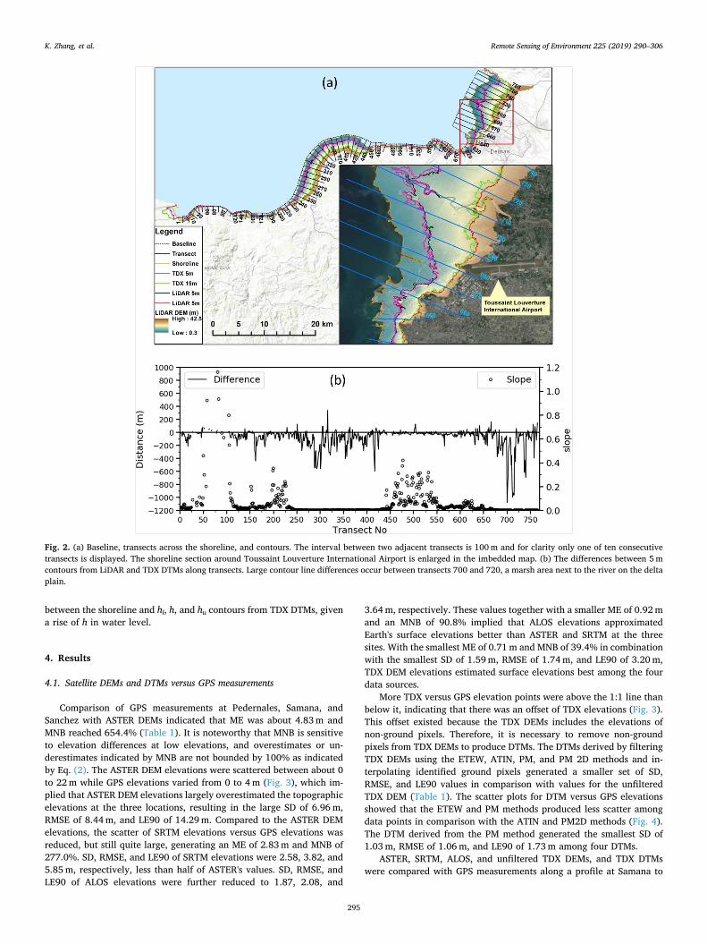
In estimating the uncertainty of the flood risk maps generated usingDTMs, it is important to quantify the horizontal position error of con-tour lines caused by vertical elevation uncertainty. The horizontal er-rors from TDX DTMs were examined by comparing the TDX and LiDARcontour lines in the same area, following a procedure used to mapshoreline and beach volume change (Leatherman and Clow, 1983;Robertson et al., 2018; Zhang and Robertson, 2001). First, an offshorebaseline that was approximately parallel to the contour lines was cre-ated in ArcGIS. Second, transects perpendicular to the baseline at agiven interval (e.g., 100m) were generated. Third, the distances be-tween the contour lines and the baseline along transects were calcu-lated to derive the differences between TDX and LiDAR contour lines(Fig. 2a).

The derivation of contour line position errors by comparing TDXand LiDAR contours only works for areas where both data sets exist.This method cannot be applied in areas where LiDAR data are notavailable. An alternative is to apply the elevation error derived by acomparison between TDX and LiDAR DTMs in overlapping coastal areasto the remaining coastal areas in Hispaniola, under the assumption thatthe elevation error of the remaining area is the same as the error in theoverlapping area. Given a TDX contour (yc), the systematic offset (m),the random error (σ) of the differences between TDX (yi) and LiDARDTM (xi) elevations, and the vertical error (δ) of LiDAR measurements,the lower (hl) and upper (hu) boundaries of the true contour (hc) areestimated by:

h y m c ch y m c c

l c

u c

= += + + + (10)

where parameters σ and δ are independent, c is a constant (e.g., 2 or 3),and σ can be estimated by SD, RMSE, NAMD, or LE90. A quality checkfor LiDAR data in the study area is not available. Since the RMSE errorof an airborne LiDAR survey is usually lower than 0.15m (Shan andToth, 2008), δ was set to be 0.15m in this study. The flood zone andassociated zones of uncertainty were estimated by the inundated areas

K. Zhang, et al. Remote Sensing of Environment 225 (2019) 290–306

294

between the shoreline and hl, h, and hu contours from TDX DTMs, givena rise of h in water level.

4. Results

4.1. Satellite DEMs and DTMs versus GPS measurements

Comparison of GPS measurements at Pedernales, Samana, andSanchez with ASTER DEMs indicated that ME was about 4.83m andMNB reached 654.4% (Table 1). It is noteworthy that MNB is sensitiveto elevation differences at low elevations, and overestimates or un-derestimates indicated by MNB are not bounded by 100% as indicatedby Eq. (2). The ASTER DEM elevations were scattered between about 0to 22m while GPS elevations varied from 0 to 4m (Fig. 3), which im-plied that ASTER DEM elevations largely overestimated the topographicelevations at the three locations, resulting in the large SD of 6.96m,RMSE of 8.44m, and LE90 of 14.29m. Compared to the ASTER DEMelevations, the scatter of SRTM elevations versus GPS elevations wasreduced, but still quite large, generating an ME of 2.83m and MNB of277.0%. SD, RMSE, and LE90 of SRTM elevations were 2.58, 3.82, and5.85m, respectively, less than half of ASTER's values. SD, RMSE, andLE90 of ALOS elevations were further reduced to 1.87, 2.08, and

3.64m, respectively. These values together with a smaller ME of 0.92mand an MNB of 90.8% implied that ALOS elevations approximatedEarth's surface elevations better than ASTER and SRTM at the threesites. With the smallest ME of 0.71m and MNB of 39.4% in combinationwith the smallest SD of 1.59m, RMSE of 1.74m, and LE90 of 3.20m,TDX DEM elevations estimated surface elevations best among the fourdata sources.

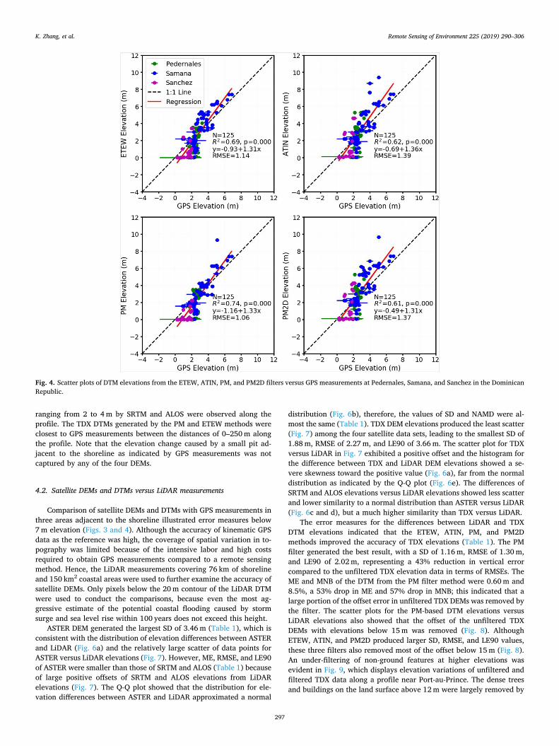
More TDX versus GPS elevation points were above the 1:1 line thanbelow it, indicating that there was an offset of TDX elevations (Fig. 3).This offset existed because the TDX DEMs includes the elevations ofnon-ground pixels. Therefore, it is necessary to remove non-groundpixels from TDX DEMs to produce DTMs. The DTMs derived by filteringTDX DEMs using the ETEW, ATIN, PM, and PM 2D methods and in-terpolating identified ground pixels generated a smaller set of SD,RMSE, and LE90 values in comparison with values for the unfilteredTDX DEM (Table 1). The scatter plots for DTM versus GPS elevationsshowed that the ETEW and PM methods produced less scatter amongdata points in comparison with the ATIN and PM2D methods (Fig. 4).The DTM derived from the PM method generated the smallest SD of1.03m, RMSE of 1.06m, and LE90 of 1.73m among four DTMs.

ASTER, SRTM, ALOS, and unfiltered TDX DEMs, and TDX DTMswere compared with GPS measurements along a profile at Samana to

Fig. 2. (a) Baseline, transects across the shoreline, and contours. The interval between two adjacent transects is 100m and for clarity only one of ten consecutivetransects is displayed. The shoreline section around Toussaint Louverture International Airport is enlarged in the imbedded map. (b) The differences between 5mcontours from LiDAR and TDX DTMs along transects. Large contour line differences occur between transects 700 and 720, a marsh area next to the river on the deltaplain.

K. Zhang, et al. Remote Sensing of Environment 225 (2019) 290–306

295

illustrate the spatial variation in the differences between satellite andGPS based elevations (Fig. 5). Between the distances of 0–250m fromshore to inland along the profile, ASTER elevations were much higherthan GPS elevations and the lowest ASTER elevation at 145m along theprofile differed by about 4m from the GPS elevations. Hence, the

application of filter methods to ASTER DEMs would not improve theestimates much because of large errors in DEM elevations and coarsehorizontal and vertical resolutions. SRTM and ALOS DEM elevationsalong the profile were closer to GPS elevations, outperforming ASTERDEMs. However, over- or underestimates of topographic elevations

Table 1Error measures. The representative row in the table is explained as follows. The row of “ASTER:GPS” shows the error measures of the differences between ASTERelevations and mean GPS elevations within ASTER grid cells. The row of “ETEW:GPS” shows the error measures of the differences between the elevations of theETEW filtered TDX DEM and mean GPS elevations within TDX grid cells. The row of “ASTER:LiDAR” shows the error measures of the differences between the ASTERand LiDAR elevations. The row of “ETEW:LiDAR” shows the error measures of the differences between the filtered TDX DEM and LiDAR DTM elevations. The row of“PM:LiDAR 3m” shows the error measures of the differences between 3m contours from the PM filtered TDX DEM and LiDAR DTM.

Comparison Number of samples ME (m) MD (m) MNB (%) SD (m) RMSE (m) NMAD (m) LE90 (m) R2

ASTER:GPS 95 4.83 3.01 654.4 6.96 8.44 8.33 14.29 0.31SRTM:GPS 95 2.83 3.00 277.0 2.58 3.82 2.29 5.85 0.00ALOS:GPS 95 0.92 0.20 90.8 1.87 2.08 1.63 3.64 0.10TDX:GPS 125 0.71 0.23 39.4 1.59 1.74 0.99 3.20 0.32ETEW:GPS 125 −0.09 −0.16 −11.3 1.14 1.14 1.21 1.81 0.69ATIN:GPS 125 0.28 0.08 4.1 1.37 1.39 1.19 2.15 0.62PM:GPS 125 −0.27 −0.22 −20.2 1.03 1.06 1.06 1.73 0.74PM2D:GPS 125 0.33 0.10 7.2 1.33 1.37 1.17 2.24 0.61ASTER:LiDAR 165,624 2.45 2.41 94.5 3.46 4.24 3.42 6.70 0.66SRTM:LiDAR 165,624 4.18 3.95 89.6 2.38 4.81 2.09 7.16 0.87ALOS:LiDAR 165,624 4.46 4.17 97.5 2.06 4.91 1.52 6.82 0.90TDX:LiDAR 1,022,699 1.27 0.69 20.0 1.88 2.27 1.12 3.66 0.92ETEW:LiDAR 1,022,699 0.76 0.57 12.5 1.47 1.66 0.96 2.51 0.94ATIN:LiDAR 1,022,699 0.80 0.59 12.8 1.32 1.55 0.94 2.29 0.95PM:LiDAR 1,022,699 0.60 0.40 8.5 1.16 1.30 0.81 2.02 0.96PM2D:LiDAR 1,022,699 0.88 0.63 14.3 1.33 1.60 1.03 2.57 0.95PM:LiDAR 3m 694 −49.2 −20.9 −5.8 104.4 115.3 52.9 172.9 0.99PM:LiDAR 5m 709 −75.0 −28.4 −6.5 144.5 162.7 48.7 211.1 0.99PM:LiDAR 10m 720 −59.9 −26.0 −3.3 123.0 136.7 51.4 202.9 1.00PM:LiDAR 15m 711 −66.4 −29.8 −1.7 115.5 133.2 56.9 232.8 1.00

Fig. 3. Scatter plots of ASTER, SRTM, ALOS, and TDXDEM elevations versus GPS measurements atPedernales, Samana, and Sanchez in the DominicanRepublic. The value of GPS elevation and horizontalbar of a data point represents the mean and standarddeviation of the GPS elevations within a DEM gridcell. Note that the ranges of ALOS and TDX DEMelevations are reduced by half of the ranges of ASTERand SRTM elevations to show elevation scatterednessbetter.

K. Zhang, et al. Remote Sensing of Environment 225 (2019) 290–306

296

ranging from 2 to 4m by SRTM and ALOS were observed along theprofile. The TDX DTMs generated by the PM and ETEW methods wereclosest to GPS measurements between the distances of 0–250m alongthe profile. Note that the elevation change caused by a small pit ad-jacent to the shoreline as indicated by GPS measurements was notcaptured by any of the four DEMs.

4.2. Satellite DEMs and DTMs versus LiDAR measurements

Comparison of satellite DEMs and DTMs with GPS measurements inthree areas adjacent to the shoreline illustrated error measures below7m elevation (Figs. 3 and 4). Although the accuracy of kinematic GPSdata as the reference was high, the coverage of spatial variation in to-pography was limited because of the intensive labor and high costsrequired to obtain GPS measurements compared to a remote sensingmethod. Hence, the LiDAR measurements covering 76 km of shorelineand 150 km2 coastal areas were used to further examine the accuracy ofsatellite DEMs. Only pixels below the 20m contour of the LiDAR DTMwere used to conduct the comparisons, because even the most ag-gressive estimate of the potential coastal flooding caused by stormsurge and sea level rise within 100 years does not exceed this height.

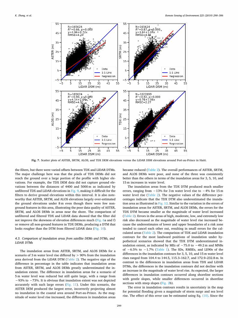
ASTER DEM generated the largest SD of 3.46m (Table 1), which isconsistent with the distribution of elevation differences between ASTERand LiDAR (Fig. 6a) and the relatively large scatter of data points forASTER versus LiDAR elevations (Fig. 7). However, ME, RMSE, and LE90of ASTER were smaller than those of SRTM and ALOS (Table 1) becauseof large positive offsets of SRTM and ALOS elevations from LiDARelevations (Fig. 7). The Q-Q plot showed that the distribution for ele-vation differences between ASTER and LiDAR approximated a normal

distribution (Fig. 6b), therefore, the values of SD and NAMD were al-most the same (Table 1). TDX DEM elevations produced the least scatter(Fig. 7) among the four satellite data sets, leading to the smallest SD of1.88m, RMSE of 2.27m, and LE90 of 3.66m. The scatter plot for TDXversus LiDAR in Fig. 7 exhibited a positive offset and the histogram forthe difference between TDX and LiDAR DEM elevations showed a se-vere skewness toward the positive value (Fig. 6a), far from the normaldistribution as indicated by the Q-Q plot (Fig. 6e). The differences ofSRTM and ALOS elevations versus LiDAR elevations showed less scatterand lower similarity to a normal distribution than ASTER versus LiDAR(Fig. 6c and d), but a much higher similarity than TDX versus LiDAR.

The error measures for the differences between LiDAR and TDXDTM elevations indicated that the ETEW, ATIN, PM, and PM2Dmethods improved the accuracy of TDX elevations (Table 1). The PMfilter generated the best result, with a SD of 1.16m, RMSE of 1.30m,and LE90 of 2.02m, representing a 43% reduction in vertical errorcompared to the unfiltered TDX elevation data in terms of RMSEs. TheME and MNB of the DTM from the PM filter method were 0.60m and8.5%, a 53% drop in ME and 57% drop in MNB; this indicated that alarge portion of the offset error in unfiltered TDX DEMs was removed bythe filter. The scatter plots for the PM-based DTM elevations versusLiDAR elevations also showed that the offset of the unfiltered TDXDEMs with elevations below 15m was removed (Fig. 8). AlthoughETEW, ATIN, and PM2D produced larger SD, RMSE, and LE90 values,these three filters also removed most of the offset below 15m (Fig. 8).An under-filtering of non-ground features at higher elevations wasevident in Fig. 9, which displays elevation variations of unfiltered andfiltered TDX data along a profile near Port-au-Prince. The dense treesand buildings on the land surface above 12m were largely removed by

Fig. 4. Scatter plots of DTM elevations from the ETEW, ATIN, PM, and PM2D filters versus GPS measurements at Pedernales, Samana, and Sanchez in the DominicanRepublic.

K. Zhang, et al. Remote Sensing of Environment 225 (2019) 290–306

297

Fig. 5. The aerial photograph, GPS points, grid cells of the SRTM DEM (upper panel), and the elevation profile across the GPS measurements (lower panel) at Samanain the Dominican Republic. The GPS measurements along the profile was generated by projecting the points within a 100m buffer zone to the profile line. The xcoordinate of the profile starts from shore (zero) and extends inland (left side of the aerial photograph).

Fig. 6. (a) The distribution of the elevation differences between the ASTER DEM, SRTM DEM, ALOS DEM, TDX DEMs, PM based DTM, and LiDAR DTM. Q-Q plots forthe differences between (b) ASTER and LiDAR, (c) SRTM and LiDAR, (d) ALOS and LiDAR, (e) TDX and LiDAR, and (f) PM based TDX and LiDAR elevations.

K. Zhang, et al. Remote Sensing of Environment 225 (2019) 290–306

298

the filters, but there were varied offsets between TDX and LIDAR DTMs.The major challenge here was that the pixels of TDX DEMs did notreach the ground over a large portion of the profile with higher ele-vations. For example, the TDX DEM data did not capture ground ele-vations between the distances of 4400 and 5000m as indicated byunfiltered TDX and LiDAR elevations in Fig. 9, making it difficult for thefilters to derive ground elevations within this interval. It is also note-worthy that ASTER, SRTM, and ALOS elevations largely over-estimatedthe ground elevations under 8m even though there were few non-ground features in this area, illustrating the poor data quality of ASTER,SRTM, and ALOS DEMs in areas near the shore. The comparison ofunfiltered and filtered TDX and LiDAR data showed that the filter didnot improve the skewness of elevation differences much (Fig. 6a and f)or remove all non-ground features in TDX DEMs, producing a DTM thatlooks rougher than the DTM from filtered LiDAR data (Fig. 10).

4.3. Comparison of inundation areas from satellite DEMs and DTMs, andLiDAR DTMs

The inundation areas from ASTER, SRTM, and ALOS DEMs for ascenario of 3m water level rise differed by>90% from the inundationarea derived from the LiDAR DTM (Table 2). The negative sign of thedifference in percentage in the table indicates that inundation areasfrom ASTER, SRTM, and ALOS DEMs greatly underestimated the in-undation extent. The difference in inundation areas for a scenario of5m water level was reduced but still quite large, with a range from−93% to −73%. It is obvious that inundation extent was not depictedaccurately with such large errors (Fig. 11). Under this scenario, theASTER DEM produced the largest error, incorrectly projecting almostno inundation in the coastal area around Port-au-Prince. As the mag-nitude of water level rise increased, the differences in inundation areas

became reduced (Table 2). The overall performances of ASTER, SRTM,and ALOS DEMs were poor, and none of the three was consistentlybetter than the others in terms of the inundation areas for 3, 5, 10, and15m increases in water level.

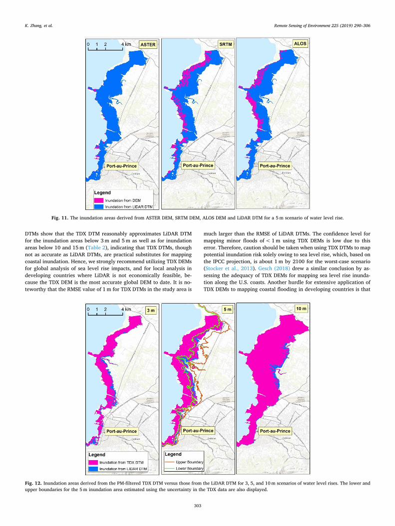
The inundation areas from the TDX DTM produced much smallererrors, ranging from −13% for 3m water level rise to −4% for 15mwater level rise (Table 2). The negative values of the difference per-centages indicate that the TDX DTM also underestimated the inunda-tion area as illustrated in Fig. 12. Similar to the variation in the errors ofinundation areas for ASTER, SRTM, and ALOS DEMs, the errors for theTDX DTM became smaller as the magnitude of water level increased(Table 2). Errors in the areas of high, moderate, low, and extremely lowrisk also decreased as the magnitude of water level rise increased be-cause the underestimates of lower and upper boundaries of a risk zonetended to cancel each other out, resulting in small errors for the cal-culated areas (Table 2). The comparison of TDX and LiDAR inundationcontours for the most landward positions of inundation under hy-pothetical scenarios showed that the TDX DTM underestimated in-undation extent, as indicated by MEs of −75.0 to −49.2m and MNBsof −6.5% to −1.7% (Table 1). The SDs, RMSEs, and LE90s of thedifferences in the inundation contours for 3, 5, 10, and 15m water levelrises ranged from 104.4 to 144.5, 115.3–162.7, and 172.9–232.8m. Incontrast to the differences in inundation areas from TDX and LiDARDTMs, the differences in the inundation contours did not decline withan increase in the magnitude of water level rise. As expected, the largerdifferences in inundation contours occurred along shoreline sectionswith gentle slopes, while smaller differences occurred in shorelinesections with steep slopes (Fig. 2b).

The error in inundation contours results in uncertainty in the mapfor potential flooding given a magnitude of storm surge and sea levelrise. The effect of this error can be estimated using Eq. (10). Since the

Fig. 7. Scatter plots of ASTER, SRTM, ALOS, and TDX DEM elevations versus the LiDAR DSM elevations around Port-au-Prince in Haiti.

K. Zhang, et al. Remote Sensing of Environment 225 (2019) 290–306

299

differences between TDX and LiDAR DTMs did not follow a normaldistribution (Fig. 6), the systematic offset (m) was estimated using theMD value, the random error (σ) was estimated using NAMD, δ was setto be 0.15m, and c was set to be 2. One example of the seaward andlandward extent attributable to errors between TDX and LiDAR DTMsfor the 5m inundation contour is illustrated in Fig. 12, where the dif-ference zone between TDX and LiDAR inundation contours wasbracketed by the boundaries of uncertainty.

5. Discussion

5.1. Accuracy analysis

The high accuracy of TDX DEM elevations versus GPS measure-ments that we observed (RMSE, 1.74m; LE90, 3.20m: Table 1) matcheswell with the accuracy assessment of TDX DEM with GPS data at aglobal scale (Wessel et al., 2018), who found RMSE of 1.71m and LE90of 2.59m when TDX DEMs were compared with benchmark GPSmeasurements in areas of medium development (Table 4 in Wessel et al.(2018)). Based on aerial photographs (Fig. 1), the land cover at Ped-ernales, Samana, and Sanchez GPS sites assessed in our study can becategorized as areas of medium development. By removing non-groundfeatures, TDX DTM derived by the PM filter resulted in 39% and 46%improvements in RMSE and LE90, respectively, indicating that similarfiltering of TDX DEMs should be conducted whenever possible.

The RMSE and LE90 from the comparison of TDX DEM elevationswith LiDAR measurements are 2.27 and 3.66m, respectively, higherthan the RMSE and LE90 from GPS measurements (Table 1). This is tobe expected because the LiDAR measurements cover extensive, 150 km2

areas that are occupied by many types of land cover, including marsh,forest, crop land, and low to high development. The LE90 value also

agrees with an overall LE90 of 3.49m derived by comparing TDX DEMswith> 144 million ICESat measurements (Rizzoli et al., 2017). Similarto the GPS surveyed areas, the TDX DTM from the PM filter improvedthe elevation accuracy by 43% and 45% in terms of RMSE and LE90,respectively.

The inundation polygons depicted by TDX and LiDAR DTMs mat-ched well spatially (Fig. 12) and the TDX and LiDAR inundation con-tours for these scenarios differed by distances that averaged< 75m.Error measures estimated from the coastal area around Port-au-Prince,Haiti can be used to quantify the flood mapping error using TDX DTMsfor the remaining areas of Hispaniola, under the assumption that theerrors are likely to be similar. This is a reasonable assumption becausethe LiDAR surveyed area includes most coastal land cover types inHispaniola. Transects of 1700m length along a profile near Port-au-Prince (Fig. 9) indicated no systematic offset between elevations fromTDX DEM and LiDAR DSM in open coastal areas. Several methods tomap the uncertainty for coastal inundation have been proposed (Gesch,2009; West et al., 2018). The method used in this study (i.e, Eq. (10))resembles the method developed by Gesch (2013), except that it alsoconsiders the systematic elevation offset in the filtered TDX DEM.

It is important to conduct error analysis by comparing TDX DEMelevations with GPS and LiDAR measurements with higher accuracy.The error measures allowed us to examine whether there was an offsetin TDX DEMs, and to produce lower and upper boundaries for the floodmaps due to elevation uncertainty. Kinematic GPS surveying is a con-venient way to collect accurate elevation data to verify TDX DEMs. Thesurvey in this study sampled about 20 elevation points within a30m×30m square. This method captured the spatial variation inelevations within a DEM grid cell, but reduced the survey efficiency. Itis probably better to survey the elevations along profiles perpendicularto contour lines, because sampling points will cover a large range of

Fig. 8. Scatter plots of DTM elevations produced with ETEW, ATIN, PM, and PM2D filters versus the LiDAR DTM elevations around Port-au-Prince in Haiti.

K. Zhang, et al. Remote Sensing of Environment 225 (2019) 290–306

300

elevations. The airborne LiDAR technology is more effective due to thelarge tracts of data collected, which include areas inaccessible toground surveyors. However, the cost and time of LiDAR survey and dataprocessing often prevent the application of LiDAR in developingcountries.

In contrast to TDX DEM, ASTER, SRTM, and ALOS DEMs producedlarger RMSE and LE90 errors and the performances of these three DEMswere not consistent. ALOS DEMs achieved a better accuracy than SRTMand ASTER DEMs in comparison with GPS measurements with eleva-tions below 7m, while at LiDAR elevations below 20m, ASTER had abetter accuracy due to a smaller offset than SRTM and ALOS DEMs.ASTER, SRTM, and ALOS DEMs generated larger discrepancies thanTDX DTMs in delineation of inundation areas (Table 2) and contours(Fig. 11) for 3, 5, 10, and 15m. Similar to elevation accuracy, none ofthe three was consistently better than the others in the calculation ofinundation areas.

When ASTER and ALOS DEMs from the analysis of stereoscopicoptical images as well as SRTM and TDX DEMs from radar were com-pared in pairs, both the ALOS sensor, which generated higher resolution(2.5 m) images than 15m resolution imagery from ASTER (Abramset al., 2010; Tadono et al., 2014), and the TDX sensors, with a longerradar baseline from two tandem satellites than the baseline from asingle antenna in the space shuttle (Farr et al., 2007; Gruber et al.,2012), improve the elevation accuracy of the data. When compared onthe basis of GPS measurements, both ALOS versus ASTER DEMs andTDX versus SRTM DEMs showed a better response to GPS elevationchanges (Fig. 3). The comparison of DEMs with LiDAR measurementsshowed a similar pattern (Fig. 7), although ALOS DEM generated a

larger RMSE value than ASTER DEM due to an offset. This offset can beremoved if sufficient elevation measurements (e.g. from GPS) withhigher accuracy at sample sites are available.

Numerous studies in developing countries have employed opensource ASTER and SRTM DEMs to map the potential flooding that willresult from storm surges and sea level rise on a local scale (Aleem andAina, 2014; Demirkesen et al., 2007; Ho et al., 2010; Kuleli, 2010;Pramanik et al., 2015; Refaat and Eldeberky, 2016). On a global scale,most studies that document potential flood risk in coastal cities or zoneshave used SRTM DEMs as well (Hallegatte et al., 2013; Hinkel et al.,2014; McGranahan et al., 2007). Such studies suffer the followingcommon problems: (1) most of them did not conduct accuracy analyses,and (2) SRTM and ASTER data grossly underestimated inundationareas, especially for coastal lands below 5m elevation. As a result, theimpacted population, property, and facilities in flood-vulnerable areaswere also underestimated. In the coastal area around Port-au-Prince,this underestimate was remarkable (Table 2 and Fig. 11), as the in-undation areas below 5m from SRTM and ASTER DEMs were 5 and 15times smaller, respectively, in comparison with the LiDAR-based in-undation area. Similar underestimates of inundation areas by SRTM andASTER DEMs were also found on the local scale in Nigeria (van deSande et al., 2012), Indonesia (Griffin et al., 2015), Poland (Walczaket al., 2016), and England (Yunus et al., 2016), and on the national levelin the U.S. (Kulp and Strauss, 2016). One could argue that the RMSE inASTER and SRTM DEMs can be improved by removing offsets throughcomparison of DEMs with reference data of higher accuracy. Un-fortunately, the offsets may not be systematic as indicated by the scatterplot between ASTER and LiDAR DEMs in Fig. 7. Even if the offsets seem

Fig. 9. Aerial photograph (upper panel) and the elevation profile (lower panel) near Port-au-Prince in Haiti. The profile starts from a location close to shore with an xcoordinate of zero and extends inland.

K. Zhang, et al. Remote Sensing of Environment 225 (2019) 290–306

301

systematic, as indicated by scatter plots for SRTM and ALOS versusLiDAR, there is no guarantee that the offsets estimated at Port-au-Princecould be applied to places other than the study area.

In addition, inconsistent performances by ASTER, SRTM, and ALOS

DEMs in depicting inundation areas for low and high water level risescenarios makes it difficult to select which of the three is more suitablefor mapping potential coastal inundation. By contrast, the differences inestimated inundation areas around Port-au-Prince from TDX and LiDAR

Fig. 10. TDX DEM, LiDAR DSM, TDX DTM, and LiDAR DTM for the area near Port-au-Prince in Haiti.

Table 2Inundation areas generated from ASTER, SRTM, and ALOS DEMs, and TDX and LiDAR DTMs for hypothetical water level rise (WLR) scenarios of 3, 5, 10, and 15m.The TDX DTM was generated by the PM filter. The differences in percentage between the areas from ASTER, SRTM, ALOS, and TDX, and the area from LiDAR werelisted in parentheses.

WLR Scenarios (m) ASTER in km2(%) SRTM in km2(%) ALOS in km2(%) TDX in km2(%) LiDAR (km2) Risk class Risk area (TDX/LiDAR, km2/km2/(%))

3 0.7 (−98) 2.1 (−93) 1.6 (−95) 26.0 (−13) 30.0 High 26.0/30.0 (−13)5 3.3 (−93) 11.0 (−73) 9.0 (−82) 44.7 (−11) 50.0 Moderate 18.7/20.0 (−7)10 68.7 (−22) 56.9 (−35) 55.1 (−38) 83.5 (−5) 88.2 Low 38.8/38.2 (2)15 111.3 (−7) 91.2 (−24) 90.9 (−24) 114.9 (−4) 119.8 Extremely low 31.4/31.6 (−1)

K. Zhang, et al. Remote Sensing of Environment 225 (2019) 290–306

302

DTMs show that the TDX DTM reasonably approximates LiDAR DTMfor the inundation areas below 3m and 5m as well as for inundationareas below 10 and 15m (Table 2), indicating that TDX DTMs, thoughnot as accurate as LiDAR DTMs, are practical substitutes for mappingcoastal inundation. Hence, we strongly recommend utilizing TDX DEMsfor global analysis of sea level rise impacts, and for local analysis indeveloping countries where LiDAR is not economically feasible, be-cause the TDX DEM is the most accurate global DEM to date. It is no-teworthy that the RMSE value of 1m for TDX DTMs in the study area is

much larger than the RMSE of LiDAR DTMs. The confidence level formapping minor floods of< 1m using TDX DEMs is low due to thiserror. Therefore, caution should be taken when using TDX DTMs to mappotential inundation risk solely owing to sea level rise, which, based onthe IPCC projection, is about 1m by 2100 for the worst-case scenario(Stocker et al., 2013). Gesch (2018) drew a similar conclusion by as-sessing the adequacy of TDX DEMs for mapping sea level rise inunda-tion along the U.S. coasts. Another hurdle for extensive application ofTDX DEMs to mapping coastal flooding in developing countries is that

Fig. 11. The inundation areas derived from ASTER DEM, SRTM DEM, ALOS DEM and LiDAR DTM for a 5m scenario of water level rise.

Fig. 12. Inundation areas derived from the PM-filtered TDX DTM versus those from the LiDAR DTM for 3, 5, and 10m scenarios of water level rises. The lower andupper boundaries for the 5m inundation area estimated using the uncertainty in the TDX data are also displayed.

K. Zhang, et al. Remote Sensing of Environment 225 (2019) 290–306

303

TDX 12m DEMs are not freely available, although DLR released TDX90m DEMs to the public in October 2018. Comparison of TDX 12m and90m DEMs at Port-au-Prince, Haiti showed that 90m DEMs capturedmajor elevation change patterns, but smoothed out many local eleva-tion variations because of resolution reduction. Due to this smoothingeffect, the filtering of 90m DEMs probably provides little improvementof DTM accuracy, thereby greatly increasing uncertainty in depictinginundation zones.

5.2. Filtering of TDX DEMs

It has been demonstrated that the DTMs generated by filtering andinterpolating TDX DEMs resulted in approximately 40% improvementin estimates of ground elevation. Therefore, filtering methods areneeded if TDX DEMs are to be used to map coastal flood hazards ac-curately. Among the four tested filtering methods, the PM filter using aone-dimensional structure element generated the best results becausethis filter effectively preserved river banks, low coastal cliffs, and gentlysloping terrain features such as floodplains within the study area(Zhang et al., 2003; Zhang and Whitman, 2005). By contrast, the ETEWand ATIN methods incorrectly removed ground pixels bordering riverbanks, as well as low coastal cliffs where sharp elevation changes oc-curred. Likewise, the PM2D filter is less effective in retaining geo-morphic features compared to the PM filter, due to its use of a two-dimensional square or circular structure element.

The filtering methods for LiDAR measurements can either be di-rectly applied to the TDX DEMs (this study) or modified to fit TDXDEMs (Geiß et al., 2015; Schreyer et al., 2016) because these filters arebased on a similar assumption for separation of ground and non-groundpixels. The assumption is that changes in the elevations of ground pixelsare gradual and spatially correlated within a local window, whilechanges in elevations between ground and non-ground features areabrupt and poorly correlated. However, due to footprint sizes and datapoint density, TDX and LiDAR data differ remarkably in terms of theirlikelihood of penetrating through vegetation. LiDAR can reach theground even in dense coastal forests such as mangroves and tropicalhardwoods because of its small footprint size and high spatial mea-surement density (Zhang et al., 2008). By contrast, TDX measurementsfrom the X-band radar wave cannot penetrate through dense coastalforests to reach the ground, making it impractical to separate groundelevations from non-ground elevations in these types of land cover. Inheavily-built metropolitan areas, where streets are not much wider thanthe 12m spatial resolution of TDX DEMs, shadow effects and the mixingof different objects in a TDX DEM pixel also prevent consistent groundmeasurements. In medium-developed and sparse or patchily vegetatedareas, ground and non-ground features are generally separable in TDXDEMs (Rossi and Gernhardt, 2013; Schreyer and Lakes, 2016), and it isin such landscapes that TDX DEMs can provide reliable DTMs formapping flood impacts.

Even in medium-developed or patchily vegetated areas, the im-provement in identification of ground pixels by modifying the existingfiltering method to fit the characteristics of TDX DEMs deserves furtherstudy. For example, the TDX sensor did not capture the ground mea-surements between the distances 4400 and 5000m along a profile nearPort-au-Prince (Fig. 9), resulting in an overestimate of ground eleva-tions in the filtered data. This overestimate caused corresponding un-derestimates of the potential flood areas shown in Fig. 12. A possiblestrategy to handle this large spatial gap in ground measurements is toselect high quality, well separated ground pixels from the TDX DEMs asseed points in the first step of forming the initial ground pixel set andgenerating an initial ground surface by interpolating ground pixels. Thenext step would be to iteratively search the candidate pixels and addcandidates to the ground set by comparing the distances from candidatepixels to ground surface. Manual editing of automatically selected seedpixels may be needed to ensure that the seeds are reliable because theeffect of the seed pixels is magnified in adding more ground pixels

through an iterative process (Zhao et al., 2016). The land cover data,especially from satellite platforms such as Sentinel that collect imageswith a spatial resolution similar to TDX DEMs, should be incorporatedinto the filtering process for selecting seed ground pixels and de-termining filtering parameters.

6. Conclusions

The elevation accuracy of ASTER, SRTM, ALOS, and TDX DEMs forHispaniola were examined against> 2000 RTK GPS measurements inthe Dominican Republic and 150 km2 LiDAR data in Haiti to determineif these DEMs are appropriate for mapping coastal flood risk. Thecomparison between DEM elevations and GPS measurements below 7melevations showed that the TDX DEMs achieved the best accuracy,generating the smallest SD of 1.59m, RMSE of 1.74m, and LE90 of3.20m. ASTER DEMs had the lowest accuracy, generating the largestSD of 6.96m, RMSE of 8.44m, and LE90 of 14.29m, while SRTM andALOS DEMs were intermediate in accuracy with 2.58 and 1.87m SDs,3.82 and 2.08m RMSEs, and 5.58 and 3.64m LE90s, respectively. Theoffsets generated by non-ground features in TDX DEMs were largelyremoved by the ETEW, ATIN, PM, and PM2D filters. The PM filterproduced the best results, reducing SD to 1.03m, RMSE to 1.06m, andLE90 to 1.73m, making 39%–46% improvement over unfiltered data.

The comparison between DEM elevations and LiDAR measurementsbelow 20m indicated a similar pattern in accuracy from DEMs versusGPS measurements. TDX DEMs had the best accuracy, generating thesmallest SD of 1.88m, RMSE of 2.27m, and LE90 of 3.66m. However,SRTM DEMs produced the largest errors, with RMSE of 4.81m, andLE90 of 7.16m due to an offset in the data, while ASTER and ALOSDEMs generated slightly lower errors than SRTM DEMs. The errormeasures from DEM versus LiDAR elevations were larger than the errormeasures from DEM versus GPS elevations because LiDAR measure-ments covered a large area of 150 km2, where there were multiple typesof land cover including marsh, forest, crop land, and low to high de-velopment. It is better to estimate the statistical parameters for eleva-tion differences using MD and NMAD than using ME and SD because,except for ASTER, the differences between satellite-derived and LiDARelevations did not follow a normal distribution. The comparison ofDTMs from the ETEW, ATIN, PM, and PM2D filters showed that the PMfilter produced the best result, with a SD of 1.16m, RMSE of 1.30m,and LE90 of 2.02m, resulting in a 43% improvement in RMSE afterfiltering.

The inundation areas from the TDX DTM for scenarios of 3, 5, 10,and 15m water level rise produced errors between −13% and −4%compared to the inundation areas from LiDAR DTM. The error in esti-mates of inundated areas decreased as the magnitude of water level riseincreased, because the area of inundation increased as water level rose,but the error of the inundation edge did not decrease. The high, mod-erate, low, and extremely low risk zones derived from TDX and LiDARDTMs differed by −13%, −7%, 2%, and −1%, respectively, for a150 km2 area with elevations below 20m. The TDX DTM under-estimated the inundation extent as indicated by MEs of −75.0 to−49.2m and SDs, RSMEs, and LE90s of the differences in inundationextent for 3, 5, 10, and 15m water level rise ranged from 104.4 to144.5, 115.3–162.7, and 172.9–232.8m, respectively. Therefore, TDXDTMs provide an effective approximation of LiDAR DTMs for coastalflood mapping in the area where LiDAR data are not available. Bycontrast, the inundation areas from ASTER, SRTM, and ALOS DEMs for3 and 5m water level rise scenarios had −98% to −73% of differencescompared to the inundation areas from the LiDAR DTM. The inundationareas below 5m from SRTM and ASTER DEMs were 5 and 15 timessmaller than the inundated area based on LiDAR. Among ASTER, SRTM,and ALOS DEMs, no single data source consistently performed the bestin defining inundation areas for 3, 5, 10, and 15m scenarios of waterlevel rise. We strongly recommend that TDX DEMs be utilized to con-duct both global and local analysis of sea level and storm surge impacts

K. Zhang, et al. Remote Sensing of Environment 225 (2019) 290–306

304

in developing countries.The DTMs generated by filtering and interpolating TDX DEMs im-

proved the accuracy of ground elevations by about 40% along the coastnear Port-au-Prince, Haiti, thereby greatly reducing the uncertainty inmapping coastal inundation caused by sea level rise and storm surges.Therefore, filtering methods must be applied to TDX DEMs to deriveDTMs for accurately delineating coastal flood hazard zones. However,the effectiveness of filtering is limited by the spatial resolution of TDXDEMs for locations where dense vegetation and buildings prevent radarwaves from reaching the ground. Though filtering methods employed inthis study worked well for medium-developed or patchily vegetatedareas, the existing filters need to be improved, or a new filter that fitsthe characteristics of TDX DEMs needs to be developed to generatebetter DTMs in the future.

Acknowledgements

This work was supported by “Development of an Integrated CoastalInundation Forecast Demonstration System in the Caribbean Region –Pilot Project for the Dominican Republic and Haiti” sponsored by theUnited States Agency for International Development (USAID) andNational Oceanic and Atmospheric Administration. The GermanAerospace Center provided TanDEM-X DEM data for Hispaniolathrough the project “Developing Hurricane Storm Surge Planning andForecasting Capabilities for Haiti and the Dominican Republic UsingTanDEM-X DEMs” (Proposal ID: DEM_HYDR0550). We thank theUSAID's Office of U.S. Foreign Disaster Assistance (USAID/OFDA) fortheir support to conduct the RTK GPS survey in Hispaniola, through theFlorida International University's Disaster Risk Reduction Program. Weare also grateful to Dr. Dar Roberts, Associate Editor and three anon-ymous reviewers for providing valuable comments which have beenvery helpful in improving the manuscript.

References

Abrams, M., Bailey, B., Tsu, H., Hato, M., 2010. The aster global dem. Photogramm. Eng.Remote Sensing 76, 344–348.

Aleem, K.F., Aina, Y.A., 2014. Using SRTM and GDEM2 data for assessing vulnerability tocoastal flooding due to sea level rise in Lagos: a comparative study. FUTY J. Environ.8, 53–64.

Axelsson, P., 2000. DEM generation from laser scanner data using adaptive TIN models.Int. Arch. Photogramm. Remote Sens. 33, 110–117.

Bamber, J.L., Riva, R.E.M., Vermeersen, B.L.A., Lebrocq, A.M., 2009. Reassessment of thepotential of the West Antarctic ice sheet. Science 324, 901–904. https://doi.org/10.1126/science.1169335. (80-. ).

Boulton, S.J., Stokes, M., 2018. Which DEM is best for analyzing fluvial landscape de-velopment in mountainous terrains? Geomorphology 310, 168–187.

Cui, Z., Zhang, K., Zhang, C., Yan, J., Chen, S.C., 2013. A GUI based LIDAR data pro-cessing system for model generation and mapping. In: Proceedings of the 1st ACMSIGSPATIAL International Workshop on MapInteraction. ACM, Orlando, pp. 40–43.

Davis, J., 2002. Statistics and Data Analysis in Geology, 3rd ed. John Willey & Sons, Inc,New York.

Demirkesen, A.C., Evrendilek, F., Berberoglu, S., Kilic, S., 2007. Coastal flood risk analysisusing Landsat-7 ETM+ imagery and SRTM DEM: a case study of Izmir, Turkey.Environ. Monit. Assess. 131, 293–300.

Demirkesen, A.C., Evrendilek, F., Berberoglu, S., 2008. Quantifying coastal inundationvulnerability of Turkey to sea-level rise. Environ. Monit. Assess. 138, 101–106.

Farr, T.G., Rosen, P.A., Caro, E., Crippen, R., Duren, R., Hensley, S., Kobrick, M., Paller,M., Rodriguez, E., Roth, L., 2007. The shuttle radar topography mission. Rev.Geophys. 45. https://doi.org/10.1029/2005RG000183.

Franzen, D.W., Clay, D., Shanahan, J.F., 2011. Collecting and analyzing soil spatial in-formation using kriging and inverse distance. In: Clay, D.E., Shanahan, J.F. (Eds.),GIS Appl. Agric. Nutr. Manag. Energy Effic. Taylor Fr, New York, NY, USA, pp. 61–80.

Geiß, C., Wurm, M., Breunig, M., Felbier, A., Taubenböck, H., 2015. Normalization ofTanDEM-X DSM data in urban environments with morphological filters. IEEE Trans.Geosci. Remote Sens. 53, 4348–4362.

Gesch, D.B., 2009. Analysis of lidar elevation data for improved identification and deli-neation of lands vulnerable to sea-level rise. J. Coast. Res. 49–58.

Gesch, D.B., 2013. Consideration of vertical uncertainty in elevation-based sea-level riseassessments: Mobile Bay, Alabama case study. J. Coast. Res. 63, 197–210.

Gesch, D.B., 2018. Best practices for elevation-based assessments of sea-level rise andcoastal flooding exposure. Front. Earth Sci. 6, 230.

Griffin, J., Latief, H., Kongko, W., Harig, S., Horspool, N., Hanung, R., Rojali, A., Maher,N., Fuchs, A., Hossen, J., 2015. An evaluation of onshore digital elevation models formodeling tsunami inundation zones. Front. Earth Sci. 3, 32.

Gruber, A., Wessel, B., Huber, M., Roth, A., 2012. Operational TanDEM-X DEM calibra-tion and first validation results. ISPRS J. Photogramm. Remote Sens. 73, 924–2716.

Hallegatte, S., Green, C., Nicholls, R.J., Corfee-Morlot, J., 2013. Future flood losses inmajor coastal cities. Nat. Clim. Chang. 3, 802.

Hinkel, J., Lincke, D., Vafeidis, A.T., Perrette, M., Nicholls, R.J., Tol, R.S.J., Marzeion, B.,Fettweis, X., Ionescu, C., Levermann, A., 2014. Coastal flood damage and adaptationcosts under 21st century sea-level rise. Proc. Natl. Acad. Sci. 111, 3292–3297.

Ho, L.T.K., Umitsu, M., Yamaguchi, Y., 2010. Flood hazard mapping by satellite imagesand SRTM DEM in the Vu Gia–Thu Bon alluvial plain, Central Vietnam. Int. Arch.Photogramm. Remote. Sens. Spat. Inf. Sci. 38, 275–280.

Höhle, J., Höhle, M., 2009. Accuracy assessment of digital elevation models by means ofrobust statistical methods. ISPRS J. Photogramm. Remote Sens. 64, 398–406.

ITRF, 2013. ITRS and WGS84. ftp://itrf.ensg.ign.fr/pub/itrf/WGS84.TXT, Accessed date:3 November 2018.

Knutson, T.R., McBride, J.L., Chan, J., Emanuel, K., Holland, G., Landsea, C., Held, I.,Kossin, J.P., Srivastava, A.K., Sugi, M., 2010. Tropical cyclones and climate change.Nat. Geosci. 3, 157.

Komar, P.D., 1998. Beach Processes and Sedimentation. Prentice Hall, Upper SaddleRiver, New Jersey.

Krieger, G., Moreira, A., Fiedler, H., Hajnsek, I., Werner, M., Younis, M., Zink, M., 2007.TanDEM-X: a satellite formation for high-resolution SAR interferometry. IEEE Trans.Geosci. Remote Sens. 45, 3317–3341.

Krivoruchko, K., 2012. Empirical Bayesian Kriging. ArcUser Fall 2012. pp. 6–10.Kuleli, T., 2010. City-based risk assessment of sea level rise using topographic and census

data for the Turkish coastal zone. Estuar. Coasts 33, 640–651.Kulp, S., Strauss, B.H., 2016. Global DEM errors underpredict coastal vulnerability to sea

level rise and flooding. Front. Earth Sci. 4, 36.Leatherman, S.P., Clow, B., 1983. UMD shoreline mapping project. IEEE Geosci. Remote

Sens. Soc. Newsl. 22, 5–8.McGranahan, G., Balk, D., Anderson, B., 2007. The rising tide: assessing the risks of cli-

mate change and human settlements in low elevation coastal zones. Environ. Urban.19, 17–37.

Mirzaei, R., Sakizadeh, M., 2016. Comparison of interpolation methods for the estimationof groundwater contamination in Andimeshk-Shush Plain, Southwest of Iran.Environ. Sci. Pollut. Res. 23, 2758–2769.

Neumann, B., Vafeidis, A.T., Zimmermann, J., Nicholls, R.J., 2015. Future coastal po-pulation growth and exposure to sea-level rise and coastal flooding-a global assess-ment. PLoS One 10, e0118571. https://doi.org/10.1371/journal.pone.0118571.

Nicholls, R.J., Marinova, N., Lowe, J.A., Brown, S., Vellinga, P., De Gusmao, D., Hinkel,J., Tol, R.S.J., 2011. Sea-level rise and its possible impacts given a ‘beyond 4 C world’in the twenty-first century. Philos. Trans. R. Soc. London A Math. Phys. Eng. Sci. 369,161–181.

Pavlis, N.K., Holmes, S.A., Kenyon, S.C., Factor, J.K., 2012. The development and eva-luation of the earth gravitational model 2008 (EGM2008). J. Geophys. Res. SolidEarth 117. https://doi.org/10.1029/2011JB008916.

Pramanik, M.K., Biswas, S.S., Mukherjee, T., Roy, A.K., Pal, R., Mondal, B., 2015. Sealevel rise and coastal vulnerability along the eastern coast of India through geospatialtechnologies. J. Geophys. Remote Sens. 4, 145. https://doi.org/10.4172/2469-4134.1000145.

Refaat, M.M., Eldeberky, Y., 2016. Assessment of coastal inundation due to sea-level risealong the Mediterranean Coast of Egypt. Mar. Geod. 39, 290–304.

Rizzoli, P., Martone, M., Gonzalez, C., Wecklich, C., Tridon, D.B., Bräutigam, B.,Bachmann, M., Schulze, D., Fritz, T., Huber, M., 2017. Generation and performanceassessment of the global TanDEM-X digital elevation model. ISPRS J. Photogramm.Remote Sens. 132, 119–139.

Roberts, J.D., Voss, J.D., Knight, B., 2014. The association of ambient air pollution andphysical inactivity in the United States. PLoS One 9. https://doi.org/10.1371/journal.pone.0090143.

Robertson, Q., Dunkin, L., Dong, Z., Wozencraft, J., Zhang, K., 2018. Florida and US eastcoast beach change metrics derived from LiDAR data utilizing ArcGIS Python basedtools. In: Botero, C.M., Cervantes, O., Finkl, C.W. (Eds.), Beach Management Tools-Concepts, Methodologies and Case Studies. Springer International Publishing AG,Cham, pp. 239–258.

Rodriguez, M.O.C., Barba, D.C., 2009. The Hispaniola fluvial system and its morphos-tructural context. Phys. Geogr. 30, 453–478.

Rodriguez, E., Morris, C.S., Belz, J.E., 2006. A global assessment of the SRTM perfor-mance. Photogramm. Eng. Remote. Sens. 72, 249–260.

Rossi, C., Gernhardt, S., 2013. Urban DEM generation, analysis and enhancements usingTanDEM-X. ISPRS J. Photogramm. Remote Sens. 85, 120–131.

Schreyer, J., Lakes, T., 2016. Deriving and evaluating city-wide vegetation heights from aTanDEM-X DEM. Remote Sens. 8, 940.

Schreyer, J., Geiß, C., Lakes, T., 2016. TanDEM-X for large-area modeling of urban ve-getation height: evidence from Berlin, Germany. IEEE J. Sel. Top. Appl. Earth Obs.Remote Sens. 9, 1876–1887.

Shan, J., Toth, C.K., 2008. Topographic Laser Ranging and Scanning: Principles andProcessing. CRC Press, Boca Raton.

Stocker, T.F., Qin, D., Plattner, G.K., Tignor, M., Allen, S.K., Boschung, J., Nauels, A., Xia,Y., Bex, V., Midgley, P.M., 2013. Climate change 2013: the physical science basis:Working Group I contribution to the Fifth assessment report of the IntergovernmentalPanel on Climate Change. Cambridge University Press.

Sweet, W.V., Kopp, R.E., Weaver, C.P., Obeysekera, J., Horton, R.M., Thieler, E.R., Zervas,C., 2017. Global and Regional Sea Level Rise Scenarios for the United States. NationalOceanic and Atmospheric Administration, Silver Spring.

Tachikawa, T., Hato, M., Kaku, M., Iwasaki, A., 2011a. Characteristics of ASTER GDEMversion 2. In: Geoscience and Remote Sensing Symposium (IGARSS), 2011 IEEEInternational. IEEE, Vancouver, pp. 3657–3660.

K. Zhang, et al. Remote Sensing of Environment 225 (2019) 290–306

305

Tachikawa, T., Kaku, M., Iwasaki, A., Gesch, D., Oimoen, M., Zhang, Z., Danielson, J.,Krieger, T., Curtis, B., Haase, J., NASA, 2011b. ASTER Global Digital Elevation ModelVersion 2–Summary of Validation Results. https://ssl.jspacesystems.or.jp/ersdac/GDEM/ver2Validation/Summary_GDEM2_validation_report_final.pdf, Accessed date:3 November 2018.

Tadono, T., Ishida, H., Oda, F., Naito, S., Minakawa, K., Iwamoto, H., 2014. Precise globalDEM generation by ALOS PRISM. ISPRS Ann. Photogramm. Remote Sens. Spat. Inf.Sci. 2, 71.

Tadono, T., Nagai, H., Ishida, H., Oda, F., Naito, S., Minakawa, K., Iwamoto, H., 2016.Generation of the 30 m-mesh global digital surface model by ALOS PRISM. Int. Arch.Photogramm. Remote. Sens. Spat. Inf. Sci. 41.

Takaku, J., Tadono, T., 2009. PRISM on-orbit geometric calibration and DSM perfor-mance. IEEE Trans. Geosci. Remote Sens. 47, 4060–4073.

Takaku, J., Tadono, T., 2017. Quality updates of ‘AW3D’ global DSM generated fromALOS PRISM, in: Geoscience and remote sensing symposium (IGARSS). In: 2017 IEEEInternational. IEEE, Fort Worth, pp. 5666–5669.

Takaku, J., Tadono, T., Tsutsui, K., 2014. Generation of high resolution global DSM fromALOS PRISM. Int. Arch. Photogramm. Remote. Sens. Spat. Inf. Sci. 40, 243.

Takaku, J., Tadono, T., Tsutsui, K., Ichikawa, M., 2016. Validation of "AW3D" global DSMgenerated from Alos Prism. ISPRS Ann. Photogramm. Remote Sens. Spat. Inf. Sci.3, 25.

United Nations, 2017. World population prospects: 2017 revision, data booklet. ST/ESA/SER.A/401. https://population.un.org/wpp/Publications/, Accessed date: 3November 2018.

Van Aardt, J.A.N., McKeown, D., Faulring, J., Raqueño, N., Casterline, M., Renschler, C.,Eguchi, R., Messinger, D., Krzaczek, R., Cavillia, S., 2011. Geospatial disaster re-sponse during the Haiti earthquake: a case study spanning airborne deployment, datacollection, transfer, processing, and dissemination. Photogramm. Eng. RemoteSensing 77, 943–952.

van de Sande, B., Lansen, J., Hoyng, C., 2012. Sensitivity of coastal flood risk assessmentsto digital elevation models. Water 4, 568–579.

Walczak, Z., Sojka, M., Wróżyński, R., Laks, I., 2016. Estimation of polder retention ca-pacity based on ASTER, SRTM and LIDAR DEMs: the case of Majdany Polder (WestPoland). Water 8, 230.

Wessel, B., 2016. TanDEM-X Ground Segment–DEM Products Specification Document.German Space Center.

Wessel, B., Huber, M., Wohlfart, C., Marschalk, U., Kosmann, D., Roth, A., 2018. Accuracyassessment of the global TanDEM-X digital elevation model with GPS data. ISPRS J.

Photogramm. Remote Sens. 1–12.West, H., Horswell, M., Quinn, N., 2018. Exploring the sensitivity of coastal inundation

modelling to DEM vertical error. Int. J. Geogr. Inf. Sci. 32, 1172–1193.Wilson, J.S., Brothers, T.S., Marcano, E.J., 2001. Remote sensing of spatial and temporal

vegetation dynamics in Hispaniola: a comparison of Haiti and the DominicanRepublic. Geocarto Int 16, 7–18.

Wolf, P.R., Dewitt, B.A., Wilkinson, B.E., 2000. Elements of Photogrammetry: WithApplications in GIS. McGraw-Hill, New York.

Yunus, A.P., Avtar, R., Kraines, S., Yamamuro, M., Lindberg, F., Grimmond, C.S.B., 2016.Uncertainties in tidally adjusted estimates of sea level rise flooding (bathtub model)for the Greater London. Remote Sens. 8, 366.

Zhang, K., 2007. Airborne LiDAR data processing and analysis tools. In: AGU Fall MeetingAbstracts, . http://adsabs.harvard.edu/abs/2007AGUFM.H52E..01Z, Accessed date:8 November 2018.

Zhang, K., 2011. Analysis of non-linear inundation from sea-level rise using LIDAR data: acase study for South Florida. Clim. Chang. 106, 537–565.

Zhang, K., Robertson, W., 2001. Historical shoreline mapping and analysis with metricmapping. In: Coastal GeoTools'01. Proceedings of the 2nd Biennial Coastal GeoToolsConference, . http://coastalgeotools.org/wp-content/uploads/GeoTools2011_program.pdf, Accessed date: 8 November 2018.

Zhang, K., Whitman, D., 2005. Comparison of three algorithms for filtering airborne lidardata. Photogramm. Eng. Remote. Sens. 71, 313–324.

Zhang, K., Chen, S.-C., Whitman, D., Shyu, M.-L., Yan, J., Zhang, C., 2003. A progressivemorphological filter for removing nonground measurements from airborne LIDARdata. IEEE Trans. Geosci. Remote Sens. 41, 872–882.

Zhang, K., Simard, M., Ross, M., Rivera-Monroy, V.H., Houle, P., Ruiz, P., Twilley, R.R.,Whelan, K., 2008. Airborne laser scanning quantification of disturbances from hur-ricanes and lightning strikes to mangrove forests in Everglades National Park, USA.Sensors 8, 2262–2292.

Zhang, K., Dittmar, J., Ross, M., Bergh, C., 2011. Assessment of sea level rise impacts onhuman population and real property in the Florida Keys. Clim. Chang. 107, 129–146.

Zhao, X., Guo, Q., Su, Y., Xue, B., 2016. Improved progressive TIN densification filteringalgorithm for airborne LiDAR data in forested areas. ISPRS J. Photogramm. RemoteSens. 117, 79–91.

Zink, M., Bachmann, M., Brautigam, B., Fritz, T., Hajnsek, I., Moreira, A., Wessel, B.,Krieger, G., 2014. TanDEM-X: the new global DEM takes shape. IEEE Geosci. RemoteSens. Mag. 2, 8–23.

K. Zhang, et al. Remote Sensing of Environment 225 (2019) 290–306

306