dems of difference - enlighteneprints.gla.ac.uk/114527/1/williams 2012 dems of difference.pdf ·...

British Society for Geomorphology Geomorphological Techniques, Chap. X, Sec. X (2012)

DEMs of Difference

Richard David Williams1 1 Institute of Geography and Earth Science, Aberystwyth University ([email protected])

ABSTRACT: A key aspect of geomorphological enquiry is concerned with quantitatively monitoring the development of the Earth’s surface, in a diverse set of environments, and at a range of spatial scales and temporal frequencies. A variety of geomatics technologies facilitate the acquisition of multitemporal survey data that can be used to construct Digital Elevation Models (DEMs). The technique of producing a DEM of Difference (DoD) involves quantifying volumetric change between successive topographic surveys. Whilst the essence of the technique is relatively simple, distinguishing between real geomorphic change and survey noise requires appropriate approaches to error analysis to ensure that DoDs are reliable. This is especially important when DEMs have been constructed from fusions of data acquired using different survey or analysis techniques, causing vertical error to be spatially and/or temporally variable across component DEMs. This book chapter reviews example applications of DoDs from across the geomorphological discipline and then focuses upon examining morphological sediment budgeting in fluvial geomorphology. The chapter summarises approaches to error analysis, provides guidance on DEM acquisition, and reviews available software.

KEYWORDS: DEM of Difference (DoD), Deposition, Erosion, Error, Morphological Change, Sediment Budget

Introduction

Quantifying volumetric change is a primary objective for many investigations that consider landform development. Over the last decade, rapid progress in the development of geomatics technologies, and associated processing techniques, has enabled geomorphologists to develop monitoring campaigns that are capable of acquiring accurate Digital Elevation Models (DEMs) at temporal frequencies that are commensurate with rates of landform evolution (e.g. Favalli et al., 2010; Fuller et al., 2010; Fuller et al., 2011; Williams et al., 2011; Carrivick et al., 2012) and at hitherto unprecendented spatial resolution (e.g. Milan et al., 2007; Brasington et al., 2012). This enables insight from morphological change to be coupled directly to process based observations. In addition, new image analysis techniques offer the potential to generate DEMs from archived aerial photos (Lane et al., 2010). This provides the opportunity to extend timescales of enquiry using information from historical

collections and, based on knowledge of forcing events during the monitoring period, inferences can be made about processes that caused change. Whilst DEMs of Difference (DoDs, Wheaton et al., 2010) provide insight into the interaction between process and form, they can also be used to assess the predictions of numerical morphodynamics models.

This chapter first provides an overview of mapping morphological change using the DoD technique. It then summarises pertinent examples of DoDs from a range of geomorphological fields and examines, in detail, the use of the morphological sediment budget method in fluvial geomorphology. Finally, the chapter discusses error analysis and provides guidance on generating DoDs. The focus of the chapter is on producing DoDs in situations that are characterised by elevation changes in one plane (i.e. 2.5 dimensions), which is typical of many Earth surface applications. In some cases change may be measured from a plane that is not

2 DEMs of Difference


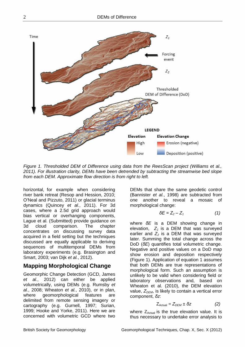
Figure 1. Thresholded DEM of Difference using data from the ReesScan project (Williams et al., 2011). For illustration clarity, DEMs have been detrended by subtracting the streamwise bed slope from each DEM. Approximate flow direction is from right to left.

horizontal, for example when considering river bank retreat (Resop and Hession, 2010; O'Neal and Pizzuto, 2011) or glacial terminus dynamics (Quincey et al., 2011). For 3d cases, where a 2.5d grid approach would bias vertical or overhanging components, Lague et al. (Submitted) provide guidance on 3d cloud comparison. The chapter concentrates on discussing survey data acquired in a field setting but the techniques discussed are equally applicable to deriving sequences of multitemporal DEMs from laboratory experiments (e.g. Brasington and Smart, 2003; van Dijk et al., 2012).

Mapping Morphological Change

Geomorphic Change Detection (GCD, James et al., 2012) can either be applied volumetrically, using DEMs (e.g. Rumsby et al., 2008; Wheaton et al., 2010), or in plan, where geomorphological features are delimited from remote sensing imagery or cartography (e.g. Gurnell, 1997; Surian, 1999; Hooke and Yorke, 2011). Here we are concerned with volumetric GCD where two

DEMs that share the same geodetic control (Bannister et al., 1998) are subtracted from one another to reveal a mosaic of morphological change:

δE = Z2 – Z1 (1)

where δE is a DEM showing change in elevation, Z1 is a DEM that was surveyed earlier and Z2 is a DEM that was surveyed later. Summing the total change across the DoD (δE) quantifies total volumetric change. Negative and positive values on a DoD map show erosion and deposition respectively (Figure 1). Application of equation 1 assumes that both DEMs are true representations of morphological form. Such an assumption is unlikely to be valid when considering field or laboratory observations and, based on Wheaton et al. (2010), the DEM elevation value, ZDEM, is likely to contain a vertical error component, δz:

ZActual = ZDEM ± δz (2)

where ZActual is the true elevation value. It is thus necessary to undertake error analysis to

3 Richard David Williams


ensure that a DoD is reliable. Suitable error analysis techniques are discussed in the “Error Analysis” section below.

Applications

Geomorphology

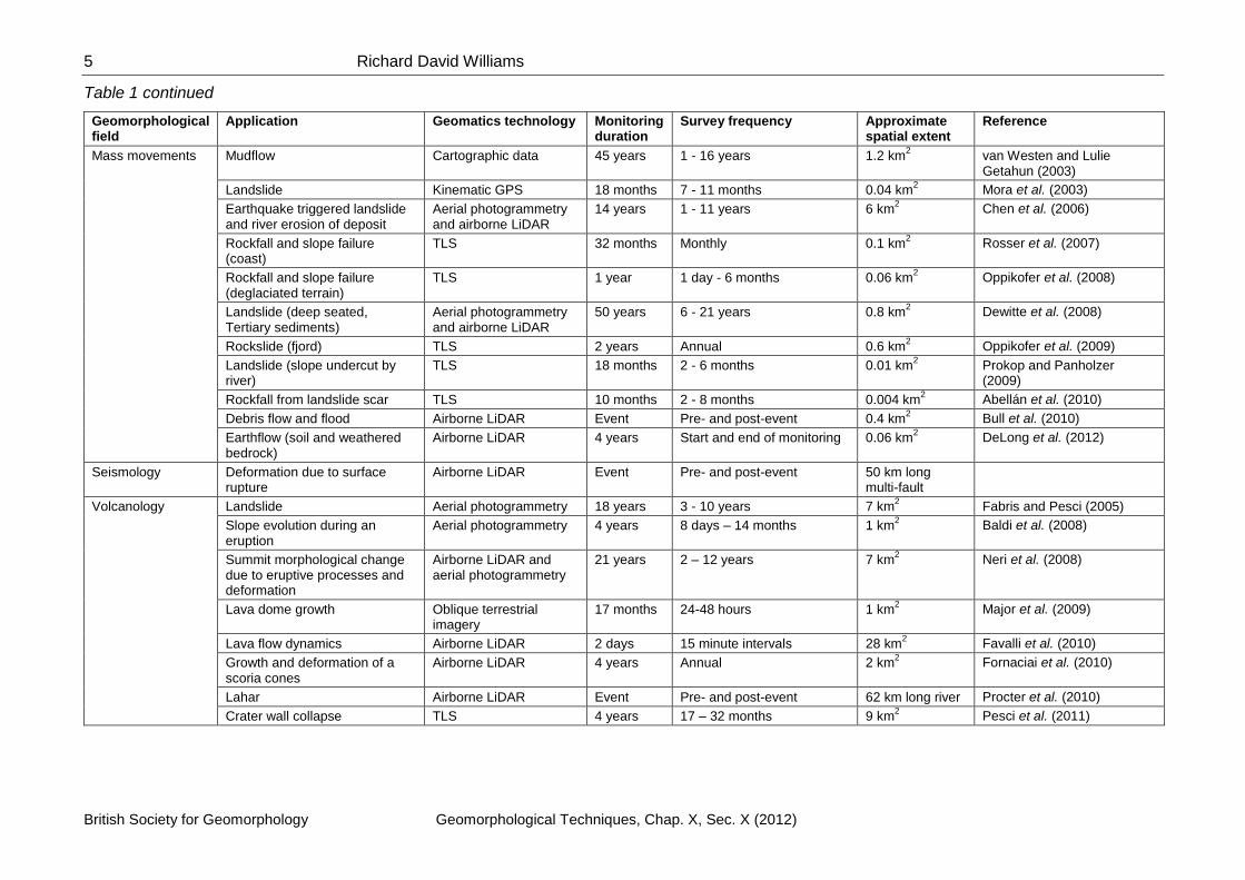
A variety of geomatics technologies and processing techniques have been applied across the geomorphological discipline to quantify volumetric changes at a range of temporal frequencies and spatial extents (Table 1). These have included terrestrial, airborne and spaceborne photogrammetry, terrestrial laser scanning (TLS), airborne Light Detection and Ranging (LiDAR), Real Time Kinematic Global Positioning System (RTK-GPS) and total station survey. In coastal geomorphology sequences of multitemporal DEMs have been used to estimate beach level changes associated with the passage of a hurricane (Zhang et al., 2005), cliff erosion rates during a year-long monitoring period (James and Robson, 2012) and estuarine bathymetric evolution at a 50-year frequency during a 150 year period (van der Wal et al., 2002). DEMs of Difference have also been widely applied to monitor mass movements (Jaboyedoff et al., 2012) where TLS has emerged as the benchmark technology for monitoring rockfalls (e.g. Rosser et al., 2007; Oppikofer et al., 2009). Landslides have been monitored using a range of geomatics technologies (e.g. Mora et al., 2003; Chen et al., 2006), and debris- and earth-flows have been monitored using airborne LiDAR (e.g. Bull et al., 2010; DeLong et al., 2012). Applications of successive DEMs in volcanology also exemplify the range of temporal frequencies and monitoring durations that can be considered. For example, investigations have quantified changes in lava flow fields every 15 minutes during several days (Favalli et al., 2010), lava dome growth every day for over a year (Major et al., 2009), bi-monthly monitoring of slope evolution during effusive eruption (Baldi et al., 2008) and morphostructural change during several decades (Neri et al., 2008). Sequences of multi-temporal DEMs have also been acquired and differenced in glaciology with applications in glacial, proglacial and periglacial settings (e.g. Barrand et al., 2009; Fischer et al., 2011; Carrivick et al., 2012).

Overall, the breadth of examples from across the geomorphological discipline illustrate that

quantitative measures of morphological change provide a principal analysis technique for many investigations that consider change in Earth surface form. In fluvial geomorphology, considerable attention has been focused upon evaluating survey errors because geomorphic change is often only just detectable above the accuracy of the survey technique being applied. In contrast, investigations in other geomorphological fields tend to focus little attention on quantifying errors. In some cases this is justified since the magnitude of geomorphic change is of a far greater magnitude than survey errors. However, in other cases appropriate error analysis would provide a more rigorous estimate of morphological change.Indeed, of all the investigations listed in Table 1, only Favailli et al.’s (2010) investigation of an evolving lava field provides an example of rigorously assessing the reliability of multitemporal DEMs.

Fluvial Geomorphology

DoDs have been widely applied in fluvial geomorphology to (i) infer bedload sediment transport rates; (ii) interpret processes such as channel scour, fill, migration and avulsion; (iii) map the disturbance of ecological habitats; (iv) estimate bed level trends; (v) validate morphological models; and (vi) manage gravel extraction and replenishment schemes. Of these investigation types, the main difference between them is whether their objective is purely to map bed level change or to estimate the rate of bedload sediment transport. Table 2 lists pertinent studies that have applied DoDs in fluvial geomorphology and summarises the survey technologies applied.

Since bedload is the primary determinant of channel morphology (Leopold, 1992; Church, 2006), the morphometric method provides an indirect alternative to the notoriously difficult task of directly sampling and measuring bedload transport rates (Gomez, 1991), so long as the scale of application is sufficiently large (Hicks and Gomez, 2005). Ashmore and Church (1998) provide a salient review of the method, which is based upon a continuity relation for the bedload transport rate:

(3)

where Vo and Vi are volumes of sediment flux out of and into the reach respectively, ρ is porosity, δS is change in storage and δt is



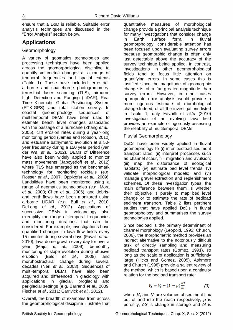
Table 1. Examples of investigations that have applied DEM differencing in a range of geomorphological settings. See Table 2 for a list of fluvial examples.

Geomorphological field

Application Geomatics technology Monitoring duration

Survey frequency Approximate spatial extent

Reference

Coasts Estuary change Bathymetric charts (lead lines and echo sounding)

150 years Half-century 217 km2 van der Wal et al. (2002)

Estuary change induced by earthquakes

Airborne LiDAR 5 months Start and end of monitoring 5 km2 Measures et al. (2011)

Beach changes after a hurricane

Airborne LiDAR Event Pre- and post-event 40 km long coastline

Zhang et al. (2005)

Cliff and gully erosion Airborne LiDAR 6 years Start and end of monitoring 77 km long coastline

Young and Ashford (2006)

Cliff erosion TLS 16 months Monthly 0.1 km2 Rosser et al. (2005)

Cliff erosion TLS 1 year Start and end of monitoring 0.005 km2 Hobbs et al. (2010)

Cliff erosion Oblique terrestrial imagery: SfM and MultiView Stereo

1 year 7 surveys during 1 year 0.05 km long coastline

James et al. (2012)

Fluvial reworking of sediment stores

Talus cone erosion TLS 3 months Start and end of monitoring 0.009 km2 Morche et al. (2008)

Cut / fill of gully and alluvial fan Kinematic GPS 32 months 3 - 5 months 0.5 km2 Fuller and Marden (2010)

Glaciology Glacier surface elevation change

Aerial photogrammetry 1 year Start and end of monitoring 6.3 km2 Hubbard et al. (2000)

Glacier surface elevation change

Aerial photogrammetry and cartographic data

18 years Start and end of monitoring 5.5 km2 Rippin et al. (2003)

Rockglacier movement TLS 8 years 1 month - 3 years 0.04 km2 Avian et al. (2009)


Aerial photogrammetry and airborne LiDAR

2 years Start and end of monitoring 6 km2 Barrand et al. (2009)

Debris covered glacier margins Airborne LiDAR 4 years Start and end of monitoring 0.5 km2 Abermann et al. (2010)

Permafrost affected bedrock and glacier ice


51 years 2 - 22 years 6.5 km2 Fischer et al. (2011)

Forefield sediment redistribution Airborne LiDAR 2 years Start and end of monitoring 2 km2 Irvine-Fynn et al. (2011)

Proglacial and braidplain change

Airborne LiDAR and TLS

2 years 1 day - 1 year 1.5 km2 Carrivick et al. (2012)


TLS 5 days Daily 0.05 km2 Nield et al. (2012)



Table 1 continued

Geomorphological field

Application Geomatics technology Monitoring duration

Survey frequency Approximate spatial extent

Reference

Mass movements Mudflow Cartographic data 45 years 1 - 16 years 1.2 km2 van Westen and Lulie

Getahun (2003)

Landslide Kinematic GPS 18 months 7 - 11 months 0.04 km2 Mora et al. (2003)

Earthquake triggered landslide and river erosion of deposit


14 years 1 - 11 years 6 km2 Chen et al. (2006)

Rockfall and slope failure (coast)

TLS 32 months Monthly 0.1 km2 Rosser et al. (2007)

Rockfall and slope failure (deglaciated terrain)

TLS 1 year 1 day - 6 months 0.06 km2 Oppikofer et al. (2008)

Landslide (deep seated, Tertiary sediments)


50 years 6 - 21 years 0.8 km2 Dewitte et al. (2008)

Rockslide (fjord) TLS 2 years Annual 0.6 km2 Oppikofer et al. (2009)

Landslide (slope undercut by river)

TLS 18 months 2 - 6 months 0.01 km2 Prokop and Panholzer

(2009)

Rockfall from landslide scar TLS 10 months 2 - 8 months 0.004 km2 Abellán et al. (2010)

Debris flow and flood Airborne LiDAR Event Pre- and post-event 0.4 km2 Bull et al. (2010)

Earthflow (soil and weathered bedrock)

Airborne LiDAR 4 years Start and end of monitoring 0.06 km2 DeLong et al. (2012)

Seismology Deformation due to surface rupture

Airborne LiDAR Event Pre- and post-event 50 km long multi-fault

Volcanology Landslide Aerial photogrammetry 18 years 3 - 10 years 7 km2 Fabris and Pesci (2005)

Slope evolution during an eruption

Aerial photogrammetry 4 years 8 days – 14 months 1 km2 Baldi et al. (2008)

Summit morphological change due to eruptive processes and deformation

Airborne LiDAR and aerial photogrammetry

21 years 2 – 12 years 7 km2 Neri et al. (2008)

Lava dome growth Oblique terrestrial imagery

17 months 24-48 hours 1 km2 Major et al. (2009)

Lava flow dynamics Airborne LiDAR 2 days 15 minute intervals 28 km2 Favalli et al. (2010)

Growth and deformation of a scoria cones

Airborne LiDAR 4 years Annual 2 km2 Fornaciai et al. (2010)

Lahar Airborne LiDAR Event Pre- and post-event 62 km long river Procter et al. (2010)

Crater wall collapse TLS 4 years 17 – 32 months 9 km2 Pesci et al. (2011)



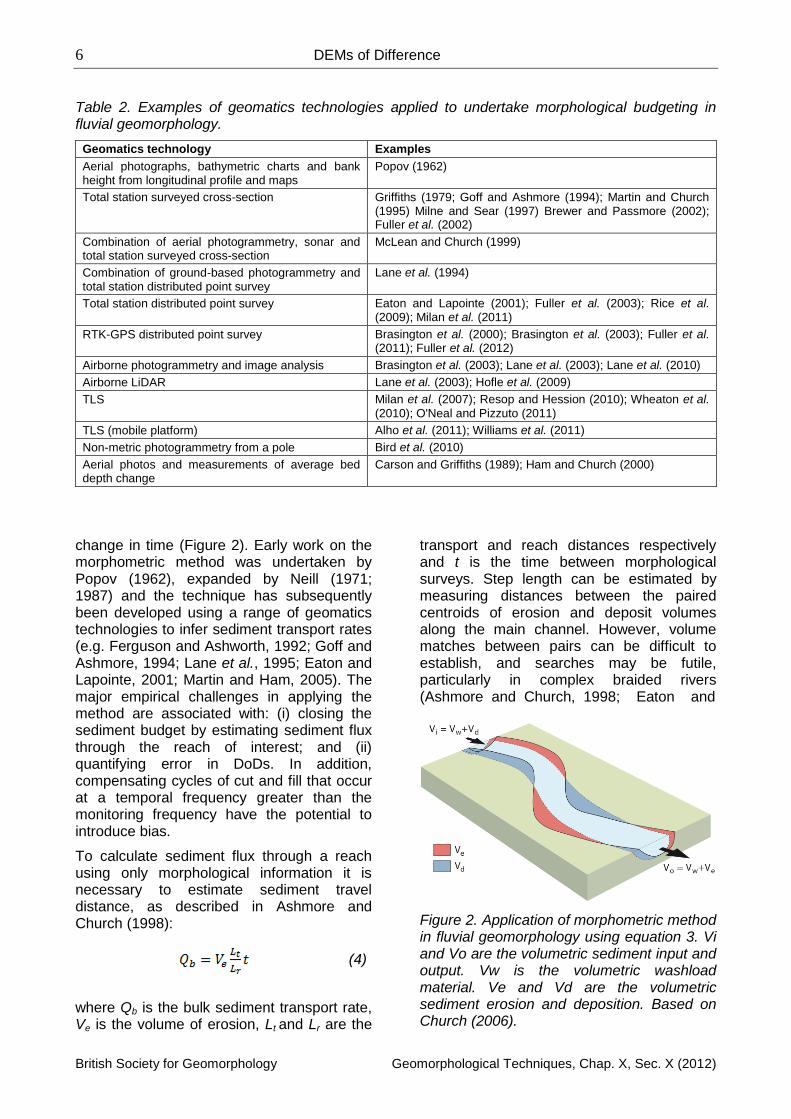
Table 2. Examples of geomatics technologies applied to undertake morphological budgeting in fluvial geomorphology.

Geomatics technology Examples

Aerial photographs, bathymetric charts and bank height from longitudinal profile and maps

Popov (1962)

Total station surveyed cross-section Griffiths (1979; Goff and Ashmore (1994); Martin and Church (1995) Milne and Sear (1997) Brewer and Passmore (2002); Fuller et al. (2002)

Combination of aerial photogrammetry, sonar and total station surveyed cross-section

McLean and Church (1999)

Combination of ground-based photogrammetry and total station distributed point survey

Lane et al. (1994)

Total station distributed point survey Eaton and Lapointe (2001); Fuller et al. (2003); Rice et al. (2009); Milan et al. (2011)

RTK-GPS distributed point survey Brasington et al. (2000); Brasington et al. (2003); Fuller et al. (2011); Fuller et al. (2012)

Airborne photogrammetry and image analysis Brasington et al. (2003); Lane et al. (2003); Lane et al. (2010)

Airborne LiDAR Lane et al. (2003); Hofle et al. (2009)

TLS Milan et al. (2007); Resop and Hession (2010); Wheaton et al.

(2010); O'Neal and Pizzuto (2011)

TLS (mobile platform) Alho et al. (2011); Williams et al. (2011)

Non-metric photogrammetry from a pole Bird et al. (2010)

Aerial photos and measurements of average bed depth change

Carson and Griffiths (1989); Ham and Church (2000)

change in time (Figure 2). Early work on the morphometric method was undertaken by Popov (1962), expanded by Neill (1971; 1987) and the technique has subsequently been developed using a range of geomatics technologies to infer sediment transport rates (e.g. Ferguson and Ashworth, 1992; Goff and Ashmore, 1994; Lane et al., 1995; Eaton and Lapointe, 2001; Martin and Ham, 2005). The major empirical challenges in applying the method are associated with: (i) closing the sediment budget by estimating sediment flux through the reach of interest; and (ii) quantifying error in DoDs. In addition, compensating cycles of cut and fill that occur at a temporal frequency greater than the monitoring frequency have the potential to introduce bias.

To calculate sediment flux through a reach using only morphological information it is necessary to estimate sediment travel distance, as described in Ashmore and Church (1998):

(4)

where Qb is the bulk sediment transport rate, Ve is the volume of erosion, Lt and Lr are the

transport and reach distances respectively and t is the time between morphological surveys. Step length can be estimated by measuring distances between the paired centroids of erosion and deposit volumes along the main channel. However, volume matches between pairs can be difficult to establish, and searches may be futile, particularly in complex braided rivers (Ashmore and Church, 1998; Eaton and

Figure 2. Application of morphometric method in fluvial geomorphology using equation 3. Vi and Vo are the volumetric sediment input and output. Vw is the volumetric washload material. Ve and Vd are the volumetric sediment erosion and deposition. Based on Church (2006).



Lapointe, 2001). Alternatives approaches to estimating sediment flux through the reach of interest include bedload sampling (Lane et al., 1995), and using tracer pebbles to estimate travel distances and sediment mobility patterns (Schwendel et al., 2010).

The advent of remote sensing techniques enables spatially continuous surveys of topography and has largely replaced the prism based method of interpolating cross-sections in a streamwise direction to estimate volumetric change (Griffiths, 1979; Ferguson and Ashworth, 1992; Martin and Church, 1995) or techniques to estimate the aerial extent of bed material depth changes from aerial photos (Ham and Church, 2000). In some situations, however, survey by regular cross-sections remains the primary means of monitoring channel morphology for long-term (annual to decadal) sediment budgeting. Indeed, many unitary authorities commission cross-section surveys to monitor channel topography due to the cost-effective nature of this survey technique. Discussions on the balance between cross-section spacing and accuracy in morphological budgeting can be found in Lane et al. (2003), Hicks (2012) and Lindsay and Ashmore (2002).

Error Analysis

DEMs are unlikely to be exact representations of the Earth’s surface due to a variety of uncertainties including those

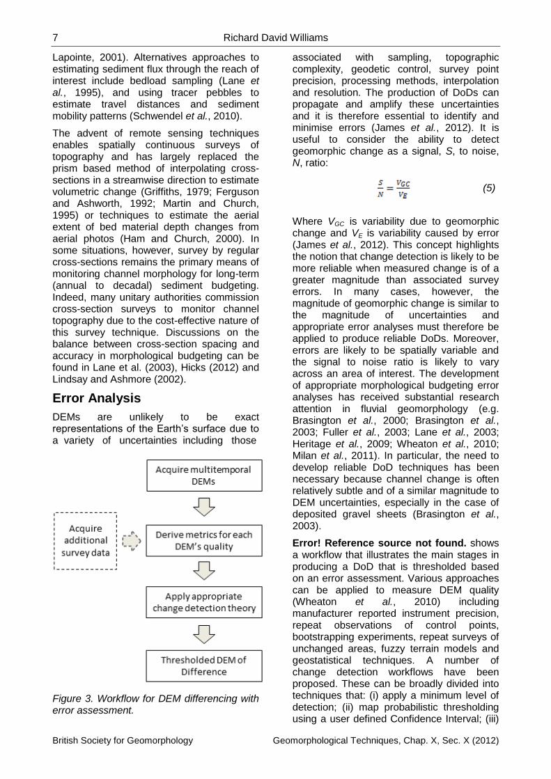
Figure 3. Workflow for DEM differencing with error assessment.

associated with sampling, topographic complexity, geodetic control, survey point precision, processing methods, interpolation and resolution. The production of DoDs can propagate and amplify these uncertainties and it is therefore essential to identify and minimise errors (James et al., 2012). It is useful to consider the ability to detect geomorphic change as a signal, S, to noise, N, ratio:

(5)

Where VGC is variability due to geomorphic change and VE is variability caused by error (James et al., 2012). This concept highlights the notion that change detection is likely to be more reliable when measured change is of a greater magnitude than associated survey errors. In many cases, however, the magnitude of geomorphic change is similar to the magnitude of uncertainties and appropriate error analyses must therefore be applied to produce reliable DoDs. Moreover, errors are likely to be spatially variable and the signal to noise ratio is likely to vary across an area of interest. The development of appropriate morphological budgeting error analyses has received substantial research attention in fluvial geomorphology (e.g. Brasington et al., 2000; Brasington et al., 2003; Fuller et al., 2003; Lane et al., 2003; Heritage et al., 2009; Wheaton et al., 2010; Milan et al., 2011). In particular, the need to develop reliable DoD techniques has been necessary because channel change is often relatively subtle and of a similar magnitude to DEM uncertainties, especially in the case of deposited gravel sheets (Brasington et al., 2003).

Error! Reference source not found. shows a workflow that illustrates the main stages in producing a DoD that is thresholded based on an error assessment. Various approaches can be applied to measure DEM quality (Wheaton et al., 2010) including manufacturer reported instrument precision, repeat observations of control points, bootstrapping experiments, repeat surveys of unchanged areas, fuzzy terrain models and geostatistical techniques. A number of change detection workflows have been proposed. These can be broadly divided into techniques that: (i) apply a minimum level of detection; (ii) map probabilistic thresholding using a user defined Confidence Interval; (iii)



consider the spatial variability of uncertainty from multiple parameters; and (iv) assess the spatial coherence of erosion and deposition. Each of these techniques is summarised below, and the associated advantages and disadvantages of each approach are discussed.

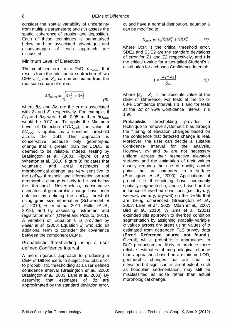
Minimum Level of Detection

The combined error in a DoD, δUDOD, that results from the addition or subtraction of two DEMs, Z1 and Z2, can be estimated from the root sum square of errors:

(6)

where δz1 and δz2 are the errors associated with Z1 and Z2 respectively. For example, if δz1 and δz2 were both 0.05 m then δUDOD would be 0.07 m. To apply the Minimum Level of Detection (LODMin), the value of δUDOD is applied as a constant threshold across the DoD. This approach is conservative because only geomorphic change that is greater than the LODMin is deemed to be reliable. Indeed, testing by Brasington et al. (2003: Figure 8) and Wheaton et al. (2010: Figure 3) indicates that volumetric and areal estimates of morphological change are very sensitive to the LoDMin threshold and information on real geomorphic change is likely to be lost below the threshold. Nevertheless, conservative estimates of geomorphic change have been obtained by defining the LoDMin threshold using grain size information (Schwendel et al., 2010; Fuller et al., 2011; Fuller et al., 2012), and by assessing instrument and registration error (O'Neal and Pizzuto, 2011). A variation on Equation 6 is provided by Fuller et al. (2003: Equation 6) who add an additional term to consider the covariance between the component DEMs.

Probabilistic thresholding using a user defined Confidence Interval

A more rigorous approach to producing a DEM of Difference is to subject the total error to probabilistic thresholding at a user defined confidence interval (Brasington et al., 2000; Brasington et al., 2003; Lane et al., 2003). By assuming that estimates of δz are approximated by the standard deviation error,

σ, and have a normal distribution, equation 6 can be modified to:

(7)

where Ucrit is the critical threshold error, SDE1 and SDE2 are the standard deviations of error for Z1 and Z2 respectively, and t is the critical t-value for a two-tailed Student’s t-distribution for a chosen Confidence Interval:

t = (8)

where |Z2 – Z1| is the absolute value of the DEM of Difference. For tests at the 1σ or 68% Confidence Interval, t ≥ 1 and for tests at the 2σ or 95% Confidence Interval, t ≥ 1.96.

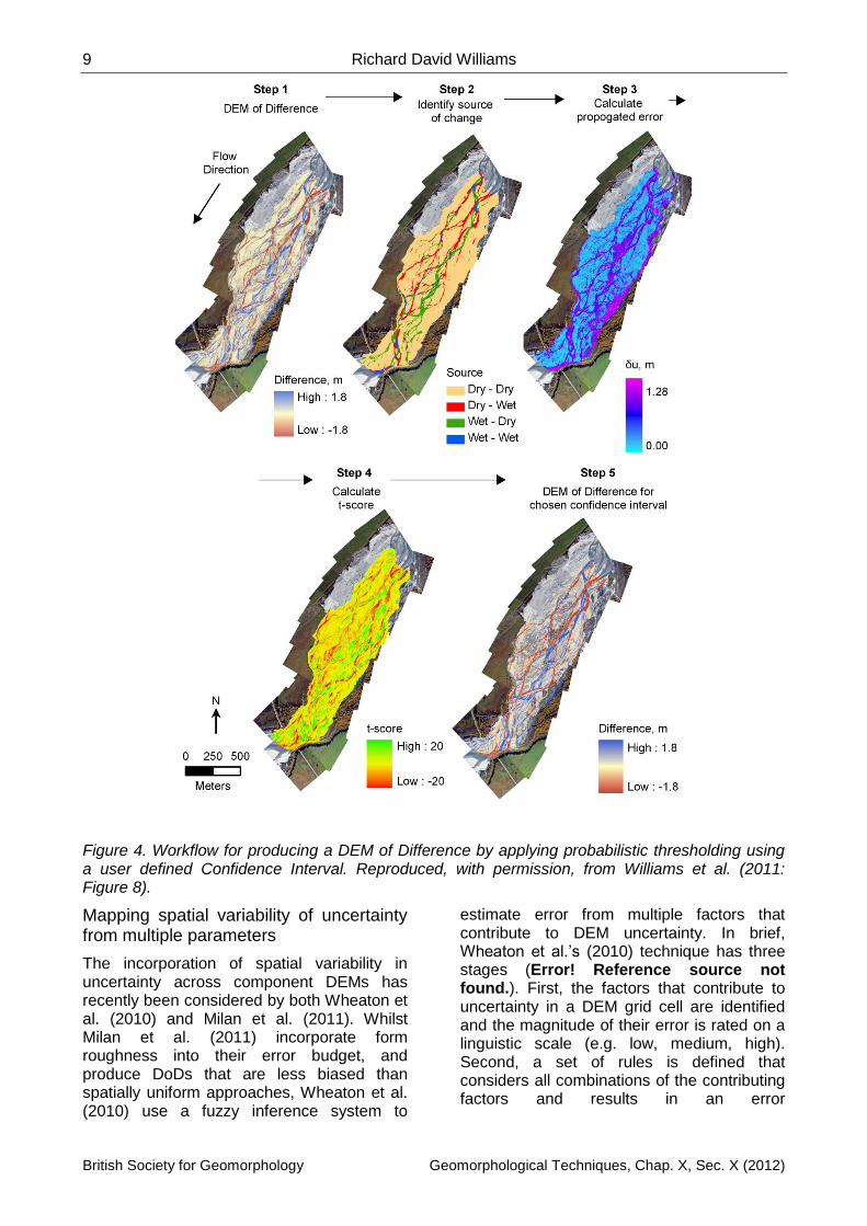
Probabilistic thresholding provides a technique to remove systematic bias through the filtering of elevation changes based on the confidence that detected change is real. Moreover, the user can decide a suitable Confidence Interval for the analysis. However, σ1 and σ2 are not necessary uniform across their respective elevation surfaces and the estimation of their values usually requires the use of quality control points that are compared to a surface (Brasington et al., 2000). Applications of probabilistic thresholding have commonly spatially segmented σ1 and σ2 based on the influence of riverbed conditions (i.e. dry-dry, wet-wet, wet-dry, dry-wet) on the DEMs that are being differenced (Brasington et al., 2003; Lane et al., 2003; Milan et al., 2007; Bird et al., 2010). Williams et al. (2011) extended this approach to riverbed condition segmentation by assigning spatially variable σ values across dry areas using values of σ estimated from detrended TLS survey data (Error! Reference source not found.). Overall, whilst probabilistic approaches to DoD production are likely to produce more reliable estimates of morphological change than approaches based on a minimum LOD, geomorphic changes that are small in elevation but significant in areal extent, such as floodplain sedimentation, may still be misclassified as noise rather than actual morphological change.



Figure 4. Workflow for producing a DEM of Difference by applying probabilistic thresholding using a user defined Confidence Interval. Reproduced, with permission, from Williams et al. (2011: Figure 8).

Mapping spatial variability of uncertainty from multiple parameters

The incorporation of spatial variability in uncertainty across component DEMs has recently been considered by both Wheaton et al. (2010) and Milan et al. (2011). Whilst Milan et al. (2011) incorporate form roughness into their error budget, and produce DoDs that are less biased than spatially uniform approaches, Wheaton et al. (2010) use a fuzzy inference system to

estimate error from multiple factors that contribute to DEM uncertainty. In brief, Wheaton et al.’s (2010) technique has three stages (Error! Reference source not found.). First, the factors that contribute to uncertainty in a DEM grid cell are identified and the magnitude of their error is rated on a linguistic scale (e.g. low, medium, high). Second, a set of rules is defined that considers all combinations of the contributing factors and results in an error



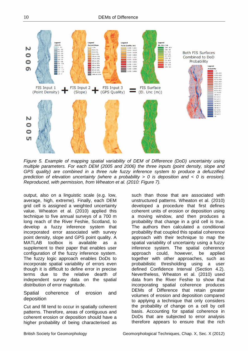
Figure 5. Example of mapping spatial variability of DEM of Difference (DoD) uncertainty using multiple parameters. For each DEM (2005 and 2006) the three inputs (point density, slope and GPS quality) are combined in a three rule fuzzy inference system to produce a defuzzified prediction of elevation uncertainty (where a probability > 0 is deposition and < 0 is erosion). Reproduced, with permission, from Wheaton et al. (2010: Figure 7).

output, also on a linguistic scale (e.g. low, average, high, extreme). Finally, each DEM grid cell is assigned a weighted uncertainty value. Wheaton et al. (2010) applied this technique to five annual surveys of a 700 m long reach of the River Feshie, Scotland, to develop a fuzzy inference system that incorporated error associated with survey point density, slope and GPS point quality. A MATLAB toolbox is available as a supplement to their paper that enables user configuration of the fuzzy inference system. The fuzzy logic approach enables DoDs to incorporate spatial variability of errors even though it is difficult to define error in precise terms due to the relative dearth of independent survey data on the spatial distribution of error magnitude.

Spatial coherence of erosion and deposition

Cut and fill tend to occur in spatially coherent patterns. Therefore, areas of contiguous and coherent erosion or deposition should have a higher probability of being characterised as

such than those that are associated with unstructured patterns. Wheaton et al. (2010) developed a procedure that first defines coherent units of erosion or deposition using a moving window, and then produces a probability that change in a grid cell is true. The authors then calculated a conditional probability that coupled this spatial coherence approach with their technique to map the spatial variability of uncertainty using a fuzzy inference system. The spatial coherence approach could, however, be applied together with other approaches, such as probabilistic thresholding using a user defined Confidence Interval (Section 4.2). Nevertheless, Wheaton et al. (2010) used data from the River Feshie to show that incorporating spatial coherence produces DEMs of Difference that retain greater volumes of erosion and deposition compared to applying a technique that only considers the probability of change on a cell by cell basis. Accounting for spatial coherence in DoDs that are subjected to error analysis therefore appears to ensure that the rich



detail of real geomorphic change is preserved.

Guidance

DEM acquisition and quality

The most important factor for determining the reliability of a DoD is the accuracy of the individual DEMs and their coregistration. The largest errors in DoDs arise in areas with high form and surface roughness, and sparse survey point densities. Therefore the most expedient way to improve the reliability of erosion and deposition estimates is to acquire DEMs that are characterised by levels of precision and accuracy that are commensurate with the magnitude of errors that are acceptable. An investigation’s objectives will, of course, also determine the survey frequency and spatial extent that is necessary and these too will impact detection accuracy. The application of novel remote sensing methodologies, such as Structure from Motion (James and Robson, 2012; Westoby et al., in press) and TLS (Heritage and Hetherington, 2007; Williams et al., 2011) are enabling increasingly rich and dense point cloud datasets to be generated at a relatively low cost. However, filtering and classifying dense datasets to generate a DEM is not necessarily straightforward and requires the use of suitable processing techniques (e.g. Brasington et al., 2012; Brodu and Lague, 2012; Rychkov et al., 2012). Moreover, awareness of appropriate DEM generation techniques is integral to producing high quality DEMs (Heritage et al., 2009; Schwendel et al., 2012). Since other chapters in this volume describe key principles and practices associated with various geomatics technologies that are utilised to produce DEMs, further discussion on minimising survey errors is not warranted here. However, it is pertinent to note that any investigation that intends to acquire survey data for generating DEMs should include consideration of how DEM quality will be measured. This is particularly important when different survey techniques are fused together. For example, in fluvial geomorphology the wetted channel problem (Hicks, 2012) usually requires different geomatics technologies to map exposed and inundated areas of the riverbed (e.g. Brasington and Smart, 2003; Westaway et al., 2003; Williams et al., 2011; Legleiter, 2012).

Software

DoDs can be produced using a variety of Geographic Information System (GIS) and programming software (e.g. Golden Software Surfer, ESRI ArcGIS, Mathworks MATLAB). A very useful utility for ArcGIS is the Geomorphic Change Detection Toolbox (http://gcd.joewheaton.org/home). This Toolbox includes procedures to prepare data, undertake change detection using various uncertainty methods, perform batch runs and segment DoDs. Results are output in a variety of forms including GIS grid files, charts and text files. Help on using the Toolbox is available through a series of online video tutorials and help forums. Whilst users should be aware of the principles associated with geomorphic change detection theory before using automated toolboxes, such software reduces the time required to produce DoDs and thus enables attention to be focused upon interpretation of estimated morphological changes.

Error analysis

The development of appropriate error analyses for DoDs has primarily been undertaken within the field of fluvial geomorphology. This interest has been driven by desire to reliably estimate relatively small magnitudes of geomorphic change relative to uncertainty when applying morphological sediment budgeting in gravel-bed river environments. The techniques developed within fluvial geomorphology are, however, transferable to other geomorphological fields. Indeed, applying appropriate error analyses should be de rigueur for reliably estimating morphological change across all fields of geomorphological enquiry.

Limitations

A range of geomatics technologies enable the acquisition of precise topographic data during repeat surveys. However, the accuracy of a volumetric estimate of morphological change is limited by the temporal frequency of the successive surveys. For example, in fluvial geomorphology, increasing the temporal interval between two surveys is likely to increase the probability that a DoD will incorporate compensating cycles of scour and fill. This is particularly likely if more than one competent flow event has occurred



during the intervening period. The DoD technique thus provides a lower-bound estimate of volumetric change. Ultimately, the utility of a volumetric estimate of change will depend upon the history of forcing events and the characteristics of the environmental setting that is being examined.

Acknowledgements

This chapter was written whilst RDW was in receipt of an Aberystwyth University Postgraduate Research Studentship. Dr Stephen Tooth is thanked for providing comments on an early draft. Comments from two anonymous reviewers also improved the chapter.

References

Abellán A, Calvet J, Vilaplana JM, Blanchard J. 2010. Detection and spatial prediction of rockfalls by means of terrestrial laser scanner monitoring. Geomorphology, 119: 162-171. DOI: 10.1016/j.geomorph.2010.03.016

Abermann J, Fischer A, Lambrecht A, Geist T. 2010. On the potential of very high-resolution repeat DEMs in glacial and periglacial environments. Cryosphere, 4: 53-65. DOI: doi:10.5194/tc-4-53-2010

Alho P, Vaaja M, Kukko A, Kasvi E, Kurkela M, Hyyppa J, Hyyppa H, Kaartinen H. 2011. Mobile laser scanning in fluvial geomorphology: mapping and change detection of point bars. Zeitschrift Fur Geomorphologie, 55: 31-50. DOI: 10.1127/0372-8854/2011/0055s2-0044

Ashmore PE, Church MA. 1998. Sediment transport and river morphology: a paradigm for study. In Gravel Bed Rivers in the Environment, Klingeman PC, Beschta RL, Komar BD, Bradley JB (eds). Water Resources Publications: Oregon; 115-139.

Avian M, Kellerer-Pirklbauer A, Bauer A. 2009. LiDAR for monitoring mass movements in permafrost environments at the cirque Hinteres Langtal, Austria, between 2000 and 2008. Natural Hazards and Earth Systems Science, 9: 1087-1094. DOI: 10.5194/nhess-9-1087-2009

Baldi P, Coltelli M, Fabris M, Marsella M, Tommasi P. 2008. High precision photogrammetry for monitoring the evolution of the NW flank of Stromboli volcano during and after the 2002-2003 eruption. Bulletin of

Volcanology, 70: 703-715. DOI: 10.1007/s00445-007-0162-1

Bannister A, Raymond S, Baker R. 1998. Surveying, Prentice Hall: New Jersey.

Barrand NE, Murray T, James TD, Barr SL, Mills JP. 2009. Optimizing photogrammetric DEMs for glacier volume change assessment using laser-scanning derived ground-control points. Journal of Glaciology, 55: 106-116. DOI: 10.3189/002214309788609001

Bird S, Hogan D, Schwab J. 2010. Photogrammetric monitoring of small streams under a riparian forest canopy. Earth Surface Processes and Landforms, 35: 952-970. DOI: 10.1002/esp.2001

Brasington J, Rumsby BT, Mcvey RA. 2000. Monitoring and modelling morphological change in a braided gravel-bed river using high resolution GPS-based survey. Earth Surface Processes and Landforms, 25: 973-990. DOI: 10.1002/1096-9837(200008)25:9<973::AID-ESP111>3.0.CO;2-Y

Brasington J, Langham J, Rumsby B. 2003. Methodological sensitivity of morphometric estimates of coarse fluvial sediment transport. Geomorphology, 53: 299-316. DOI: 10.1016/S0169-555X(02)00320-3

Brasington J, Smart RMA. 2003. Close range digital photogrammetric analysis of experimental drainage basin evolution. Earth Surface Processes and Landforms, 28: 231-247. DOI: 10.1002/esp.480

Brasington J, Vericat D, Rychkov I. 2012. Modelling river bed morphology, roughness and surface sedimentology using high resolution terrestrial laser scanning. Water Resources Research, 48: W11519. DOI: 10.1029/2012WR012223

Brewer PA, Passmore DG. 2002. Sediment budgeting techniques in gravel-bed rivers. In Sediment Flux to Basins: Causes, Controls and Consequences, Jones SJ, Frostick LE (eds). Geology Society: London; 97-113. DOI: 10.1144/GSL.SP.2002.191.01.07

Brodu N, Lague D. 2012. 3D terrestrial lidar data classification of complex natural scenes using a multi-scale dimensionality criterion: Applications in geomorphology. ISPRS Journal of Photogrammetry and Remote Sensing, 68: 121-134. DOI: 10.1016/j.isprsjprs.2012.01.006



Bull JM, Miller H, Gravley DM, Costello D, Hikuroa DCH, Dix JK. 2010. Assessing debris flows using LIDAR differencing: 18 May 2005 Matata event, New Zealand. Geomorphology, 124: 75-84. DOI: 10.1016/j.geomorph.2010.08.011

Carrivick JL, Geilhausen M, Warburton J, Dickson NE, Carver SJ, Evans AJ, Brown LE. 2012. Contemporary geomorphological activity throughout the proglacial area of an alpine catchment. Geomorphology. DOI: 10.1016/j.geomorph.2012.03.029

Carson MA, Griffiths GA. 1989. Gravel transport in the braided Waimakariri River - mechanisms, measurements and predictions. Journal of Hydrology, 109: 201-220. DOI: 10.1016/0022-1694(89)90016-4,

Chen R-F, Chang K-J, Angelier J, Chan Y-C, Deffontaines B, Lee C-T, Lin M-L. 2006. Topographical changes revealed by high-resolution airborne LiDAR data: The 1999 Tsaoling landslide induced by the Chi–Chi earthquake. Engineering Geology, 88: 160-172. DOI: 10.1016/j.enggeo.2006.09.008

Church M. 2006. Bed material transport and the morphology of alluvial river channels. Annual Review of Earth and Planetary Sciences, 34: 325-354. DOI: 10.1146/annurev.earth.33.092203.122721

Delong SB, Prentice CS, Hilley GE, Ebert Y. 2012. Multitemporal ALSM change detection, sediment delivery, and process mapping at an active earthflow. Earth Surface Processes and Landforms, 37: 262-272. DOI: 10.1002/esp.2234

Dewitte O, Jasselette JC, Cornet Y, Van Den Eeckhaut M, Collignon A, Poesen J, Demoulin A. 2008. Tracking landslide displacements by multi-temporal DTMs: A combined aerial stereophotogrammetric and LIDAR approach in western Belgium. Engineering Geology, 99: 11-22. DOI: 10.1016/j.enggeo.2008.02.006

Eaton BC, Lapointe MF. 2001. Effects of large floods on sediment transport and reach morphology in the cobble-bed Sainte Marguerite River. Geomorphology, 40: 291-309. DOI: 10.1016/s0169-555x(01)00056-3

Fabris M, Pesci A. 2005. Automated DEM extraction in digital aerial photogrammetry: precision and validation for mass movement monitoring. Annals of Geophysics, 48: 973-988. DOI: 10.4401/ag-3247

Favalli M, Fornaciai A, Mazzarini F, Harris A, Neri M, Behncke B, Pareschi MT, Tarquini S, Boschi E. 2010. Evolution of an active lava flow field using a multitemporal LIDAR acquisition. Journal of Geophysical Research-Solid Earth, 115: B11203. DOI: 10.1029/2010jb007463

Ferguson R, Ashworth PJ. 1992. Spatial patterns of bedload transport and channel change in braided and near-braided rivers. In Dynamics of Gravel-bed Rivers, Billi P, Hey RD, Thorne CR, Tacconi P (eds). John Wiley & Sons Ltd; 477-492.

Fischer L, Eisenbeiss H, Kääb A, Huggel C, Haeberli W. 2011. Monitoring topographic changes in a periglacial high-mountain face using high-resolution DTMs, Monte Rosa East Face, Italian Alps. Permafrost and Periglacial Processes, 22: 140-152. DOI: 10.1002/ppp.717

Fornaciai A, Behncke B, Favalli M, Neri M, Tarquini S, Boschi E. 2010. Detecting short-term evolution of Etnean scoria cones: a LIDAR-based approach. Bulletin of Volcanology, 72: 1209-1222. DOI: 10.1007/s00445-010-0394-3

Fuller IC, Passmore DG, Heritage GL, Large ARG, Brewer PA. 2002. Annual sediment budgets in an unstable gravel-bed river: the River Coquet, northern England. In Sediment Flux to Basins: Causes, Controls and Consequences, Jones SJ, Frostick LE (eds). Geology Society: London; 115-131.

Fuller IC, Large ARG, Charlton ME, Heritage GL, Milan DJ. 2003. Reach-scale sediment transfers: an evaluation of two morphological budgeting approaches. Earth Surface Processes and Landforms, 28: 889-903. DOI: 10.1002/esp.1011

Fuller IC, Marden M. 2010. Rapid channel response to variability in sediment supply: Cutting and filling of the Tarndale Fan, Waipaoa catchment, New Zealand. Marine Geology, 270: 45-54. DOI: 10.1016/j.margeo.2009.10.004

Fuller IC, Basher L, Marden M, Massey C. 2011. Using Morphological Adjustments to Appraise Sediment Flux. Journal of Hydrology (New Zealand), 50: 59-79. DOI: 10.1144/GSL.SP.2002.191.01.08

Fuller IC, Richardson JM, Basher L, Dykes RC, Vale SS. 2012. Responses to river management? Geomorphic change over



decadal and annual timescales in two gravel-bed rivers in New Zealand. In River Channels: Types, Dynamics and Changes, Molina D (ed). Nova Science: New York; 137-163.

Goff JR, Ashmore P. 1994. Gravel transport and morphological change in braided Sunwapta River, Alberta, Canada. Earth Surface Processes and Landforms, 19: 195-212. DOI: 10.1002/esp.3290190302

Gomez B. 1991. Bedload transport. Earth-Science Reviews, 31: 89-132. DOI: 10.1016/0012-8252(91)90017-a

Griffiths GA. 1979. Recent sedimentation history of the Waimakariri River, New Zealand. Journal of Hydrology (New Zealand), 18: 6-28.

Gurnell AM. 1997. Channel change on the River Dee meanders, 1946–1992, from the analysis of air photographs. Regulated Rivers: Research & Management, 13: 13-26.

Ham DG, Church M. 2000. Bed-material transport estimated from channel morphodynamics: Chilliwack River, British Columbia. Earth Surface Processes and Landforms, 25: 1123-1142. DOI: 10.1002/1096-9837(200009)25:10<1123::AID-ESP122>3.0.CO;2-9

Heritage GL, Hetherington DJ. 2007. Towards a protocol for laser scanning in fluvial geomorphology. Earth Surface Processes and Landforms, 32: 66-74. DOI: 10.1002/esp.1375

Heritage GL, Milan DJ, Large ARG, Fuller IC. 2009. Influence of survey strategy and interpolation model on DEM quality. Geomorphology, 112: 334-344. DOI: 10.1016/j.geomorph.2009.06.024

Hicks DM, Gomez B. 2005. Sediment Transport. In Tools in Fluvial Geomorphology, Kondolf GM, Piegay H (eds). Wiley: Chichester, England; 425-461. DOI: 10.1002/0470868333.ch15

Hicks DM. 2012. Remotely Sensed Topographic Change in Gravel Riverbeds with Flowing Channels. In Gravel-Bed Rivers. Wiley; 303-314. DOI: 10.1002/9781119952497.ch23

Hobbs PRN, Gibson A, Jones L, Pennington C, Jenkins G, Pearson S, Freeborough K. 2010. Monitoring coastal change using

terrestrial LiDAR. Geological Society, London, Special Publications, 345: 117-127. DOI: 10.1144/sp345.12

Hofle B, Vetter M, Pfeifer N, Mandlburger G, Stotter J. 2009. Water surface mapping from airborne laser scanning using signal intensity and elevation data. Earth Surface Processes and Landforms, 34: 1635-1649. DOI: 10.1002/esp.1853

Hooke JM, Yorke L. 2011. Channel bar dynamics on multi-decadal timescales in an active meandering river. Earth Surface Processes and Landforms, 36: 1910-1928. DOI: 10.1002/esp.2214

Hubbard A, Willis I, Sharp M, Mair D, Nienow P, Hubbard B, Blatter H. 2000. Glacier mass-balance determination by remote sensing and high-resolution modelling. Journal of Glaciology, 46: 491-498. DOI: 10.3189/172756500781833016

Irvine-Fynn TDL, Barrand NE, Porter PR, Hodson AJ, Murray T. 2011. Recent High-Arctic glacial sediment redistribution: A process perspective using airborne lidar. Geomorphology, 125: 27-39. DOI: 10.1016/j.geomorph.2010.08.012

Jaboyedoff M, Oppikofer T, Abellán A, Derron M-H, Loye A, Metzger R, Pedrazzini A. 2012. Use of LIDAR in landslide investigations: a review. Natural Hazards, 61: 5-28. DOI: 10.1007/s11069-010-9634-2

James LA, Hodgson ME, Ghoshal S, Latiolais MM. 2012. Geomorphic change detection using historic maps and DEM differencing: The temporal dimension of geospatial analysis. Geomorphology, 137: 181-198. DOI: 10.1016/j.geomorph.2010.10.039

James MR, Robson S. 2012. Straightforward reconstruction of 3D surfaces and topography with a camera: Accuracy and geoscience application. J. Geophys. Res., 117: F03017. DOI: 10.1029/2011jf002289

Lague D, Brodu N, Leroux J. Submitted. A new method for high precision 3D deformation measurement of complex topography with terrestrial laser scanner: application to the Rangitikei canyon (N-Z). ISPRS Journal of Photogrammetry and Remote Sensing.

Lane SN, Chandler JH, Richards KS. 1994. Developments in monitoring and modelling small-scale river bed topography. Earth



Surface Processes and Landforms, 19: 349-368. DOI: 10.1002/esp.3290190406

Lane SN, Richards K, Chandler J. 1995. Morphological estimation of the time-integrated bed load transport rate. Water Resources Research, 31: 761-772. DOI: 10.1029/94WR01726

Lane SN, Westaway RM, Hicks DM. 2003. Estimation of erosion and deposition volumes in a large, gravel-bed, braided river using synoptic remote sensing. Earth Surface Processes and Landforms, 28: 249-271. DOI: 10.1002/esp.483

Lane SN, Widdison PE, Thomas RE, Ashworth PJ, Best JL, Lunt IA, Smith GHS, Simpson CJ. 2010. Quantification of braided river channel change using archival digital image analysis. Earth Surface Processes and Landforms, 35: 971-985. DOI: 10.1002/esp.2015

Legleiter CJ. 2012. Remote measurement of river morphology via fusion of LiDAR topography and spectrally based bathymetry. Earth Surface Processes and Landforms, 37: 499-518. DOI: 10.1002/esp.2262

Leopold LB. 1992. Sediment size that determines channel geometry. In Dynamics of Gravel-Bed Rivers, Billi P, Hey RD, Thorne CR, Tacconi P (eds). Wiley: Chichester; 297-311.

Lindsay JB, Ashmore PE. 2002. The effects of survey frequency on estimates of scour and fill in a braided river model. Earth Surface Processes and Landforms, 27: 27-43. DOI: 10.1002/esp.282

Major JJ, Dzurisin D, Schilling SP, Poland MP. 2009. Monitoring lava-dome growth during the 2004-2008 Mount St. Helens, Washington, eruption using oblique terrestrial photography. Earth and Planetary Science Letters, 286: 243-254. DOI: 10.1016/j.epsl.2009.06.034

Martin Y, Church M. 1995. Bed-material transport estimated from channel surveys: Vedder River, British Columbia. Earth Surface Processes and Landforms, 20: 347-361. DOI: 10.1002/esp.3290200405

Martin Y, Ham D. 2005. Testing bedload transport formulae using morphologic transport estimates and field data: lower Fraser River, British Columbia. Earth Surface Processes and Landforms, 30: 1265-1282. DOI: 10.1002/esp.1200

Mclean DG, Church M. 1999. Sediment transport along lower Fraser River: 2. Estimates based on the long-term gravel budget. Water Resources Research, 35: 2549-2559. DOI: 10.1029/1999wr900102

Measures R, Hicks DM, Shankar U, Bind J, Arnold J, Zeldis J. 2011. Mapping earthquake induced topographical change and liquefaction in the Avon-Heathcote Estuary, Environment Canterbury Regional Council: Christchurch, New Zealand, 32.

Milan DJ, Heritage GL, Hetherington D. 2007. Application of a 3D laser scanner in the assessment of erosion and deposition volumes and channel change in a proglacial river. Earth Surface Processes and Landforms, 32: 1657-1674. DOI: 10.1002/esp.1592

Milan DJ, Heritage GL, Large ARG, Fuller IC. 2011. Filtering spatial error from DEMs: Implications for morphological change estimation. Geomorphology, 125: 160-171. DOI: 10.1016/j.geomorph.2010.09.012

Milne JA, Sear DA. 1997. Modelling river channel topography using GIS. International Journal of Geographical Information Science, 11: 499-519. DOI: 10.1080/136588197242275

Mora P, Baldi P, Casula G, Fabris M, Ghirotti M, Mazzini E, Pesci A. 2003. Global Positioning Systems and digital photogrammetry for the monitoring of mass movements: application to the Ca' di Malta landslide (northern Apennines, Italy). Engineering Geology, 68: 103-121. DOI: 10.1016/s0013-7952(02)00200-4

Morche D, Schmidt K-H, Sahling I, Herkommer M, Kutschera J. 2008. Volume changes of Alpine sediment stores in a state of post-event disequilibrium and the implications for downstream hydrology and bed load transport. Norwegian Journal of Geography, 62: 89-101. DOI: 10.1080/00291950802095079

Mukoyama S. 2011. Estimation of ground deformation caused by the earthquake (M7.2) in Japan, 2008, from the geomorphic image analysis of high resolution LiDAR DEMs. Journal of Mountain Science, 8: 239-245. DOI: 10.1007/s11629-011-2106-7

Neill CR. 1971. River bed transport related to meander migration rates. Journal of Waterways, Habors and Coastal Engineering,



American Society of Civil Engineers, 97: 783-786.

Neill CR. 1987. Sediment balance considerations linking long-term transport and channel processes. In Sediment transport in gravel bed rivers, Thorne CR, Bathurst JC, Hey RD (eds). John Wiley & Sons: Chichester; 225-240.

Neri M, Mazzarini F, Tarquini S, Bisson M, Isola I, Behncke B, Pareschi MT. 2008. The changing face of Mount Etna's summit area documented with Lidar technology. Geophysical Research Letters, 35: L09305. DOI: 10.1029/2008gl033740

Nield JM, Chiverrell RC, Darby SE, Leyland J, Vircavs LH, Jacobs B. 2012. Complex spatial feedbacks of tephra redistribution, ice melt and surface roughness modulate ablation on tephra covered glaciers. Earth Surface Processes and Landforms. DOI: 10.1002/esp.3352

O'neal MA, Pizzuto JE. 2011. The rates and spatial patterns of annual riverbank erosion revealed through terrestrial laser-scanner surveys of the South River, Virginia. Earth Surface Processes and Landforms, 36: 695-701. DOI: 10.1002/esp.2098

Oppikofer T, Jaboyedoff M, Keusen H-R. 2008. Collapse at the eastern Eiger flank in the Swiss Alps. Nature Geoscience, 1: 531-535. DOI: 10.1038/ngeo258

Oppikofer T, Jaboyedoff M, Blikra L, Derron MH, Metzger R. 2009. Characterization and monitoring of the Åknes rockslide using terrestrial laser scanning. Naturals Hazards and Earth Systems Science, 9: 1003-1019. DOI: 10.5194/nhess-9-1003-2009

Oskin ME, Arrowsmith JR, Corona AH, Elliott AJ, Fletcher JM, Fielding EJ, Gold PO, Garcia JJG, Hudnut KW, Liu-Zeng J, Teran OJ. 2012. Near-Field Deformation from the El Mayor-Cucapah Earthquake Revealed by Differential LIDAR. Science, 335: 702-705. DOI: 10.1126/science.1213778

Pesci A, Teza G, Casula G, Loddo F, De Martino P, Dolce M, Obrizzo F, Pingue F. 2011. Multitemporal laser scanner-based observation of the Mt. Vesuvius crater: Characterization of overall geometry and recognition of landslide events. ISPRS Journal of Photogrammetry and Remote Sensing, 66: 327-336. DOI: 10.1016/j.isprsjprs.2010.12.002

Popov IV. 1962. Application of morphological analysis to the evaluation of the general channel deformations of the River Ob. Soviet Hydrology, 3: 267-324.

Procter J, Cronin SJ, Fuller IC, Lube G, Manville V. 2010. Quantifying the geomorphic impacts of a lake-breakout lahar, Mount Ruapehu, New Zealand. Geology, 38: 67-70. DOI: 10.1130/g30129.1

Prokop A, Panholzer H. 2009. Assessing the capability of terrestrial laser scanning for monitoring slow moving landslides. Nat. Hazards Earth Syst. Sci., 9: 1921-1928. DOI: 10.5194/nhess-9-1921-2009

Quincey DJ, Bunting P, Williams RD, Herrmann J. 2011. Ice dynamics at the terminus of the Fox Glacier, measured by terrestrial laser scanning. American Geophysical Union, Fall Meeting 2011. San Francisco.

Resop J, Hession W. 2010. Terrestrial Laser Scanning for Monitoring Streambank Retreat: Comparison with Traditional Surveying Techniques. Journal of Hydraulic Engineering, 136: 794-798. DOI: doi:10.1061/(ASCE)HY.1943-7900.0000233

Rice SP, Church M, Wooldridge CL, Hickin EJ. 2009. Morphology and evolution of bars in a wandering gravel-bed river; lower Fraser river, British Columbia, Canada. Sedimentology, 56: 709-736. DOI: 10.1111/j.1365-3091.2008.00994.x

Rippin D, Willis I, Arnold N, Hodson A, Moore J, Kohler J, Björnsson H. 2003. Changes in geometry and subglacial drainage of Midre Lovénbreen, Svalbard, determined from digital elevation models. Earth Surface Processes and Landforms, 28: 273-298. DOI: 10.1002/esp.485

Rosser N, Lim M, Petley D, Dunning S, Allison R. 2007. Patterns of precursory rockfall prior to slope failure. J. Geophys. Res., 112: F04014. DOI: 10.1029/2006jf000642

Rosser NJ, Petley DN, Lim M, Dunning SA, Allison RJ. 2005. Terrestrial laser scanning for monitoring the process of hard rock coastal cliff erosion. Quarterly Journal of Engineering Geology and Hydrogeology, 38: 363-375. DOI: 10.1144/1470-9236/05-008

Rumsby BT, Brasington J, Langham JA, Mclelland SJ, Middleton R, Rollinson G. 2008. Monitoring and modelling particle and



reach-scale morphological change in gravel-bed rivers: Applications and challenges. Geomorphology, 93: 40-54. DOI: 10.1016/j.geomorph.2006.12.017

Rychkov I, Brasington J, Vericat D. 2012. Computational and methodological aspects of terrestrial surface analysis based on point clouds. Computers & Geosciences, 42: 64-70. DOI: 10.1016/j.cageo.2012.02.011

Schwendel AC, Fuller IC, Death RG. 2010. Morphological dynamics of upland headwater streams in the southern North Island of New Zealand. New Zealand Geographer, 66: 14-32. DOI: 10.1111/j.1745-7939.2010.01170.x

Schwendel AC, Fuller IC, Death RG. 2012. Assessing DEM interpolation methods for effective representation of upland stream morphology for rapid appraisal of bed stability. River Research and Applications, 28: 567-584. DOI: 10.1002/rra.1475

Surian N. 1999. Channel changes due to river regulation: the case of the Piave River, Italy. Earth Surface Processes and Landforms, 24: 1135-1151. DOI: 10.1002/(SICI)1096-9837(199911)24:12<113 5::AID-ESP40>3.0.CO;2-F

Van Der Wal D, Pye K, Neal A. 2002. Long-term morphological change in the Ribble Estuary, northwest England. Marine Geology, 189: 249-266. DOI: 10.1016/s0025-3227(02)00476-0

Van Dijk WM, Van De Lageweg WI, Kleinhans MG. 2012. Experimental meandering river with chute cutoffs. J. Geophys. Res., 117: F03023. DOI: 10.1029/2011jf002314

Van Westen CJ, Lulie Getahun F. 2003. Analyzing the evolution of the Tessina landslide using aerial photographs and digital elevation models. Geomorphology, 54: 77-89. DOI: 10.1016/s0169-555x(03)00057-6

Westaway RM, Lane SN, Hicks DM. 2003. Remote survey of large-scale braided, gravel-bed rivers using digital photogrammetry and image analysis. International Journal of Remote Sensing, 24: 795-815. DOI: 10.1080/01431160110113070

Westoby MJ, Brasington J, Glasser NF, Hambrey MJ, Reynolds JM. in press. ‘Structure-from-Motion’ photogrammetry: a low-cost, effective tool for geoscience applications. Geomorphology. DOI: 10.1016/j.geomorph.2012.08.021

Wheaton JM, Brasington J, Darby SE, Sear DA. 2010. Accounting for uncertainty in DEMs from repeat topographic surveys: improved sediment budgets. Earth Surface Processes and Landforms, 35: 136-156. DOI: 10.1002/esp.1886

Williams RD, Brasington J, Vericat D, Hicks DM, Labrosse F, Neal M. 2011. Monitoring braided river change using terrestrial laser scanning and optical bathymetric mapping. In Geomorphological mapping: methods and applications, Smith M, Paron P, Griffiths J (eds). Elsevier: Amsterdam; 507-532. DOI: 10.1016/B978-0-444-53446-0.00020-3

Young AP, Ashford SA. 2006. Application of Airborne LIDAR for Seacliff Volumetric Change and Beach-Sediment Budget Contributions. Journal of Coastal Research, 22: 307-318.

Zhang K, Whitman D, Leatherman S, Robertson W. 2005. Quantification of Beach Changes Caused by Hurricane Floyd along Florida's Atlantic Coast Using Airborne Laser Surveys. Journal of Coastal Research, 21: 44-134. DOI: 10.2112/02057.1

dems of difference - enlighteneprints.gla.ac.uk/114527/1/williams 2012 dems of difference.pdf ·...

Documents