analysis of uncertainties in digital elevation models in ... · dems (aster and srtm) in...
TRANSCRIPT

ANALYSIS OF UNCERTAINTIES IN DIGITAL ELEVATON MODELS IN FLOOD (HYDRAULIC) MODELING
1
Analysis of Uncertainties
In Digital Elevation Models in Flood
(Hydraulic) Modelling
Shailesh Kumar Singh
February, 2005

ANALYSIS OF UNCERTAINTIES IN DIGITAL ELEVATON MODELS IN FLOOD (HYDRAULIC) MODELING
2
Analysis of Uncertainties in Digital elevation Models in
Flood (Hydraulic) Modelling
by
Shailesh Kumar Singh
Thesis submitted to the International Institute for Geo-information Science and Earth Observation in
partial fulfillment of the requirements for the degree of Master of Science in Geoinformation Science
and Earth Observation with specialisation in Natural Hazard Studies.
Thesis Assessment Board: Thesis Supervisors:
Chairman: Prof. Dr. F.D. van der Meer (ITC) Dr. V. Hari Prasad
Dr. C.J. Van Westen (ITC) Mr. Dinand Alkema
External Examiner: Dr. S.K.Jain (NIH) Mr. Tom Rienties
IIRS Member: Dr. S.P. Agarwal
Supervisor: Dr. V. Hari Prasad
iirs
INTERNATIONAL INSTITUTE FOR GEO-INFORMATION SCIENCE AND EARTH OBSERVATION
ENSCHEDE, THE NETHERLANDS
&
INDIAN INSTITUTE OF REMOTE SENSING, NATIONAL REMOTE SENSING AGENCY (NRSA),
DEPARTMENT OF SPACE, DEHRADUN, INDIA

ANALYSIS OF UNCERTAINTIES IN DIGITAL ELEVATON MODELS IN FLOOD (HYDRAULIC) MODELING
3
I certify that although I may have conferred with others in preparing for this assignment, and drawn
upon a range of sources cited in this work, the content of this thesis report is my original work.
Signed …………………….

ANALYSIS OF UNCERTAINTIES IN DIGITAL ELEVATON MODELS IN FLOOD (HYDRAULIC) MODELING
4
Disclaimer
This document describes work undertaken as part of a programme of study at the International
Institute for Geo-information Science and Earth Observation. All views and opinions expressed
therein remain the sole responsibility of the author, and do not necessarily represent those of
the institute.

ANALYSIS OF UNCERTAINTIES IN DIGITAL ELEVATON MODELS IN FLOOD (HYDRAULIC) MODELING
5
ACKNOWLEDGEMENT
A person cannot go through life without the help and guidance from others. One is invariably in-
debted, knowingly or unknowingly. These debts may be of Physical, Mental, Psychological or intel-
lectual in nature but they cannot be denied. To enlist all of them is not easy. To repay them even in
words is beyond my capability. The present work is an imprint of many persons who have made sig-
nificant contribution to its materialization.
First of all, I wish to express my deep sense of appreciation and gratitude towards my guide Dr.
V.Hari Prasad, Course Coordinator of EADM and Head Water Resource Division, Indian Institute of
Remote Sensing, Dehradun for their valuable guidance and supervision in all the stages of this project
work.
I am also grateful to Dr. Dinand Alkema and Mr. Tom Rienties of ITC, The Netherland for their
valuable suggestions and guidance during project work.
I am grateful to Dr.V.K.Dadhwal, Dean Indian Institute of Remote Sensing, Dehradun for providing
me all the facilities and guidance for the successful completion of this study.
I express my sincere thanks to Dr. S.P.Aggarwal, Scientist, Water Resourece Division and Mrs. She-
fali Aggarwal, scientist PRS Division, IIRS, Dehradun without whose help and cooperation it was
quite difficult to complete this work.
I am thankful to my Course mates namely Mr.Rajiv Ranjan , Mrs. Anusuya Barua, Kiranmay
Sharma , Pete Khatsu, Navin Nayan and Virendra Verma for their valuable suggestions and co
operation during all stages of the project work.
Finally I should also express my heartiest thanks to my parents and my friend Vivek Singh for their
constant support, help, encouragement and good wishes to do my work properly and sincerely
throughout the whole training period.
Once again I would like to pay my heartiest respect to Dr. Hari Prasad, I would never been able to
complete this project work without his guidance.
Lastly the help provided by all my friends are commendable.
Thanking You

ANALYSIS OF UNCERTAINTIES IN DIGITAL ELEVATON MODELS IN FLOOD (HYDRAULIC) MODELING
6
ABSTRACT
A study using RADARSAT SAR images and IRS-1C LISS III image for flood inundation mapping
and also flood modelling using hydrodynamic models (MIKE 11 & SOBEK) at canal constructed
from Kushabhadra river of Puri district, Orissa, India is described in this thesis. The availability of
SAR data from the RADARSAT satellites offers an opportunity for continuous observation of flood
events. This made it possible to monitor the progress of flood and to generate accurate, rapid and cost
effective flood maps. The main objective of this study was to generate flood inundation scenario using
DEMs (ASTER and SRTM) in hydrodynamic models (MIKE 11 and SOBEK) and then comparing
the flood extent maps derived using the satellite images. Multi temporal RADARSAT SAR satellite
image (September 04, 13 & 20 of 2003) and IRS – 1C multi-spectral satellite image (LISS III) were
used in this study. The flood inundation areas were extracted using SAR and multi-spectral images by
visual interpretation and digital analysis. The areal extent of flood inundation was 212.km2 on 4
th, 178
km2 on 13th and 135 km2 on 20th September, 2003. The stage-discharge relationships were established
using the observed flood gauge & discharge data. Using this relationship and observed gauge data for
5 years, frequency analysis is carried out.
By using (MIKE 11 and SOBEK) hydrodynamic model, longitudinal profile of the study area, water
level and routed discharge along the river at different reaches were generated, to know the flood inun-
dation scenario. Digital Elevation Models from ASTER and SRTM were used in the study to derive
cross–sections in the flood plain. Comparison was made between flood inundation scenario, generated
by using ASTER DEM and SRTM DEM, flood inundation area using RADARSAT SAR satellite data
and the results of Hydrodynamic model and also MIKE 11 and SOBEK models. Different methods for
representing error, to quantify uncertainty in digital elevation model (DEM) were investigated.
Key words: Hydrodynamic model, MIKE 11 and SOBEK, ASTER and SRTM, Uncertainty analysis.

ANALYSIS OF UNCERTAINTIES IN DIGITAL ELEVATON MODELS IN FLOOD (HYDRAULIC) MODELING
7
Contents 1. Introduction ........................................................................................................................................12
1.1 General Introduction: ...............................................................................................................12
1.1.1. Need of study in this field ....................................................................................................14
1.2. Literature Review....................................................................................................................14
1.3. Objectives ...............................................................................................................................20
1.4. Research question ...................................................................................................................20
1.5. Hypothesis...............................................................................................................................20
1.6. Study Area ..............................................................................................................................21
1.6.1. Background: .........................................................................................................................22
1.6.2. Population: ...........................................................................................................................23
1.6.3. Rainfall:................................................................................................................................24
1.6.4. Drainage System: .................................................................................................................24
1.6.5. Water Level of Rivers: .........................................................................................................26
2. Method and Material......................................................................................................................28
2.1 Flood frequency analysis..........................................................................................................28
2.2.Methodology: ...........................................................................................................................31
2.3 Data Used: ................................................................................................................................32
2.3.1 Material used.........................................................................................................................32
3. Hydrodynamic Models .......................................................................................................................39
3.1 Data Requirement (Hydrodynamic models) ...........................................................................39
3.2. MIKE 11 model.......................................................................................................................40
3.2.1. Simulation Editor: ................................................................................................................41
3.2.2 Generation of cross-section in MIKE 11 GIS ......................................................................43
3.3. SOBEK Model ........................................................................................................................48
3.3.1. Import Network ....................................................................................................................49
4.0 Analysis and Result..........................................................................................................................54
4.1 MIKE 11 Model using ASTER DEM......................................................................................54
4.1.1 Longitudinal profile of study area using ASTER DEM........................................................54
4.1.2. Relationship between height and discharge .........................................................................56
4.1.3. Comparison of flood inundation scenario using MIKE11 result and Radarsat satellite data.58
4.1.4. Water level and Flood depth ................................................................................................61
4.2 MIKE 11 Model using SRTM DEM........................................................................................63
4.2.1. Longitudinal profile of study area using SRTM DEM ........................................................63
4.2.2. Relationship between height and discharge .........................................................................64
4.2.3. Comparison of flood inundation scenario using MIKE11 results and RADAR satellite data65
4.2.4. Water level and Flood depth ................................................................................................67
4.3. SOBEK Model ........................................................................................................................68
4.3.1. Longitudinal profile of study area using ASTER DEM.......................................................68
ANALYSIS OF UNCERTAINTIES IN DIGITAL ELEVATON MODELS IN FLOOD (HYDRAULIC) MODELING
8
4.3.2. Water level and Water depth................................................................................................70
4.3.3. Longitudinal profile of study area using SRTM DEM ........................................................71
4.3.4. Water level and Water depth................................................................................................74
4.4. Flood inundation by Hydrodynamic Model............................................................................74
4.5. Uncertainty analysis................................................................................................................79
4.5.1 Root Mean Square Error (RMSE).........................................................................................79
4.5.2 Bias........................................................................................................................................80
4.5.3 Relative Bias .........................................................................................................................80
5. Discussion and Conclusion ................................................................................................................81

ANALYSIS OF UNCERTAINTIES IN DIGITAL ELEVATON MODELS IN FLOOD (HYDRAULIC) MODELING
9
List of Figures
Figure 1.1 Different modes in RADARSAT..........................................................................................18
Figure 1.2 Map showing River Network of the study area ....................................................................25
Figure 1.3 (A) Spillway on Kushabhadra River (B) Canal in the Satellite...............................26
Figure 2.1: Stages (water level) Discharge Relationship (Power) .........................................................29
Figure 2.2: Stage (water level) Discharge Relationship (Exponential) .................................................29
Figure 2.3 Time series discharge data....................................................................................................30
Figure 3.1: Main Window of hydrodynamic model (A) and main window showing input file (B) ......42
Figure 3.2: Network files (* .nwk11 format) (a) & (b) River network...............................43
Figure 3.3: (A) ASTER DEM image (B) Canal over the image (C) Elevation extracted on the segment
........................................................................................................................................................44
Figure 3.4: Segment over the Q-H point ................................................................................................45
Figure 3.5: Cross-section Editor window in the river ...........................................................................45
Figure 3.6: Location of the cross-section...............................................................................................45
Figure 3.7: (A) Simulation window (B) Model run window ..........................................46
Figure 3.8: (A) Boundary Editor (B) Hydrologic parameters......................................47
Figure 3.9: Case manager.......................................................................................................................49
Figure 3.10: Import network window.....................................................................................................50
Figure 3.11: Setting window ..................................................................................................................51
Figure 3.12: (A) Time setting window (B) Metrological window........................................51
Figure 3.13: Schematisation Box ...........................................................................................................52
Figure 3.14: Netter Developer................................................................................................................53
Figure 4.1: Longitudinal profile derived using ASTER DEM...............................................................55
Figure 4.2: (A) Q-H curves at a distance of 713.41m Figure 4.3: Q-H curve at a distance of
9962 m............................................................................................................................................56
Figure 4.4: Q-H curves at a distance 15613.25m Figure 4.5: Q-H curve at a distance 44641.65m.....57
Figure 4.6: Cross-section details at a chainage distance of 9.962 km....................................................58
Figure 4.7: RADARSAT image on 4th September .................................................................................59
Figure 4.8: Water level on 4th September. ............................................................................................60
Figure 4.9: Water level on 1ST September, 03........................................................................................60
Figure 4.10: Water level on 13th September, 03.....................................................................................61
Figure 4.11: Water level on 4th September.............................................................................................62
Figure 4.12: Flood level in the river reach on 4th September.................................................................62
Figure 4.13: Longitudinal profile derived using SRTM DEM. .............................................................63
Figure 4.14: Q-H curves at a distance of 713.41m Figure 4.15: Q-H curve at a distance of 1041m....64
Figure 4.16: Q-H curve at a distance 15613.25m Figure 4.17: Q-H curve at a distance 44641.65m
........................................................................................................................................................65
Figure 4.18: Cross-section details at a chainage distance of 9.962 km..................................................65
Figure 4.19 :Water levels on 4th September..........................................................................................66
Figure 4.20: Water levels on 1st September, 03. ...................................................................................66
Figure 4.21: Water level on 13th September, 03.....................................................................................67

ANALYSIS OF UNCERTAINTIES IN DIGITAL ELEVATON MODELS IN FLOOD (HYDRAULIC) MODELING
10
Figure 4.22: Flood level in the river reach on 4th September.................................................................68
Figure 4.23: Longitudinal profile of the study area ...............................................................................69
Figure 4.24: flood situation on 4th September ........................................................................................69
Figure 4.25: flood situation on 1st September ........................................................................................70
Figure 4.26: Water level & Water depth on 4th September...................................................................71
Figure 4.27: Longitudinal profile of the study area ...............................................................................72
Figure 4.28: Flood situations on 4th September .....................................................................................73
Figure 4.29: Flood situations on 1st September......................................................................................73
Figure 4.30: Water level & Water depth on 4th September...................................................................74
Figure 4.31: Flood inundation at different chainage distance(ASTER) ...............................................75
Figure 4.32: Flood inundation at different chainage distance(SRTM) .................................................76
Figure 4.33: Total cumulative inundated area at different chainage of the river(ASTER) ...................78
Figure 4.34: Total cumulative inundated area at different chainage of the river(SRTM) .....................78

ANALYSIS OF UNCERTAINTIES IN DIGITAL ELEVATON MODELS IN FLOOD (HYDRAULIC) MODELING
11
List of Tables
Table 1-1 Different beam mode used for RADARSAT image. .............................................................17
Table 1-2 Characteristics of RADARSAT-SAR image .........................................................................17
Table 1-3 General Information of Puri District......................................................................................22
Table 1-4 Area of Population Density of Puri District ..........................................................................23
Table 1-5 Rainfall (mm) in Puri District...............................................................................................24
Table 1-6 Water level at different Gauge Station ..................................................................................27
Table 2-1: Flood frequency analyses .....................................................................................................28
Table 2-2: Area of flood inundation ......................................................................................................37
Table 2-3: Comparison between visual and digital interpretation .........................................................38
Table 4-1: Water level at different chainage distance. ..........................................................................74
Table 4-2: Inundated area at different Water level (ASTER)................................................................77

ANALYSIS OF UNCERTAINTIES IN DIGITAL ELEVATON MODELS IN FLOOD (HYDRAULIC) MODELING
12
1. Introduction
1.1 General Introduction:
Natural hazards are “those elements of the physical environment harmful to man and caused by forces
extraneous to him” (Seth, 1978). The term natural hazard refers to all atmospheric, hydrologic, geo-
logic and natural phenomena because of there location, severity and frequency and have the potential
to affect humans, their structures or there activities adversely. A natural phenomenon that occurs in a
populated area is a hazardous event, that causes unacceptable large number of fatalities and/or over-
whelming property damage beyond the recovery capacity of the community is a natural disaster. In
area where there is no human interest, natural phenomena do not constitute hazards nor do they result
in disaster.
Each year due to natural disasters, exert a heavy toll on human life and property. The United Nations
estimated that, in the past 20 years, nearly three million lives have been lost due to natural disasters,
and about 800 million people have been affected (Katayama, 1994) despite technological advances in
forecasting, early warning, housing and disaster management services. In many developing countries,
natural disasters, such as cyclones, floods, landslides, drought, volcanic eruptions and earthquakes,
are recurrent events. The Indian subcontinent is one among the world’s most disaster prone areas 54%
of land vulnerable to Earthquakes, 8% of land vulnerable to Cyclones, 5% of land vulnerable to
Floods (Disaster Mitigation & Vulnerability Atlas Of India, Info Change, 1992).
Flooding is a result of heavy or continuous rainfall exceeding the absorptive capacity of soil and the
flow capacity of rivers or streams. This causes a watercourse to overflow its bank onto adjacent lands.
Floodplains are in general, those lands that are most subject to flooding and are therefore “flood-
prone” and hazardous for the development of activities, if the vulnerability of those activities exceeds
an acceptable level. Floodplain can be looked at from different perspective. Srivastava et., al (1968)
has defined floodplain as a flat topographic category lying near the stream, geomorphologically, it is a
landform composed primarily of adjacent depositional material derived from sediments being trans-
ported by the related stream; hydrologically, it can be defined as a landform subjected to periodic
flooding by a parent stream. A combination of these (characteristics) perhaps comprises the essential
criteria for defining the floodplain.
Frequency of inundation depends on the climate, the material that makes up the banks of the stream,
and the channel slope, where substantial rainfall occurs in a particular season each year, or where the
annual flood is derived principally from snowmelt, the floodplain may be inundated nearly each year,
even along large streams with very small channel slopes. Flood usually occurs in the season of highest
precipitation. However, flood damages can be minimized by proper flood control measures. Human
activity tends to concentrate in flood-liable areas, which are often convenient and attractive location
for settlement and other economic activity, which result in greater flood damages. If losses in terms of
life and property are to be minimized, the solution is not merely to provide relief measures, but also to
undertake necessary measures encompassing a wide range of activities namely long and short range
prediction, prevention, warning, monitoring and relief along the floodplain regulation. However, for
this it is very important to understand the basic cause and theory behind flooding, and also to know
the extent of flooding.
ANALYSIS OF UNCERTAINTIES IN DIGITAL ELEVATON MODELS IN FLOOD (HYDRAULIC) MODELING
13
Flooding represent one of the world’s costliest natural disaster (Plate, 2002). This is particularly true
in less developed regions within the humid tropics, where lack of adequate base line data often pre-
cludes the proper delineation of flood boundaries. Most of the earth fresh water is discharge within
the humid tropics (Knighton, 1998), a region that account for over half of the world’s population
(Thompson, 2000). These regions often lack adequate infrastructure and resources for flood manage-
ment, which places population residing on the floodplain at greater risk. Floods therefore represent a
pressing concern and flood research should be seen as one of the most important applied roles of the
hydrological sciences (Bronstert and Menzel, 2002). The lack of high resolution topographic datasets
within many topographical regions suggests that remote sensing approaches to flood plain mapping
holds considerable promise. Large low land coastal plain fluvial systems are of particular interest be-
cause of wide valleys and complex floodplain topography.
In case of flood, knowledge of the flood, the occurrence (temporally) and the magnitude of flood in-
undation (spatial extent) is necessary to minimize the damage. Hydrologic/hydraulic modelling can
play an important role in obtaining these characteristics. The ability to model potential flood inunda-
tion and map actual extent of inundation, timing, and intensity under different conditions depends
upon the type of model being used. Progress in hydrologic/hydraulic modelling over the last decade
has led to considerable improvements in our ability to simulate river flooding problems. The impetus
for this progress has come from a number of fields and incorporates improvements in process under-
standing, mathematical and numerical developments and available computational power (Bates,
1997).
The Indian sub continent, due to its unique geo-climatic conditions, is very much vulnerable and
prone to natural disasters like flood, drought, cyclone, earthquake and landslides. Among the 32 states
/ union territories in the country 22 are disaster prone. Most frequently flood prone are the most dev-
astating among all the types of disaster in India. The cause of flood is mainly the peculiarity of rainfall
in the country, out of the total rainfall in the country, 75% is concentrated over a short monsoon sea-
son of 3 to 4 months. About 40 million hectares or nearly 1/8th of country’s geographical area is flood
prone, and an average of 18.6 million hectares is flooded annually. The most flood prone areas are
those along the course of great rivers, particularly in the deltas of the Ganga, Brahmaputra, Mahanadi,
and Damodar etc. (Disaster Mitigation & Vulnerability Atlas Of India, Info Change, 1992)
It is now widely accepted that if loss due to flood in terms of life and property are to be minimized,
the solution is not found only in structural measures, but to undertake necessary short and long terms
plans, encompassing a wide range of activities, namely prediction, prevention, monitoring, warning,
relief & rehabilitation. These activities are within realm of non-structural approach to flood manage-
ment.
Flood mapping is an interdisciplinary exercise that often involves geomorphic and remote sensing ap-
proaches. In addition to applied benefits, flood mapping provides insight into hydrologic and geomor-
phic linkage within a flood plain (Mertes et al., 1995; Poole et al., 2002). A geomorphic approach re-
quires topographic data having a high vertical resolution to characterize floodplain environments. In
region with few base line data pertaining to surfacial environments this approach require a substantial
amount of labour-intensive field surveying and laboratory analysis. This is not practical for large river
valleys in distant setting where logistical consideration limits access and field operations. Remote
sensing via space and airborne systems provides a cost-effective opportunity to collect spatial distrib-
uted data over large areas. There is large variety of remote sensing data available for floodplains and
flood extent including data from optical and microwave sensors. For large alluvial valleys the infrared
portion of the electromagnetic spectrum enables delineation of low lying inundated areas and bound-

ANALYSIS OF UNCERTAINTIES IN DIGITAL ELEVATON MODELS IN FLOOD (HYDRAULIC) MODELING
14
ary terraces (Birkett, 2000; Frazier and Page, 2000; Pietroniro and Prowse, 2000; Smith, 1997; Toyra
et al., 2002)
Conventional flood modelling approaches does not take into account the spatial data, because the digi-
tal elevation models (DEMs) are either not available or too coarse to adequately capture the subtle
variations in floodplain topography important in characterizing the spatial variability of the hydro pe-
riod regime (Townshed, 1998). With the advances in the field spatial data generation using remote
sensing and geographic information (GIS) it is possible to integrate spatial data into near true repre-
sentation of the floodplain topography. Use of these spatial data, especially DEM is advantageous to
generate flood extents temporally for various scenarios. Conventionally field data defining the areal
extent, timing, and degree of flooding are generally limited to an inadequate number and distribution
of point locations and/or transects that are seldom collected across multiple time periods or defined to
be coincident with flood events. In addition, collection of suitable field data often is prohibitively ex-
pensive because of logistical problems associated with access and the need for samples across space
and time. Such problems of in-situ data collection are further confounded by the need for floodplain-
wide characterization and the difficulty in extending point measures (or limited areal samples) to area
representation without the use of high quality DEMs (Townshed, 1998).
1.1.1. Need of study in this field
Hydraulic models of overland flow allow river discharge to be related to flood inundation extent, and
provide the capability to simulate flooding based on a scenario discharge. By far the most important
boundary condition for such models is surface elevation. Floodplain topography is the principal vari-
able that affects the movement of the flood wave, and the prediction of inundation extent. Land sur-
face elevation data are a critical input to a hydraulic model of flooding, controlling the flow of water
across the floodplain. The greater the detail represented in the land surface data, the greater the accu-
racy possible in predicting flood inundation extent. However, the spatial resolution and vertical accu-
racy of different elevation data sets vary greatly, and can produce significant differences in model
output. This has implications for the routine use of flood inundation models for flood risk assessment.
It is, therefore, important to assess the suitability of the different elevation data sets available for use
with flood inundation modelling.
1.2. Literature Review
Remote sensing is the science and art of obtaining information about an object, area, or phenomenon
through the analysis of data acquired by a device and it has provided a new impetus for the earth, re-
source and environmental scientists (Sabins 1997). Application of remote sensing techniques for flood
study has received considerable attention especially during the last decade all over the world. It is use-
ful for inundation mapping as well as flood damage assessment. An accurate flood mapping is most
essential task for flood hazard assessment and flood damage assessment. So satellite image interpreta-
tion is important in this field of research.
Flood mapping using pre & post satellite image:
In the recent years, satellite technology has become extremely important to provide cost-effective,
reliable and critical mechanism for prevention, preparedness and relief management of flood disaster.
With the availability of multiple temporal satellite data from IRS series, Landsat, ERS and Radarsat, it

ANALYSIS OF UNCERTAINTIES IN DIGITAL ELEVATON MODELS IN FLOOD (HYDRAULIC) MODELING
15
is possible to monitor flood situation all over the country. Remote sensing has emerged as the most
powerful tool to prepare inundation maps in real time, which can be effectively used for flood relief
management (Yamagata & Akiyama, 1988). Remote Sensing technology can be very much useful and
desirable when applied during planning process, using remote sensing data, the extent of floodplains
and flood prone areas can be approximated at small to intermediate map scale (up to 1:50,000) (Byrne
et al., 1999; Colditz, 2003). Floodplain inundation and floodplain maps have been prepared from sat-
ellite data for more than a decade by hydrologists all over the world (Kruus, J. et al, 1981). These are
considered static techniques since they characterized the area at a particular point in time. While a
dynamic long-term flood history is desirable, such static technique are capable of yielding useful in-
formation for flood mapping. A few hydrologists have used thermal infrared data to map flooded ar-
eas. Satellite data can be used to find indicators of floodplains, and may be easier to use than aircraft
images in delineating floodplain. Computer-enhanced information from aerial photography or a com-
bination of this with satellite imagery has been used. Landsat imagery has also been combined with
digital elevation data to develop stage-area relationship of flood-prone areas (Struve, 1979). Flood
inundation map can be generated using the water level and discharge information available during the
flood event. The inundation map helps the decision maker to make a scientific judgement (about the
extent of flooding & whenever flood occur or not). With the availability of multiple satellite data from
IRS series, Landsat, ERS, SPOT and Radarsat, it is possible to monitor assessment for better man-
agement of relief activities. For large areas, such as major river valleys, time and fund available are
often limited therefore , it is usually not possible to conduct expensive detailed hydrologic data gath-
ering, analysis and mapping activities during a planning study (OAS, 1969 and 1984, URL1). Remote
sensing technology, especially space technology, now provides economically feasible alternatives
means of supplementing traditional hydrologic data sources. These static techniques provide picture
of an area that can be analyzed for certain flood-related characteristic and can be compared to images
from an earlier or later date to determine changes in the study area.
In India, generally flood occurs during monsoon period and at that time due to the cloud cover, optical
remote sensing image has their limitation in mapping the flood extent, so radar image can be used for
accurately mapping the extent of flood. There is one problem with the use of conventional passive
sensor satellite imagery for flood inundation mapping as floods occur during or immediately after pe-
riods of heavy rainfall. The active Synthetic Aperture Radar (SAR) sensor allows acquisition of im-
ages independent of cloud cover, so in many studies. Combination of SAR imagery with high resolu-
tion digital elevation model gives inundation map with flood depth (Galy & Sanders, 1998).
Flood Inundation mapping using radar and optical remote sensing image time-series data:
Remote Sensing can provide information on flood inundated area for different magnitudes of floods
so that the extent of flooding can be related to the flood magnitude. Duration of flooding can be esti-
mated in view of multiple coverage of the same area within 3/4 days by satellites. But mapping and
monitoring of flooded terrain are often difficult using optical remote sensing techniques for three rea-
sons. First, it is difficult to delineate the land water interface in the visible bands. Second, the most
important, cloud cover is often associated with the meteorological conditions that result in local flood-
ing. Third, varying degrees of vegetation canopy closure can obscure the flood boundary. (Moffat et.,
al 2003). Total cloud cover, darkness or vegetation canopy means a loss of information from the visi-
ble or near infrared portion of the electromagnetic spectrum. The dynamic difference in roughness
characteristics between water (smooth) and land (rough) is apparent on RADAR imagery and makes
ANALYSIS OF UNCERTAINTIES IN DIGITAL ELEVATON MODELS IN FLOOD (HYDRAULIC) MODELING
16
active microwave an excellent sensor for land/water discrimination. Generally during the floods, it is
very difficult to get the cloud free data in such cases, microwave data can be used effectively since,
and it has penetration capacity through the clouds. Synthetic Aperture Radar (SAR) from ERS or
RADARSAT satellite provides this advantage of space imaging in adverse weather conditions. Since
1993, ERS-SAR has been utilized operationally and since 1998, RADARSAT-1 has been utilized op-
erationally in flood monitoring and in mapping. Analysis using remotely sensed imagery from optical
sensors is limited by the inability to detect standing water beneath forest canopies during partial or
complete leaf-out conditions. Field data defining the areal extent, timing, and degree of flooding are
generally limited to an inadequate number and distribution of point locations and/or transects that are
seldom collected across multiple time periods or defined to be coincident with flood events. Radar
remote sensing, however, has proven to be an effective tool for detecting flooding beneath forest
canopies (Hess et al., 1990). Images from the increasing number of satellite-based synthetic aperture
radar (SAR) sensors can be interpreted to map flood inundation over large areas of forested wetlands
(Hess and Melack, 1994).
Radar imagery provides two distinct advantages over optical imagery for remote sensing:
• Microwave energy penetrates the atmosphere regardless of time of day and under virtually all
weather conditions; and
• Microwave reflections from Earth materials bear little direct relationship to reflection in and
near the visible spectrum, thereby providing Independent environmental information concern-
ing the same landscape features.
In mapping flood, using satellite imagery, the inundated area can be compared with a map of the area
under pre-flood conditions. But the limitation found in most of the sensors that they don’t provide
cloud penetration, which may limit the amount of data available in humid, cloud cover areas.
A land water boundary can be better delineated in Radarsat data it is easy to classify flood boundaries
and inundated extent can easily be estimated in Radarsat data. Radarsat data acquire during flood is
integrated with pre-flood as one of the bands and false color composite can be made. This highlights
he flood extent with respect to normal flow configure-ration of the river, area affected, submerged and
non-submerged crop area distinctly.
RADARSAT-1 SAR:
The RADARSAT satellite provides a means of mapping flood extent due to its Synthetic Aperture
Radar (SAR) sensor, which penetrates cloud cover and is sensitive to surface structure. As radar dis-
criminates between the smooth water surface and rough land surface, flood areas can be readily de-
tected and mapped. RADARSAT-1 is an advanced Earth observation satellite project developed by
the Canadian Space Agency (CSA) to monitor environmental change and to support resource sustain-
ability. SAR sensor of RADARSAT-1 is a microwave instrument, which sends pulsed signals to the
Earth and processes the received reflected pulses. RADARSAT is SAR based technology provides its
own microwave illumination and thus will operate day and night, regardless of weather conditions.
Table-1-1 and Table-1-2 showed the basic information of different modes available in RADARSAT
and RADARSAT SAR characteristics.

ANALYSIS OF UNCERTAINTIES IN DIGITAL ELEVATON MODELS IN FLOOD (HYDRAULIC) MODELING
17
Table 1-1 Different beam mode used for RADARSAT image.
Source: Project Report (NRA-94)1998
Table 1-2 Characteristics of RADARSAT-SAR image
Source: Project Report (NRA-94)1998
As one source of valuable data, RADARSAT offers a number of major benefits including current and
reliable access to data, frequent global coverage, and range of product scale and resolutions, which

ANALYSIS OF UNCERTAINTIES IN DIGITAL ELEVATON MODELS IN FLOOD (HYDRAULIC) MODELING
18
can be integrated with other data sets. In addition, the unique features of the RADARSAT sensor pro-
vide application specific benefits. Figure 1.1 shows the image modes available in RADARSAT-1.
As an active sensor, RADARSAT’s synthetic aperture radar (SAR) transmits a microwave energy
pulses to the earth. The SAR measures the amount of energy, which returns to the satellite after it in-
teracts with the earth’s surface. Microwave energy penetrates darkness, clouds, rain, dust or haze ena-
bling RADARSAT to collect data under any atmospheric conditions. RADARSAT transmit its C-
band microwave energy in a horizontal orientation known as polarization. The energy, which returns
to RADARSAT’s sensor, is captured using the same polarization. This is known as a HH polarization
system. Variations in the returned signal (backscatter) are a result of variations in the surface rough-
ness and topography as well as physical properties such as moisture content.
Source: Project Report (NRA-94)1998
Figure 1.1 Different modes in RADARSAT
Satellite sensor in the visible and infrared bands such as NOAA-AVHRR and the Landsat TM and
MSS have long been used to provide estimates of flood extent and flood hazard area (Rango and
Anderson, 1974). However such sensors are dependent on cloud free conditions, which are rare during
major floods, and cannot be reliably use for under canopy flooding.
Over the last 15 years the use of airborne and satellite synthetic aperture radar (SAR) with its cloud
penetrating day and night capacity has developed considerable potential for measuring flood extent
Pultz and Crevier (1997), Ormsby and Blanchard, (1985) carried out some of the earliest experimental
work on SAR response to flooded vegetation using X-band, C-band and L-band imagery. They con-
cluded that response depend on wavelength, plant volume and the geometry of the inundated vegeta-
tion. Wang, et al. (1995) have also studied radar backscatter from flooded forests in Brazil. They con-
cluded the ratio of C-band backscatter from flooded forest to non-flooded forest is about 1.8 at an in-
cident angle of 200 but decreases to about 1.0 at 60
0. Based on the use of C-band airborne experi-
ments, (Pultz, et al., 1991) suggested that larger incident angles and shorter revisit times than avail-
able on ERS-1 would give better results for flood events. He describes the use of RADARSAT to
monitor the severe flooding in the Red River of North Dakota and Manitoba in spring 1996. Standard
beam mode images at varying incidence angles showed clear distinctions between dark flooded areas
and multi-toned non-flooded agricultural areas.

ANALYSIS OF UNCERTAINTIES IN DIGITAL ELEVATON MODELS IN FLOOD (HYDRAULIC) MODELING
19
Honda et al., (1997) carried out a study “Flood Monitoring in Central Plane of Thailand Using JERS-
1 SAR Data” for central plane of Thailand. They used 33 JERS-1 SAR scenes of May, September and
November 1995 and first a detailed analysis of JERS-1 SAR data of May 1995 with Landsat TM data
was carried out. Image Processing and classification of September and November images for flood
area mapping was done. After overlay among the four-date classified image, the actual open flooded
area, flood affected area and flood movement had been extracted successfully. The results have shown
a real possibility to apply JERS-1 SAR data for flood mapping and monitoring.
Adam et al., (1998) in their paper showed that SAR imagery has proven very useful for mapping
flooded areas due to the sensitivity of microwaves to liquid water. Spring flooding during May 1996
and May 1997 in the Peace-Athabasca Delta, Canada was successfully mapped using calibrated RA-
DARSAT imagery. They have identified floodwater distribution by segmenting the images into three
distinct classes: open water, flooded willow, and non-flooded areas. Supervised classification results
of the original images are not acceptable due to the large local variance introduced by speckle. A
study on “Capability of Radarsat Data in Monsoon Flood Monitoring” (Shafiee, et. al., 2000) was car-
ried out. In their study they used multi temporal and multi mode of RADARSAT data for monitoring
of flood. Radar image processing and analysis including special filters were tested. The Radarsat im-
ages were combined with Landsat-5 TM and produce the window profile to confirm the flood area.
Vector of flood area extracted from the radar images overlay on the Landsat-5 TM to produce the
flood mapping. Result indicated that Radarsat images applied with special filter performed better re-
sult. It showed better assessment on the movement of flood event. Conclusion from this study, Radar-
sat images have potential and capable to monitoring the flood event and easy to identify the flood area
from the flood mapping.
Recently, the technology of remote sensing and geographic information system are gaining impor-
tance as a powerful tool in the management of flood problems in terms of natural resource manage-
ment, environmental protection and conservation. Above discussion highlighted that there is consid-
erable potential for the use of GIS and remote sensing technology as an aid in flood mapping.
Remote sensing and GIS plays an important role in hydrodynamic modelling. The landscape features
that are required by the hydrological model are easily derived with the help of remote sensing. This
Model requires geospatial parameters to be used as input, in order to accurately simulate surface water
hydrology, the variation in vegetation cover and the role vegetation plays important role in surface
runoff generation, resistance to surface water flow, and water quality, etc are necessary. These fea-
tures are easily computed with the help of remote sensing and GIS.
Hydrodynamic modeling is also used for the generation of flood mapping for flood risk management
programs and other applications. Moffatt and Nichol in 2001 has shows the potential of hydrodynamic
models for flood plain mapping. A Customized Flood Evacuation System to alleviate flood risks by
integrating hydrodynamic model MIKE 11 and GIS has shown by Sorensen, H., et, al. in 1996. For
this modeling the first and most important parameter required is digital elevation model. The digital
elevation model (DEM) is define as “any digital representation of continues variation of relief over
space,” (Burrough, 1986). It can be said DEM is a digital number indicating the elevation of the earth
surface, and as such provides a data set from which topographic parameters can be generated. The
routing of water surface is closely tied to surface form (Wood, 1996), therefore hydrological features
are often extracted from DEM data, like from slope flow direction can be determined; from slope di-
rection upslope area that contributes flow to a cell can be calculated. Upslope contributing area can be
ANALYSIS OF UNCERTAINTIES IN DIGITAL ELEVATON MODELS IN FLOOD (HYDRAULIC) MODELING
20
used to identified ridges and valleys so, this indicates DEM is an a valuable data source for hydrologi-
cal modeling for this DEM used should be reliable and accurate to achieve the desired result but there
is an uncertainty in DEM. Many DEMs are generated from topographic maps. Many of these maps are
outdated and may not incorporate with the change in topographic features due to natural occurrence.
Girded DEMs provide discrete representation of a continuous data source. Elevation in a 30 x 30 grid
in the ground may vary and most likely will not correspond directly with the co-located value in a
DEM. In addition, elevation data in a particular grid cell is often based on sample elevation based
points. If the sampling is in efficient, then the DEM is also inefficient.
According to Monckton (1994) “error reporting for DEM data is underdeveloped, and geared more to
the production process, rather than assessment of possible effects of error. Users are not provided with
adequate data quality information from which to assess the effects of error with there application.”
Brown and Bara (1994) used semivariograms and fractal dimension to analytically confirm the pres-
ence of error in DEM and suggested filtering as a mean to reduce the error.
1.3. Objectives
The broad objectives of my work are,
• Flood frequency analysis of flood data have to be carried out to understand the behaviour of
flood.
• As the use of DEM is important for flood studies, so generation and use of DEM from various
sources to obtain a set of base map for further analysis.
• Generation of flood inundation maps using a hydrologic/hydraulic model.
• Evaluation of the ability of radar and optical remote sensing image time-series data to detect
flood inundation in a river reach.
• Quantification of uncertainty of DEMs and Evaluate effect of these uncertainty on the flood
plain inundation mapping
1.4. Research question
• Which Hydrological model (MIKE11 or SOBEK RURAL) is best suitable for flood plain
mapping in low flat land areas?
• How does DEM uncertainty affect 1D model result?
1.5. Hypothesis
• The DEM uncertainty has an effect on 1D flood model result.

ANALYSIS OF UNCERTAINTIES IN DIGITAL ELEVATON MODELS IN FLOOD (HYDRAULIC) MODELING
21
1.6. Study Area
Figure 1.1.1 Map showing location of the study area
Figure 1.1.2 Map showing drainage network
DAYA DHANUA
MAHANADI
DEVI
KUSHABHADRA CANAL (U1 TO U2)
BHAGIRATHI
HIRAKUND RESERVOIR U1
U2
RATNNACHIRA
PRACHI
U1-Upstream of canal U2-Downstream of canal
STUDY
AREA
BALIANTA STATION
(GAUGE STATION)

ANALYSIS OF UNCERTAINTIES IN DIGITAL ELEVATON MODELS IN FLOOD (HYDRAULIC) MODELING
22
1.6.1. Background:
The District of Puri, the holy land of Lord Jagannath is located in the coastal track of Orissa. Its
boundaries extend in the north to Jagatsinghpur District, in the south to the Bay of Bengal and Gan-
jam District, in the west to Khurda District and in the east to the Bay of Bengal. The entire Puri Dis-
trict is covered with plain alluvial track and the coastal belt mainly utilized for its high fishery poten-
tiality. It has a sprawling beach line of about of 150 Kms. The District enjoys a tropical climate with
an average rainfall of 1401 mm, most of which comes during the months from June to October. The
general information of Puri district is given in Table-1.3. This table shows the information about the
total geographical area, total population, number of villages and blocks, etc. In this district, heavy
down pour during last part of August-03 and first part of September-03 created an unusual situation,
ultimately leading flood by reinforcement of floodwater from Hirakud and upper catchments. The
recent flood almost engulfed the entire district and it is quite unprecedented and crossed the hallmark
of the water level in different rivers. The District is in deltaic zone of Mahanadi system with major
rivers like Kushabhadra, Bhargabi, Daya and Devi with tributaries and distributaries of small rivers,
such as Luna, Makara, Rajua, Prachi, Dhanua, Ratnachira and Kadua. (Figure 1.1.1 & Figure 1.1.2)
The network of rivers spread throughout making the district flood-prone and it experiences flood at
regular intervals. About 40% of the floodwater of Mahanadi System is drained out through this dis-
trict by the rivers to the Chilika Lake and Bay of Bengal. Report from Flood Cell and Revenue Con-
trol Room, Bhubaneswar (hydrometrology water board, Orissa, 2002) showed that about 24,000 m3 of
floodwater were discharged from Hirakud. Subsequently this was enhanced to 33,000 m3 during mon-
soon. Since there was accumulation of rainwater in the rivers, there was apprehension of severe flood
due to flow of floodwater from Hirakud. All the tabular document from Table 1-1, Table 1-2, Table 1-
3 and Table 1-4 has been used from ministry of water recourses, water management wing Orissa. (hy-
drometrology water board, Orissa, 2002)
Table 1-3 General Information of Puri District
1 Total Geographical Area 3,475 km2
2. Total Cultivated Area 1,887.45 km2
3. Total cropped Area 1,510.65 km2
Paddy 1,282 km2
Non-paddy 228.65 km2
4. Major crops
a) Kharif 1, 510.65 km2
b) Rabi 1, 513 km2
5 Total population (2001 Census Provi-
sional)
14,98,604
a) Male 7,61,397
b) Female 7,37,207
6 Percentage of Population
a) Sch. Caste 18.56
b) Sch.Tribe 0.27
c) Small Farmers 33.87

ANALYSIS OF UNCERTAINTIES IN DIGITAL ELEVATON MODELS IN FLOOD (HYDRAULIC) MODELING
23
d) Marginal Farmers 53.86
e) Other farmers 12.25
7 Total No. of Farmers 1,492,94
8 Total Live Stock Population
a) Buffalo 21905
b) Cows 434321
c) Sheep 45853
d) Goats 94797
e) Pigs 1147
f) Poultry 295561
9 No. of Police Stations 17
10 No. of villages 1710
11 No. of Blocks 11
12 No. of Tahasils 07
13 No. of Gram Panchayat 230
14 No. of Municipality / NAC 4
15 No. of Sub-Division 1
Source: ministry of water recourses, water management wing Orissa
1.6.2. Population:
Table 1-4 shows that the total population of Puri district was 1498604 including 761397 male
and 737207 female during the year 2001. It shows the spatial extent of different population density
area of the Puri district and depicted that about 35% of the total district area was under low population
density while about 33% of the total area was under medium population density. On the other hand
about 18% and 14% of the total area was under high and very high population density. This popula-
tion density had been classified with respect to population per square area. This data was collected
from the census of Orissa government.
The people of this area are dependent on agriculture, which is also the major landuse. The land hold-
ings being small, agriculture is carried out more in the traditional form rather than the mechanized
way. Business and trade is also a way of life for a minor section of the population. The numbers of
rivers are used as source of irrigation, which helps the farmers in improving their living conditions
with increased agricultural production. The Flood situation in Orissa's coastal district areas continue
to be grim even as the state government got down to do a delicate balancing act by releasing water in
the Mahanadi system from Hirakud reservoir.
Table 1-4 Area of Population Density of Puri District
Population Density Area (km2) % of the Total Area
Low 93928.50 35.27
Medium 87781.19 32.96
High 47334.95 17.77
Very High 37278.97 14.00
Source: Ministry of water recourses, water management wing Orissa

ANALYSIS OF UNCERTAINTIES IN DIGITAL ELEVATON MODELS IN FLOOD (HYDRAULIC) MODELING
24
1.6.3. Rainfall:
During the last part of August-03 there was excessive rainfall in the district. Due to low pressure in
Bay of Bengal, there was heavy rain from 24th to 28
th August 2003 in almost all the areas of the Dis-
trict. All the rivers are in its brink and low-lying areas became waterlogged submerging paddy lands.
The rainfall occurred during the months of June, July and August for the last 3 years along with the
normal (long term average) values is given in Table 1-5. So even for 900 mm of rainfall there was lots
of damage due to flood, and as the RADARSAT data for 2003 was available so the study has been
done for the year 2003.
Table 1-5 Rainfall (mm) in Puri District
YEAR MONTH
Normal
(mm) 2001(mm) 2002(mm) 2003(mm)
June 207.00 492.90 121.30 134.00
July 310.08 530.18 142.00 246.02
August 300.30 241.27 378.18 577.00
Source: Ministry of water recourses, water management wing Orissa
1.6.4. Drainage System:
The District is in deltaic zone of Mahanadi system with major rivers like Kushabhadra, Bhargabi,
Daya and Devi with tributaries and distributaries of small rivers, such as Luna, Makara, Rajua, Prachi,
Dhanua, Ratnachira and the total length of the drainage in this district is about 2463 km and the drain-
age density of this district is 0.71 km per Km.2 Figure 1.2 shows the drainage network of Puri district.
It was reported that these rivers and their congestion of drainage pattern are the main cause of flood-
ing in the study area. The network of rivers spread through the district with geographical disadvantage
(As this canal is very close to sea) makes the district flood- prone and thus the district experiences
frequent floods.
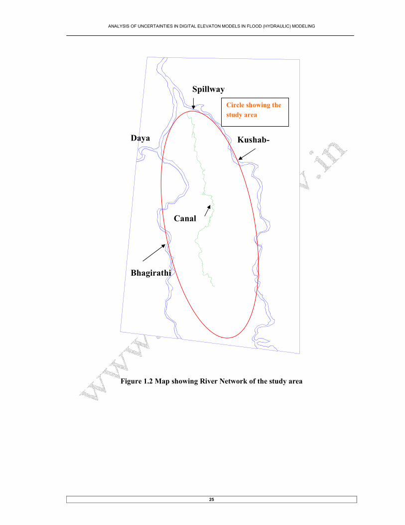
Figure 1.2 shows the main river network in part of Puri district, the two rivers Kushabhadra and
Bhagirathi splits from the main Mahanadi River. Daya River is a branch of Bhagirathi river. Kushab-
hadra River has been protected by the embankment on both the sides. During field visit in September
2004 it was observed that flooding is only in the downstream of the Kushabhadra river but on the up-
stream side of the river one spillway was built during the British period whose crest level is about two
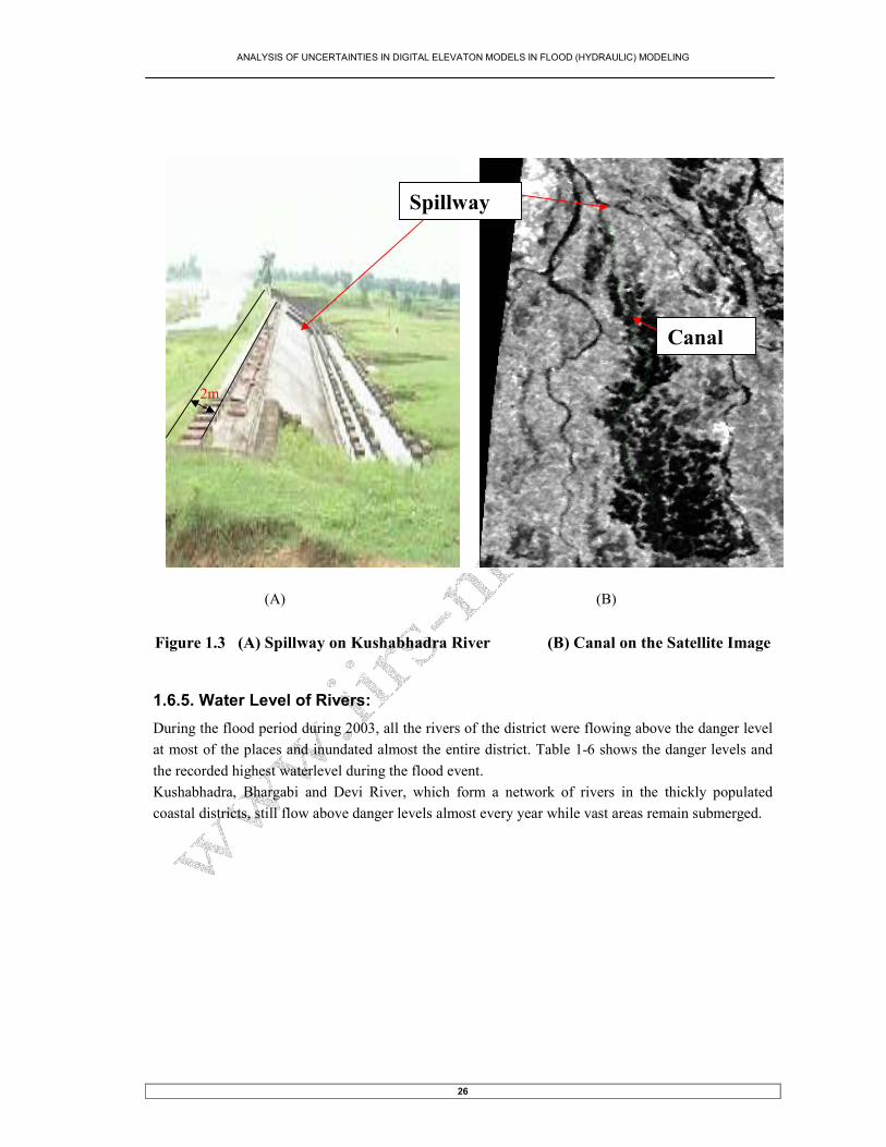
meter lower than the top of the embankment, as shown in Figure 1.2 and it was found that when the
water level reaches to the spillway water overflow from it. On behind the spillway there is an canal
which has been built to carry the excess water from the river. It can also be seen from the satellite im-
age of Radarsat (Figure 1.3 B) that flooding taken place around the canal.
ANALYSIS OF UNCERTAINTIES IN DIGITAL ELEVATON MODELS IN FLOOD (HYDRAULIC) MODELING
25
Bhagirathi
Daya
Spillway
Kushab-
Canal
Circle showing the
study area
Figure 1.2 Map showing River Network of the study area
ANALYSIS OF UNCERTAINTIES IN DIGITAL ELEVATON MODELS IN FLOOD (HYDRAULIC) MODELING
26
(A) (B)
Figure 1.3 (A) Spillway on Kushabhadra River (B) Canal on the Satellite Image
1.6.5. Water Level of Rivers:
During the flood period during 2003, all the rivers of the district were flowing above the danger level
at most of the places and inundated almost the entire district. Table 1-6 shows the danger levels and
the recorded highest waterlevel during the flood event.
Kushabhadra, Bhargabi and Devi River, which form a network of rivers in the thickly populated
coastal districts, still flow above danger levels almost every year while vast areas remain submerged.
Spillway
Canal
2m

ANALYSIS OF UNCERTAINTIES IN DIGITAL ELEVATON MODELS IN FLOOD (HYDRAULIC) MODELING
27
Table 1-6 Water level at different Gauge Station
Sr. No Name of
the
Irrigation
Division
River Gauge
Station
Danger
level in (m)
Highest water
level (m) re-
corded re-
cently
Date
1 Nimapara Kushabhadra Nimapara Bridge 3.25 3.35 30.8.03
2 Kushabhadra Jogisahi 17.44 18.28 30.8.03
3 Kushabhadra Sisumatha 15.08 16.14 1.9.03
4 Kushabhadra Gop 2.34 2.58 30.8.03
5 Bhargavi Achutapur 4.01 4.6 30.8.03
6 Bhargavi Balanga 3.16 3.53 30.8.03
7 Devi Baurikana 4.93 6.00 30.8.03
8 Puri Bhargavi Gabakund 6.77 6.76 30.8.03
9 Bhargavi Chandanpur Bridge 6.11 6.51 31.8.03
10 Bhargavi Haripur 11.67 12.20 1.9.03
11 Daya Madhipur 11.30 12.20 1.9.03
12 Daya Kanti 9.62 11.12 1.9.03
13 Daya Kanas 4.75 5.10 5.9.03
Source: Ministry of water recourses, water management wing Orissa
ANALYSIS OF UNCERTAINTIES IN DIGITAL ELEVATON MODELS IN FLOOD (HYDRAULIC) MODELING
28
2. Method and Material
2.1 Flood frequency analysis
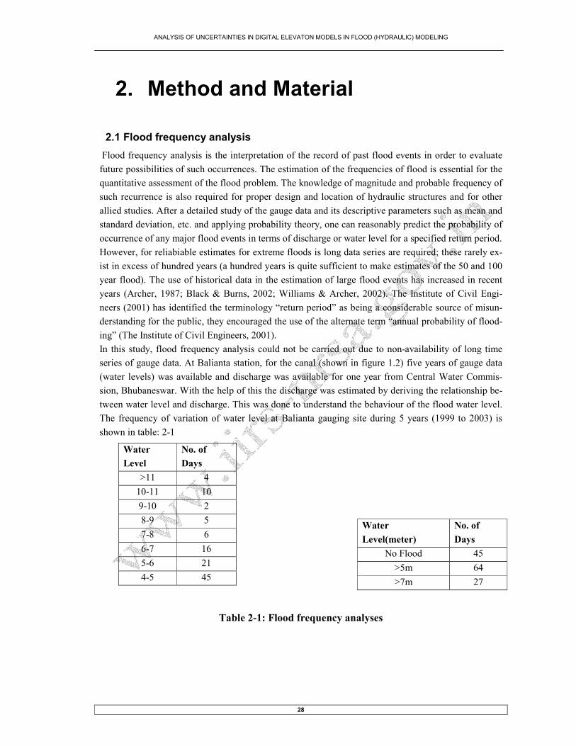
Flood frequency analysis is the interpretation of the record of past flood events in order to evaluate
future possibilities of such occurrences. The estimation of the frequencies of flood is essential for the
quantitative assessment of the flood problem. The knowledge of magnitude and probable frequency of
such recurrence is also required for proper design and location of hydraulic structures and for other
allied studies. After a detailed study of the gauge data and its descriptive parameters such as mean and
standard deviation, etc. and applying probability theory, one can reasonably predict the probability of
occurrence of any major flood events in terms of discharge or water level for a specified return period.
However, for reliabiable estimates for extreme floods is long data series are required; these rarely ex-
ist in excess of hundred years (a hundred years is quite sufficient to make estimates of the 50 and 100
year flood). The use of historical data in the estimation of large flood events has increased in recent
years (Archer, 1987; Black & Burns, 2002; Williams & Archer, 2002). The Institute of Civil Engi-
neers (2001) has identified the terminology “return period” as being a considerable source of misun-
derstanding for the public, they encouraged the use of the alternate term “annual probability of flood-
ing” (The Institute of Civil Engineers, 2001).
In this study, flood frequency analysis could not be carried out due to non-availability of long time
series of gauge data. At Balianta station, for the canal (shown in figure 1.2) five years of gauge data
(water levels) was available and discharge was available for one year from Central Water Commis-
sion, Bhubaneswar. With the help of this the discharge was estimated by deriving the relationship be-
tween water level and discharge. This was done to understand the behaviour of the flood water level.
The frequency of variation of water level at Balianta gauging site during 5 years (1999 to 2003) is
shown in table: 2-1
Table 2-1: Flood frequency analyses
Water
Level
No. of
Days
>11 4
10-11 10
9-10 2
8-9 5
7-8 6
6-7 16
5-6 21
4-5 45
Water
Level(meter)
No. of
Days
No Flood 45
>5m 64
>7m 27

ANALYSIS OF UNCERTAINTIES IN DIGITAL ELEVATON MODELS IN FLOOD (HYDRAULIC) MODELING
29
Figure 2.1: Stages (water level) Discharge Relationship (Power)
Using one year water level and discharge data, the stage-discharge relationships were established by
power and exponential relationships, which is shown in figure- 2.1 and 2.2 respectively. Since the
power relationship is having higher correlation coefficient, so power relationship is used for calculat-
ing discharge in further study. The equation used to calculate discharge was-
Y (discharge)= 1E-07e 0.7427x
(where x= water level and it values lies in between 26 to 34)
So in this way discharge was calculated for the upstream boundary condition and at the downstream
condition water level was taken as zero as it was very near to sea.
Chart Titley = 1E-07e
0.7427x
R2 = 0.8632
0
1000
2000
3000
4000
5000
6000
26 28 30 32 34
water level
discharge DISCHARGE
Expon.(DISCHARGE)
Figure 2.2: Stage (water level) Discharge Relationship (Exponential)
M3/sec
(m)
ANALYSIS OF UNCERTAINTIES IN DIGITAL ELEVATON MODELS IN FLOOD (HYDRAULIC) MODELING
30
Discharge
(m3/s)
Time (days)
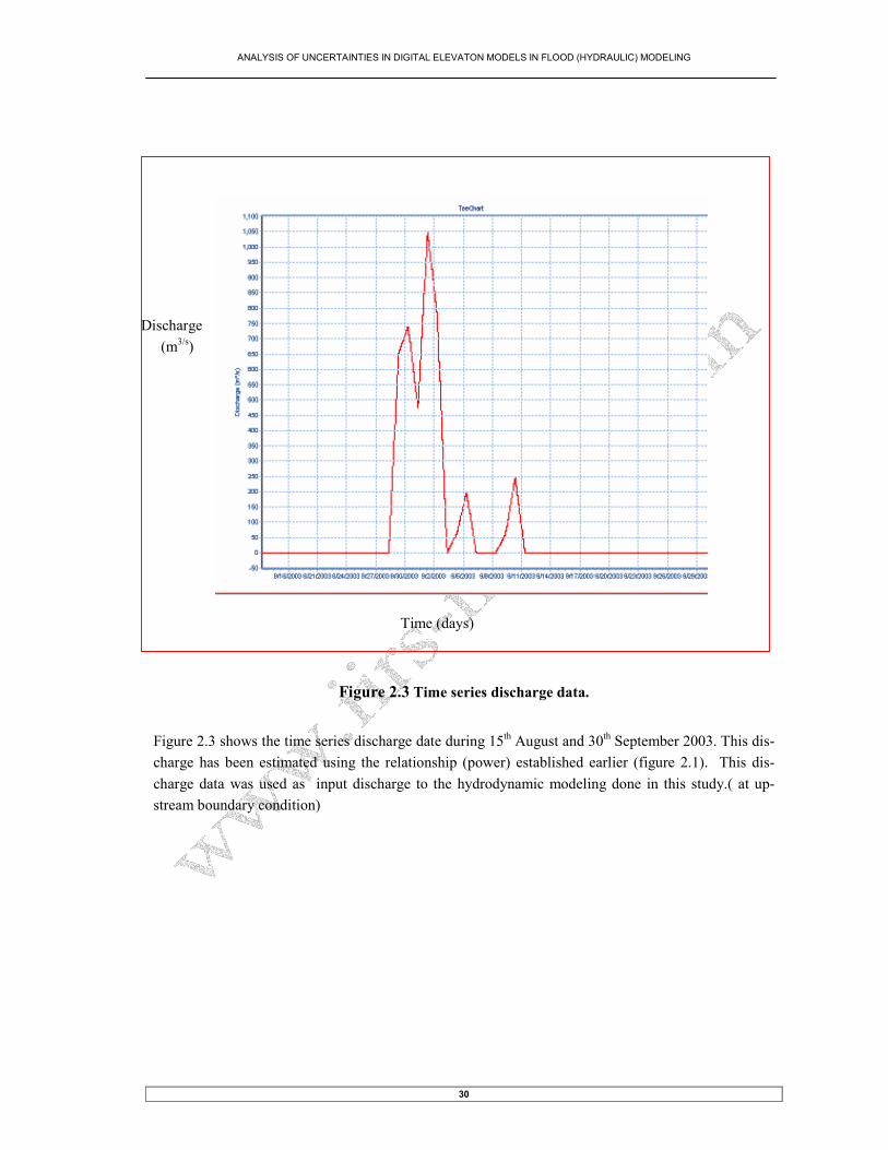
Figure 2.3 Time series discharge data.
Figure 2.3 shows the time series discharge date during 15th August and 30
th September 2003. This dis-
charge has been estimated using the relationship (power) established earlier (figure 2.1). This dis-
charge data was used as input discharge to the hydrodynamic modeling done in this study.( at up-
stream boundary condition)
Time (days)
ANALYSIS OF UNCERTAINTIES IN DIGITAL ELEVATON MODELS IN FLOOD (HYDRAULIC) MODELING
31
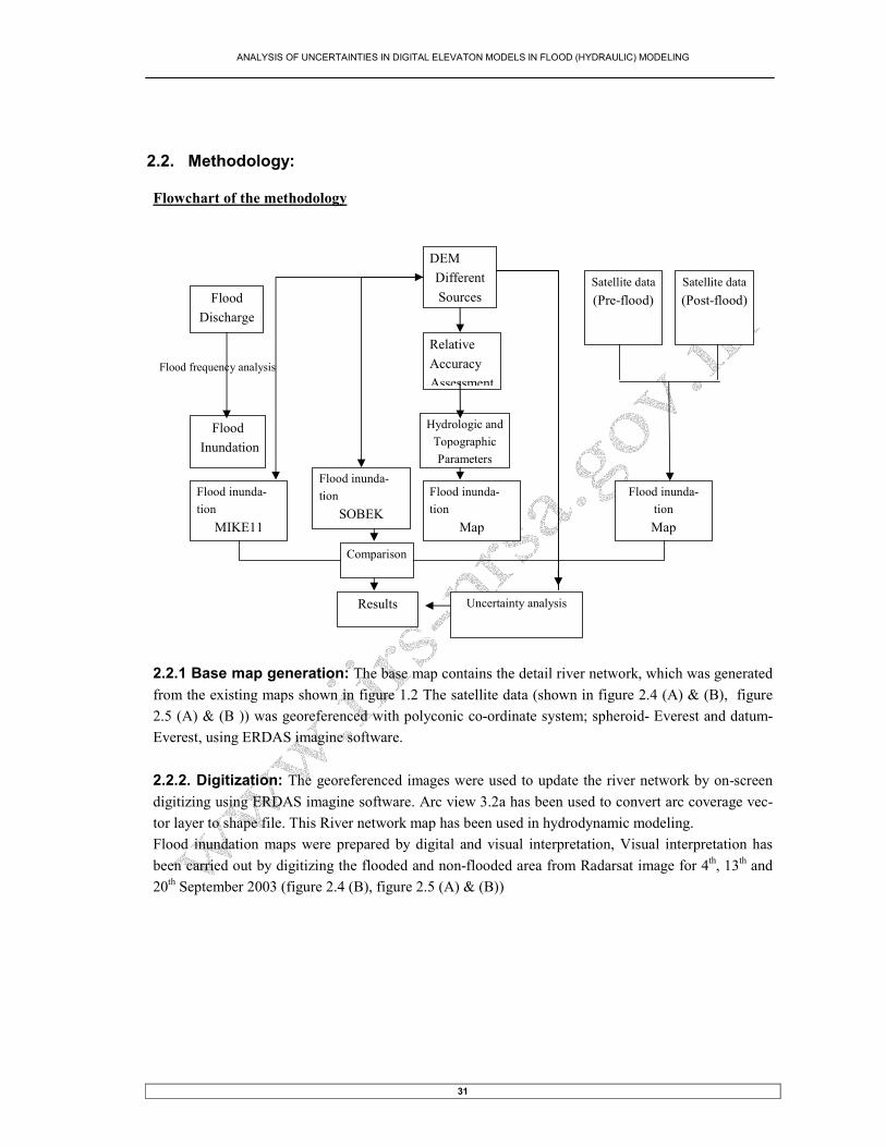
2.2. Methodology:
Flowchart of the methodology
2.2.1 Base map generation: The base map contains the detail river network, which was generated
from the existing maps shown in figure 1.2 The satellite data (shown in figure 2.4 (A) & (B), figure
2.5 (A) & (B )) was georeferenced with polyconic co-ordinate system; spheroid- Everest and datum-
Everest, using ERDAS imagine software.
2.2.2. Digitization: The georeferenced images were used to update the river network by on-screen
digitizing using ERDAS imagine software. Arc view 3.2a has been used to convert arc coverage vec-
tor layer to shape file. This River network map has been used in hydrodynamic modeling.
Flood inundation maps were prepared by digital and visual interpretation, Visual interpretation has
been carried out by digitizing the flooded and non-flooded area from Radarsat image for 4th, 13
th and
20th September 2003 (figure 2.4 (B), figure 2.5 (A) & (B))
Flood
Discharge
Flood
Inundation
Flood inunda-
tion
MIKE11
Flood inunda-
tion
SOBEK
Hydrologic and
Topographic
Parameters
Relative
Accuracy
Assessment
DEM
Different
Sources
Flood inunda-
tion
Map
Satellite data
(Pre-flood)
Satellite data
(Post-flood)
Flood inunda-
tion
Map
Uncertainty analysis
Comparison
Flood frequency analysis
Results
ANALYSIS OF UNCERTAINTIES IN DIGITAL ELEVATON MODELS IN FLOOD (HYDRAULIC) MODELING
32
2.3 Data Used:
2.3.1 Material used
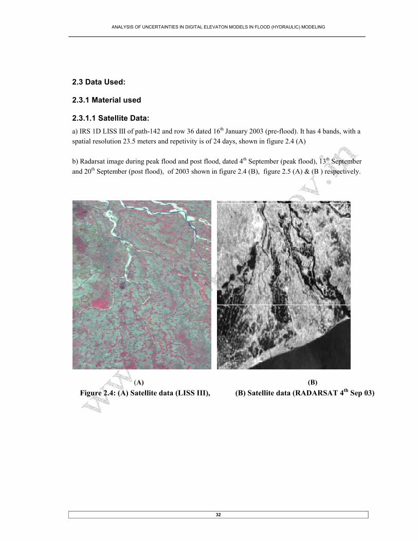
2.3.1.1 Satellite Data:
a) IRS 1D LISS III of path-142 and row 36 dated 16th January 2003 (pre-flood). It has 4 bands, with a
spatial resolution 23.5 meters and repetivity is of 24 days, shown in figure 2.4 (A)
b) Radarsat image during peak flood and post flood, dated 4th September (peak flood), 13th September
and 20th September (post flood), of 2003 shown in figure 2.4 (B), figure 2.5 (A) & (B ) respectively.
(A) (B)
Figure 2.4: (A) Satellite data (LISS III), (B) Satellite data (RADARSAT 4th Sep 03)

ANALYSIS OF UNCERTAINTIES IN DIGITAL ELEVATON MODELS IN FLOOD (HYDRAULIC) MODELING
33
(A) (B)
Figure 2.5: (A) Satellite data (RADARSAT 13th Sep), (B) Satellite data (RADARSAT 20
th September)
Ancillary Data:
Hydrological Data: Discharge of Balianta gauging site, water level of Balianta and at the spillway
and excess flood canal.
Topographic map:
Existing map was used for the generation of river network as shown in figure 2.6
Figure 2.6 River network

ANALYSIS OF UNCERTAINTIES IN DIGITAL ELEVATON MODELS IN FLOOD (HYDRAULIC) MODELING
34
2.3.1.2 DEM as a key parameter for hydrological modelling:
For hydrodynamic modeling a digital elevation model is also required, as explained in Para 1.2, but as
the study area is in restricted zone, DEM from the public domain which is available in internet is used
in this study. More detailed data not public?
Digital Elevation Model (DEM) is basic information for any three-dimensional (3-D) geo-spatial ac-
tivity. Many methodologies are currently being used to generate DEMs for different applications at
various scales, details and accuracy.
There are various methods that are commonly employed to generate DEMs for a variety of geo-spatial
applications these methods differ in technology, accuracy, comparative performance, economic viabil-
ity and cost effectiveness. The following is a brief description of these methods, which are going to be
used in hydraulic modeling.
a) Digital Extraction from Existing Topographic Maps
Digitization of contour lines from existing topographic maps is a traditional and relatively inexpensive
method to generate DEMs. Map digitization is still being used widely as means for creating DEMs for
certain applications. However, the study area as it is a restricted area so toposheet was not available,
so DEM could not be generated by contour.
b) DEM from ASTER
The ASTER sensor is designed to provide image data in 14 band from visible, near-infrared, short
wavelength infrared and thermal infrared spectral bands. Stereo image data are recorded only in Band
3, which is the near-infrared wavelength region from 0.78 to 0.86 ∝m, using both nadir and aft-
looking telescopes. From the nominal Terra altitude of 705 km, the ‘‘push broom’’ linear array sensor
covers a 60- km-wide ground track at a 15-m spatial resolution. A major advantage of the along-track
mode of data acquisition (as compared to cross-track) is that the images forming the stereopairs are
acquired a few seconds (rather than days) apart under uniform environmental and lighting conditions,
resulting in stereo pairs of consistent quality that are well suited for DEM generation by automated
stereo correlation techniques (Colvocoresses, 1982; Fujisada, 1994). The ASTER Digital Elevation
Model is a product that is generated from a pair of ASTER Level 1A images. This Level 1A input in-
cludes bands 3N (nadir) and 3B (aft-viewing) from the Visible & Near Infra-Red telescope's along-
track stereo data that is acquired in the spectral range of 0.78 to 0.86 microns, having a vertical accu-
racy of 7m and horizontal resolution of 30m. DEM from aster image is shown in Figure 2.7. Was also
available in public domain and it was downloaded from the internet. The minimum and maximum ele-
vation in the study area was in a range of 0 to 93 meters. Shown in figure 2.7(A)
Source: edcimswww.cr.usgs.gov, access on 25 September 2004.
c) DEM from SRTM (Shuttle Radar Topography Mission)
Synthetic Aperture Radar (SAR) is active Remote Sensing Systems. They emit microwave pulses,
which interact with the Earth's surface, and measure the backscattered signal. Obtained data has been
converted into height data called a Digital Elevation Model (DEM) and provided as public domain
data. Having a vertical accuracy of 16 m and Horizontal resolution of 90 m. The elevation information
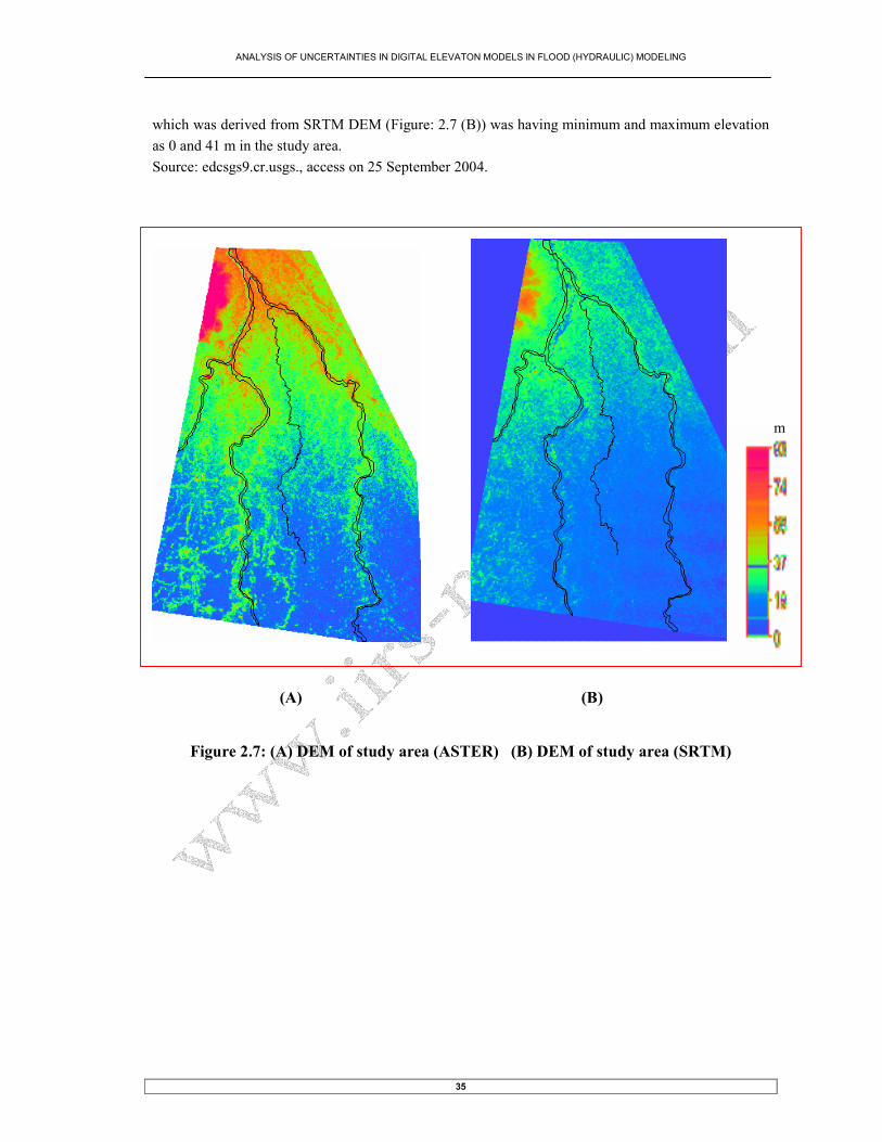
ANALYSIS OF UNCERTAINTIES IN DIGITAL ELEVATON MODELS IN FLOOD (HYDRAULIC) MODELING
35
which was derived from SRTM DEM (Figure: 2.7 (B)) was having minimum and maximum elevation
as 0 and 41 m in the study area.
Source: edcsgs9.cr.usgs., access on 25 September 2004.
A B
(A) (B)
Figure 2.7: (A) DEM of study area (ASTER) (B) DEM of study area (SRTM)
m

ANALYSIS OF UNCERTAINTIES IN DIGITAL ELEVATON MODELS IN FLOOD (HYDRAULIC) MODELING
36
DIGITAL INTERPETATION
Figure 2.8 Flood on 4th Sept Figure 2.9 Flood on 13th Sep Figure 2.10 Flood on 20th Sep
The flooded and non flooded area mapped using slicing technique in ILWIS (Integrated Land and Wa-
ter Information System) of three different dates 4th September 2003, 13
th September 2003 and 20
th
September 2003 were shown in figure 2.8, figure 2.9 and figure 2.10 respectively. To prepare the map
threshold digital number for water body was defined and then flood inundation maps were generated
by defining an IFF command. It was found that on 4th September about 212 km
2 of the study area was
inundated, that reduced to 147.57 km2 on 13th of September and further it reduced to 135.14 km2 on
20th of September.
To see the change in the spatial extent of inundation in the study area all the inundation map of 4th,
13th and 20
th September crossed and the temporal extent map was prepared shown in Figure 2.11.
N
Non-flooded
Flooded
Non-flooded
Flooded
Non flooded
Flooded

ANALYSIS OF UNCERTAINTIES IN DIGITAL ELEVATON MODELS IN FLOOD (HYDRAULIC) MODELING
37
Table 2-2: Area of flood inundation
Figure 2.11 Temporal flood extent map for 4th, 13th and 20th September
From the field knowledge and water level data, it was found that the water level was maximum on 1st
of September, 2003 which was about 30 m, peak flood on that day. The RADARSAT data that was
available, nearest to the peak flood event (of 4th September 2003) was used for the generation of flood
map.
VISUAL INTERPETATION
The visual interpretation of Radarsat images showed the total flooded area was 228.12 km2 , 151.87
km2 and 135 km2 on 4th , 13th and 20th September respectively.
Date Area of inunda-
tion(km2)
04.09.03 212.00
13.09.03 147.57
20.09.03 135.14
4th
13th
20th
Flooded area Non- flooded area
N
(a) (b) (c)

ANALYSIS OF UNCERTAINTIES IN DIGITAL ELEVATON MODELS IN FLOOD (HYDRAULIC) MODELING
38
Figure 2.12 Flood Inundation maps: a) 4th sept, 03 b) 13th sept, 03 c) 20th sept, 03
The flood inundation map generated using visual interpretation as shown in figure 2.12 was quite
similar to the flood inundation map generated through digital interpretation. Comparison of areal ex-
tent of flood inundation maps by visual interpretation and digital analysis is given in table 2-3
Table 2-3: Comparison between visual and digital interpretation
Date Visual Interpretation
Area (km2)
Digital Interpretation
Area (km2)
04.09.03 228.12 212.00
13.09.03 151.87 147.57
20.09.03 135.00 135.14
ANALYSIS OF UNCERTAINTIES IN DIGITAL ELEVATON MODELS IN FLOOD (HYDRAULIC) MODELING
39
3. Hydrodynamic Models
Hydrodynamic modelling is integration of various aspects of physics engineering and computer sci-
ence. It is based on conservation of mass and momentum, field & laboratory observation used to simu-
late the movements of fluids. Hydrodynamic models may be 1D, 2D, or 3D.
One-Dimensional Models
It is the simplest option which is best suited for representing flows within interconnected net-
works of channels. The channels are described by stream cross sections, and the model produces, for
each time step, water surface elevations at each cross section and average velocities between each
cross section. The disadvantage of one dimensional model is that it does not provide details of vertical
and horizontal velocity distributions, or circulation within large water bodies such as lakes, it does
yield accurate flows and is an adequate representation for many kinds of problems. One-dimensional
models have some capability to address problems beyond simple channel flow.
Advantages of one-dimensional models as follows:
� In one dimensional models computations are fast.
� Relatively little field data is required to set up the models.
� Traditionally one-dimensional models have more powerful capabilities to describe control structures than do higher-dimensional models when used for flood prediction.
Two-Dimensional
In two-dimensional models lateral circulation in large water-bodies are considered and the flow char-
acteristics are assumed to be uniform down through the water column at each computational point, so
that stratification is not described.
The disadvantages of the model are:
� It is time consuming
� It requires more field data than the one dimensional model
� It do not describe the control structures compared to one dimensional models
Two-dimensional models require significantly more computer resources (memory and runtime) than
do one-dimensional models. Therefore, it is necessary to perform a trade-off between the density of
the computational network used to define the model area, and the15resultant run-times, requirements
for computer memory, and disk storage space. (Moffatt and Nichol 2003)
3.1 Data Requirement (Hydrodynamic models)
1) Basic data:
This is mainly data that describes the physical layout of the river or the catchments being modelled.
This includes for instance cross-section, weir crest level and dimensions, catchments area etc. Which
in this case, the Mahanadi river is split into Bagirathi and Kushabhadra rivers. There is a canal con-

ANALYSIS OF UNCERTAINTIES IN DIGITAL ELEVATON MODELS IN FLOOD (HYDRAULIC) MODELING
40
structed from Kushabhadra River to relieve the overflow of water through a spillway (shown in Fig.
1.2).
2) Parameters:
This covers parameters that are used in the equations being solved by hydraulic model. Examples of
such parameters are Manning’s coefficients and weir contraction/expansion loss coefficients. How-
ever most parameters have to be estimated through calibration / verification, literature review or from
experience.
3) Boundary data:
Models requires boundary conditions, and typically these are time series of measurements such as dis-
charge, water level etc. at the boundaries of the modelled (schematised) area (these are the connec-
tions between your model-reality and the rest of the universe!).
4) Calibration and verification data:
These data are actually not required to run the model, i.e. to produce simulation results. Having the
data group 1-3 available is sufficient assuming that the parameters have been estimated properly.
However, this is most often not possible without calibration and verification, and to do so additional
data are required. This is for instant time series of measurements of discharge, water level and river
bed level or RS-imagery to check flood extent. This is relevant for this study.
3.2. MIKE 11 model
MIKE 11, developed by Danish Hydraulic Institute (DHI) Water & Environment, is a modeling pack-
age for the simulation of surface runoff, flow, sediment transport and water quality in rivers, flood-
plains, channels and channels. The hydrodynamic module (MIKE11 HD) is commonly applied as a
flood management tool simulating the unsteady flow in branched and looped river networks and quasi
two-dimensional flow on floodplains. Once a model is established and calibrated, the impact of
change of artificial or natural origin of flood behaviour can be quantified and displayed as change in
flood level and discharges.
MIKE 11 is based on an effective numerical solution of the complete non-linear St-Venant equation
for 1-D flows. A network editor assists the schematization of rivers and floodplain as a system of in-
ter-connected branches. Flood level and discharges as a function of time are calculated at specific
points along the branches to describe the passage of flood flows through the model domain. MIKE11
HD operates based on information about river and floodplain topography, which may include man-
made flood control measures and hydro meteorological boundary conditions.
DHI's MIKE 11 software package is a versatile and modular engineering tool for modeling conditions
in rivers, lakes/reservoirs, irrigation canals and other inland water system (URL3). It is designed for:
• Flood risk analysis and mapping
• Design of flood alleviation systems
• Real-time flood forecasting

ANALYSIS OF UNCERTAINTIES IN DIGITAL ELEVATON MODELS IN FLOOD (HYDRAULIC) MODELING
41
• Hydraulic analysis/design of structures including bridges
• Drainage and irrigation studies
• Optimization of river and reservoir operations
• Dam break analysis
• water quality issues
• Integrated groundwater and surface water analysis
Mike11 consists of following Editor –
1) Simulation Editor
2) River Network Editor
3) Cross Section Editor
4) Boundary Editor
5) Rainfall-Runoff Editor
6) Hydrodynamic Editor
7) Advection-Dispersion Editor
8) WQ ECO lab Editor
9) WQ (BOD/DO) Editor
10) Sediment Transport Editor
11) Flood Forecasting Editor
12) Batch Simulation Editor
In this thesis only hydrodynamic modeling, has been done hence used only –
Simulation Editor
River Network Editor
Cross Section Editor
Boundary Editor and
Hydrodynamic Editor
3.2.1. Simulation Editor:
The Simulation Editor serves various purposes:
Selection of the models for analysis and also simulation mode, selection of input files for simulation
i.e. Network, cross-section, Boundary data and hydrodynamic (HD) parameters.
• Selecting the time period.
• Defining the result file.
Figure 3.1 shows the choice of the models available in MIKE 11. In this case only hydrodynamic
model and unsteady simulation model is used.
Figure 3.2 shows the window where the input files are defined. Various input parameters required for
hydrodynamic model such as network, cross-section, boundary data and rainfall-runoff parameters can
be edited also using this window.

ANALYSIS OF UNCERTAINTIES IN DIGITAL ELEVATON MODELS IN FLOOD (HYDRAULIC) MODELING
42
A B
Figure 3.1: Main Window of hydrodynamic model (A) and main window showing input file (B)
In Input parameters for hydrodynamic modeling are-
These are the names of your input files?
1) Network files. (length. Nwk11)
2) Cross-section files. ( cross-section length1. Xns11)
3) Boundary files. (boundary .bnd11) ( Upstream U1 & Downstream U2)
4) HD parameter files. HD11
Network file can be input to the model by digitizing in the editor with the help of raster map in the
background or earlier digitized river network as shape file can be imported into MIKE 11.

ANALYSIS OF UNCERTAINTIES IN DIGITAL ELEVATON MODELS IN FLOOD (HYDRAULIC) MODELING
43
(a) (b)
Figure 3.2: Network files (* .nwk11 format) (a) & (b) River network
Figure 3.2 (a) shows the canal of the study area, which has been imported in MIKE 11 as a shape file.
The segment was drawn across the canal at some distance, approximately until the extent of flood on
both side of the canal to calculate the cross-section.
3.2.2 Generation of cross-section in MIKE 11 GIS
U1
U2
U1
U2
A B C

ANALYSIS OF UNCERTAINTIES IN DIGITAL ELEVATON MODELS IN FLOOD (HYDRAULIC) MODELING
44
Figure 3.3: (A) ASTER DEM image (B) Canal over the image (C) Elevation extracted on
the segment

ANALYSIS OF UNCERTAINTIES IN DIGITAL ELEVATON MODELS IN FLOOD (HYDRAULIC) MODELING
45
In the ASTER DEM shown in figure 3.3 (A) the canal has been added on it, (shown in figure 3.3 (B))
To obtain the cross-section elevation on both sides of the canal, segment have been drawn, perpen-
dicular across the canal, (shown in figure 3.3 (C) in MIKE 11 GIS Software, the segment was crossed
with the pixel value to obtained the elevation information. Thus MIKE 11 GIS itself generate water
level information, and discharge valve in between the water level point in form of Microsoft access
file. Thus water level point was taken at wherever segment point has crossed with canal. Thus the
cross-section details of the flood plain but not of river have been determined. Figure 3.4 showing the
segment drawn on the Q-H points and the elevation extracted on the segments from the ASTER DEM.
Figure 3.4: Segment over the Q-H point
Figure 3.5: Cross-section Editor window in the river
Figure 3.6: Location of the cross-section
The location of the river cross-sections generated in MIKE 11 is shown in the figure 3.6.
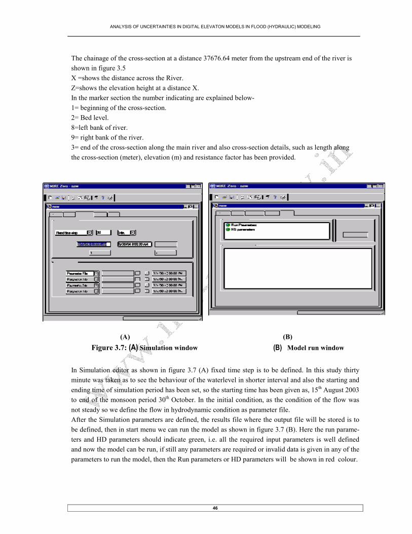
ANALYSIS OF UNCERTAINTIES IN DIGITAL ELEVATON MODELS IN FLOOD (HYDRAULIC) MODELING
46
The chainage of the cross-section at a distance 37676.64 meter from the upstream end of the river is
shown in figure 3.5
X =shows the distance across the River.
Z=shows the elevation height at a distance X.
In the marker section the number indicating are explained below-
1= beginning of the cross-section.
2= Bed level.
8=left bank of river.
9= right bank of the river.
3= end of the cross-section along the main river and also cross-section details, such as length along
the cross-section (meter), elevation (m) and resistance factor has been provided.
(A) (B)
Figure 3.7: (A) Simulation window (B) Model run window
In Simulation editor as shown in figure 3.7 (A) fixed time step is to be defined. In this study thirty
minute was taken as to see the behaviour of the waterlevel in shorter interval and also the starting and
ending time of simulation period has been set, so the starting time has been given as, 15th August 2003
to end of the monsoon period 30th October. In the initial condition, as the condition of the flow was
not steady so we define the flow in hydrodynamic condition as parameter file.
After the Simulation parameters are defined, the results file where the output file will be stored is to
be defined, then in start menu we can run the model as shown in figure 3.7 (B). Here the run parame-
ters and HD parameters should indicate green, i.e. all the required input parameters is well defined
and now the model can be run, if still any parameters are required or invalid data is given in any of the
parameters to run the model, then the Run parameters or HD parameters will be shown in red colour.

ANALYSIS OF UNCERTAINTIES IN DIGITAL ELEVATON MODELS IN FLOOD (HYDRAULIC) MODELING
47
(A) (B)
Figure 3.8: (A) Boundary Editor (B) Hydrologic parameters
The Figure 3.8 (A) is the Boundary Editor where the boundary description and type at the upstream
and downstream condition are given as for upstream condition the water level was at the height of 26
m and for the downstream condition, water level was at a height of 0 m from mean sea level. (Shown
in figure 1.2 U1 & U2) In the chainage section river length is define. In this boundary editor there is
an edit section where the time series data of discharge starting from 15th August to 30
th October is
given. In figure 3.8 (B) showing hydrological parameters, such as initial water condition, reach length,
flood plain resistance etc have to be defined. They where defined based on the field conditions.
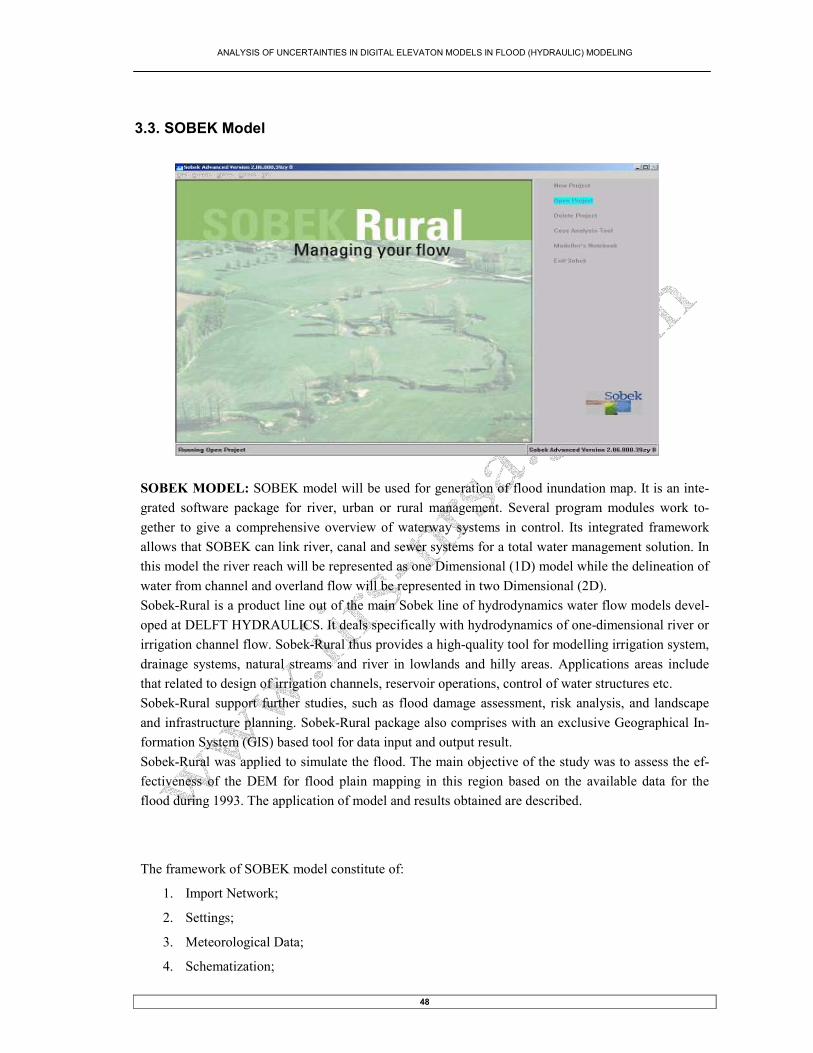
ANALYSIS OF UNCERTAINTIES IN DIGITAL ELEVATON MODELS IN FLOOD (HYDRAULIC) MODELING
48
3.3. SOBEK Model
SOBEK MODEL: SOBEK model will be used for generation of flood inundation map. It is an inte-
grated software package for river, urban or rural management. Several program modules work to-
gether to give a comprehensive overview of waterway systems in control. Its integrated framework
allows that SOBEK can link river, canal and sewer systems for a total water management solution. In
this model the river reach will be represented as one Dimensional (1D) model while the delineation of
water from channel and overland flow will be represented in two Dimensional (2D).
Sobek-Rural is a product line out of the main Sobek line of hydrodynamics water flow models devel-
oped at DELFT HYDRAULICS. It deals specifically with hydrodynamics of one-dimensional river or
irrigation channel flow. Sobek-Rural thus provides a high-quality tool for modelling irrigation system,
drainage systems, natural streams and river in lowlands and hilly areas. Applications areas include
that related to design of irrigation channels, reservoir operations, control of water structures etc.
Sobek-Rural support further studies, such as flood damage assessment, risk analysis, and landscape
and infrastructure planning. Sobek-Rural package also comprises with an exclusive Geographical In-
formation System (GIS) based tool for data input and output result.
Sobek-Rural was applied to simulate the flood. The main objective of the study was to assess the ef-
fectiveness of the DEM for flood plain mapping in this region based on the available data for the
flood during 1993. The application of model and results obtained are described.
The framework of SOBEK model constitute of:
1. Import Network;
2. Settings;
3. Meteorological Data;
4. Schematization;

ANALYSIS OF UNCERTAINTIES IN DIGITAL ELEVATON MODELS IN FLOOD (HYDRAULIC) MODELING
49
5. Simulation;
6. Results in Maps;
7. Results in Charts;
8. Result in tables.
In the Case manager, figure 3.9. given below, each block represents a specific task. A task can be a
model, or a set of linked models, or the selection of a scenario or strategy, or a (graphical) presenta-
tion tool.
Figure 3.9: Case manager
The colour of each block represents the status of running the model. They are
1. Yellow: the task can be executed;
2. Green: the task has been executed at least once and can be executed again;
3. Red: the task cannot be executed until the preceding task has been executed
3.3.1. Import Network
Import network as shown in figure 3.10 is used to define the network file from where it will be im-
ported. We can also digitize the river network for this it is necessary to define as start from scratch.
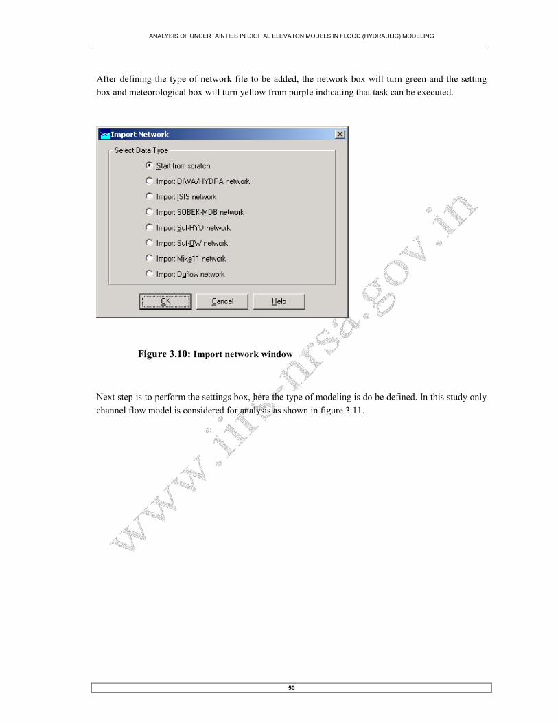
ANALYSIS OF UNCERTAINTIES IN DIGITAL ELEVATON MODELS IN FLOOD (HYDRAULIC) MODELING
50
After defining the type of network file to be added, the network box will turn green and the setting
box and meteorological box will turn yellow from purple indicating that task can be executed.
Figure 3.10: Import network window
Next step is to perform the settings box, here the type of modeling is do be defined. In this study only
channel flow model is considered for analysis as shown in figure 3.11.
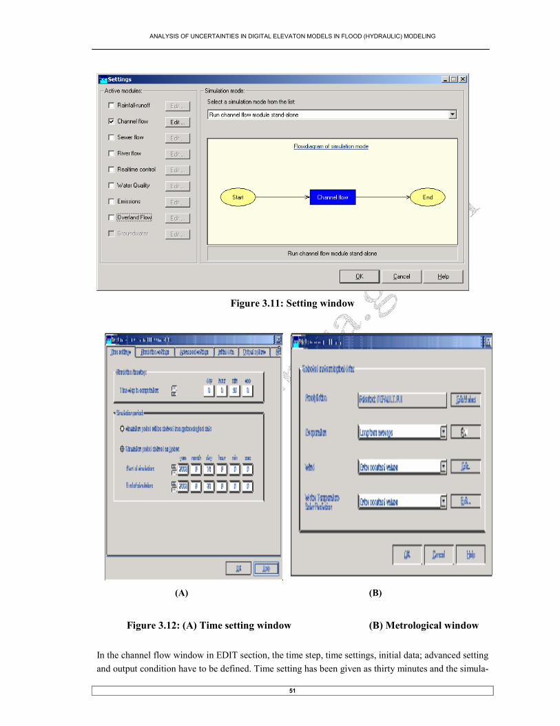
ANALYSIS OF UNCERTAINTIES IN DIGITAL ELEVATON MODELS IN FLOOD (HYDRAULIC) MODELING
51
Figure 3.11: Setting window
(A) (B)
Figure 3.12: (A) Time setting window (B) Metrological window
In the channel flow window in EDIT section, the time step, time settings, initial data; advanced setting
and output condition have to be defined. Time setting has been given as thirty minutes and the simula-

ANALYSIS OF UNCERTAINTIES IN DIGITAL ELEVATON MODELS IN FLOOD (HYDRAULIC) MODELING
52
tion period is defined from 15th August to 30
th September 2003 shown above in figure 3.12 (A), simi-
lar to MIKE 11 simulation.
In the meteorological data box, figure 3.12 (B). It has been left as default, as the rainfall-runoff analy-
sis are not considered, so these factors can be neglected When the option <Edit Model> of the ‘Sche-
matisation’ in figure 3.19. is selected, the network editor starts. The network editor is called NETTER
and is a component of the Delft Hydraulics Decision Support System (Delft-DSS) tools. NETTER
offers the possibility to set-up the Schematisation on top of a background GIS map. NETTER also
offers advanced analysis tools to show model results attached to the schematisation.
Within NETTER the following can be done:
1. Interactively and graphically prepare a schematisation;
2. Generate schematisation upon GIS map Layers;
3. Carry out schematisation operations: search for a certain node, show node numbers and
Names show link numbers, etc.
4. Carry out map operations: zooming in, zooming out, (de)activating map layers,
Colouring of map layers, adding title information on the map, etc.
5. View results of simulation models for schematisation created in NETTER;
Generally speaking, NETTER has two edit modes. The first mode is the mode to set-up the schemati-
sation, e.g. by adding new nodes. The second edit mode is the mode for editing the attribute data. In
this mode you give attributes to the schematisation objects.
So after completing these three-editor sections we can perform the stimulation editor. Here in the
Schematisation it can be edited and add or digitized river network and add the boundary and cross-
section of the river at the desire co-ordinate point in the netter developer. Here the digitization of the
river network has been carried out and specified the branch location and cross-section as shown below
in figure 3.14.
Figure 3.13: Schematisation Box
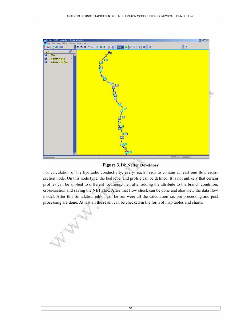
ANALYSIS OF UNCERTAINTIES IN DIGITAL ELEVATON MODELS IN FLOOD (HYDRAULIC) MODELING
53
Figure 3.14: Netter Developer
For calculation of the hydraulic conductivity, every reach needs to contain at least one flow cross-
section node. On this node type, the bed level and profile can be defined. It is not unlikely that certain
profiles can be applied to different locations, then after adding the attribute to the branch condition,
cross-section and saving the NETTER. After that flow check can be done and also view the data flow
model. After this Simulation editor can be run were all the calculation i.e. pre processing and post
processing are done. At last all the result can be checked in the form of map tables and charts.

ANALYSIS OF UNCERTAINTIES IN DIGITAL ELEVATON MODELS IN FLOOD (HYDRAULIC) MODELING
54
4.0 Analysis and Result
4.1 MIKE 11 Model using ASTER DEM
Comparison has been done with hydrodynamic model, which has been used to determine the flood
inundation as explained in chapter III and flood inundation from satellite images in Figure 2.8. The
digital elevation models (DEM) used in hydrodynamic models is ASTER and SRTM.
4.1.1 Longitudinal profile of study area using ASTER DEM
Using ASTER DEM, the longitudinal profile of the canal, which is investigated in this study, has been
generated. The below figure (4.1) shows the longitudinal profile details of the canal showing the de-
tails of the left and right flood plain, initial water level and the maximum water depth reached during
the peak discharge derived by MIKE 11 model. Using ASTER DEM, showing the elevation informa-
tion for the whole area of the flood plain, cross-section profile has generated in MIKE 11 view, which
is result-viewing software as a part of MIKE 11. The elevation information shows at starting point in
the river having an elevation on the right levee bank of 37 meter and on left levee bank showing 30
meter. At the downstream end of the river we got 15 meter height on right levee bank while on left
levee bank it showing 14 meter height. In the below profile (Figure: 4.1) derived in MIKE 11 using
aster DEM.
The graph has been plotted by MIKE 11 model between simulated discharge and height (Q-H curve)
at different reaches during the entire period of simulation of the river. This is shown in below figures
(4.2, 4.3, 4.4 & 4.5) at a distance for 713.41m, 1041m, 15613.25m, and 44641.65m respectively. At a
distance of 713.41 meter at a height of 26 meter, the discharge was 0 and at the maximum discharge
about 1050 cubic meter per second the waterlevel reaches a height of 32 meter, likewise at a distance
of 1041m, 15613.25m and at 44641.65m discharge crossing the different height is shown in the figure
number: 4.3, 4.4, & 4.5 respectively. The discharge and height relationship on 4th, 13
th, and 20
th on
which satellite data was acquired at different chainage distance is also shown in the figure respec-
tively

ANALYSIS OF UNCERTAINTIES IN DIGITAL ELEVATON MODELS IN FLOOD (HYDRAULIC) MODELING
55
Figure 4.1: Longitudinal profile derived using ASTER DEM.
Left
bank
Right
bank
Bed level
Distance (m) along the canal
Height
(m)
Above
mean
sea
level
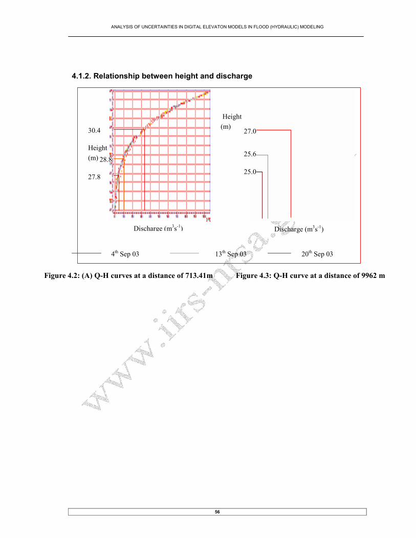
ANALYSIS OF UNCERTAINTIES IN DIGITAL ELEVATON MODELS IN FLOOD (HYDRAULIC) MODELING
56
4.1.2. Relationship between height and discharge
Figure 4.2: (A) Q-H curves at a distance of 713.41m Figure 4.3: Q-H curve at a distance of 9962 m
Discharge (m3s-1)
Height
(m)
Discharge (m3s-1)
Height
(m)
4th Sep 03 13th Sep 03 20th Sep 03
25.0
25.6
27.0 30.4
27.8
28.8

ANALYSIS OF UNCERTAINTIES IN DIGITAL ELEVATON MODELS IN FLOOD (HYDRAULIC) MODELING
57
Discharge (m3s-1) Discharge (m
3s-1)
Figure 4.4: Q-H curves at a distance 15613.25m Figure 4.5: Q-H curve at a distance 44641.65m
16.0 22.2
10.9
10.3
Height
(m)
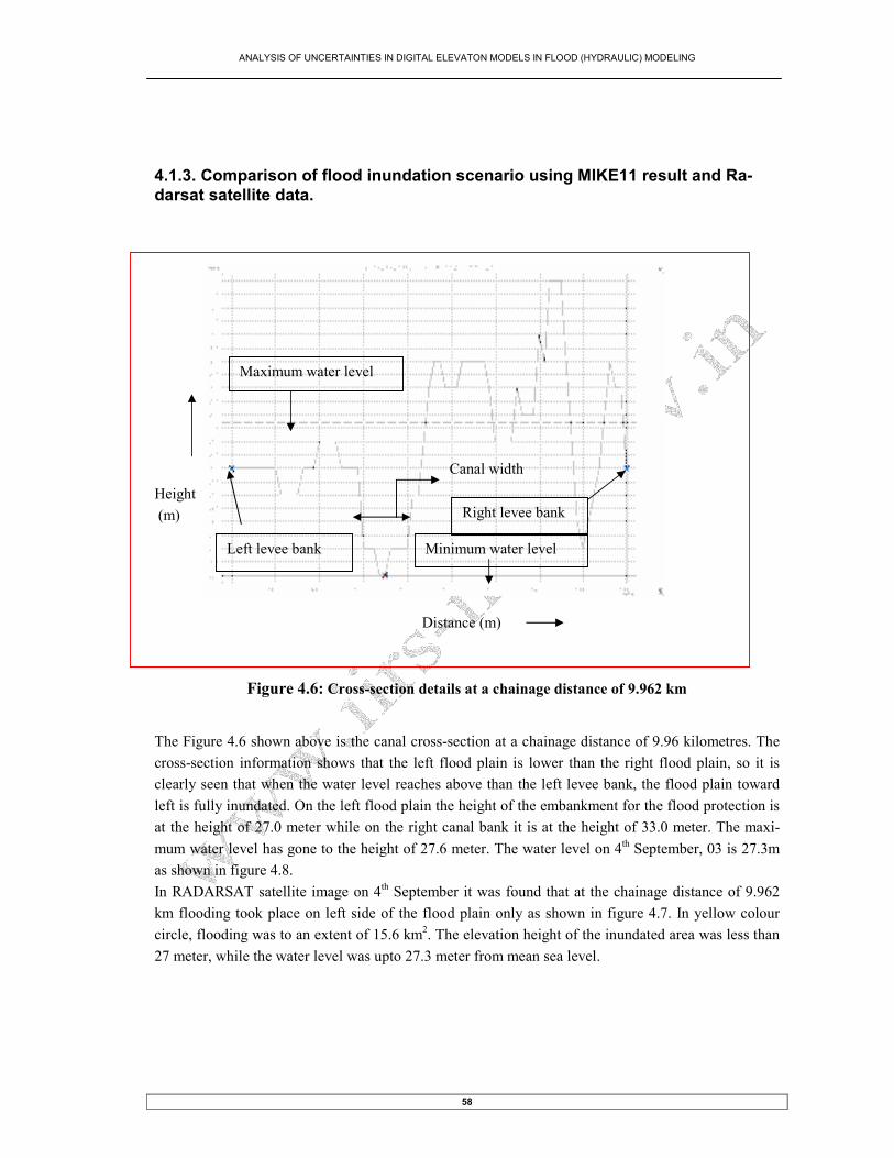
ANALYSIS OF UNCERTAINTIES IN DIGITAL ELEVATON MODELS IN FLOOD (HYDRAULIC) MODELING
58
4.1.3. Comparison of flood inundation scenario using MIKE11 result and Ra-
darsat satellite data.
Height
(m)
Distance (m)
Figure 4.6: Cross-section details at a chainage distance of 9.962 km
The Figure 4.6 shown above is the canal cross-section at a chainage distance of 9.96 kilometres. The
cross-section information shows that the left flood plain is lower than the right flood plain, so it is
clearly seen that when the water level reaches above than the left levee bank, the flood plain toward
left is fully inundated. On the left flood plain the height of the embankment for the flood protection is
at the height of 27.0 meter while on the right canal bank it is at the height of 33.0 meter. The maxi-
mum water level has gone to the height of 27.6 meter. The water level on 4th September, 03 is 27.3m
as shown in figure 4.8.
In RADARSAT satellite image on 4th September it was found that at the chainage distance of 9.962
km flooding took place on left side of the flood plain only as shown in figure 4.7. In yellow colour
circle, flooding was to an extent of 15.6 km2. The elevation height of the inundated area was less than
27 meter, while the water level was upto 27.3 meter from mean sea level.
Right levee bank
Left levee bank Minimum water level
Maximum water level
Canal width

ANALYSIS OF UNCERTAINTIES IN DIGITAL ELEVATON MODELS IN FLOOD (HYDRAULIC) MODELING
59
Figure 4.7: RADARSAT image on 4th September

ANALYSIS OF UNCERTAINTIES IN DIGITAL ELEVATON MODELS IN FLOOD (HYDRAULIC) MODELING
60
Height
(m)
Distance (m)
Figure 4.8: Water level on 4th September.
In the above figure (4.8) it can be seen that water level has crossed the left channel bank of the river at
a chainage distance of 9.96 kilometer on 4th September, 03. and in the below figure (4.9) the water
level is maximum on 1st September. It can be also seen that on 4
th September water level has rise to 27
meter while on 1st September, 03 (figure 4.9) it had reached up to 27.6 meter. While confirmation was
made during field that the flooding start on 29th of August and on 1
st of September flooding was maxi-
mum.
Height
(m)
Distance (m)
Figure 4.9: Water level on 1ST September, 2003
Water Level
Right levee bank
Water Level
Right Levee Bank
Canal Width
Canal Width

ANALYSIS OF UNCERTAINTIES IN DIGITAL ELEVATON MODELS IN FLOOD (HYDRAULIC) MODELING
61
Figure 4.10 and 4.11 shows the water level on 13th and 20
th September, 2003 respectively. Water level
on 13th as well as on 20th September is showing below the embankment of the river, so flooding has
not taken place at this chainage. Comparing was done with the flood inundation map generated by
Radarsat image, as shown in figure 2.11. It was found that flooding has not occurred in this area on
13th and 20th September, 03.
Height
(m)
Distance(m)
Figure 4.10: Water level on 13th September, 03
4.1.4. Water level and Flood depth
In the figure below (4.11), shows the water level in the longitudinal profile of the area on 4th Septem-
ber. Here in the graph Y-axis represents the elevation, and on the X-axis it showing the chainage dis-
tance of the canal. By viewing this profile it was make out that, from the upstream end to 0.6 kilome-
tre flooding is happening on the left levee bank and than from 0.0 kilometre to 5.6 kilometre flooding
is happening on left levee bank, than from the distance 5.6 to 7.9 kilometres it is on the right side of
the canal than from 20.1 to 30.8 kilometre flooding does not occur from the canal and than from the
distance 33.8 kilometre to the downstream flooding has been on both side of the canal. The maximum
water level reaches to 22 meter from mean sea level on the downstream side.
In this figure colour line which indicate different banks and parameters are explained below-
Cyan colour =Water level
Yellow line = Left levee bank
Brown line = Right levee bank
Blue line = Lowest point in cross-section (bed level)
Left Bank
Right Bank
Water level
Right Levee Bank
Canal Width

ANALYSIS OF UNCERTAINTIES IN DIGITAL ELEVATON MODELS IN FLOOD (HYDRAULIC) MODELING
62
Height
(m)
Distance (m)
Figure 4.11: Water level on 4th September
In figure (4.12) shows the discharge, flood depth and water level. Here on X-axis representing the
river chainage distance in meter and on Y-axis on left side it is representing the elevation in meter and
on right side discharge in meter cube per second.
Height
(m)
Distance (m)
Figure 4.12: Flood level in the river reach on 4th September
Water
Discharge
Flood Depth

ANALYSIS OF UNCERTAINTIES IN DIGITAL ELEVATON MODELS IN FLOOD (HYDRAULIC) MODELING
63
4.2 MIKE 11 Model using SRTM DEM
4.2.1. Longitudinal profile of study area using SRTM DEM
Using SRTM DEM, the Longitudinal profile of the canal from Kushabhadra river reach has been
generated The below figure (4.13) shows the longitudinal profile details of the canal showing the de-
tails of the left and right flood plain and the maximum water depth reached during the peak discharge.
Using SRTM DEM, showing the elevation information for the whole area of the flood plain, cross-
section profile has generated in MIKE 11 viewer. The elevation information shows at starting point in
the river having an elevation on the right levee bank of 20 meter and on left levee bank also showing
20 meter. At the downstream end of the river we got 09-meter height on right levee bank while on left
levee bank it showing 08-meter height. (shown in figure 4.13)
Discharge (m)
Height
(m)
Distance (m)
Figure 4.13: Longitudinal profile derived using SRTM DEM.
Left Bank
Right Bank
Bed Level

ANALYSIS OF UNCERTAINTIES IN DIGITAL ELEVATON MODELS IN FLOOD (HYDRAULIC) MODELING
64
4.2.2. Relationship between height and discharge
The graph has been plotted by using Mike 11 model between discharge and height (Q-H curve) at dif-
ferent reaches during the entire period of simulation of the river. This is shown in below figures (4.14,
4.15, 4.16 & 4.17) at a distance for 713.41m, 1041m, 15613.25m, and 44641.65m respectively. At a
distance of 713.41 meter the discharge was 0 at a height of 19.1 meter and at the maximum discharge
about 1050 cubic meter per second it crosses the height of 20 meter, likewise at a distance of 1041m,
15613.25m and at 44641.65m discharge crossing the different height is shown in the figure number:
4.15, 4.16, & 4.17 respectively.
Height
(m)
Figure 4.14: Q-H curves at a distance of 713.41m Figure 4.15: Q-H curve at a distance of 1041m
Discharge (m3s-1)
19.1
18.6
18.3
17.8
17.2
16.8

ANALYSIS OF UNCERTAINTIES IN DIGITAL ELEVATON MODELS IN FLOOD (HYDRAULIC) MODELING
65
Height
(m)
Figure 4.16: Q-H curve at a distance 15613.25m Figure 4.17: Q-H curve at a distance 44641.65m
4.2.3. Comparison of flood inundation scenario using MIKE11 results and RA-
DAR satellite data
Height
(m)
Distance (m)
Figure 4.18: Cross-section details at a chainage distance of 9.962 km
Discharge (m3s-1) Discharge (m
3s-1)
13.1
12.2
11.2
10.4
Water Level
Right Levee Bank
Canal Width
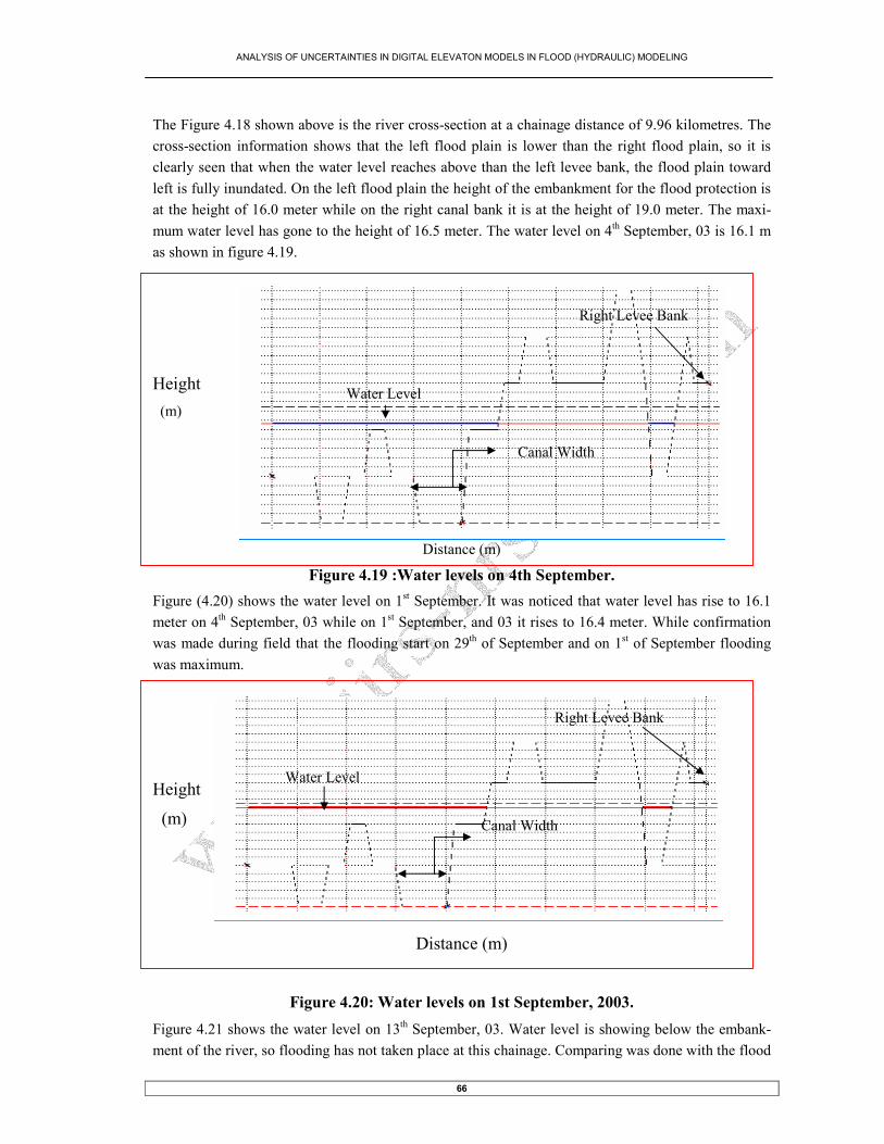
ANALYSIS OF UNCERTAINTIES IN DIGITAL ELEVATON MODELS IN FLOOD (HYDRAULIC) MODELING
66
The Figure 4.18 shown above is the river cross-section at a chainage distance of 9.96 kilometres. The
cross-section information shows that the left flood plain is lower than the right flood plain, so it is
clearly seen that when the water level reaches above than the left levee bank, the flood plain toward
left is fully inundated. On the left flood plain the height of the embankment for the flood protection is
at the height of 16.0 meter while on the right canal bank it is at the height of 19.0 meter. The maxi-
mum water level has gone to the height of 16.5 meter. The water level on 4th September, 03 is 16.1 m
as shown in figure 4.19.
Height
(m)
Distance (m)
Figure 4.19 :Water levels on 4th September.
Figure (4.20) shows the water level on 1st September. It was noticed that water level has rise to 16.1
meter on 4th September, 03 while on 1
st September, and 03 it rises to 16.4 meter. While confirmation
was made during field that the flooding start on 29th of September and on 1st of September flooding
was maximum.
Height
(m)
Distance (m)
Figure 4.20: Water levels on 1st September, 2003.
Figure 4.21 shows the water level on 13th September, 03. Water level is showing below the embank-
ment of the river, so flooding has not taken place at this chainage. Comparing was done with the flood
Right Levee Bank
Water Level
Right Levee Bank
Water Level
Canal Width
Canal Width

ANALYSIS OF UNCERTAINTIES IN DIGITAL ELEVATON MODELS IN FLOOD (HYDRAULIC) MODELING
67
inundation map generated by Radarsat image, as shown in figure 2.11. It was found that flooding has
not occurred in this area on 13th September, 03.
Height
(m)
Distance (m)
Figure 4.21: Water level on 13th September, 2003
4.2.4. Water level and Flood depth
In the figure below (4.22), showing the water level in the longitudinal profile of the canal on 4th Sep-
tember 2003. By viewing this profile it was make out that, from the upstream end to 0.6 kilometre
flooding is happening on the left levee bank and than from 0.6 kilometre to 1.6 kilometres flooding is
happening on right levee bank, than from the distance 1.6 to 15.0 kilometres it is on the left side of the
canal than from 15.0 to 20.8 kilometres flooding occurs on left embankment from the canal and than
from the distance 20.3 kilometres to the downstream, flooding has been on both side of the river. The
maximum water level reaches to 13 meter from mean sea level on the downstream side.
In this figure colour line which indicate different banks and parameters are explained below-
Cyan colour =Water level
Green line = Left bank
Brown line = Right bank
Figure (4.22) also shows the flood depth (shown in pink colour) on the cross-sectional profile
Water Level
Right Levee Bank
Canal Width

ANALYSIS OF UNCERTAINTIES IN DIGITAL ELEVATON MODELS IN FLOOD (HYDRAULIC) MODELING
68
Height
(m)
Distance (m)
Figure 4.22: Flood level in the river reach on 4th September
4.3. SOBEK Model
4.3.1. Longitudinal profile of study area using ASTER DEM
Using ASTER DEM, the longitudinal profile of the canal reach has been generated and shown in the
figure (4.23). Showing the elevation information for the whole area of the flood plain, cross-section
profile that was generated in ILWIS software, and was used in the model as input cross-section, thus it
shows that upstream end having an elevation of 37 meter while the downstream end having an eleva-
tion of 11 meter.
Figure 4.24 shows the state of flood on 4th of September and found that flood has occurred at a chain-
age distance 6 km to 9 km, from 13 km to 16 km and also from 25 km to 40 km in the downstream.
While on 1st September flood was maximum and the whole river reach was flooded as shown in figure
4.25.
Flood Depth
Left Embankment Right Embankment
Bed Level
Water

ANALYSIS OF UNCERTAINTIES IN DIGITAL ELEVATON MODELS IN FLOOD (HYDRAULIC) MODELING
69
Height
(m)
Distance (m)
Figure 4.23: Longitudinal profile of the study area
Height
(m)
Distance (m)
Figure 4.24: flood situation on 4th September
Maximum water level
Bed level
Embankment Height
Maximum Water Level
Water
Embankment
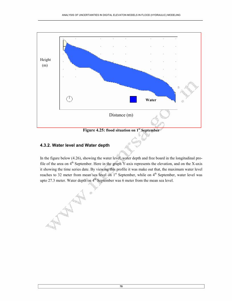
ANALYSIS OF UNCERTAINTIES IN DIGITAL ELEVATON MODELS IN FLOOD (HYDRAULIC) MODELING
70
Height
(m)
Distance (m)
Figure 4.25: flood situation on 1st September
4.3.2. Water level and Water depth
In the figure below (4.26), showing the water level, water depth and free board in the longitudinal pro-
file of the area on 4th September. Here in the graph Y-axis represents the elevation, and on the X-axis
it showing the time series date. By viewing this profile it was make out that, the maximum water level
reaches to 32 meter from mean sea level on 1st September, while on 4
th September, water level was
upto 27.3 meter. Water depth on 4th September was 6 meter from the mean sea level.
Water
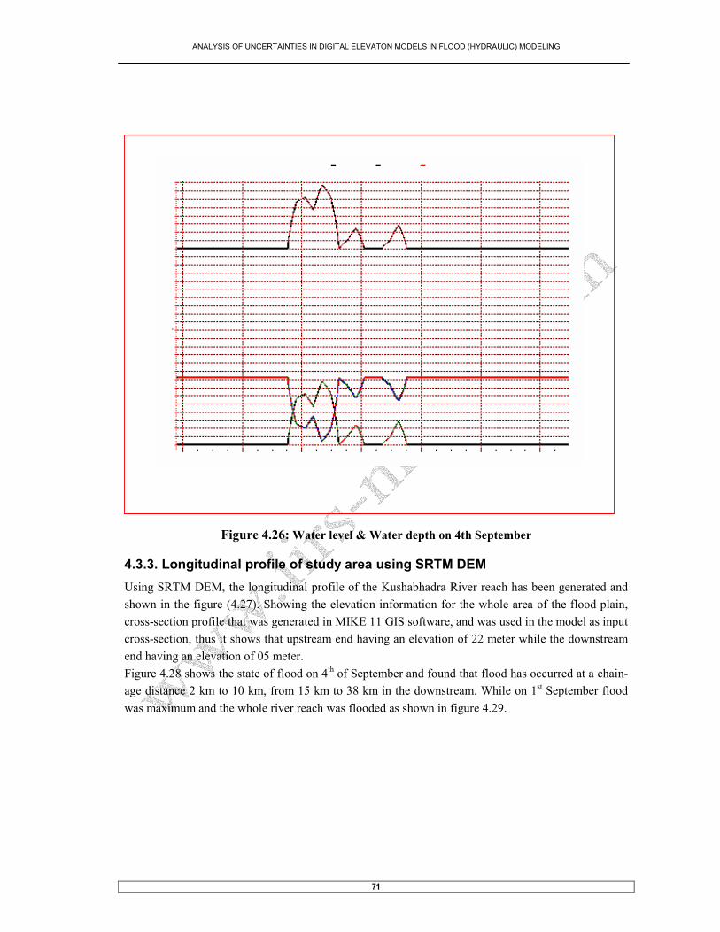
ANALYSIS OF UNCERTAINTIES IN DIGITAL ELEVATON MODELS IN FLOOD (HYDRAULIC) MODELING
71
Figure 4.26: Water level & Water depth on 4th September
4.3.3. Longitudinal profile of study area using SRTM DEM
Using SRTM DEM, the longitudinal profile of the Kushabhadra River reach has been generated and
shown in the figure (4.27). Showing the elevation information for the whole area of the flood plain,
cross-section profile that was generated in MIKE 11 GIS software, and was used in the model as input
cross-section, thus it shows that upstream end having an elevation of 22 meter while the downstream
end having an elevation of 05 meter.
Figure 4.28 shows the state of flood on 4th of September and found that flood has occurred at a chain-
age distance 2 km to 10 km, from 15 km to 38 km in the downstream. While on 1st September flood
was maximum and the whole river reach was flooded as shown in figure 4.29.

ANALYSIS OF UNCERTAINTIES IN DIGITAL ELEVATON MODELS IN FLOOD (HYDRAULIC) MODELING
72
Height
(m)
Distance (m)
Figure 4.27: Longitudinal profile of the study area
Maximum Water Level
Embankment Height
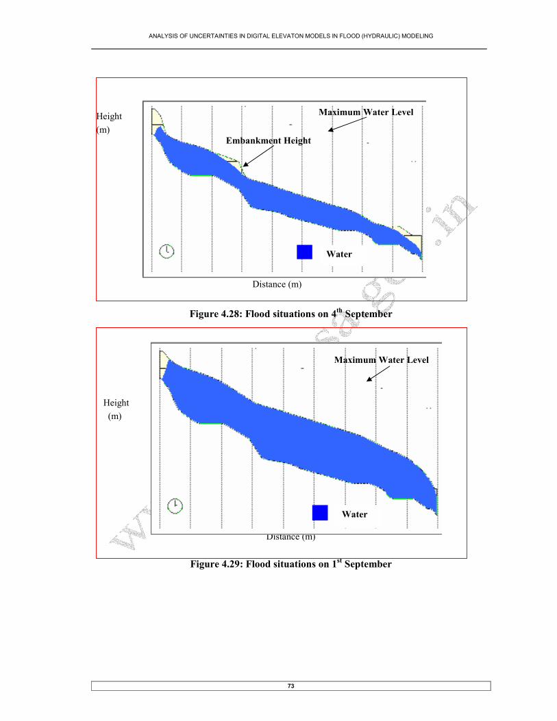
ANALYSIS OF UNCERTAINTIES IN DIGITAL ELEVATON MODELS IN FLOOD (HYDRAULIC) MODELING
73
Height
(m)
Distance (m)
Figure 4.28: Flood situations on 4th September
Height
(m)
Distance (m)
Figure 4.29: Flood situations on 1st September
Maximum Water Level
Water
Water
Maximum Water Level
Embankment Height
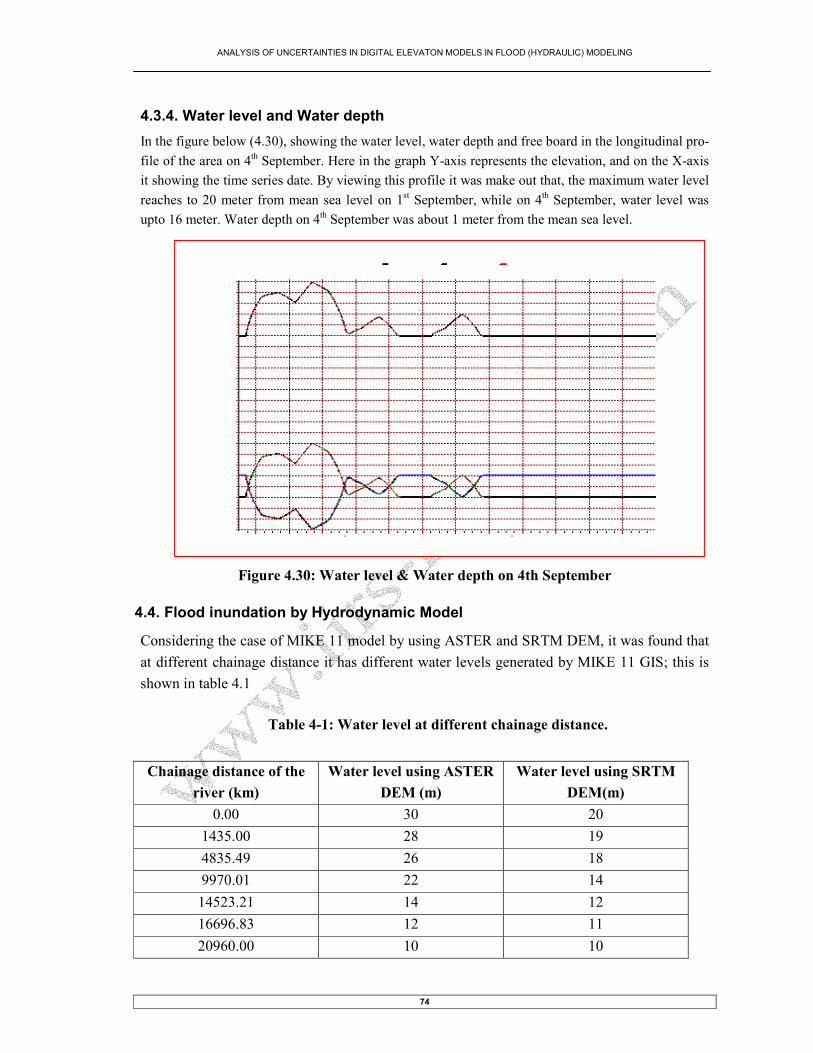
ANALYSIS OF UNCERTAINTIES IN DIGITAL ELEVATON MODELS IN FLOOD (HYDRAULIC) MODELING
74
4.3.4. Water level and Water depth
In the figure below (4.30), showing the water level, water depth and free board in the longitudinal pro-
file of the area on 4th September. Here in the graph Y-axis represents the elevation, and on the X-axis
it showing the time series date. By viewing this profile it was make out that, the maximum water level
reaches to 20 meter from mean sea level on 1st September, while on 4
th September, water level was
upto 16 meter. Water depth on 4th September was about 1 meter from the mean sea level.
Figure 4.30: Water level & Water depth on 4th September
4.4. Flood inundation by Hydrodynamic Model
Considering the case of MIKE 11 model by using ASTER and SRTM DEM, it was found that
at different chainage distance it has different water levels generated by MIKE 11 GIS; this is
shown in table 4.1
Table 4-1: Water level at different chainage distance.
Chainage distance of the
river (km)
Water level using ASTER
DEM (m)
Water level using SRTM
DEM(m)
0.00 30 20
1435.00 28 19
4835.49 26 18
9970.01 22 14
14523.21 14 12
16696.83 12 11
20960.00 10 10

ANALYSIS OF UNCERTAINTIES IN DIGITAL ELEVATON MODELS IN FLOOD (HYDRAULIC) MODELING
75
Flood inundation with respect to water level was generated in MIKE 11 model using ASTER DEM is
shown in figure 4.31
Figure 4.31: Flood inundation at different chainage distance(ASTER)
Water level >10m
Water level >12m
Water level >14m
Water level >22m
Water level >26m
Water level >28m
Water level >30m

ANALYSIS OF UNCERTAINTIES IN DIGITAL ELEVATON MODELS IN FLOOD (HYDRAULIC) MODELING
76
Water level >10 m
Water level >11m
Water level >12m
Water level >14m
Water level >18m
Water level >19m
Water level >20m
Flood inundation generated in MIKE 11 model using SRTM DEM is shown in figure 4.32
Figure 4.32: Flood inundation at different chainage distance(SRTM)
Area of flood inundation due to the different water level has been shown for ASTER and
SRTM in table 4.2 & 4.3 respectively.
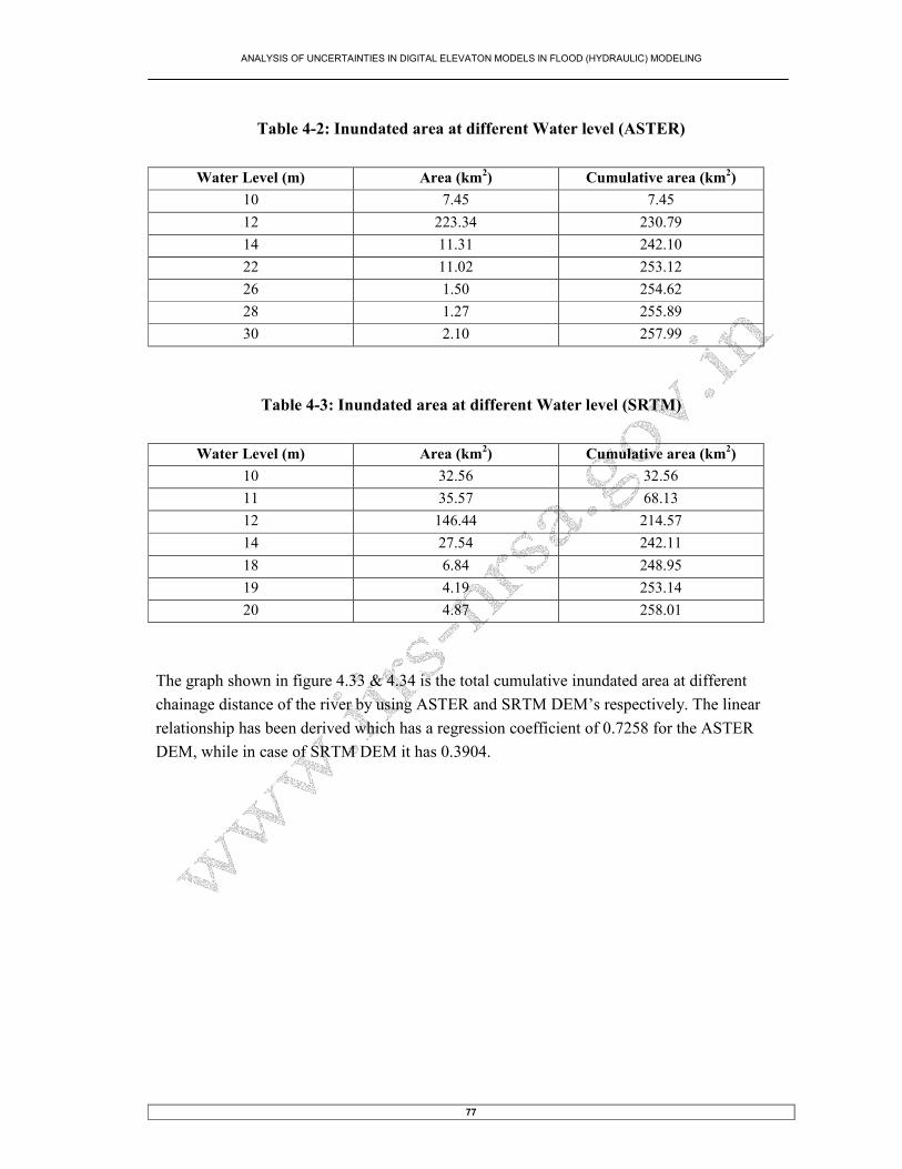
ANALYSIS OF UNCERTAINTIES IN DIGITAL ELEVATON MODELS IN FLOOD (HYDRAULIC) MODELING
77
Table 4-2: Inundated area at different Water level (ASTER)
Water Level (m) Area (km2) Cumulative area (km
2)
10 7.45 7.45
12 223.34 230.79
14 11.31 242.10
22 11.02 253.12
26 1.50 254.62
28 1.27 255.89
30 2.10 257.99
Table 4-3: Inundated area at different Water level (SRTM)
Water Level (m) Area (km2) Cumulative area (km
2)
10 32.56 32.56
11 35.57 68.13
12 146.44 214.57
14 27.54 242.11
18 6.84 248.95
19 4.19 253.14
20 4.87 258.01
The graph shown in figure 4.33 & 4.34 is the total cumulative inundated area at different
chainage distance of the river by using ASTER and SRTM DEM’s respectively. The linear
relationship has been derived which has a regression coefficient of 0.7258 for the ASTER
DEM, while in case of SRTM DEM it has 0.3904.

ANALYSIS OF UNCERTAINTIES IN DIGITAL ELEVATON MODELS IN FLOOD (HYDRAULIC) MODELING
78
Figure 4.33: Total cumulative inundated area at different chainage of the river(ASTER)
Figure 4.34: Total cumulative inundated area at different chainage of the river(SRTM)

ANALYSIS OF UNCERTAINTIES IN DIGITAL ELEVATON MODELS IN FLOOD (HYDRAULIC) MODELING
79
4.5. Uncertainty analysis
Digital Elevation Models (DEMs) are representations of topography with inherent errors that consti-
tute uncertainty. DEM data are often used in analyses without quantifying the effects of these errors.
Sources of possible error in DEM data sets include (Burrough, 1986; Wise, 1988):
• Data errors due to the age of data, incomplete density of observations or results of spatial
sampling.
• Measurement errors such as positional inaccuracy, data entry faults, or observer bias.
• Processing errors such as numerical errors in the computer, interpolation errors or classi-
fication and generalization problems
It is a practically impossible to obtain information on the exact source and quantity of error in a DEM.
Such an undertaking would involve, for example, field measurements over an approximate 55-square-
mile (35,766-acre) area. The area might be segmented into a grid of 900 square meters per grid total-
ling 144,801,000 grid cells within which one or more elevation readings might be measured. Even
such an undertaking, if physically possible, is subject to errors. The underlying assumption of this re-
search is that specific error within DEMs cannot be known and therefore the elevation model is re-
plete with uncertainty.
Different methods for representing error and quantifying uncertainty were investigated. Different
methods for uncertainty analysis available in the literature are given below. Uncertainty analysis was
calculated considering ASTER DEM as an base map
4.5.1 Root Mean Square Error (RMSE)
The RMSE is a commonly employed measure of estimator performance. The RMSE is used by to in-
dicate vertical accuracy of an entire grid. Here, the RMSE grid represents the expected accuracy of
each cell under the simulated uncertainty conditions. The RMSE is expressed as:
The RMSE was calculated as 14.70, while a valuable quality-control statistic, does not provide the
DEM user with an accurate assessment of how well each cell in the DEM represents the true eleva-
tion. It merely provides an assessment of how well the DEM corresponds to the data from which it
was generated. However, this statistic is often the only information DEM users have with which to
evaluate the quality of a particular DEM. The RMSE is valuable in that it can serve as a range for use
in simulation techniques. The true elevation can be expected to exist within the range provided by the
RMSE.

ANALYSIS OF UNCERTAINTIES IN DIGITAL ELEVATON MODELS IN FLOOD (HYDRAULIC) MODELING
80
4.5.2 Bias
Bias measures the average deviation of the statistic and is expressed as
Where refers to the estimator of the parameter and N is the number of simulations (i.e. N =
125). Bias was calculated as 13.55. Each cell in the bias grid represents the average amount of varia-
tion expected for that parameter at that particular location. For example, if the bias for column 1 row 1
in the elevation grid is 4, the elevation can be expected to vary, on average, +- 4.
4.5.3 Relative Bias
Relative Bias expresses the average percent deviation of the statistic from the original value and is
expressed as
Each value in the relative bias grid can be interpreted as the percent that location is expected to deviate
under the simulated uncertainty conditions. It was calculated as 17.75.

ANALYSIS OF UNCERTAINTIES IN DIGITAL ELEVATON MODELS IN FLOOD (HYDRAULIC) MODELING
81
5. Discussion and Conclusion
With the above and within the context, the study conducted on the flood event at the canal has thrown up
a lot of points worth considering, first and foremost of which are the-
Flood frequency analysis, which is the standard procedure to determine probability of flood flows, con-
sists of fitting the observed stream flow records to specify probability distributions. The data availability
to carry out flood frequency was not sufficient, only water level and discharge of Balianta station (gauzing
site) was available for five years and one year respectively, and the water level at the spillway was calcu-
lated by Central Water Commission, Bhubaneswar has been used. With the help of this the discharge was
estimated by deriving the relationship between water level and discharge. Power and Exponential relation-
ships has been used to determine the stage-discharge relationship, (shown in figure 2.1 and 2.2), Power
relationship was used as regression co-efficient was higher than that of Exponential relationship. Thus the
discharge that was calculated was used for the input discharge at the upstream of the canal.
Evaluation of the ability of RADAR and Optical remote sensing image time series data to detect flood
inundation in a river reach has been done, and has been found that Optical image does not throw suffi-
cient light to map of the flood extent, basically in India, flood occurs during monsoon period, as optical
image require cloud free condition, so it can be said that optical image was good for the land use/land
cover mapping, but for the flood interpretation from optical sensor (LISS III) can not be done due to the
obstruction in acquisition of image made by the cloud cover and also canopy cover, while RADARSAT
provides its own microwave illumination and thus will operate day and night, regardless of weather condi-
tions, the flood inundated mapping carried by temporal RADARSAT image (figure 2.4 (B) and figure 2.5
(A) and (B)) has been accurately delineated the spatial extent of flood as this was compared during the
field. Thus flood inundated map was prepared to make a comparison with the flood inundated scenario
generated by hydrodynamic models.
As the study area lies in the restricted zone, topographic map was not available, so digital elevation model
(DEM) could not be generated with the topographical map. Digital elevation model (DEM) from the pub-
lic domain which is available in internet is used in this study. Two DEMs that were used were ASTER
DEM and SRTM DEM. The minimum and maximum elevation in the study area for ASTER DEM was in
a range of 0 to 93 meters where as for SRTM DEM the maximum and minimum elevation in the study
area was in a range of 0 to 41 meters, these shows that for the same area there was big difference in ele-
vation information, it was difficult to quantify the amount of error, this shows the uncertainty in DEM.
Digital elevation models (DEMs) are representing the topographic elevation with some percentage of error
that constitute uncertainty. DEMs are key parameters for Hydrodynamic models but these DEMs data are
often used without quantifying the effect of this error. As the study area lies in restricted zone, spot height
data was not available. Comparison was made between ASTER and SRTM DEM considering ASTER
DEM as an base height, there were an wide range of differences in elevation information for the same spot
areas, it was found that for SRTM DEM the elevation can be expected to vary, about (+- )14 meters, In an
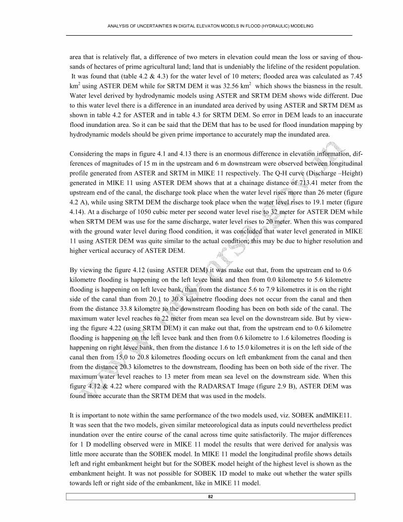
ANALYSIS OF UNCERTAINTIES IN DIGITAL ELEVATON MODELS IN FLOOD (HYDRAULIC) MODELING
82
area that is relatively flat, a difference of two meters in elevation could mean the loss or saving of thou-
sands of hectares of prime agricultural land; land that is undeniably the lifeline of the resident population.
It was found that (table 4.2 & 4.3) for the water level of 10 meters; flooded area was calculated as 7.45
km2 using ASTER DEM while for SRTM DEM it was 32.56 km
2 which shows the biasness in the result.
Water level derived by hydrodynamic models using ASTER and SRTM DEM shows wide different. Due
to this water level there is a difference in an inundated area derived by using ASTER and SRTM DEM as
shown in table 4.2 for ASTER and in table 4.3 for SRTM DEM. So error in DEM leads to an inaccurate
flood inundation area. So it can be said that the DEM that has to be used for flood inundation mapping by
hydrodynamic models should be given prime importance to accurately map the inundated area.
Considering the maps in figure 4.1 and 4.13 there is an enormous difference in elevation information, dif-
ferences of magnitudes of 15 m in the upstream and 6 m downstream were observed between longitudinal
profile generated from ASTER and SRTM in MIKE 11 respectively. The Q-H curve (Discharge –Height)
generated in MIKE 11 using ASTER DEM shows that at a chainage distance of 713.41 meter from the
upstream end of the canal, the discharge took place when the water level rises more than 26 meter (figure
4.2 A), while using SRTM DEM the discharge took place when the water level rises to 19.1 meter (figure
4.14). At a discharge of 1050 cubic meter per second water level rise to 32 meter for ASTER DEM while
when SRTM DEM was use for the same discharge, water level rises to 20 meter. When this was compared
with the ground water level during flood condition, it was concluded that water level generated in MIKE
11 using ASTER DEM was quite similar to the actual condition; this may be due to higher resolution and
higher vertical accuracy of ASTER DEM.
By viewing the figure 4.12 (using ASTER DEM) it was make out that, from the upstream end to 0.6
kilometre flooding is happening on the left levee bank and then from 0.0 kilometre to 5.6 kilometre
flooding is happening on left levee bank, than from the distance 5.6 to 7.9 kilometres it is on the right
side of the canal than from 20.1 to 30.8 kilometre flooding does not occur from the canal and then
from the distance 33.8 kilometre to the downstream flooding has been on both side of the canal. The
maximum water level reaches to 22 meter from mean sea level on the downstream side. But by view-
ing the figure 4.22 (using SRTM DEM) it can make out that, from the upstream end to 0.6 kilometre
flooding is happening on the left levee bank and then from 0.6 kilometre to 1.6 kilometres flooding is
happening on right levee bank, then from the distance 1.6 to 15.0 kilometres it is on the left side of the
canal then from 15.0 to 20.8 kilometres flooding occurs on left embankment from the canal and then
from the distance 20.3 kilometres to the downstream, flooding has been on both side of the river. The
maximum water level reaches to 13 meter from mean sea level on the downstream side. When this
figure 4.12 & 4.22 where compared with the RADARSAT Image (figure 2.9 B), ASTER DEM was
found more accurate than the SRTM DEM that was used in the models.
It is important to note within the same performance of the two models used, viz. SOBEK andMIKE11.
It was seen that the two models, given similar meteorological data as inputs could nevertheless predict
inundation over the entire course of the canal across time quite satisfactorily. The major differences
for 1 D modelling observed were in MIKE 11 model the results that were derived for analysis was
little more accurate than the SOBEK model. In MIKE 11 model the longitudinal profile shows details
left and right embankment height but for the SOBEK model height of the highest level is shown as the
embankment height. It was not possible for SOBEK 1D model to make out whether the water spills
towards left or right side of the embankment, like in MIKE 11 model.

ANALYSIS OF UNCERTAINTIES IN DIGITAL ELEVATON MODELS IN FLOOD (HYDRAULIC) MODELING
83
The differences can be attributed to a variety of reasons ranging from the algorithms used to the
method of data collection. It is also important to note that expectations of good performance of all
models over all types of terrain and geophysical conditions can be no more than wishful thinking. It
can still be said with considerable satisfaction from the result derived; that for 1D modeling the DEM
derived from ASTER and the MIKE 11 model would be the best bet should simulations of a similar
kind be carried out in the region armed with more detailed data. An 2 D modelling was also been tried
in SOBEK model to generate an flood inundation map, but had not been possible, the problem that has
been faced was, after flow and data view model has been checked , then in pre-processing it shows
run-time error message this may be due to the greater size of DEM, i.e handling of large amount of
data.
It can be thus concluded that the study, while lacking in substantial confidence due to inherent incon-
sistencies of data related to real-time flood level measurements along short chainage, the density both
spatial and temporal of measurements of precipitation, and depth of information with respect to accu-
rately measured and densified network of control points, was successful in its primary objective. The
DEM that should be used would contain acceptable error for mapping of flood inundated area accu-
rately. The simulation and the associated field study also bring to question the worth of building em-
bankments on rivers or in other words the efficiency of structural measures over non-structural meas-
ures such as catchments treatment and watershed management. Although the study did not incorporate
a review of the methods of damage assessment in such conditions and/or the methodologies to be fol-
lowed for the mitigation and control, it is observed that inclusion of the above said aspects would con-
siderably strengthen the value.
A lot has been said but much less done of the state of affairs of disaster management scenario in India.
The recent Tsunami impact in the eastern coast will surely bring to front new paradigms to the facets
of disaster prediction, impact assessment and mitigation in the light of comparisons with the perform-
ance of earthquake rehabilitation programmes in Gujarat. As has been mentioned earlier, natural dis-
asters compare as strongly with respect to the devastation they wreak to their unpredictability of oc-
currences, and thus warranting all attempts of simulations for risk assessment justified.
Finally, Should the data as mentioned here and reported elsewhere in the study be generated and made
freely available, such simulations would give a deeper insight into the dynamics of flood events, and
extended to other domains, the entire gamut of disasters that the nation faces on this date.

ANALYSIS OF UNCERTAINTIES IN DIGITAL ELEVATON MODELS IN FLOOD (HYDRAULIC) MODELING
84
References:
Adam, S. Wiebe, J. Collins, M. and Pietroniro, A., (1998): Radarsat flood mapping in the Peace-
Athabasca Delta, CanadaCanadian Journal of Remote Sensing 24(1), pp 69-79.
Archer, D., (1999): Practical application of historical flood information to flood estimation, In; Got-
tchalk L., Olivry J.C., Reed D., Rosjberg D., Hydrological Extremes: Understanding, Predicting, Miti-
gating, IAHS Pub. No. 255, pp 209-215.
Bates, P.D., Roo, A.P.J., (2000): A simple raster based model for flood inundation simulation, Journal
of Hydrology, 236, pp 54-77.
Bates, P. D. S., Horritt, C. N. Smith and Mason. D., (1997). Integrating remote sensing observations
of flood Hydrology and hydraulic modeling. Hydrological processes, vol. 11, pp 1777-1795.
Beven, K.J., (1989): Changing ideas in hydrology: The case of physically based models. J. Hydrol.
105, pp 157–172.
Birkett, C.M., (2000): Synergetic remote sensing of lake chad; variability of basin Inundation, Remote
Sensing of Environment 72, pp 218-236
Black A.R. and Burns J.C., (2002): Re-assessing flood risk in Scotland, Science of the total environ-
ment, 294: pp 169-184.
Bronstert, A., Menzel, L., (2002): Advances in flood research, Journal of Hydrology 267.
Burrough, P. and McDonnell, R., (1998): Principles of Geographic Information Systems, Oxford Uni-
versity Press, New York, NY, pp 333
Byrne, G.F., Crapper, P.F.,Mayo,K.K., (1980): Monitoring land-cover change by principal component
analysis of multitemporal Landsat data.Remote Sensing of Environment 10, pp 175-184.
Colditz, R.R., (2003): Land cover and geomorphological floodplain mapping of the lower Panuco ba-
sin. Mexico, utilizing remote sensing and GIS-methods.Diplomarbeit, Bayerische Julius-Maimilians-
Universitat Wurzburg, Germany, unpublished, pp 197.
Colvocoresses, A.P., (1982): An automated mapping satellite system (Mapsat). Photogrammetric En-
gineering and Remote Sensing 48 (10), pp 1585– 1591.
Disaster Mitigation & Vulnerability Atlas of India, URL (http://www.bmtpc.org/disaster.htm), Ac-
cess on 27 September 2004.
ESRI, (1996): Arc View Spatial Analyst, Environmental Systems Research Institute, Inc., Redlands,
pp 147.
Frazier, P.S., Page, K.J., (2000): Water body detection and delineation with Landsat TM data, Photo-
grammetric Engineering and Remote Sensing 66, pp 1461-1467.
Fujisada, H., (1994): Overview of ASTER instrument on EOS-AM1 platform. Proceedings of SPIE,
vol. 2268. The International Society for Optical Engineering, pp 14– 36.
Galy H. & Sanders R.A., (1998): Flood modelling using air borne synthetic aperature radar data,
london.

ANALYSIS OF UNCERTAINTIES IN DIGITAL ELEVATON MODELS IN FLOOD (HYDRAULIC) MODELING
85
Honda, Kiyoshhi, Francis X.J Cannisius and Bhuwneshwar Prasad Sah (1997): Flood monitoring in
Central Plane of Thailand Using JERS-1 SAR Data” Proceedings of GIS development.
Hunter, G. and Goodchild, M., (1997): Modeling the Uncertainty of Slope and Aspect Estimates De-
rived From Spatial Databases, Geographical Analysis, Vol. 29, No. 1, pp 35-49.
InfoChange manage-disaster. Pune, InfoChange A-3, Silver Spurs NIBM Road
Kondwa, Pune-411048
India Tel: 91-20-685 4062/684 2845 E-mail: [email protected]. 2004.
Jothityangkoon, C., Sivapalan, M. and Farmer, D.L., (2001): Process controls of water balance vari-
abiity in a large semi-arid catchments: downward approach to hydrological model development. Jour-
nal of Hydrology 254, pp 174–198.
Katayama, T., (1994): International Decade for Natural Disaster Reduction: Working Against Time.
UNU University Lectures. The United Nations University. Tokyo.
Knighton, D., (1998): Fluvial forms and processes, Arnold, London, pp 383.
Leavesley, G.H., (1994): Modeling the effects of climate change on water resources—a review. Cli-
matic Change 28, pp 159–177.
Leavesley, G.H., Litchy, R.W., Troutman, B.M. and Saindon, L.G., (1983): Precipitation-Runoff
Modeling System: User's Manual. US Geological Survey Water Resources Investigative Report, Den-
ver, Colorado, pp 83–4238.
Mertes, L.A.K., (1995): Rates of Flood Plain Sedimentation on the Central Amazon River, Geology,
22, pp 171-174.
Moffatt and Nichol engineers, (2003): South Bay Salt Pond Restoration Project: Hydrodynamic Mod-
eling tools and Techniques, Prepared For: California state coastal conservancy, 1330 Broadway, Ste
1100 Oakland, CA 94612.
Monckton, C., (1994): An investigation into the spatial structure of error in digital elevation data, In:
Innovations in GIS Volume 1, pub-M.Worrboys, Taylor and Francis, Bristol, pp-267.
Moore, I.D., Grayson, R.B. and Ladson, A.R., (1991): Digital terrain modeling: a review of hydro-
logical, geomorphological, and biological applications. Hydrological Processes 5, pp 3–30.
Ormsby, J.P. and Blanchard B. J., (1985): Detection of Lowland Flooding using Active Microwave
Systems, Photogram. Eng. And Rem. Sens. 51(3): pp 317-328.
Philip A, Townsend, Stephen J. Walsh, (1998): Modeling floodplain inundation using an integrated
GIS with radar and optical remote sensing. Geomorphology 21: pp 295-312
Pietroniro, A., Prowse, T.D., (2000): Preface: application of remote sensing in hydrology. Hydrologi-
cal processes 16, pp 1537-1541.
Plate E.J., (2002): Flood risk and flood management. Journal of Hydrology 267, pp 2-11
Poole, G.C., Stanford, J.A., Frissell, C.A., Running, S.W., (2002): Three-dimensional mapping of geo-
morphic controls on flood plain hydrology and connectivity from aerial photos. Geomorphology 48,
pp 329-347

ANALYSIS OF UNCERTAINTIES IN DIGITAL ELEVATON MODELS IN FLOOD (HYDRAULIC) MODELING
86
Pultz T.J. and Y. Crevier., (1997): Early Demonstrations of RADARSAT for Application in Hydrol-
ogy, In: G.W. Kite, A. Pietroniro and T. Pultz (eds) (1996): Application of Remote Sensing in Hy-
drology, Third International Workshop, Goddard Space Flight Centre, Washington, D.C., USA,
Refsgaard, J.C., (1987). A methodology for distinguishing between the effects of human influence and
climate variability on the hydrologic cycle. Proceedings of the Vancouver Symposium ‘The Influence
of Climate Change Variability on the Hydrologic Regime and Water Resources’, August 1987. IAHS,
Published. no. 168, Vancouver, pp 557–570.
Rango, A. and A.T. Anderson., (1974): Flood Hazard Studies in the Mississipi River Basin using Re-
mote Sensing, Water Resource. Bull., vol 10, pp 1060-1081.
Sabins, F.F., (1997): Principles and interpretation, W.H.Freeman and company , New York.
Seth, S.M., (1998): Flood Hydrology and Flood Management in India, in Flood Studies in India eds.
Kale, Vishwas S. (1998), Geological Society of India, Bangalore.
Shafiee, Mardiana, Azman Ahmad and Osman Kadir., (2000): “Capability of Radarsat Data in Mon-
soon Flood Monitoring”, ACRS 2000, GISdevelopment.net
Smith, L.C., (1997): Satellite remote sensing of river inundation area, stage and discharge: a review.
Hydrological Processes 11, pp 1427- 1439.
Sorensen, H.R., Kjelds, J., Deckers, F., Waardenburg, F., (1996): Application of GIS in hydrological
and hydraulic modelling, DLIS and MIKE 11-GIS, HydroGIS 96, DHI reference, 1996/09.
Srivastava, Y.K., Binod Doley, D.K. Pal., R.K. Das., S. Sudhakar., S. Adiga., K.V. Venkatachary.,
S.K. Srivastava., (2000): High Resolution Remote Sensing Data & GIS Techniques in Updation of
Infrastructure Details for Flood Damage Assessment - A Case Study, Proceedings of GIS develop-
ment.
Struve, H., and Judson, F.E., (1979) "Development of Stage Area Tables for the Yazoo Backwater
Area Using Landsat Data" in Proceedings of the U.S. Army Corps of Engineers Remote Sensing Sym-
posium, pp 193-199
Thompson, L.G., (2000). Ice core evidence for climate change in the tropics, implications for our fu-
ture, Quaternary Science Reviews 19, pp 19-35.
Townsend, Philip A. and Jane R. Foster., (2002): “Assessing Flooding and Vegetation Structure in
Forested Wetlands using Radarsat SAR Imagery” Proceedings of the 2002 International Geosciences
and Remote Sensing Symposium. Toronto Canada, June 24-28.
Toyra, J., Pietroniro, A., Martz, L.W., Prowse, T.D., (2002): A multi-sensor approach to wetland
flood monitoring. Hydrological Processes 16, pp 1569-1581.
United States Geological Survey., (1997): Standards For Digital Elevation Models, Department of the
Interior, Washington, DC.
URL1, Organigation of American state, http://www.oas.org/usde/publications/Unit/oea66e/ch08.htm
Wang, Y., L.L. Hess. S. Filoso and J.M. Melack., (1995): Understanding the Radar Backscattering
from Flooded and Non-flooded Amazonian Forests: Results from Canopy Backscatter Modeling, Re-
mote Sens. Environ. 54, pp 324-332.

ANALYSIS OF UNCERTAINTIES IN DIGITAL ELEVATON MODELS IN FLOOD (HYDRAULIC) MODELING
87
Williams A., and Archer D., (2002,): The use of historical flood information in the English midlands
to improve risk assessment, Hydrological Science Journal, 47(1): pp 67-76.
Wood, J., (1996): The Geomorphological Characterization of Digital Elevation Models, Ph.D. Disser-
tation, Department of Geography, University of Leicester, Leicester, UK,
Yamagata. Y., Akiyama. T., (1988): Flood damage analysis using multi-temporal Landsat Thematic
Mapper data. International Journal of Remote Sensing 9, pp 503-514.