accelerated time-of-flight mass spectrometry - arxiv · accelerated time-of-flight mass...
TRANSCRIPT

1
Accelerated Time-of-Flight Mass SpectrometryMorteza Ibrahimi, Student Member, IEEE, Andrea Montanari, Senior Member, IEEE,
and George Moore, Senior Member, IEEE
Abstract—We study a simple modification to the conventionaltime of flight mass spectrometry (TOFMS) where a variable and(pseudo)-random pulsing rate is used which allows for tracesfrom different pulses to overlap. This modification requireslittle alteration to the currently employed hardware. However,it requires a reconstruction method to recover the spectrumfrom highly aliased traces. We propose and demonstrate anefficient algorithm that can process massive TOFMS data usingcomputational resources that can be considered modest withtoday’s standards. This approach can be used to improve dutycycle, speed, and mass resolving power of TOFMS at the sametime. We expect this to extend the applicability of TOFMS tonew domains.
Index Terms—Time of flight mass spectrometry.
I. INTRODUCTION
Mass spectrometry (MS) refers to a family of techniquesused to analyze the constituent chemical species in a sample.The applications abound in science and technology and newfields of scientific investigations have evolved around thesetechniques. An example is proteomics which refers to thescience of analyzing peptides and proteins. Proteins are theworkhorse of many biological mechanism. Of great interest tobiological sciences, medical research and drug discovery anddevelopments is identifying and analyzing the composition andstructure of proteins and other large chemical compounds. Ithas become possible only recently to analyze the compositionof proteins with high throughput and accuracy through massspectrometry techniques [1] [2]. Other applications includemeasuring isotopic ratio, space exploration, testing for illegalsubstances etc. Mass spectrometers are usually accompaniedwith gas or liquid chromatography techniques and are used indifferent configurations in tandem with other mass spectrome-ter of the same or different types. These configurations providea wide range of utility and performance criteria making massspectrometry relevant for many different applications.
A typical mass spectrometer consists of three main modules:an ionizer, a mass analyzer, and a detector. The ionizer con-verts the species of interest, and possibly other compounds inthe sample to ions in gas phase. Recent advances in ionizationtechniques, namely matrix assisted laser desorption ionization[3], and electrospray ionization [2] has made it possible toionize and transform into gas phase large intact moleculeslike proteins. These techniques provided new applications formass spectrometry and open new avenues for analyzing thecomposition and structure of proteins [4].
M. Ibrahimi is with the Department of Electrical Engineering, StanfordUniversity, Stanford, CA, 94305 USA email: [email protected].
A. Montanari is with the Department of Electrical Engineering and De-partment of Statistics, Stanford University, Stanford, CA, 94305 USA email:[email protected].
Fig. 1: Different parts of a TOFMS.
The purpose of the mass analyzer module is to separate theions according to their mass to charge ratio (MCR). Today’scommon mass analyzers separate the ions by subjecting themto electromagnetic fields. These fields exert different forcesto different ions. One class of instruments, broadly referredto as sector instruments cause the ions with different MCR totake different trajectories, effectively beamforming a stream offlying ions of particular MCR toward a detector [5] Anothertechnique is to have all the ions travel a common trajectorybut with different velocities. This is the basis for time of flight(TOF) mass spectrometers which we shall describe throughlyin the sequel. A third approach is to guide only a particularMCR to have a stable trajectory. This is the basis for theQuadrupole and ion trap mass analyzers [6]. These instrumentscan act as a MCR filter or scan a wider range by sweepingthe filter pass band.
The detector module senses the ions by detecting the impactof charged compounds with the detector surface or the chargeor current they induce by their particular motion.
In this paper we are concerned with time of flight massspectrometry (TOFMS) which is a simple yet powerful MStechnique. TOFMS was introduced in the 1940s by Stephens[7]. TOFMS offers two major benefits over alternative tech-niques. It has essentially unlimited mass range and highrepetition rate. These properties along with the recent advancesin available hardware and ionization techniques have madeTOFMS an appealing choice for the analysis of samples withwide mass range [8], biological macromolecules [9] and incombination with other mass spectrometers [10].
A basic TOF mass spectrometer consists of four parts: anionization chamber, an acceleration chamber, a drift region,and a detector (c.f., Fig 1). The sample is ionized in theionization chamber. These ions are then subjected to a verystrong electrical field in the acceleration chamber, effectivelyfiring them into the drift region. Ideally, the ions entering thedrift region have kinetic energy, K, proportional to their chargez, i.e., if the potential difference in the acceleration chamber isU then the following holds K = Uz. This means that an ionwith mass m has velocity v =
√2Uzm . Therefore, assuming
arX
iv:1
212.
4269
v2 [
mat
h.O
C]
28
Jul 2
013
2
that the length of the drift region to be L, the time to reachthe detector is
t =
√m
2z
L
2U. (1)
In other words, the time that takes for an ion to reach thedetector is proportional to
√m/z where m is the mass of the
ion and z is its net charge.TOFMS is a pulsed technique, i.e., ions are formed in an
ionization stage and subsequently accelerated as a packet intothe drift region with ions with different MCR traveling atdifferent speeds. As the ions impact the detector, they generatea continuous electrical signal which is then sampled resultingin a discrete signal. The result of this process, which wecall a scan, is a noisy sample of the
√m/z spectrum. A
single scan is often too noisy and this process is repeatedfrom hundreds to a few thousands times and averaged toobtain an accurate estimate of the
√m/z spectrum. We will
call an estimate of√m/z, which is the result of processing
many scans, one acquisition. In many applications multipleconsecutive acquisitions are obtained: to construct a movieof an evolving sample like an ongoing chemical reaction;to analyze the output of a preceding chromatography stage;or to mass analyze samples through an automated systemwhere TOFMS instrument in being fed automatically, e.g., inpharmaceutical applications [11].
There are several metrics that describe the performanceof a mass spectrometer. Some of the widely used metricsare: mass resolving power, mass accuracy, dynamic range,sensitivity and speed. Mass resolving power is the minimumdifference in mass to charge ratio for two present species tobe distinguishable by the instrument. Mass accuracy is thenormalized precision with which the instrument can report theMCR of present species, measured in MCR error divided byMCR. Mass range refers to the range of MCRs the instrumentcan detect. Sensitivity is the minimum concentration of anspecie to be detectable by the instruments. Finally, speed isthe number of acquisition the instrument can acquire per unittime.
These metrics are not independent. Several trade offs existamong these metrics based on how a TOFMS instrument isdesigned and operated. For example, speed can be increased,at the cost of mass resolving power, mass accuracy andsensitivity, by decreasing the number of scans collected foreach acquisition. Another trade off exists between speed inone hand and mass resolving power and accuracy on the otherhand, which is the focus of this paper and is described indetails below.
In conventional TOFMS, the time between consecutivepulses is set to be long enough to avoid overlap betweendifferent scans, i.e., for the slowest ion in an scan to arriveat the detector before the fastest ion of the next scan. Hence,acquisition time is lower bounded by,
Tacquisition ≥ N × T ∗scan
≥ N × L√2U
(√
(m/z)max −√
(m/z)min), (2)
where N is the number of scans collected for each acquisition.
Furthermore, the difference in time of arrival for two ions is
t2 − t1 =L√2U
(√m2/z2 −
√m1/z1). (3)
Hence, increasing the length of the drift region L (i)increases the acquisition time and therefore decreases thespeed (ii) spreads the ions further apart and therefore increasesthe mass accuracy and resoling power. This issue is of funda-mental importance because of the following.
Other factors that can improve the mass accuracy andresolving power of a TOFMS, e.g., detector characteristics andthe speed of the electronics, have reached their limits whilenew applications demand even better performance in terms ofmass accuracy and resolving power. One option that remainsavailable for improving the mass accuracy and resolving poweris to increase the length of the drift region.
However, first, there is the obvious desire for higher speedand accuracy at the same time. Second, some applications havestringent requirements in terms of speed, mass accuracy, re-solving power and sensitivity. This could be due to exogenoustime restrictions, e.g., when monitoring a chemical reactionor experimentation choice, e.g., when TOFMS is precededby a chromatography stage or used in tandem, with anothermass spectrometry stage. There is also significant economicalimplications, a high end instrument costs at the order ofhundreds of thousands of dollars and improving the speedand throughput while keeping or improving the accuracy canresult in significant savings. This is most clear in the case oflarge scale automated experiments used in drug discovery anddevelopment activities.
Therefore, simultaneous improvement of the speed and massaccuracy and resolving power is of fundamental interest inTOFMS [12].
Conventional TOFMS works by repeating the same exper-iment multiple times and averaging the results. The choice ofaveraging was mainly due to its simplicity.
In particular, the volume and rate of data generated byTOFMS instruments prohibited the use of more sophisticatedtechniques. Our ability to commit more computational re-sources has increased significantly since the introduction ofTOFMS. At the same time, the data rate of these instrumentsgenerate has also dramatically increased. In this paper, wepresent an efficient, highly parallelizable algorithm that inconjunction with a simple modification to the conventionalTOFMS can improve mass accuracy, mass resolving powerand speed at the same time.
There has been previous work trying to alleviate thisproblem. One approach, called Fourier transform TOF, isto modulate a continuous ion beam at the source using aperiodic waveform and subsequently accelerate it into the driftregion [13]. The detected signal is then demodulated to obtainthe spectrum. Another approach, called Hadamard transformTOF (HT-TOF) [14], is based on modulation (gating) of acontinuous ion source by a 0/1 pulse. In this approach, anion beam is deflected according to a pseudorandom sequenceof pulses. If the pulse is 1, the beam is undeflected and willreach the detector. In contrast, if the pulse is 0 the beam isdeflected away from the detector. The pulse sequence has the
3
same frequency as the detector. In an ideal case where thereis neither shot noise nor additive noise, the output can bedescribed as
y = Hx, (4)
where y ∈ Rn is the observed signal at the detector andx ∈ Rn is the TOF spectrum. H ∈ Rn×n is a 0/1 matrixwhere each column is the pseudorandom sequence shiftedby the index of the column. As long as H is full rank andthe model is accurate the TOF spectrum can be recovered byapplying the inverse of H to y. The spectrum is obtained bya deconvolution that can be implemented efficiently using thefast Hadamard transform.
One drawback of these methods is that they treat thereconstruction process as a deterministic inversion problemand ignore the noisy nature of the observations. Furthermore,they require substantial modification to the hardware of aconventional TOFMS. In this paper, we describe a differentmethod, called accelerated time of flight mass spectrometry(ATOF), which simultaneously achieves mass resolving power,duty cycle, and speed improvement using essentially thesame hardware as a conventional TOFMS. Our reconstructionscheme acknowledges the stochastic nature of the observation.Simulation results using real data confirm the performanceimprovement of this scheme.Notations and Terminology: Let [n] = {1, 2, . . . , n} and{x[i]}i=[n] be the output of the detector for a single scan.With a slight abuse of notation we also refer to x as ascan. Typically a TOFMS experiment consists of many scanswhich are later processed (simply averaged) to obtain a moreaccurate estimate of the spectrum. Let x(l)[i] be the lth scan.Define the true spectrum, x[i], as the average of infinitelymany scans, i.e., x[i] = limN→∞ 1
N
∑Nl=1 x
(l)[i]. Each scanx(l)[i] is therefore a noisy version of x[i]. We define the trace,y[t], t = 1, . . . T , to be the observed detector response formultiple, possibly overlapping scan. Given an observed tracey, the goal is to find a good estimate x of x.
In what follows we treat the discrete signals as columnvectors. For u and v two vector of the same dimension, let v∗
denote the transpose of v and 〈u, v〉 the scaler product of uand v.
As a matter of convention we refer to each element ofthe vectors that represent the spectrum (x(l) and x) as a binand to that of the trace as a sample, e.g., y[1] represents thefirst sample of the trace. When an ion impacts the detectorit generates a bell-shaped pulse in the output of the detector.We refer to an observed pulse in the trace as an impact event,or event for short. Usually the sampling rate of the detectorresponse is such that an event spans multiple samples.
For pedagogical reasons, we first describe the algorithm asif each event could occupy only one sample and there was notime jitter, i.e., all the ions of the same species are associatedwith the same bin. We then describe the algorithm without thisassumptions with some minor modifications. All the resultspresented in this paper are obtained using real data from aconventional TOFMS instrument which is used to simulatethe output of an ATOFMS. The algorithm used to obtain theseresults is the generalized version of the algorithm.
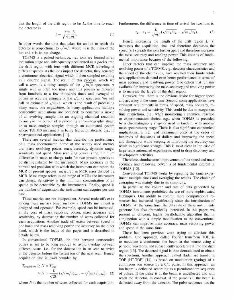
Fig. 2: Difference between TOFMS and ATOFMS. InATOFMS different scans can overlap resulting in shorteracquisition time for the same number of scans but also aconvoluted observed trace.
II. MEASUREMENT SCHEME AND THE DATA MODEL
A TOF measurement from a single scan is commonly verysparse (after removing the additive electrical noise throughpreprocessing, c.f. Section IV). Furthermore, a single mea-surement of the whole spectrum is not expensive and it canbe viewed as being performed in parallel as all ions are flyingin the drift region at the same time. However, the observedsignal from a single scan is too noisy and many repetitionsof the same measurement are necessary to obtain an accurateestimate of the spectrum. In a conventional TOFMS setting,the observed trace can be expressed as y[t] =
∑Nl=1 x
(l)[t−ln]where x(l) is the detector response to the lth scan and x[i] isunderstood to be zero for i ≤ 0 or i > n.
We incorporate a simple, yet powerful, modification to thisscheme [15] (c.f. Fig. 2). Conventional TOF (TOF) requirescollection of many scans, each scan collected independentlywith no overlap. ATOF idea is to increase the repetition rateand allow the subsequent scans to overlap.
Define τl, the firing time, to be the starting time of thelth scan, i.e., the time when the lth ion packet is acceleratedinto the drift region. Define ∆τl ≡ τl+1 − τl. In TOF ∆τl =∆τ ≥ n to avoid overlapping between consecutive scans. Werelax this condition and let ∆τl be a random variable withE[∆τl] = αn, for some α < 1. As is the case with the HT-TOF we assume that the detector response to overlapping scansis the superposition of the individual responses,
y[t] =
N∑l=1
x(l)[t− τl]. (5)
In this case at each time t, y[t] is the superposition of multipleoverlapping scans. Assume there are a total of N scans andlet 0 = τ1 < τ2 < · · · < τN be the firing times. For a givenτ = (τ1, τ2, . . . , τN ), define the matrix A ∈ RT×n as
A(t, i) =
{1 if ∃ l ∈ [N ] s.t. i = t− τl0 Otherwise. (6)
The matrix A can be considered as the adjacency matrix of abipartite graph (c.f., Fig 3), with rows of A corresponding tothe samples in the trace y and columns of A correspondingto the bins on the spectrum x. Sample t on the spectrum isconnected to bin i on the spectrum, i.e., Ati = 1, if and onlyif for some scan l ∈ [T ] the ions from bin i of the scan x(l)
arrive at time t in the trace y. In what follows, we will refer
4
0 n
T0
t
i i i1 2 3
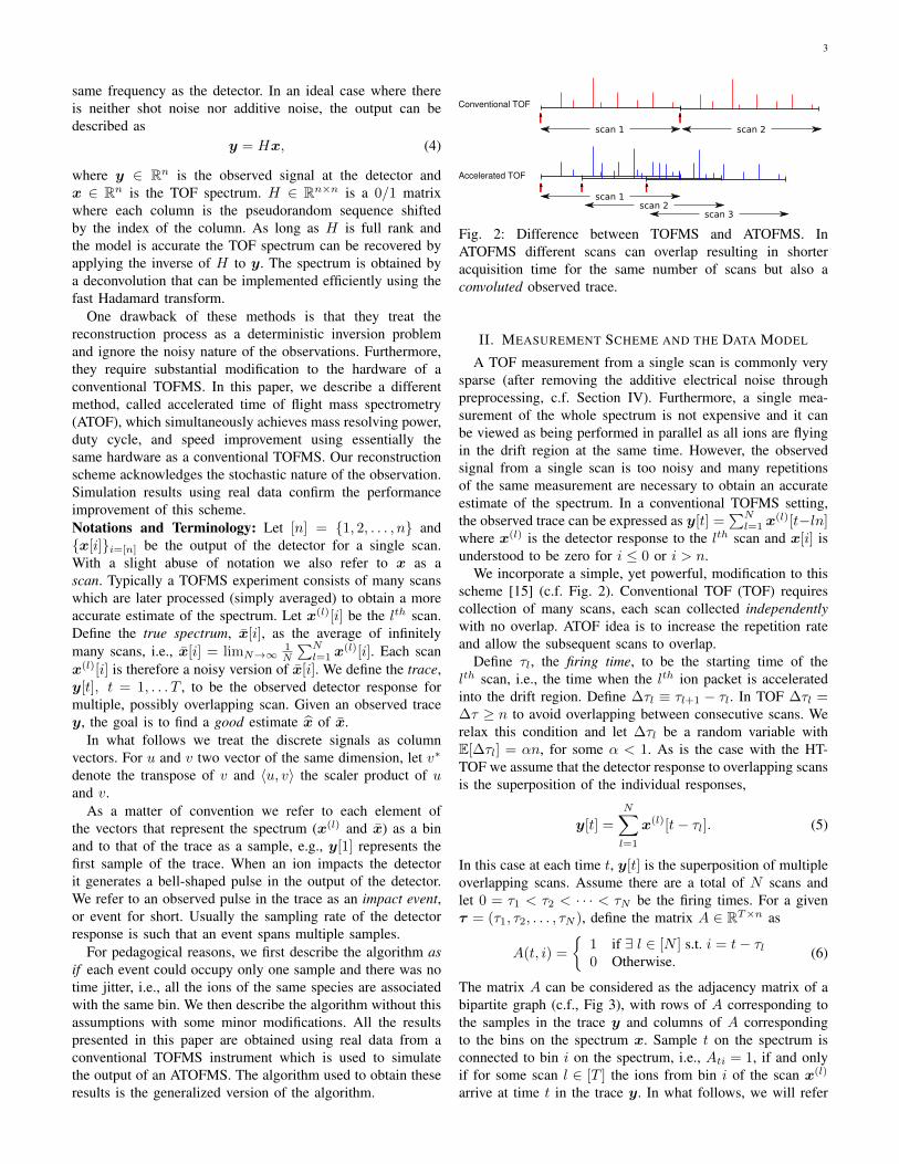
Fig. 3: Adjacency matrix A and the corresponding bipartitegraph. The signal on the top represents the spectrum and thebottom signal represents the trace. The trace is the overlappedconcatenation of noisy copies of the spectrum. Nodes are colorcoded where blue correspond to the first scan, purple to thesecond, and green to the third. Neighbors of sample t on thetrace are those bins on the spectrum who could potentiallycontribute to an event at sample t (again color coded).
to the neighbors of sample t as ∂t = {i ∈ [n] | A(t, i) > 0},and similarly to the neighbors of bin i as ∂i.y[t] can be considered as a noisy version of linear measure-
ments of x, 〈At, x〉, with At the tth row of A as a columnvector. In this notation, the TOF is a special case where eachrow of A has only one nonzero element, i.e., measurementy[t] corresponds to a noisy observation of x[i] for some bini. The structure of matrix A reveals the difference betweenATOF and TOF.
ATOF =
1 0 0 00 1 0 00 0 1 00 0 0 11 0 0 00 1 0 00 0 1 00 0 0 11 0 0 00 1 0 00 0 1 00 0 0 1
, AATOF =
1 0 0 00 1 0 00 0 1 01 0 0 10 1 0 01 0 1 00 1 0 11 0 1 10 1 0 00 0 1 00 0 0 1
Given the trace y and adjacency matrix A one can attempt
to solve for x using an ordinary least squares, xLS =argmin‖Ax − y‖2 or `1-regularized least squares xLASSO =argmin‖Ax− y‖2 +λ‖x‖1 [16]. However, simulation resultsdemonstrate poor performance for both these methods. Thereason lies in the choice of the objective function. Sumof square residuals approximates the negative log likelihoodwhen the measurement noise is additive Gaussian. However,TOFMS is dominated by shot-noise which is signal dependentand non-additive. Similar issues arises in applications likephoton-limited imaging where the observations are again shot-noise limited. Regularized maximum likelihood approachesproved effective in these settings [17]. Here we proposea stochastic model for the observation y and present analgorithm that optimizes the `1-regularized log likelihood.
AD
Cco
unt
!1051.2907 1.2908 1.2908 1.2909 1.2909 1.291 1.291 1.29110
5
10
15
20
25
30
35
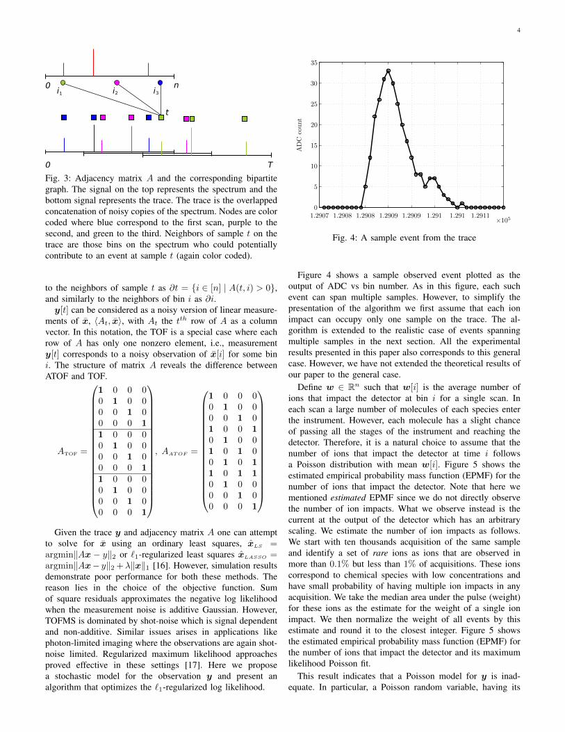
Fig. 4: A sample event from the trace
Figure 4 shows a sample observed event plotted as theoutput of ADC vs bin number. As in this figure, each suchevent can span multiple samples. However, to simplify thepresentation of the algorithm we first assume that each ionimpact can occupy only one sample on the trace. The al-gorithm is extended to the realistic case of events spanningmultiple samples in the next section. All the experimentalresults presented in this paper also corresponds to this generalcase. However, we have not extended the theoretical results ofour paper to the general case.
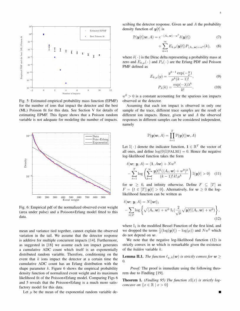
Define w ∈ Rn such that w[i] is the average number ofions that impact the detector at bin i for a single scan. Ineach scan a large number of molecules of each species enterthe instrument. However, each molecule has a slight chanceof passing all the stages of the instrument and reaching thedetector. Therefore, it is a natural choice to assume that thenumber of ions that impact the detector at time i followsa Poisson distribution with mean w[i]. Figure 5 shows theestimated empirical probability mass function (EPMF) for thenumber of ions that impact the detector. Note that here wementioned estimated EPMF since we do not directly observethe number of ion impacts. What we observe instead is thecurrent at the output of the detector which has an arbitraryscaling. We estimate the number of ion impacts as follows.We start with ten thousands acquisition of the same sampleand identify a set of rare ions as ions that are observed inmore than 0.1% but less than 1% of acquisitions. These ionscorrespond to chemical species with low concentrations andhave small probability of having multiple ion impacts in anyacquisition. We take the median area under the pulse (weight)for these ions as the estimate for the weight of a single ionimpact. We then normalize the weight of all events by thisestimate and round it to the closest integer. Figure 5 showsthe estimated empirical probability mass function (EPMF) forthe number of ions that impact the detector and its maximumlikelihood Poisson fit.
This result indicates that a Poisson model for y is inad-equate. In particular, a Poisson random variable, having its
5
Best Poisson fit
Estimated EPMF
Em
pir
ical
PM
Fan
dth
ebes
t(M
L)
Poi
sson
fit
Number of impacts
−2 0 2 4 6 8 10 1210−14
10−12
10−10
10−8
10−6
10−4
10−2
100
102
Fig. 5: Estimated empirical probability mass function (EPMF)for the number of ions that impact the detector and the best(ML) Poisson fit for this data. See Section V for details ofestimating EPMF. This figure shows that a Poisson randomvariable is not adequate for modeling the number of impacts.
ExponentialPois+ErlangData
Den
sity
Event weight100 200 300 400 500 600 700 800 900
10−2
10−1
Fig. 6: Empirical pdf of the normalized observed event weight(area under pulse) and a Poisson+Erlang model fitted to thisdata.
mean and variance tied together, cannot explain the observedvariation in the tail. We assume that the detector responseis additive for multiple concurrent impacts [14]. Furthermore,as suggested in [18] we assume each ion impact generatesa cumulative ADC count which itself is an exponentiallydistributed random variable. Therefore, conditioning on theevent that k ions impact the detector at a certain time thecumulative ADC count has an Erlang distribution with theshape parameter k. Figure 6 shows the empirical probabilitydensity function of normalized event weight and its maximumlikelihood fit of the Poisson+Erlang model. Comparing Figs 6and 5 reveals that the Poisson+Erlang is a much more satis-factory model for this data.
Let µ be the mean of the exponential random variable de-
scribing the detector response. Given w and A the probabilitydensity function of y[t] is
P(y[t]|w, A) = e−〈At,w〉−w0
δ(y[t]) (7)
+
∞∑k=1
Ek,µ(y[t])P〈At,w〉+w0(k), (8)
where δ( · ) is the Dirac delta representing a probability mass atzero and Ek,µ( · ) and Pλ( · ) are the Erlang PDF and PoissonPMF defined as
Ek,µ(y) =yk−1 exp(− y
µ )
µk(k − 1)!, (9)
Pλ(k) =exp(−λ)λk
k!. (10)
w0 > 0 is a constant accounting for the spurious ion impactsobserved at the detector.
Assuming that each ion impact is observed in only onesample of the trace, different trace samples are the result ofdifferent ion impacts. Hence, given w and A the observedresponses in different samples can be considered independent,namely
P(y|w, A) =
T∏t=1
P(y[t]|w, A)
Let I( · ) denote the indicator function, 1 ∈ RT the vector ofall ones, and define log(0)I(FALSE) = 0. Hence the negativelog-likelihood function takes the form
`(w; y, A) = 〈1, Aw〉+Nw0
−T∑t=1
log
( ∞∑k=1
y[t]k(〈At,w〉+ w0)k
(k − 1)! k!µk
)I(y[t] > 0) (11)
for w ≥ 0, and infinity otherwise. Define F ⊆ [T ] asF = {t ∈ [T ]|y[t] > 0}. Alternatively, for w ≥ 0 the log-likelihood function can be written as
`(w; y, A) = N‖w‖1
−∑t∈F
log
{√〈At,w〉+ w0 I1(
2õ
√y[t]〈At,w〉+ w0)
},
(12)
where I1 is the modified Bessel Function of the first kind, andwe dropped the terms 1
2 (log(y[t])− log(µ)) and Nw0 whichdo not depend on w.
We note that the negative log-likelihood function (12) isstrictly convex in w which is remarkable given the existenceof the hidden variable k.
Lemma II.1. The function `y,A(w) is strictly convex for w ≥0.
Proof: The proof is immediate using the following theo-rem due to Findling [19].
Theorem 1. (Findling 95) The function xI(x) is strictly log-concave on {x ∈ R | x > 0}
6
A simple transformation of the negative log-likelihood func-tion (12) is insightful. Let λ = 2Nµ, w = w/µ, then forw ≥ 0,
`(w; y, A) = ˜(w; y,A) + λ‖w‖1, (13)
where
˜(w; y,A) = −∑t∈F
log
√y[t]∑i∈∂t
wi I1
√y[t]∑i∈∂t
wi
.A few remarks are in order. First, note that the scaling ofthe variable w is irrelevant for our purpose and only therelative values are important. Hence, this is a single-parameterrepresentation of the NLL function. This is of great importancefor practical systems where optimal tuning of multiple pa-rameters in different operational scenarios can be complicatedand require additional expertise. Second, the single tuningparameter appears as the multiplicative factor in front of the`1 regularization term. Given our intuition about the effect of`1 regularization [16], [20] the parameter governs the sparsityof the estimate w, i.e., the number of species that appear inthe output. In what follows we free the parameter λ fromour original interpretation of it as the product 2Nµ and referto it as the regularization parameter. Further, we define theregularized negative log-likelihood cost function Cλ(w; y, A)as
Cλ(w; y, A) = ˜(w; y,A) + λ‖w‖1 (14)
III. ALGORITHM
Given the regularized negative log-likelihood cost functionCλ(w; y, A) our algorithm attempts to solve the followingoptimization problem.
minimizew
˜(w; y,A) + λ‖w‖1 , s.t. w ≥ 0, (15)
We use the now standard method of iterative soft thresholdingto solve this convex but non-differentiable optimization prob-lem. For a doubly differentiable function f : D ⊂ Rn → R let∇f and ∇2f be the gradient and Hessian of f respectively.Let γ > 0 be such that ‖∇2 ˜(w; y, A)‖2 < γ−1 for w ≥ 0.It is easy to see that γ exists because of the presence of thechemical noise term w0. We call the parameter γ the step sizeas we use it to scale the steps the algorithm takes in eachiteration. Let w(k) be our estimate of w at step k. Then wecan compute an upper bound for the cost function Cy,A,λ(w)as follows.
Cλ(w; y, A) ≤ ˜(w(k); y, A) +w∗∇˜(w(k); y, A)
+ γ−1‖w −w(k)‖22 + ‖w‖1. (16)
Equation (16) provides an approximation for Cy,A,λ(w) whenw is in a small neighborhood of w(k). Minimizing the right-hand-side of Eq. (16) with respect to w as a surrogate for theactual cost function results in
w(k+1) = ηθ
(w(k) − γ∇˜(w(k); y, A)
). (17)
where ηθ( · ) is the soft thresholding function, ηθ(x) = (|x| −θ)+ with ( · )+ being the positive part and θ ∝ λ−1. Note thatthis is the one-sided soft thresholding function which differs
from the two-sided soft thresholding function by mapping allnegative values to zero. From Eq. (12), ∇˜λ(w; y, A) can becalculated as
∇˜∗λ(w; y, A) = −∑t∈F
(1
2〈At,w〉
+I0
(2√y[t]〈At,w〉
)+ I2
(2√y[t]〈At,w〉
)2√y[t]〈At,w〉I1
(2√y[t]〈At,w〉
) )At. (18)
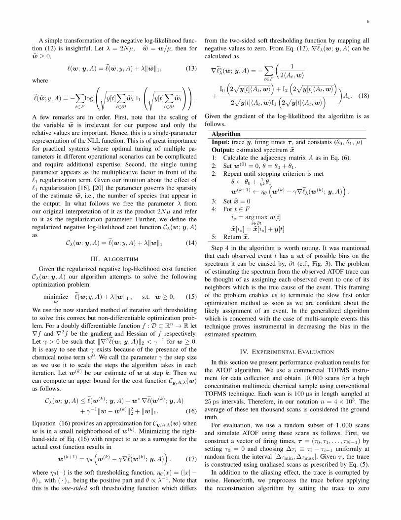
Given the gradient of the log-likelihood the algorithm is asfollows.
AlgorithmInput: trace y, firing times τ , and constants (θ0, θ1, µ)Output: estimated spectrum x1: Calculate the adjacency matrix A as in Eq. (6).2: Set w(0) = 0, θ = θ0 + θ1.2: Repeat until stopping criterion is met
θ ← θ0 + 1k2 θ1
w(k+1) ← ηθ
(w(k) − γ∇˜λ(w(k); y, A)
).
3: Set x = 04: For t ∈ F
i∗ = arg maxi∈∂t
w[i]
x[i∗] = x[i∗] + y[t]5: Return x.
Step 4 in the algorithm is worth noting. It was mentionedthat each observed event t has a set of possible bins on thespectrum it can be caused by, ∂t (c.f., Fig. 3). The problemof estimating the spectrum from the observed ATOF trace canbe thought of as assigning each observed event to one of itsneighbors which is the true cause of the event. This framingof the problem enables us to terminate the slow first orderoptimization method as soon as we are confident about thelikely assignment of an event. In the generalized algorithmwhich is concerned with the case of multi-sample events thistechnique proves instrumental in decreasing the bias in theestimated spectrum.
IV. EXPERIMENTAL EVALUATION
In this section we present performance evaluation results forthe ATOF algorithm. We use a commercial TOFMS instru-ment for data collection and obtain 10, 000 scans for a highconcentration multimode chemical sample using conventionalTOFMS technique. Each scan is 100 µs in length sampled at25 ps intervals. Therefore, in our notation n = 4 × 10⁵. Theaverage of these ten thousand scans is considered the groundtruth.
For evaluation, we use a random subset of 1, 000 scansand simulate ATOF using these scans as follows. First, weconstruct a vector of firing times, τ = (τ0, τ1, . . . , τN−1) bysetting τ0 = 0 and choosing ∆τi ≡ τi − τi−1 uniformly atrandom from the interval [∆τmin,∆τmax]. Given τ , the traceis constructed using unaliased scans as prescribed by Eq. (5).
In addition to the aliasing effect, the trace is corrupted bynoise. Henceforth, we preprocess the trace before applyingthe reconstruction algorithm by setting the trace to zero
7
↔d4d3d2d1 →→←→←→
hw
h0↓↓↓↓↓↓↓↓↓↓↓↓↓↓↓↓
4300 4350 4400 4450 4500 4550 4600 4650 47000
0.02
0.04
0.06
0.08
0.1
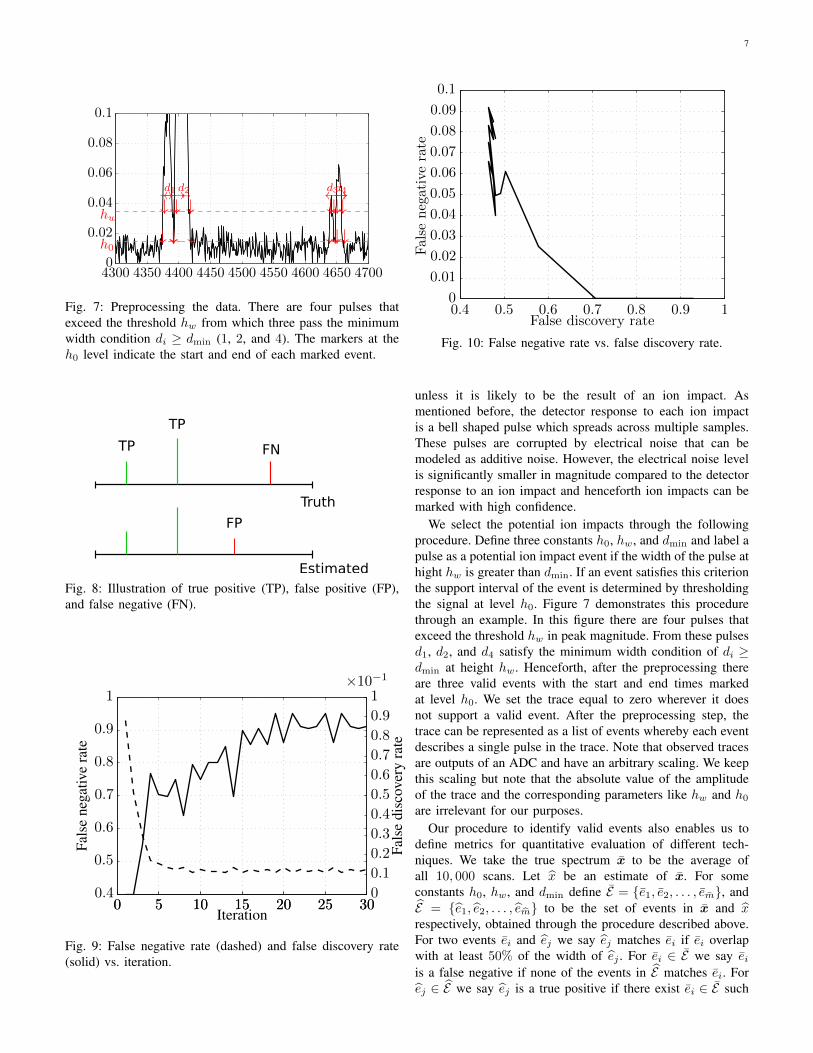
Fig. 7: Preprocessing the data. There are four pulses thatexceed the threshold hw from which three pass the minimumwidth condition di ≥ dmin (1, 2, and 4). The markers at theh0 level indicate the start and end of each marked event.
Fig. 8: Illustration of true positive (TP), false positive (FP),and false negative (FN).
False
discoveryrate
Iteration
False
negativerate
0 5 10 15 20 25 300 5 10 15 20 25 30
×10−1
0
0.1
0.2
0.3
0.4
0.5
0.6
0.7
0.8
0.9
1
0.4
0.5
0.6
0.7
0.8
0.9
1
Fig. 9: False negative rate (dashed) and false discovery rate(solid) vs. iteration.
False discovery rate
Fal
seneg
ativ
era
te
0.4 0.5 0.6 0.7 0.8 0.9 10
0.01
0.02
0.03
0.04
0.05
0.06
0.07
0.08
0.09
0.1
Fig. 10: False negative rate vs. false discovery rate.
unless it is likely to be the result of an ion impact. Asmentioned before, the detector response to each ion impactis a bell shaped pulse which spreads across multiple samples.These pulses are corrupted by electrical noise that can bemodeled as additive noise. However, the electrical noise levelis significantly smaller in magnitude compared to the detectorresponse to an ion impact and henceforth ion impacts can bemarked with high confidence.
We select the potential ion impacts through the followingprocedure. Define three constants h0, hw, and dmin and label apulse as a potential ion impact event if the width of the pulse athight hw is greater than dmin. If an event satisfies this criterionthe support interval of the event is determined by thresholdingthe signal at level h0. Figure 7 demonstrates this procedurethrough an example. In this figure there are four pulses thatexceed the threshold hw in peak magnitude. From these pulsesd1, d2, and d4 satisfy the minimum width condition of di ≥dmin at height hw. Henceforth, after the preprocessing thereare three valid events with the start and end times markedat level h0. We set the trace equal to zero wherever it doesnot support a valid event. After the preprocessing step, thetrace can be represented as a list of events whereby each eventdescribes a single pulse in the trace. Note that observed tracesare outputs of an ADC and have an arbitrary scaling. We keepthis scaling but note that the absolute value of the amplitudeof the trace and the corresponding parameters like hw and h0
are irrelevant for our purposes.Our procedure to identify valid events also enables us to
define metrics for quantitative evaluation of different tech-niques. We take the true spectrum x to be the average ofall 10, 000 scans. Let x be an estimate of x. For someconstants h0, hw, and dmin define E = {e1, e2, . . . , em}, andE = {e1, e2, . . . , em} to be the set of events in x and xrespectively, obtained through the procedure described above.For two events ei and ej we say ej matches ei if ei overlapwith at least 50% of the width of ej . For ei ∈ E we say eiis a false negative if none of the events in E matches ei. Forej ∈ E we say ej is a true positive if there exist ei ∈ E such
8
ATOF-10K
TOF-10KIn
tensi
ty
Mass (Dalton)
500 1000 1500 2000 2500 30000
5
10
15
20
25
30
35
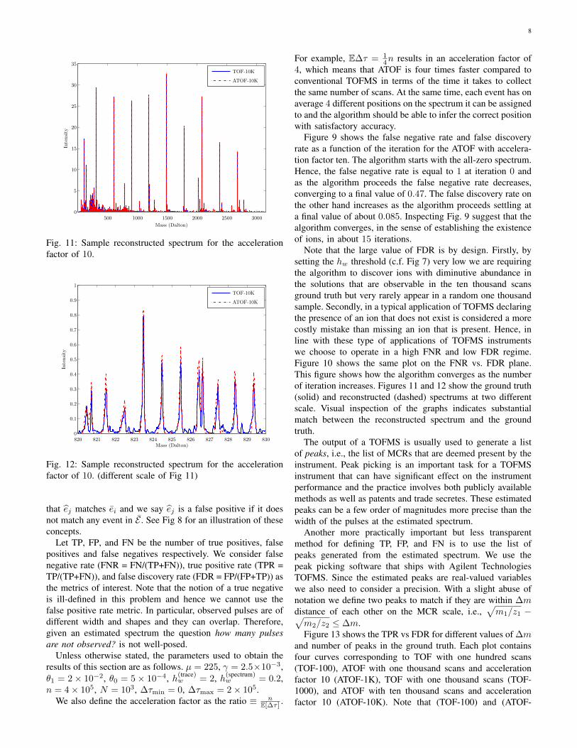
Fig. 11: Sample reconstructed spectrum for the accelerationfactor of 10.
ATOF-10K
TOF-10K
Inte
nsi
ty
Mass (Dalton)820 821 822 823 824 825 826 827 828 829 8300
0.1
0.2
0.3
0.4
0.5
0.6
0.7
0.8
0.9
1
Fig. 12: Sample reconstructed spectrum for the accelerationfactor of 10. (different scale of Fig 11)
that ej matches ei and we say ej is a false positive if it doesnot match any event in E . See Fig 8 for an illustration of theseconcepts.
Let TP, FP, and FN be the number of true positives, falsepositives and false negatives respectively. We consider falsenegative rate (FNR = FN/(TP+FN)), true positive rate (TPR =TP/(TP+FN)), and false discovery rate (FDR = FP/(FP+TP)) asthe metrics of interest. Note that the notion of a true negativeis ill-defined in this problem and hence we cannot use thefalse positive rate metric. In particular, observed pulses are ofdifferent width and shapes and they can overlap. Therefore,given an estimated spectrum the question how many pulsesare not observed? is not well-posed.
Unless otherwise stated, the parameters used to obtain theresults of this section are as follows. µ = 225, γ = 2.5×10⁻³,θ1 = 2× 10⁻², θ0 = 5× 10⁻⁴, h(trace)
w = 2, h(spectrum)w = 0.2,
n = 4× 10⁵, N = 103, ∆τmin = 0, ∆τmax = 2× 10⁵.We also define the acceleration factor as the ratio ≡ n
E[∆τ ] .
For example, E∆τ = 14n results in an acceleration factor of
4, which means that ATOF is four times faster compared toconventional TOFMS in terms of the time it takes to collectthe same number of scans. At the same time, each event has onaverage 4 different positions on the spectrum it can be assignedto and the algorithm should be able to infer the correct positionwith satisfactory accuracy.
Figure 9 shows the false negative rate and false discoveryrate as a function of the iteration for the ATOF with accelera-tion factor ten. The algorithm starts with the all-zero spectrum.Hence, the false negative rate is equal to 1 at iteration 0 andas the algorithm proceeds the false negative rate decreases,converging to a final value of 0.47. The false discovery rate onthe other hand increases as the algorithm proceeds settling ata final value of about 0.085. Inspecting Fig. 9 suggest that thealgorithm converges, in the sense of establishing the existenceof ions, in about 15 iterations.
Note that the large value of FDR is by design. Firstly, bysetting the hw threshold (c.f. Fig 7) very low we are requiringthe algorithm to discover ions with diminutive abundance inthe solutions that are observable in the ten thousand scansground truth but very rarely appear in a random one thousandsample. Secondly, in a typical application of TOFMS declaringthe presence of an ion that does not exist is considered a morecostly mistake than missing an ion that is present. Hence, inline with these type of applications of TOFMS instrumentswe choose to operate in a high FNR and low FDR regime.Figure 10 shows the same plot on the FNR vs. FDR plane.This figure shows how the algorithm converges as the numberof iteration increases. Figures 11 and 12 show the ground truth(solid) and reconstructed (dashed) spectrums at two differentscale. Visual inspection of the graphs indicates substantialmatch between the reconstructed spectrum and the groundtruth.
The output of a TOFMS is usually used to generate a listof peaks, i.e., the list of MCRs that are deemed present by theinstrument. Peak picking is an important task for a TOFMSinstrument that can have significant effect on the instrumentperformance and the practice involves both publicly availablemethods as well as patents and trade secretes. These estimatedpeaks can be a few order of magnitudes more precise than thewidth of the pulses at the estimated spectrum.
Another more practically important but less transparentmethod for defining TP, FP, and FN is to use the list ofpeaks generated from the estimated spectrum. We use thepeak picking software that ships with Agilent TechnologiesTOFMS. Since the estimated peaks are real-valued variableswe also need to consider a precision. With a slight abuse ofnotation we define two peaks to match if they are within ∆mdistance of each other on the MCR scale, i.e.,
√m1/z1 −√
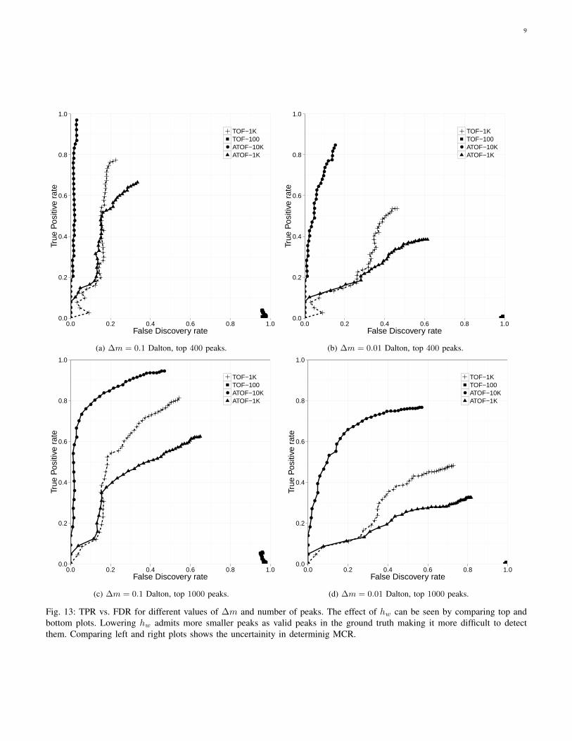
m2/z2 ≤ ∆m.Figure 13 shows the TPR vs FDR for different values of ∆m
and number of peaks in the ground truth. Each plot containsfour curves corresponding to TOF with one hundred scans(TOF-100), ATOF with one thousand scans and accelerationfactor 10 (ATOF-1K), TOF with one thousand scans (TOF-1000), and ATOF with ten thousand scans and accelerationfactor 10 (ATOF-10K). Note that (TOF-100) and (ATOF-
9
0.0
0.2
0.4
0.6
0.8
1.0
●
●
●
●
●
●
●
●●
●
●
●●
●
●
●
●
●
●●
●
●
●
●
●
●
●
●
●
●
●●
●
●●●
●
●
●●
0.0 0.2 0.4 0.6 0.8 1.0False Discovery rate
True
Pos
itive
rat
e
●
TOF−1KTOF−100ATOF−10KATOF−1K
(a) ∆m = 0.1 Dalton, top 400 peaks.
0.0
0.2
0.4
0.6
0.8
1.0
●
●
●
●
●
●
●
●●
●
●
●●
●
●●
●
●●●
●
●●
●●●●●
●●●●●●● ●
●●●●
0.0 0.2 0.4 0.6 0.8 1.0False Discovery rate
True
Pos
itive
rat
e
●
TOF−1KTOF−100ATOF−10KATOF−1K
(b) ∆m = 0.01 Dalton, top 400 peaks.
0.0
0.2
0.4
0.6
0.8
1.0
●
●
●
●
●
●
●
●
●
●
●
●
●
●
●
●
●
●
●●
●●
● ●● ● ●
● ●●●●●●●●●●●●
0.0 0.2 0.4 0.6 0.8 1.0False Discovery rate
True
Pos
itive
rat
e
●
TOF−1KTOF−100ATOF−10KATOF−1K
(c) ∆m = 0.1 Dalton, top 1000 peaks.
0.0
0.2
0.4
0.6
0.8
1.0
●
●
●
●
●
●
●
●
●
●
●
●
●
●●
●
●●
●●
●●
● ● ● ● ●● ● ●●●●●●●●●●●
0.0 0.2 0.4 0.6 0.8 1.0False Discovery rate
True
Pos
itive
rat
e
●
TOF−1KTOF−100ATOF−10KATOF−1K
(d) ∆m = 0.01 Dalton, top 1000 peaks.
Fig. 13: TPR vs. FDR for different values of ∆m and number of peaks. The effect of hw can be seen by comparing top andbottom plots. Lowering hw admits more smaller peaks as valid peaks in the ground truth making it more difficult to detectthem. Comparing left and right plots shows the uncertainity in determinig MCR.
10
0.0
0.2
0.4
0.6
0.8
1.0
1e−04 1e−02width (FWHM) to intensity ratio
EC
DF
TOF−10KTOF−1KATOF−10KATOF−1K
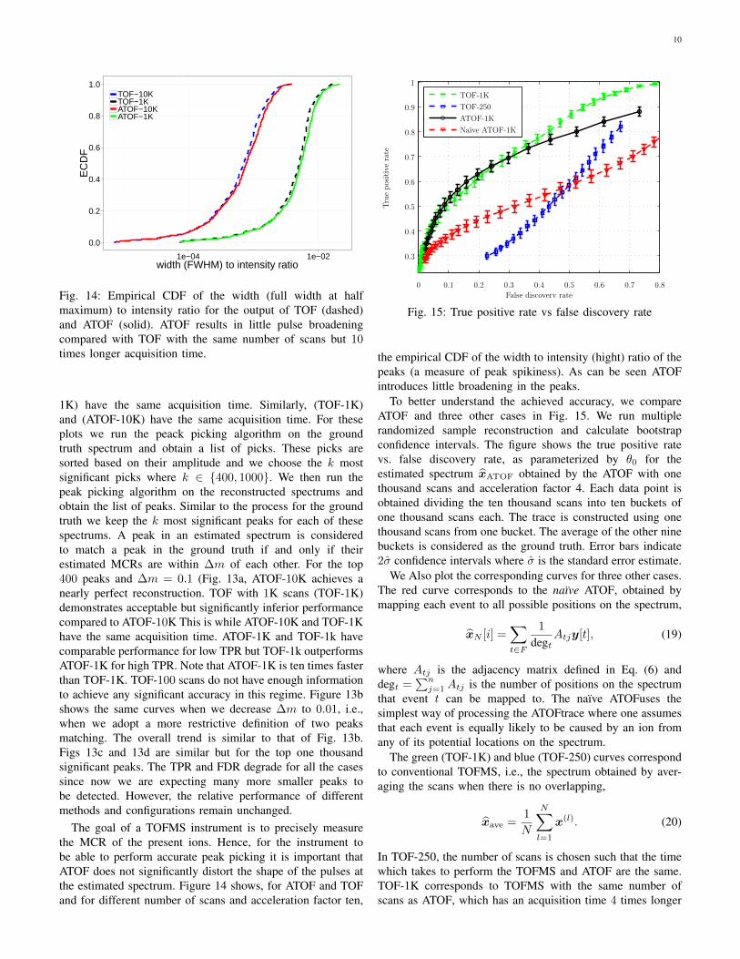
Fig. 14: Empirical CDF of the width (full width at halfmaximum) to intensity ratio for the output of TOF (dashed)and ATOF (solid). ATOF results in little pulse broadeningcompared with TOF with the same number of scans but 10times longer acquisition time.
1K) have the same acquisition time. Similarly, (TOF-1K)and (ATOF-10K) have the same acquisition time. For theseplots we run the peack picking algorithm on the groundtruth spectrum and obtain a list of picks. These picks aresorted based on their amplitude and we choose the k mostsignificant picks where k ∈ {400, 1000}. We then run thepeak picking algorithm on the reconstructed spectrums andobtain the list of peaks. Similar to the process for the groundtruth we keep the k most significant peaks for each of thesespectrums. A peak in an estimated spectrum is consideredto match a peak in the ground truth if and only if theirestimated MCRs are within ∆m of each other. For the top400 peaks and ∆m = 0.1 (Fig. 13a, ATOF-10K achieves anearly perfect reconstruction. TOF with 1K scans (TOF-1K)demonstrates acceptable but significantly inferior performancecompared to ATOF-10K This is while ATOF-10K and TOF-1Khave the same acquisition time. ATOF-1K and TOF-1k havecomparable performance for low TPR but TOF-1k outperformsATOF-1K for high TPR. Note that ATOF-1K is ten times fasterthan TOF-1K. TOF-100 scans do not have enough informationto achieve any significant accuracy in this regime. Figure 13bshows the same curves when we decrease ∆m to 0.01, i.e.,when we adopt a more restrictive definition of two peaksmatching. The overall trend is similar to that of Fig. 13b.Figs 13c and 13d are similar but for the top one thousandsignificant peaks. The TPR and FDR degrade for all the casessince now we are expecting many more smaller peaks tobe detected. However, the relative performance of differentmethods and configurations remain unchanged.
The goal of a TOFMS instrument is to precisely measurethe MCR of the present ions. Hence, for the instrument tobe able to perform accurate peak picking it is important thatATOF does not significantly distort the shape of the pulses atthe estimated spectrum. Figure 14 shows, for ATOF and TOFand for different number of scans and acceleration factor ten,
Naıve ATOF-1K
ATOF-1K
TOF-250
TOF-1K
Truepositiverate
False discovery rate
0 0.1 0.2 0.3 0.4 0.5 0.6 0.7 0.8
0.3
0.4
0.5
0.6
0.7
0.8
0.9
1
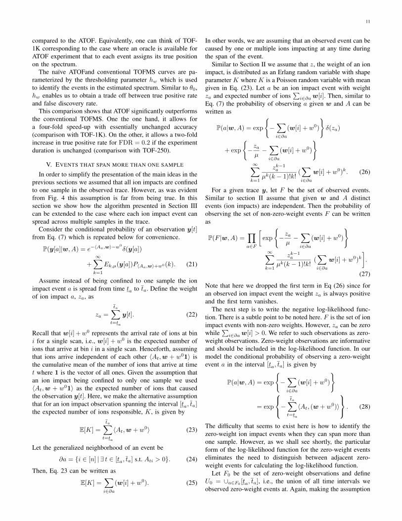
Fig. 15: True positive rate vs false discovery rate
the empirical CDF of the width to intensity (hight) ratio of thepeaks (a measure of peak spikiness). As can be seen ATOFintroduces little broadening in the peaks.
To better understand the achieved accuracy, we compareATOF and three other cases in Fig. 15. We run multiplerandomized sample reconstruction and calculate bootstrapconfidence intervals. The figure shows the true positive ratevs. false discovery rate, as parameterized by θ0 for theestimated spectrum xATOF obtained by the ATOF with onethousand scans and acceleration factor 4. Each data point isobtained dividing the ten thousand scans into ten buckets ofone thousand scans each. The trace is constructed using onethousand scans from one bucket. The average of the other ninebuckets is considered as the ground truth. Error bars indicate2σ confidence intervals where σ is the standard error estimate.
We Also plot the corresponding curves for three other cases.The red curve corresponds to the naıve ATOF, obtained bymapping each event to all possible positions on the spectrum,
xN [i] =∑t∈F
1
degtAtjy[t], (19)
where Atj is the adjacency matrix defined in Eq. (6) anddegt =
∑nj=1Atj is the number of positions on the spectrum
that event t can be mapped to. The naıve ATOFuses thesimplest way of processing the ATOFtrace where one assumesthat each event is equally likely to be caused by an ion fromany of its potential locations on the spectrum.
The green (TOF-1K) and blue (TOF-250) curves correspondto conventional TOFMS, i.e., the spectrum obtained by aver-aging the scans when there is no overlapping,
xave =1
N
N∑l=1
x(l). (20)
In TOF-250, the number of scans is chosen such that the timewhich takes to perform the TOFMS and ATOF are the same.TOF-1K corresponds to TOFMS with the same number ofscans as ATOF, which has an acquisition time 4 times longer
11
compared to the ATOF. Equivalently, one can think of TOF-1K corresponding to the case where an oracle is available forATOF experiment that to each event assigns its true positionon the spectrum.
The naıve ATOFand conventional TOFMS curves are pa-rameterized by the thresholding parameter hw which is usedto identify the events in the estimated spectrum. Similar to θ0,hw enables us to obtain a trade off between true positive rateand false discovery rate.
This comparison shows that ATOF significantly outperformsthe conventional TOFMS. One the one hand, it allows fora four-fold speed-up with essentially unchanged accuracy(comparison with TOF-1K). On the other, it allows a two-foldincrease in true positive rate for FDR = 0.2 if the experimentduration is unchanged (comparison with TOF-250).
V. EVENTS THAT SPAN MORE THAN ONE SAMPLE
In order to simplify the presentation of the main ideas in theprevious sections we assumed that all ion impacts are confinedto one sample in the observed trace. However, as was evidentfrom Fig. 4 this assumption is far from being true. In thissection we show how the algorithm presented in Section IIIcan be extended to the case where each ion impact event canspread across multiple samples in the trace.
Consider the conditional probability of an observation y[t]from Eq. (7) which is repeated below for convenience.
P(y[a]|w, A) = e−〈Aa,w〉−w0
δ(y[a])
+
∞∑k=1
Ek,µ(y[a])P〈Aa,w〉+w0(k). (21)
Assume instead of being confined to one sample the ionimpact event a is spread from time ta to ta. Define the weightof ion impact a, za, as
za =
ta∑t=ta
y[t]. (22)
Recall that w[i] +w0 represents the arrival rate of ions at bini for a single scan, i.e., w[i] + w0 is the expected number ofions that arrive at bin i in a single scan. Henceforth, assumingthat ions arrive independent of each other 〈At,w + w01〉 isthe cumulative mean of the number of ions that arrive at timet where 1 is the vector of all ones. Given the assumption thatan ion impact being confined to only one sample we used〈At,w + w01〉 as the expected number of ions that causedthe observation y[t]. Here, we make the alternative assumptionthat for an ion impact observation spanning the interval [ta, ta]the expected number of ions responsible, K, is given by
E[K] =
ta∑t=ta
〈At,w + w0〉 (23)
Let the generalized neighborhood of an event be
∂a = {i ∈ [n] | ∃ t ∈ [ta, ta] s.t. Ati > 0}. (24)
Then, Eq. 23 can be written as
E[K] =∑i∈∂a
(w[i] + w0). (25)
In other words, we are assuming that an observed event can becaused by one or multiple ions impacting at any time duringthe span of the event.
Similar to Section II we assume that z, the weight of an ionimpact, is distributed as an Erlang random variable with shapeparameter K where K is a Poisson random variable with meangiven in Eq. (23). Let a be an ion impact event with weightza and expected number of ions
∑i∈∂aw[i]. Then, similar to
Eq. (7) the probability of observing a given w and A can bewritten as
P(a|w, A) = exp
{−∑i∈∂a
(w[i] + w0)
}δ(za)
+ exp
{−zaµ−∑i∈∂a
(w[i] + w0)
}∞∑k=1
zk−1a
µk(k − 1)!k!(∑i∈∂a
w[i] + w0)k. (26)
For a given trace y, let F be the set of observed events.Similar to section II assume that given w and A distinctevents (ion impacts) are independent. Then the probability ofobserving the set of non-zero-weight events F can be writtenas
P(F |w, A) =∏a∈F
[exp
{−zaµ−∑i∈∂a
(w[i] + w0)
}∞∑k=1
zk−1a
µk(k − 1)!k!(∑i∈∂a
w[i] + w0)k].
(27)
Note that here we dropped the first term in Eq (26) since foran observed ion impact event the weight za is always positiveand the first term vanishes.
The next step is to write the negative log-likelihood func-tion. There is a subtle point to be noted here. F is the set of ionimpact events with non-zero weights. However, za can be zerowhile
∑i∈∂aw[i] > 0. We refer to such observations as zero-
weight observations. Zero-weight observations are informativeand should be included in the log-likelihood function. In ourmodel the conditional probability of observing a zero-weightevent a in the interval [ta, ta] is given by
P(a|w, A) = exp
{−∑i∈∂a
(w[i] + w0)
}
= exp
−ta∑t=ta
〈At, (w + w0)〉
. (28)
The difficulty that seems to exist here is how to identify thezero-weight ion impact events when they can span more thanone sample. However, as we shall see shortly, the particularform of the log-likelihood function for the zero-weight eventseliminates the need to distinguish between adjacent zero-weight events for calculating the log-likelihood function.
Let F0 be the set of zero-weight observations and defineU0 = ∪a∈F0
[ta, ta], i.e., the union of all time intervals weobserved zero-weight events at. Again, making the assumption
12
that distinct zero-weight ion impacts are independent eventsgiven w and A we can write the joint probability of observingF0 as
P(F0|w, A) =∏a∈F0
exp
{−∑i∈∂a
w[i]
}
=∏a∈F0
exp
−ta∑t=ta
〈At,w〉
= exp(−
∑t∈U0
〈At,w〉). (29)
Note that P(F0|w, A) does not depend on the number of zero-weight events or the beginning or end time of a particularevent. We need only to identify all the samples that are partof a zero-weight event, i.e., not part of any observed ion impactevent.
Putting Equations (27) and (29) together and assuming thatall the events are independent we have the probability ofobserving a trace y as
P(y|w, A) = P(F |w, A)P(F0|w, A)
= exp
{−∑a∈F0
∑i∈∂a
(w[i] + w0)
}
exp
{−∑a∈F
∑i∈∂a
(w[i] + w0)− zaµ
}∏a∈F
[ ∞∑k=1
zk−1a
µk(k − 1)!k!
(∑i∈∂a
(w[i] + w0)
)k]
= exp
{−N‖w‖1 −
∑a∈F
zaµ
}∏a∈F
∞∑k=1
zk−1a
µk(k − 1)!k!
(∑i∈∂a
(w[i] + w0)
)k ,(30)
where the last equality is obtained since each sample onthe trace is presented in either F or F0. The negative log-likelihood function then can be written as
`(w|y, A) = −N‖w‖1
−∑a∈F
log
∞∑k=1
zkaµk(k − 1)!k!
(∑i∈∂a
(w[i] + w0)
)k(31)
After some algebra, and keeping only the terms that dependon w,
`(w|y, A) =−N‖w‖1
−∑a∈F
[1
2log
(∑i∈∂a
(w[i] + w0)
µ
)
+ log I1
(2
√za∑i∈∂a
(w[i] + w0)
µ
)], (32)
Using the same change of variable as before, namely w =1µw, λ = Nµ and ˜(w|y, A) = `(w|y, A)−N‖w‖1 we have`(w|y, A) = ˜(w|y, A) + λ‖w‖1 where
˜(w|y, A) =−∑a∈F
[1
2log
(∑i∈∂a
(w[i] + w0)
)
+ log I1
2
√za∑i∈∂a
(w[i] + w0)
], (33)
And the gradient of the function ˜(w|y, A) is
∇˜(w|y, A) = −∑a∈F
ta∑t=ta
At
[1
2∑i∈∂a(w[i] + w0)
+
I0(2
√za∑i∈∂a
(w[i] + w0)) + I2(2
√za∑i∈∂a
(w[i] + w0))
2
√za∑i∈∂a
(w[i] + w0)I1(2
√za∑i∈∂a
(w[i] + w0))
−1 ](34)
Having the gradient of the log-likelihood function the algo-rithm is similar to the algorithm of section III with the gradientof the log-likelihood calculated using Eq. (34). However, weneed some additional notations to represent the generalizedalgorithm. Let deg(a) be the number of neighbors of event a,i.e., deg(a) =
∑ni=1Ata,i
1. For j ∈ [deg(a)] let ija be theindex of the jth non-zero element of Ata . Similarly, let i
ja be
the index of the jth non-zero element of Ata . Then, [ija, ija] is
the true position of event a on the spectrum if its jth neighborcorresponds to the true scan that caused event a.
The peak picking algorithms are usually sensitive to theshape of the pulses. Furthermore, the time of arrival of theions are noisier than the observation error of the instrument.Observing many scans enables the instrument to measure theMCR of the ions with precision significantly better than thearrival noise level. To overcome the issue of a possible bias inthe estimated MCR in our model, we employ one last trick.The algorithm constructs an estimate of the spectrum x byassigning each observed event to its most likely neighbor (c.f.Fig. 3). In other words, let
j∗ = arg maxj∈[deg(a)]
ija∑
i=ija
w[i]. (35)
Then, given w we reconstruct the estimated spectrum as
x[ij∗
a + ∆] = x[ij∗
a + ∆] + y[t+ ∆]. (36)
Using this notation the algorithm as as follows.
1This definition is slightly inaccurate since an event can potentially fall onthe boundary of an scan resulting in
∑ni=1 Ata,i
6=∑n
i=1 Ata,ibut this is
rare and the discrepancy is negligible.
13
AlgorithmInput: trace y, firing times τ , and constants (θ0, θ1, λ, γ)Output: estimated spectrum x1: Calculate the adjacency matrix A as in Eq. (6).2: Set w(0) = 0, θ = θ0 + θ1.2: Repeat until stopping criterion is met:
θ ← θ0 + 1k2 θ1
w(k+1) ← ηθ
(w(k) − γ∇˜(w(k); y, A)
).
3: Set x = 04: For a ∈ F :
j∗ = arg maxj∈[deg(a)]
∑ija
i=ijaw[i]
For ∆ = 0, . . . , (ta − ta):x[ij
∗
a + ∆] = x[ij∗
a + ∆] + y[t+ ∆]5: Return x.
REFERENCES
[1] Franz Hillenkamp, Michael Karas, Ronald C. Beavis, and Brian T.Chait, “Matrix-assisted laser desorption/ionization mass spectrometry ofbiopolymers,” Analytical Chemistry, vol. 63, no. 24, pp. 1193A–1203A,1991, PMID: 1789447.
[2] J.B. Fenn, M. Mann, C.K. Meng, S.F. Wong, C.M. Whitehouse, et al.,“Electrospray ionization for mass spectrometry of large biomolecules.,”Science (New York, NY), vol. 246, no. 4926, pp. 64, 1989.
[3] Franz Hillenkamp, Michael Karas, Ronald C. Beavis, and Brian T.Chait, “Matrix-assisted laser desorption/ionization mass spectrometry ofbiopolymers,” Analytical Chemistry, vol. 63, no. 24, pp. 1193A–1203A,1991, PMID: 1789447.
[4] J. Ragoussis, G.P. Elvidge, K. Kaur, and S. Colella, “Matrix-assistedlaser desorption/ionisation, time-of-flight mass spectrometry in genomicsresearch,” PLoS genetics, vol. 2, no. 7, pp. e100, 2006.
[5] W.G. Cross, “Two-directional focusing of charged particles with asector-shaped, uniform magnetic field,” Review of Scientific Instruments,vol. 22, no. 10, pp. 717–722, 1951.
[6] J.C. Schwartz, M.W. Senko, and J.E.P. Syka, “A two-dimensionalquadrupole ion trap mass spectrometer,” Journal of the American Societyfor Mass Spectrometry, vol. 13, no. 6, pp. 659–669, 2002.
[7] W.E. Stephens, “A pulsed mass spectrometer with time dispersion,”Phys. Rev, vol. 69, no. 691, pp. 46, 1946.
[8] M.T. Roberts, J.P. Dufour, and A.C. Lewis, “Application of comprehen-sive multidimensional gas chromatography combined with time-of-flightmass spectrometry (GC× GC-TOFMS) for high resolution analysis ofhop essential oil,” Journal of separation science, vol. 27, no. 5-6, pp.473–478, 2004.
[9] J.B. Fenn, “Electrospray wings for molecular elephants (nobel lecture),”Angewandte Chemie International Edition, vol. 42, no. 33, pp. 3871–3894, 2003.
[10] A. Shevchenko, I. Chernushevich, W. Ens, K.G. Standing, B. Thomson,M. Wilm, and M. Mann, “Rapid’de novo’peptide sequencing by a com-bination of nanoelectrospray, isotopic labeling and a quadrupole/time-of-flight mass spectrometer,” Rapid Communications in Mass Spectrometry,vol. 11, no. 9, pp. 1015–1024, 1997.
[11] John S Janiszewski, Theodore E Liston, and Mark J Cole, “Perspectiveson bioanalytical mass spectrometry and automation in drug discovery,”Current drug metabolism, vol. 9, no. 9, pp. 986–994, 2008.
[12] O. Trapp, J.R. Kimmel, O.K. Yoon, I.A. Zuleta, F.M. Fernandez, andR.N. Zare, “Continuous two-channel time-of-flight mass spectrometricdetection of electrosprayed ions,” Angewandte Chemie InternationalEdition, vol. 43, no. 47, pp. 6541–6544, 2004.
[13] F.J. Knorr, M. Ajami, and D.A. Chatfield, “Fourier transform time-of-flight mass spectrometry,” Analytical Chemistry, vol. 58, no. 4, pp.690–694, 1986.
[14] A. Brock, N. Rodriguez, and R.N. Zare, “Hadamard transform time-of-flight mass spectrometry,” Analytical Chemistry, vol. 70, no. 18, pp.3735–3741, 1998.
[15] G.S. Moore, M. Manlove, and A. Hidalgo, “Statistical Inference Al-gorithm for DitheredMulti-Pulsing Time-of-Flight Mass Spectrometry,”Submitted, 2012.
[16] Robert Tibshirani, “Regression shrinkage and selection via the lasso,”Journal of the Royal Statistical Society. Series B (Methodological), pp.267–288, 1996.
[17] Z. Harmany, R. Marcia, and R. Willett, “This is SPIRAL-TAP: SparsePoisson Intensity Reconstruction ALgorithms– Theory and Practice,”Image Processing, IEEE Transactions on, , no. 99, pp. 1–1, 2010.
[18] J.L. Wiza, “Microchannel plate detectors,” Nucl. Instrum. Methods, vol.162, no. 1-3, pp. 587–601, 1979.
[19] A. Findling, “A family of logarithmically concave functions defined byan integral over the modified bessel function of order 1,” Journal ofmathematical analysis and applications, vol. 194, no. 2, pp. 368–376,1995.
[20] Peng Zhao and Bin Yu, “On model selection consistency of lasso,” TheJournal of Machine Learning Research, vol. 7, pp. 2541–2563, 2006.
14
PLACEPHOTOHERE
Morteza Ibrahimi Morteza Ibrahimi received hisPhD in Electrical Engineering from Stanford Uni-versity in 2013, working with professor AndreaMontanari. His research interests are in high dimen-sional statistical signal processing, learning graphi-cal models, optimization through message passingalgorithms, and statistical inference with high di-mensional data, specially through fast iterative algo-rithms. He received his BS from Sharif Universityof Technology in 2006, and MSc from University ofToronto in 2007.
PLACEPHOTOHERE
Andrea Montanari Andrea Montanari received aLaurea degree in Physics in 1997, and a Ph. D.in Theoretical Physics in 2001 (both from ScuolaNormale Superiore in Pisa, Italy). He has been post-doctoral fellow at Laboratoire de Physique Thoriquede l’Ecole Normale Suprieure (LPTENS), Paris,France, and the Mathematical Sciences ResearchInstitute, Berkeley, USA. Since 2002 he is Chargde Recherche (with Centre National de la RechercheScientifique, CNRS) at LPTENS. In September 2006he joined Stanford University as a faculty, and since
2010 he is Associate Professor in the Departments of Electrical Engineeringand Statistics. He was co-awarded the ACM SIGMETRICS best paper awardin 2008. He received the CNRS bronze medal for theoretical physics in 2006and the National Science Foundation CAREER award in 2008.
PLACEPHOTOHERE
George Moore Goerge S. Moore is a researchfellow at Agilent technology. He received his PhD in1980 from Purdue University and his Bsc/Msc fromMississippi State University in 1974 all in ElectricalEngineering. He has over 40 years of experience inthe industry.