abdel1
TRANSCRIPT

1
Abdel H. El-ShaarawiNational Water Research Institute and
Department of Mathematics and Statistics, McMaster University
Data-driven and Physically-based Models for Characterization of Processes in Hydrology,
Hydraulics, Oceanography and Climate Change
January 6-28, 2008IMS, Singapore
Modeling Extreme Events Data

2
Outline
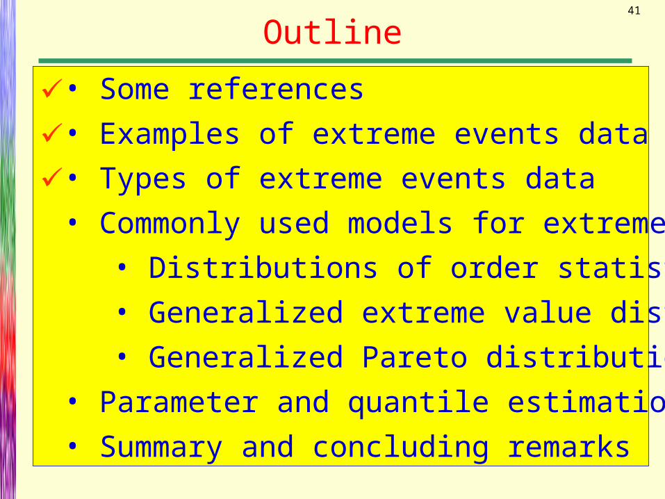
• Some references
• Examples of extreme events data
• Types of extreme events data
• Commonly used models for extremes:
• Distributions of order statistics
• Generalized extreme value distributions
• Generalized Pareto distributions
• Parameter and quantile estimation of extremes
• Summary and concluding remarks

3
References
Beirlant Jan, Yuri Goegebeur, Johan Segers and Jozef Teugels (2004), Statistics of Extremes: Theory and Applications, NewYork: John Wiley & Sons.
Castillo, E. and Hadi, A. S. (1994), Parameter and Quantile Estimation for the Generalized Extreme-Value Distribution, Environmetrics, 5, 417–432.
Castillo, E. and Hadi, A. S. (1995), A Method for Estimating Parameters and Quantiles of Continuous Distributions of Random Variables, Computational Statistics and Data Analysis, 20, 421–439.

4
References
• Castillo, E., Hadi, A. S., Balakrishnan, N., and Sarabia, J. M. (2006), Extreme Value and Related Models in Engineering and Science Applications, New York: John Wiley & Sons.
Coles, S. (2001). An Introduction to Statistical Modeling of Extreme Values. Springer-Verlag, London, England.
El-Shaarawi, A. H., and Hadi, A. S.,Modified Likelihood Function for Parameter and Quantile Estimation, Work in progress.
Nadarajah, S. and El-Shaarawi, A. H. (2006). On the Ratios for Extreme Value Distributions with Applications to Rainfall Modeling. Environmetrics
Kotz, S. and Nadarajah, S. (2000). Extreme Value Distributions: Theory and Applications. London: Imperial College Press.

5
Software: S-plus & R
• Stuart Coles S-plus package available at URL:http://www.math.lancs.ac.uk./~coless
• extRemes R package available at http://www.isse.ucar.edu/extremevalues

6
Examples of Extreme Events Data
In many statistical applications, the interest is centered on estimating some population characteristics based on random samples taken from a population under study.
For example, we wish to estimate:• the average rainfall, • the average temperature, • the median income, • … etc.

7
Examples of Extreme Events Data
In other areas of applications, we are not interested in estimating the average but rather in estimating the maximum or the minimum.
1. Ocean Engineering: In the design of offshore platforms, breakwaters, dikes and other harbor works, engineers rely upon the knowledge of the probability distribution of the maximum, not the average wave height.
Some Examples:

8
Examples of Extreme Events Data
2. Structural Engineering: Modern building codes and standards require: •Estimation of extreme wind speeds
and their recurrence intervals during the lifetime of the building.
•Knowledge of the largest loads acting on the structure during its lifetime.
•Seismic incidence: the maximum earthquake intensity during the lifetime of the building.

9
Examples of Extreme Events Data3. Designing Dams: Engineers would
not be interested in the probability distribution of the average flood, but in the maximum floods.
4. Agriculture: Farmers would be interested in both the minimum and maximum rain fall (drought versus flooding).
5. Insurance companies would be interested in the maximum insurance claims.
10
Examples of Extreme Events Data6. Pollution Control: The pollution of air
and water has become a common problem in many countries due to large concentrations of people, traffic, and industries (producing smoke, human, chemical, nuclear wastes, etc.). Government regulations, require pollution indices to remain below a given critical level. Thus, the regulations are satisfied if, and only if, the largest pollution concentration during the period of interest is less than the critical level.

11
Nile meter

12
U.S. Bureau of the census, Watson and Pauly (2002)
Living resources: food security

13
Niagara River Fraser River

14
Upstream-Downstream Water Quality MonitoringHuman and Ecosystem Health: Regulations and Control
S0 S1 S2 . . . Sk-1 Sk
Niagara River
Overview of U-D M: Purpose, Design and Examples Univariate Series and Ratio (Trend & Seasonality) Bivariate Series
Fraser River Several Stations
Date Julian DayDaily Flow
(m3/s)
Nitrogen Total
Dissolved (mg/L)
Phosphorus Total (mg/L)
Daily Flow (m3/s)
Nitrogen Total
Dissolved (mg/L)
Phosphorus Total (mg/L)
Daily Flow (m3/s)
Nitrogen Total
Dissolved (mg/L)
Phosphorus Total (mg/L)
Daily Flow (m3/s)
Nitrogen Total
Dissolved (mg/L)
Phosphorus Total (mg/L)
3/1/1912 61 #N/A #N/A #N/A #N/A #N/A #N/A #N/A #N/A #N/A 538 #N/A #N/A3/2/1912 62 #N/A #N/A #N/A #N/A #N/A #N/A #N/A #N/A #N/A 538 #N/A #N/A3/3/1912 63 #N/A #N/A #N/A #N/A #N/A #N/A #N/A #N/A #N/A 538 #N/A #N/A
12/27/2003 361 8.4 #N/A #N/A 113 #N/A #N/A 430 #N/A #N/A 740 #N/A #N/A12/28/2003 362 8.07 #N/A #N/A 108 #N/A #N/A 429 #N/A #N/A 730 #N/A #N/A12/29/2003 363 7.79 #N/A #N/A 104 #N/A #N/A 423 #N/A #N/A 720 #N/A #N/A12/30/2003 364 7.61 #N/A #N/A 101 #N/A #N/A 417 #N/A #N/A 720 #N/A #N/A12/31/2003 365 7.49 #N/A #N/A 96.7 #N/A #N/A 416 #N/A #N/A 720 #N/A #N/A
1700 km2 18000 km2 114000 km2 217000 km2Fraser River at Red Pass Fraser River at Hansard Fraser River at Marguerite Fraser River at Hope
15
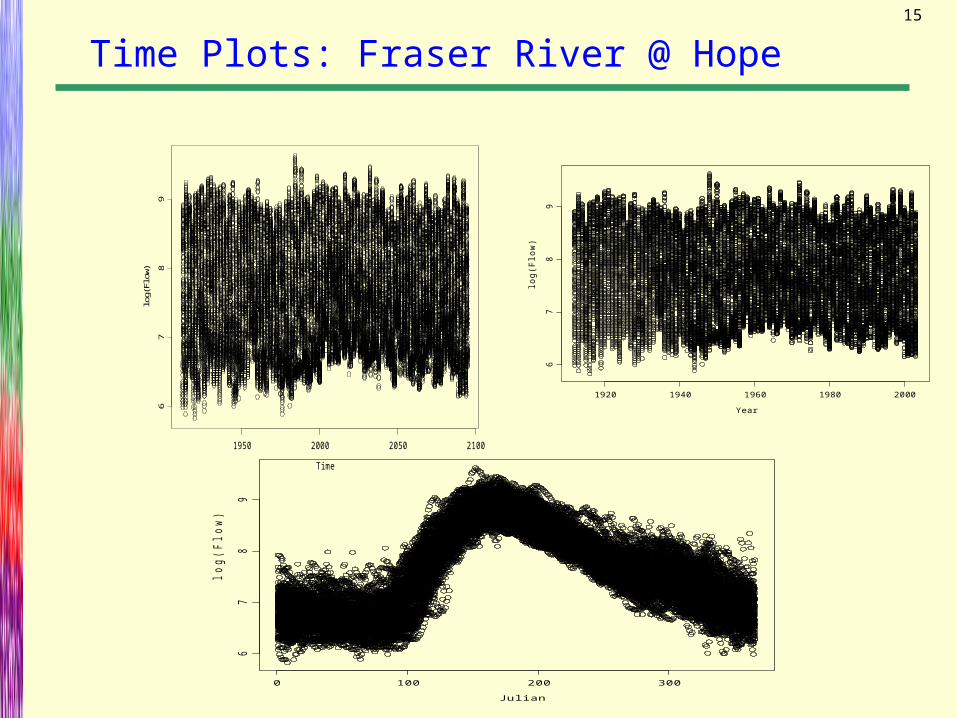
Time Plots: Fraser River @ Hope
Time
log(
Flow
)
1950 2000 2050 2100
67
89
Year
log
(Flo
w)
1920 1940 1960 1980 2000
67
89
Julian
log
(Flo
w)
0 100 200 300
67
89

16
Evolution of the Flow along the Fraser River
0 100 200 300
0.0
00
.05
0.1
00
.15
day
Est
ima
ted
Co
nce
ntr
atio
n o
f TP
(mg
/L)
Hope
Red PassHansardMargueriteHope
Hansard/Red Pass
0 100 200 300
51
01
52
02
53
03
5
day
Ra
tio
of th
e T
P C
on
ce
ntr
atio
n
0 100 200 300
1.0
1.5
2.0
2.5
3.0
day
Ra
tio o
f th
e T
P C
on
cen
tra
tion
17
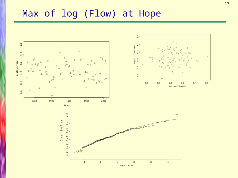
Max of log (Flow) at Hope
Years
Lo
g(m
ax.
flow
)
1920 1940 1960 1980 2000
8.6
8.8
9.0
9.2
9.4
9.6
Log(max.flow(i))
Lo
g(m
ax.
flow
)(i+
1)
8.6 8.8 9.0 9.2 9.4 9.6
8.6
8.8
9.0
9.2
9.4
9.6
Gumble.Q
Ord
er.
log
flo
w
-1 0 1 2 3 4
8.6
8.8
9.0
9.2
9.4
9.6
18
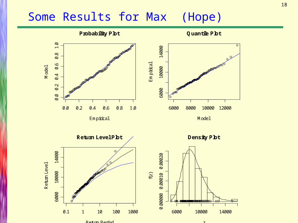
Some Results for Max (Hope)
0.0 0.2 0.4 0.6 0.8 1.0
0.0
0.2
0.4
0.6
0.8
1.0
Probability Plot
Empirical
Mod
el
6000 8000 10000 12000
6000
1000
014
000
Quantile Plot
Model
Em
piri
cal
6000
1000
014
000
Return Period
Ret
urn
Leve
l
0.1 1 10 100 1000
Return Level Plot Density Plot
z
f(z)
6000 10000 14000
0.00
000
0.00
010
0.00
020

19
Yearly maximum significant wave-height data 1949-1976
5.60 6.55 6.65 7.35 7.80 7.90 8.00 8.50 9.05 9.15 9.40 9.60 9.80 9.90 10.85 10.9011.10 11.30 11.30 11.55 11.75 12.85 12.90 13.40
1750 1800 1850 1900 1950 2000
Year
-10
010
20
Tem
p
Maximum and Minimum Tempertue for Basel 1755-1991
Two More Example: wave-height & Temperature (Basel)

20
Two Stations: Ratio of GEV Distributions W=X/(X+Y)

21
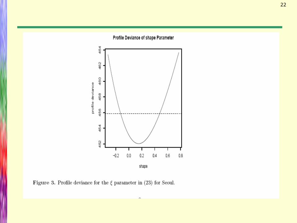
22

23
Seoul Rainfall Data

24
Current U.S. Environmental Protection Agency (USEPA) guidelines for:
a) designated beaches specify a 30-day geometric mean and a single-sample sample maximum corresponding to the 75th percentile based on that 30-day mean [USEPA, 1986].
b) drinking water specify the arithmetic mean coliform density of all standard samples examined per month shall not exceed one per 100ml.
EPA recent workshop to establish Recreational Water Quality Criteria, Chapel Hill, North Carolina last February: Objective was not only to determine compliance but also to relate waterborne illness to bacteriological indicator’s density
1. Estimation of Chemical Concentrations and Loadings (Ecosystem Health)
Microbiological Regulations (Human health)
25
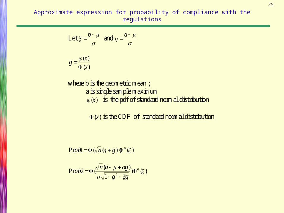
Approximate expression for probability of compliance with the regulations
Let
b and
a
)(
)(
x
xg
where b is the geometric mean ; a is single sample maximum )(x is the pdf of standard normal distribution
)(x is the CDF of standard normal distribution
)())((1Pr ngnob
)()1
)((2Pr
2
n
gg
ganob

26
Sample size n=5 and 10 # of simulations =10000

27
Ratio of single sample rejection probability to that of the mean rule (n = 5,10 and 20)
nagprob
bXprob nn
1
)(1log
)(1
)(1log
)(

28
14 16 18 20 22 24
0.0
0.1
0.2
0.3
Teperature
Pro
bab
ilit
y
Non- parametricGumbel
16 18 20 22
Temperature
0.0
0.2
0.4
0.6
0.8
Gu
mb
el
de
nsi
ty 1775- 18541775- 19911855- 1991
Figure 2. Fit ted Gumbel density for the full data and its two subsect ions
The Temperature Data: Change-Point
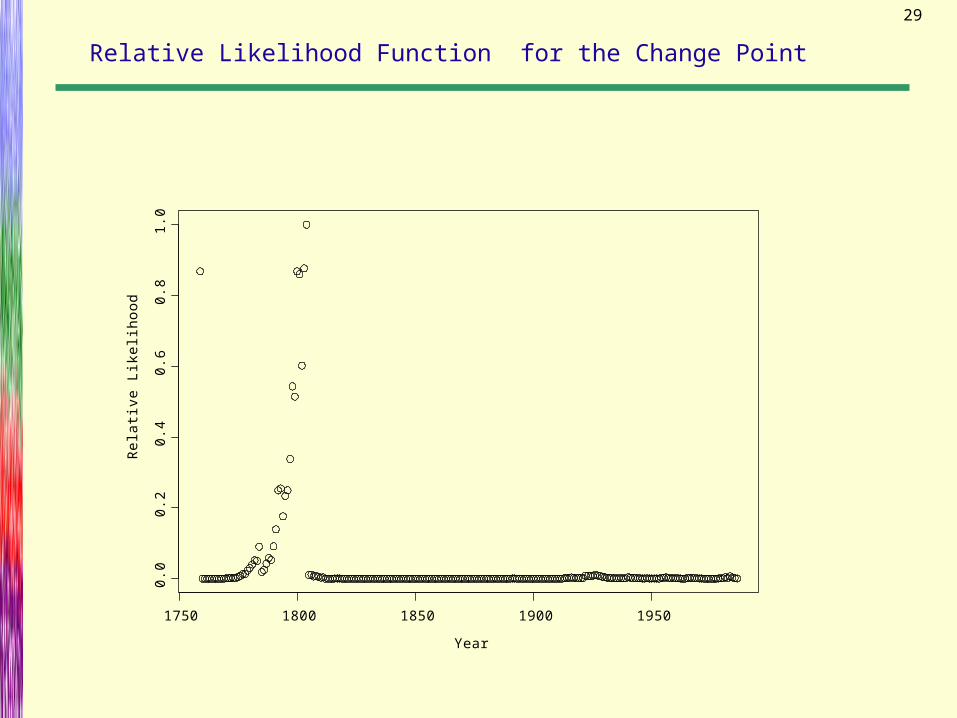
29
Relative Likelihood Function for the Change Point
Year
Re
lativ
e L
ike
liho
od
1750 1800 1850 1900 1950
0.0
0.2
0.4
0.6
0.8
1.0

30
Relative Likelihood function for the Change Point (Temp. Data)
x
f(x)
10 15 20 25 30
0.0
0.1
0.2
0.3
0.4
0.5
Segment1Segment2
Mu Sigma First segment 18.40425 0.7638125 Second segment 18.11343 1.301378 E(X) Var(X) First segment 18.84512 0.9596703 Second segment 18.86459 2.785836

31
Q-Q plots for the two segements
Theoritical Quantile
Obs
erve
d Q
uant
ile
-1 0 1 2 3 4
1819
20
Theoritical Quantile
Ob
se
rve
d Q
ua
ntile
0 2 4
16
18
20
22
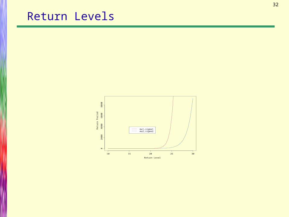
32
Return Levels
Return Level
Re
turn
Pe
rio
d
10 15 20 25 30
02
00
04
00
06
00
08
00
0
mu1,sigma1mu2,sigma2

33
Outline
• Some references
• Examples of extreme events data
• Types of extreme events data
• Commonly used models for extremes:
• Distributions of order statistics
• Generalized extreme value distributions
• Generalized Pareto distributions
• Parameter and quantile estimation of extremes
• Summary and concluding remarks

34
Types of Extreme Events Data
The choice of model and estimation methods depends on the type of available data.
Data, x1, x2, …, xn, drawn from a possibly unknown population, are available.
We wish to:1. Find an appropriate parametric model, F(x; ), that fits the data reasonably well
2. Estimate the parameters, and quantiles, X(p), of such a model

35
Types of Extreme Events Data
Examples:
1. Complete Data: All n observations are available.
Daily/Monthly energy consumption
•Daily/Monthly rain fall, stream discharge or flood flow

36
Types of Extreme Events Data
Examples:
2. Maxima/Minima: Only maxima or minima are available.
•Maximum/minimum daily/monthly temperatures
•Maximum daily/monthly wave heights
•Maximum daily/monthly wind speeds, pollution concentrations, etc.

37
Types of Extreme Events Data
3. Exceedances over/under a
threshold: When using yearly
maxima (minima), then an
important part of the information
large (small) values (other than the
two extremes occurring the same
year) is lost. The alternative is to
use the exceedances over (under) a
given threshold.

38
Exceedances Over/Under a Threshold
We are interested in events that cause
failure such as exceedances of a
random variable over a threshold
value.
For example, waves can destroy a
breakwater when their heights exceed
a given value, say 9 meters. Then it
does not matter whether the height of
a wave is 9.5, 10 or 12 meters
because the consequences of these
events are similar.

39
Exceedances Over/Under a Threshold
So, only failure causing observations
exceeding a given threshold are
available.
Definition:
Let X be a random variable and u be a
given threshold value. The event {X =
x} is said to be an exceedance at the
level u if X > u.

40
Summary: Types of Data
Extreme events data come in one of
three types:
1. Complete observations,
2. Maxima/Minima, or
3. Exceedances over/under a threshold
value
41
Outline
• Some references
• Examples of extreme events data
• Types of extreme events data
• Commonly used models for extremes:
• Distributions of order statistics
• Generalized extreme value distributions
• Generalized Pareto distributions
• Parameter and quantile estimation of extremes
• Summary and concluding remarks

42
Commonly Used Models for Extremes
The choice of model depends on the type of available data:
•Distributions of Order Statistics (DOS): Used when we have complete data
•Generalized Extreme Value (GEV) Distribution (AKA: Von Mises Family): Used for maxima/minima type of data
•Generalized Pareto Distribution (GPD): Used for exceedances over/under threshold type of data

43
Distributions of Order Statistics
Let X1, X2, …, Xn be a sample of size n
from a possibly unknown cdf F(x; ), depending on unknown vector-valued parameter .
Let X1:n < X2:n < … < Xn:n be the
corresponding order statistics.
Xi:n is called the ith order statistic.
Of particular interest is the minimum, X1:n, and the maximum, Xn:n order
statistics.

44
Distributions of Order Statistics
The distributions of the the order statistics are well know. For example:
• The cdf of the maximum order
statistics is:
• The cdf of the minimum order statistics is: nxFxF )()(min 11
nxFxF )()(max

45
Problems with Distributions of OS
The distributions of the order statistics have the following practical problems:
1. The cdf of the parent population, F(x; ), is usually unknown
2. When the data consist only of maxima or minima, the sample sizes are usually unknown
46
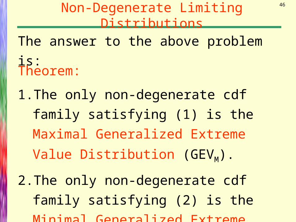
Non-Degenerate Limiting Distributions
The answer to the above problem is:
Theorem:
1. The only non-degenerate cdf family
satisfying (1) is the Maximal
Generalized Extreme Value
Distribution (GEVM).
2. The only non-degenerate cdf family
satisfying (2) is the Minimal
Generalized Extreme Value
Distribution (GEVm).

47Generalized Extreme Value Distributions
Thus, there are two GEV distributions,
one maximal, GEVM, and one minimal,
GEVm.
The GEV (AKA, Von Mises)
distributions were introduced by
Jenkinson (1955).
They are used when we have a large
sample or the observations
themselves are either minima or
maxima.
Their cdf are given later.

48Generalized Extreme Value Distributions
The GEV distributions are now widely
used to model extremes of natural and
environmental data. Examples are
found in: •Flood Studies Report of the USA’s
Natural Environment Research
Council (1975)
•Several articles in Tiago de Oliveira
(1984)
•Hosking, Wallis, and Wood (1985)
•Castillo et al. (2006)
49
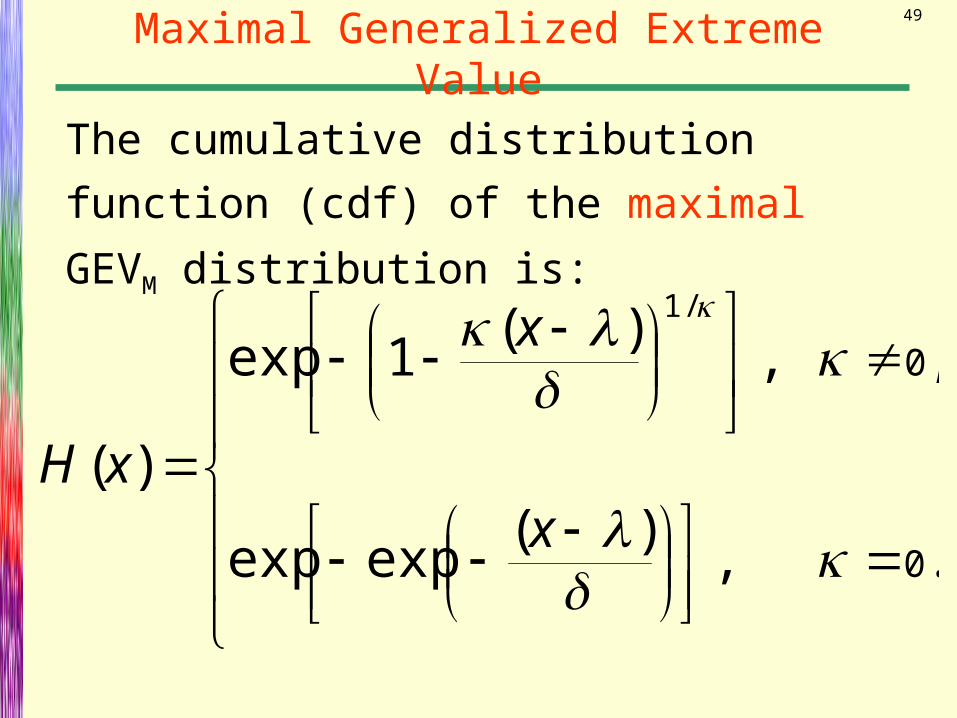
Maximal Generalized Extreme Value
The cumulative distribution function
(cdf) of the maximal GEVM distribution
is:
.,)(
expexp
,,)(
exp
)(
/
0
0
1
1
x
x
xH

50
Minimal Generalized Extreme Value
The cumulative distribution function
(cdf) of the minimal GEVm distribution
is:
.,)(
expexp
,,)(
exp
)(
/
0
0
1
111
x
x
xL

51
Relationship Between GEVM and GEVm
Theorem:
If the cdf of X is L(, , ), then the cdf
of Y = X is H(, , ).
Implication:
One form of the cdf can be obtained
from the other.

52
Maximal Generalized Extreme Value
The GEVM family has three-
parameters:
• is a location parameter
• is a scale parameter ( > 0)
• is a shape parameterThe parameter is the most important
of the three. The pth quantile is (0 < p
< 1): )log()/()( ppx 1
53
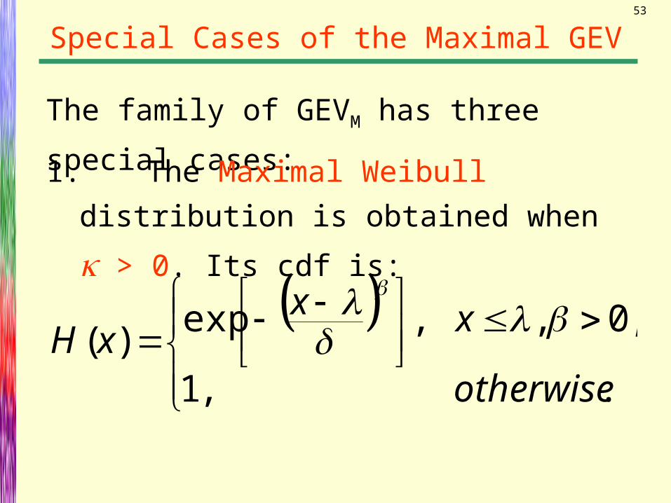
Special Cases of the Maximal GEV
The family of GEVM has three special
cases: 1. The Maximal Weibull distribution is
obtained when > 0. Its cdf is:
.,
,,,exp)(
otherwise
xxxH
1
0
54
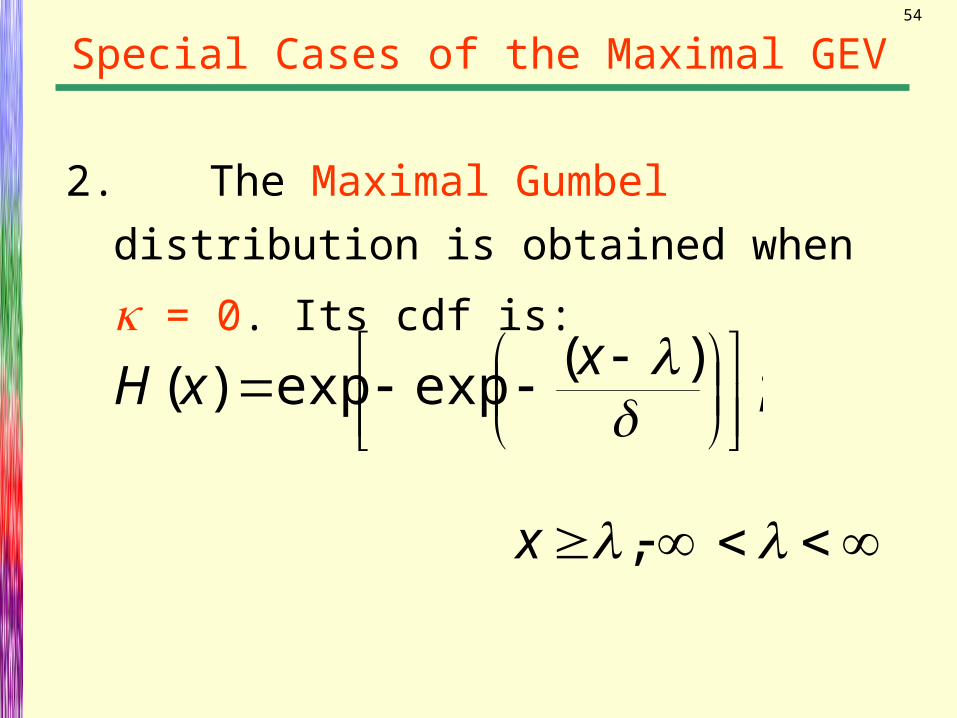
Special Cases of the Maximal GEV
2. The Maximal Gumbel distribution is
obtained when = 0. Its cdf is:
;)(
expexp)(
xxH
,x

55
Special Cases of the Maximal GEV
3. The Maximal Frechet distribution is
obtained when < 0. Its cdf is:
.,,exp
,,,)( 0
00
xx
xxH
56
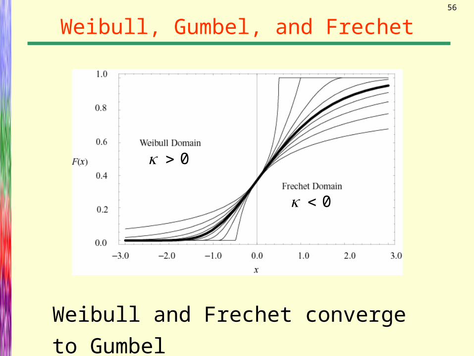
Weibull, Gumbel, and Frechet
Weibull and Frechet converge to
Gumbel
0
0

57
Summary
The GEV family can be used when:
1. The cdf of the parent population, F(x; ), is unknown
2. The sample size is very large (no degeneracy problems)
3. The data consist only of maxima or minima (we do not need to know the sample sizes)

58
Outline
• Some references
• Examples of extreme events data
• Types of extreme events data
• Commonly used models for extremes:
• Distributions of order statistics
• Generalized extreme value distributions
• Generalized Pareto distributions
• Parameter and quantile estimation of extremes
• Summary and concluding remarks

59
Types of Extreme Events Data
Recall the three types of extreme events data:
1. Complete Data: All n observations are available.
2. Maxima/Minima: Only maxima or minima are available
3. Exceedances over/under a threshold: Only observations exceeding a given threshold are available
Use distributions of order statistics if we know F(x) and n is not too large; else, use GEV.
Use distributions of order statistics if we know F(x) and n is not too large; else, use GEV.
Use GPD.Use GPD.
Use GEV.Use GEV.
60
Exceedances Over/Under a Threshold
As mentioned earlier, we are
interested in events that cause failure
such as exceedances of a random
variable over a threshold value.
The differences between the actual
values and the threshold value are
called exceedances over/under the
threshold.

61Generalized Maximal Pareto Distributions
Pickands (1975) demonstrates that
when the threshold tends to the upper
end of the random variable, the
exceedances follow a generalized
Pareto distribution, GPDM(, ), with
cdf
.,
,,/)(
/
/
0
0
1
11 1
xMe
xxF

62Generalized Maximal Pareto Distribution
The GPDM family has a two-
parameters:
• is a scale parameter ( > 0)
• is a shape parameter
The pth quantile is (0 < p < 1):
/)()( ppx 11
Note that when .)(Var,/ X21
63
Special Cases of the Maximal GPD
The GPDM has three special cases:
1. When = 0, the GPDM reduces to
the Exponential distribution with
mean .
2. When = 1, the GPDM reduces to
the Uniform U(0, ).
3. When < 0, the GPDM becomes the
Pareto distribution.

64Generalized Minimal Pareto Distribution
A similar family exists for the case of
exceedances under a threshold. These
are called the the Generalized Minimal
Pareto distributions or the Reversed
Generalized Pareto distributions.

65
Outline
• Some references
• Examples of extreme events data
• Types of extreme events data
• Commonly used models for extremes:
• Distributions of order statistics
• Generalized extreme value distributions
• Generalized Pareto distributions
• Parameter and quantile estimation of extremes
• Summary and concluding remarks

66
Parameter and Quantile Estimation
Available estimation methods include:
1. The maximum likelihood (MLE):
Jenkinson (1969)
Prescott and Walden (1980, 1983)
Smith (1984, 1985)
2. The method of moments (MOM)

67
Parameter and Quantile Estimation
3. The probability weighted moments (PWM):
Greenwood et al. (1979), Hosking et al. (1985)
4.The Elemental Percentile method (EPM): Castillo and Hadi (1995)
5.Order Statistics (Least Squares): El-Shaarawi
5. Modified Likelihood Function (MLF): El-Shaarawi and Hadi (work in progress).
68
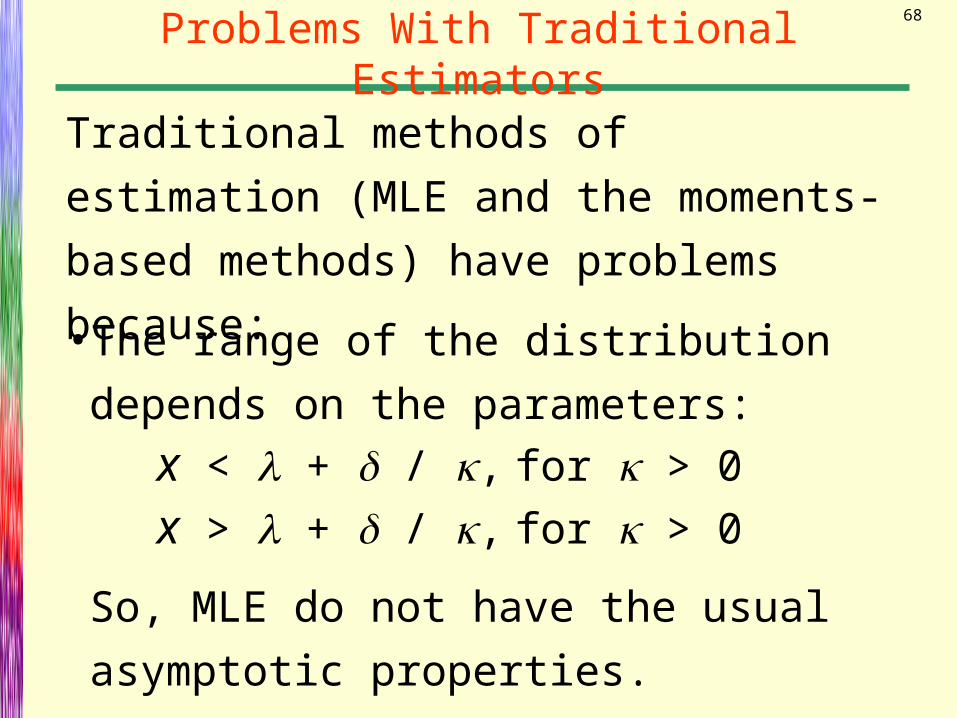
Problems With Traditional Estimators
Traditional methods of estimation
(MLE and the moments-based
methods) have problems because:
•The range of the distribution depends
on the parameters: x < + / , for > 0
x > + / , for > 0
So, MLE do not have the usual
asymptotic properties.
69
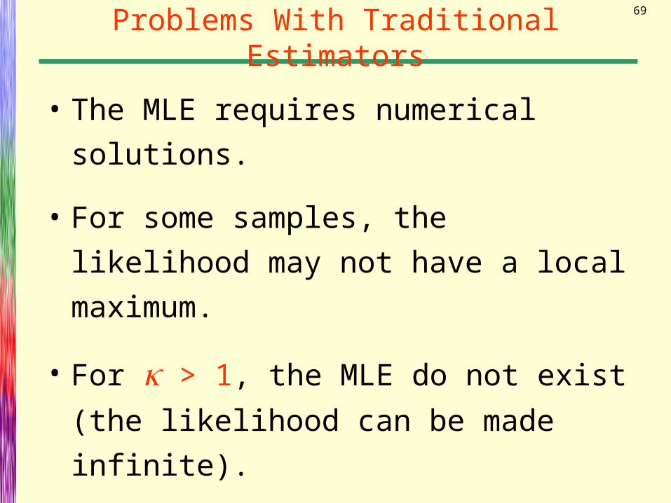
Problems With Traditional Estimators
• The MLE requires numerical
solutions.
• For some samples, the likelihood
may not have a local maximum.
• For > 1, the MLE do not exist (the
likelihood can be made infinite).

70
Problems With Traditional Estimators
• When < 1, the mean and higher
moments do not exist. So, MOM and
PWM do not exist when < 1.
• The PWM estimators are good for
cases where –0.5 < < 0.5.
• Outside this range of , the PWM
estimates may not exist, and if they do exist their performance worsens
as increases.
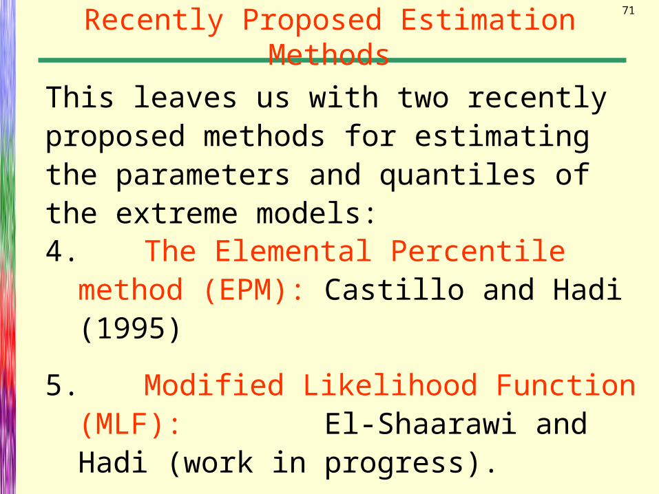
71Recently Proposed Estimation Methods
4. The Elemental Percentile method (EPM): Castillo and Hadi (1995)
5. Modified Likelihood Function (MLF): El-Shaarawi and Hadi (work in progress).
This leaves us with two recently proposed methods for estimating the parameters and quantiles of the extreme models:

72
Elemental Percentile method (EPM)
1. Initial estimates are obtained by equating three distinct order statistics to their corresponding percentiles:
nini pxF :: ),,;(
njnj pxF :: ),,;(
nrnr pxF :: ),,;(

73
Elemental Percentile method (EPM)
2. Substitute the cdf of the GEVM, we
obtain: )log()/( :: nini px 1
)log()/( :: njnj px 1
)log()/( :: nrnr px 1
These are three equations in three unknowns: , , and .
74
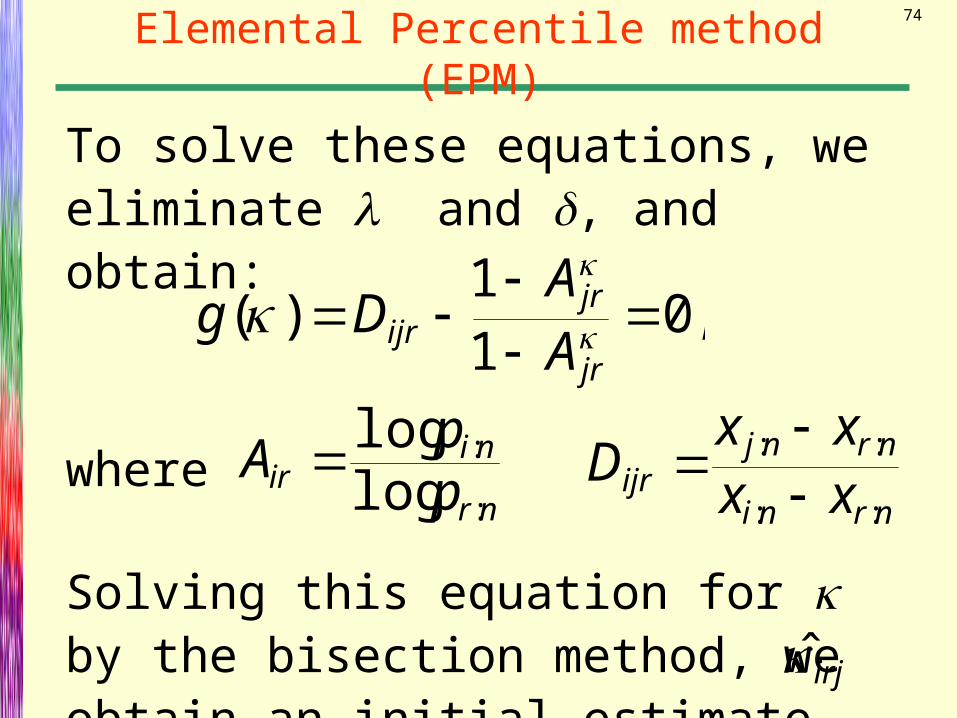
Elemental Percentile method (EPM)
To solve these equations, we eliminate and , and obtain:
,)( 011
jr
jrijr A
ADg
wherenr
niir p
pA
:
:
loglog
nrni
nrnjijr xx
xxD
::
::
Solving this equation for by the bisection method, we obtain an initial estimate .ˆirj

75
Elemental Percentile method (EPM)
Substituting in two of the above equations and solve for and :
irjirj
ninr
nrniirjijr
pp
xx
ˆ
:ˆ
:
::
loglog
ˆˆ
irj
irj
irjniirj
ijr
p
ˆ
ˆ:logˆ
ˆ
1
76
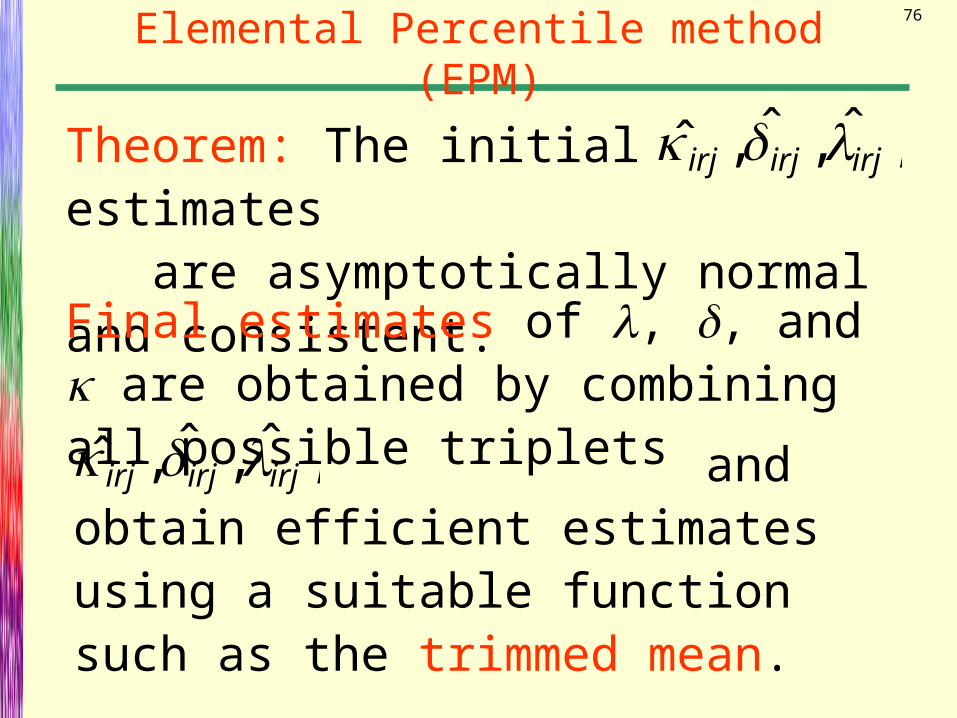
Elemental Percentile method (EPM)
Theorem: The initial estimates are asymptotically normal and consistent.
Final estimates of , , and are obtained by combining all possible triplets
,ˆ,ˆ,ˆ irjirjirj
and obtain efficient estimates using a suitable function such as the trimmed mean.
,ˆ,ˆ,ˆ irjirjirj
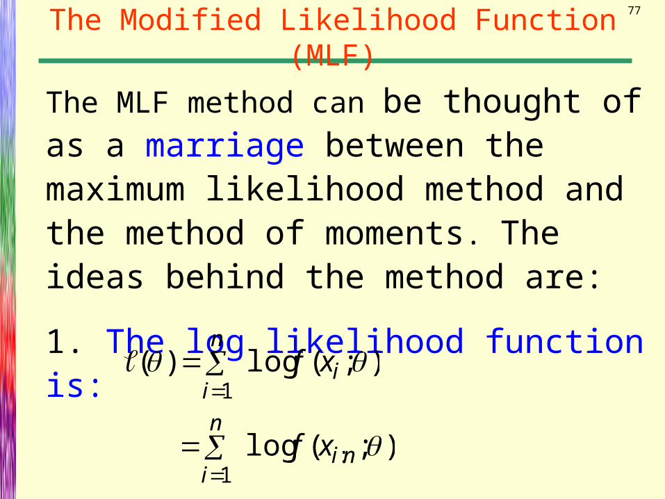
77The Modified Likelihood Function (MLF)
The MLF method can be thought of as a marriage between the maximum likelihood method and the method of moments. The ideas behind the method are:
1. The log likelihood function is:
);(log)(1
i
n
ixf
);(log :1
ni
n
ixf
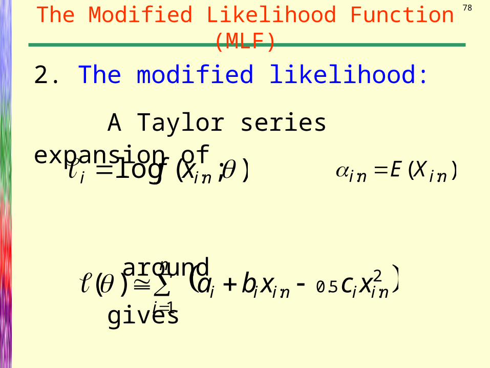
78The Modified Likelihood Function (MLF)
2. The modified likelihood:
A Taylor series expansion of
around
gives
);(log : nii xf )( :: nini XE
250
1niiniii
n
ixcxba :.:)(

79The Modified Likelihood Function (MLF)
3. Let )()( :: gXE nini
),;( :: nini pFX 1
where are plotting positions.
)/()(: bnaip ni
4. Substitute these in the modified likelihood and solve for .
80The Modified Likelihood Function (MLF)
We think this will be a happy marriage, but to be sure we are:
Investigating (analytically and using simulation) the properties of the proposed estimators and their dependence on the choice of the plotting positions pi:n.
This is still work in progress.

81
Outline
• Some references
• Examples of extreme events data
• Types of extreme events data
• Commonly used models for extremes:
• Distributions of order statistics
• Generalized extreme value distributions
• Generalized Pareto distributions
• Parameter and quantile estimation of extremes
• Summary and concluding remarks
82
Summary
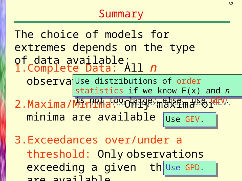
The choice of models for extremes depends on the type of data available:1. Complete Data: All n observations
are available.
2. Maxima/Minima: Only maxima or minima are available
3. Exceedances over/under a threshold: Only observations exceeding a given threshold are available
Use GPD.Use GPD.
Use GEV.Use GEV.
Use distributions of order statistics if we know F(x) and n is not too large; else, use GEV.
Use distributions of order statistics if we know F(x) and n is not too large; else, use GEV.