a very nice overview -

Performance Attribution from Bacon

Matthieu Lestel

August 19, 2012

Abstract

This vignette gives a brief overview of the functions developed in Bacon(2008) toevaluate the performance and risk of portfolios that are included in PerformanceAn-alytics and how to use them. There are some tables at the end which give a quickoverview of similar functions. The page number next to each function is the locationof the function in Bacon(2008)

Contents

1 Risk Measure 31.1 Mean absolute deviation (p.62) . . . . . . . . . . . . . . . . . . . . . . . . 31.2 Frequency (p.64) . . . . . . . . . . . . . . . . . . . . . . . . . . . . . . . . 31.3 Sharpe Ratio (p.64) . . . . . . . . . . . . . . . . . . . . . . . . . . . . . . . 41.4 Risk-adjusted return: MSquared (p.67) . . . . . . . . . . . . . . . . . . . . 41.5 MSquared Excess (p.68) . . . . . . . . . . . . . . . . . . . . . . . . . . . . 4

2 Regression analysis 52.1 Regression equation (p.71) . . . . . . . . . . . . . . . . . . . . . . . . . . . 52.2 Regression alpha (p.71) . . . . . . . . . . . . . . . . . . . . . . . . . . . . . 52.3 Regression beta (p.71) . . . . . . . . . . . . . . . . . . . . . . . . . . . . . 52.4 Regression epsilon (p.71) . . . . . . . . . . . . . . . . . . . . . . . . . . . . 62.5 Jensen’s alpha (p.72) . . . . . . . . . . . . . . . . . . . . . . . . . . . . . . 62.6 Systematic Risk (p.75) . . . . . . . . . . . . . . . . . . . . . . . . . . . . . 62.7 Specific Risk (p.75) . . . . . . . . . . . . . . . . . . . . . . . . . . . . . . . 72.8 Total Risk (p.75) . . . . . . . . . . . . . . . . . . . . . . . . . . . . . . . . 72.9 Treynor ratio (p.75) . . . . . . . . . . . . . . . . . . . . . . . . . . . . . . . 72.10 Modified Treynor ratio (p.77) . . . . . . . . . . . . . . . . . . . . . . . . . 72.11 Appraisal ratio (or Treynor-Black ratio) (p.77) . . . . . . . . . . . . . . . . 82.12 Modified Jensen (p.77) . . . . . . . . . . . . . . . . . . . . . . . . . . . . . 8

1

2.13 Fama decomposition (p.77) . . . . . . . . . . . . . . . . . . . . . . . . . . . 82.14 Selectivity (p.78) . . . . . . . . . . . . . . . . . . . . . . . . . . . . . . . . 92.15 Net selectivity (p.78) . . . . . . . . . . . . . . . . . . . . . . . . . . . . . . 9

3 Relative Risk 93.1 Tracking error (p.78) . . . . . . . . . . . . . . . . . . . . . . . . . . . . . . 93.2 Information ratio (p.80) . . . . . . . . . . . . . . . . . . . . . . . . . . . . 10

4 Return Distribution 104.1 Skewness (p.83) . . . . . . . . . . . . . . . . . . . . . . . . . . . . . . . . . 104.2 Sample skewness (p.84) . . . . . . . . . . . . . . . . . . . . . . . . . . . . . 104.3 Kurtosis (p.84) . . . . . . . . . . . . . . . . . . . . . . . . . . . . . . . . . 114.4 Excess kurtosis (p.85) . . . . . . . . . . . . . . . . . . . . . . . . . . . . . . 114.5 Sample kurtosis (p.85) . . . . . . . . . . . . . . . . . . . . . . . . . . . . . 114.6 Sample excess kurtosis (p.85) . . . . . . . . . . . . . . . . . . . . . . . . . 12

5 Drawdown 125.1 Pain index (p.89) . . . . . . . . . . . . . . . . . . . . . . . . . . . . . . . . 125.2 Calmar ratio (p.89) . . . . . . . . . . . . . . . . . . . . . . . . . . . . . . . 125.3 Sterling ratio (p.89) . . . . . . . . . . . . . . . . . . . . . . . . . . . . . . . 135.4 Burke ratio (p.90) . . . . . . . . . . . . . . . . . . . . . . . . . . . . . . . . 135.5 Modified Burke ratio (p.91) . . . . . . . . . . . . . . . . . . . . . . . . . . 135.6 Martin ratio (p.91) . . . . . . . . . . . . . . . . . . . . . . . . . . . . . . . 145.7 Pain ratio (p.91) . . . . . . . . . . . . . . . . . . . . . . . . . . . . . . . . 14

6 Downside risk 146.1 Downside risk (p.92) . . . . . . . . . . . . . . . . . . . . . . . . . . . . . . 146.2 UpsideRisk (p.92) . . . . . . . . . . . . . . . . . . . . . . . . . . . . . . . . 156.3 Downside frequency (p.94) . . . . . . . . . . . . . . . . . . . . . . . . . . . 166.4 Bernardo and Ledoit ratio (p.95) . . . . . . . . . . . . . . . . . . . . . . . 166.5 d ratio (p.95) . . . . . . . . . . . . . . . . . . . . . . . . . . . . . . . . . . 176.6 Omega-Sharpe ratio (p.95) . . . . . . . . . . . . . . . . . . . . . . . . . . . 176.7 Sortino ratio (p.96) . . . . . . . . . . . . . . . . . . . . . . . . . . . . . . . 186.8 Kappa (p.96) . . . . . . . . . . . . . . . . . . . . . . . . . . . . . . . . . . 186.9 Upside potential ratio (p.97) . . . . . . . . . . . . . . . . . . . . . . . . . . 186.10 Volatility skewness (p.97) . . . . . . . . . . . . . . . . . . . . . . . . . . . 196.11 Variability skewness (p.98) . . . . . . . . . . . . . . . . . . . . . . . . . . . 196.12 Adjusted Sharpe ratio (p.99) . . . . . . . . . . . . . . . . . . . . . . . . . . 206.13 Skewness-kurtosis ratio (p.99) . . . . . . . . . . . . . . . . . . . . . . . . . 206.14 Prospect ratio (p.100) . . . . . . . . . . . . . . . . . . . . . . . . . . . . . 20

2

7 Return adjusted for downside risk 217.1 M Squared for Sortino (p.102) . . . . . . . . . . . . . . . . . . . . . . . . . 217.2 Omega excess return (p.103) . . . . . . . . . . . . . . . . . . . . . . . . . . 21

8 Tables 218.1 Variability risk . . . . . . . . . . . . . . . . . . . . . . . . . . . . . . . . . 218.2 Specific risk . . . . . . . . . . . . . . . . . . . . . . . . . . . . . . . . . . . 228.3 Information risk . . . . . . . . . . . . . . . . . . . . . . . . . . . . . . . . . 228.4 Distributions . . . . . . . . . . . . . . . . . . . . . . . . . . . . . . . . . . 238.5 Drawdowns . . . . . . . . . . . . . . . . . . . . . . . . . . . . . . . . . . . 238.6 Downside risk . . . . . . . . . . . . . . . . . . . . . . . . . . . . . . . . . . 248.7 Sharpe ratio . . . . . . . . . . . . . . . . . . . . . . . . . . . . . . . . . . . 24

1 Risk Measure

1.1 Mean absolute deviation (p.62)

To calculate Mean absolute deviation we take the sum of the absolute value of the differencebetween the returns and the mean of the returns and we divide it by the number of returns.

MeanAbsoluteDeviation =

∑ni=1 | ri − r |

n

where ns the number of observations of the entire series, ris the return in month i andrs the mean return

> #data(portfolio_bacon)

> print(MeanAbsoluteDeviation(portfolio_bacon[,1])) #expected 0.0310

[1] 0.03108333

1.2 Frequency (p.64)

Gives the period of the return distribution (ie 12 if monthly return, 4 if quarterly return)


> print(Frequency(portfolio_bacon[,1])) #expected 12

[1] 12

3

1.3 Sharpe Ratio (p.64)

The Sharpe ratio is simply the return per unit of risk (represented by variability). In theclassic case, the unit of risk is the standard deviation of the returns.

(Ra −Rf )√σ(Ra−Rf )

> data(managers)

> SharpeRatio(managers[,1,drop=FALSE], Rf=.035/12, FUN="StdDev")

HAM1

StdDev Sharpe (Rf=0.3%, p=95%): 0.3201889

1.4 Risk-adjusted return: MSquared (p.67)

M2s a risk adjusted return useful to judge the size of relative performance between differ-ents portfolios. With it you can compare portfolios with different levels of risk.

M2 = rP + SR ∗ (σM − σP ) = (rP − rF ) ∗ σMσP

+ rF

where rP is the portfolio return annualized, σM is the market risk and σP s the portfoliorisk


> print(MSquared(portfolio_bacon[,1], portfolio_bacon[,2])) #expected 0.1068

portfolio.monthly.return....

portfolio.monthly.return.... 0.1068296

1.5 MSquared Excess (p.68)

M2xcess is the quantity above the standard M. There is a geometric excess return whichis better for Bacon and an arithmetic excess return

M2excess(geometric) =1 +M2

1 + b− 1

M2excess(arithmetic) = M2 − bwhere M2 is MSquared and b is the benchmark annualised return.


> print(MSquaredExcess(portfolio_bacon[,1], portfolio_bacon[,2])) #expected -0.00998

4


portfolio.monthly.return.... -0.009976721

> print(MSquaredExcess(portfolio_bacon[,1], portfolio_bacon[,2], Method="arithmetic")) #expected -0.011



2 Regression analysis

2.1 Regression equation (p.71)

rP = α + β ∗ b+ ε

2.2 Regression alpha (p.71)

”Alpha” purports to be a measure of a manager’s skill by measuring the portion of themanagers returns that are not attributable to ”Beta”, or the portion of performance at-tributable to a benchmark.

> #data(managers)

> print(CAPM.alpha(managers[,1,drop=FALSE], managers[,8,drop=FALSE], Rf=.035/12))

[1] 0.005960609

2.3 Regression beta (p.71)

CAPM Beta is the beta of an asset to the variance and covariance of an initial portfolio.Used to determine diversification potential.

> #data(managers)

> CAPM.beta(managers[, "HAM2", drop=FALSE], managers[, "SP500 TR", drop=FALSE], Rf = managers[, "US 3m TR", drop=FALSE])

[1] 0.3383942

5

2.4 Regression epsilon (p.71)

The regression epsilon is an error term measuring the vertical distance between the returnpredicted by the equation and the real result.

εr = rp − αr − βr ∗ b

where αrs the regression alpha, βrs the regression beta, rps the portfolio return and bis the benchmark return

> #data(managers)

> print(CAPM.epsilon(portfolio_bacon[,1], portfolio_bacon[,2])) #expected -0.013

[1] -0.01313932

2.5 Jensen’s alpha (p.72)

The Jensen’s alpha is the intercept of the regression equation in the Capital Asset PricingModel and is in effect the exess return adjusted for systematic risk.

α = rp − rf − βp ∗ (b− rf )

where rf is the risk free rate, βr is the regression beta, rp is the portfolio return and bis the benchmark return


> print(CAPM.jensenAlpha(portfolio_bacon[,1], portfolio_bacon[,2])) #expected -0.014

[1] -0.01416944

2.6 Systematic Risk (p.75)

Systematic risk as defined by Bacon(2008) is the product of beta by market risk. Becareful ! It’s not the same definition as the one given by Michael Jensen. Market risk isthe standard deviation of the benchmark. The systematic risk is annualized

σs = β ∗ σm

where σs is the systematic risk, β is the regression beta, and σms the market risk


> print(SystematicRisk(portfolio_bacon[,1], portfolio_bacon[,2])) #expected 0.013

[1] 0.1300098

6

2.7 Specific Risk (p.75)

Specific risk is the standard deviation of the error term in the regression equation.


> print(SpecificRisk(portfolio_bacon[,1], portfolio_bacon[,2])) #expected 0.0329

[1] 0.03293109

2.8 Total Risk (p.75)

The square of total risk is the sum of the square of systematic risk and the square ofspecific risk. Specific risk is the standard deviation of the error term in the regressionequation. Both terms are annualized to calculate total risk.

TotalRisk =√SystematicRisk2 + SpecificRisk2


> print(TotalRisk(portfolio_bacon[,1], portfolio_bacon[,2])) #expected 0.0134

[1] 0.1341156

2.9 Treynor ratio (p.75)

The Treynor ratio is similar to the Sharpe Ratio, except it uses beta as the volatilitymeasure (to divide the investment’s excess return over the beta).

TreynorRatio =(Ra −Rf )

βa,b

> #data(managers)

> print(round(TreynorRatio(managers[,1,drop=FALSE], managers[,8,drop=FALSE], Rf=.035/12),4))

[1] 0.2528

2.10 Modified Treynor ratio (p.77)

To calculate modified Treynor ratio, we divide the numerator by the systematic risk insteadof the beta.


> print(TreynorRatio(portfolio_bacon[,1], portfolio_bacon[,2], modified = TRUE)) #expected 1.677

[1] 0.7974653

7

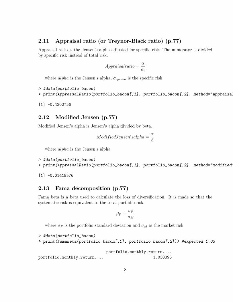
2.11 Appraisal ratio (or Treynor-Black ratio) (p.77)

Appraisal ratio is the Jensen’s alpha adjusted for specific risk. The numerator is dividedby specific risk instead of total risk.

Appraisalratio =α

σε

where alpha is the Jensen’s alpha, σepsilon is the specific risk


> print(AppraisalRatio(portfolio_bacon[,1], portfolio_bacon[,2], method="appraisal")) #expected -0.430

[1] -0.4302756

2.12 Modified Jensen (p.77)

Modified Jensen’s alpha is Jensen’s alpha divided by beta.

ModifiedJensen′salpha =α

β

where alpha is the Jensen’s alpha


> print(AppraisalRatio(portfolio_bacon[,1], portfolio_bacon[,2], method="modified"))

[1] -0.01418576

2.13 Fama decomposition (p.77)

Fama beta is a beta used to calculate the loss of diversification. It is made so that thesystematic risk is equivalent to the total portfolio risk.

βF =σPσM

where σP is the portfolio standard deviation and σM is the market risk


> print(FamaBeta(portfolio_bacon[,1], portfolio_bacon[,2])) #expected 1.03


portfolio.monthly.return.... 1.030395

8

2.14 Selectivity (p.78)

Selectivity is the same as Jensen’s alpha

Selectivity = rp − rf − βp ∗ (b− rf )where rf is the risk free rate, βr is the regression beta, rp is the portfolio return and b

is the benchmark return


> print(Selectivity(portfolio_bacon[,1], portfolio_bacon[,2])) #expected -0.0141

[1] -0.01416944

2.15 Net selectivity (p.78)

Net selectivity is the remaining selectivity after deducting the amount of return require tojustify not being fully diversified

If net selectivity is negative the portfolio manager has not justified the loss of diversi-fication

Netselectivity = α− dwhere α is the selectivity and d is the diversification


> print(NetSelectivity(portfolio_bacon[,1], portfolio_bacon[,2])) #expected -0.017



3 Relative Risk

3.1 Tracking error (p.78)

A measure of the unexplained portion of performance relative to a benchmark.Tracking error is calculated by taking the square root of the average of the squared

deviations between the investment’s returns and the benchmark’s returns, then multiplyingthe result by the square root of the scale of the returns.

TrackingError =

√√√√∑ (Ra −Rb)2

len(Ra)√scale

> #data(managers)

> TrackingError(managers[,1,drop=FALSE], managers[,8,drop=FALSE])

[1] 0.1131667

9

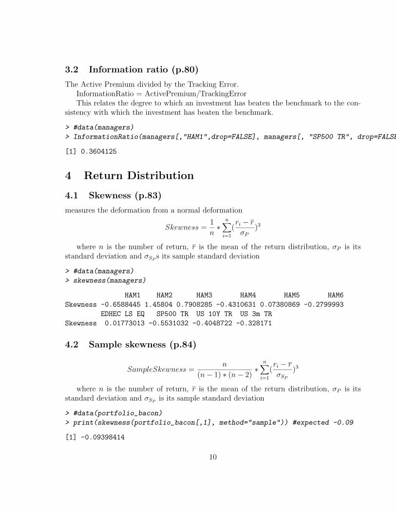
3.2 Information ratio (p.80)

The Active Premium divided by the Tracking Error.InformationRatio = ActivePremium/TrackingErrorThis relates the degree to which an investment has beaten the benchmark to the con-

sistency with which the investment has beaten the benchmark.

> #data(managers)

> InformationRatio(managers[,"HAM1",drop=FALSE], managers[, "SP500 TR", drop=FALSE])

[1] 0.3604125

4 Return Distribution

4.1 Skewness (p.83)

measures the deformation from a normal deformation

Skewness =1

n∗

n∑i=1

(ri − rσP

)3

where n is the number of return, r is the mean of the return distribution, σP is itsstandard deviation and σSP

s its sample standard deviation

> #data(managers)

> skewness(managers)

HAM1 HAM2 HAM3 HAM4 HAM5 HAM6

Skewness -0.6588445 1.45804 0.7908285 -0.4310631 0.07380869 -0.2799993

EDHEC LS EQ SP500 TR US 10Y TR US 3m TR

Skewness 0.01773013 -0.5531032 -0.4048722 -0.328171

4.2 Sample skewness (p.84)

SampleSkewness =n

(n− 1) ∗ (n− 2)∗

n∑i=1

(ri − rσSP

)3


is its sample standard deviation


> print(skewness(portfolio_bacon[,1], method="sample")) #expected -0.09

[1] -0.09398414

10

4.3 Kurtosis (p.84)

Kurtosis measures the weight or returns in the tails of the distribution relative to standarddeviation.

Kurtosis(moment) =1

n∗

n∑i=1

(ri − rσP

)4




> print(kurtosis(portfolio_bacon[,1], method="moment")) #expected 2.43

[1] 2.432454

4.4 Excess kurtosis (p.85)

ExcessKurtosis =1

n∗

n∑i=1

(ri − rσP

)4 − 3




> print(kurtosis(portfolio_bacon[,1], method="excess")) #expected -0.57

[1] -0.5675462

4.5 Sample kurtosis (p.85)

Samplekurtosis =n ∗ (n+ 1)

(n− 1) ∗ (n− 2) ∗ (n− 3)∗

n∑i=1

(ri − rσSP

)4




> print(kurtosis(portfolio_bacon[,1], method="sample")) #expected 3.03

[1] 3.027405

11

4.6 Sample excess kurtosis (p.85)

Sampleexcesskurtosis =n ∗ (n+ 1)

(n− 1) ∗ (n− 2) ∗ (n− 3)∗

n∑i=1

(ri − rσSP

)4 − 3 ∗ (n− 1)2

(n− 2) ∗ (n− 3)




> print(kurtosis(portfolio_bacon[,1], method="sample_excess")) #expected -0.41

[1] -0.4076603

5 Drawdown

5.1 Pain index (p.89)

The pain index is the mean value of the drawdowns over the entire analysis period. Themeasure is similar to the Ulcer index except that the drawdowns are not squared. Also,it’s different than the average drawdown, in that the numerator is the total number ofobservations rather than the number of drawdowns. Visually, the pain index is the areaof the region that is enclosed by the horizontal line at zero percent and the drawdown linein the Drawdown chart.

Painindex =n∑i=1

| D′i |n

where n is the number of observations of the entire series, D′i is the drawdown sinceprevious peak in period i


> print(PainIndex(portfolio_bacon[,1])) #expected 0.04


Pain Index 0.0390113

5.2 Calmar ratio (p.89)

Calmar ratio is another method of creating a risk-adjusted measure for ranking investmentssimilar to the Sharpe ratio.

> #data(managers)

> CalmarRatio(managers[,1,drop=FALSE])

HAM1

Calmar Ratio 0.9061697

12

5.3 Sterling ratio (p.89)

Sterling ratio is another method of creating a risk-adjusted measure for ranking investmentssimilar to the Sharpe ratio.

> #data(managers)

> SterlingRatio(managers[,1,drop=FALSE])

HAM1

Sterling Ratio (Excess = 10%) 0.5462542

5.4 Burke ratio (p.90)

To calculate Burke ratio we take the difference between the portfolio return and the riskfree rate and we divide it by the square root of the sum of the square of the drawdowns.

BurkeRatio =rP − rF√∑d

t=1Dt2

where d is number of drawdowns, rP s the portfolio return, rF is the risk free rate andDt the tthrawdown.


> print(BurkeRatio(portfolio_bacon[,1])) #expected 0.74

[1] 0.7447309

5.5 Modified Burke ratio (p.91)

To calculate the modified Burke ratio we just multiply the Burke ratio by the square rootof the number of datas.

ModifiedBurkeRatio =rP − rF√∑d

t=1Dt

2

n

where n is the number of observations of the entire series, ds number of drawdowns,rP is the portfolio return, rF is the risk free rate and Dt the tth drawdown.


> print(BurkeRatio(portfolio_bacon[,1], modified = TRUE)) #expected 3.65

[1] 3.648421

13

5.6 Martin ratio (p.91)

To calculate Martin ratio we divide the difference of the portfolio return and the risk freerate by the Ulcer index

Martinratio =rP − rF√∑n

i=1D′

i2

n

where rP is the annualized portfolio return, rF is the risk free rate, n is the number ofobservations of the entire series, D′i is the drawdown since previous peak in period i


> print(MartinRatio(portfolio_bacon[,1])) #expected 1.70


Ulcer Index 1.70772

5.7 Pain ratio (p.91)

To calculate Pain ratio we divide the difference of the portfolio return and the risk freerate by the Pain index

Painratio =rP − rF∑ni=1

|D′i|n

where rP is the annualized portfolio return, rF is the risk free rate, n is the number ofobservations of the entire series, D′i is the drawdown since previous peak in period i


> print(PainRatio(portfolio_bacon[,1])) #expected 2.66


Pain Index 2.657647

6 Downside risk

6.1 Downside risk (p.92)

Downside deviation, similar to semi deviation, eliminates positive returns when calculatingrisk. Instead of using the mean return or zero, it uses the Minimum Acceptable Return asproposed by Sharpe (which may be the mean historical return or zero). It measures the

14

variability of underperformance below a minimum targer rate. The downside variance isthe square of the downside potential.

DownsideDeviation(R,MAR) = δMAR =

√√√√ n∑t=1

min[(Rt −MAR), 0]2

n

DownsideV ariance(R,MAR) =n∑t=1

min[(Rt −MAR), 0]2

n

DownsidePotential(R,MAR) =n∑t=1

min[(Rt −MAR), 0]

n

where n is either the number of observations of the entire series or the number ofobservations in the subset of the series falling below the MAR.


> MAR = 0.5

> DownsideDeviation(portfolio_bacon[,1], MAR) #expected 0.493

[1] 0.492524

> DownsidePotential(portfolio_bacon[,1], MAR) #expected 0.491

[1] 0.491

6.2 UpsideRisk (p.92)

Upside Risk is the similar of semideviation taking the return above the Minimum Accept-able Return instead of using the mean return or zero.

UpsideRisk(R,MAR) =

√√√√ n∑t=1

max[(Rt −MAR), 0]2

n

UpsideV ariance(R,MAR) =n∑t=1

max[(Rt −MAR), 0]2

n

UpsidePotential(R,MAR) =n∑t=1

max[(Rt −MAR), 0]

n

where n is either the number of observations of the entire series or the number ofobservations in the subset of the series falling below the MAR.

15


> MAR = 0.005

> print(UpsideRisk(portfolio_bacon[,1], MAR, stat="risk")) #expected 0.02937

[1] 0.02937332

> print(UpsideRisk(portfolio_bacon[,1], MAR, stat="variance")) #expected 0.08628

[1] 0.0008627917

> print(UpsideRisk(portfolio_bacon[,1], MAR, stat="potential")) #expected 0.01771

[1] 0.01770833

6.3 Downside frequency (p.94)

To calculate Downside Frequency, we take the subset of returns that are less than thetarget (or Minimum Acceptable Returns (MAR)) returns and divide the length of thissubset by the total number of returns.

DownsideFrequency(R,MAR) =n∑t=1

min[(Rt −MAR), 0]

Rt ∗ n

where n is the number of observations of the entire series


> MAR = 0.005

> print(DownsideFrequency(portfolio_bacon[,1], MAR)) #expected 0.458

[1] 0.4583333

6.4 Bernardo and Ledoit ratio (p.95)

To calculate Bernardo and Ledoit ratio we take the sum of the subset of returns that areabove 0 and we divide it by the opposite of the sum of the subset of returns that are below0

BernardoLedoitRatio(R) =1n

∑nt=1max(Rt, 0)

1n

∑nt=1max(−Rt, 0)



> print(BernardoLedoitRatio(portfolio_bacon[,1])) #expected 1.78

[1] 1.779783

16

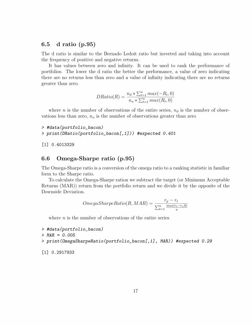
6.5 d ratio (p.95)

The d ratio is similar to the Bernado Ledoit ratio but inverted and taking into accountthe frequency of positive and negative returns.

It has values between zero and infinity. It can be used to rank the performance ofportfolios. The lower the d ratio the better the performance, a value of zero indicatingthere are no returns less than zero and a value of infinity indicating there are no returnsgreater than zero.

DRatio(R) =nd ∗

∑nt=1max(−Rt, 0)

nu ∗∑nt=1max(Rt, 0)

where n is the number of observations of the entire series, nd is the number of obser-vations less than zero, nu is the number of observations greater than zero


> print(DRatio(portfolio_bacon[,1])) #expected 0.401

[1] 0.4013329

6.6 Omega-Sharpe ratio (p.95)

The Omega-Sharpe ratio is a conversion of the omega ratio to a ranking statistic in familiarform to the Sharpe ratio.

To calculate the Omega-Sharpe ration we subtract the target (or Minimum AcceptableReturns (MAR)) return from the portfolio return and we divide it by the opposite of theDownside Deviation.

OmegaSharpeRatio(R,MAR) =rp − rt∑n

t=1max(rt−ri,0)

n



> MAR = 0.005

> print(OmegaSharpeRatio(portfolio_bacon[,1], MAR)) #expected 0.29

[1] 0.2917933

17

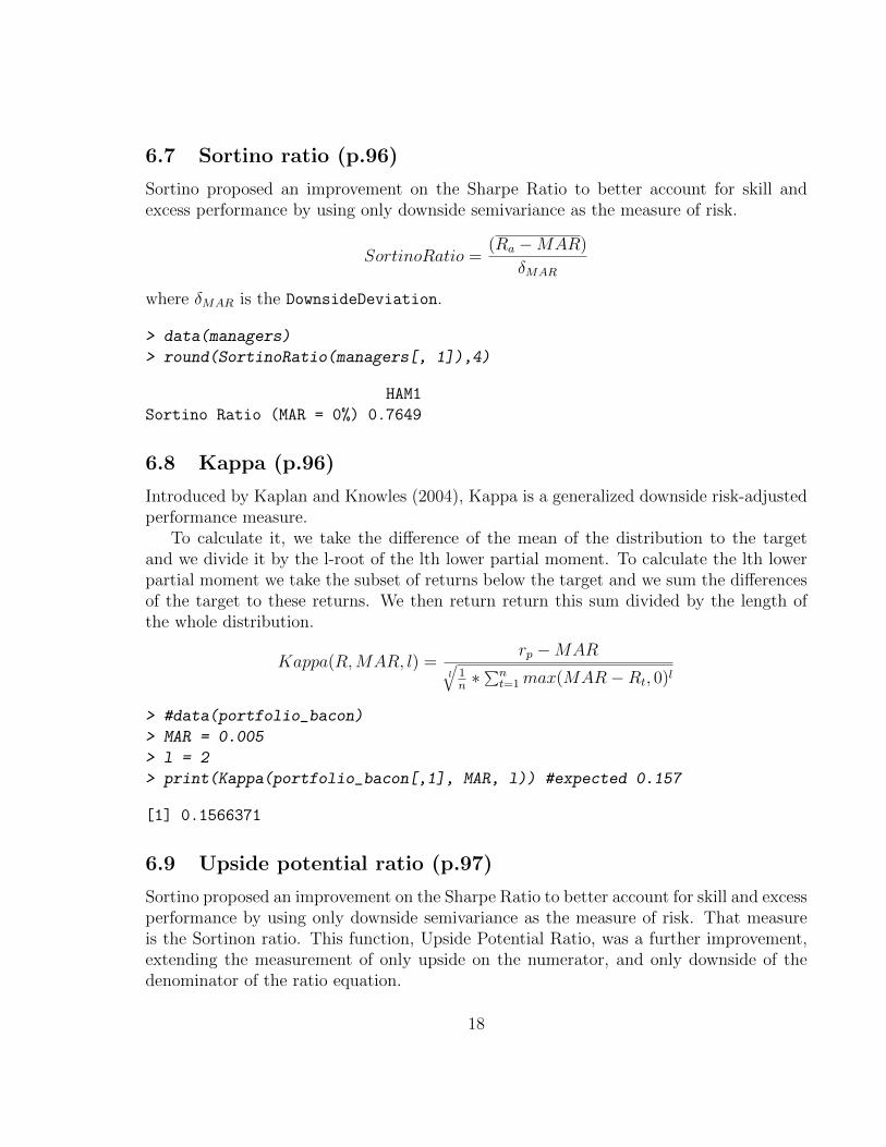
6.7 Sortino ratio (p.96)

Sortino proposed an improvement on the Sharpe Ratio to better account for skill andexcess performance by using only downside semivariance as the measure of risk.

SortinoRatio =(Ra −MAR)

δMAR

where δMAR is the DownsideDeviation.

> data(managers)

> round(SortinoRatio(managers[, 1]),4)

HAM1

Sortino Ratio (MAR = 0%) 0.7649

6.8 Kappa (p.96)

Introduced by Kaplan and Knowles (2004), Kappa is a generalized downside risk-adjustedperformance measure.

To calculate it, we take the difference of the mean of the distribution to the targetand we divide it by the l-root of the lth lower partial moment. To calculate the lth lowerpartial moment we take the subset of returns below the target and we sum the differencesof the target to these returns. We then return return this sum divided by the length ofthe whole distribution.

Kappa(R,MAR, l) =rp −MAR

l

√1n∗∑n

t=1max(MAR−Rt, 0)l


> MAR = 0.005

> l = 2

> print(Kappa(portfolio_bacon[,1], MAR, l)) #expected 0.157

[1] 0.1566371

6.9 Upside potential ratio (p.97)

Sortino proposed an improvement on the Sharpe Ratio to better account for skill and excessperformance by using only downside semivariance as the measure of risk. That measureis the Sortinon ratio. This function, Upside Potential Ratio, was a further improvement,extending the measurement of only upside on the numerator, and only downside of thedenominator of the ratio equation.

18

UPR =

∑nt=1(Rt −MAR)

δMAR

where δMAR is the DownsideDeviation.

> data(edhec)

> UpsidePotentialRatio(edhec[, 6], MAR=.05/12) #5 percent/yr MAR

Event Driven

Upside Potential (MAR = 0.4%) 0.5376613

6.10 Volatility skewness (p.97)

Volatility skewness is a similar measure to omega but using the second partial moment.It’s the ratio of the upside variance compared to the downside variance.

V olatilitySkewness(R,MAR) =σ2U

σ2D

where σU is the Upside risk and σD is the Downside Risk


> MAR = 0.005

> print(VolatilitySkewness(portfolio_bacon[,1], MAR, stat="volatility")) #expected 1.32

[1] 1.323046

6.11 Variability skewness (p.98)

Variability skewness is the ratio of the upside risk compared to the downside risk.

V ariabilitySkewness(R,MAR) =σUσD

where σU is the Upside risk and σD is the Downside Risk


> MAR = 0.005

> print(VolatilitySkewness(portfolio_bacon[,1], MAR, stat="variability")) #expected 1.15

[1] 1.150238

19

6.12 Adjusted Sharpe ratio (p.99)

Adjusted Sharpe ratio was introduced by Pezier and White (2006) to adjusts for skewnessand kurtosis by incorporating a penalty factor for negative skewness and excess kurtosis.

AdjustedSharpeRatio = SR ∗ [1 + (S

6) ∗ SR− (

K − 3

24) ∗ SR2]

where SR is the sharpe ratio with data annualized, S is the skewness and Ks thekurtosis


> print(AdjustedSharpeRatio(portfolio_bacon[,1])) #expected 0.81

[1] 0.8084219

6.13 Skewness-kurtosis ratio (p.99)

Skewness-Kurtosis ratio is the division of Skewness by Kurtosis.’ It is used in conjunctionwith the Sharpe ratio to rank portfolios. The higher the rate the better.

SkewnessKurtosisRatio(R,MAR) =S

K

where S is the skewness and K is the Kurtosis


> print(SkewnessKurtosisRatio(portfolio_bacon[,1])) #expected -0.034

[1] -0.03394204

6.14 Prospect ratio (p.100)

Prospect ratio is a ratio used to penalise loss since most people feel loss greater than gain

ProspectRatio(R) =1n∗∑n

i=1(Max(ri, 0) + 2.25 ∗Min(ri, 0)−MAR)

σD

where n is the number of observations of the entire series, MAR is the minimumacceptable return and σDs the downside risk


> MAR = 0.05

> print(ProspectRatio(portfolio_bacon[,1], MAR)) #expected -0.134

[1] -0.1347065

20

7 Return adjusted for downside risk

7.1 M Squared for Sortino (p.102)

M squared for Sortino is a M2alculated for Downside risk instead of Total Risk

M2S = rP + Sortinoratio ∗ (σDM − σD)

where M2S is MSquared for Sortino, rP is the annualised portfolio return, σDM is the

benchmark annualised downside risk and D is the portfolio annualised downside risk


> MAR = 0.005

> print(M2Sortino(portfolio_bacon[,1], portfolio_bacon[,2], MAR)) #expected 0.1035


Sortino Ratio (MAR = 0.5%) 0.1034799

7.2 Omega excess return (p.103)

Omega excess return is another form of downside risk-adjusted return. It is calculated bymultiplying the downside variance of the style benchmark by 3 times the style beta.

ω = rP − 3 ∗ βS ∗ σ2MD

where ω is omega excess return, βS is style beta, σD is the portfolio annualised downsiderisk and σMD is the benchmark annualised downside risk.


> MAR = 0.005

> print(OmegaExcessReturn(portfolio_bacon[,1], portfolio_bacon[,2], MAR)) #expected 0.0805

[1] 0.08053795

8 Tables

8.1 Variability risk

Table of Mean absolute difference, Monthly standard deviation and annualised standarddeviation

21

> data(managers)

> table.Variability(managers[,1:8])

HAM1 HAM2 HAM3 HAM4 HAM5 HAM6 EDHEC LS EQ

Mean Absolute deviation 0.0182 0.0268 0.0268 0.0410 0.0329 0.0187 0.0159

Monthly Std Dev 0.0256 0.0367 0.0365 0.0532 0.0457 0.0238 0.0205

Annualized Std Dev 0.0888 0.1272 0.1265 0.1843 0.1584 0.0825 0.0708

SP500 TR

Mean Absolute deviation 0.0333

Monthly Std Dev 0.0433

Annualized Std Dev 0.1500

8.2 Specific risk

Table of specific risk, systematic risk and total risk

> data(managers)

> table.SpecificRisk(managers[,1:8], managers[,8])

HAM1 HAM2 HAM3 HAM4 HAM5 HAM6 EDHEC LS EQ SP500 TR

Specific Risk 0.0664 NA 0.0946 0.1521 NA NA NA 0.0000

Systematic Risk 0.0584 0.0513 0.0833 0.1028 0.0475 0.0484 0.0501 0.1495

Total Risk 0.0884 NA 0.1260 0.1836 NA NA NA 0.1495

8.3 Information risk

Table of Tracking error, Annualised tracking error and Information ratio

> data(managers)

> table.InformationRatio(managers[,1:8], managers[,8])


Tracking Error 0.0327 0.0443 0.0334 0.0461 0.0520 0.0326 0.0326

Annualised Tracking Error 0.1132 0.1534 0.1159 0.1597 0.1800 0.1128 0.1130

Information Ratio 0.3604 0.5060 0.4701 0.1549 0.1212 0.6723 0.2985

SP500 TR

Tracking Error 0

Annualised Tracking Error 0

Information Ratio NaN

22

8.4 Distributions

Table of Monthly standard deviation, Skewness, Sample standard deviation, Kurtosis,Excess kurtosis, Sample Skweness and Sample excess kurtosis

> data(managers)

> table.Distributions(managers[,1:8])


Monthly Std Dev 0.0256 0.0367 0.0365 0.0532 0.0457 0.0238 0.0205

Skewness -0.6588 1.4580 0.7908 -0.4311 0.0738 -0.2800 0.0177

Kurtosis 5.3616 5.3794 5.6829 3.8632 5.3143 2.6511 3.9105

Excess kurtosis 2.3616 2.3794 2.6829 0.8632 2.3143 -0.3489 0.9105

Sample skewness -0.6741 1.4937 0.8091 -0.4410 0.0768 -0.2936 0.0182

Sample excess kurtosis 2.5004 2.5270 2.8343 0.9437 2.5541 -0.2778 1.0013

SP500 TR

Monthly Std Dev 0.0433

Skewness -0.5531

Kurtosis 3.5598

Excess kurtosis 0.5598

Sample skewness -0.5659

Sample excess kurtosis 0.6285

8.5 Drawdowns

Table of Calmar ratio, Sterling ratio, Burke ratio, Pain index, Ulcer index, Pain ratio andMartin ratio

> data(managers)

> table.DrawdownsRatio(managers[,1:8])

HAM1 HAM2 HAM3 HAM4 HAM5 HAM6 EDHEC LS EQ SP500 TR

Sterling ratio 0.5463 0.5139 0.3884 0.3136 0.0847 0.7678 0.5688 0.1768

Calmar ratio 0.9062 0.7281 0.5226 0.4227 0.1096 1.7425 1.0982 0.2163

Burke ratio 0.6593 0.8970 0.6079 0.1998 0.1008 1.0788 0.8452 0.2191

Pain index 0.0157 0.0642 0.0674 0.0739 0.1452 0.0183 0.0178 0.1226

Ulcer index 0.0362 0.1000 0.1114 0.1125 0.1828 0.0299 0.0325 0.1893

Pain ratio 8.7789 2.7187 2.2438 1.6443 0.2570 7.4837 6.6466 0.7891

Martin ratio 3.7992 1.7473 1.3572 1.0798 0.2042 4.5928 3.6345 0.5112

23

8.6 Downside risk

Table of Monthly downside risk, Annualised downside risk, Downside potential, Omega,Sortino ratio, Upside potential, Upside potential ratio and Omega-Sharpe ratio

> data(managers)

> table.DownsideRiskRatio(managers[,1:8])


Monthly downside risk 0.0145 0.0116 0.0174 0.0341 0.0304 0.0121 0.0098

Annualised downside risk 0.0504 0.0401 0.0601 0.1180 0.1054 0.0421 0.0341

Downside potential 0.0051 0.0061 0.0079 0.0159 0.0145 0.0054 0.0041

Omega 3.1907 3.3041 2.5803 1.6920 1.2816 3.0436 3.3186

Sortino ratio 0.7649 1.2220 0.7172 0.3234 0.1343 0.9102 0.9691

Upside potential 0.0162 0.0203 0.0203 0.0269 0.0186 0.0165 0.0137

Upside potential ratio 0.7503 2.2078 1.0852 0.8009 0.7557 1.0003 1.1136

Omega-sharpe ratio 2.1907 2.3041 1.5803 0.6920 0.2816 2.0436 2.3186

SP500 TR

Monthly downside risk 0.0283

Annualised downside risk 0.0980

Downside potential 0.0132

Omega 1.6581

Sortino ratio 0.3064

Upside potential 0.0218

Upside potential ratio 0.7153

Omega-sharpe ratio 0.6581

8.7 Sharpe ratio

Table of Annualized Return, Annualized Std Dev, and Annualized Sharpe

> data(managers)

> table.AnnualizedReturns(managers[,1:8])


Annualized Return 0.1375 0.1747 0.1512 0.1215 0.0373 0.1373 0.1180

Annualized Std Dev 0.0888 0.1272 0.1265 0.1843 0.1584 0.0825 0.0708

Annualized Sharpe (Rf=0%) 1.5491 1.3732 1.1955 0.6592 0.2356 1.6642 1.6657

SP500 TR

Annualized Return 0.0967

Annualized Std Dev 0.1500

Annualized Sharpe (Rf=0%) 0.6449

24

a very nice overview -

Documents