a system for automatic artifact removal in ictal scalp...
TRANSCRIPT
A system for automatic artifact removal in ictal scalp
electroencephalograms
PIERRE LEV AN
Department of Biomedical Engineering and Montreal Neurological Institute
McGill University Montréal, Canada
December 2005
A thesis submitted to McGill University in partial fulfillment of the requirements of the degree of
Masters of Engineering
© 2005 Pierre Le Van

1+1 Library and Archives Canada
Bibliothèque et Archives Canada
Published Heritage Branch
Direction du Patrimoine de l'édition
395 Wellington Street Ottawa ON K1A ON4 Canada
395, rue Wellington Ottawa ON K1A ON4 Canada
NOTICE: The author has granted a nonexclusive license allowing Library and Archives Canada to reproduce, publish, archive, preserve, conserve, communicate to the public by telecommunication or on the Internet, loan, distribute and sell theses worldwide, for commercial or noncommercial purposes, in microform, paper, electronic and/or any other formats.
The author retains copyright ownership and moral rights in this thesis. Neither the thesis nor substantial extracts from it may be printed or otherwise reproduced without the author's permission.
ln compliance with the Canadian Privacy Act some supporting forms may have been removed from this thesis.
While these forms may be included in the document page cou nt, their removal does not represent any loss of content from the thesis.
• •• Canada
AVIS:
Your file Votre référence ISBN: 978-0-494-24983-3 Our file Notre référence ISBN: 978-0-494-24983-3
L'auteur a accordé une licence non exclusive permettant à la Bibliothèque et Archives Canada de reproduire, publier, archiver, sauvegarder, conserver, transmettre au public par télécommunication ou par l'Internet, prêter, distribuer et vendre des thèses partout dans le monde, à des fins commerciales ou autres, sur support microforme, papier, électronique et/ou autres formats.
L'auteur conserve la propriété du droit d'auteur et des droits moraux qui protège cette thèse. Ni la thèse ni des extraits substantiels de celle-ci ne doivent être imprimés ou autrement reproduits sans son autorisation.
Conformément à la loi canadienne sur la protection de la vie privée, quelques formulaires secondaires ont été enlevés de cette thèse.
Bien que ces formulaires aient inclus dans la pagination, il n'y aura aucun contenu manquant.
Abstract
Scalp electroencephalograms (EEGs) constitute a well-established modality in the
diagnosis of epilepsy. EEGs are frequently contaminated by artifacts originating from
various sources such as scalp muscles, ocular activity, or patient movement. Recently,
independent component analysis (ICA) has been applied to separate and remove
statistically independent artifactual sources from scalp EEG recorded during seizures.
However, this method requires a trained electroencephalographer to visually identify the
artifacts among the components extracted by ICA.
Proposed is a system to automate this process, using a Bayesian framework to classify the
components as either brain activity or artifact. The system identified EEG components
with 87.6% sensitivity and 70.2% specificity. Most misclassified components were
mixtures ofEEG and artifactual activity. The classification error rate was comparable to
the human intra-expert variability observed in EEG classification tasks. The value of
system lies in its ability to remove simultaneously and automatically several types of
artifacts from the EEG.
i
Résumé
L'électroencéphalogramme (EEG) de surface est d'une utilité appréciable pour le
diagnostic de l'épilepsie. Les EEGs sont fréquemment contaminés par des artéfacts
provenant de diverses sources telles que les muscles du scalp, l'activité oculaire ou le
mouvement du patient. Récemment, l'analyse en composantes indépendantes (ACI) a été
utilisée afin de séparer et d'éliminer des sources d'artéfacts statistiquement indépendantes
dans l'EEG de surface enregistré pendant une crise. Toutefois, cette méthode requiert
l'identification visuelle, par un expert en électroencéphalographie, des artéfacts parmi les
composantes extraites par l'AC!.
Un système est donc proposé afin d'automatiser ce processus, en utilisant un cadre
bayésien pour déterminer si une composante représente de l'activité cérébrale ou un
artéfact. Le système est parvenu à identifier les composantes d'EEG avec une sensibilité
de 87,6% et une spécificité de 70,2%. La plupart des composantes classifiées
incorrectement étaient des mélanges d'EEG et d'artéfacts. Le taux d'erreur était
comparable à la variabilité observée chez les experts humains lors de tâches de
classification d'EEG. L'avantage principal du système réside dans sa capacité à éliminer
simultanément et automatiquement plusieurs types d'artéfacts.
11

Acknowledgements
1 would like to gratefully recognize the contributions of Dr. Jean Gotman, who
supervised my Master's thesis. This project could not have been completed without his
constant guidance and helpful suggestions.
Many thanks also go to officemate Dr. Elena Urrestarazu, for her never-ending
enthusiasm in reviewing EEGs, as weIl as our refreshing discussions on c1inical matters,
independent component analysis, and the various dangers of everyday life.
Thanks to Nicole Drouin, Lorraine Allard, and all the EEG technicians at the MNI, as
weIl as Marc Saab, who were instrumental in collecting EEG data. In addition, 1 am
indebted to Marc for his technical support in file API issues.
1 must also thank Toula Papadopoulos and Pina Sorrini for their help with administrative
Issues.
1 would like to show my appreciation for the other students and fellows whose
cheerfulness and creativity helped create a great atmosphere for research.
Many thanks to my family and friends for their moral support, patience, and
understanding.
This work was supported by scholarship CGSM from the National Science and
Engineering Research Council of Canada (NSERC) and by grant MOP-I0189 from the
Canadian Institutes of Health Research (CIHR).
111
Table of Contents
Abstract ................................................................................................................................ i Résumé ................................................................................................................................ ii Acknowledgements ............................................................................................................ iii Table of Contents ............................................................................................................... iv 1. Introduction ..................................................................................................................... 1
1.1 Epilepsy ..................................................................................................................... 2 1.1.1 Types of Seizures ............................................................................................... 2 1.1.2 Epilepsy Treatment ............................................................................................ 3
1.2 Electroencephalography ............................................................................................ 4 1.2.1 Neurophysiological Basis ofthe EEG ............................................................... 4 1.2.2 Scalp EEG .......................................................................................................... 8 1.2.3 Intracranial EEG ................................................................................................ 9 1.2.4 EEG Patterns .................................................................................................... 10 1.2.5 EEG Artifacts ................................................................................................... 12
1.3 Artifact Removal from the EEG ............................................................................. 16 1.3.1 EOG Regression Methods ................................................................................ 17 1.3.2 Digital Filtering ................................................................................................ 18 1.3.3 Principal Component Analysis ........................................................................ 18 1.3.4 Independent Component Analysis ................................................................... 20 1.3.5 Automatic Artifact Removal using ICA .......................................................... 24
2. Methods ......................................................................................................................... 27 2.1 Data Selection ......................................................................................................... 27 2.2 Artifact separation using Independent Component Analysis .................................. 27 2.3 Training of an automated artifact rejection system ................................................. 29
2.3.1 Feature extraction ............................................................................................. 31 2.3.2 Bayesian network classification ....................................................................... 33 2.3.3 Feature discretization ....................................................................................... 35 2.3.4 Component classification ................................................................................. 38 2.3.5 Analysis ofreconstructed seizure records ........................................................ 39
3. Results ........................................................................................................................... 41 3.1 Manual classification by visual inspection ............................................................. 41 3.2 Automated classification ......................................................................................... 42
3.2.1 Bayesian network induction ............................................................................. 42 3.2.2 Classification results ........................................................................................ 48
3.3 Review ofreconstructed seizures ............................................................................ 51 4. Discussion ..................................................................................................................... 63
4.1 Artifact separation by ICA ...................................................................................... 63 4.2 TAN Bayesian classification ................................................................................... 65 4.3 Component classification ........................................................................................ 67 4.4 Analysis of reconstructed seizures .......................................................................... 68 4.5 Future Work ............................................................................................................ 69 4.6 Conclusion .............................................................................................................. 70
References ......................................................................................................................... 71
iv
1. Introduction
Electroencephalography (EEG) constitutes an essential modality in the diagnosis of
epilepsy. Following prolonged recording sessions of the electrical activity ofthe brain,
specialists can identify and interpret the abnormalities that are often present in the EEG
of epileptic patients. In particular, the analysis of the EEG patterns occurring during a
patient's epileptic seizures can provide valuable insight into the selection of the
appropriate treatment for the epileptic condition.
Unfortunately, various artifacts frequently contaminate the EEG signaIs recorded at the
surface of the scalp. By obscuring the cerebral activity at the time of seizure onset, these
artifacts can greatly hinder the interpretation of the recorded seizures. In this case,
electroencephalographers reviewing the recordings have to exp end a significant amount
of effort to identify and analyze the ictal activity. Moreover, it could be impossible to
provide a reliable interpretation of a seizure record that is heavily contaminated by
artifacts. Therefore, numerous approaches have been proposed to detect and remove
artifacts from scalp EEG.
An artifact removal method should attenuate undesired signaIs while preserving aIl the
cerebral activity of interest. Furthermore, it would be preferable for such a method to be
automatic; it should be able to remove artifacts from a wide variety of sources with
minimal user intervention, thus making it suitable for use in a clinical setting. The system
described in this report was designed according to these requirements. It is based on
independent component analysis (ICA) to separate artifacts from brain activity. A
Bayesian classifier then provides an automatic identification of artifactual components.
As a result, EEG records can be reconstructed with a great reduction in the amount of
artifacts that were originally present.
Prior to describing the system in detail, sorne background information on epilepsy and
EEG will be presented. CUITent methods of artifact removal from scalp EEG will also be
reviewed.
1
1. 1 Epilepsy
Epilepsy is a neurological disorder affecting approxirnately 1 % ofthe population in
industrialized countries. It is manifested by recurring seizures due to spontaneous,
atypical electrical discharges in the brain. The seizures can be caused by a wide variety of
factors such as brain lesions, tumors, central nervous system disease, or other
abnormalities. This diversity is reflected in the numerous seizure types that can be
observed.
1.1.1 Types of Seizures
Partial (focal) seizures arise as a result of epileptic activity in a localized portion of the
brain. Consequently, the symptoms vary according to the area of the brain that is
affected. Simple partial seizures refer to episodes during which the subject remains
conscious. Patients can describe a variety of symptoms ranging from autonomic changes,
motor signs, tingling sensations, visual or auditory hallucinations, or feelings of fear or
anger. On the other hand, complex partial seizures are characterized by an impairment of
consciousness. Patients do not retain any memory of the episodes and thus cannot provide
a description ofthe events. Nevertheless, observed clinical symptoms can include
automatisrns such as hand clapping, chewing, or vocalization. In sorne cases, partial
seizures can evolve to a secondary generalized state due to the localized epileptic
discharges spreading along synaptic pathways toward surrounding are as in the brain
(Niedermeyer and Lopes da Silva, 2005).
Unlike partial seizures, generalized seizures involve a large portion of the brain at the
time of onset. These seizures can be classified into several types according to the
observed clinical symptoms. Absence seizures, which affect mostly children and
adolescents, are characterized by a sudden brief loss of awareness during which the
patient is unresponsive. Myoclonic seizures consist of a sudden involuntary muscular
2
jerk, which most commonly occurs in the upper limbs. Atonic seizures refer to epileptic
events where there is a loss of muscular tone; this contrasts with tonic seizures, where the
subject experiences sustained muscular contractions. In both ofthe latter seizure types,
serious injuries could occur due to the patient's inability to support his or her own body at
the time of the seizure, causing a fall. Another seizure type is the tonic-clonic seizure,
where the subject experiences a general stiffening of the muscles (tonic phase) followed
by rhythmic convulsions (clonic phase) (Niedermeyer and Lopes da Silva, 2005).
1.1.2 Epilepsy Treatment
Epilepsy is normally treated by medication appropriate to the types of seizures that are
observed. This approach do es not cure the epileptic condition, but can potentially reduce
or eliminate the occurrence of seizures. Typically, medication acts by inhibiting the
neuronal pathways responsible for the generation and propagation of epileptic discharges.
Subj ects may experience various side effects such as weight gain, mood changes, and
cognitive impairment.
For about 30% ofpatients, medication is ineffective at controlling seizures, or causes
intolerable side effects. These patients are said to have refractory epilepsy, and a different
treatment must be considered to de al with their condition. In the case of focal epilepsy,
only a restricted portion of the brain, known as the epileptic focus, is responsible for the
onset ofseizures. Therefore, a surgical resection (removal) ofthis focus may completely
eliminate the incidence of epileptic attacks. A patient suffering from debilitating seizures
can benefit greatly from this drastic procedure. However, care must be taken to minimize
the effects of the surgical operation on healthy brain regions surrounding the epileptic
focus. The proximity of a functionally important brain area might constitute too great a
risk to attempt surgery.
The pre-surgical evaluation of an epileptic patient will thus consist of accurately locating
the seizure onset zone and mapping the functional are as of the brain. This is
accomplished by combining several modalities to assess the anatomical and functional
3
states of the brain. Imaging methods such as magnetic resonance imaging (MRI) can be
used to identify and locate physicallesions, while functional MRI and
neuropsychological tests can establish a functional map of the brain. A patient's own
description can pro vide sorne information about the seizures, but a more detailed
characterization can be obtained through a prolonged monitoring session using
simultaneous video and EEG recordings. This allows physicians to directly witness the
seizures and to correlate the observed clinical symptoms with changes in EEG activity.
1.2 Electroencephalography
EEG consists of measuring the potentials arising from the electrical activity of the brain.
This is generally accompli shed by placing electrodes at severallocations at the surface of
the scalp. It is also possible to put electrodes directly on the cerebral cortex or inside the
brain; these invasive recording procedures will be discussed later.
1.2.1 Neurophysiological Basis of the EEG
The potentials at the surface ofthe head originate from the electrical activity inside the
brain. The latter is formed of neurons, which process information, and glial cells, which
provide support and maintenance for the neurons. Each neuronal cell body (soma) is
surrounded by dendrites, which receive information, and by an axon, which transmits
nerve impulses to other neurons. Communication between neurons occurs at the level of
the synapse, which is the chemical interface between an axon terminal of the presynaptic
cell and a dendrite of the postsynaptic cell.
During resting conditions, the cell membrane potential is normally polarized at
approximately -60m V by active ion pumps regulating the flow of ions in and out of the
cell, notably Na+, K+, and cr ions. The release ofneurotransmitters at the synapse affects
these mechanisms in the postsynaptic cell, leading to temporary fluctuations in the
membrane potential. The neuron will generate a nerve impulse known as an action
4

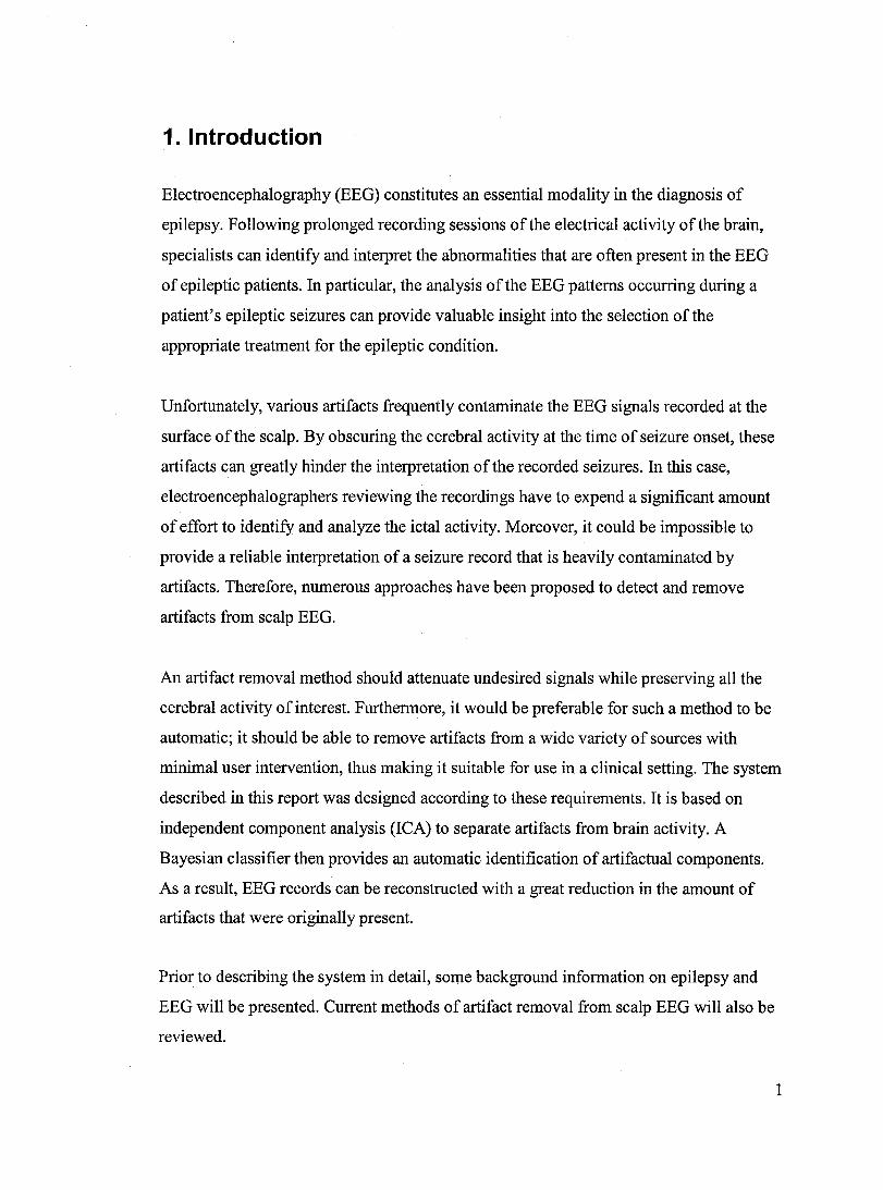
potential along its axon whenever the membrane potential reaches a threshold of
approximately -40m V (Figure 1). An increase in membrane potential (depolarization)
will thus improve the likelihood of firing an action potential. Rence this is referred to as
an excitatory postsynaptic potential (EPSP). On the other hand, an inhibitory postsynaptic
potential (IPSP) is a temporary decrease in membrane potential (hyperpolarization). The
generation of action potentials by the neuron is thus determined by the integration of
EPSPs and IPSPs from synaptic connections with other neurons.
+2ü ~
"" ~ ~.> ;r Si s::::
0
,~ l! ~~ -20 r. 0 ~, t:.. .. 'fi, ~ -40 •• 'Ih:f:whold •• _ • .. l". 0 ••••• _._ ..... "" ........
-60 v_
~ .......... !IlI! .... ~
EPSP Multiple EPSPs IPSP leading ta AP
Time(ms}
Figure 1. EPSPs and IPSPs respectively drive the membrane potential toward or away from the threshold potential. Whenever the combined effect of post-synaptic potentials cause the membrane potential to reach the threshold, an action potential (AP) is generated. Reproduced from (Purves et al.,2001).
Action potentials are caused by the sudden opening of several voltage-controlled Na +
channels whenever the membrane potential threshold is reached, resulting in the complete
depolarization of the cell in less than Ims. Rowever, the resting membrane potential is
quickly restored by facilitated diffusion ofK+ ions out of the cell. After a briefrefractory
period of a few milliseconds, the neuron is able to fire again. An action potential travels
along the axon of the neuron until it reaches the axon terminaIs, which form synaptic
connections with subsequent neurons. An incoming action potential causes the release of
neurotransmitters at the synapse, which again leads to the generation ofEPSPs or IPSPs
in the postsynaptic cells.
5
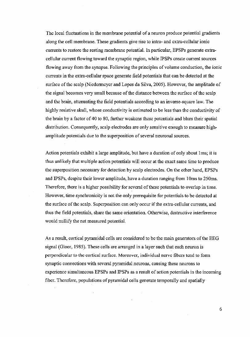
The local fluctuations in the membrane potential of a neuron produce potential gradients
along the cell membrane. These gradients give rise to intra- and extra-cellular ionic
currents to restore the resting membrane potential. In particular, EPSPs generate extra
cellular current flowing toward the synaptic region, while IPSPs create current sources
flowing away from the synapse. Following the principles ofvolume conduction, the ionic
currents in the extra-cellular space generate field potentials that can be detected at the
surface ofthe scalp (Niedermeyer and Lopes da Silva, 2005). However, the amplitude of
the signal becomes very small because of the distance between the surface of the scalp
and the brain, attenuating the field potentials according to an inverse-square law. The
highly resistive skull, whose conductivity is estimated to be less than the conductivity of
the brain by a factor of 40 to 80, further weakens these potentials and blurs their spatial
distribution. Consequently, scalp electrodes are only sensitive enough to measure high
amplitude potentials due to the superposition of several neuronal sources.
Action potentials exhibit a large amplitude, but have a duration of only about Ims; it is
thus unlikely that multiple action potentials will occur at the exact same time to produce
the superposition necessary for detection by scalp electrodes. On the other hand, EPSPs
and IPSPs, despite their lower amplitude, have a duration ranging from 10ms to 250ms.
Therefore, there is a higher possibility for several of these potentials to overlap in time.
However, time synchronicity is not the only prerequisite for potentials to be detected at
the surface of the scalp. Superposition can only occur if the extra-cellular currents, and
thus the field potentials, share the same orientation. Otherwise, destructive interference
would nullify the net measured potential.
As a result, cortical pyramidal cells are considered to be the main generators of the EEG
signal (Gloor, 1985). These cells are arranged in a layer such that each neuron is
perpendicular to the cortical surface. Moreover, individual nerve fibers tend to fonn
synaptic connections with several pyramidal neurons, causing these neurons to
experience simultaneous EPSPs and IPSPs as a result of action potentials in the incoming
fiber. Therefore, populations of pyramidal cells generate temporally and spatially
6
synchronous field potentials whose summation can be measured at the surface of the
scalp.
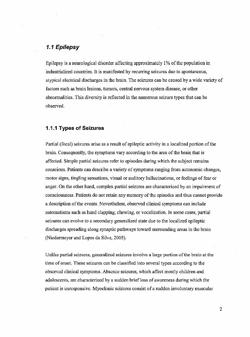
Pyramidal neurons are characterized by a long apical dendritic tree extending from the
soma toward the upper layers of the cortex (Figure 2). Synaptic connections tend to occur
either at basal dendrites near the soma or at distal dendrites extending from the apical
trunk. The generation of current sinks and sources due to EPSPs and IPSPs thus mostly
take place at either end of the apical dendritic trunk. This configuration corresponds to an
electrical dipole (Gloor, 1985). In practice, a single equivalent current dipole is often
used to mode! an entire patch of cortex rather than individual neurons. As mentioned
previously, localized populations of pyramidal cells tend to behave synchronously; they
can often be approximately modelled by a single dipole situated near the centre of the
group of active neurons.
Apical Dendrites
Basal Dendrites
Synaptic Terminais
Figure 2. Structure of a pyramidal neuron. Reproduced from (Farabee, 2001).
7
1.2.2 Scalp EEG
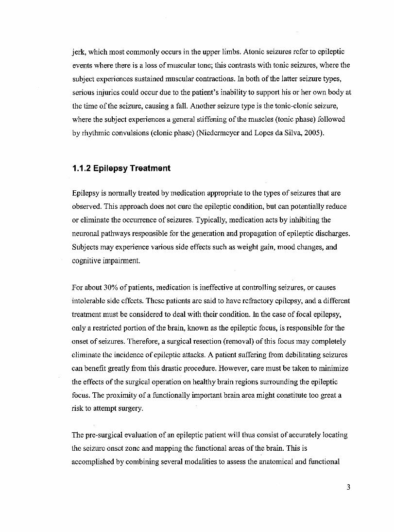
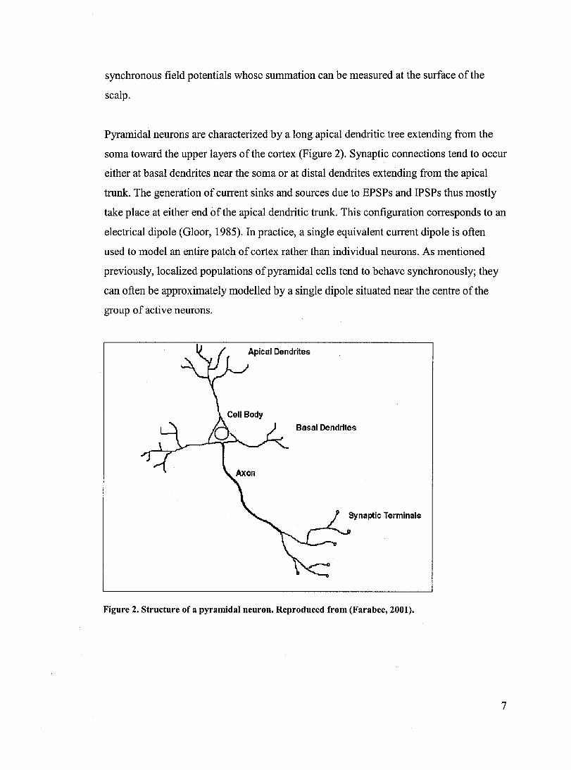
Scalp electrodes are small metal disks that are fixed to the head by a conducting gel that
provides good electrical contact between the electrode and the skin. Electrode placement
is determined by the international 10-20 system of the International Federation of
Societies for Electroencephalography and Clinical Neurophysiology (Jasper, 1958). This
standard establishes the positions and nomenclature of scalp electrodes (Figure 3).
Electrodes are identified by one or two letters corresponding to the cerebral region
underneath them (Fp: frontal pole, F: frontal lobe, C: central region, T: temporal lobe, P:
parietal lobe, 0: occipital lobe ). Within each region, a number marks the position of the
e1ectrode, using odd numbers for the left hemisphere and even numbers for the right
hemisphere. The letter "z" identifies electrodes situated on the midline. Electrodes are
placed at intervals of 10% or 20% of the distance between anatomicallandmarks such as
the nasion, inion, and the left and right preauricular points (hence the name "10-20
system").
Other systems of scalp electrode placement exist to accommodate additional electrodes,
notably the 10-10 system, which exc1usively uses inter-electrode intervals of 10%. The
use of standard electrode positions ensures that a repeatable setup will be used whenever
a patient requires multiple recording sessions. This will also reduce the variability across
patients, although discrepancies will still exist due to differences between head shapes.
Scalp electrodes measure the electrical potentials at the surface of the head, with respect
to a given reference. It is essential to use a reference situated on the head; the use of a
distant reference would cause external potential sources to overwhelm the brain signaIs,
which are of the order of microvolts. However, a good reference should also contain as
little brain activity as possible, which is problematic. Rather than using this referential
montage, another approach is to compute the potential difference between successive
electrodes; this arrangement is referred to as a bipolar montage. It is also possible to use
an average montage, where the average of several electrodes are taken as the common
reference signal.
8
A
Figure 3. The international 10-20 system of electrode placement and nomenclature. Reproduced from (Malmivuo and Plonsey, 1995).
1.2.3 Intracranial EEG
Scalp EEG can only provide a partial representation ofthe electrical activity ofthe brain.
The intensity of the field potentials falls off quickly with distance and is further
attenuated by the skull; scalp electrodes are thus only sensitive to cortical sources situated
close to the surface of the head. To measure activity from deeper structures, intracranial
electrodes need to be surgically positioned directly on the surface ofthe cortex, or even
implanted inside the brain. Again, because of the rapid attenuation of the field potentials
with distance, intracranial electrodes can only measure activity in a small region around
the sensor. Moreover, intracranial recordings clearly constitute an invasive procedure;
electrode implantation is only considered when other non-invasive methods fail to
provide an accurate Iocalization of the epileptic focus. To reduce the risks associated with
the implantation procedure, it is aiso preferable to limit the number of electrodes used to
record the intracranial potentials. It is thus essential that electrodes be positioned at
locations where epileptic foci are likely to be present. Scalp EEG recordings should at
least provide an approximate localization of epileptogenic sources, so that it can guide the
9
positioning of intracranial electrodes, which then serve to further improve the localization
accuracy.
1.2.4 EEG Patterns
The localization of seizure onset zones using scalp EEG first requires trained
electroencephalographers to distinguish epileptiform EEG patterns from normal activity.
EEG signaIs are usually characterized by their energy in the frequency bands shown in
table 1 (Niedermeyer and Lopes da Silva, 2005).
EEG band Frequencies
Delta 0.1-3.5 Hz
Theta 4-7.5 Hz
Alpha 8-13 Hz
Beta 14-40 Hz
Table 1. Definition of the frequency bands used to describe EEG activity.
In a normal healthy adult, the EEG characteristics depend mainly on the state of alertness
of the subj ect. Beta activity is usually associated with a state of alert wakefulness,
whereas the alpha rhythm occurs when the subject, while still awake, enters a relaxed
state, notably by c10sing his or her eyes. A drop in the alpha rhythm in conjunction with
the appearance oftheta activity marks the onset of sleep. Finally, large-amplitude delta
waves characterize stages of deep sleep.
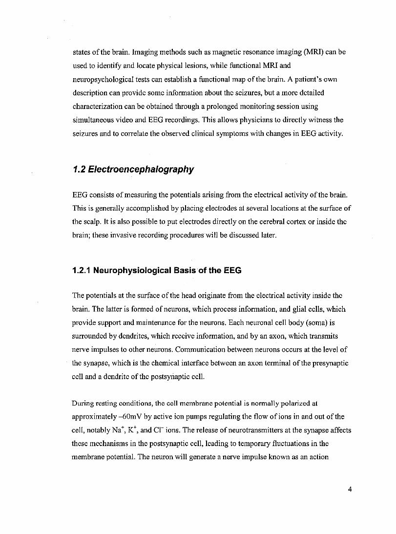
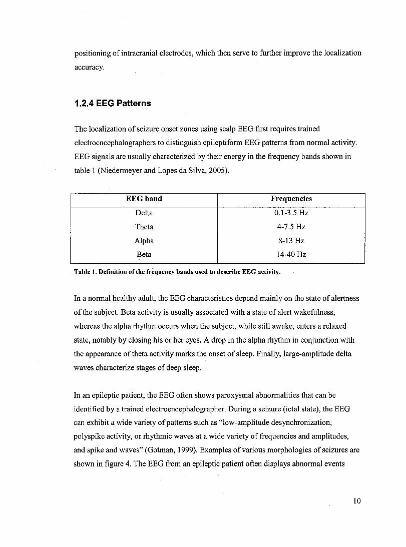
In an epileptic patient, the EEG often shows paroxysmal abnormalities that can be
identified by a trained electroencephalographer. During a seizure (ictal state), the EEG
can exhibit a wide variety of patterns such as "low-amplitude desynchronization,
polyspike activity, or rhythmic waves at a wide variety of frequencies and amplitudes,
and spike and waves" (Gotman, 1999). Examples ofvarious morphologies ofseizures are
shown in figure 4. The EEG from an epileptic patient often displays abnormal events
10
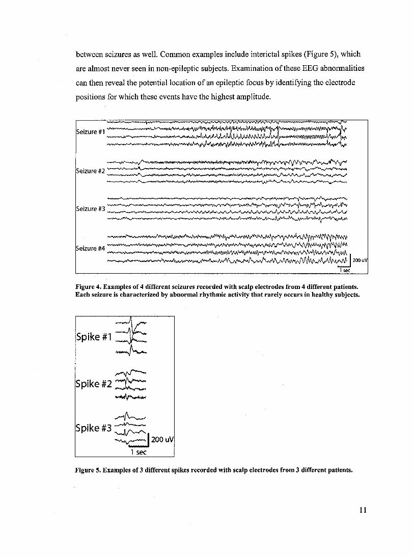
between seizures as weIl. Cornrnon examples inc1ude interictal spikes (Figure 5), which
are alrnost never seen in non-epileptic subjects. Exarnination ofthese EEG abnormalities
can then reveal the potentiallocation of an epileptic focus by identifying the electrode
positions for which these events have the highest amplitude.
Figure 4. Examples of 4 different seizures recorded with scalp electrodes from 4 different patients. Each seizure is characterized by abnormal rhythmic activity that rarely occurs in healthy subjects.
Spike #1
~ Spike #2 ::J::;::; ~
~ Spike#3~
~1200UV 1 sec
Figure 5. Examples of 3 different spikes recorded with scalp electrodes from 3 different patients.
11
1.2.5 EEG Artifacts
Multiple sources of artifacts can contaminate the EEG recorded by scalp electrodes.
These artifacts often complicate the interpretation of the EEG by obscuring the cerebral
activity of interest.
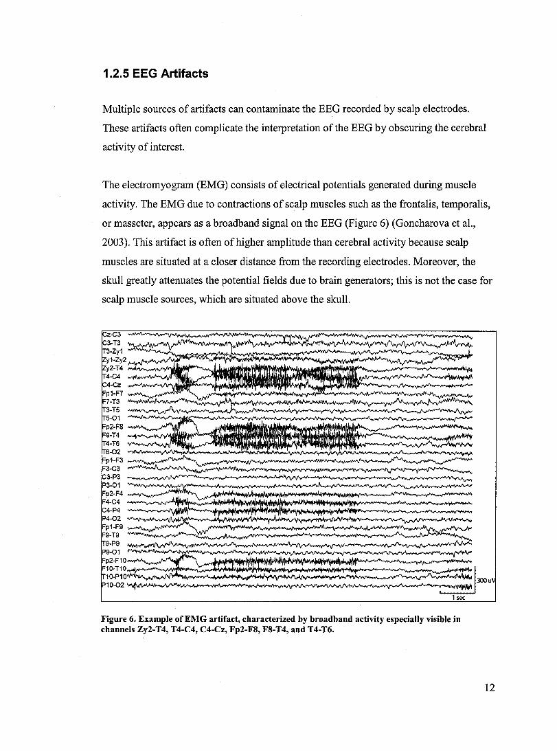
The electromyogram (EMG) consists of electrical potentials generated during muscle
activity. The EMG due to contractions of scalp muscles such as the frontalis, temporalis,
or masseter, appears as a broadband signal on the EEG (Figure 6) (Goncharova et al.,
2003). This artifact is often ofhigher amplitude than cerebral activity because scalp
muscles are situated at a closer distance from the recording electrodes. Moreover, the
skull greatly attenuates the potential fields due to brain generators; this is not the case for
scalp muscle sources, which are situated above the skull.
Figure 6. Example of EMG artifact, characterized by broadband activity especially visible in channels Zy2-T4, T4-C4, C4-Cz, Fp2-F8, F8-T4, and T4-T6.
12
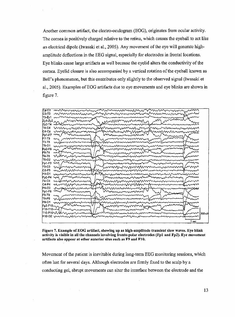
Another common artifact, the electro-oculogram (EOG), originates from ocular activity.
The comea is positively charged relative to the retina, which causes the eyeball to act like
an electrical dipole (Iwasaki et al., 2005). Any movement of the eye will generate high
amplitude deflections in the EEG signal, especially for electrodes in frontal locations.
Eye blinks cause large artifacts as weIl because the eyelid alters the conductivity of the
comea. Eyelid closure is also accompanied by a vertical rotation ofthe eyeball known as
BeIl's phenomenon, but this contributes only slightly to the observed signal (Iwasaki et
al., 2005). Examples of EOG artifacts due to eye movements and eye blinks are shown in
figure 7.
Figure 7. Example of EOG artifact, showing up as high-amplitude transient slow waves. Eye blink activity is visible in ail the channels involving fronto-polar electrodes (Fpl and Fp2). Eye movement artifacts also appear at other anterior sites such as F9 and FIO.
Movement of the patient is inevitable during long-term EEG monitoring sessions, which
often last for several days. Although electrodes are firmly fixed to the scalp by a
conducting gel, abrupt movements can alter the interface between the electrode and the
13
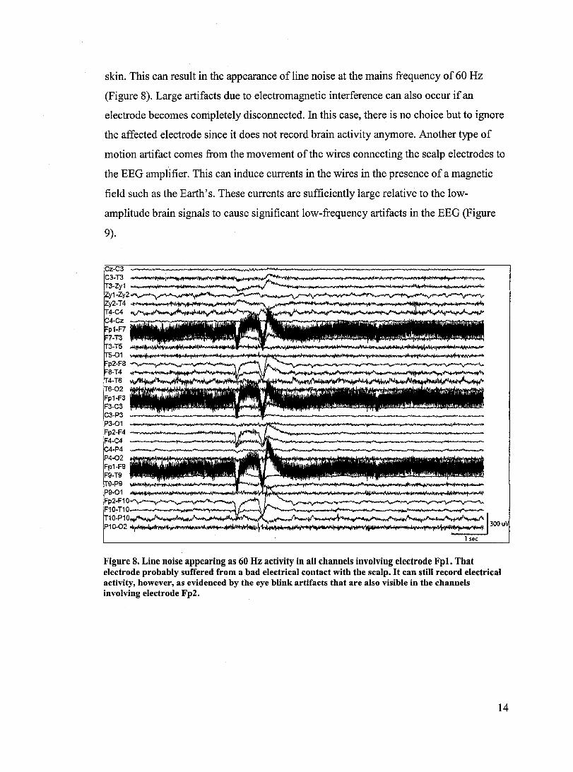
skin. This can result in the appearance of line noise at the mains frequency of 60 Hz
(Figure 8). Large artifacts due to electromagnetic interference can also occur if an
e1ectrode becomes completely disconnected. In this case, there is no choice but to ignore
the affected electrode since it does not record brain activity anymore. Another type of
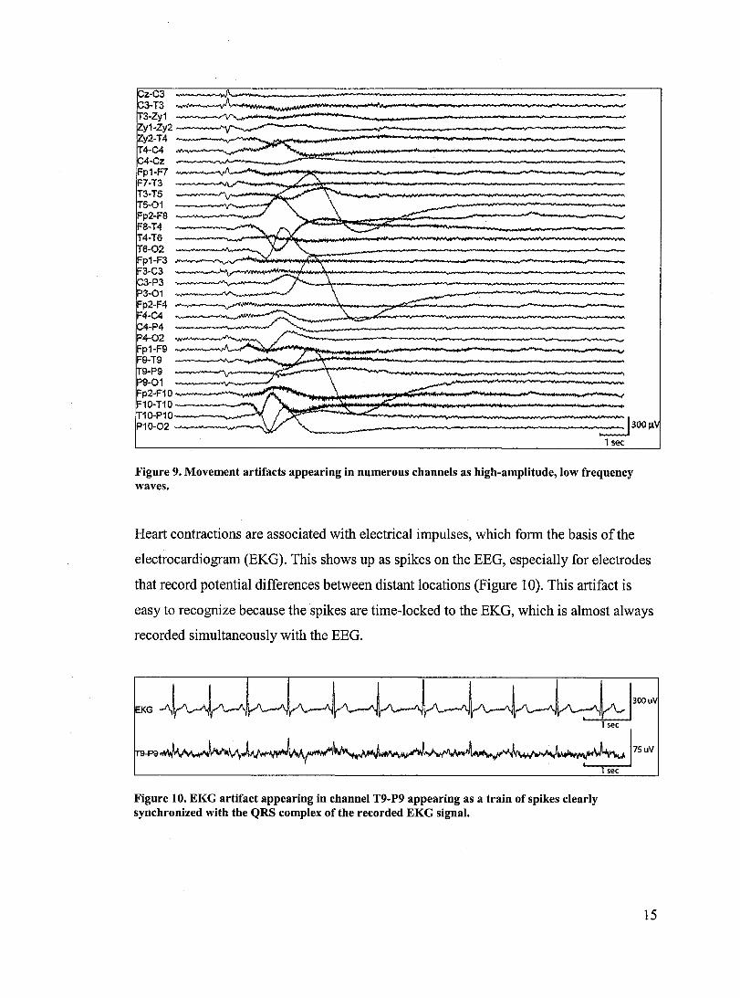
motion artifact cornes from the movement ofthe wires connecting the scalp electrodes to
the EEG amplifier. This can induce currents in the wires in the presence of a magnetic
field such as the Earth's. These currents are sufficiently large relative to the low
amplitude brain signaIs to cause significant low-frequency artifacts in the EEG (Figure
9).
Figure 8. Line noise appearing as 60 Hz activity in ail channels involving electrode Fpl. That electrode probably suffered from a bad electrical contact with the scalp. If can still record electrical activity, however, as evidenced by the eye blink artifacts that are also visible in the channels involving electrode Fp2.
14
_._ ....... _ .......... 't ....... _____ ~"""" .... __ ioifO'~_,...,_ .. _~
.. "" ....
------------,~~:::_::-:=~.-.----:===
~ ____ ------~~------------~-------~300~ 1 sec
Figure 9. Movement artifacts appearing in numerous channels as high-amplitude, low frequency waves.
Heart contractions are associated with electrical impulses, which form the basis of the
electrocardiogram (EKG). This shows up as spikes on the EEG, especially for electrodes
that record potential differences between distant locations (Figure 10). This artifact is
easy to recognize because the spikes are time-Iocked to the EKG, which is almost always
recorded simultaneously with the EEG.
Figure 10. EKG artifact appearing in channel T9-P9 appearing as a train of spikes c1early synchronized with the QRS complex of the recorded EKG signal.
15
1.3 Artifact Removal from the EEG
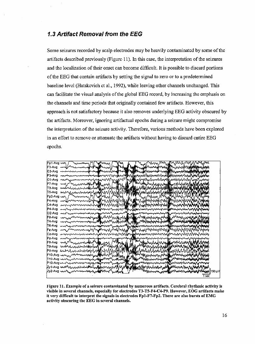
Sorne seizures recorded by scalp electrodes may be heavily contaminated by sorne of the
artifacts described previously (Figure Il). In this case, the interpretation of the seizures
and the localization oftheir onset can become difficult. It is possible to discard portions
of the EEG that contain artifacts by setting the signal to zero or to a predetermined
baseline level (Hatskevich et al., 1992), while leaving other channels unchanged. This
can facilitate the visual analysis of the global EEG record, by increasing the emphasis on
the channels and time periods that originally contained few artifacts. However, this
approach is not satisfactory because it also removes underlying EEG activity obscured by
the artifacts. Moreover, ignoring artifactual epochs during a seizure might compromise
the interpretation ofthe seizure activity. Therefore, various methods have been explored
in an effort to remove or attenuate the artifacts without having to discard entire EEG
epochs.
Figure 11. Exarnple of a seizure contaminated by nurnerous artifacts. Cerebral rhythrnic activity is visible in several channels, especially for electrodes T3-T5-F4-C4-P9. However, EOG artifacts rnake it very difficuIt to interpret the signais in electrodes Fpl-F7-Fp2. There are also bursts ofEMG activity obscuring the EEG in several channels.
16
1.3.1 EOG Regression Methods
The EOG signal can be measured by periocular electrodes and subsequently subtracted
from the recorded EEG. The potentials due to ocular activity propagate to the scalp
electrodes by volume conduction; each electrode site will thus be affected differently,
particularly as a function of their distance from the eyes. Since the EOG artifact tends to
be of much larger amplitude than brain signaIs, it is possible to estimate the contribution
of the oeular aetivity at eaeh eleetrode by regression methods (Gratton et al., 1983). The
EOG, appropriately scaled for each electrode site, can then be subtracted from the EEG
signal. Another approach consists of performing the regression and subtraction ofthe
EOG in the frequency domain (Whitton et al., 1978). In this case, the regression scaling
factors are determined by comparing the spectra of the EOG and the EEG, particularly
for the low frequencies that predominate in the EOG.
EOG subtraction methods rely on the assumption that the regression scaling factors at
each electrode position would be the same for both eye movements and eye blinks.
However, the eye movement artifact is caused by the ocular dipole, while the eye blink
artifact is mainly due to the properties of the eyelid (Iwasaki et al., 2005). These two
types of artifacts are thus caused by distinct mechanisms that propagate differently to the
scalp. The amplitude of eye blink artifacts decreases rapidly with distance from the eyes,
while eye movement artifacts can significantly affect even distant electrode locations
(Gasser et al., 1985). Consequently, it is not possible to determine a scaling factor for the
EOG that will completely remove both types of ocular artifacts from the EEG.
Another limitation ofthis approach cornes from the fact that electrical signaIs due to
brain activity propagate everywhere at the surface ofthe head, inc1uding at EOO
recording sites. The EOG electrodes do not measure pure ocular activity, but rather a
mixture of ocular and cerebral activity. Subtraction of the EOG signal will thus attenuate
relevant brain signaIs in the EEG, and might even introduce extraneous neural activity at
sorne electrode sites (Jung et al., 2000a). Regression methods thus fail to produce
17
adequate artifact elimination due to the inability to measure artifactual sources directly,
without contamination from brain signaIs.
1.3.2 Digital Filtering
Frequency-domain filtering has also been explored as a method to remove artifacts from
EEG records. In particular, cerebral seizure activity mostly occurs at frequencies below
30 Hz, while scalp muscle artifacts have a broader spectrum (Gotman et al., 1981).
Filtering out any activity above 30 Hz can eliminate a sizable portion of the EMG artifact
with only a minimal effect on the underlying cerebral activity. However, it has been
shown that the EMG also contains significant power at frequencies below 30 Hz
(O'Donnell et al., 1974). Even after a low-pass filtering operation, the EEG would thus
still be contaminated by EMG activity, especially for scalp electrodes positioned near the
contracting muscles.
Similarly, a high-pass filter could be used to partially eliminate low-frequency movement
artifacts from the EEG. Yet again, the overlap between the frequency spectra of the
cerebral activity and the artifacts prevent a complete removal of the artifactual signaIs.
Therefore, frequency-domain methods fail to adequately separate artifacts from EEG
recordings.
1.3.3 Principal Component Analysis
The EEG is recorded with multiple electrodes simultaneously, hence generating a multi
dimensional dataset. The method of principal component analysis (PCA) consists of
expressing this dataset as a linear combination of several uncorrelated components. This
is accomplished by removing the mean from the data and performing a singular value
decomposition (SVD) of the covariance matrix of the EEG record, for which the resulting
eigenvectors form an orthogonal basis. After arranging the eigenvectors in decreasing
order oftheir corresponding eigenvalues, the centered dataset is projected along these
eigenvectors to form an ordered set known as the principal components of the data. It can
18
be shown that the first principal component corresponds to the projection ofthe data of
maximal variance. Moreover, subsequent principal components are also ofmaximal
variance under the constraint that they be uncorrelated with all previous components
(Hyvarinen et al., 2001).
In many cases of applying PCA to EEG recordings, it has been found that sorne
artifactual activity was isolated exc1usively in a few components (Lagerlund et al., 1997).
It would be possible to reconstruct the EEG dataset using only the non-artifactual
components, hence using PCA as a kind spatial filter to remove the identified artifacts.
Since artifacts and cerebral activity are generated by different mechanisms, the
uncorrelatedness constraint supports the generation of components that separate
artifactual activity from brain signaIs.
In PCA, the eigenvectors corresponding to the directions of the principal components are
restricted to be orthogonal. Applied to EEG recordings, these eigenvectors represent
spatial maps indicating the contributions of each component to each electrode position.
However, there are many cases where the topography of a brain signal is not orthogonal
to that of an artifact. For example, seizure activity originating in the frontal lobe and
ocular activity can have very similar spatial maps. As a result, PCA will fail to separate
these two sources into distinct components (Ille et al., 2002).
Nevertheless, PCA can still successfully extract artifacts from EEG records iftheir
amplitude is much larger than the relevant brain signaIs. In particular, the first principal
component corresponds exactly to the direction of maximal variance of the data and is
not subject to an orthogonality constraint. However, the remaining components are
unlikely to represent individual sources, and lower-amplitude artifacts thus cannot be
removed using this method.
19
1.3.4 Independent Component Analysis
The representation of a dataset as a linear combination ofuncorrelated sources is an ill
defined problem with an infinite number of solutions. It is for this reason that PCA
imposes additional constraints of variance maximization and orthogonality ofprojection
directions, hence generating a unique set of components. However, as has been noted
above, the orthogonality constraint is not applicable to EEG sources, and PCA thus fails
to adequately separate artifacts from brain activity.
In recent years, the method of independent component analysis (ICA) has been deve10ped
to perform blind source separation. ICA constrains the extracted sources to be statistically
independent, which is a stronger assumption than the uncorrelatedness required by PCA.
While uncorrelated signaIs are merely required to have no linear relationship,
independent signaIs cannot be related by non-linear functions as weIl. Since cerebral
activity and artifacts originate from different mechanisms, the electrical signaIs
manifested by these sources are indeed expected to be statistically independent. ICA then
models the signal measured at each electrode as a linear mixture of the sources:
A=WX (1)
In the above equation, X represents the time courses of each independent source and W is
a linear mixing matrix indicating the contribution of the sources to each electrode. The
matrix A contains the time courses of each mixture. ICA then consists of estimating the
matrices W and X, given only the mixtures A. This is a technique ofblind source
separation, meaning that no assumptions are made on the morphologies ofthe sources X
The ICA mode1 does not incorporate a noise term, since any source of noise can be
considered as one of the independent sources in X.
It should be noted that the model assumes that the sources are mixed linearly and
instantaneously at each electrode site. This is a reasonable assumption for EEG signaIs,
which propagate by volume conduction. The quasi-static approximation ofMaxwell's
20
equations, which has been shown to be valid for the conductivities found in biological
tissues and for frequencies under 1 kHz (Malmivuo and Plonsey, 1995), implies that EEG
signaIs reach the scalp with negligible propagation delays. The ICA model is thus an
appropriate representation of the activity recorded at each electrode.
ICA uses high-order statistics to extract a set of independent components. This set is
unique, up to scaling and permutation, as long as at most one of the sources is Gaussian
(Hyvarinen et al., 2001). This is because whenever two Gaussian signaIs are uncorrelated,
they are also guaranteed to be independent. Higher-order cross-correlations of
uncorrelated Gaussian signaIs are equal to zero; in this case, independence is thus
equivalent to uncorrelatedness. The higher-order statistics thus do not provide additional
information that will allow ICA to extract the original sources. Consequently, ICA cannot
separate a mixture ofindependent sources ifmore than one is Gaussian. Nevertheless,
scalp electrodes record synchronous brain activity that consists ofvarious rhythms with a
non-Gaussian distribution. Moreover, many sources of artifacts consist ofhigh-amplitude
transients and thus are super-Gaussian, meaning that their distribution has heavier tails
than a Gaussian distribution. These non-Gaussian distributions allow ICA to successfully
separate cerebral activity and artifacts into distinct components.
A final requirement of ICA is that the number of mixtures should be equal to the number
of original sources. However, this is rarely the case in EEG analysis, since the number of
brain sources is unknown beforehand, while the number of electrodes is fixed. If the
number of sources is less than the number of mixtures, this is referred to as the under
complete case. This situation can be detected by performing PCA as a pre-processing step
to reduce the dimensionality ofthe data. The SVD performed in PCA will yield
eigenvalues that are equal to zero, corresponding to dimensions that can be eliminated
without any 10ss of information. However, the numerous sources of artifacts and noise
present at each electrode ensure that the under-complete case is unlikely to happen when
performing ICA on EEG signaIs. On the other hand, the over-complete case occurs when
the number of sources is greater than the number of electrodes. As a result, ICA will be
unable to extract aIl of the original sources. Nevertheless, it has been shown that ICA is
21
sufficiently robust to extract the highest amplitude sources into separate components,
while the weaker sources become distributed among components with similar spatial
distributions (Makeig et al., 1996a).
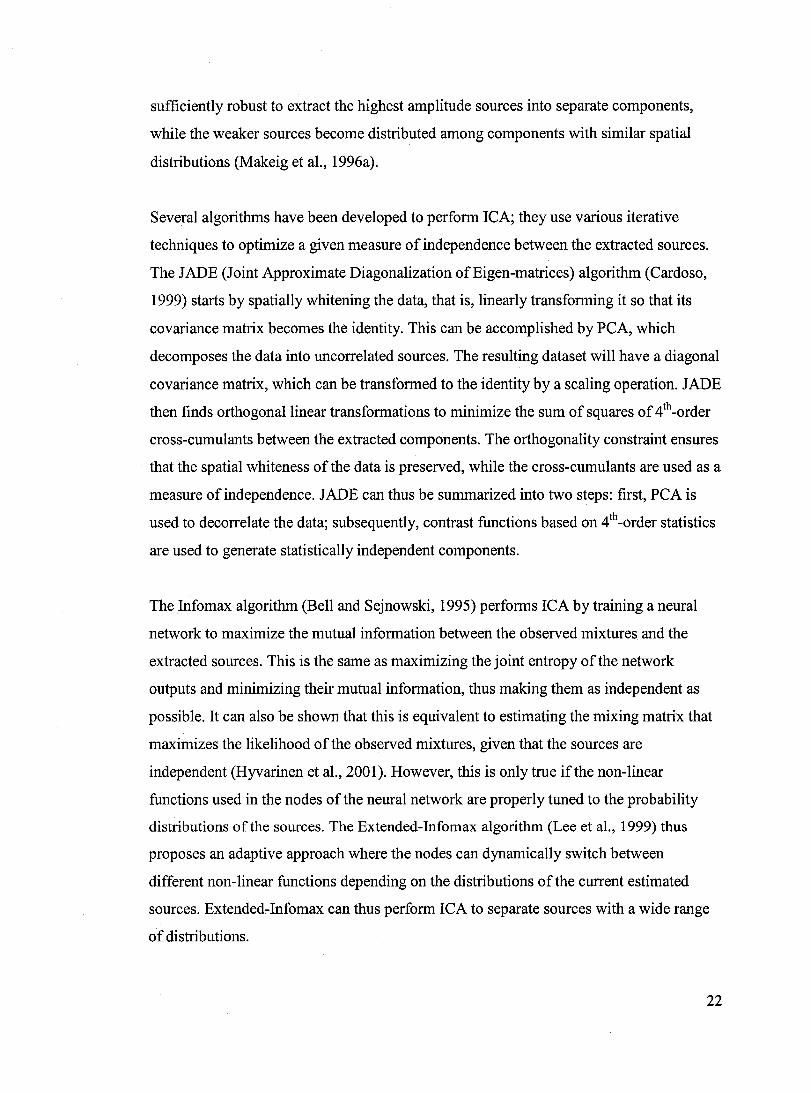
Several algorithms have been developed to perform ICA; they use various iterative
techniques to optimize a given measure of independence between the extracted sources.
The JADE (Joint Approximate Diagonalization of Eigen-matrices) algorithm (Cardoso,
1999) starts by spatially whitening the data, that is, linearly transforming it so that its
covariance matrix becomes the identity. This can be accomplished by PCA, which
decomposes the data into uncorrelated sources. The resulting dataset will have a diagonal
covariance matrix, which can be transformed to the identity by a scaling operation. JADE
then finds orthogonallinear transformations to minimize the sum of squares of 4th -order
cross-cumulants between the extracted components. The orthogonality constraint ensures
that the spatial whiteness of the data is preserved, while the cross-cumulants are used as a
measure ofindependence. JADE can thus be summarized into two steps: first, PCA is
used to decorrelate the data; subsequently, contrast functions based on 4th -order statistics
are used to generate statistically independent components.
The Infomax algorithm (Bell and Sejnowski, 1995) performs ICA by training a neural
network to maximize the mutual information between the observed mixtures and the
extracted sources. This is the same as maximizing the joint entropy ofthe network
outputs and minimizing their mutual information, thus making them as independent as
possible. It can also be shown that this is equivalent to estimating the mixing matrix that
maximizes the likelihood of the observed mixtures, given that the sources are
independent (Hyvarinen et al., 2001). However, this is only true ifthe non-linear
functions used in the nodes of the neural network are properly tuned to the probability
distributions of the sources. The Extended-Infomax algorithm (Lee et al., 1999) thus
proposes an adaptive approach where the nodes can dynamically switch between
different non-linear functions depending on the distributions ofthe current estimated
sources. Extended-Infomax can thus perform ICA to separate sources with a wide range
of distributions.
22

FastICA (Hyvarinen and Oja, 2000) is another popular algorithm that, similar to JADE,
uses PCA as a pre-processing step to generate spatially whitened data. It then uses a
fixed-point method to find an orthogonal transformation that maximizes the negentropy
of the extracted sources. The negentropy is the difference between the entropy of a signal
and that of a Gaussian variable with the same variance. It can be shown that, given a
fixed variance, the entropy is maximal for Gaussian distributions. The negentropy is thus
used as a measure ofnon-Gaussianity of the signaIs. In a linear mixture ofindependent
sources, the centrallimit theorem implies that the distribution of the mixture will become
c10ser to Gaussian than the original signaIs. Maximizing the non-Gaussianity of the
extracted signaIs will thus tend to separate the original sources.
In practice, the entropy calculations are computationally expensive. Therefore, FastICA
uses the following robust approximation (Hyvarinen and Oja, 2000):
J(y) oc [E{G(y)} -E{G(U)}]2 (2)
where J(y) is the negentropy of the variable y, standardized to have zero mean and unit
variance, E {.} denotes the expected value, f-l is a Gaussian random variable of zero mean
and unit variance, and G(.) is the contrast function log(cosh(.)).
The fixed-point iterative method used to maximize this measure ensures that FastICA
converges rapidly to the ICA results. FastICA thus tends to offer a better computational
performance than JADE or Extended-Infomax. Aside from this issue ofspeed, aIl ofthe
algorithms described above will tend to yield similar results, since ICA has a unique
solution as long as the various assumptions described previously are met.
ICA can be an effective tool to separate strong artifacts from cerebral activity in EEG
signaIs. In particular, seizure recordings can become easier to interpret by c1inicians after
performing artifact removal using ICA (Urrestarazu et al., 2004). Using any ofthe
algorithms outlined above, trained electroencephalographers can visually inspect the
23
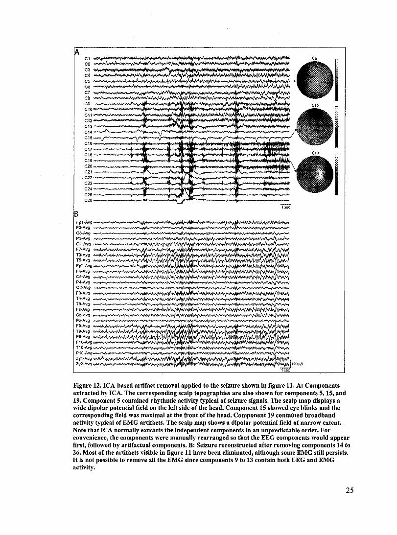
components extracted by ICA and remove those corresponding to artifactual sources
(Figure 12). The seizure record can then be reconstructed using the remaining
components. Since artifacts were removed, the area and time of onset of seizures become
easier to identify, cerebral activity becomes clearer, and the diagnosis value of the EEG
improves. It has also been demonstrated that this improvement in the interpretability of
the EEG is superior to that obtained by digital filters alone (Urrestarazu et al., 2004).
However, this methodology is impractical for clinical use because the visual inspection
and manual selection of artifactual components is too tedious (Jung et al., 2000b). The
application of ICA generates a large number of components, equal to the number of
electrodes. While sorne components can be quickly recognized as either brain activity or
artifacts, there are many cases where this task requires a careful examination of a
component's time course and spatial topography.
1.3.5 Automatic Artifact Removal using ICA
The aim of this work was thus to develop a system that could automatically classify the
components generated by ICA from seizure records. The artifact removal would then be
performed instantaneously, without requiring any human intervention. A few systems
have already been devised to identify sorne of the features that characterize artifactual
components (Delorme et al., 2001; Barbati et al., 2004). However, these semi-automatic
systems still require a trained electroencephalographer to review the computed features
and decide whether to retain or remove each component.
24
Cl C2 C3 C4 C5 C6 C7 CS C9 C10 C11 C12 C13 C14 C15 C16 C17 C18 C19 C20 C21
" C22 C23 C24 C25 C26
"i'5eë B
~
Figure 12. ICA-based artifact removal applied to the seizure shown in figure 11. A: Components extracted by ICA. The corresponding scalp topographies are also shown for components 5, 15, and 19. Component 5 contained rhythmic activity typical of seizure signais. The scalp map displays a wide dipolar potential field on the left side of the head. Component 15 showed eye blinks and the corresponding field was maximal at the front of the head. Component 19 contained broadband activity typical of EMG artifacts. The scalp map shows a dipolar potential field of narrow extent. Note that ICA normally extracts the independent components in an unpredictable order. For convenience, the components were manually rearranged so that the EEG components would appear first, followed by artifactual components. B: Seizure reconstructed after removing components 14 to 26. Most of the artifacts visible in figure 11 have been eliminated, although sorne EMG still persists. It is not possible to remove ail the EMG since components 9 to 13 contain both EEG and EMG activity.
25
Another approach consists of selecting components highly correlated with a reference
signal such as the EOG (Park et al., 2003). Recently, constrained-ICA algorithms have
also been developed to specifically extract individual components highly correlated with
a given reference (James and Gibson, 2003; Lu and Rajapakse, 2005). These methods can
be very effective to remove particular artifacts for which a reference signal can be
measured. However, an EOG is not always recorded simultaneously with the EEG. AIso,
many other types of artifactual sources cannot be measured separately to serve as a
reference. For example, the EMG signal is the result ofthe summation of the activity
from thousands of asynchronous muscle cells. The signal will thus vary greatly
depending on where it is measured along the muscle, so there is no unique reference that
can be used. In that case, automatic methods must re1y on extracting features to recognize
artifactual components. A lot of research has focused on the automatic recognition of
ocular artifacts extracted by ICA using a combination of spectral features, spatial
topography, and time-domain signal morphology (Delsanto et al., 2003; Romero et al.,
2004). However, these approaehes are specifie to oeular artifacts and eannot be easily
extended to other unwanted signaIs.
The system described in this report can perform the artifact removal automatically and is
thus well suited for clinical purposes. Moreover, rather than being specifically tuned to
particular artifacts, the system can simultaneously remove several different types of
artifacts.
26
2. Methods
2. 1 Data Selection
Scalp EEG recordings of 205 seizures from 46 epileptic patients were collected at the
Montreal Neurological Institute using the Stellate Harmonie system (Stellate, Montreal,
Quebec, Canada), between December 2000 and February 2004. Patients were only
selected if at least two seizures were recorded on the EEG. There was no pre-selection
with respect to the amount of artifacts that were present. The seizures did not have to be
accompanied by clinical symptoms, but they all had to show visible changes on the EEG
signal. The resulting dataset included a wide variety of seizures; 35 patients had focal
seizures, while Il patients suffered from generalized epilepsy. Each patient had between
21 and 39 scalp electrodes with a common reference at FCz. The recorded signaIs were
sampled at 200Hz after filtering between 0.5 and 70Hz and were then re-referenced into
an average montage. The choice of the montage does not influence the results ofICA,
since it only changes the linear mixtures of the signal sources without affecting the
sources themse1ves. The rationale behind the selection of a referential montage was that it
allows the generation of topographie maps of the scalp potentials.
2.2 Artifact separation using Independent Component Analysis
Locating the onset of seizures on EEG records is crucial to the evaluation of the epileptic
condition. However, this is not always a straightforward task, especially if artifacts are
present. For each seizure, a 30-second window was selected starting approximately 10
seconds before the time of the visually identified seizure onset. This ensured that the
analyzed segment included a good portion ofthe seizure as well as any early activity that
might not have been identified by visual inspection. Restricting the window length to 30
seconds limited the number of distinct transient artifactual sources that could be present
in the data segment. The FastICA algorithm (Hyvarinen and Oja, 1997) was applied to
these seizure segments, using the EEGLAB platform (Delorme and Makeig, 2004)
27
running on MATLAB (The Mathworks, Natick, Massachusetts). The use of other ICA
algorithms such as Extended Infomax (Lee et al., 1999) yielded similar source separation
results, but FastICA was chosen because its fixed-point method produced faster
convergence. The algorithm extracted statistically independent components whose linear
mixture could be used to reconstruct the original EEG signal. The number of extracted
components was equal to the number of recording electrodes. Each 30-second component
was then partitioned into fifteen 2-second epochs. This partitioning was necessary
because sorne components contained both EEG and artifactual segments, as will be
explained further below. Using visual inspection ofboth the time-domain signal and the
spatial topography associated with each component, the epochs were classified as
representing either EEG or artifactual activity. The small duration of each epoch ensured
that this visual classification was generally unambiguous.
Ocular artifacts were easily identified due to the characteristic low-frequency waveforms
caused by either eye blinks or eye saccades (lwasaki et al., 2005). Moreover, the
consistent spatial topographies of these artifacts provided another distinguishing factor:
eye blinks and vertical eye movements mostly affected fronto-polar electrodes, while
horizontal eye movement artifacts were especially present in the F7-F9-F8-FI0
electrodes, with a phase reversaI between the right and left sides. Patient movement
artifacts were characterized by high-amplitude slow waves; these occurred frequently
when the patients were changing positions during clinical seizures. Electrode artifacts,
due to defective electrodes or faulty connections, could also be clearly identified; they
affected only a single electrode and were characterized by either an unusually high
amplitude signal or significant power at the mains frequency of 60Hz. Another very
common artifact was caused by the EMG (electromyogram) signal from scalp muscle
contractions being recorded by the EEG electrodes. This artifact significantly affects the
EEG due to its broad spectrum showing energy at all frequencies from 0 to 200Hz
(Goncharova et al., 2003). In particular, the EMG spectrum overlaps with the ictal EEG,
whose energy is mainly contained in the frequencies between 3 and 29Hz (Gotman et al.,
1981). Epochs contaminated by EMG could be distinguished from EEG epochs by the
significant high-frequency activity above 30Hz. Moreover, since the EMG sources are
28
situated just below the scalp, they do not suffer from the spatial smearing of EEG sources
due to their distance from the recording surface and the volume conduction through the
highly resistive skuIl, which acts as a lowpass spatial filter (Srinivasan et al., 1998).
Therefore, EMG epochs extracted by ICA were characterized by a very limited spatial
extent. FinaIly, electrocardiogram (EKG) artifacts were also identified as regular spikes
time-Iocked to a reference EKG signal.
ICA-based methods ofEEG artifact removal rely on the elimination or preservation of
components extracted by the algorithm. However, sorne components contained artifactual
transients affecting sorne parts of the signal, while the rest of the time course represented
mainly cerebral activity. To train an automated system to recognize artifacts, it was thus
necessary to partition the 30-second components into smaller 2-second epochs that could
be classified without ambiguity. After manually labelling these epochs as either EEG or
artifact, the entire components themselves were also marked to be either rejected or
preserved. Whenever a component was composed entirely of EEG epochs or artifactual
epochs, it was clear that the component should be kept or removed, respectively. On the
other hand, in the case of a mixture ofboth types of epochs, components were rejected
only if this would result in no significant EEG activity being removed from the seizure
record. In particular, the EEG activity related to the seizure should not be affected by the
rejection of a component. This assessment was based on the reviewer's subjective
judgment, by comparing the original seizure record with the EEG reconstructed from the
component being examined. In the end, not every artifactual activity could be removed
from the recording, since this would have resulted in the loss of EEG activity as weIl.
2.3 Training of an automated artifact rejection system
Figure 13 shows the various stages involved in the training and operation of the
automated artifact rejection system. Briefly, various spectral, statistical, and spatial
features are calculated from the 2-second epochs from each component extracted by ICA.
The continuous features are then discretized by using cutoff thresholds determined from
the training data. The training dataset is also used to induce a Bayesian network to encode
29
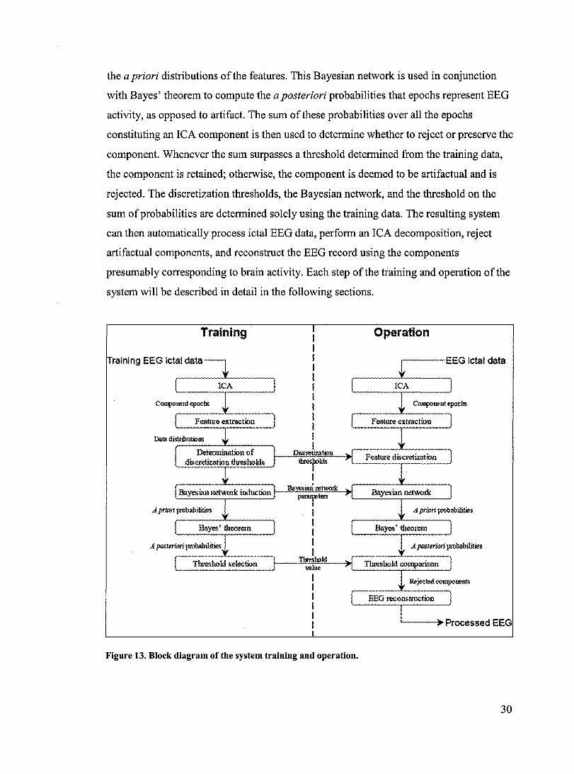
the a priori distributions of the features. This Bayesian network is used in conjunction
with Bayes' theorem to compute the a posteriori probabilities that epochs represent EEG
activity, as opposed to artifact. The sum of these probabilities over all the epochs
constituting an ICA component is then used to determine whether to reject or preserve the
component. Whenever the sum surpasses a threshold determined from the training data,
the component is retained; otherwise, the component is deemed to be artifactual and is
rejected. The discretization thresholds, the Bayesian network, and the threshold on the
sum of probabilities are determined solely using the training data. The resulting system
can then automatically process ictal EEG data, perform an ICA decomposition, reject
artifactual components, and reconstruct the EEG record using the components
presumably corresponding to brain activity. Each step ofthe training and operation of the
system will be described in detail in the following sections.
Training
raining EEG ietal data
1 1 1 1 1 1 1 1 1 1 1 l.
.. parafters
1 1 1 1 1
Thresbold w1ue
1 1 1 1 1 1
n
Figure 13. Block diagram of the system training and operation.
Operation
.----EEG ietal data
'-----è ... Proeessed EEG
30
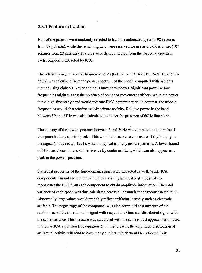
2.3.1 Feature extraction
Half of the patients were randomly selected to train the automated system (98 seizures
from 23 patients), while the remaining data were reserved for use as a validation set (107
seizures from 23 patients). Features were then computed from the 2-second epochs in
each component extracted by ICA.
The relative power in several frequency bands (O-IHz, 1-3Hz, 3-15Hz, 15-30Hz, and 30-
55Hz) was calculated from the power spectrum of the epoch, computed with Welch's
method using eight 50%-overlapping Hamming windows. Significant power at low
frequencies might suggest the presence of ocular or movement artifacts, while the power
in the high-frequency band would indicate EMG contamination. In contrast, the middle
frequencies would characterize mainly seizure activity. Relative power in the band
between 59 and 61Hz was also calculated to detect the presence of 60Hz line noise.
The entropy ofthe power spectrum between 5 and 30Hz was computed to determine if
the epoch had any spectral peaks. This would thus serve as a measure of rhythmicity in
the signal (lnouye et al., 1991), which is typical ofmany seizure patterns. A lower bound
of 5Hz was chosen to avoid interference by ocular artifacts, which can also appear as a
peak in the power spectrum.
Statistical properties of the time-domain signal were extracted as weIl. While ICA
components can only be determined up to a scaling factor, it is still possible to
reconstruct the EEG from each component to obtain amplitude information. The total
variance of each epoch was thus calculated across aIl channels in the reconstructed EEG.
AbnormaIly large values would probably reflect artifactual activity such as electrode
artifacts. The negentropy of the component was aiso computed as a measure of the
randomness of the time-domain signal with respect to a Gaussian-distributed signal with
the same variance. This measure was calculated with the same robust approximation used
in the FastlCA algorithm (see equation 2). In many cases, the amplitude distribution of
artifactual activity will tend to have many outliers, which would be reflected in its
31

negentropy. This property was ca1culated for the entire component, rather than individual
epochs, to ensure that enough data points were used to get an accurate estimate of the
amplitude distribution of the signal.
ICA components were also characterized by a spatial topography corresponding to the
contribution of each electrode to the linear mixture. Since each ICA component is
generally assumed to represent a single independent source, this spatial information can
often be modelled by an equivalent current dipole. For this purpose, a standard 4-shell
spherical model of the head was used to represent brain, cerebrospinal fluid, skull, and
scalp layers. Each shell was assumed to have a uniform conductivity and a fixed size
according to table 2. The DIPFIT program (Robert Oostenveld, F.C. Donders Centre,
University Nijmegen, The Netherlands) was used to find the location and orientation of
an equivalent current dipole minimizing the residual variance of the model. This was
accomplished by first finding the optimal solution among locations from a coarse grid
inside the head, and then refining this initial approximation with a non-linear
optimization procedure.
Shell outer radius (mm) Relative conductivity
Brain 71 0.33
Cerebrospinal fluid 72 1.00
Skull 79 0.0042
Scalp 85 0.33
Table 2. Parameters used to fit equivalent current dipoles to the spatial topographies of ICA components.
Whenever the residual variance of the fitted model was less than 20%, the position ofthe
resulting dipole in the xyz-space was used as an additional feature in the system, along
with its eccentricity, namely the distance from the dipole to the center of the spherical
model. Ocular artifacts were thus characterized by a dipole position at the front of the
head, while dipoles corresponding to EMG activity were mostly near the head surface.
On the other hand, components representing seizure activity should result in dipoles
32
inside the brain layer of the head model. The use of a single point dipole in an
approximate head model is inaccurate, but the objective was only to obtain sufficient
localization information to distinguish between artifacts and EEG activity (Flanagan et
al., 2003).
EKG artifacts could be detected by ca1culating the correlation of the ICA components
with a reference EKG signal, which is usually recorded simultaneously with the EEG.
However, no attempt was made to detect EKG artifacts because they almost never
occurred in the dataset.
2.3.2 Bayesian network classification
The extracted features were then used to train a classifier to distinguish between EEG and
artifactual epochs. The chosen approach relies on Bayes' theorem to compute the
probability that an epoch represents EEG activity:
P(E'DG 1 fi ) P(features 1 EEG)· P(EEG) .0 eatures = ---.::~--~-~~-~
P(features) (3)
The term P(EEG Ifeatures) is the posterior probability that an epoch represents EEG
activity, given the ca1culated features. The terms on the right-hand side of the equation
can be estimated from the manual classification of the training data. The term P(EEG) is
the prior probability that any given epoch represents EEG activity, and not artifact.
Pifeatures 1 EEG) is the likelihood that the calculated features will be observed in EEG
epochs. Pifeatures) is a normalizing constant representing the probability that the given
features will be present. A similar equation can be used to ca1culate the probability that
an epoch represents artifactual activity:
P( j{; 1 fi ) P(features 1 artifact)· P(artifact)
artl; act eatures = -----=:=------..:...--=---=---~---=-~ P(features)
(4)
33
In equations 3 and 4, the prior probabilities P(EEG) and P(artifact) can be estimated by
the proportion of epochs that were manually marked as EEG or artifact in the training
data.
The normalizing constant Pifeatures) can also be easily computed using the following
equation:
P(features) = P(features 1 EEG)· P(EEG) + P(features 1 artifact)· P(artifact) (5)
Because of the large number offeatures, the like1ihood terms Pifeatures 1 EEG) and
Pifeatures 1 artifact) represent highly-dimensional probability density functions (PDFs).
A probability would need to be computed from the training data for every possible
combination of values of each feature. This could be accomplished by dividing each
feature into, say, 10 discrete bins. There would then have to be enough data belonging to
each possible combination ofbins to estimate the required probability. However, with the
13 features used in the system, there would be a total of 1013 different combinations of
bins; the amount of data required to estimate the PDFs accurately is thus c1eady
impractical.
Therefore, the PDFs were modelled using tree-augmented naïve (TAN) Bayesian
networks (Friedman et al., 1997). Bayesian networks are directed acyc1ic graphs where
each vertex is associated with either a feature or the c1ass attribute (EEG or artifact).
Edges join any variables that are directly correlated, and an attribute is considered to be
conditionally independent of its non-descendants, given the state of its parents. The
Bayesian network encodes the joint PDF of aIl of its attributes, which can be calculated
using the following formula (Friedman et al., 1997):
n
P(Xp X 2 ,···,Xn ) = TI P(Xi 1 II x) , (6) i=1
where the product is over aIl the attributes Xi, and II x denotes the parents of Xi. 1
34
The TAN model starts by falsely assuming that aU features are statisticaUy independent,
given the classification of the epoch as either EEG or artifact. In this so-caUed naïve
approach, the only edges in the corresponding Bayesian network go from the class
variable to each feature, and the global PDF would then be the product of the marginal
PDFs of each feature, given the class variable. Since the assumption of feature
independence is unrealistic, TAN Bayesian networks extend the naïve method by
characterizing sorne ofthe strongest dependencies between the various features. These
dependencies are determined by computing the conditional mutual information between
an pairs of features, given the class attribute (Friedman et al., 1997):
I(X;Y 1 C) = LP(x,y,c)log P(x,y 1 c) , x,y,c P(x 1 c)P(y 1 c)
(7)
where X and Y are two features and C denotes the class attribute.
A maximum spanning tree can then be constructed based on these mutual information
values, using standard greedy algorithms (Cormen et al., 1990). Edges belonging to this
spanning tree are added to the Bayesian network to yield the TAN model. Since these
additional edges form a tree structure, each variable in the resulting Bayesian network
will have as parents the class attribute and at most one other feature. According to
equation 6, the likelihood terms are thus expressed as products of severallow
dimensional PDFs, which can be estimated using the available training data.
It should be noted that, as described previously, the set of features depended on whether
the spatial topography of a component could be fitted with an equivalent current dipole
with less than 20% residual variance. Two separate Bayesian networks were thus
constructed to take into account dipolar and non-dipolar components.
2.3.3 Feature discretization
In order to estimate the PDFs ofthe various features, histograms were computed by
discretizing the continuous-valued features into several bins. The cutoff points between
35

successive bins were detennined based on the method ofFayyad and Irani (Fayyad and
Irani, 1993). For a given bin, its class entropy is defined as:
Entropy = -P(EEG) 10g(P(EEG)) - P(artifact) 10g(P(artifact))
This measure is minimized whenever the bin contains elements belonging to a single
class, either EEG or artifact. The optimal cutoff point to partition the original dataset S
into two bins SI and S2 was then chosen to minimize the class entropies of the bins,
weighted by their respective size:
Minimize I~II Entropy(S,) + I~II Entropy(S,) ,
(8)
(9)
ln the ideal case, a feature would result in one of the bins containing only data points
belonging to EEG epochs, while the other bin would contain only data points belonging
to artifactual epochs. Such a feature could then be used to distinguish perfectly between
the two types of epochs. While none of the features used in the system reached this ideal
situation, the choice ofthe cutoff point ensured that the types of epochs present in each
bin were as homogeneous as possible.
The procedure was repeated recursively on the two resulting partitions to yield a finer
discretization. The minimum description length (MDL) princip le was then used to
detennine when to stop partitioning the data further (Fayyad and Irani, 1993). The MDL
criterion specified that the infonnation gain due to a new cutoff point should be greater
than the cost of co ding the additional partitions. The infonnation gain is equal to the
difference between the class entropy of the original set Sand that of the partitions SI and
S2:
Gain ~ Entrapy(S) -'~i Entropy(S,) _I~II Entropy(S,) (10)
36

AIso, it can be shown (Fayyad and Irani, 1993) that the cost of coding the resulting
partitions is given by:
kEntropy(S) - kIEntropy(SI) - k2Entropy(S2) (11)
Isl ' where k is the number of classes in the original set S, and kl and k2 are the number of
classes represented in the two resulting subsets SI and S2. In this formula, the first term is
related to co ding the cutoffpoint, the second term accounts for the specification of the
classes in each subset, and the third term computes the cost difference between co ding
the classes in the original set and in the partitions. The recursive discretization process
was thus halted whenever this cost was greater than the information gain for the next
partition.
While the MDL principle ensures that any new partition will provide a better separation
between the EEG and artifact classes, the resulting discretization might produce small
bins containing very little data. This could lead to inaccurate estimations of the
probabilities required for the Bayesian classification task. The generation of small bins
can be caused, for example, by inconsistencies in the manual classification of the training
data. In this case, the feature discretization algorithm will yield partitions to fit sorne
variability in the PDF that should instead be considered as noise. To prevent this
overfitting phenomenon, an additional criterion was that each bin had to contain at least
5% ofthe data, thus ensuring that the marginal PDF of each feature could be estimated
reliably.
Each conditional probability in equation 6 can then be ca1culated based on the proportion
of epochs in the training data belonging to a given combination ofbins:
P(X 1 TI ) = N(X,TI x ) x N(TI
x) ,
where N(Y) represents the number of epochs in the training set belonging to the
combination ofbins given by Y.
(12)
37

Even though the discretization algorithm ensures that the bins for individual features
contain sufficient data for a reliable estimation ofthe marginal PDFs, it is still possible
that only a few epochs belong to a given combination of multiple features. If N(llx) is
too small, it will not be possible to rely on equation 12 to estimate the required
conditional PDFs. To circumvent this problem, a Dirichlet prior was integrated in the
estimation of the conditional probabilities:
(13)
where P(X) is a Dirichlet prior selected to be equal to the marginal probability of feature
X, and No is a parameter indicating the confidence in the prior. If N(ll x) is much larger
than No, then the influence ofthe prior becomes negligible. However, if N(ll x) is small,
the conditional probability becomes biased toward the marginal probability of X
Therefore, this stabilizes the conditional PDF estimation for combinations of features that
are uncommon in the training data. Previous studies have shown that using a Dirichlet
prior with No=5 indeed improves the performance of the TAN Bayesian network
classifier (Friedman et al., 1997). Using this approach, it was now possible to calculate
the conditional PDFs required in equations 3 and 4 to classify epochs as either EEG or
artifact.
2.3.4 Component classification
The output of the Bayesian classifier was the probability that a 2-second epoch from an
ICA component represented EEG activity. Based on the classification of the 15 epochs in
a 30-second ICA component, the system then had to detennine whether the component
should be rejected or preserved. For this purpose, a threshold was used on the sum ofthe
probabilities for each epoch. The value of the threshold was selected so that at least 90%
of the components manually marked as EEG in the training data would be correctly
identified by the system. The value of 90% was selected because it was crucial that the
38

system preserve as much of the EEG activity as possible, while still removing artifacts.
The same threshold was then applied on the previously unseen validation set to determine
the resulting classification accuracy of the system.
2.3.5 Analysis of reconstructed seizure records
An expert neurologist was then asked to review the performance of the system. The
reviewer carried out a subjective evaluation based on several criteria (Table 3) by
examining the original EEG records and the EEGs reconstructed after rej ecting artifactual
components in the validation dataset. These two records had to be reviewed
simultaneously, as it would otherwise be impossible to evaluate whether the automated
system inadvertently removed cerebral activity from the recording.
Review
criteria
Artifacts in the Considerable
original record
Artifacts
removal
EEG removal
Similar or
worse
Major
attenuation
Scoring categories
Significant
Minor
improvement
Minor
attenuation
Few
Major
improvement
Mostly
preserved
Almostnone
Mostly
removed
All preserved
Table 3. Scoring categories for each review parameter. For each seizure record, the reviewer had to classify the results into one of four qualitative categories for each criterion.
The neurologist estimated the amount of artifacts present in the original EEG as a
measure of the record quality. Using the designations in table 3, the reviewer indicated
"almost none" when the amount ofvisually identified artifacts was negligible while the
designation "few" was used when artifacts were detected, but did not significantly
obscure the EEG activity. The other categories ("significant" and "considerable") implied
a substantial amount of artifacts that greatly affected the EEG. In particular, the category
39
"considerable" was reserved for cases where high-amplitude artifacts were present for a
long period oftime and affected multiple channels.
The amount of artifacts in the EEG reconstructed after processing by the automated
system was evaluated relative to the original record. A score of "mostly removed" meant
that almost no artifactual activity remained in the processed EEG. Indications of"major
improvement" and "minor improvement" denoted various degrees of artifact removal.
The artifact removal was considered to result in an improvement if it became easier to see
the EEG activity that was previously obscured. Otherwise, the score "similar or worse"
was given. It should be noted that the automated system was not expected to worsen the
amount of artifacts, but this was still inc1uded for completeness. It was expected that
seizures that originally had few artifacts would get the score "similar or worse" with
respect to artifact removal, since the system obviously could not remove artifacts if they
were not present.
The system was designed to remove artifactual activity from ictal recordings, but it was
even more important that all cerebral activity from the original EEG be preserved in the
processed EEG. The reviewer thus compared the EEG activity in the two records
simultaneously. A "major attenuation" was indicated when sorne significant EEG activity
disappeared or was significantly attenuated in the processed record. If sorne EEG activity
was attenuated, but was still c1early visible despite a slightly reduced amplitude, then a
"minor attenuation" was noted. A score of "mostly preserved" denoted that all significant
EEG activity was preserved. There might have been sorne small attenuation of
background EEG, but all seizure EEG still had to be present. Finally, the category "all
preserved" was reserved for cases where all the EEG visible in the original record was
left intact by the automated system.
40
3. Results
AlI reported global statistics were first computed on individual seizures. The records
from each patient were averaged to yield statistics for individual patients. Global results
were then obtained by further averaging the results from each patient. This approach was
necessary to remove any bias caused by patients having different numbers ofrecorded
seizures and, in the case of one patient, having a different number of electrodes between
recording sessions.
3. 1 Manual classification by visual inspection
For the training set, manual classification of epochs as either EEG or artifact yielded, on
average, 7.4 epochs representing EEG activity, out of a possible 15 epochs per
component. The contamination of seizures by artifactual activity varied greatly from
patient to patient, as the average number of EEG epochs per component was as low as 2.3
for one patient and as high as 13.2 for another patient. As for the validation set, the
average number ofEEG epochs ranged from 3.0 to 11.3, for a global average of7.5. The
average proportion of ICA components that were preserved for each patient in the
training set varied from 36.5% to 90.4%, for a global average of 62.2%. In the validation
set, that proportion ranged from 34.6% to 88.5%, for a global average of 64.6%.
To determine whether a component should be rejected or preserved, a threshold was used
on the number of epochs classified as EEG in that component. This approach was first
tested on the manually classified data. A Receiver Operating Characteristic (ROC) curve
(Metz, 1978) was constructed to represent the classification accuracy for different values
of the threshold. As the threshold increases from 0 to 15, the sensitivityto EEG
components gradually decreases, while the specificity increases since components below
the threshold are now identified as artifact and rejected. For the training set, the area
under the ROC curve was 0.966; for the validation set, the area was 0.968 (Figure 14).
41
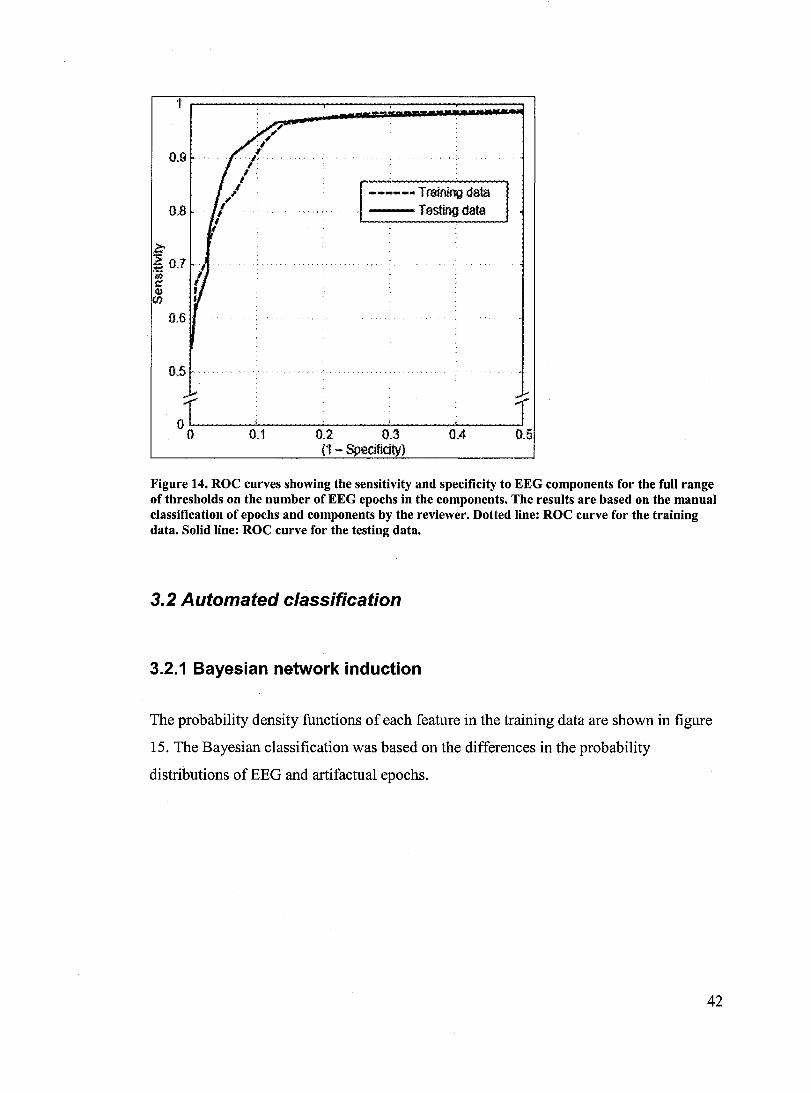
1
0.9 '
0.8
1:' 0> :::1 0.7 'l' .~ l Il) 1
U> 1
0.6
0.5 '
o Tt.....-_,'--, ----',----'----JI----'--',_--JJ o 0.1 0.2 0.3 OA 0.5
(1 - Spedfidty)
Figure 14. ROC curves showing the sensitivity and specificity to EEG components for the full range of thresholds on the number of EEG epochs in the components. The results are based on the manu al classification of epochs and components by the reviewer. Dotted Hne: ROC curve for the training data. Solid Hne: ROC curve for the testing data.
3.2 Automated classification
3.2.1 Bayesian network induction
The probability density functions of each feature in the training data are shown in figure
15. The Bayesian classification was based on the differences in the probability
distributions of EEG and artifactual epochs.
42

1
t ~
J 4
F
1
t 1 J
f ."
i ~ ct
2
'0 0.1 0.2 ().3 ReIatM~f~OaMl Hz
0.00 0.1 0.15 02 ~~ between 59aOO&1 Hz
-50 0 50 Olpole lI-COOIdînate (mm)
B 3il.--~~~
02 lM lUi 0,8 Refatîve ~ between laM 3 Hz
G
K o,oz,-----
C4r"'~_~~
li /\ , t \ , ,
f i , , '" 1 g. 1 .... 1 1
J
H
fO. -@o.
f~ 0.2
2 3 .(
o 6,r---rx------,
M UA 0.6 R_vtpower~ lSàI!d30Hz
1 0.51
~o. 'il
io,
10•
0.1
Projected va!Î8l1œ x lcf 10 20
Ne(lemropy
L M
~ lO.1
I~;
'0
"
' .. \. '" ......
"'-" .. .., 0.2 GA o.a
Rela!lIIe power between 30 aM 55 Hz
30
Figure 15. Probability density functions for the features in the training data for EEG (solid lines) and artifactual (dashed lin es) epochs. A-F: Relative power between 0-IHz, 1-3Hz, 3-15Hz, 15-30Hz, 30-55Hz, and 59-61Hz. G: Entropy ofthe power spectrum between 5 and 30 Hz. H: Projected variance ofthe reconstructed epochs. 1: Component negentropy. J-M: Equivalent dipole xyz-coordinates and eccentricity. These
~ dipole features were only considered if the residual variance of the dipole fitted on the component topography was less than 20%.

The distributions of the relative power between 15-30Hz and 30-55Hz for artifactual
epochs (Figure 15D and E) show that these features took on values that were either very
high, probably due to EMG artifacts, or very low, which would reflect movement and
EOG artifacts. On the other hand, for EEG epochs, these features took on values between
these two extremes. In particular, even though it is known that seizure activity can be
present between 15 and 30 Hz, the plot in figure 15D indicates that the power in this band
was mostly due to EMG artifacts.
In the 0-IHz and 1-3Hz bands (Figure 15A and B), EEG epochs again had a moderate
amount of power, while artifactual epochs took on more extreme values. Here, the high
power in these low-frequency bands was due to movement and EOG artifacts. There was
more overlap between the distributions ofEEG and artifacts than in the 15-30Hz and 30-
55Hz bands, because EMG artifacts were not easily distinguishable from seizure activity
at low frequencies.
The 3-15Hz band contained mostly seizure activity, since EMG artifacts were mostly
present at higher frequencies, while movement and EOG artifacts were characterized by
slower waves. Therefore, the two distributions shown in figure 15e can be distinguished
c1early, although there is still sorne significant overlap between EEG and artifactual
epochs.
The entropy of the power spectrum between 5 and 30 Hz was used as a measure ofthe
rhythmicity of the signal. As shown in figure 15G, artifacts tended to have high power
spectrum entropy, indicating a flat spectrum between 5 and 30 Hz. On the other hand,
seizure epochs often exhibited rhythmic activity in this frequency band, resulting in a
peak in the power spectrum and lower spectral entropy.
The probability distributions of the relative power between 59 and 61Hz and projected
variance are very similar for EEG and artifactual epochs (Figure 15F and H). For both
features, most of the values for EEG and artifacts are concentrated around zero. There
were a few sparse values greater than zero in the tails of the distributions for artifacts, but
44

these cannot be discemed in the graphs. This is because these features were selected to
identify very specific artifacts such as line noise and high-amplitude electrode artifacts
that only occurred rarely.
For the negentropy feature, the probability distribution of artifactual epochs has a heavier
tail than that ofEEG epochs (Figure 151). This reflects transient activity such as
movement artifact, whose distribution is highly non-Gaussian and thus has a high
negentropy value.
The xyz-coordinates of an equivalent dipole fitted to the spatial topography of a
component were added to the list of features whenever the residual variance of the fit was
less than 20%. The x-axis went from the posterior part to the anterior part of the head, the
y-axis went from right to left, and the z-axis went from the bottom to the top of the head.
The distributions ofthese coordinates (Figure 15J, K, and L) show that whenever EEG
epochs had a dipolar distribution, the position of the dipole tended to be close to the
origin of the coordinate system, which corresponded to the center of the head model. This
was expected, since the generators of EEG activity should be situated inside the brain. On
the other hand, the dipole xyz-coordinates for artifactual epochs have distributions with
several peaks, approximately corresponding to the grid-like arrangement of electrodes in
the 10-20 system (Figure 3). This is because many types of artifacts, such as the EMG,
have a very narrow spatial distribution, sometimes involving only a single channel. Fitted
dipoles will thus tend to be close to individual electrodes, yielding a distribution ofxyz
coordinates that matches the standard positions in the 10-20 system, although not aIl
electrodes were affected equaIly. For example, it is known that scalp muscle activity is
mostly confined to frontal and temporal locations (Goncharova et al., 2003).
Consequently, the distribution of artifacts in figure 15L does not have a peak in the
positive z-coordinates; this corresponds to locations at the top ofthe head that are not
affected as much by EMG contamination. Another observation is that the distribution for
artifactual epochs in figure 15J has a large peak at positive x-coordinates. This is
probably due to EOG artifacts, which were characterized by a dipole at the front of the
head.
45
The dipole eccentricity could be determined directly from its xyz-coordinates, but it was
still used as a feature because it provided a good separation between EEG and artifacts, as
can be seen in the distributions in figure 15M. Artifacts were mostly characterized by a
high dipole eccentricity, with a dipole position outside the brain near the surface of the
head model. In contrast, the dipole eccentricity for EEG epochs tended to correspond to a
position inside the brain. However, there is still a significant peak corresponding to a
dipole position near the surface of the head. This can be attributed to components that
were a mixture of EEG and artifactual activity. The spatial maps of these components
would be a combination of multiple topographies, but it is possible that they could still be
fitted with a dipole with less than 20% residual variance. In cases where artifacts were
more prominent than EEG activity in the mixtures, the resulting dipoles tended to be
closer to the topographies of the artifacts, with a position near the surface of the head.
However, epochs containing both EEG and artifactual activity were almost always
classified as EEG, even if the spatial topography of the components were fitted with
dipoles outside the brain. This is because a crucial feature of the system was its ability to
preserve EEG activity, even ifit meant that artifacts could not be entirely removed.
It should also be noted that even though scalp electrodes can only record cerebral activity
from the cortical surface, the fitted dipoles often had eccentricities corresponding to
deeper positions in the brain. This is because EEG activity does not originate from
discrete sources, but rather from a distributed arrangement of several synchronous
neurons, whose potential field can be approximated by a deeper single equivalent dipole.
While this means that the dipole model constitutes an inaccurate estimation of the
generator of the epileptic activity, it still provides useful information to distinguish
between EEG and artifactual components.
Two TAN Bayesian networks were induced from the training data for components with
either a dipolar or non-dipolar spatial topography (Figure 16). Every feature in the
network is a child node ofthe class attribute (EEG or artifact) and of at most one other
feature, as indicated by the correlation edges in the graph. Because of this restriction,
46
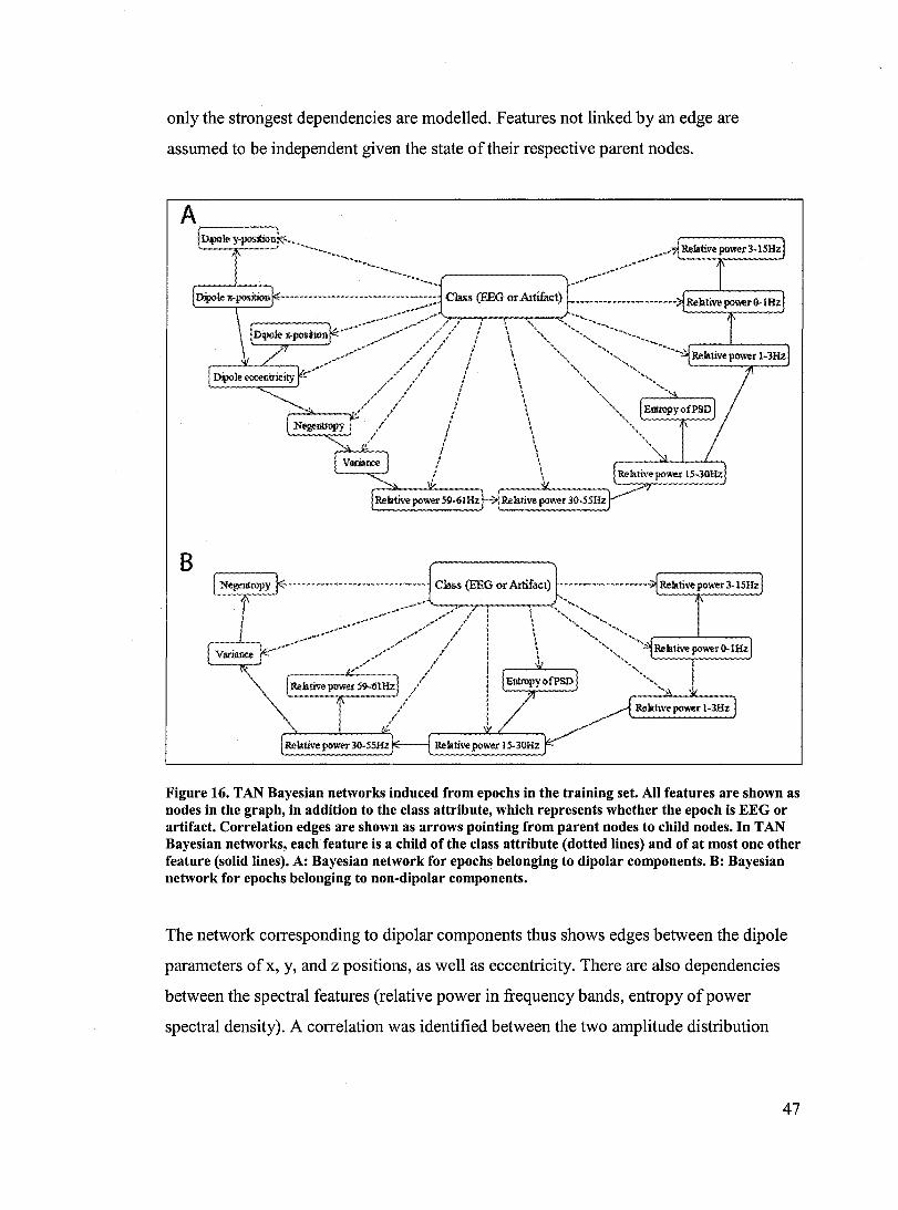
only the strongest dependencies are modelled. Features not linked by an edge are
assumed to be independent given the state of their respective parent nodes.
Relative power 30.55Hz
B .............................. Class (EEG orArtifact) •• > .................. Relativepower3-15Hz
Figure 16. TAN Bayesian networks induced from epochs in the training set. Ali features are shown as nodes in the graph, in addition to the class attribute, which represents whether the epoch is EEG or artifact. Correlation edges are shown as arrows pointing from parent nodes to child nodes. In TAN Bayesian networks, each feature is a child of the class attribute (dotted lines) and of at most one other feature (solid lines). A: Bayesian network for epochs belonging to dipolar components. B: Bayesian network for epochs belonging to non-dipolar components.
The network corresponding to dipolar components thus shows edges between the dipole
parameters of x, y, and z positions, as well as eccentricity. There are also dependencies
between the spectral features (relative power in frequency bands, entropy of power
spectral density). A correlation was identified between the two amplitude distribution
47

features of negentropy and variance, and also between the variance and the 60Hz activity
(relative power between 59 and 61Hz).
For non-dipolar components, the induced Bayesian network is almost identical after the
removal ofthe dipole features. The only other difference is that there is no longer a
correlation edge between the variance attribute and the power at 60Hz. Instead, there is a
dependency between the variance and the relative power between 30 and 55Hz.
It should be noted that among components that were manually classified as EEG in the
training set, 64.7% had a dipolar spatial distribution. In the validation set, 57.6% of the
EEG components were dipolar. A large number of components were a mixture of
cerebral and artifactual activity and had to be marked as EEG. These components were a
mixture of several sources and their spatial distribution thus could not be explained by a
single equivalent dipole. Because ofthis significant minority ofEEG components that
were non-dipolar, it was necessary to have the two separate Bayesian classifiers for the
automated classification task.
3.2.2 Classification results
The output ofthe Bayesian classifier was the probability that the epoch under
consideration represented EEG activity. To evaluate the performance of the classifier, an
epoch was considered to have been classified as EEG whenever the output probability
exceeded 50%. Comparing these results with the manual classification by the reviewer,
the system successfully recognized EEG epochs with an average sensitivity of 84.8% and
an average specificity of 85.3% in the training data. By using the same classifier on the
previously unseen validation set, the average sensitivity was 82.4% and the average
specificity was 83.3%.
The sum of the probabilities of epochs representing EEG activity was then used to
determine whether to reject or preserve each component. A threshold was selected by
constructing a ROC curve based on the classification results on the training data. The
48
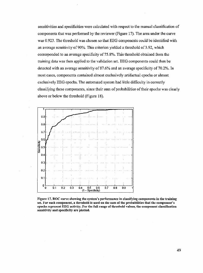
sensitivities and specificities were calculated with respect to the manu al classification of
components that was performed by the reviewer (Figure 17). The area under the curve
was 0.923. The threshold was chosen so that EEG components could be identified with
an average sensitivity of90%. This criterion yielded a threshold of3.92, which
corresponded to an average specificity of75.8%. This threshold obtained from the
training data was then applied to the validation set. EEG components could then be
detected with an average sensitivity of 87.6% and an average specificity of 70.2%. In
most cases, components contained almost exclusively artifactual epochs or almost
exclusively EEG epochs. The automated system had little difficulty in correctly
classifying these components, since their sum of probabilities of their epochs was clearly
above or below the threshold (Figure 18).
1
0.9
0.8·
~0.6 lli: ~ 0.5
~ 0.4
0.3
0.2
0.1
{) {) 0.1 0.2 0.3 0.4 0.5 0.6 0.7 0.8 0.9 (1 - Specîfldty)
Figure 17. ROC curve showing the system's performance in classifying components in the training set. For each component, a threshold is used on the sum of the probabilities that the component's epochs represent EEG activity. For the full range of threshold values, the component classification sensitivity and specificity are plotted.
49
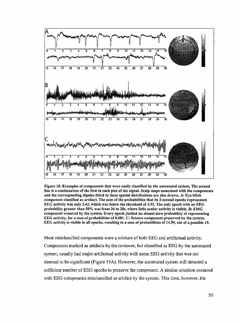
o 234 5
15 16 11 18 19 20 21 23 24
Figure 18. Examples of components that were easily classitied by the automated system. The second line is a continuation of the tirst in each plot of the signal. Scalp maps associated with the components and the corresponding dipoles titted to these spatial distributions are also drawn. A: Eye blink component ciassitied as artifact. The sum of the probabilities that its 2-second epochs represented EEG activity was only 2.42, which was below the threshold of 3.92. The only epoch with an EEG probability greater th an 50% was from 26 to 28s, where little ocular activity is visible. B: EMG component removed by the system. Every epoch yielded an al most-zero probability of representing EEG activity, for a sum of probabilities of 0.001. C: Seizure component preserved by the system. EEG activity is visible in ail epochs, resulting in a sum of probabilities of 14.99, out of a possible 15.
Most misc1assified components were a mixture ofboth EEG and artifactual activity.
Components marked as artifacts by the reviewer, but c1assified as EEG by the automated
system, usually had major artifactual activity with sorne EEG activity that was not
deemed to be significant (Figure 19A). However, the automated system still detected a
sufficient number of EEG epochs to preserve the component. A similar situation occurred
with EEG components misc1assified as artifact by the system. This time, however, the
50
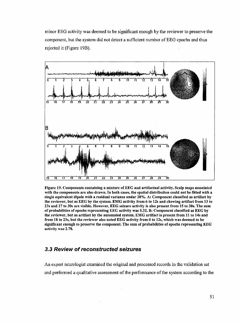
minor EEG activity was deemed to be significant enough by the reviewer to preserve the
component, but the system did not detect a sufficient number of EEG epochs and thus
rejected it (Figure 19B).
Figure 19. Components containing a mixture of EEG and artifactual activity. Scalp maps associated with the components are also drawn. In both cases, the spatial distribution could not be fitted with a single equivalent dipole with a residual variance under 20%. A: Component classified as artifact by the reviewer, but as EEG by the system. EMG activity from 6 to 12s and chewing artifact from 13 to 23s and 27 to 30s are visible. However, EEG seizure activity is also present from 15 to 30s. The sum of probabilities of epochs representing EEG activity was 5.32. B: Component classified as EEG by the reviewer, but as artifact by the automated system. EMG artifact is present from 11 to 14s and from 18 to 23s, but the reviewer also noted EEG activity from 0 to 12s, which was deemed to be significant enough to preserve the component. The sum of probabilities of epochs representing EEG activity was 2.78.
3.3 Review of reconstructed seizures
An expert neurologist examined the original and processed records in the validation set
and performed a qualitative assessment ofthe performance of the system according to the
51

criteria shown previously in table 3. The reviewer scores for each seizure record are
shown in table 4.
Patient number Artifacts in the original Artifacts removal EEGremoval record
1 Almostnone Similar or worse Ali preserved (5 seizures) Few Similar or worse Ali preserved
Few Minor improvement Ali preserved Few Minor improvement Minor attenuation Few Minor improvement Minor attenuation
2 Significant Major improvement Ali preserved (2 seizures) Significant Major improvement Minor attenuation
3 Significant Minor improvement Ali preserved (3 seizures) Significant Major improvement Minor attenuation
Significant Similar or worse Ali preserved 4 Significant Major improvement Major attenuation
(5 seizures) Significant Major improvement Major attenuation Significant Minor improvement Major attenuation Significant Major improvement Mostly preserved
Considerable Major improvement Minor attenuation 5 Significant Minor improvement Minor attenuation
(18 seizures) Considerable Similar or worse Ali preserved Almostnone Similar or worse Ali preserved Considerable Similar or worse Ali preserved Almostnone Similar or worse Ali preserved Significant Similar or worse Ali preserved
Considerable Minor improvement Ali preserved Few Similar or worse Ali preserved Few Minor improvement Ali preserved
Considerable Similar or worse Ali preserved Significant Similar or worse Ali preserved
Considerable Similar or worse Major attenuation Considerable Minor improvement Ali preserved
Few Similar or worse Ali preserved Few Mostly removed Ali preserved Few Similar or worse Ali preserved
Considerable Similar or worse Ali preserved Considerable Similar or worse Ali preserved
6 Significant Similar or worse Ali preserved (3 seizures) Considerable Minor improvement Ali preserved
Significant Similar or worse Ali preserved 7 Significant Major improvement Mostly preserved
(3 seizures) Significant Major improvement Mostly preserved Significant Major improvement Ali preserved
8 Considerable Major improvement Major attenuation (3 seizures) Few Major improvement Ali preserved
Significant Major improvement AII~eserved 9 Considerable Major improvement Ali preserved
(4 seizures) Considerable Major improvement Ali preserved Significant Minor improvement Minor attenuation Significant Minor improvement Ali preserved
10 Almostnone Similar or worse Ali preserved (3 seizures) Few Similar or worse Minor attenuation
Significant Mostly removed Ali preserved
Table 4. Qualitative classification of each record in the validation dataset by an expert neurologist. For each review parameter, the reviewer selected a scoring category as outlined in table 3.
52
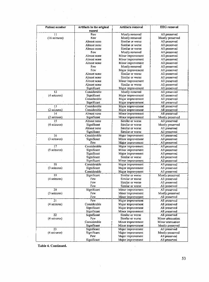
Patient number Artifacts in the original Artifacts removal EEG removal record
Il Few Mostly removed Ali preserved (16 seizures) Few Mostly removed Mostly preserved
Almostnone Similar or worse Ali preserved Almostnone Similar or worse Ali preserved Almost none Similar or worse Ali preserved
Few Mostly removed Ali preserved Almostnone Minor improvement Ali preserved Almostnone Minor improvement Ali preserved Almostnone Minor improvement Ali preserved
Few Mostly removed Ali preserved Few Major improvement Ali preserved
Almostnone Similar or worse Ali preserved Almostnone Similar or worse Ali preserved Almostnone Minorimprovement Ali preserved Almostnone Similar or worse Ali preserved Significant Major improvement Ali preserved
12 Considerable Mostly removed Ali preserved (4 seizures) Significant Major improvement Ali preserved
Considerable Major improvement Ali preserved Significant Major improvement Ali preserved
13 Considerable Major improvement Ali preserved (2 seizures) Considerable Maior improvement Ali preserved
14 Almostnone Minor improvement Ali preserved (2 seizures) Significant Minor improvement Mostly preserved
15 Almostnone Similar or worse Ali preserved (4 seizures) Significant Similar or worse Mostly preserved
Almostnone Similar or worse Ali preserved Significant Similar or worse Ali preserved
16 Considerable Major improvement AlI preserved (3 seizures) Significant Minor improvement Ali preserved
Few Major improvement Ali preserved 17 Considerable Major improvement AlI preserved
(5 seizures) Significant Minor improvement AlI preserved Significant Major improvement AlI preserved Significant Similar or worse Ali preserved Significant Minor improvement Ali preserved
18 Considerable Major improvement Ali preserved (3 seizures) Significant Major improvement Ali preserved
Considerable Major improvement Ali preserved 19 Significant Similar or worse Mostly preserved
(4 seizures) Few Similar or worse Ali preserved Few Similar or worse Ali preserved Few Similar or worse AlI preserved
20 Significant Minor improvement Ali preserved (3 seizures) Few Minor improvement Mostly preserved
Few Minor improvement AlI preserved 21 Few Major improvement Ali preserved
(4 seizures) Considerable Major improvement Ali preserved Significant Major improvement Ali preserved Significant Minor improvement Ali preserved
22 Significant Similar or worse Ali preserved (4 seizures) Few Similar or worse Minor attenuation
Considerable Minor improvement Minor attenuation Significant Minor improvement Mostly preserved
23 Significant Major improvement Ali preserved (4 seizures) Significant Major improvement Mostly preserved
Few Major improvement AlI preserved Significant Major improvement Ali preserved
Table 4. Continued.
53
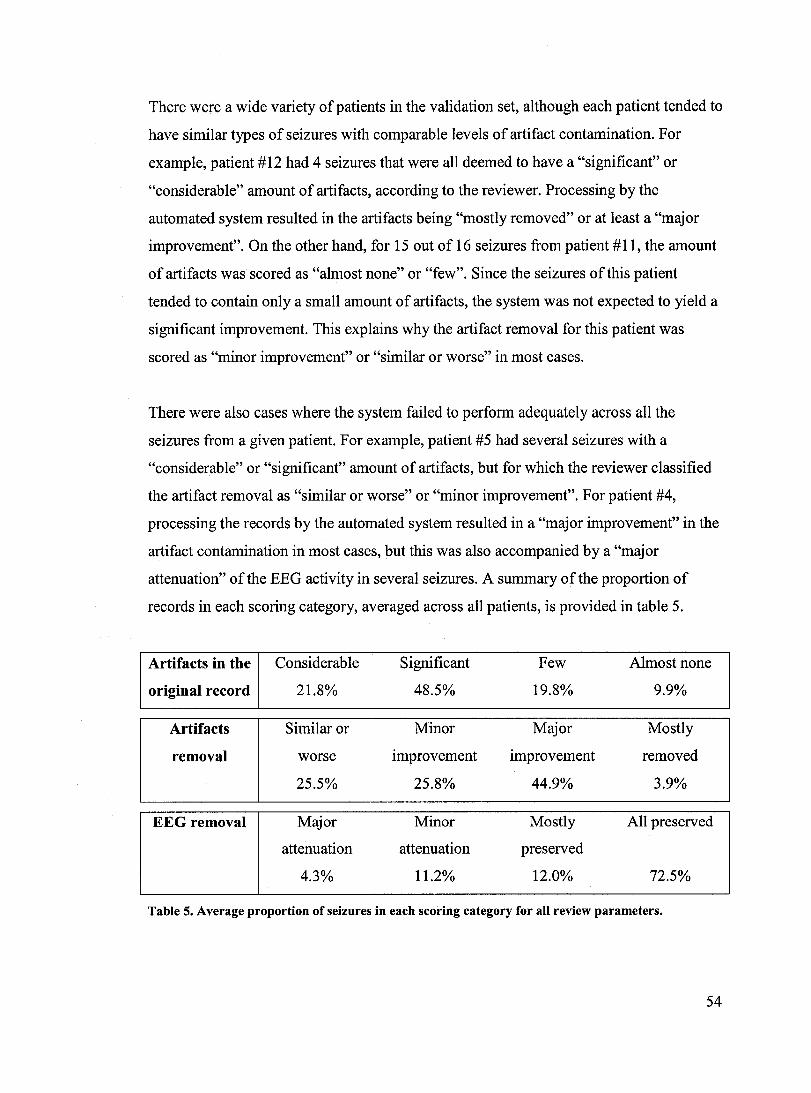
There were a wide variety of patients in the validation set, although each patient tended to
have similar types of seizures with comparable levels of artifact contamination. For
example, patient #12 had 4 seizures that were all deemed to have a "significant" or
"considerable" amount of artifacts, according to the reviewer. Processing by the
automated system resulted in the artifacts being "mostly removed" or at least a "major
improvement". On the other hand, for 15 out of 16 seizures from patient #11, the amount
of artifacts was scored as "almost none" or "few". Since the seizures ofthis patient
tended to contain only a small amount of artifacts, the system was not expected to yield a
significant improvement. This explains why the artifact removal for this patient was
scored as "minor improvement" or "similar or worse" in most cases.
There were also cases where the system failed to perform adequately across all the
seizures from a given patient. For example, patient #5 had severai seizures with a
"considerable" or "significant" amount of artifacts, but for which the reviewer c1assified
the artifact removal as "similar or worse" or "minor improvement". For patient #4,
processing the records by the automated system resulted in a "major improvement" in the
artifact contamination in most cases, but this was aiso accompanied by a "major
attenuation" of the EEG activity in several seizures. A summary of the proportion of
records in each scoring category, averaged across all patients, is provided in table 5.
Artifacts in the Considerable Significant Few Almostnone
original record 21.8% 48.5% 19.8% 9.9%
Artifacts Similar or Minor Major Mostly
removal worse improvement improvement removed
25.5% 25.8% 44.9% 3.9%
EEG removal Major Minor Mostly AlI preserved
attenuation attenuation preserved
4.3% 11.2% 12.0% 72.5%
Table 5. Average proportion of seizures in each scoring category for ail review parameters.
54
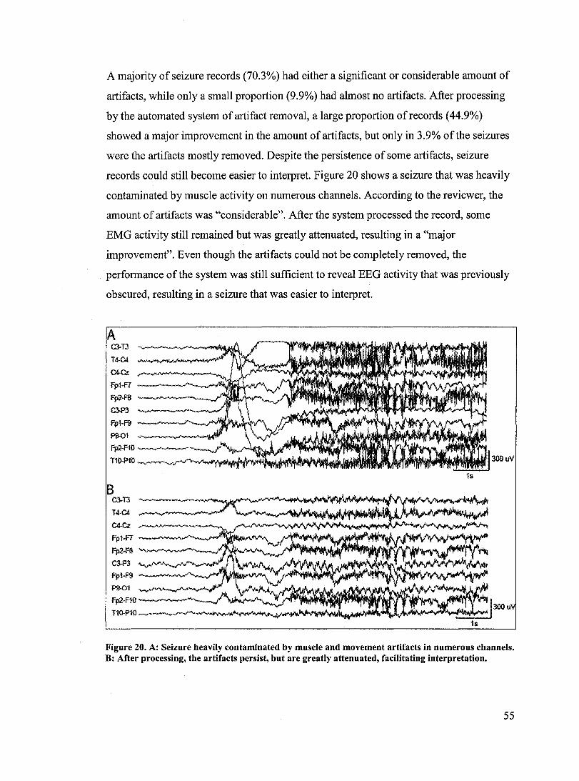
A majority of seizure records (70.3%) had either a significant or considerable amount of
artifacts, while only a small proportion (9.9%) had almost no artifacts. After processing
by the automated system of artifact removal, a large proportion of records (44.9%)
showed a major improvement in the amount of artifacts, but only in 3.9% ofthe seizures
were the artifacts mostly removed. Despite the persistence of sorne artifacts, seizure
records could still become easier to interpret. Figure 20 shows a seizure that was heavily
contaminated by muscle activity on numerous channels. According to the reviewer, the
amount of artifacts was "considerable". After the system processed the record, sorne
EMG activity still remained but was greatly attenuated, resulting in a "major
improvement". Even though the artifacts could not be completely removed, the
performance of the system was still sufficient to reveal EEG activity that was previously
obscured, resulting in a seizure that was easier to interpret.
A (;3..13
T4·C4
C4-Cz.
fp1-F]
fp2-F8
C3-P3
Fpl-F9
f'9.01
fp2-F'HI
T10-P10 300 uV
B C3-13 ~
T4-C4
C4-Cz
Fp'1-F1
Fp2-f3
Figure 20. A: Seizure heavily contaminated by muscle and movement artifacts in numerous channels. B: After processing, the artifacts persist, but are greatly attenuated, facilitating interpretation.
55
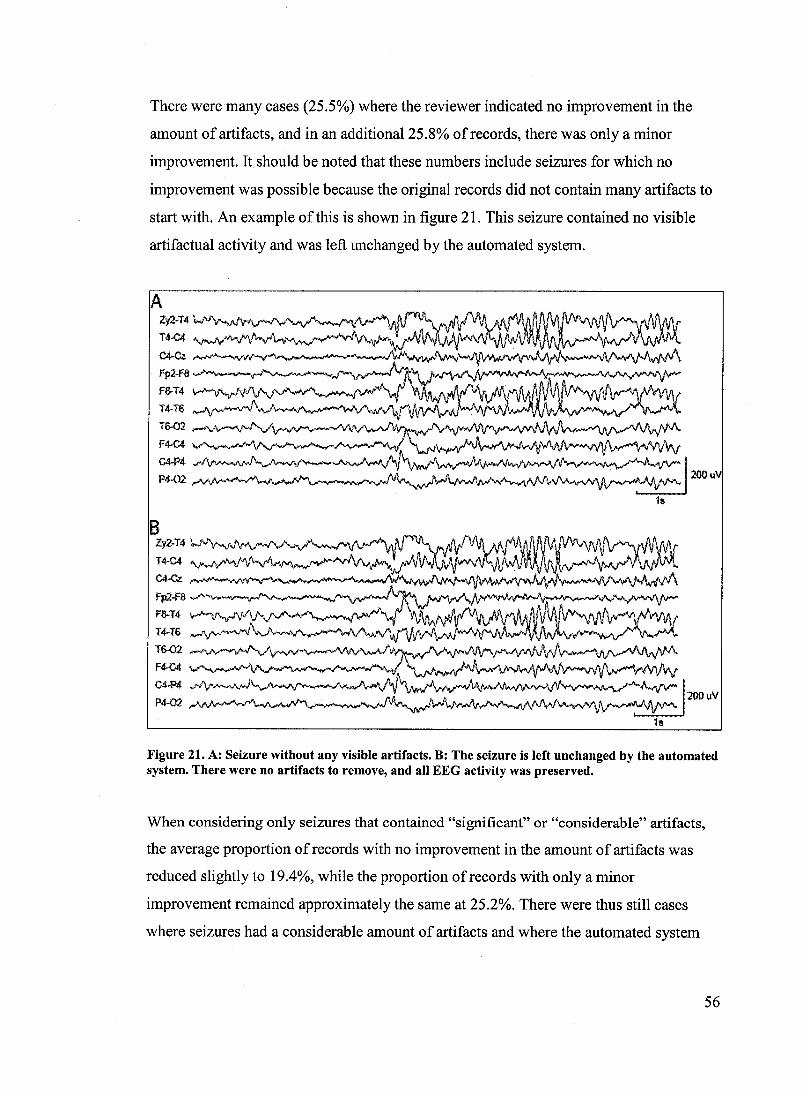
There were many cases (25.5%) where the reviewer indicated no improvement in the
amount of artifacts, and in an additionaI25.8% ofrecords, there was only a minor
improvement. It should be noted that these numbers inc1ude seizures for which no
improvement was possible because the original records did not contain many artifacts to
start with. An example of this is shown in figure 21. This seizure contained no visible
artifactual activity and was left unchanged by the automated system.
A Z)'2-T4 \
T4-04
~~ ~~~~~~~~--~~
T4-04 ~~"\ V'V"~'_.J
~.~ ~~~~~~~~--~~
F~~a~~~~r~~~~~
Figure 21. A: Seizure without any visible artifacts. B: The seizure is left unchanged by the automated system. There were no artifacts to remove, and ail EEG activity was preserved.
When considering only seizures that contained "significant" or "considerable" artifacts,
the average proportion of records with no improvement in the amount of artifacts was
reduced slightly to 19.4%, while the proportion of records with only a minor
improvement remained approximately the same at 25.2%. There were thus still cases
where seizures had a considerable amount of artifacts and where the automated system
56
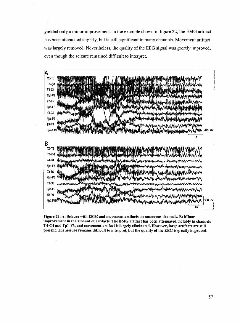
yielded only a minor improvement. In the example shown in figure 22, the EMG artifact
has been attenuated slightly, but is still significant in many channels. Movement artifact
was largely removed. Nevertheless, the quality ofthe EEG signal was greatly improved,
even though the seizure remained difficult to interpret.
A
300 uV
Figure 22. A: Seizure with EMG and rnovernent artifacts on nurnerous channels. B: Minor irnprovement in the arnount of artifacts. The EMG artifact has been attenuated, notably in channels T4-C4 and Fpl-F3, and rnovernent artifact is largely eliminated. However, large artifacts are still present. The seizure rernains difficult to interpret, but the quality of the EEG is greatly irnproved.
57
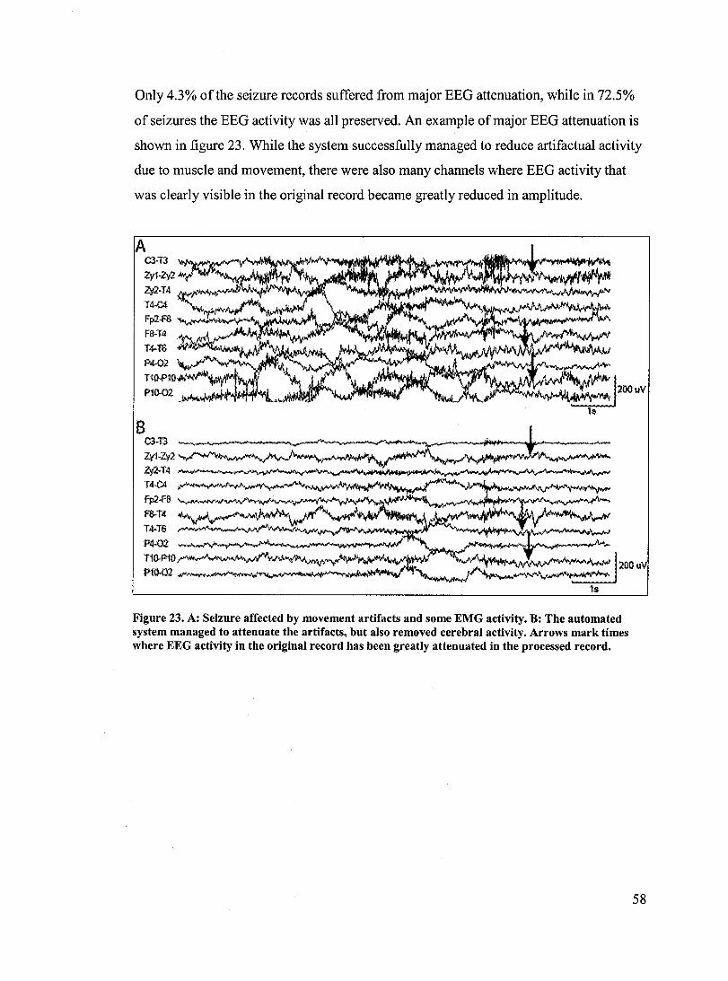
Only 4.3% of the seizure records suffered from major EEG attenuation, while in 72.5%
of seizures the EEG activity was all preserved. An example of major EEG attenuation is
shown in figure 23. While the system successfully managed to reduce artifactual activity
due to muscle and movement, there were also many channels where EEG activity that
was clearly visible in the original record became greatly reduced in amplitude.
A C3-T3
P4-02 T1o-P10.MWlr""I ..
Pl0-02 J!<I"\!~i" .. "
Figure 23. A: Seizure affected by movement artifacts and some EMG activity. B: The automated system managed to attenuate the artifacts, but also removed cerebral activity. Arrows mark times where EEG activity in the original record has been greatly attenuated in the processed record.
58

Figure 24 shows an example of minor EEG attenuation. In this case, the EEG in the
processed record has a slightly reduced amplitude, but remains clearly visible in most
channels.
A Zy2-T4
C4-Cz
Fpl.f1
T3-T5
F8-T4
T4-T6
T6-02
C4-P4
P4-02
B 2y2-14
~,~~~~~~~~~~~~~~~~~~~~~~~~~~~
f8-T4 ... , ....... ~4"~bt..W"'~M ,...,,.-l'#' ................ J''I'I',~~~ .............. ,. 14-16 f,I.I..v'IMM~fIM,j
16-02
~P4 ~~~~~~~
1&
Figure 24. A: Seizure contaminated by sorne minor EMG activity in various channels and an electrode artifact in channel Fpl-F7. B: ACter processing by the automated system, the amount of artifacts is reduced, but the EEG also suffers from minor attenuation. Arrows indicate times where seizure dis charges in the original record are still visible in the processed record, although with a reduced amplitude.
59
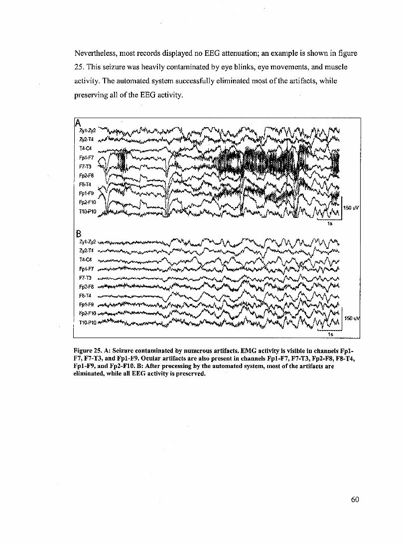
Nevertheless, most records displayed no EEG attenuation; an example is shown in figure
25. This seizure was heavily contaminated by eye blinks, eye movements, and muscle
activity. The automated system successfully eliminated most ofthe artifacts, while
preserving all of the EEG activity.
A è{t-Zy2
Zy2-T4
T4-C4
Fp1-F7
F7.j3
Fp2.f8
f'8.T4
Fp1.f9
Fp2.fl0
11o.P10
B Zy1-Zy2
Zy2-T4
T4-C4
f7.j3
Fp2.FIl
fl3-T4
Fp1..f9
Fp2-Fl0
T1o.Pl0~
1s
Figure 25. A: Seizure contaminated by numerous artifacts. EMG activity is visible in channels FplF7, F7-T3, and Fpl-F9. Ocular artifacts are also present in channels Fpl-F7, F7-T3, Fp2-F8, F8-T4, Fpl-F9, and Fp2-FIO. B: ACter processing by the automated system, most of the artifacts are eliminated, while ail EEG activity is preserved.
60
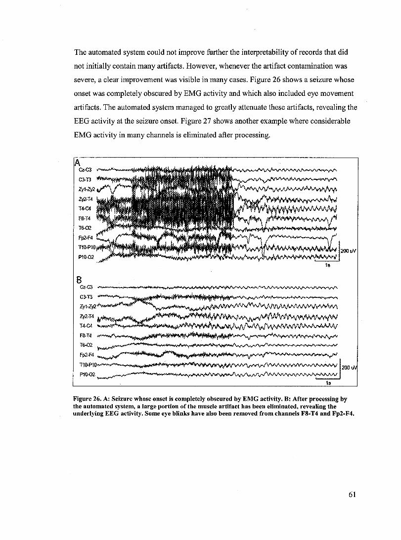
The automated system could not improve further the interpretability of records that did
not initially contain many artifacts. However, whenever the artifact contamination was
severe, a c1ear improvement was visible in many cases. Figure 26 shows a seizure whose
onset was completely obscured by EMG activity and which also inc1uded eye movement
artifacts. The automated system managed to greatly attenuate these artifacts, revealing the
EEG activity at the seizure onset. Figure 27 shows another example where considerable
EMG activity in many channels is eliminated after processing.
Zy2-T4
T4-C4
Fa-T4
B Cz-Q
1$
C3-T3 ~
Zy1-Z'/2 ~V'\
Zy2-T4~~ .~~~~ T4-C4 ~jl:~~~v\,..NW\tV,NV'4VVV''''~v F~~ ~~~~~~~~~~~~~~~ T6-02
Fp2.f4
T1().p10,~"""V" ...... ~~ .... ~~..,...W'I!r""'~M~~W'\NV'\
P10-02
uV
Figure 26. A: Seizure whose onset is completely obscured by EMG activity. B: After processing by the automated system, a large portion of the muscle artifact has been eliminated, revealing the underlying EEG activity. Sorne eye blinks have also been removed from channels F8-T4 and Fp2-F4.
61
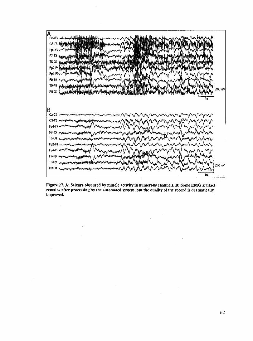
B Cz~r-~~~~w-~~~~ __ ~
~n~~~~~~~~~~~~Al
Fp1·R-~"""'''*''''''''''''
R-Tl ~~~~~1111"11\
T>Ol ~~~~~~~~~~~~~
Fpl·F4"-'...."... __ ....... """" ....... II'i\.,..N<" ....... """"..,...,.","""
Fp1.f9-~"""' .... .,.,..-...
F9-T9 "...... ........ .-M..JI<!iIIN'l1!';o
T~~~~~~~~~~~~
~1 ~~~~~~~~~~~
Figure 27. A: Seizure obscured by muscle activity in numerous channels. B: Some EMG artifact remains aCter processing by the automated system, but the quality of the record is dramatically improved.
62

4. Discussion
4. 1 Arlifact separation by ICA
It is very difficult to demonstrate that the components extracted by ICA correspond to the
individual generators of the recorded signal, because the actual time courses ofthese
sources cannot be measured directly. Nevertheless, simulation studies support the use of
ICA to separate artificial sources from synthetic EEG signaIs (Barbati et al., 2004).
Equivalent dipoles fitted to sources extracted by ICA have also been shown to
approximately match the fields measured by intracranial electrodes (Kobayashi et al.,
2001). Consequently, ICA applied to scalp EEG was expected to successfully separate
artifactual sources into distinct components. However, this separation is usually not ideal
because EEG recordings tend to violate one of the fundamental assumptions of ICA,
namely that the number of sources should be equal to the number of recording channels
(Makeig et al., 1996b). It is impossible to determine the exact number ofindependent
brain signaIs being recorded on the scalp, in addition to the numerous extra-cerebral
sources ofnoise and artifacts. Nevertheless, it has been shown that ICA tends to separate
the strongest sources, while weaker generators are scattered into multiple components
(Makeig et al., 1996a). In this case, each ICA component is a mixture of a separated
strong source with additional contributions from weaker sources with similar spatial
distributions.
However, in the case ofEEG heavily contaminated by artifacts, sorne components might
be a mixture of multiple strong sources. The mixture of these strong sources will tend to
be normally distributed, which would make the ICA decomposition unpredictable
(Hyvarinen et al., 2001). ICA cannot separate sources with a Gaussian distribution;
however, ICA should still be able to isolate sources ofrhythmic epileptic activity, or
transient artifactual sources such as the EOG. On the other hand, the EMG signal is the
result of the summation of the activity from several asynchronous muscle cells and
should thus tend toward a Gaussian distribution. It has indeed been reported that the
63
perfonnance oflCA may degrade when trying to remove EMG artifacts from the EEG
(Nam et al., 2002; Urrestarazu et al., 2004). The probability distributions ofthe
negentropy feature shown in figure 151 indicate that several components had a
negentropy close to zero, which corresponds to Gaussian distributions. These components
probably were the result of mixtures of several sources, which might contain both
significant EEG and artifactual activity. In this case, artifacts could not be entirely
removed since this would have also eliminated EEG activity. Nevertheless, ICA can still
successfully isolate components with distributions that deviate only slightly from
nonnality (Jung et al., 2000c). The system was thus still able to remove several artifactual
components from the seizure recordings. It might be interesting, however, to explore
other methods ofblind source separation to extract muscle activity from EEG recordings.
For Gaussian signaIs, statistical independence is equivalent to uncorrelatedness and thus
does not provide any additional infonnation allowing the separation of the sources. By
introducing additional constraints to the algorithm, it might be possible to improve the
separation of Gaussian sources. For example, the method of canonical correlation
analysis (CCA) attempts to decorrelate the mixed signaIs with constraints on their
auto correlation structure (Borga and Knutsson, 2001). This approach could be useful to
extract signaIs such as the EMG that have a noise-like appearance with very little
autocorrelation.
During the visual inspection of the seizure recordings in the training data, the number of
epochs identified as EEG varied greatly for the various components. There were many
instances of components that were not entirely composed of either EEG or artifactual
epochs. The de ci sion on whether to preserve or reject these components was left to the
subjective judgment of the reviewer. The automated system was thus likely to reflect this;
in the future, a more accurate gold standard could be obtained by combining the results
from multiple reviewers.
Components were preserved whenever they contained EEG activity that was deemed to
be significant. Since ICA components were assumed to represent a mixture of spatially
stationary sources, it was unlikely that significant EEG activity would only be present in
64
a few epochs. Using a threshold on the number ofEEG epochs should thus be an
appropriate criterion to preserve or remove components. This is demonstrated by the
constructed ROC curve; the area under the curve was used as a measure of the
threshold's discrimination power between EEG and artifactual components (Swets,
1988). For the training set, the area under the ROC curve was 0.966, indicating that a
threshold on the number of EEG epochs can provide excellent separation between the
two types of components.
4.2 TAN Bayesian classification
The use of a Bayesian formulation to classify EEG signaIs has previously been applied
successfully in seizure detection systems (Saab and Gotman, 2005; Grewal and Gotman,
2005). This framework was refined here by introducing the TAN Bayesian network
structure to allow the use of a larger number of features. The induced TAN Bayesian
networks show the dependencies that were modelled to estimate the PDFs of the various
features. For example, electrode artifacts tended to be associated with both a high
variance and activity at 60Hz. There was thus a correlation edge between those two
features, but only for the dipolar case, since electrode artifacts mostly affected a single
channel and could therefore be fitted with a dipole at the electrode location. In the non
dipolar case, high amplitude was more likely to be associated with EMG activity, hence
the edge between the features ofvariance and relative power between 30 and 55Hz.
Despite these modelled dependencies, there are also pairs of features that were
incorrectly assumed to be independent. In particular, all the features of relative power in
various frequency bands are mutually dependent and should therefore have correlation
edges between every pair ofthem. A similar reasoning applies for all features related to
dipole position. However, the TAN Bayesian structure restricts the dependencies to
ensure that the classification is computationally tractable. Although this will cause
inaccuracies in the output probabilities of the system, it has been shown that TAN
Bayesian networks can offer a performance comparable or better than other state-of-the
art classifiers such as C4.5 decision trees (Friedman et al., 1997).
65
In many cases, it was unclear whether an epoch represented EEG activity or artifact. This
can account for a lot ofvariability in the gold standard based on the reviewer's markings.
In a study on EMG artifact detection in the EEG, van de Velde et al. evaluated the
performance of an expert reviewer marking EMG artifacts on the same recordings twice
(van de Velde et al., 1998). Using l-second epochs, the reviewer correctly identified
82.6% ofEMG epochs that were marked on a previous mn with the same dataset. AIso,
92.1 % of non-EMG epochs were detected during the second mn. In another study by the
same group, two expert reviewers identified artifacts ofvarious types in long-term EEG
recordings, using lü-second epochs (van de Velde et al., 1999). On average, 76% of the
artifacts marked by one expert were also marked by the other. For non-artifactual epochs,
the average consensus was typically higher than 95%.
These measures of intra- and inter-expert variability provide a benchmark on the
performance ofthe automated system. It successfully detected 82.4% ofEEG epochs and
83.3% of artifactual epochs in the validation set. Sensitivity to artifacts is thus similar to
the experts' performance. This success rate may be partly due to the fact that the analysis
was performed on ICA components, where strong sources are separated into individual
signaIs, rather than on raw EEG. On the other hand, the detection ofEEG epochs was
worse than the experts' performance. However, van de Velde et al. have attributed their
high inter-expert consensus on EEG epochs to the low occurrence of artifacts (van de
Velde et al., 1999). The prolonged EEG recordings used in their study contained lengthy
periods of artifact-free data. This was not the case for the ictal EEG used in the current
study, which tended to be heavily contaminated by artifacts because epileptic seizures are
often accompanied by involuntary movements and automatisms affecting the EEG.
It should also be noted that the performance of the classifier deteriorated little between
the training set and the validation set. This indicates that the classifier was sufficiently
general to be used on a wide variety of seizure recordings from patients who had not been
seen previously.
66
4.3 Component classification
The area under the ROC curve for the number of EEG epochs determining whether to
preserve or reject ICA components was 0.923, indicating that using a threshold would
provide a good separation between the two types of components. It was crucial to
preserve the EEG activity from the recording, hence the requirement for high sensitivity
to EEG components in the training data. However, excessively increasing the sensitivity
would result in a loss of specificity, meaning that the system would preserve all EEG
activity, but would not remove any artifacts. By experimenting on the training data, it
was found that a sensitivity of 90% preserved most of EEG activity while still removing a
significant amount of artifacts. The corresponding threshold of 3.92, out of a maximum
of 15 epochs per component, was consistent with the epoch classification accuracy of the
system. A lower threshold would not be sufficient to detect significant EEG activity,
since a few EEG epoch detections might be entirely due to the classification error rate.
In the validation set, the identification ofEEG components was performed with a
sensitivity of 87.6% and specificity of 70.2%, which were only slightly worse than the
inter-expert performance described above. A significant proportion of artifactual
components can thus be removed by the automated system, while still preserving most of
the EEG activity. Again, there was only a slight deterioration of the performance of the
system when applied to the validation set compared to the training set, demonstrating the
system's generalization ability.
The two types of misclassifications (EEG components classified as artifact and vice
versa) occurred with similar types of components. In most cases, the components were a
mixture of artifact and sorne minor EEG activity. Whether to preserve or reject the
component depended on the subjective judgment ofthe reviewer, which suffered from
sorne inherent variability. The error rate of the classifier can thus be partly attributed to
these inconsistencies in the reviewer markings in the training data.
67
4.4 Analysis of reconsfrucfed seizures
There are no absolute measures of the ease of interpretation of a seizure recording, so a
subjective method had to be designed. This approach was similar to the one used by
Urrestarazu et al. (Urrestarazu et al., 2004), who evaluated the quality ofEEG
reconstructed after removing visually selected artifactual components extracted by ICA.
On the other hand, the current study used a completely automated system to select the
appropriate components.
During the qualitative evaluation process by the reviewer, both the original and the
processed records were examined simultaneously. This method was necessary to evaluate
the preservation of EEG activity by the automated system. Seizures can exhibit a wide
variety of EEG patterns, ranging from high-amplitude rhythms to more subtle discharges
(Blume et al., 1984). There is consequently no clear measure of the amount ofEEG
activity, and any attenuation can thus only be recognized by directly comparing the
original and processed signaIs.
The reviewer indicated that most seizures were contaminated by a significant amount of
artifacts. This is typical ofictal EEG (Gotman, 1999), which is often accompanied by
involuntary clinical symptoms that are responsible for sorne of the artifacts appearing on
the EEG. The artifacts often complicate the seizure interpretation, especially if they are
present at the time of the seizure onset. In this case, the seizure records were thus likely
to benefit greatly from the automated system of artifact removal. The system could be
useful in removing doubts regarding the analysis of a seizure, confirming the
interpretation from the original unprocessed record. The reconstructed EEG record could
also help identify cerebral activity that might otherwise be difficult to notice in the
original EEG. The automated system would thus be intended for seizures that are difficult
to interpret due to a large number of artifacts obscuring the EEG.
68
4.5 Future Work
The system provides an effective way of automatically removing several types of artifacts
from ictal scalp EEG to facilitate seizure interpretation by clinicians, as opposed to
methods only suitable for specific artifacts. In particular, digital filters, which are
currently in common use in clinical applications, can only provide a partial reduction of
artifacts. Nevertheless, filters could be used in conjunction with the automated system in
cases where ICA fails to provide perfect separation between EEG and artifactual activity,
particularly the EMG. It has been shown previously (Urrestarazu et al., 2004) that filters
can be used as a good complement to ICA methods, further improving the quality of ictal
EEG recordings. An eventual implementation of the system in a clinical setting should
thus provide a combined analysis using digital filters as weIl.
A current limitation of the system is that there are occasional instances where significant
EEG activity is removed after processing the seizure records. This is caused by an
erroneous selection of the components to be removed by the automated classifier. In this
case, electroencephalographers cannot rely on the processed records and must analyze the
EEG based solely on the original signal. However, it would seem wasteful to ignore the
information provided by the automated classifier. In particular, the system provides a
ranking of the components according to the sum of the probabilities that their epochs
represent EEG activity. Rather than using a fixed threshold on this sum of probabilities to
classify the components, it might be possible to allow users to fine-tune this value for
each record. Whenever significant EEG activity is removed by the system, a lower
threshold on the EEG probability can be used to preserve additional components, but still
remove an important amount of artifacts. Similarly, ifEEG activity is unaffected by the
system while significant artifacts remain in the processed records, a higher threshold can
be used. The tuning of the threshold value would require only minimal manual
intervention; this approach would still save users from the tedious visual examination of
the components extracted by ICA. However, it is also possible that components could
become improperly rejected or retained, while they were initially classified correctly
69
using the original threshold. In this case, adjusting the threshold would cause the EEG
quality to deteriorate.
In the future, the system could be extended to integrate a measure of the significance of
each identified artifactual epoch. Currently, features extracted from component epochs
are only used to assert the presence or absence of artifacts, without considering their
amplitude. However, a component might contain several artifactual epochs with a high
probability, but oflow projected amplitude. Removing this component would not
significantly alter the reconstructed EEG, especially ifthere are other high-amplitude
artifactual components affecting the same channels. It might thus be preferable for the
system to focus on the most significant components.
4.6 Conclusion
The main difficulty with ICA-based methods for artifact removal in ictal EEG is the
tedious visual selection of artifactual components. The proposed system can automate
this process, thus allowing this approach to be used in a practical way in a clinical setting.
The use of a TAN Bayesian framework allowed a large number of features to be used in
the classification task. This yielded a classifier with a performance that was only slightly
worse than the errors that would be expected from human expert variability. Therefore,
this system is expected to improve the interpretability of seizures recorded on scalp EEG
by removing a significant portion of artifacts obscuring the EEG activity.
70
References
Barbati G, Porcaro C, Zappasodi F, Rossini PM, Tecchio F. Optimization of an independent component analysis approach for artifact identification and removal in magnetoencephalographic signaIs. Clin.Neurophysiol. 2004; 115: 1220-1232.
Bell AJ, Sejnowski TJ. An information-maximization approach to blind separation and blind deconvolution. Neural Comput. 1995; 7: 1129-1159.
Blume WT, Young GB, Lemieux JF. EEG morphology ofpartial epileptic seizures. Electroencephalogr.Clin.Neurophysiol. 1984; 57: 295-302.
Borga, M. and Knutsson, H. A Canonical Correlation Approach to Blind Source Separation. Linkoping University: Department of Biomedical Engineering; 2001. Report No.: LiU-IMT-EX-0062.
Cardoso JF. High-order contrasts for independent component analysis. Neural Comput. 1999; Il: 157-192.
Cormen, T. H., Leiserson, C. E., Rivest, R. L. Introduction to Aigorithms, Cambridge, MA: MIT Press, 1990.
Delorme, A., Makeig, S., Sejnowski, T. Automatic artifact rejection for EEG data using high-order statistics and Independent Component Analysis. In: Proceedings Of 3rd International Independent Component Analysis and Blind Source Decomposition Conference; San Diego; 2001; p. 457-462.
Delorme A, Makeig S. EEGLAB: an open source toolbox for analysis of single-trial EEG dynamics including independent component analysis. J.Neurosci.Methods 2004; 134: 9-21.
Delsanto, S., Lamberti, F., Montrucchio, B. Automatic ocular artifact rejection based on independent component analysis and eyeblink detection. In: Proceedings of the lst International IEEE EMBS Conference on Neural Engineering; Capri Island, Italy; 2003; p.309-312.
Farabee, M. J. On-Line Biology Book. http://www.emc.maricopa.edu/faculty/farabee/BIOBKlBioBookTOC.html. Last accessed on November Il,2005.
Fayyad, u., Irani, K. Multi-interval discretization of continuous-valued attributes for classification learning. In: Proceedings of 13th International Joint Conference on Artificial Intelligence; 1993; p. 1022-1029.
71
Flanagan D, Agarwal R, Wang YH, Gotman J. Improvement in the performance of automated spike detection using dipole source features for artefact rejection. Clin.Neurophysiol. 2003; 114: 38-49.
Friedman N, Geiger D, Goldszmidt M. Bayesian Network Classifiers. Mach.Leam. 1997; 29: 131-163.
Gasser T, Sroka L, Mocks J. The transfer ofEOG activity into the EEG for eyes open and closed. Electroencephalogr.Clin.Neurophysiol. 1985; 61: 181-193.
Gloor P. Neuronal generators and the problem oflocalization in electroencephalography: application of volume conductor theory to electroencephalography. J.Clin.Neurophysioi. 1985; 2: 327-354.
Goncharova II, McFarland DJ, Vaughan TM, Wolpaw JR. EMG contamination ofEEG: spectral and topographical characteristics. Clin.Neurophysioi. 2003; 114: 1580-1593.
Gotman J. Automatic detection ofseizures and spikes. J.Clin.Neurophysioi. 1999; 16: 130-140.
Gotman J, Ives JR, Gloor P. Frequency content ofEEG and EMG at seizure onset: possibility ofremoval ofEMG artefact by digital filtering. Electroencephalogr.Clin.Neurophysioi. 1981; 52: 626-639.
Gratton G, Coles MG, Donchin E. A new method for off-line removal of ocular artifact. Electroencephalogr.Clin.Neurophysiol. 1983; 55: 468-484.
Grewal S, Gotman J. An automatic waming system for epileptic seizures recorded on intracerebral EEGs. Clin.Neurophysiol. 2005; 116: 2460-2472.
Hatskevich CW, Itkis ML, Maloletnev VI. Off-line methods for detection and correction ofEEG artefacts ofvarious origin. InU.Psychophysiol. 1992; 12: 179-185.
Hyvarinen, A., Karhunen, J., Oja, E. Independent component analysis, New York: J. Wiley, 2001.
Hyvarinen A, Oja E. A fast fixed-point algorithm for independent component analysis. Neural Comput. 1997; 9: 1483-1492.
Hyvarinen A, Oja E. Independent component analysis: algorithms and applications. Neural Netw. 2000; 13: 411-430.
Ille N, Berg P, Scherg M. Artifact correction ofthe ongoing EEG using spatial filters based on artifact and brain signal topographies. J.Clin.Neurophysioi. 2002; 19: 113-124.
Inouye T, Shinosaki K, Sakamoto H, Toi S, Ukai S, Iyama A et al. Quantification ofEEG irregularity by use of the entropy of the power spectrum. Electroencephalogr.Clin.Neurophysiol. 1991; 79: 204-210.
72

Iwasaki M, Kellinghaus C, Alexopoulos AV, Burgess RC, Kumar AN, Han YH et al. Effects of eyelid closure, blinks, and eye movements on the electroencephalogram. Clin.Neurophysiol. 2005; 116: 878-885.
James CJ, Gibson Ol Temporally constrained ICA: an application to artifact rejection in electromagnetic brain signal analysis. IEEE Trans.Biomed.Eng 2003; 50: 1108-1116.
Jasper HH. The ten-twenty electrode system of the International Federation. Electroencephalogr.Clin.Neurophysiol. 1958; 10: 371-375.
Jung TP, Makeig S, Westerfield M, Townsend J, Courchesne E, Sejnowski TJ. Removal of eye activity artifacts from visual event-related potentials in normal and clinical subjects. Clin.Neurophysiol. 2000a; 111: 1745-1758.
Jung TP, Makeig S, Humphries C, Lee TW, McKeown MJ, Iragui V et al. Removing electroencephalographic artifacts by blind source separation. Psychophysiology 2000b; 37: 163-178.
Jung, TP, Makeig, S., Lee, T. W., McKeown, M. J., Brown, G., Bell, A. l et al. Independent Component Analysis of Biomedical SignaIs. In: The 2nd Int'l Workshop on Independent Component Analysis and Signal Separation; 2000c; p. 633-644.
Kobayashi K, Merlet l, Gotman J. Separation of spikes from background by independent component analysis with dipole modeling and comparison to intracranial recording. Clin.Neurophysiol. 2001; 112: 405-413.
Lagerlund TD, Sharbrough FW, Busacker NE. Spatial filtering ofmultichannel electroencephalographic recordings through principal component analysis by singular value decomposition. J.Clin.Neurophysiol. 1997; 14: 73-82.
Lee TW, Girolami M, Sejnowski TJ. Independent Component Analysis Using an Extended Infomax Aigorithm for Mixed Sub-Gaussian and Super-Gaussian Sources. Neural Computation 1999; 11: 417-441.
Lu W, Rajapakse Je. Approach and applications of constrained ICA. IEEE Trans.Neural Netw. 2005; 16: 203-212.
Makeig, S., Jung, T. P., Ghahremani, D., and Sejnowski, T. l Independent Component Analysis of Simulated ERP Data. San Diego: Institute for Neural Computation, University ofCalifornia; 1996a. Report No.: INC-9606.
Makeig, S., Bell, A. J., Jung, T. P., Sejnowski, T. J. Independent component analysis of Electroencephalographic data. In: Advances in Neural Information Processing Systems 8; 1996b;p.145-151.
Malmivuo, J.,.Plonsey, R. Bioelectromagnetism, Princip les and Applications of Bioelectric and Biomagnetic Fields, New York: Oxford University Press, 1995.
73
Metz CE. Basic princip les of ROC analysis. Semin.NucI.Med. 1978; 8: 283-298.
Nam H, Yim TG, Han SK, Oh JB, Lee SK. Independent component analysis of ictal EEG in medial temporal lobe epilepsy. Epilepsia 2002; 43: 160-164.
Niedermeyer, E.,.Lopes da Silva, F. Electroencephalography: basic princip les, clinical applications, and related fields, 5th ed. Philadelphia: Lippincott Williams & Wilkins, 2005.
O'Donnell RD, Berkhout J, Adey WR. Contamination of scalp EEG spectrum during contraction of cranio-facial muscles. Electroencephalogr.Clin.Neurophysiol. 1974; 37: 145-151.
Park, S., Lee, H., Choi, S. ICA+OPCA for artifact-robust classification ofEEG data. In: Neural Networks for Signal Processing, 2003. NNSP'03. 2003 IEEE 13th Workshop on; 2003; p. 585-594.
Purves, D., Augustine, G. l, Fitzpatrick, D., Katz, L. C., LaMantia, A-S., McNamara, l et al. Neuroscience, 2th ed. Sunderland, MA: Sinauer Associates, 2001.
Romero, S., Mananas, M. A, Riba, J., Morte, A, Gimenez, S., Clos, S. et al. Evaluation of an automatic ocular filtering method for awake spontaneous EEG signaIs based on independent component analysis. In: Engineering in Medicine and Biology Society, 2004. EMBC 2004. Conference Proceedings. 26th Annual International Conference of the; 2004; p. 925-928.
Saab ME, Gotman J. A system to detect the onset of epileptic seizures in scalp EEG. Clin.Neurophysiol. 2005; 116: 427-442.
Srinivasan R, Nunez PL, Silberstein RB. Spatial filtering and neocortical dynamics: estimates ofEEG coherence. IEEE Trans.Biomed.Eng. 1998; 45: 814-826.
Swets JA Measuring the accuracy of diagnostic systems. Science 1988; 240: 1285-1293.
Urrestarazu E, Iriarte J, Alegre M, Valencia M, Viteri C, Artieda J. Independent component analysis removing artifacts in ictal recordings. Epilepsia 2004; 45: 1071-1078.
van de Velde M, Ghosh IR, Cluitmans Pl Context related artefact detection in prolonged EEG recordings. Comput.Methods Programs Biomed. 1999; 60: 183-196.
van de Velde M, van Erp G, Cluitmans Pl Detection of muscle artefact in the normal human awake EEG. Electroencephalogr.Clin.Neurophysiol. 1998; 107: 149-158.
Whitton JL, Lue F, Moldofsky H. A spectral method for removing eye movement artifacts from the EEG. Electroencephalogr.Clin.Neurophysiol. 1978; 44: 735-741.
74