a strategy to reduce technical water losses for intermittent … · a strategy to reduce technical...
TRANSCRIPT

A Strategy to Reduce Technical Water Losses
for Intermittent Water Supply Systems
cand.-ing. Arne Battermann
cand.-ing. Steffen Macke
15th March 2001

Preface
The present thesis gives an overview on technical problems with the water supply
systems of the Al Koura district in northern Jordan. The initial goal was to work
out improvements for the complete area - besides the Geographic Information
System (GIS) that was created, however, this approach was abandoned due to
time constraints.
Instead the paper focuses now on a fundamental problem: The representation of
intermittent supply in simulation models of water distribution networks. Intermit-
tent supply is heavily disadvantageous for a number of reasons. Yet it prevails
the dominant supply scheme in most of the developing countries throughout the
world.
The fact that the majority of the world’s population is supplied in this way is al-
ready stunning. What is even more astonishing is the fact that there are virtually
no applicable simulation models for the intermittent supply of water. Reliable
simulation models are a factor for the optimization of water distribution - they en-
able modern water undertakings to serve their customers around the clock, seven
days a week.
This thesis describes the development of a practical simulation model for the in-
termittent supply of water. Standard software is used to implement the model:
ESRI’s ArcView GIS and the free hydraulic analysis software EPANET. The
model has been applied to the water supply network of the village Judayta and
successfully calibrated with a logging campaign.

Declaration
German
Wir erklären hiermit, dass wir die entsprechend gekennzeichneten Anteile der
Arbeit selbständig verfasst und keine anderen als die angegebenen Quellen und
Hilfsmittel benutzt haben.
English
Herewith we declare that we have independently written the thesis. We have not
used other sources and aids than explicitly mentioned.
Arne Battermann Steffen Macke
CONTENTS CONTENTS
Contents
Preface 2
Declaration 3
Terminology 12
1 Introduction 15
1.1 Jordan . . . . . . . . . . . . . . . . . . . . . . . . . . . . . . . .15
1.1.1 Local Currency . . . . . . . . . . . . . . . . . . . . . . .16
1.2 Irbid Governorate . . . . . . . . . . . . . . . . . . . . . . . . . .17
1.3 Al Koura . . . . . . . . . . . . . . . . . . . . . . . . . . . . . .18
1.4 KfW Water Loss Reduction Program . . . . . . . . . . . . . . . .19
1.4.1 Background . . . . . . . . . . . . . . . . . . . . . . . . .19
1.4.2 Benefits . . . . . . . . . . . . . . . . . . . . . . . . . . .20
1.4.3 Financial Improvements . . . . . . . . . . . . . . . . . .20
2 Unaccounted-For Water 21
3 Data Sources 22
3.1 Hydraulic Analysis - SOGREAH Study . . . . . . . . . . . . . .22
3.2 Comprehensive Subscribers Survey (CSS) Data . . . . . . . . . .23
3.3 COBOSS Data . . . . . . . . . . . . . . . . . . . . . . . . . . .23
3.4 DLS Data . . . . . . . . . . . . . . . . . . . . . . . . . . . . . .24
3.5 RJGC Data . . . . . . . . . . . . . . . . . . . . . . . . . . . . .24
3.6 Water Quality Data . . . . . . . . . . . . . . . . . . . . . . . . .25
3.7 Logging Campaign . . . . . . . . . . . . . . . . . . . . . . . . .25
4

CONTENTS CONTENTS
3.8 Altimeter Surveys . . . . . . . . . . . . . . . . . . . . . . . . . .25
3.9 Bucket Fill . . . . . . . . . . . . . . . . . . . . . . . . . . . . .25
3.10 Air Release Valve at Customer Meters . . . . . . . . . . . . . . .26
3.11 Internet . . . . . . . . . . . . . . . . . . . . . . . . . . . . . . .26
4 State of the Water Distribution Network Al Koura 26
4.1 Overview . . . . . . . . . . . . . . . . . . . . . . . . . . . . . .26
4.1.1 Pumping Stations . . . . . . . . . . . . . . . . . . . . . .26
4.2 Technical Water Losses . . . . . . . . . . . . . . . . . . . . . . .28
4.2.1 Bursts . . . . . . . . . . . . . . . . . . . . . . . . . . .28
4.2.2 Corrosion . . . . . . . . . . . . . . . . . . . . . . . . . .28
4.2.3 Leakages . . . . . . . . . . . . . . . . . . . . . . . . . .28
4.2.4 Zoning . . . . . . . . . . . . . . . . . . . . . . . . . . .29
4.2.5 Pressure . . . . . . . . . . . . . . . . . . . . . . . . . . .29
4.3 Influences on Administrative Water Losses . . . . . . . . . . . . .29
4.3.1 Domestic Water Meter Inaccuracies . . . . . . . . . . . .30
4.3.2 Bulk Water Meter Problems . . . . . . . . . . . . . . . .30
4.3.3 Network Maintenance . . . . . . . . . . . . . . . . . . .30
4.3.4 Illegal Consumption . . . . . . . . . . . . . . . . . . . .30
4.3.5 Objection Acceptance . . . . . . . . . . . . . . . . . . .31
5 Surveys in Judayta 31
5.1 Bucket Fill . . . . . . . . . . . . . . . . . . . . . . . . . . . . .31
5.1.1 Realization . . . . . . . . . . . . . . . . . . . . . . . . .33
5.1.2 Results . . . . . . . . . . . . . . . . . . . . . . . . . . .34
5.1.3 Conclusion . . . . . . . . . . . . . . . . . . . . . . . . .34
5

CONTENTS CONTENTS
5.2 Air Release Valves at Customer Meters . . . . . . . . . . . . . .35
5.2.1 Background . . . . . . . . . . . . . . . . . . . . . . . . .35
5.2.2 Locations . . . . . . . . . . . . . . . . . . . . . . . . . .36
5.2.3 Realization . . . . . . . . . . . . . . . . . . . . . . . . .36
5.2.4 Results . . . . . . . . . . . . . . . . . . . . . . . . . . .38
5.2.5 Conclusion . . . . . . . . . . . . . . . . . . . . . . . . .39
6 Preparing a GIS for the Al Koura District 41
6.1 Software . . . . . . . . . . . . . . . . . . . . . . . . . . . . . . .41
6.1.1 ArcInfo . . . . . . . . . . . . . . . . . . . . . . . . . . .42
6.1.2 ArcView . . . . . . . . . . . . . . . . . . . . . . . . . .42
6.2 Database Design . . . . . . . . . . . . . . . . . . . . . . . . . .43
6.2.1 User Needs . . . . . . . . . . . . . . . . . . . . . . . . .43
6.2.2 Data Types . . . . . . . . . . . . . . . . . . . . . . . . .43
6.2.3 UML - Unified Modeling Language . . . . . . . . . . . .44
6.2.4 Implementation . . . . . . . . . . . . . . . . . . . . . . .48
6.3 Quality Control . . . . . . . . . . . . . . . . . . . . . . . . . . .49
6.3.1 Domains . . . . . . . . . . . . . . . . . . . . . . . . . .50
6.3.2 ArcInfo Geometric Network . . . . . . . . . . . . . . . .51
6.4 Distribution Network Data Update . . . . . . . . . . . . . . . . .51
6.5 Check and Integration of Elevation Data . . . . . . . . . . . . . .53
6.5.1 Data Check . . . . . . . . . . . . . . . . . . . . . . . . .53
6.5.2 Integration into GIS . . . . . . . . . . . . . . . . . . . .55
6.6 Visualization . . . . . . . . . . . . . . . . . . . . . . . . . . . .55
6

CONTENTS CONTENTS
7 Modeling Intermittent Supply using EPANET and ArcView 56
7.1 ArcView Extensions . . . . . . . . . . . . . . . . . . . . . . . .57
7.2 Substitution of Demand Nodes with Small Tanks . . . . . . . . .58
7.2.1 Tank Sizes . . . . . . . . . . . . . . . . . . . . . . . . .58
7.2.2 Fill Rates . . . . . . . . . . . . . . . . . . . . . . . . . .59
7.3 Pressure Dependencies . . . . . . . . . . . . . . . . . . . . . . .59
7.3.1 Leakage . . . . . . . . . . . . . . . . . . . . . . . . . . .59
7.4 Virtual Lines . . . . . . . . . . . . . . . . . . . . . . . . . . . .61
7.5 Bit codes . . . . . . . . . . . . . . . . . . . . . . . . . . . . . .63
7.6 Calibration . . . . . . . . . . . . . . . . . . . . . . . . . . . . .63
7.6.1 Genetic Algorithms . . . . . . . . . . . . . . . . . . . . .65
7.6.2 Evolution . . . . . . . . . . . . . . . . . . . . . . . . . .67
7.6.3 Robust Software . . . . . . . . . . . . . . . . . . . . . .67
7.6.4 Calibration Process . . . . . . . . . . . . . . . . . . . . .68
7.7 Model Limitations . . . . . . . . . . . . . . . . . . . . . . . . .69
8 Intermittent Supply Model for Judayta 70
8.1 Definition of Zones . . . . . . . . . . . . . . . . . . . . . . . . .70
8.2 Domestic Consumption . . . . . . . . . . . . . . . . . . . . . . .72
8.2.1 Data Check . . . . . . . . . . . . . . . . . . . . . . . . .72
8.2.2 GIS Integration . . . . . . . . . . . . . . . . . . . . . . .73
8.3 Hydraulic Model Creation . . . . . . . . . . . . . . . . . . . . .77
8.3.1 Isolation of Judayta . . . . . . . . . . . . . . . . . . . . .77
8.3.2 Elements of the Model . . . . . . . . . . . . . . . . . . .78
8.3.3 Implementation of Model Adjustments . . . . . . . . . .80
8.3.4 Modeling Demand . . . . . . . . . . . . . . . . . . . . .81
7

CONTENTS CONTENTS
8.3.5 Modeling Leakage . . . . . . . . . . . . . . . . . . . . .82
8.3.6 Implementation of a Rule Based Simulation . . . . . . .83
8.4 Logging Campaign . . . . . . . . . . . . . . . . . . . . . . . . .84
8.4.1 Flow Measurements . . . . . . . . . . . . . . . . . . . .84
8.4.2 Pressure Measurements . . . . . . . . . . . . . . . . . . .85
8.4.3 Measurement Results . . . . . . . . . . . . . . . . . . . .85
8.5 Calibration . . . . . . . . . . . . . . . . . . . . . . . . . . . . .89
8.5.1 Preparation of Calibration Files . . . . . . . . . . . . . .89
8.5.2 Calibration Workflow . . . . . . . . . . . . . . . . . . . .90
8.5.3 Results . . . . . . . . . . . . . . . . . . . . . . . . . . .91
8.6 Comparison with a traditional Hydraulic Model . . . . . . . . . .97
8.6.1 Traditional Model Creation . . . . . . . . . . . . . . . . .97
8.6.2 Modeling Continuous Supply over Separated Zones . . .98
8.6.3 Continuous Supply as Designed . . . . . . . . . . . . . .101
8.6.4 Model Comparison . . . . . . . . . . . . . . . . . . . . .103
9 Optimization of the Judayta Water Supply Network 104
9.1 Background . . . . . . . . . . . . . . . . . . . . . . . . . . . . .104
9.2 Pumping Station . . . . . . . . . . . . . . . . . . . . . . . . . . .106
9.2.1 Bulk Water Meters . . . . . . . . . . . . . . . . . . . . .106
9.2.2 Storage Capacity . . . . . . . . . . . . . . . . . . . . . .107
9.3 Rehabilitation of the Existing Reservoir . . . . . . . . . . . . . .107
9.4 Establishment of a Booster Station . . . . . . . . . . . . . . . . .109
9.5 Pressure Reduction . . . . . . . . . . . . . . . . . . . . . . . . .110
9.6 Cost Rating . . . . . . . . . . . . . . . . . . . . . . . . . . . . .110
9.7 Cost Benefit Analysis . . . . . . . . . . . . . . . . . . . . . . . .110
8

CONTENTS CONTENTS
10 Acknowledgments 112
Bibliography 113
List of Figures 115
List of Tables 118
Index 119
A DC Water Design Extension Manual 122
A.1 What is the DC Water Design Extension? . . . . . . . . . . . . .122
A.1.1 Concepts . . . . . . . . . . . . . . . . . . . . . . . . . .122
A.2 Installation . . . . . . . . . . . . . . . . . . . . . . . . . . . . .123
A.2.1 How to obtain the DC Water Design Extension . . . . . .123
A.2.2 Requirements . . . . . . . . . . . . . . . . . . . . . . . .123
A.2.3 Setup . . . . . . . . . . . . . . . . . . . . . . . . . . . .124
A.3 Usage . . . . . . . . . . . . . . . . . . . . . . . . . . . . . . . .124
A.3.1 General Usage . . . . . . . . . . . . . . . . . . . . . . .124
A.3.2 Quick Start Guide . . . . . . . . . . . . . . . . . . . . .125
A.3.3 Project GUI . . . . . . . . . . . . . . . . . . . . . . . . .125
A.3.4 View GUI . . . . . . . . . . . . . . . . . . . . . . . . . .126
A.3.5 Table GUI . . . . . . . . . . . . . . . . . . . . . . . . . .134
A.3.6 API Documentation . . . . . . . . . . . . . . . . . . . .134
A.4 Questions and Answers . . . . . . . . . . . . . . . . . . . . . . .136
A.5 Copyright . . . . . . . . . . . . . . . . . . . . . . . . . . . . . .138
9
CONTENTS CONTENTS
B ArcView/EPANET Data Model 139
B.1 Identity . . . . . . . . . . . . . . . . . . . . . . . . . . . . . . .139
B.2 Node . . . . . . . . . . . . . . . . . . . . . . . . . . . . . . . . .139
B.3 Junction . . . . . . . . . . . . . . . . . . . . . . . . . . . . . . .140
B.4 Tank . . . . . . . . . . . . . . . . . . . . . . . . . . . . . . . . .140
B.5 Pump . . . . . . . . . . . . . . . . . . . . . . . . . . . . . . . .141
B.6 Valve . . . . . . . . . . . . . . . . . . . . . . . . . . . . . . . .141
B.7 Pipe . . . . . . . . . . . . . . . . . . . . . . . . . . . . . . . . .143
B.8 Reservoir . . . . . . . . . . . . . . . . . . . . . . . . . . . . . .144
B.9 Feature . . . . . . . . . . . . . . . . . . . . . . . . . . . . . . .144
B.10 Pattern . . . . . . . . . . . . . . . . . . . . . . . . . . . . . . . .145
B.11 Options . . . . . . . . . . . . . . . . . . . . . . . . . . . . . . .145
B.12 Report . . . . . . . . . . . . . . . . . . . . . . . . . . . . . . . .146
B.13 Times . . . . . . . . . . . . . . . . . . . . . . . . . . . . . . . .148
B.14 VirtualLine . . . . . . . . . . . . . . . . . . . . . . . . . . . . .149
B.15 Curve . . . . . . . . . . . . . . . . . . . . . . . . . . . . . . . .149
C ArcView/EPANET UML Class Diagram 150
D GNU Lesser General Public License 151
E UML Database Design Al Koura 167
F Digital Elevation Model Check 168
G Logging Results 171
H Judayta Pumping Station 172
10

CONTENTS CONTENTS
I Al Koura Water Supply Network 173
J Judayta Spot Heights 174
K Judayta Logger Locations 175
L Hydraulic Analysis Model Judayta 176
11

?? CONTENTS
Terminology
AGWA Amman Governorate Water Administration
API Application Programming Interface
ASCII American Standard Code for Information Interchange
aSL above Sea Level
CASE Computer Aided Software Engineering
CDC Centers for Disease Control and Prevention
COBOSS Billing Software Package programmed in the Cobol programming
language
CSS Comprehensive Subscribers Survey
CV Check Valve
DEM Digital Elevation Model
DLS Department of Lands & Survey
DN Diameter Nominal
ESRI Environmental Systems Research Institute
GI Galvanized Iron
GIS Geographic Information System
GNOME GNU Object Model Environment
GNU GNU is Not Unix
GTZ Gesellschaft für Technische Zusammenarbeit
12

?? CONTENTS
GUI Graphical User Interface
HA Hydraulic Analysis
HDPE High Density Polyethylene Pipes
IRR Internal Rate of Return
IRWA Irbid Water Administration
JICA Japanese International Cooperation Agency
JOD Jordanian Dinar
KfW Kreditanstalt für Wiederaufbau
LEMA Lyonnaise des Eaux, Montgomery Watson, Arabtech Jardaneh, Man-
agement Contractor for Greater Amman Water Supply and Wastewa-
ter Services
LGPL GNU Lesser General Public License
LS Lump Sum
MWI Ministry of Water and Irrigation
OMG Object Management Group
OMS Operations Management Support Project
PMU Planning and Management Unit
PRV Pressure Reducing Valve
PE Polyethylene
PK Primary Key
RJGC Royal Jordanian Geographic Centre
PSP Private Sector Participation
13

?? CONTENTS
SCADA Supervising Control And Data Acquisition
SOV Structured Query Language
SQL Shut Off Valve
SOGREAH French Consultant
UFW Unaccounted-For Water
UML Unified Modeling Language
USAID US Agency for International Development
WAJ Water Authority of Jordan
WLRP Water Loss Reduction Program
XML eXtensible Markup Language
14

ii
1 Introduction
by STEFFENMACKE
1.1 Jordan
The Hashemite Kingdom of Jordan was populated by 4.9 million people in 1999
[3]. The capital Amman is the biggest city in the country with 1.9 million inhabi-
tants (1999). Jordan covers an area of 89342 square kilometers.[10]
Figure1 shows the Middle East region with Jordan and its neighbors.
�
�
�� �
�
� � �
� �
� �
� � �
�
�
� � �
Figure 1: Middle East
To illustrate Jordan’s water supply problems, it is interesting to compare the en-
ergy consumption figures of Jordan and Austria:
15

ii 1.1 Jordan
Jordan consumed 971.8 GW/h for water pumping in 1999, while the total cur-
rent consumption was 5808 GW/h [3]. Nearly 17 % of the country’s electricity
resource was used for water supply.
In Austria 1990, only 0.3% of the current consumption was used by water under-
takings [6]. Though the figures cannot be compared directly as water is not a
scarce resource in Austria, this illustrates Jordan’s situation.
�
�
�
�
��
�
�
��� �
�
� ��
� �
� �
� �
� � �
Figure 2: Jordanian Governorates
Figure2 displays the Jordanian Governorates with their capitals.
1.1.1 Local Currency
Jordanian Dinar (JOD)
1.00 JOD = 3.048 DEM (February 2001)
16

ii 1.2 Irbid Governorate
1.2 Irbid Governorate
Irbid governorate with its capital Irbid forms the northern part of Jordan. It
stretches from the Jordan valley in the east to the Syrian border in the west. The
size of Irbid governorate is 1621 square kilometers.
Irbid
Al Koura
Figure 3: Irbid Governorate
Figure3 shows the location of Irbid city and the location of the district Al Koura
within Irbid governorate.
The population of Irbid governorate consisted of 874 200 people in 1999 [3], Irbid
is the second biggest city in Jordan. Table1 contains more detailed population
figures including growth rates.
As the available quantities of water are the limiting factor, the population growth
will decrease the available amount of water per capita.
Table2 shows the average number of persons connected per subscription.
Table3 describes the development of subscription numbers in Irbid Governorate.
17

ii 1.3 Al Koura
Development ofPopulation Rates
Source Irbid
Population Year1999
acc. to Dept.of Statistics end1999
874,160
Population Year2000
projected in HA(medium growthrate)
913,793
PopulationGrowth 1994-1999
acc. to Dept. ofStatistics
3.20%
Projected GrowthRate (SOGREAHHA)
till 2005low/medium/high
2.41/2.97/3.34
till 2015low/medium/high
2.32/2.78/3.06
till 2025low/medium/high
2.32/2.78/3.06
Table 1: Population Figures
Persons Source Irbid
per family acc. to HA (1994 Census data) 6.41per connection acc. to HA (1994 Census data) 9.18per connection acc. to actual fig. and 100% connection rate8.36-8.74
Table 2: Family Statistics
Subscriber Source Irbid
Current # Status end 1999 104,555New in 1999 3,716 (3.6%)
average growth since 1995/1996 3.06%
Table 3: Subscriber Statistics
Tables1 - 3 have been taken from [11].
1.3 Al Koura
The Al Koura district is located in the south of Irbid Governorate.
18

ii 1.4 KfW Water Loss Reduction Program
It consists of highlands east of the Jordan river’s great rift valley.
Kufr AbilJudayta
Juffayn
Kufr Alma
Jinnin
Al Ashrafiyya
Bayt IdisKufr ’Awan
Tubna
Irkhaym
Zimal
Sammu
Dayr Abi Said Al Gharbiy
Tabagat fahlAt tantur
Kufr Rakib
Marhaba
Kufr Kifya
Mazraat Khirbat as suwwan
As Samt
Dayr Abi Said Ash shargiy
Abu al Qayn
Ar rasiyya
Figure 4: Al Koura Villages
Figure4 displays the villages that form the district Al Koura.
The Al Koura district is home to approximately 50 000 people.
1.4 KfW Water Loss Reduction Program
1.4.1 Background
The German Kreditanstalt für Wiederaufbau (KfW) is financing a water loss re-
duction program for the governorates Irbid and Jerash. The project is currently in
the tender phase.
On July 2000 specialists have been commissioned to create a water loss reduction
program, a study about its feasibility and to work out the outline for a management
19

ii 1.4 KfW Water Loss Reduction Program
contract into the direction of private sector participation (PSP) [11]. Administra-
tive changes are the key to improve the losses.
The Al Koura district has been chosen as a pilot area for the private sector partici-
pation. The meter reading and revenue collection process will be privatized within
the next months.
1.4.2 Benefits
It is the goal of the water loss reduction program (WLRP) to reduce the un-
accounted-for water figure from 55% to 15%. As a consequence a water quantity
of 33.5 million cubic metres can be saved every year. Selling this quantity would
yield additional revenue of 3.2 million per year.
According to [11] an increase of water production of app. 13% between 1999 and
2004 would be necessary to achieve the same service level of 70 litres per capita
and day of the implemented WLRP. The implemented program would require this
water production from the year 2009 onwards for covering the increased con-
sumption, caused by population growth. Energy savings due to pressure reduction
are estimated with 1.0 million JOD per year.
1.4.3 Financial Improvements
It is estimated that a surplus of 1.3 million Jordanian Dinar per year can be reached
with the reduction of technical and administrative losses in Jerash and Irbid [11].
With a present annual operating deficit of app. 2.5 million JOD an enormous
improvement of the current situation would be realized.
20

§§
2 Unaccounted-For Water
by ARNE BATTERMANN
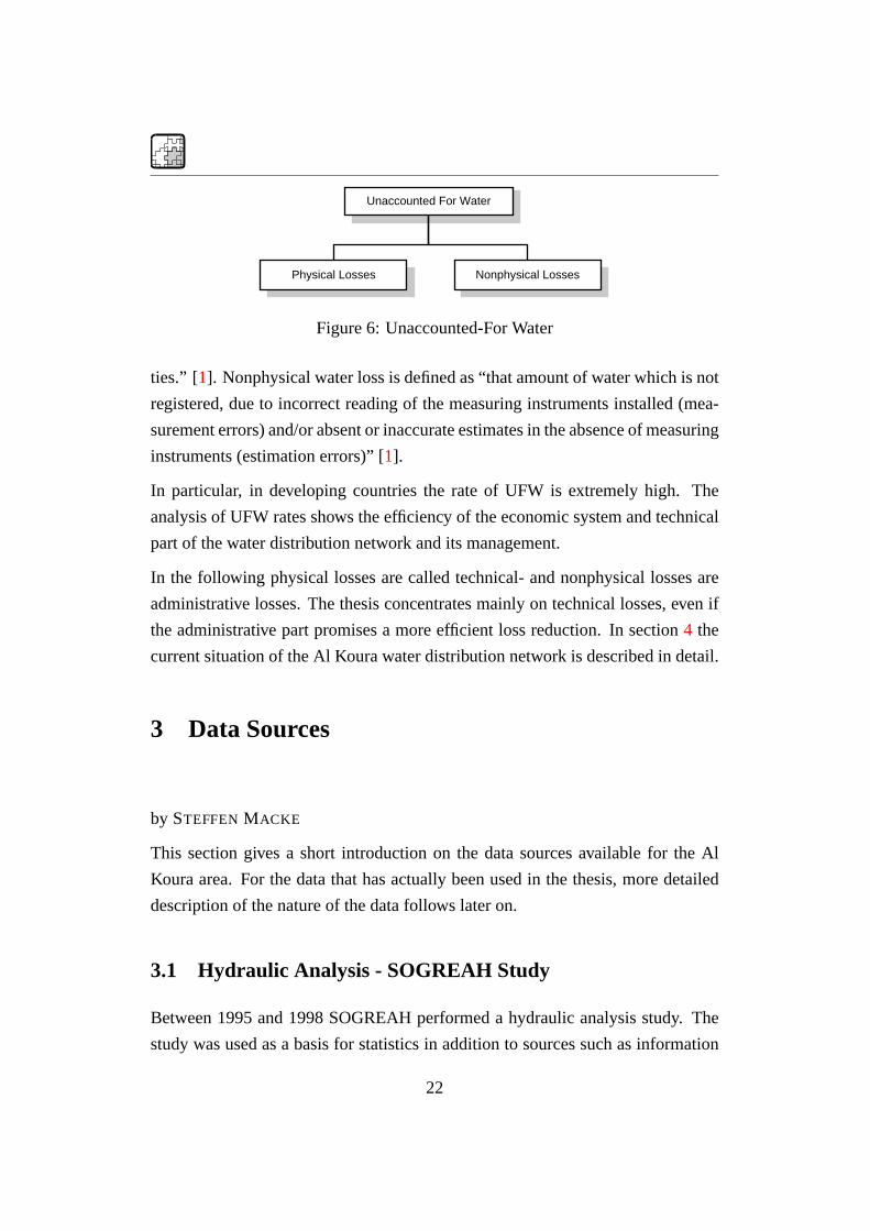
Unaccounted-for water is defined as the “Water loss calculated as the difference
between the quantity of water fed into a distribution system (drinking water pro-
duction) and the quantity of water put to legitimate use, which has been metered
or can be estimated. Quantities of water put to legitimate yet unmetered public
use, e.g. for fire fighting, or distribution system rinsing, have to be estimated.
Quantities of water that are wasted by the consumers or lost through leaking fit-
tings, as well as losses occurring between raw water extraction and input into the
distribution system are not considered as unaccounted-for water. Unaccounted-for
water includes both physical losses and nonphysical losses”[15] .
The term ’non-revenue water’ is frequently used. It describes the quantity of water
which is lost or withdrawn from the water network without being paid for.
Water Loss
Quantity priorDistribution
Quantity duringDistribution
Quantity afterDistribution
Figure 5: Water Loss
An international standardized definition of the term “water loss” does not exist
yet. In [15] it is suggested that “water loss and waste can be defined as the total
quantity of water that is lost or put to illegitimate use during the period of its
human utilization from the point of its extraction from a natural body of water [...]
to the point of its intended consumption.” In Germany water loss is fixed in the
national standard DIN 4046: “Water loss is that percentage of input that cannot
be accounted for by volume and is partially lost. It comprises both physical and
nonphysical losses.”
In Germany physical water loss are defined as “that amount of water which is
lost without being used due to failures and deficiencies in the distribution facili-
21
Unaccounted For Water
Physical Losses Nonphysical Losses
Figure 6: Unaccounted-For Water
ties.” [1]. Nonphysical water loss is defined as “that amount of water which is not
registered, due to incorrect reading of the measuring instruments installed (mea-
surement errors) and/or absent or inaccurate estimates in the absence of measuring
instruments (estimation errors)” [1].
In particular, in developing countries the rate of UFW is extremely high. The
analysis of UFW rates shows the efficiency of the economic system and technical
part of the water distribution network and its management.
In the following physical losses are called technical- and nonphysical losses are
administrative losses. The thesis concentrates mainly on technical losses, even if
the administrative part promises a more efficient loss reduction. In section4 the
current situation of the Al Koura water distribution network is described in detail.
3 Data Sources
by STEFFENMACKE
This section gives a short introduction on the data sources available for the Al
Koura area. For the data that has actually been used in the thesis, more detailed
description of the nature of the data follows later on.
3.1 Hydraulic Analysis - SOGREAH Study
Between 1995 and 1998 SOGREAH performed a hydraulic analysis study. The
study was used as a basis for statistics in addition to sources such as information
22

3.2 Comprehensive Subscribers Survey (CSS) Data
by the Department of Statistics and the annual reports of the governorates.
As the study is quite comprehensive, the report “Incorporating Water Loss Reduc-
tion Program” [11], which summarizes the results of the study has been used most
of the time.
The hydraulic simulation models accompanying the hydraulic analysis study do
not take intermittent supply into account - they are based on complete network
restructuring that do not require the intermittent supply of water any more. As an
example, the hydraulic simulation model for Judayta village consists only of the
DN 150 pipeline. Comparing such a model with the intermittent supply model
that is introduced later on would be pointless due to the different level of detail.
3.2 Comprehensive Subscribers Survey (CSS) Data
The Comprehensive Subscribers Survey that is currently being executed for the
whole Irbid Governorate is used to link base maps with customer information.
The link is established over a database field - primary key (PK) - that is shared
between the billing system (COBOSS) and the GIS. With the survey, the correct
primary key is assigned to each customer.
The process is also used to check base maps and customer data. Corrections are
done if necessary.
As the villages in the Al Koura district lack street names, the GIS primary key is
the only way to transparently locate customers.
3.3 COBOSS Data
The COBOL-programmed billing system used by WAJ is called COBOSS. In a
process of decentralization a new COBOSS system was recently established in
Irbid.
After completion of the CSS, the COBOSS data allows to integrate the actual
consumption data into hydraulic models as demand. The COBOSS data contains
domestic water meter readings for three-month periods.
23

3.4 DLS Data
COBOSS allows exporting the data as plain ASCII text files. These files can be
imported into the GIS or into spreadsheets for further analysis.
3.4 DLS Data
The Department of Lands & Survey (DLS)1 is the source for the base maps in
the GIS. These cadastral maps are also used in the Comprehensive Subscribers
Survey. The primary key used to link COBOSS and GIS is the same key that the
DLS is using.
The DLS cadastral maps are based on the Palestine Grid coordinate system, as
they build the base maps for the GIS, the GIS also uses the Palestine Grid coordi-
nate system. Table4 contains the parameters that describe the coordinate system.
Parameter Value
Projection CassiniReference Spheroid Clarke 1880
Reference Point 82 M, x=35 12 43.49, y=31 44 02.749False Easting 170251.55m
False Northing 126867.909mK 1
a (Semiminor Axis) 6378249.79me 0.082482165485
Table 4: Palestine Grid Coordinate System Parameters
3.5 RJGC Data
The Royal Jordanian Geographic Centre (RJGC)2 was the source for contour
maps.
One problem with the RJGC Data was that the RJGC uses a different coordinate
system, the Jordan Transverse Mercator (JTM). The transformation to the Pales-
tine Grid coordinate system was done with ESRI’s ArcInfo. The information in
[18] is useful to perform geographic coordinate system transformation.1http://www.dls.gov.jo2http://www.rjgc.gov.jo
24
3.6 Water Quality Data
3.6 Water Quality Data
Water quality data is currently recorded on a per-village basis, the exact location
is only known by the employee that is taking the sample. This way the records
become quickly, even though they are entered in a database.
A new ORACLE-based database system has been purchased. Hopefully, this will
ease the process of linking the available GIS data. That in turn could yield a
powerful analysis option, as the spatial distribution of contamination can only be
overlooked with the help of a geographic information system.
The Central Laboratories use EPANET V 1.00 to build hydraulic models for qual-
ity analysis. Intermittent supply is not taken into account by the models used, thus
the calibration of these models is doomed.
A knowledge transfer was hampered by time constraints and the Central Labora-
tories bureaucracy, requiring official letters.
3.7 Logging Campaign
The Logging Campaign took place from 13th to 15th January 2001 and covered
one full supply interval of Judayta village. In cooperation with the leak detection
of the Water Authority of Jordan (WAJ) flow and pressure measurements were
undertaken.
3.8 Altimeter Surveys
The main purpose of the altimeter surveys was to check the quality of the Digital
Elevation Models (DEM) created from the RJGC contour maps (section3.5).
3.9 Bucket Fill
A ’Bucket Fill’- test was used to assess the tank overflow of the Judayta pumping
station.
25

3.10 Air Release Valve at Customer Meters
3.10 Air Release Valve at Customer Meters
A simple water meter test setup including an air release valve was used to evaluate
water meter readings for intermittent supply.
3.11 Internet
Figures1 and2 use geographic data (shapefiles) that has been downloaded from
the web sites of ESRI3 and CDC4. The following web pages have been used as
entry points to obtain the data:
• http://www.cdc.gov/epiinfo/EIshape.htm
• http://www.esri.com/data/online/index.html
4 State of the Water Distribution Network Al Koura
by ARNE BATTERMANN
4.1 Overview
Currently the Al Koura water network consists of 210 km pipeline (DN > 50). The
major part of the network consists of galvanized iron (GI) pipes, 32% consist of
steel pipes (table5).
4.1.1 Pumping Stations
Two pumping stations are supplying Al Koura - the Judayta pumping station in the
south of the district and the Oyoun Al Hammam pumping station in the northern3http://www.esri.com4http://www.cdc.gov
26

4.1 Overview
part of Al Koura. These two stations are provided by two wells each. Each well is
equipped with a flow meter for a documentation of the well production. Figure7
shows Judayta pumping station.
Figure 7: Judayta pumping station
AppendixH gives an overview of the installations at Judayta pumping station.
Two additional booster stations are located in the outermost north and west of the
district. Two flow measurement locations are defined in the north and south for
documenting the flow out of the district for supplying direction Ajloun or Irbid.
AppendixI shall give an overview of the pumping and booster locations of pump
and booster stations, wells, water meters and the structure of the distribution net-
work. In spite of extreme elevation differences in the district, capacities of existing
reservoirs are not used and high-pressure zones exist in supplying zones.
For the Irbid Governorate the quantity of UFW is estimated with 55% on av-
erage. Administrative losses have a share of 60% and technical losses of 40%
27

4.2 Technical Water Losses
Pipe Length in km Percentage
Steel 66.867 31.8Galvanized Iron 118.271 56.1Unknown 24.640 11.8
Table 5: Pipe Materials in the Al Koura Distribution Network
on UFW[11]. Generally a discussion about influences on technical and adminis-
trative losses of water distribution systems is necessary in order to demonstrate
possibilities for improving the system.
In the following some influences on UFW in Al Koura are highlighted, which
have been observed during field visits.
4.2 Technical Water Losses
4.2.1 Bursts
A great part of the water network in Al Koura is lying uncovered on the ground
next to streets without any protection of demolition. It has been observed that
some pipes go through house walls and other pipes cross streets without any cov-
erage.
Judayta is a village, which is directly supplied by a pumping station 400 m below.
No surge protection is installed - water hammer is likely every time the supply is
stopped. This increases the danger of bursts (figure41).
4.2.2 Corrosion
The water network of Al Koura mainly consists of steel pipes (table5). Most of
them are lying on the ground and directly exposed to weathering.
4.2.3 Leakages
Leakages often result from inadequate repair of bursts. For example, refilling pipe
trenches with sand is no matter of course. It might happen that rocks of several
28

4.3 Influences on Administrative Water Losses
tons are used instead. The same applies for new parts of the network.
For the case that the pipe is covered, it is difficult to recognize leakages as the
sandstone that forms the terrain contains seams[2].
Leakages are caused by substandard fitting installations.
4.2.4 Zoning
In this report the water network of Judayta is analyzed. Zones are not clearly
separated and the existing zones are not operated in dependency to the hydraulic
optimum (section3.7).
Parts of the network are not well documented. ’Wild’ connections between supply
zones have been installed, without good or any documentation. Staff members,
knowing details about the complex network, are few. Within the scope of this
thesis 13.1% of pipes in Al Koura have been updated (table6).
4.2.5 Pressure
Pressures up to 41 bar have been documented during the logging campaign in Jan-
uary, 2001 (section3.7). Some domestic water meters have to resist pressures of
more than 30 bar over complete supply intervals. Currently, no pressure reduction
valves are installed.
4.3 Influences on Administrative Water Losses
In the following registered influences on nonphysical water losses (section2) are
discussed briefly.
Reduction of administrative losses goes further than improving measurement meth-
ods and procedures in direct connection to the water network. In many cases de-
ficiencies in administrative areas are responsible for a huge percentage of high
water losses.
29

4.3 Influences on Administrative Water Losses
4.3.1 Domestic Water Meter Inaccuracies
A number of the installed water meters do not reflect reliable measurements. Of-
ten this results in high pressures. Pressure reduction valves do not exist or are not
installed and the meters are not designed to face pressures up to 30 bar (section
3.7).
In section5.2 the effect of intermittent supply on domestic water meters is ana-
lyzed. Inaccuracies have to be confirmed. This survey is described and analyzed
in section5.2.
Frequently the water meters are manipulated by the subscribers. Statistics of the
time between January and October, 1999, published in [11] show, that in 70% of
illegal cases the water meters in the Al Koura area have been manipulated, in 20%
of the cases illegal connections have been installed in front of the meter. This
percentage refers to one illegal case out of 88 subscribers.
4.3.2 Bulk Water Meter Problems
• Damages due to of missing manholes are tolerated.
• It has been noticed that oversized or undersized meters have been installed.
• Flow directions in Al Koura vary with the supply of the different villages.
• Readings of the working meters at the well production are unreliable be-
cause they are estimated by the responsible operator.
4.3.3 Network Maintenance
According to reports by workers of the maintenance team bursts cannot be re-
paired or are repaired lately because of missing personnel.
4.3.4 Illegal Consumption
According to [11] the illegal connection cases in Irbid and Jerash are alarming.
Twenty-five percent of the subscribers are consuming water illegally. Even worse
30

is, that this percentage reflects the convicted cases only. The real percentage of
illegal water consumption might be even higher.
There is no prosecution of illegal water consumption. The reason might lay in the
public sector structure of the WAJ. A necessity of being economically does not
exist in the same way as on the private sector.
4.3.5 Objection Acceptance
Objections by customers on water bills are accepted by the responsible instances
of the water authority. Reasons might be missing responsibilities of the personnel
in the public water authority and a lack of interest.
According to statistics published in [11] 14.4% of the summarized objections of
the complete Irbid governorate are dismissed. In Al Koura only 12.9% are dis-
missed. This means that the majority of objections (nearly 90%) succeeded.
5 Surveys in Judayta
by ARNE BATTERMANN
In order to obtain reliable measurements, several surveys have been performed in
Judayta village and at Judayta pumping station. The following section shall give
an overview on these surveys. The importance of some particular problems will
also be discussed. Section5.1describes the bucket fill test at the well production
of Judayta pumping station. In section5.2 domestic water meters are tested on
accuracy under the influence of intermittent supply.
5.1 Bucket Fill
The pumping station of Judayta takes water from two wells (appendixH). These
wells are feeding a storage tank of app. 16m3. Each well is producing app. 80
31
5.1 Bucket Fill
m3
h . Normally only one well is running, while horizontal pumps take the water
from the tank to supply the villages. An automatic control for avoiding overflow
does not exist.
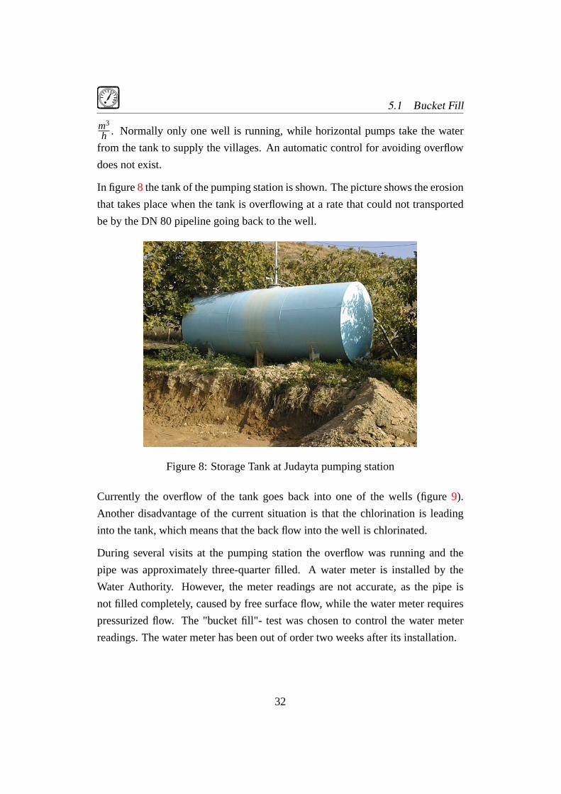
In figure8 the tank of the pumping station is shown. The picture shows the erosion
that takes place when the tank is overflowing at a rate that could not transported
be by the DN 80 pipeline going back to the well.
Figure 8: Storage Tank at Judayta pumping station
Currently the overflow of the tank goes back into one of the wells (figure9).
Another disadvantage of the current situation is that the chlorination is leading
into the tank, which means that the back flow into the well is chlorinated.
During several visits at the pumping station the overflow was running and the
pipe was approximately three-quarter filled. A water meter is installed by the
Water Authority. However, the meter readings are not accurate, as the pipe is
not filled completely, caused by free surface flow, while the water meter requires
pressurized flow. The "bucket fill"- test was chosen to control the water meter
readings. The water meter has been out of order two weeks after its installation.
32

5.1 Bucket Fill
ChlorinationTank
16 m^3
WellNo.1
WellNo.2
DN150W
W
WDN100
Overflow DN80
DN150
Kufr AbillJudaytaKufr Awan
Figure 9: Operation of Judayta pumping station
5.1.1 Realization
On 19th, January 2001 the water meter on the DN80 pipe from the tank to the
well has been taken off. Several tests of filling a bucket of 14 l at the opened pipe
(figure10) have been made and the time of filling has been recorded.
ChlorinationTank
16 m^3
WellNo.1
WellNo.2
DN150
Bucket Fill
W
W
WDN100
Overflow DN80
DN150
Kufr AbillJudaytaKufr Awan
Figure 10: Tank overflow measured by Bucket Fill.
Figure11 shows the bucket fill taking place. The bucket was the best that could
be found on site.
33

5.1 Bucket Fill
Figure 11: Bucket Fill Photo
5.1.2 Results
During all tests the bucket is filled in app. 4 seconds:
Q = 14l4s ·3600s
h = 12600lh = 12.6m3
h
At the time of the test, the water meter at the overflow showed a flow of 0.3m3
min:
Q = 0.3 m3
min ·60minh = 18m3
h
This means, that the water meter reading is wrong by 70 %.
Figure12shows a repair attempt of the water meter at Judayta well No.1.
5.1.3 Conclusion
At the time of these tests one well was working with a production of app. 90m3
h .
With taking the result of the bucket fill as average back flow, a percentage of 11%
of the produced water is running back into the well.
34

5.2 Air Release Valves at Customer Meters
Figure 12: Water Meter at Well No. 1
This means that the well efficiency is reduced by 10% at some times. The total
amount of back flow is hard to estimate with the current water meter setup at the
pumping station.
Meanings to solve the overflow problem are described in section9.2.
It is not possible to use the term unaccounted-for water in this case. In section2
is defined that “[...] losses occurring between raw water extraction and input into
the distribution system are not considered unaccounted-for water”.
5.2 Air Release Valves at Customer Meters
5.2.1 Background
With intermittent water supply, air is sucked and pushed in reliance with the status
of supply period because of empty running pipes. At the beginning of a supply
35

5.2 Air Release Valves at Customer Meters
period the air is pressed upward by the water filling the pipe and in the end of
the period air should be sucked as a consequence of empty running pipes. The
sucked air could turn back the domestic water meters and cause an enhancement
of unaccounted-for water.
5.2.2 Locations
Two locations were chosen for examining the reaction of the domestic water me-
ters on air in the network. Both locations (A and B) have an elevation of app. 270
m above pumping station (573 m aSL) shown in figure13. The domestic meters
have been tested over two supply cycles (two weekends).
�
�
Figure 13: Location of Domestic Meter Tests
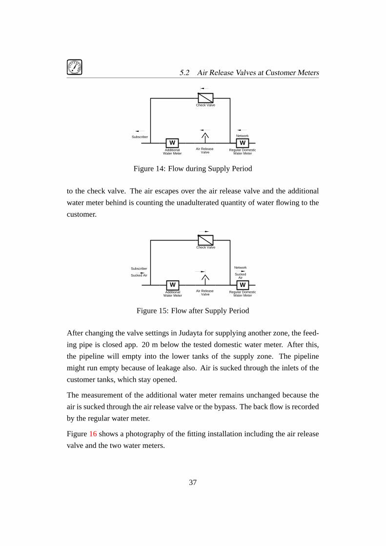
5.2.3 Realization
The installed arrangement consists of a check valve, an additional water meter and
an air release valve (figure14). The check valve is installed on a bypass parallel
to the regular pipe. The air release valve is fitted behind the domestic water meter
and another water meter is installed additionally behind the air release valve.
During the filling period water is flowing over the domestic water meter, which is
recording the billed quantity of water. During the supply the bypass is closed due
36
5.2 Air Release Valves at Customer Meters
W W NetworkSubscriber
Regular DomesticWater Meter
AdditionalWater Meter
Air Release Valve
Check Valve
Figure 14: Flow during Supply Period
to the check valve. The air escapes over the air release valve and the additional
water meter behind is counting the unadulterated quantity of water flowing to the
customer.
Subscriber
Sucked Air
W W
Check Valve
Regular DomesticWater Meter
AdditionalWater Meter
Air Release Valve
Network
SuckedAir
Figure 15: Flow after Supply Period
After changing the valve settings in Judayta for supplying another zone, the feed-
ing pipe is closed app. 20 m below the tested domestic water meter. After this,
the pipeline will empty into the lower tanks of the supply zone. The pipeline
might run empty because of leakage also. Air is sucked through the inlets of the
customer tanks, which stay opened.
The measurement of the additional water meter remains unchanged because the
air is sucked through the air release valve or the bypass. The back flow is recorded
by the regular water meter.
Figure16 shows a photography of the fitting installation including the air release
valve and the two water meters.
37

5.2 Air Release Valves at Customer Meters
Figure 16: Air Release Valve Installation
5.2.4 Results
The expected shortfalls in receipts can not be confirmed. Exactly the opposite
happens in three of four cases. Three times the additional water meter counted
less than the domestic water meter.
In Figure17 a difference between the billed and actual consumption of 11 - 16%
becomes obvious. This means that the billed consumption might be higher than
the actual consumption by the subscriber.
In Figure18 the difference between billed and actual consumption is not compa-
rable to the difference at location A, but the tendency exists during the first supply
interval. During the second interval the actual consumption is slightly higher than
the billed consumption.
38

5.2 Air Release Valves at Customer Meters
19.01.2001 12:00
20.01.2001 16:00
0
0,5
1
1,5
2
2,5
3
3,5
1nd Supply Intervall
Date of Measurement
Flo
w in
m3
26.01.2001 20:00
27.01.2001 08:00
0
0,5
1
1,5
2
2,5
3
3,52nd Supply Intervall
Billed Consumption
Actual Consumption
Figure 17: Result of Meter Test at Location A
19.01.2001 12:00
20.01.2001 16:00
4
4,1
4,2
4,3
4,4
4,5
4,6
4,7
4,8
4,9
1nd Supply Intervall
Date of Measurement
Flo
w in
m3
26.01.2001 20:00
27.01.2001 08:00
5
5,25
5,5
5,75
6
6,25
6,5
6,752nd Supply Intervall
Billed Consumption
Actual Consumption
Figure 18: Result of Meter Test at Location B
5.2.5 Conclusion
The span between the actual and billed consumption might depend on the location,
the behaviour of the consumer or sudden pressure drops.
Behaviour of Customer If all the consumers open their tanks before starting
the supply, the mistake by pushed air at the consumer on a high elevation is lower,
because the air escapes at the customers below also. This should be the actual
39
5.2 Air Release Valves at Customer Meters
situation because each customer is opening his tank in time to get as much water
as possible.
In case the customers below open their tanks lately the mistake at the subscribers
above is getting adequately bigger.
Location The mistake of sucked air should decrease with an increasing pressure
difference between closed valve and domestic water meter. If the water meter
is close to the valve which setting is changed for supplying another zone, the
connected pipe main is full of water for a longer time than at a higher house
connection, where back flow of air is happening soon.
Sudden Pressure Drops
• Sometimes the horizontal pumps in Judayta have to be stopped, because
the network pressure at the pumping station exceeds 40 bar. This causes a
pressure drop in the network and in connection with this a back flow of air
through opened household storage tank inlets at the consumers.
• Pipeline bursts can cause pressure drops.
In order to get an accurate analysis of the mistake of domestic water meters in ar-
eas suffering from intermittent supply, more tests are necessary. The dependencies
between location, customer’s behaviour, pressure drops, etc. are complex.
The survey results clearly show, that the quality of domestic water meter readings
in intermittent supply areas is limited even if the water meters are calibrated and
the personnel for the readings is reliable. For a better measurement of domestic
consumption, installations of air release valves are an opportunity.
However from the perspective of the water undertaking in this case accurate read-
ings are not desired for the following reasons:
• The air release valves are costly.
• They require additional supervision and maintenance.
40

• The recorded inaccuracy was in favor of the water undertaking. If the water
price is not covering the running costs, it is desirable to increase the water
price. In this case the misreading is increasing the water price - even though
this increase is not ’fair’ as it is not equally distributed.
6 Preparing a GIS for the Al Koura District
by ARNE BATTERMANN
This section describes the sequence of operations for building up a GIS for the Al
Koura district. Later on, the GIS data is used as source for hydraulic models in
EPANET. The necessary steps included:
• Collection of available digital water network data.
• Software choices.
• Creation of an appropriate database design.
• Conversion of the existing data to the database design.
• Update of the network data, based on paper sketches and field surveys.
• Quality Control.
• Documentation of data, database design and the preparation process.
6.1 Software
by STEFFENMACKE
Though the GIS software used should not be too important when creating a GIS,
a few words are necessary to line out the alternatives in this case. As DORSCH
Consult Amman and the Water Authority of Jordan use GIS software from ESRI,
it was natural to choose ESRI software.
41

6.1 Software
6.1.1 ArcInfo
ArcInfo is ESRI’s high end GIS system. The multitude of programs alone is
confusing:
ArcInfo Workstation The traditional command line oriented flavor of ArcInfo.
Useful mostly for GIS experts, as the command line appears very cryptic to end-
users.
ArcInfo Desktop A modern, Windows NT based version of ArcInfo.
The three core applications are:
• ArcCatalog, an application to preview and manage spatial data.
• ArcMap, map creation and editing software.
• ArcToolbox, a collection of spatial analysis and data conversion tools.
ArcInfo Desktop contains advanced concepts (Domains, Geometric Network) that
ease the quality control process. Though ArcInfo is not the target for GIS appli-
cations in Al Koura, it proofed to be very useful while checking the data. Some
ArcInfo concepts have influenced the database design.
6.1.2 ArcView
ArcView is also a powerful GIS software but targeted at the low-end market. As
there is a lot of functionality missing in ArcView, additional software packages, so
called ’Extensions’ are often required while working with ArcView. Nevertheless,
ArcView is suited for a lot of applications in the water utility sector.
42

6.2 Database Design
6.2 Database Design
The first step to establish a GIS is to create a database design. This becomes
clear with the current number of∼5400 records in the updated water distribution
network. Each record has several attributes (fields). As a consequence the number
of 5400 is increasing with a multiplier resulting from the amount of attributes.
Existing database designs for Amman and Taiz, Yemen lacked several required
features, some inconsistencies would have made it extremely complicated to ex-
tend these designs.
6.2.1 User Needs
by STEFFENMACKE
A water utility GIS typically targeted at several user groups:
• The operations staff (network maps, repair data, etc.).
• Accounting personnel (collection areas, assets management, etc.).
• Management (statistics and reports for decision support).
• Public (general information, file complaints over the internet).
Like the rest of the thesis, also the database design had to focus on the technical
part. Knowing that other user needs exist, special care has been taken to ensure a
well-documented and extensible database design.
6.2.2 Data Types
by STEFFENMACKE
GIS software as well as other databases allows the elaborate specification of data
types for the attribute fields. Nevertheless when it comes to converting data from
one format to another, the conversion process often imposes restraints on the data
43

6.2 Database Design
types used. This is especially true for the conversion process between an ArcInfo
geodatabase and ArcView’s default data format, the shapefile.
It was therefore practical to limit the number of data types used in the database
design to the following:
• spatial data types - represent spatial (GIS) data, so called shapes
– point - represents a point with x and y coordinates
– multi point - a collection of points that share their attributes
– polyline - a line with two or more vertices
– polygon - an area
• non-spatial data types
– integer - a number without floating point
– float - a number that contains a floating point
– string - a text
– date - a date
The actual names of these data types differ even between ArcView and ArcInfo -
these are the ones used in the thesis.
6.2.3 UML - Unified Modeling Language
by STEFFENMACKE
UML, the Unified Modeling Language is a standard developed by the Object Man-
agement Group (OMG). “The Unified Modeling Language (UML) is a language
for specifying, visualizing, constructing, and documenting the artifacts of soft-
ware systems, as well as for business modeling and other non-software systems.
The UML represents a collection of best engineering practices that have proven
successful in the modeling of large and complex systems.”[7] The OMG web site5
contains more information on UML.5http://www.omg.org
44

6.2 Database Design
Background UML has become an industry standard for CASE (Computed Aided
Software Engineering) tools. CASE tools allow structuring the often chaotic soft-
ware development process in a way that it becomes transparent. UML is well
suited for modern, object-oriented data models.
UML is quite complex, for example it defines the following diagrams:
• use case diagram
• class diagram
• behavior diagrams:
– statechart diagram
– activitiy diagram
– interaction diagrams:
∗ sequence diagram
∗ collaboration diagram
• implementation diagrams:
– component diagram
– deployment diagram
The database design for the Al Koura GIS as well as the data model for the DC
Water Design Extension (section7) only involved the class diagrams. The follow-
ing UML introduction will therefore focus on the class diagrams.
Benefits Independent of any programming language or other software involved
in the development process, UML allows to create standardized visual representa-
tions of data models. Such diagrams can serve as a discussion basis for developers
as well as non-developers involved in the design process.
45

6.2 Database Design
UML capable Applications A number of applications allow UML modeling,
Microsoft Visio is probably the most prominent one. Also Visio serves as a UML
CASE tool for ArcInfo.
For the present Al Koura GIS database design, dia6 was chosen as the UML ap-
plication. Being a free diagram creation software makes dia the first choice not
only for UML diagrams.
Like Visio, dia is very extensible. The file format used by dia is XML (eXtensible
Markup Language), an industry standard, that is very easy to convert to other file
formats.
During the project it was possible to show with proof-of-concept applications that
it is possible to load UML class diagrams created in dia to ArcView. Creating
SQL tables with such models is also easy. Hopefully these concepts will evolve
into practical solutions the future.
Class Diagrams Class diagrams are also known as “static state analysis dia-
grams” or “static structural diagrams”. The following will only describe class
diagrams composed of two elements: Classes and generalizations.
Classes describe objects with similar structure. In the diagram a class is repre-
sented by a three-compartment box, with the upper compartment containing the
class name. The middle compartment contains a description of the class attributes.
The lower compartment is used to describe the methods of a class. Methods are
not used in following; the class diagrams of the thesis will only contain classes
with empty lower compartments. In such cases the UML software usually allows
to switch off the lower compartment in order to create a visually more appealing
representation. However, in the following the third compartment is displayed in
order to be compliant with the UML standard.
Classes are separated into abstract and non-abstract classes. The difference be-
tween them is that abstract classes only exist in the UML model. Non-abstract
classes not only exist in the UML model but also in the data itself: They are visi-
ble as files or database tables, for example. To reflect the difference, the name of6http://www.lysator.liu.se/~alla/dia/
46
6.2 Database Design
abstract classes is displayed in italics in the diagram.
Generalizations are used to model the relationship between a more general ele-
ment (parent) and a more specific element (child). The child inherits all attributes
and methods from the parent.
In the diagram a generalization is represented by a line that stretches from the
parent to the child. The parent’s end of the line is marked by a large hollow
triangle.
XYPoint+x: float+y: float
ElevationPoint+elevation: float
WaterMeter+id: integer
ElevationPoint+x: float+y: float+elevation: float
WaterMeter+x: float+y: float+id: integer
(i) (ii)
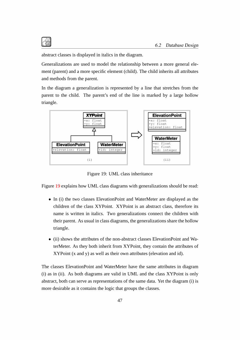
Figure 19: UML class inheritance
Figure19explains how UML class diagrams with generalizations should be read:
• In (i) the two classes ElevationPoint and WaterMeter are displayed as the
children of the class XYPoint. XYPoint is an abstract class, therefore its
name is written in italics. Two generalizations connect the children with
their parent. As usual in class diagrams, the generalizations share the hollow
triangle.
• (ii) shows the attributes of the non-abstract classes ElevationPoint and Wa-
terMeter. As they both inherit from XYPoint, they contain the attributes of
XYPoint (x and y) as well as their own attributes (elevation and id).
The classes ElevationPoint and WaterMeter have the same attributes in diagram
(i) as in (ii). As both diagrams are valid in UML and the class XYPoint is only
abstract, both can serve as representations of the same data. Yet the diagram (i) is
more desirable as it contains the logic that groups the classes.
47

6.2 Database Design
6.2.4 Implementation
AppendixE contains the structure of the database. Taking the pipes as an example,
the UML class diagram will be explained (figure20):
Together with the Node class the Pipe class shares the attributes of the Feature
class, which consists of 4 attributes. The superclass of the Feature Class is the
Identity Class. This class contains the most general element dc_ID. The attributes
of Identity are inherited by the classes Curve, Pattern and Feature. As a conse-
quence the Pipe class consists of 17 attributes like ’dc_ID’, for an identification of
each record, ’Installation_date’ for a documentation of age of the pipe or ’length’
for the length of the pipe.
Identity+dc_ID: string
Node+Shape: Point+Elevation: float+result_demand: float+result_head: float+result_pressure: float+ElevationSource: CodedValue
Valve+Diameter: integer+Type: string+Setting: string+Minorloss: float
Pipe+Shape: Polyline+Node1: string+Node2: string+length: float+diameter: integer+roughness: float+minorloss: float+status: string+Material: CodedValue+result_flow: float+result_velocity: float+result_headloss: float
Feature+Installation_date: date+Abandon_date: date+dcSubtype: CodedValue+BitcodeZone: integer
Pattern+multiplier: float
VirtualLine+result_flow: float+result_velocity: float+result_headloss: float
Curve+dc_x: float+dc_y: float
ElevationSource Values:0: Source Unknown1: 100 m Contours DEM2: SOGREAH Procedure Models3: Altimeter4: Paper maps5: estimated6: 25 m Contours DEM
Material Values:0: Steel1: Galvanized Iron2: PVC3: PE4: Ductile Cast Iron9: unknown
dcSubType Values:1: ShutOff Valve
Al Koura Bitcodes:0: Judayta
dcSubType Values:0: Network Pipe1: House Connection2: Leakage Tank Connection
Figure 20: Extract: UML Static State Analysis Diagram
In some cases notes are linked to the attributes of a class. These notes contain
domains and further define valid attribute values. They are implemented as coded
value domains in the GIS. The sense of these domains is to restrict the input into
a record to a defined input and to offer the opportunity to make queries for parts
of the network.
48

6.3 Quality Control
As an example the following pipe theme query will select only network pipes.
dcsubtype = 0
Similar to this example any kind of object of the water distribution network can
be selected by queries, with a database structure shown in appendixE.
Properties of attributes like different pipe materials under ’Material’ can be de-
fined as giving each kind of material a characteristic number.
In the same way the attributes of all other elements of the water network are de-
scribed in the diagram. The difference between pipes and the other elements is the
geometry of the class. While pipes are polylines all the other spatial classes (junc-
tions, tanks, pumps, valves and reservoirs) are points and therefore these feature
classes share the properties of the Node class.
6.3 Quality Control
One of the most important parts of GIS work is the quality control functionality.
A lot of time can be saved by using the quality-checking tools offered in GIS
packages like ArcInfo. Very often digital maps are going to and fro between GIS
operators and engineers. If the proper quality checks are missing in this process,
time and money are wasted.
The integration of quality control tools into the process of creating and updating
digital maps can yield many advantages for the company and the employees, such
as:
• Quality improvement of digital maps.
• Time savings for responsible engineers and with it savings in personnel
costs.
• Increase of motivation for everybody involved.
• Increase of delivered quality at the client and a resulting increase of esteem.
49

6.3 Quality Control
The integration of functions of ArcInfo into the sequence of operations in working
with the GIS is a single effort and might cost time and temper during establish-
ment. Nevertheless the results should justify this effort .
6.3.1 Domains
Domains have been used to ensure data quality.
Coded Value Domains These domains are limiting the inputs into a field of a
record to defined values. Pipe materials for example can be defined in a coded
value domain. Each material can be coded with a specific number as shown in
figure 20. After integration of a domain like this inputs, which are not equal to
one of the defined codes, are not accepted.
The advantage of limitations in the input into attributes of the database consists
of keeping the records clear. Spelling errors or impossible materials for example
can be excluded like this. Moreover the size of the database is decreasing because
number-fields are usually smaller than strings. As a consequence the database
is getting faster and does not require as much hard disc space as the equivalent
database without coded values.
Range Domains Are used for reducing the probability of entering values that
are out of a defined range. Also in this case an example can be found in the pipe
theme of the created database structure. For excluding mistakes by entering pipe
diameters a range is defined between 0 and 500. With a defined range like this it
is fixed that pipes below 0 and above 500 do not exist.
Because of the small leakage pipes the lower limit is defined with 0. Over validity
checks in ArcInfo all records of the database are selected automatically, which
violate the defined range domains.
50

6.4 Distribution Network Data Update
6.3.2 ArcInfo Geometric Network
In addition to domains other checks have been made for improving the quality
of the database. Often GIS maps have their source in CAD drawings. During
the digitizing work many mistakes may occur. It might happen that the snap-
ping functions are not focused correctly with the consequence of gaps between
elements that should be connected.
Missing intersections are very often the reason for quality loss. For digitizing a
connection of one pipe on another one of them has to be intersected, for creating
a new junction between the pipes. As mentioned this happens very often because
of wrong snapping.
Unnecessary intersections can reduce the quality of the map. Connectivity does
not exist anymore, if an intersection is set on a pipe without creating a new junc-
tion on this location. Plenty of these mistakes have been present in the network
which had to be updated in the scope of this thesis. The most important tool to
locate these mistakes has been the Geometric Network of ArcInfo. It allows to
check the connectivity of complex networks including pipes, junctions, valves,
pumps, tanks and reservoirs.
Connectivity With setting a so called “flag” at one element of the network
(junction, pipe, valve, etc.) a trace the can be started in the Geometric Network,
which selects all those elements that are connected with the flagged element. For
getting an accurate state of the network all selected elements should be marked
with a temporary attribute. After un-selecting the elements a query can be started
for all those elements, which have not been marked.
6.4 Distribution Network Data Update
The update contains new pipes of the network as well as functional parts like
valves, washouts, pumps, tanks, reservoirs, water meters, endcaps, etc. The update
includes quality checks for connectivity and automatic validity control of records
51

6.4 Distribution Network Data Update
in defined ranges. The continuous quality control is the key for a good network
update. The bulk of work consists of correcting digitizing mistakes.
The quality of the source material of the network has been poor. Zones have not
been clear because of missing valves and wrong connections of pipes. Pipes and
junctions have sometimes been double at the same location. Quality checks have
not been undertaken before handing over the data. Table6 gives an overview of
the quantity of elements added to the network. The table is not reflecting the work
connected with updating the network because a great part consists of changing
attributes of existing records without adding new records. This is not shown in
table6.
Elements of the Network State ofNovember’00
State ofFebruary’01
Percentageof Increase
Pipes DN25 in km 0 2.259 100Pipes DN50 in km 112.842 130.383 13.4Pipes DN75 in km 2.955 2.957 0.1Pipes DN100 in km 33.949 34.927 2.8Pipes DN125 in km 7.859 7.855 -0.1Pipes DN150 in km 8.863 12.501 29.1Pipes DN200 in km 15.789 18.779 15.9
total Pipes in % 182.256 209.616 13.1Number of Pumps 0 15Number of Valves 0 152
Number of Reservoirs 0 3Number of Washouts 0 3
Number of Water Meters 0 4Number of Endcaps 330 339Number of Tanks 0 1
Table 6: Network Data Update Statistics
With the process of correcting present data app. 13% of the network have been
updated. 27 km of pipeline are added and 152 valves are placed in the distribution
system. Pump and booster stations as well as the locations of wells are integrated
into the network. Reservoirs are integrated for the south of Al Koura. AppendixI
shows the updated water distribution network of Al Koura.
52
6.5 Check and Integration of Elevation Data
With handing over the water distribution network the quality checks described in
section6.3 have been passed successfully. The attributes adhere to the domains
and the network connectivity is established.
6.5 Check and Integration of Elevation Data
This section describes the steps of checking and integrating the elevations de-
livered as paper map by the RJGC. The paper maps are digitized and a digital
elevation model is build. Interpolation is the key for creating digital maps. The
mistake is de- and increasing with the accuracy of the source data. In this case
the source consists of 25m-contour paper maps. This means that the maximum
mistake can be 25m.
Spot heights are taken for making a cross-check with the delivered data. The spot
heights are taken with altimeters7, which are used differential to get accurate
readings. One stationary altimeter is used to correct the atmospheric pressure
variation over the time, while the second one is used in the field. The altimeters
have an accuracy of±5m, before using they are calibrated.
6.5.1 Data Check
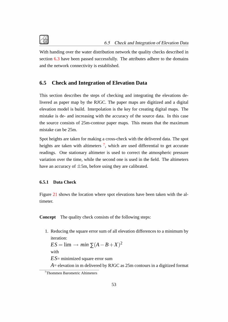
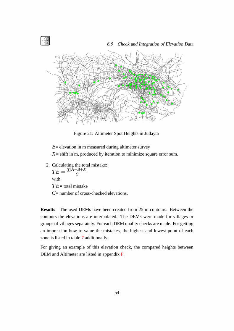
Figure21 shows the location where spot elevations have been taken with the al-
timeter.
Concept The quality check consists of the following steps:
1. Reducing the square error sum of all elevation differences to a minimum by
iteration:
ES= lim → min∑(A−B+X)2
with
ES= minimized square error sum
A= elevation in m delivered by RJGC as 25m contours in a digitized format7Thommen Barometric Altimeters
53
6.5 Check and Integration of Elevation Data
� ��
��
�
�
�
�
�
�
��
��� ��
�����
� ���
�
�
���
��
�
�
��
��
�
�
�
�
�
� ��
�
�
��
��
��
� � �
�
�
�
�
��
��
�
���
����
�
����
� �
�
��
�
�
�
�
�
�
�
�
Figure 21: Altimeter Spot Heights in Judayta
B= elevation in m measured during altimeter survey
X= shift in m, produced by iteration to minimize square error sum.
2. Calculating the total mistake:
TE = ∑|A−B+X|C
with
TE= total mistake
C= number of cross-checked elevations.
Results The used DEMs have been created from 25 m contours. Between the
contours the elevations are interpolated. The DEMs were made for villages or
groups of villages separately. For each DEM quality checks are made. For getting
an impression how to value the mistakes, the highest and lowest point of each
zone is listed in table7 additionally.
For giving an example of this elevation check, the compared heights between
DEM and Altimeter are listed in appendixF.
54

6.6 Visualization
Village HighestPoint mabove SL
LowestPoint mabove SL
ElevationDiffer-ence inm
Shiftin m
TotalMis-take in%
Judayta 713 302 411 22.93 12.92Kufr Awan,Kufr Abil
521 324 197 14.93 8.96
Table 7: Cross-Check of DEM with Spot-Heights
6.5.2 Integration into GIS
The integration of the checked DEM is done with the DC Conversion Extension.8
New records in a defined field of a chosen point theme are generated by using the
extension. In reliance on the coordinates of points the corresponding grid values
are added to the point theme. The elevations of Judayta, Kufr Awan and Kufr
Abil are updated. The contours of the centre and northern part of Al Koura have
not been bought as DEM yet and consists of elevations taken from a DEM that is
based on a 100 m contours.
No matter which area of Al Koura, each point of the point themes got an eleva-
tion. The source of elevation is documented for each record in the field ’Eleva-
tionSource‘ as illustrated in appendixC.
6.6 Visualization
by STEFFENMACKE
The hydraulic simulation of water distribution network is a complex task. For hilly
areas a discussion of such simulation models is only possible with the knowledge
of the topography.
Modern information technology allows visualizing digital elevation models in real
time.
Such Visualization tools are the ideal companions to powerful network analysis8The DC Conversion Extension is Development of DORSCH in ArcView, ESRI
55

software - the integration of hydraulic modeling software into the GIS will even
allow the integration of network analysis and three-dimensional visualization.
The GIS created for Al Koura contains the data to create three-dimensional vi-
sualizations. Without further processing, however, the resulting representations,
called scenes, will look odd.
An appealing 3D-Visualization requires several steps:
• Interpolate the DEM to a level that was unnecessary for the hydraulic cal-
culation. The accuracy that is accomplished by this operation is virtual - the
model is displayed smoother because of this. The observer’s eye recognizes
less raster patterns in the output.
• Densify the pipelines: In simple words, the pipes had to be split in segments
of 1 m length in order to get best display results.
• Draping the DEM with an aerial photograph makes the visualization look
more realistic.
Three-dimensional visualizations have been used in the project to check the DEMs.
7 Modeling Intermittent Supply using EPANET and
ArcView
by STEFFENMACKE
The EPANET hydraulic engine is very powerful. However, a ’normal’ EPANET
model is not suited for intermittent supply analysis. Several steps are necessary to
overcome this problem. These steps heavily depend on data preparation with GIS
software like ArcView.
The following section will summarize the concepts used to establish an intermit-
tent supply capable hydraulic model using ArcView and EPANET software.
56

7.1 ArcView Extensions
It will also be an introduction to a software module developed during this project
that allows the integration of EPANET hydraulic models in GIS data.
The motivation to create such software even though there are software packages
available that provide a lot of the necessary functionality is clearly financial:
ArcView is a low end GIS software package, the high end ArcInfo software comes
with network trace functionality and connectivity checks but constrains the user
to proprietary data model. The proprietary data model in combination with the
high price (approximately tenfold the price of ArcView) were the reasons not to
use ArcInfo (section6.1).
After careful consideration, the GNU Lesser General Public License (LGPL) was
chosen for the software described hereafter[9]. DORSCH Consult decided to
make the software available for free on the internet9.
The GNU Lesser General License is an open-source license that enables every-
body to develop the software further - if the developer agrees in turn to license
and publish his additions under the LGPL.
7.1 ArcView Extensions
ArcView GIS software provides a powerful way to extend the software’s capabil-
ities: So called ’Extensions’ written in ArcView’s scripting language AVENUE
that seamlessly integrate with ArcView’s graphical user interface. ArcView Ex-
tensions are typically installed and removed very easily. The user decides which
extension to load during the ArcView session - depending on the problems he
wants to analyze. The software module developed is called “DC Water Design
Extension” and consists of approximately 6000 lines of AVENUE source code.
AppendixA contains the DC Water Design Extension Manual. AppendixB con-
tains the description of the Data Model used by the DC Water Design Exten-
sion. In order to model more complex systems, reading the EPANET 2 Users
Manual[16] is recommended.9http://dcwaterdesign.sourceforge.net
57

7.2 Substitution of Demand Nodes with Small Tanks
7.2 Substitution of Demand Nodes with Small Tanks
Intermittent supply yields a fundamentally different demand pattern than continu-
ous supply. In fact, there is no demand pattern: The storage tanks of the customers
will fill up whenever the systems provides water, until they are full and the float
valve closes[19].
The approach to substitute demand nodes with small tanks in intermittent supply
models has been used once in a thesis in Palestine. However it was not possible
to get hands on the respective paper.
The software described in [19] utilizes 4 components to model intermittent water
supply:
• Demand Model
• Secondary Network Model
• Network Charging Model
• Modified Network Analysis Method
While this approach is far more sophisticated and may provide superior results, it
requires more specialized software. The substitution of demands with generalized
tanks makes it possible to model pressure dependent demand transparently with a
number of existing hydraulic network analysis software packages and is therefore
very flexible.
7.2.1 Tank Sizes
The tank sizes depend on whether the network is available down to the individual
house connection level or not. If the individual house connections are available in
a GIS, each tank in the model should represent one real household storage tank.
In case the house connections are not available in the GIS, generalized house
connections should be generated. It is practical to create one tank per junction,
58
7.3 Pressure Dependencies
which is located at the centroid of the customers that are assigned to it. The one-
tank-one-junction relationship resembles the traditional nodal demand of junc-
tions. Additional a ’house connection’ pipeline has to be generated that connects
the tank with the junction.
7.2.2 Fill Rates
The individual tank fill rates depend mainly on the headloss over the pipeline that
connects the tank to the network. For the case that uses generalized tanks it might
be necessary to graduate the diameter of the connecting pipeline depending on the
size of the tank.
7.3 Pressure Dependencies
The intermittent supply model relies on pressure dependencies in two points:
• The customer demands are pressure-dependent because of their storage tanks.
• Leakage is pressure-dependent.
The substitution of demand nodes with tanks also enforces a pressure-dependency
for the customer demands.
7.3.1 Leakage
Leakage is pressure dependent. Especially if the water is supplied intermittent: In
times where the system is empty, there will be no leakage at all.
In traditional hydraulic models, leakage is equally distributed with the demand,
in general as a factor that increases all demands. (Assuming that there is a lot of
leakage where is a lot of consumption.) However, this assumption might not be
true for all water networks. A more flexible implementation of leakage is therefore
desirable.
59

7.3 Pressure Dependencies
Orifice Diameter
discharge rate inlm
= 0.9· (ori f ice diameter in mm)2 (1)
Equation1 has been found through regression from data available in [14].
Pressure Dependency The following equation describes the discharge through
an orifice[13]:
qi = Ki · (pi − po)β (2)
where pi is the pressure upstream of the orifice,pothe pressure downstream of
the orifice andβa value of 0.5 according to theory and laboratory experience.
Kistands for the orifice coefficient, which is orifice-dependent. The following
parameters also origin from [13]:
• po = 0 Leakage is discharge into the atmosphere.
• β > 1.18 Leakage defects are different than simple orifices. They are de-
formed by the network pressure.
Implementation Pressure-dependent leakage can be implemented with tanks
connected to the network with short pipelines of a very small diameter. Such
a setup creates flows that are similar to the discharge into atmosphere. Unlike
the tanks used to model the household storage tanks, the tanks used in leakage
modeling should never fill up completely - the leakage should only be limited by
the headloss over the connecting pipe.
As for the tanks used in demand modeling, EPANET ensures pressure-dependency
in this case. The parameterβ of equation2 can not be taken into account, but the
results should still be better than those of the traditional network model.
Unfortunately, no literature could be found on the relationship between diameter
and average leakage rates per metre of pipeline. The number of defects increases
60

7.4 Virtual Lines
for lower diameters[13], but the number of defects is not necessarily related to the
leakage rates.
Section8.3.5describes two approaches to overcome this problem.
7.4 Virtual Lines
In the EPANET hydraulic model, pumps and valves are represented as lines. From
the hydraulic modeling point of view this makes sense, as the orientation of the
valves and pumps is important information. In GIS data, pumps and valves are
typically represented as points, as they are also symbolized with point symbols.
Point data is lacking the orientation information. Because of the pipe-node duality
pipes and valves will be referred to as virtual lines in this section.
The pipe-node duality complicates the creation of hydraulic models from the GIS
data. It is possible to overcome the problem with one of the following solutions:
• Storage of orientation information for each virtual line in the GIS
• Take over the orientation of connected pipes
The second possibility has some advantages, as it does not require additional data
storage - it was applied in the described application. However, it imposes some
restraints on the data. The concept to model virtual lines as points in the GIS can
be summarized as follows:
• Each virtual line needs to have exactly two pipes connected
• Both connected pipes must be oriented in the same way: One pipe has to
start at the virtual line and the other pipe has to end at the virtual line
Figure22shows examples of different pipe orientations at a virtual line. The case
a shows a pump with two pipes connected that are oriented in the same way. This
allows the creation of the hydraulic model and is therefore considered valid. Case
b shows pumps with pipes connected that are not oriented in the same way. This
61

7.4 Virtual Lines
a b c
Figure 22: Virtual Line Validity
is invalid as is does not allow the creation of the hydraulic model. Case c is invalid
because the pump has more than 3 pipes connected to it. Note that the orientation
information of the pump symbol is not necessarily contained in the GIS data.
GISData
Pump
J1 J2
PJ1 PJ2
EPANET
J1 J2
Figure 23: Virtual Line Creation
Figure23depicts the conversion process of virtual lines:
1. Number and orientation of the pipes connected to the virtual line are checked
for validity
2. The virtual node is replaced with a junction (PJ1).
3. An additional junction is added (PJ2).
4. The pipe from the virtual line to the next node starts at the additional junc-
tion. ( PJ2 -> J2).
5. The pump or valve is created. It connects the two new Junctions (PJ1->PJ2).
62

7.5 Bit codes
The DC Water Design Extension follows this conversion process when it is creat-
ing EPANET models. Additional considerations used in the process are:
• The length of the virtual line is one metre.
• If the pipe starting at the virtual line is shorter than one metre, the virtual
line length is set to half of the pipe length.
7.5 Bit codes
Bit codes make it possible to store fields of yes-no information in ’normal’ num-
bers. Every bit in the number having the value 1 is considered set, every bit of
value 0 is not set. Thus making it possible to bit-code several independent pieces
of information in one ArcView Number.
As ArcView is using 32-bit (integer) numbers, it should be theoretically possible
to store up to 32 pieces of information. This requires that the databases where the
data is stored use 32-bit numbers as well. Tests up to 19 sets of yes-no have been
successful.
The following example shows how this concept allows storing the network infor-
mation in one seamless data set and utilizing the same network features in different
hydraulic models:
In figure24 the nodes of three hydraulic models are bit-coded for storage in the
GIS. Each zone has its own bit in the bit code, indicating if the node is used in the
model or not.
The DC Water Design Extension Manual (appendixA) contains more information
bit codes. The DC Water Design Extension provides some functions to work with
such bit codes.
7.6 Calibration
The calibration of the intermittent supply model for Judayta village was influenced
by a multitude of different factors.
63

7.6 Calibration
Zone 1
Zone 2
Zone 3
111
111111
111 111 110
110
001 010
100
0 00
Bit 1, Zone 1
Bit 2, Zone 2
Bit 3, Zone 3
110
Figure 24: Bit-coding Supply Zones
MeasuringError
Roughness
Leakage Consumption
Calibration
ModelLimitations
Figure 25: Calibration Influences
Figure25shows the influences that have been taken into account.
The following global parameters have been chosen to calibrate the intermittent
supply model:
• A factor to adjust the diameters of the leakage pipes
• The pipe roughness
64

7.6 Calibration
• A factor to adjust the diameters of the house connections
• A factor to adjust the sizes of the household storage tanks
• Three thresholds to distribute the size of the house connections
• A factor to adjust the pump power
This differs from the calibration of a traditional hydraulic model, where only one
global factor, the roughness is taken into account.
Though the Windows version of EPANET provides functionality to assess the
quality of a calibration, this was not enough to evaluate the multitude of possible
parameter combinations.
7.6.1 Genetic Algorithms
Genetic Algorithms are a method to optimize non-linear problems efficiently. For
this reason they have become popular with hydraulic analysis and water supply
network design software [17, 19]. Genetic Algorithms are based on a process
that is similar to the natural evolution: Individuals, which are more ’fit’ to solve
problems are more likely to be reproduced than other, not so fit individuals. The
resulting selection process speeds up the problem solution. The approach itself is
very generic, it is suited for many applications.
As the whole concepts stems from biology, the terms used to describe it are also
biological:
• Population
• Gene
• Allele
• Reproduction
• Mutation
65

7.6 Calibration
• Crossover
For the calibration, a gene is a set of parameters that describes one calibrated
model. An allele is one of the parameters. A number of genes, called population,
reproduces itself to form the next generation of genes.
As the parameters used in the calibration are not discrete, a concept is needed that
allows genes with alleles that cover the whole space of possible solutions. For
example it would be possible to create a population that is large enough to cover
the necessary solutions. However, this would reduce the process to a simple trial-
and-error one, as fitness evaluation and reproduction would only take place after
the results for the large population have been calculated.
Another concept to increase the diversity of the population are mutations: Muta-
tions allow changing the allele values of a gene. It has proved successful to allow
complete mutations of an allele as well as only slight alterations of a value.
75% 10% 10% 5%
valueunchanged
10%decrease
10%increase
randomvalue
Probability
original allele value
valuechange
?
Figure 26: Allele Mutation
Figure26shows the allele mutation probabilities that have been used in the genetic
program.
Diversity is also increased by the reproduction process itself: The two parents
(genes) of a child mix their alleles in a crossover process.
Figure 27 displays the reproduction process. The crossover point is chosen at
random.
66
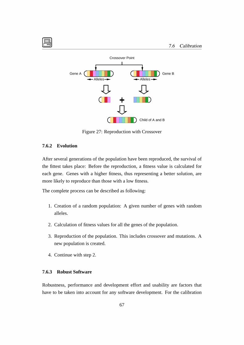
7.6 Calibration
Gene A Gene B
Crossover Point
Child of A and B
Alleles Alleles
+
Figure 27: Reproduction with Crossover
7.6.2 Evolution
After several generations of the population have been reproduced, the survival of
the fittest takes place: Before the reproduction, a fitness value is calculated for
each gene. Genes with a higher fitness, thus representing a better solution, are
more likely to reproduce than those with a low fitness.
The complete process can be described as following:
1. Creation of a random population: A given number of genes with random
alleles.
2. Calculation of fitness values for all the genes of the population.
3. Reproduction of the population. This includes crossover and mutations. A
new population is created.
4. Continue with step 2.
7.6.3 Robust Software
Robustness, performance and development effort and usability are factors that
have to be taken into account for any software development. For the calibration
67
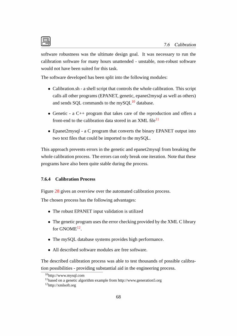
7.6 Calibration
software robustness was the ultimate design goal. It was necessary to run the
calibration software for many hours unattended - unstable, non-robust software
would not have been suited for this task.
The software developed has been split into the following modules:
• Calibration.sh - a shell script that controls the whole calibration. This script
calls all other programs (EPANET, genetic, epanet2mysql as well as others)
and sends SQL commands to the mySQL10 database.
• Genetic - a C++ program that takes care of the reproduction and offers a
front-end to the calibration data stored in an XML file11
• Epanet2mysql - a C program that converts the binary EPANET output into
two text files that could be imported to the mySQL.
This approach prevents errors in the genetic and epanet2mysql from breaking the
whole calibration process. The errors can only break one iteration. Note that these
programs have also been quite stable during the process.
7.6.4 Calibration Process
Figure28gives an overview over the automated calibration process.
The chosen process has the following advantages:
• The robust EPANET input validation is utilized
• The genetic program uses the error checking provided by the XML C library
for GNOME12.
• The mySQL database systems provides high performance.
• All described software modules are free software.
The described calibration process was able to test thousands of possible calibra-
tion possibilities - providing substantial aid in the engineering process.10http://www.mysql.com11based on a genetic algorithm example from http://www.generation5.org12http://xmlsoft.org
68
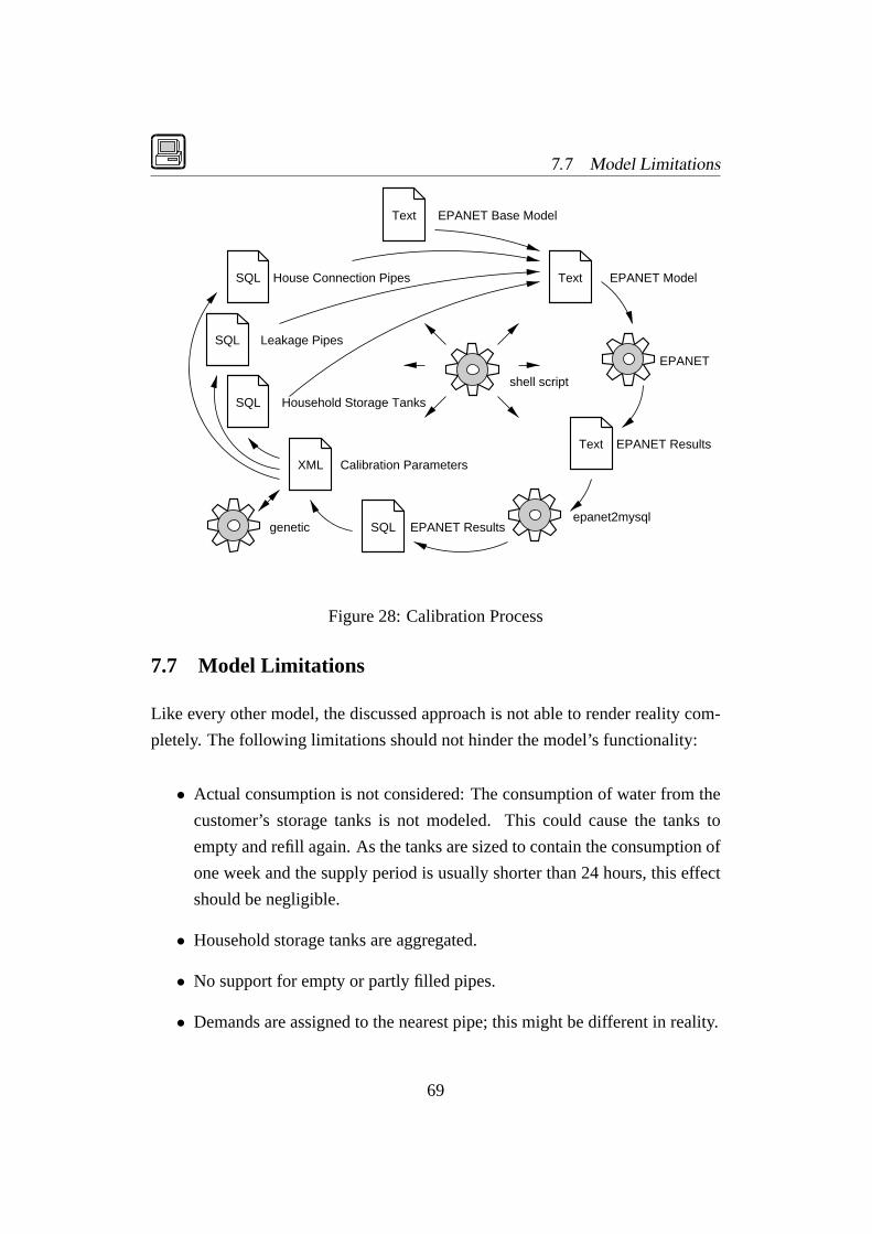
7.7 Model Limitations
XML Calibration Parameters
EPANET
Text EPANET Model
EPANET Base ModelText
SQL Household Storage Tanks
SQL Leakage Pipes
SQL House Connection Pipes
epanet2mysqlgenetic
shell script
SQL EPANET Results
Text EPANET Results
Figure 28: Calibration Process
7.7 Model Limitations
Like every other model, the discussed approach is not able to render reality com-
pletely. The following limitations should not hinder the model’s functionality:
• Actual consumption is not considered: The consumption of water from the
customer’s storage tanks is not modeled. This could cause the tanks to
empty and refill again. As the tanks are sized to contain the consumption of
one week and the supply period is usually shorter than 24 hours, this effect
should be negligible.
• Household storage tanks are aggregated.
• No support for empty or partly filled pipes.
• Demands are assigned to the nearest pipe; this might be different in reality.
69

• The consideration of unequal spatial distribution of leakage requires addi-
tional processing.
In addition, the model limitations for EPANET apply, see [16] for a discussion of
the limitations.
8 Intermittent Supply Model for Judayta
by ARNE BATTERMANN
This section describes the processes listed below:
• Definition of zones.
• Model creation.
• Logging campaign.
• Calibration.
Section8.3 is based on GIS operations described in section6. This section shall
describe the way to generate a running EPANET Model.
8.1 Definition of Zones
The zoning of the distribution system Judayta changes from summer to winter
time. While Judayta is divided into six zones from April to November (figure29),
the network is operated with four zones in the winter months shown in figure30.
The different zonings in summer and winter should allow an adjustment to differ-
ent demand patterns. In fact, the bigger winter zones reduce the pumping head a
little bit - higher friction losses are the reason.
During summertime each of the zones 2, 3, 4, 5 and 6 are supplied over 12 hours.
Zone 1 is supplied over the whole interval. Missing separation of zones is recog-
nizable between zone 5 and 6. Hazy zones are hatched yellow and brown. The
total duration of supply is 60 hours.
70
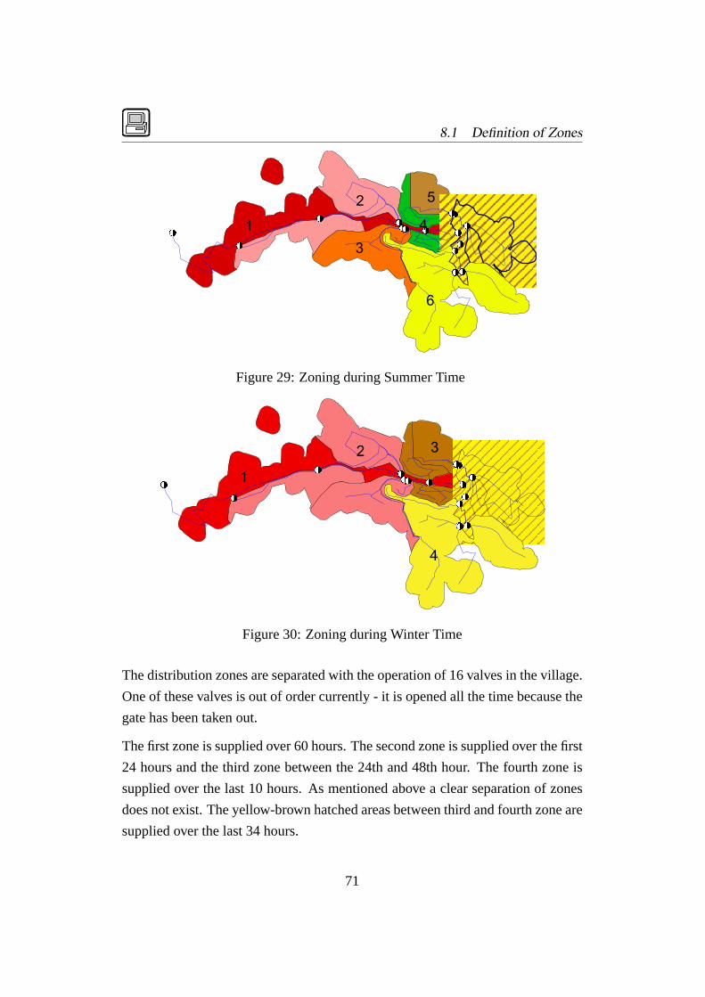
8.1 Definition of Zones
� �
� �
� �� �
� �
� �� �� �
� �� �
� �
� �
� �� � � �
� �
� �
Figure 29: Zoning during Summer Time
� �
� �
� �� �
� �
� �� � � �
� �� �
� �
� �
� �� � � �
� �
� �
Figure 30: Zoning during Winter Time
The distribution zones are separated with the operation of 16 valves in the village.
One of these valves is out of order currently - it is opened all the time because the
gate has been taken out.
The first zone is supplied over 60 hours. The second zone is supplied over the first
24 hours and the third zone between the 24th and 48th hour. The fourth zone is
supplied over the last 10 hours. As mentioned above a clear separation of zones
does not exist. The yellow-brown hatched areas between third and fourth zone are
supplied over the last 34 hours.
71

8.2 Domestic Consumption
This schedule may vary depending on necessities. During the logging campaign
the scheduled timetable was basically valid.
8.2 Domestic Consumption
For the integration of the COBOSS data (section3.3) the data needs to be checked
(section8.2.1). Afterwards the consumption of subscribers in Judayta has to be
integrated into the GIS. The workflow is described in section8.2.2.
8.2.1 Data Check
The delivered COBOSS data consists of 4 meter-reading cycles from January
2000 to October 2000. Two of the cycles represent winter consumption and the
other two cycles the summer consumption. In table8 the billed consumption of
Judayta village cycle is shown for the mentioned reading cycles.
Judayta has 1212 registered subscribers. In [11] based on the hydraulic analysis
study of SOGREAH (Chapter3.1) 8.5 persons are assigned to one subscriber in
the greater area around Irbid.
Consumption January 2000 April 2000 July 2000 October 2000
in m3
QuarterYear 40141 33537 37623 49140
in m3
w 2867 2395 2687 3510
Average inm3
w 2541
in lc·w 278 247 341
in lsubscr·d 338 308 414
in lc·d 40 35 49
Table 8: COBOSS Data Summary
The values for the consumption worked out in table8 are within the ranges in
Irbid of 180 - 650 lsubscr·dand a resulting per capita consumption of 22 - 76
lc·dpublished in [11].
72

8.2 Domestic Consumption
With a measured well production of app. 80m3
h and an estimated back flow of 10%
(chapter3.9) at the well production an estimated average quantity of app. 70m3
h is
pumped to Judayta over 60 hours of supply:
Quantity of water pumped to Judayta during one full supply period (logging cam-
paign / winter 2001):
70m3
h ·60h = 4200m3
Difference between pumped quantity and average billed consumption during win-
ter months in Judayta :
4200m3−2542m3 = 1658m3
1658m3
4200m3 ·100= 39.5%
The result is an UFW figure of app. 40%. This result reflects the expected value
according to the tendency of decreasing UFW during the last ten years in Irbid
and Jerash Governorate [11].
8.2.2 GIS Integration
In order to integrate the COBOSS data into the hydraulic model a sequence of
operations has to take place.
• Import of ASCII data into the GIS.
• Creation of points for each specific consumption.
• Generalization: Creation of tanks with conformist size and spatial relation
to the subscribers.
• Connection of tanks and water distribution network.
Tabular and Spatial Data The link between the tabulated COBOSS and the
GIS data is the primary key (PK) as used by the DLS. The PK is a unique ID for
every single parcel in Jordan. Before the two data source can actually be linked,
the following clean-up process has to take place:
73

8.2 Domestic Consumption
The spatial data may contain duplicate primary keys for some reasons. For ex-
ample, if a house is shown on the parcel, house and parcel will be represented by
two records in the database, sharing the same PK. In order to prevent the billed
consumption from being duplicated, all GIS records sharing the same PK have to
be merged into one record.
There are also duplicated primary keys in the COBOSS data. Every time a parcel
is home to more than one subscriber such duplications happen. As for the GIS
data, it is necessary to merge all records sharing one PK into one. Additional,
the billed consumption has to be summarized in order not to get lost during the
linking process.
The steps required for joining COBOSS and GIS data are shown in figure31.
After summary of equal PKs and concurrent creation of total consumption for
each primary key the tabular and spatial data can be joined based on the PK. Now
the spatial records in the GIS are completed with the characteristic consumption
and the next operation in the sequence for integrating the consumption into the
hydraulic model can start.
Join Tabular andSpatial Databased on PK
SummarizeConsumptionfor each PK
Dissolve Featuresof
equal PK
Figure 31: Join of Tabular and Spatial Data
74

8.2 Domestic Consumption
The ArcView functions used have been particularly the ’Summarize’ function for
the tabular data and the ’Geoprocessing Wizard - Dissolve features based on an
attribute’ for the spatial data.
Consumer Parcel Selection As only the parcels with actual consumption are of
interest, these are selected with a query. The following steps will only use these
consumer parcels.
Parcel Centre Points Within the next operation shown in figure32, points shall
be created, which contain the specific consumption of its polygons and the at-
tributes of the nearest junction. Afterwards points are created in the centre of each
polygon.
These points locate the house tanks. Therefore each centre point has to have the
information to which junction of the water network it shall be connected, because
house connections will be created between the tanks and the nearest junctions.
By joining the attributes of the nearest junction with the consumption in the new
generated centre points each centre point has the ID of that Junction and a relation
is created.
CreateSubscriber Polygon
Centre Points
Join Attributes of Centre Pointsand Junctions
Cut offSubscriberPolygons
Figure 32: Centre Point Creation
In this operation the ’DC Conversion Extension’ and the ’Geoprocessing Wizard
are used. Centre points are created over ’DC Conversion Extension’13, while the
’Geoprocessing Wizard - Spatial Join’ function is used to join the attributes of
junctions with the attributes of the nearest centre points.13A small ArcView Extension developed by DORSCH Consult
75
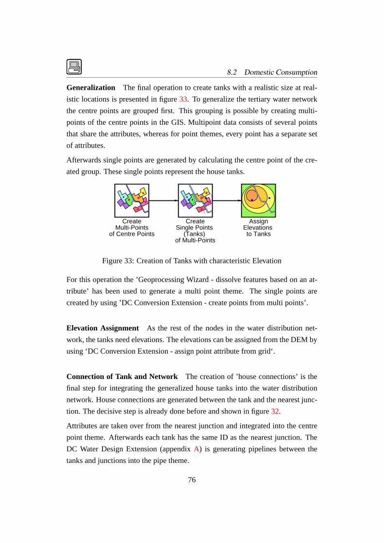
8.2 Domestic Consumption
Generalization The final operation to create tanks with a realistic size at real-
istic locations is presented in figure33. To generalize the tertiary water network
the centre points are grouped first. This grouping is possible by creating multi-
points of the centre points in the GIS. Multipoint data consists of several points
that share the attributes, whereas for point themes, every point has a separate set
of attributes.
Afterwards single points are generated by calculating the centre point of the cre-
ated group. These single points represent the house tanks.
CreateMulti-Points
of Centre Points
CreateSingle Points
(Tanks) of Multi-Points
AssignElevations to Tanks
Figure 33: Creation of Tanks with characteristic Elevation
For this operation the ’Geoprocessing Wizard - dissolve features based on an at-
tribute’ has been used to generate a multi point theme. The single points are
created by using ’DC Conversion Extension - create points from multi points’.
Elevation Assignment As the rest of the nodes in the water distribution net-
work, the tanks need elevations. The elevations can be assigned from the DEM by
using ‘DC Conversion Extension - assign point attribute from grid‘.
Connection of Tank and Network The creation of ’house connections’ is the
final step for integrating the generalized house tanks into the water distribution
network. House connections are generated between the tank and the nearest junc-
tion. The decisive step is already done before and shown in figure32.
Attributes are taken over from the nearest junction and integrated into the centre
point theme. Afterwards each tank has the same ID as the nearest junction. The
DC Water Design Extension (appendixA) is generating pipelines between the
tanks and junctions into the pipe theme.
76

8.3 Hydraulic Model Creation
The major part of the work in the GIS is done with the connection of tanks with
the distribution network.
8.3 Hydraulic Model Creation
In the present section the steps necessary to create a hydraulic model out of the
GIS. The Water Design Extension (appendixA) serves as the interface between
ArcView and EPANET several tables and rules (section8.3.6) have to be inte-
grated into the process of converting the GIS data into an EPANET import file.
Preparing a separated model of Judayta is described in section8.3.1. The elements
of the network are defined in section8.3.2. EPANET is a complex tool with
powerful capabilities, therefore adjustments have to be made for this particular
hydraulic model (section8.3.3). The integration of demand and leakage into the
model is explained in the sections8.3.4and8.3.5.
8.3.1 Isolation of Judayta
The isolation of Judayta in the GIS is necessary for creating an EPANET model
of this single village. The Water Design Extension provides a function that min-
imizes the work to cut out the elements belonging to one distribution zone like
Judayta. This function for cutting off so called bit-code zones is described in
section7.5.
Once the elements of the Judayta water network or any other village need to be
defined with an attribute in each theme. This attribute consists of a particular
value for each village of Al Koura (figure24). This means that the network of
each village can be cut out separately and elements that are shared with other
models (e.g. the pumping station) are included.
The aim of this method is to automate the process of manually cutting out the
villages after updating elements in the GIS (new pipes, new valves, etc.), while
still allowing to work on one seamless network map.
77
8.3 Hydraulic Model Creation
8.3.2 Elements of the Model
For creating an EPANET model of Judayta the following network elements are
necessary:
• Junctions
• Valves
• Pumps
• Tanks
• Reservoirs
• Pipes
The following paragraphs shall give an overview about the elements of the net-
work.
Junctions Junctions are connected by pipes. The demand of the junctions is set
on 0 because in this approach consumption is implemented with the tanks.
Valves Valves allow to define distribution zones in extended period simulations
(section8.3.6). Judayta consists of 16 valves. One of these valves is currently out
of order. All the network valves are modeled as Shut-Off-Valves (SOV).
Pumps The operating pump during supply of Judayta has to be characterized.
Important pump informations like power (sectionB.5) and pump curve (section
B.15) are integrated over the attributes “Power” and “Properties”. While power
is implemented as a value in the pump theme, the pump curve is integrated as an
extra table with x- and y-coordinates. The data in the ”properties”-field is a link
and contains the name of the pump curve.
78

8.3 Hydraulic Model Creation
Tanks Tanks are integrated to model leakage and demand. To different types of
tanks are used:
• House tanks.
• Leakage tanks.
The house tanks generated in section8.2.2 are reflecting the demand of those
subscribers, who are summarized in these tanks. Further explains for integrating
the demand into the hydraulic model can be found in section8.3.4.
The leakage tanks are generated at each junction of the water distribution net-
work. The limiting factor for leakage is not the tank size but the diameter of the
connection pipe (section8.3.5).
Reservoirs A reservoir is necessary at the pumping station to feed the pumps
in the EPANET model. It is a simplification of the hydraulic model. The two
wells, which are filling the storage tank in Judayta pumping station (figure9) are
not integrated in the hydraulic model. Instead a reservoir is chosen for supplying
the operating horizontal pumps. This reservoir resembles the pumping station’s
storage tank which is filled by the submersible pumps.
Pipes The pipes are structured in three types. The following types are defined:
• Network pipes.
• House connection pipes.
• Leakage tank pipes.
Network pipes represent the updated network of Judayta (section6.4).
The operations in the GIS for creating house connection pipes are shown in section
8.2.2. The house connection pipes shall supply the generalized house tanks. 125
house connections do exist in Judayta. It has to be made sure that a back flow of
79

8.3 Hydraulic Model Creation
water from the house tank (section8.3.4) is not possible. This has to be defined in
the pipes theme of the GIS (section8.3.6).
Leakage tank pipes are generated between the leakage tanks and the nearest junc-
tion. The GIS operations for generating these pipes are equal to the operations
for house connections (section8.2.2). The present hydraulic analysis model of
Judayta village features of 157 leakage pipes. Each pipe has a length of 2 metres.
The diameter of the leakage pipe is the key for modeling leakage in this approach.
8.3.3 Implementation of Model Adjustments
For running an EPANET model basic adjustments have to be fixed. They have to
be defined over the following items:
• Options
• Report
• Times
Options The options table allows to choose the used head-loss formula (in this
case Darcy-Weissbach), define flow units (litres per second). The number of trials
for finding hydraulic solutions can be specified (sectionB.11).
Report These adjustments are not of the priority like Options or Times. The
scale can be determined for getting different kind of summaries, status or warning
reports. The used adjustments are described in appendixB (sectionB.12).
Times The hydraulic time step and the duration of simulation period have to be
defined. The duration is set to 58 hours and a hydraulic time step of 5 minutes is
chosen.
Next to these to adjustments further items have to be defined (sectionB.13)
80

8.3 Hydraulic Model Creation
8.3.4 Modeling Demand
While classical models have a specified demand at each network junction, the de-
scribed approach is based on tanks which are filling in dependency of the present
pressure at the tank (section7.3).
The creation of house tanks is shown in section8.2.
For a better visualization of the development of pressure and demand in EPANET
each tank is reduced in its height to one metre. Like this a pressure scale from 0.1
to 1.0 in EPANET can visualize the tank fill level during the simulation period.
The tank volumes have to be converted. Each tank is of cylindrical shape with a
varying diameter and a constant height of one metre:
V =π ·d2
4·1.0 (3)
d =
√V ·4
π(4)
with
d = Tank diameter
V= Volume of tank established in section8.2.
The house tanks are supplied over the so-called “house connection pipes”. The
diameter of all the house connections was initially chosen with 25mm. This global
diameter yields a mistake because the diameters for house connections vary in
reality. To overcome the problem, the calibration script provides functionality to
graduate 4 diameters based on the size of the house tank. Such a model represents
the reality much better than a global diameter - it is still an error source, though.
To prevent a back flow of water out of the house tanks check valves are integrated
into the model. Each house connection pipe is equipped with a check valve as
shown in Figure34.
81

8.3 Hydraulic Model Creation
HouseTank
CVJunction
Figure 34: Check Valves
8.3.5 Modeling Leakage
For integrating the leakage into this approach of modeling intermittent supply,
tanks are created at each junction of the water distribution network. The rate of
leakage depends in this approach on the pipe length connected to the junction.
Two neighboured junctions are sharing the connected pipe with 50% of the length
each. The diameter of the leakage pipe should depend on the resulting pipe length
of the distribution network. Two approaches have been tried for integrating leak-
age into the model.
• Dependency between network pipe surface and leakage.
• Dependency between network pipe length and leakage.
The second approach seems more promising.
Repair statistics, published in [12], show that the majority (more than 90 %) of
the repairs have been done on pipes of DN50 and smaller. The network of house
connections is not integrated into the computed model and therefore this statis-
tic can not be reflected. This is not the case in the represented hydraulic model.
House connections are present, but they are unreal. Consumers are summarized
and the real total length of house connections behind a particular tank of the hy-
draulic model can be much bigger than defined by the length of the modeled house
connection.
l = l1+l2+lxx
dL = f · lWheredLis the diameter of the leakage pipe andf is a factor that has to be ad-
justed in the calibration process. The first choice of the multiplier depends on the
82

8.3 Hydraulic Model Creation
resulting leakage pipe diameter. The pipe diameters covered a range from 0 to 30
mm in the calibration.
8.3.6 Implementation of a Rule Based Simulation
EPANET allows to create rules in extended period simulations. For example a
valve control can be implemented which opens and closes valves for supplying
particular zones.
During the process of creating a functional hydraulic model of intermittent supply
in Judayta also several problems were faced. Irregularities in the computed pres-
sure and flow during the first time intervals of the simulation period in EPANET
happened. Pressure and flow changed in areas of the network, which have not
been supplied yet. These model irregularities have been resolved.
Valve Operation The network valves are declared as ’shut off’ valves. They are
used for opening and closing the distribution zones during operation of the net-
work (section8.1). Adequately the valves are used in the hydraulic model shown
in the following. The three zones of Judayta are analyzed with one EPANET
model.
Valve Rules In this case the operation of the zones in the village shall be re-
flected by the settings of the valves. The status of the valves can be either ’open’
or ’closed’. The so-called simple rule allows to change the setting of a valve at
defined moments of the simulation period.
LINK V121 CLOSED AT TIME 00
LINK V101 CLOSED AT TIME 24
LINK V106 OPEN AT TIME 48
It might confuse that the first column contains “link” instead of “valve”. Shut off
valves are represented as a pipe in EPANET.
83

8.4 Logging Campaign
Pipe Rules Similar to the valve rules in the paragraph above rules have to be
implemented for pipes also. Due to irregularities in connection with pressure and
flow in zones of no supply because of closed valves a rule is necessary. Pipes are
closed during hours of no supply and opened during hours of supply.
LINK L2524 CLOSED AT TIME 0
LINK L2516 OPEN AT TIME 24
LINK L2617 CLOSED AT TIME 48
Each pipe (link) owns a dc_ID (section6.2.4) listed in the second column of the
rule above, followed by status of the pipe and the time of setting this status. The
irregularities stopped after integrating these rules.
8.4 Logging Campaign
As mentioned in section3.7a logging campaign has been undertaken in Judayta.
The flow was measured by two ultra-sonic flow meters14. In addition, five pres-
sure meters15 have been used. The two flow meters stay at the same locations
over the whole time of the supply interval. The locations of the pressure meters
were changed over the supply time.
In the following an overview will be given for:
• The realization of pressure and flow measurements.
• The results of the logging campaign
8.4.1 Flow Measurements
Flow measurements are intended at the pumping station and on the main pipe lead-
ing through the village in the centre of Judayta (figure35). Problems occur with
the flow meter at the pumping station (M1). The pressure readings are stopped
after the first hours, because of pressure far above 30 bar.14CONTROLTRON/ USA15SEBA/Swiss
84

8.4 Logging Campaign
The flow readings are not complete and error-prone due - partly due to turbulence
and air inside of the pipe. At least 24 hours are not documented.
� �
� �
� �� �
� �
� �� � � �
� �� �
� �
� �
� �� � � �
� �
� �� �
Figure 35: Flow Logger Locations
The readings of the second flow meter M5, shown in Figure35, are realistic and
used for calibrating the hydraulic model in EPANET.
8.4.2 Pressure Measurements
During the logging campaign 12 locations of Judayta (M1-M12) are measured
depending on the operation of valves and the resulting supply zones (figure36).
The pressure meters are installed at the domestic water meters.
8.4.3 Measurement Results
Pump Curve Because of unrealistic flow measurements behind the pumping
station a characteristic pump curve for the operated pump cannot be obtained from
the logging data. Pump measurements would have been necessary, but due to
limited time these measurements have not been possible. In figure37 the pump
curve of the operated pump is shown. The data for this curve is delivered by the
pump manufacturer [4].
85

8.4 Logging Campaign
� �
� �
� �� �
� �
� �� � � �
� �� �
� �
� �
� �� � � �
� �
� � �
�
�
��
�
��
�
�
�
�
Figure 36: Pressure Logger Locations
0
100
200
300
400
500
600
0 5 10 15 20 25 30 35
Flow in l/s
Hea
d in
m
Figure 37: Pump Curve
First Supply Zone The tendencies of the pressure measurements are matching
in all cases. During the first 24 hours the pressure is increasing slightly with an
ascent of app. 4 metres per hour.
After 24 hours some valve settings are changed for supplying the second zone, this
causes a pressure drop at the fixed ultra-sonic flow meter in the centre of Judayta.
Second Supply Zone The rapidly increasing pressure at M7 and M9 is notice-
able. A reason might be the previous supply of the subscribers in the second zone
86

8.4 Logging Campaign
0
5
10
15
20
25
30
35
00:00 02:00 04:00 06:00 08:00 10:00 12:00 14:00 16:00 18:00 20:00 22:00 24:00
Time in hours
Pre
ssu
re in
bar
M1
M2
M3
M5
M4
Figure 38: Pressure on the first Day
-1
1
3
5
7
9
11
13
24:00 26:00 28:00 30:00 32:00 34:00 36:00 38:00 40:00 42:00 44:00 46:00 48:00
Time in hours
Pre
ssu
re in
bar
-1
1
3
5
7
9
11
13
15
17
19
Flo
w in
l/s
M5
M6
M7
M9
M12
Flow
Figure 39: Pressure on the second Day
next to the third zone. After 33 hours this demand seems to be satisfied and the
pressure at M7 and M9 increases.
The flow starts at M5 24 hours after pumping started. The flow of 70m3
h is falling
down to 45m3
h during the following 16 hours.
The reason for the decrease in flow at M5 (figure40) and pressure at all measure-
ment locations (figure41) lies in a pump shut down. Three hours later the pump
is switched on again. The pressure is rising nearly to the level before the shut
down and is decreasing while the flow goes up until changing the valve settings
are changed.
87

8.4 Logging Campaign
-1
1
3
5
7
9
11
13
24:00 26:00 28:00 30:00 32:00 34:00 36:00 38:00 40:00 42:00 44:00 46:00 48:00 50:00 52:00 54:00 56:00 58:00
Time in hours
Pre
ssu
re in
bar
-1
1
3
5
7
9
11
13
15
17
19
Flo
w in
l/s
Pressure Flow
Figure 40: Pressure an Flow at Logger M5
Third Supply Zone The flow during the last ten hours is constant at 65m3
h . It
is decreased slightly (0.5m3
h ) while the pressure is taking up by approximately 1mh .
0
2
4
6
8
10
12
48:00 50:00 52:00 54:00 56:00 58:00
Time in hours
Pre
ssu
re in
bar
0
2
4
6
8
10
12
14
16
18
20
Flo
w in
l/s
M5
M12
M11
M10
M8
Flow
Figure 41: Pressure during the last 10 hours
The pressure at M11 drops for 1.5 hours in the middle of the last supply period.
A reason could be a large consumer, located downstream on the same pipe. The
steep incline in pressure after 1.5 hours can be a sign that the consumer’s demand
is fulfilled. The pressure measurements are fitting together and are reliable. They
88

8.5 Calibration
are reflecting the elevation differences of the locations quite good.
Conclusion Except for the measurements at Logger M1 (figure35) all mea-
surements are of value for a model calibration. The supply interruption for 3
hours during the second day will cause difficulties in calibrating the model, be-
cause the pressure drop and the development of pressure and flow after this event
are difficult to model and have therefore been disregarded.
A summary of all measurements is given in appendixG.
8.5 Calibration
On the basis of the measurements presented in section8.4 the calibration of the
EPANET model can start. In the following the steps towards calibrating the model
are explained. Section8.5.1describes the preparation of the calibration files. The
different operations and changes for reaching a better conformity of the computed
and measured values are following in section8.5.2. The results of calibrating the
model with the final values of the themes are listed in section8.5.3.
8.5.1 Preparation of Calibration Files
This section describes how to integrate the results of the logging campaign into
the hydraulic model. Two ASCII files have to be generated consisting of flow
and pressure measurements. The structure of the files is easy and shown in the
following examples. The calibration file for the flow consists of the location of
the measurement, the time in hours and the measurement of flow inls.
J2410 25:45 6.688055556
J2410 26:00 19.4225
J2410 26:15 19.69444444
The calibration file above consists of the measurements at M5 (figure35) only.
The measurements of the logger at location M1 are unreliable and useless for a
calibration. The calibration file consists of 120 records in intervals of 15 minutes
and reflects the flow in figure40.
89
8.5 Calibration
The pressure calibration file - which is structured in a similar way - is shown with
the following example:
J2429 1:05 42.72
J2429 1:15 91.47
J2429 1:25 79.49
The pressure-calibration file consists of location, time and pressure measurement
in m. Measurements of all locations are listed sequentially. Altogether∼1650
pressure measurements in intervals of 5 minutes at 12 locations of the distribution
network can be used for calibrating the hydraulic model.
Before running a calibration in EPANET some irregular values have to be elim-
inated. In the beginning and end of the pressure and flow measurements values
exist, which should not be used for a calibration. Zones have been closed already
or the measurements are distorted by air in the filling/emptying network.
8.5.2 Calibration Workflow
An improvement of calibration results, which are generated in EPANET has been
managed by changing attributes of the pipe, pump and tank themes. The following
attribute values have been varied in the calibration process:
1. Pipe theme
- diameter of leakage pipes
- diameter of house connections
- roughness
2. Pump theme
- pump power
3. Tank theme
- diameter of house tanks
Each variation of the values in ArcView/GIS requires to create a new EPANET
import file over the DC Water Design Extension. Despite this very comfortable
90

8.5 Calibration
interface between EPANET and ArcView the calibration of a model like this with
many unknowns needs time. Many models have to be build for succeeding in
approximating the computed model and measured values.
After creating an import file for EPANET over the DC Water Design Extension
the calibration files (section8.5.1) have to be loaded into the EPANET import file
and a “Run” of the model has to be started. With this run EPANET is calculating
the development of pressure, flow, etc. during the defined simulation period. The
comparison of the computed and measured values for flow and pressure can be
illustrated as a graph showing the mistake of all locations or as graph for each
measurement location. In reliance on the development of pressure and flow at the
different locations further variations in ArcView have to be done for improving
the current calibration results.
Because of the complexity of variation and combination the achievements in ap-
proximating the computed model to measured values have been limited even if the
tendencies were getting better and better. The support of the calibration process
by genetic algorithms (section7.6.1) eased the process. Additionally different
classes of house connections could be applied in a graduated manner.
8.5.3 Results
The winter time supply periods could be summarized as follows:
• Zone 1 is supplied over the first day (0h - 24h).
• Zone 2 is supplied over the second day (24h - 48h) .
• Zone 3 is supplied over the last 10 hours (48h - 58h).
For the presentation of the results after finishing the calibration process 6 figures
of flow and pressure measurements are shown as examples of this approach. Some
of these examples are presenting the problems some are showing a successful
approach.
Through the calibration process the model quality improved. The listed parame-
ters in table9 represent the best calibration of the model. They are the result of the
91
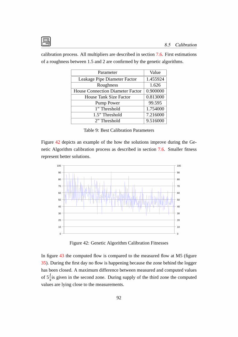
8.5 Calibration
calibration process. All multipliers are described in section7.6. First estimations
of a roughness between 1.5 and 2 are confirmed by the genetic algorithms.
Parameter Value
Leakage Pipe Diameter Factor 1.455924Roughness 1.626
House Connection Diameter Factor0.900000House Tank Size Factor 0.813000
Pump Power 99.5951” Threshold 1.754000
1.5” Threshold 7.2160002” Threshold 9.516000
Table 9: Best Calibration Parameters
Figure42 depicts an example of the how the solutions improve during the Ge-
netic Algorithm calibration process as described in section7.6. Smaller fitness
represent better solutions.
0
10
20
30
40
50
60
70
80
90
100
0
10
20
30
40
50
60
70
80
90
100
Figure 42: Genetic Algorithm Calibration Fitnesses
In figure 43 the computed flow is compared to the measured flow at M5 (figure
35). During the first day no flow is happening because the zone behind the logger
has been closed. A maximum difference between measured and computed values
of 5 lsis given in the second zone. During supply of the third zone the computed
values are lying close to the measurements.
92
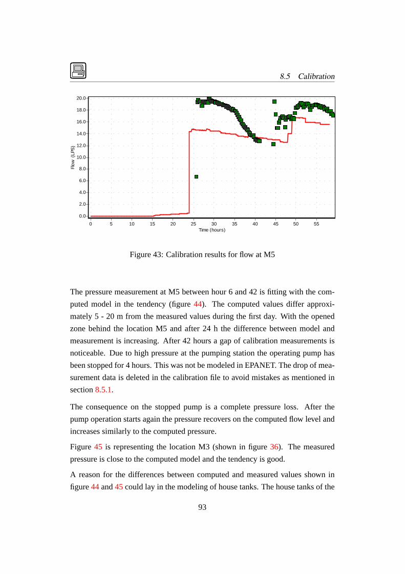
8.5 Calibration
Time (hours)5550454035302520151050
Flo
w (
LPS
)
20.0
18.0
16.0
14.0
12.0
10.0
8.0
6.0
4.0
2.0
0.0
Figure 43: Calibration results for flow at M5
The pressure measurement at M5 between hour 6 and 42 is fitting with the com-
puted model in the tendency (figure44). The computed values differ approxi-
mately 5 - 20 m from the measured values during the first day. With the opened
zone behind the location M5 and after 24 h the difference between model and
measurement is increasing. After 42 hours a gap of calibration measurements is
noticeable. Due to high pressure at the pumping station the operating pump has
been stopped for 4 hours. This was not be modeled in EPANET. The drop of mea-
surement data is deleted in the calibration file to avoid mistakes as mentioned in
section8.5.1.
The consequence on the stopped pump is a complete pressure loss. After the
pump operation starts again the pressure recovers on the computed flow level and
increases similarly to the computed pressure.
Figure45 is representing the location M3 (shown in figure36). The measured
pressure is close to the computed model and the tendency is good.
A reason for the differences between computed and measured values shown in
figure44and45could lay in the modeling of house tanks. The house tanks of the
93

8.5 Calibration
Time (hours)5550454035302520151050
Pres
sure
(m
)
120.0
110.0
100.0
90.0
80.0
70.0
60.0
50.0
40.0
30.0
20.0
10.0
0.0
-10.0
-20.0
-30.0
Figure 44: Calibration results for pressure at M5
Time (hours)5550454035302520151050
Pres
sure
(m
)
120.0
110.0
100.0
90.0
80.0
70.0
60.0
50.0
40.0
30.0
20.0
10.0
0.0
-10.0
Figure 45: Calibration results for pressure at M3
model are not equivalent to the house tanks hanging on a particular pipe in reality
to 100%.
94

8.5 Calibration
Some tank sizes of the model are too big, others are too small. This situation has
an effect on the pressure of course. An even higher influence on the inaccuracy
might stem from the distribution of leakage tanks in the network. Besides the
elevations have an accuracy of app. 25 metres only. The DEM is cross-checked
but differences have been ascertained. The measurement locations might lay up
to 25 metres higher than fixed in the model.
Time (hours)5550454035302520151050
Pres
sure
(m
)
65.0
60.0
55.0
50.0
45.0
40.0
35.0
30.0
25.0
20.0
15.0
10.0
5.0
0.0
Figure 46: Calibration results for pressure at M4
Measurement locations in the village can not be reflected with the computed
model easily. M4 and M7 are lying in densely populated areas. Despite the com-
puted pressure is close to the measured values.
The constant positive pressure over the first 24 h shown in figure47 is a problem
of EPANET which is not designed to model intermittent supply. It happens in
periods of empty pipes that EPANET shows pressures, even if the pipes are set on
“closed” (section8.3.6) because the zone is not supplied yet.
Nevertheless, the tendency of the model is fitting with the measurements. This
is also shown in figure47 representing location M7. Pressure level as well as
tendencies are fitting between computed and measured values.
Figure 48 represents a pressure measurement at location M2. This location is
the first on the way to Judayta and at the lowest point of all measurements. The
95
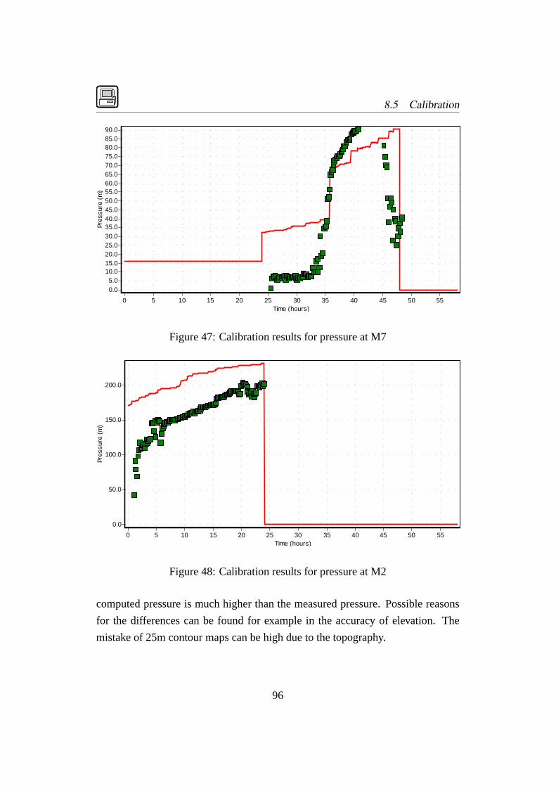
8.5 Calibration
Time (hours)5550454035302520151050
Pres
sure
(m
)
90.085.080.075.070.065.060.055.050.045.040.035.030.025.020.015.010.05.00.0
Figure 47: Calibration results for pressure at M7
Time (hours)5550454035302520151050
Pres
sure
(m
)
200.0
150.0
100.0
50.0
0.0
Figure 48: Calibration results for pressure at M2
computed pressure is much higher than the measured pressure. Possible reasons
for the differences can be found for example in the accuracy of elevation. The
mistake of 25m contour maps can be high due to the topography.
96

8.6 Comparison with a traditional Hydraulic Model
8.6 Comparison with a traditional Hydraulic Model
The necessity for creating hydraulic models of intermittent supply becomes clear
by the comparison with traditional network analysis models. The tolerated inaccu-
racy of traditional models in areas of intermittent supply shall be demonstrated. In
the following two traditional approaches to model the Judayta network are shown.
The first approach tries to simulate intermittent supply as far as possible with
nodal demands. It models the different zones in separated hydraulic models (sec-
tion 8.6.2). The demand of nodes depends on the operation of zones.
The second approach resembles the design of a continuous supply network. It
is described in section8.6.3. It consists of a one-zone model with a demand
calculated directly out of the billed consumption. The operation of zones and the
resulting change of demand are ignored.
8.6.1 Traditional Model Creation
The following parameters have to be adjusted in order to realize a traditional
model with nodal demand:
• Junction demands.
• Supply duration.
• Roughness.
• Pressure zones.
Junction Demands The process is similar to the process described for the gen-
eration of the generalized household storage tanks.
Supply duration Judayta can be divided into three zones while elements of the
network have to be shared by zones (e.g. pumping station). In this context the
important elements are the nodes (junctions). The junction theme gets a new
attribute “Duration” in the Database.
97
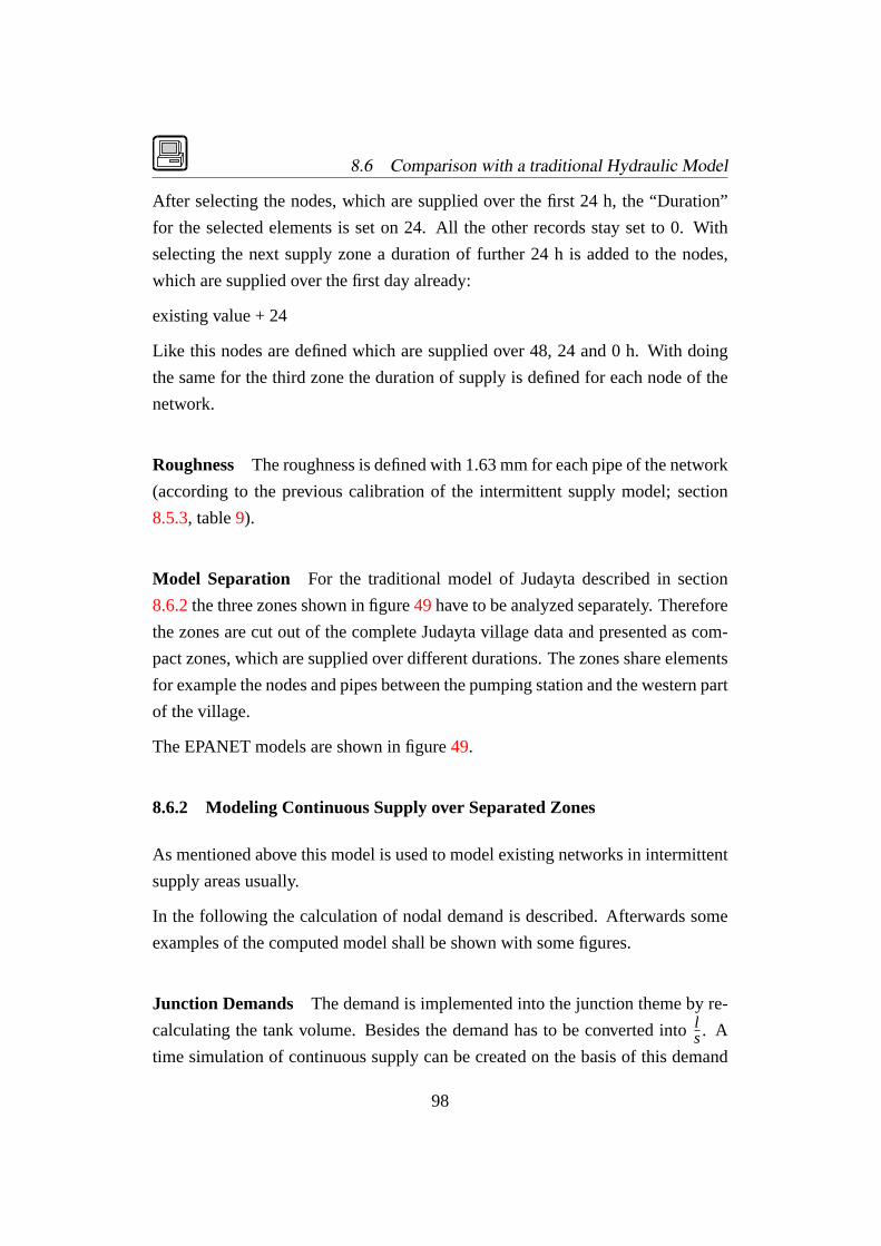
8.6 Comparison with a traditional Hydraulic Model
After selecting the nodes, which are supplied over the first 24 h, the “Duration”
for the selected elements is set on 24. All the other records stay set to 0. With
selecting the next supply zone a duration of further 24 h is added to the nodes,
which are supplied over the first day already:
existing value + 24
Like this nodes are defined which are supplied over 48, 24 and 0 h. With doing
the same for the third zone the duration of supply is defined for each node of the
network.
Roughness The roughness is defined with 1.63 mm for each pipe of the network
(according to the previous calibration of the intermittent supply model; section
8.5.3, table9).
Model Separation For the traditional model of Judayta described in section
8.6.2the three zones shown in figure49have to be analyzed separately. Therefore
the zones are cut out of the complete Judayta village data and presented as com-
pact zones, which are supplied over different durations. The zones share elements
for example the nodes and pipes between the pumping station and the western part
of the village.
The EPANET models are shown in figure49.
8.6.2 Modeling Continuous Supply over Separated Zones
As mentioned above this model is used to model existing networks in intermittent
supply areas usually.
In the following the calculation of nodal demand is described. Afterwards some
examples of the computed model shall be shown with some figures.
Junction Demands The demand is implemented into the junction theme by re-
calculating the tank volume. Besides the demand has to be converted intols. A
time simulation of continuous supply can be created on the basis of this demand
98

8.6 Comparison with a traditional Hydraulic Model
� �
�
� ��������� �
��
� �� � � ���
����� � � �� � ���
��
��
� ����� �
�
� ����
�
��
�
�
��
�
�
�
��
��
�
�
�
�
���
�������
�
�
�
��
�
� ��
(a) Fist Zone
�
�
� ����������
� � � � ������� � �� �
���
� �
�
��
�
���
�
�
����
�
�
��� �
� ����
���
� ���
�
���� �� ���
��
��
������
���
�
��
�
�
��� ����
��
�
�
�
��
��
� ��
(b) Second Zone
�
�
� ����������
� � � � ������� � �� �
���
� �
�
��
�
���
�
�
����
�
�
��
�
�� �
�
�
�
� �
���
� ����� �� ���
��
��
�
�
�
�
�
�
��
������
��� ����
�
�
�
����
�
�
�
��
(c) Third Zone
Figure 49: Traditional Model Zones
over 58hw. This duration is chosen for getting the opportunity of comparing results
of the traditional model with the approach of modeling intermittent supply.
mQs = Q3m/14hs/ht,s
· 158h
w·3600sh·1000·mS·mL
with
mQs= Average demand inls
Q3m= Consumption according to COBOSS during 3 month of the year inm3
3monthwith
14 w3month
hs= Time of supply according to operation of zones in h (24 h, 10 h)
99

8.6 Comparison with a traditional Hydraulic Model
ht,s= Total time of supply interval (58 h)
mL= Multiplier for considering Losses, estimated with 40%
mS= Peak factor
The peak factor is estimated as 1.4 [5]. The multiplier for considering losses is
justified by measurements of back flow at the pumping station. UFW are estimated
with 40% (section5.1).
Results A calibration of the model is difficult because of its condition. The
demand is not changing over the day because of house tanks in the distribution
network. Therefore the system is static.
Figure50 represents one of the best results of this model with a pressure of 7.4
bar. The computed pressure is close to an average value of the measurements.
During the first supply interval the computed values of the other locations are of
similar quality.
Time (hours)5550454035302520151050
Pres
sure
(m
)
120.0
110.0
100.0
90.0
80.0
70.0
60.0
50.0
40.0
30.0
20.0
10.0
0.0
Figure 50: Pressure at M5
Especially during the supply of the third zone an extreme sub-pressure can be no-
ticed at several locations (an example is given with figure51). Warnings because
of negative pressures are given by EPANET especially for this zone. In cases like
this the pump size or parameters for increasing the power are changed usually.
For reaching better results the pump speed has to be increased with 50%.
This essentially means that the respective models are broken.
100

8.6 Comparison with a traditional Hydraulic Model
Time (hours)5550454035302520151050
Pres
sure
(m
)
50.0
0.0
-50.0
-100.0
-150.0
-200.0
Figure 51: Pressure at M8
8.6.3 Continuous Supply as Designed
This model consists of one zone as mentioned above. The demand is calculated
directly out of the billed consumption without differentiation of nodes, which are
supplied 24 h, 48 h or 58 h in reality. Each node is getting the demand in depen-
dence on the specific consumption.
� �
�
� ��������� �
��
� �� � � �������� � � �� � ���
�� �
�
��
�
���
�
�
����
�
�
��
�
�� �
�
�
�
� ����
���
� ���
�
���� �
�
� ���
�
�
���
�
��
�
�
�
�
�
��
�
��
��
�
�
�
��
���
��
������
�
�
�
�
���
�
��
��
��� ����
��
�
�
�
�
����
��
�
�
��
Figure 52: Traditional Model of Node Demand
Junction Demand This approach is a simplification of the model described in
section8.6.2.
mQs = Q3m14 · 1
58hw·3600s
h·1000·mL ·mS
mQs= Average demand inls
Q3m= Billed consumption during 3 month of the year inm3
3monthwith 14 w3month
101
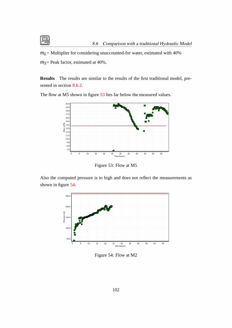
8.6 Comparison with a traditional Hydraulic Model
mL= Multiplier for considering unaccounted-for water, estimated with 40%
mS= Peak factor, estimated at 40%.
Results The results are similar to the results of the first traditional model, pre-
sented in section8.6.2.
The flow at M5 shown in figure53 lies far below the measured values.
Time (hours)5550454035302520151050
Flow
(LP
S)
20.0
19.0
18.0
17.0
16.0
15.0
14.0
13.0
12.0
11.0
10.0
9.0
8.0
7.0
Figure 53: Flow at M5
Also the computed pressure is to high and does not reflect the measurements as
shown in figure54.
Time (hours)5550454035302520151050
Pres
sure
(m
)
250.0
200.0
150.0
100.0
50.0
Figure 54: Flow at M2
102

8.6 Comparison with a traditional Hydraulic Model
8.6.4 Model Comparison
Both traditional models have been analyzed. These models do not reflect inter-
mittent supply. The point is that in reality tanks are filled in dependence on the
present pressure. The traditional model ignores this by modeling the consumption
as a nodal demand, which is pressure independent. As shown in figure51 this
continuous demand cannot be satisfied sometimes.
With the presented model of intermittent supply each node is getting that quantity
of water, which is offered at a specific time and location. The quantity of water,
which is running into a tank, depends on the pressure at this location and the
pressure is influenced mainly by filling tanks and quantity of leakage below.
In addition to this mistake of traditional models in intermittent supply areas, the
development of pressure, demand and flow over the time cannot be represented.
However the present approach can deliver these informations as shown in section
8.5.3. Advantages of the intermittent supply model are listed in the following:
• It is possible to show the filling level of house tanks over the time.
• The characteristic of intermittent supply to get water, if water is available,
in reliance to the pressure is implemented.
• The complete village can be modeled in one system based on valve control
rules for operating the zones automatically.
• The total mistake between computed model and measured values can be
cross-checked by pressure and flow diagrams, which can be created for each
location of the network (e.g. figure47). A calibration of traditional models
can be done over the total mistake only, because of linearity (see figure50).
• UFW is implemented as leakage with spatial reference. The traditional
models are implementing losses into demands.
103

9 Optimization of the Judayta Water Supply Net-
work
by STEFFENMACKE
A lot of problems with the water supply network in Judayta village are obvious
even without an hydraulic analysis. The extremely high pressure in the lower
supply areas is likely to cause a lot of damage to the expensive water meters as
well as leakage.
9.1 Background
To compare the current leakage rates in the Judayta network, the specific char-
acteristic loss can be used. The specific characteristic loss relates the leakage to
the supply time and length of the water network. Table10displays diameters and
lengths of pipelines in the Judayta water network.
DN Length in m
25 15950 12959100 1875150 4339200 16
Table 10: Pipelines Judayta
As the calculation of the specific characteristic loss does not take house connec-
tions into account the total length of water network amounts to 6.23 km. One sup-
ply period in Judayta lasts 58 hours in which 1658 cubic metres are unaccounted-
for. Hence the specific characteristic loss is:
qv =1658
58·6.23= 4.58
m3
m·kmIn the literature, the following specific characteristic loss is given as a high value
for underground containing seams[8]:
104

9.1 Background
qv = 0.6m3
km·h
qv = 0.6m3
km·hHowever, with the yet unknown amount of illegal consumption it can only be
estimated how much leakage participates in the unaccounted-for figure. The pri-
vatization of meter readings in the Al Koura district is likely to reduce illegal
consumption and ensure more reliable figures.
It is very important to realize that most of the actions described hereafter only have
a chance to succeed if the administrative actions succeed also. The administrative
measures are a precondition for the technical ones.
Figure 55: Leakage
As there are many leaks visible in Judayta (figure55 shows an example), a tech-
nical loss reduction program is likely to succeed. But the decision on technical
actions like a leak detection campaign should be delayed until more reliable meter
105

9.2 Pumping Station
readings are available for both the customer side and Judayta pumping station.
9.2 Pumping Station
Technicians reported that the Judayta pumping station is “one of the best” through-
out Irbid Governorate - in terms of leakage and operation. However the following
practical improvements can be made with only little effort.
9.2.1 Bulk Water Meters
One of the most important actions to be taken is the installation of the necessary
bulk water meters in Judayta pumping station. The current setup does not allow to
record the consumption of the villages properly: The unmetered back flow into the
well as well as additional overflow - which is also unmetered, make it impossible
to calculate a reliable water balance (appendixH).
In addition, the current records rely on the operator at the pumping station: He
has to record the supplied village together with the well production readings - a
process that is very likely to produce unnecessary errors.
The introduction of separate meters for the two pumping directions should also
be used to move the valves that operate the pipelines into the pumping station:
Currently they are located right in front of it. It should be evaluated whether it is
more practical to move the fence or to move the valves.
Only those new bulk meters will allow an accurate assessment of tank overflow
and back flow to the well.
Alternatives Water meters capable of operation under a pressure of 40 bar are
expensive, the water meters should therefore be installed between storage tank
and pumps. However this will still allow the operator to pump with the same set
of pumps into different directions.
Alternatively, the meters could be installed on a higher location in the network
- such a setup is not recommended as it would not allow to meter water losses
106

9.3 Rehabilitation of the Existing Reservoir
on the way from the pumping station to the meter location. Also a water meter
located within the pumping station grounds is more secure than other locations.
An incident during the logging campaign illustrates this: A logger was set on fire.
9.2.2 Storage Capacity
Currently the back flow from the tank to the well decreases the well pumping
efficiency by up to 11% (section5.1). The main problem is that the overflow takes
place in a way that is hardly noticeable by the operator: The noise of the pumps
does not allow to hear the water overflowing.
An automated pump control is not likely to succeed, as it would require proper
maintenance, which can not be guaranteed under the current circumstances.
The following actions could be used overcome the problem:
• Installation of an additional steel tank to increase the storage capacity. Over-
flow situations will be less likely with it.
• Installation of an overflow activated horn on the well.
• Motivation of the operator to takes measures against the overflow.
The operator motivation is the crucial part: Currently it is not possible to use
bonus salaries to motivate the personnel.
As the horn is much cheaper than the tank it should be installed first to avoid
a costly bad investment with the tank: With horn the operator has a chance to
minimize the overflow. The additional water meters will allow the supervision of
the operator.
9.3 Rehabilitation of the Existing Reservoir
The existing (but currently unused) reservoir with a capacity of 200 cubic metres
that was discovered during the altimeter survey makes it possible to change the
107

9.3 Rehabilitation of the Existing Reservoir
Figure 56: Existing Reservoir
mode of operation from intermittent to a continuous supply of water. Figure56
shows a photo of the reservoir.
Again, such an action is only likely to succeed if administrative actions take place
before: The intermittent supply is currently used as a rationing system that pre-
vents excessive illegal consumption by only providing water one or two days a
week. Continuous supply would allow the illegal consumers to waste more water.
Under the assumption that the privatization of the meter readings succeeds and
reduces the illegal consumption, the intermittent supply rationing could be aban-
doned.
The capacity of the reservoir is big enough to provide the average demand for
9 hours. This should be sufficient as the household storage tanks will not be
abandoned immediately and hence the demand curve will be relatively flat.
108

9.4 Establishment of a Booster Station
9.4 Establishment of a Booster Station
The existing Reservoir is not able supply the whole village because it does not
supply sufficient pressure. By establishing a booster station next to the reservoir
this problem could be solved.
In case the empty parcel next to the reservoir is not available for the booster sta-
tion, the installation of pumps on top of the reservoir can be evaluated as well as
submersible pumps in the reservoir.
The booster station will also allow to serve additional customers in the north-
eastern part of the village which can not be supplied currently - the pipelines are
already in place in this area.
According to table8, the average consumption of Judayta village was 2865 cubic
metres per week in the 2000 reading cycle. Assuming 30% UFW for the future
(section9.7), this yields a total demand of 6.16 litres per second for continuous
supply. A simple network model based on reservoir supply and the demand has
been created.
Figure 57: Reservoir Supply Pressures
Figure 57 shows a map containing the network pressures distribution obtained
from the network simulation model. The areas of pressures below 15 m in the
west of the village need to be supplied by the booster.
109

9.5 Pressure Reduction
9.5 Pressure Reduction
The re-use of the existing reservoir will reduce the pressure in the network. For
example, the peak pressure at the eastern village boundary - the most problematic
area - will drop from above 30 bar to approximately 20 bar. As the pressure influ-
ences leakage over-proportional (equation2, section7.3) the pressure reduction
will reduce the amount leakage accordingly.
The decision whether to use a pressure reduction valve (PRV) or not is a difficult
one. One the one hand, the huge elevation differences in the Judayta network
require different pressure zones, on the other hand, such valves are expensive and
need appropriate maintenance in order to function properly.
Orifice plates should be evaluated as alternatives to pressure reduction valves -
their advantage is that they are inexpensive. However they are not able to reduce
static network pressures and may therefore not be well suited for Judayta’s lower
supply zones.
Though pressure reduction valves or orifice plates may help to reduce the crit-
ical network pressures further, the decision whether to use them or not should
only be taken after intensive evaluation together with the personnel in charge -
it is inevitable that they support the ideas and have the knowledge maintain the
installations.
9.6 Cost Rating
The cost rating is based on a cost estimate in [5]. The unit rates are based on
recently completed contracts in Irbid governorate.
Only one pump is considered, as it is still possible to pump directly into the net-
work in case of a booster pump failure.
9.7 Cost Benefit Analysis
Some of the benefits from the described actions can not be expressed in mone-
tary terms - for example the continuous supply of water, the possibility to serve
110

9.7 Cost Benefit Analysis
Measure Quantity Unit rate in JOD Amount in JOD
Reservoir rehabilitation LS - 3000Additional steel tank 1 3000 3000Water meter at pumping station 1 1500 1500Water meter at reservoir 1 1500 1500Overflow horn LS - 500Network reconnections LS - 5000Pipeline DN 100 1500 m 15 22500Pumps Q=10m3/h, H=90m 1 4000 4000Total 41500
Table 11: Cost Rating
additional customers or the ability to obtain reliable flow measurements.
Similar pressure reduction measures in another village of the Al Koura district -
namely the Al Taibeh System - are expected to yield a reduction of the unaccounted-
for water figures from 50% to 30%[5]. Assuming the same increase in efficiency
for Judayta, it would be possible to increase the revenue from water by 20%.
The average revenue for water in rural areas is 0.140 JOD per cubic metre[5]. The
estimated surplus revenue is:
0.140JODm3 ·0.20·149000
m3
a= 4170
JODa
This indicates a pay back period of 10 years. For the example in [5] the pay back
period was less than two years - due to a reduction in pumping costs. For the
proposed actions the pumping costs will also decrease slightly due to the reduced
back flow to the well - this is not yet considered.
As Judayta pumping station also supplies other villages, it is likely that the cost
benefit analysis will improve if similar actions are taken for the remaining villages.
111

10 Acknowledgments
The authors would like to thank the following people who have helped them dur-
ing the semester in Jordan We would not have been able to do this without them.
They appear in alphabetical order.
• Torsten Czysz
• The Kachel Family
• Stephan Kugler
• Tuuli Mogk
• Mohammad Jalal
• Ghazi Qussous
• Lewis Rossman
• Jamil Shahade
• Kala Vairavamoorthy
112

REFERENCES
References
[1] DIN ISO 4064, Durchflussmessung von Wasser in geschlossenen Leitun-
gen, Zähler für kaltes Trinkwasser, Spezifikationen, Teil 1. Technical report,
Deutsches Institut für Normung e.V., 1981.
[2] Technische Mitteilungen Merkblatt W391, Wasserverluste in
Wasserverteilungsanlagen, Feststellung und Beurteilung. Technical
report, DVGW, Frankfut am Main, 1986.
[3] Jordan in Figures 1999. Department of Statistics, Amman, 2000.
[4] Multistage Centrifugal Pumps. JET, S.p.A - Via d. Grazoli, 53/a - Gavassa,
42100 Reggio Emilia (Italy), 2000.
[5] Abu Najim/Abu Zaitun/Kugler/Sukkar. Working Paper No. 127 - Financial
improvement through optimized Water Supply System operations on the ex-
ample of Al-Taibeh Distribution System. Technical report, OMS, Amman,
May 2000.
[6] Alder. Energieaufkommen und -verwendung in der österreichischen Volk-
swirtschaft im Jahr 1990, endgültige Energiebilanz 1990.Statistische
Nachrichten, (10):885–895, 1993.
[7] Booch/Jacobson/Rumbaugh.The unified software development process.
Addison-Wesley, Reading, 1999.
[8] Damrath/Cord-Landwehr.Wasserversorgung. B.G. Teubner, Stuttgart, 11th
edition, 1998.
[9] Dibona/Stone/Ockmann, editor.Open Sources: Voices from the Open
Source Revolution. O’Reilly, Cambridge, 1st edition, 1999.
[10] Fischer, editor.Der Fischer Weltalmanach 2001. Fischer Taschenbuch Ver-
lag, Frankfurt am Main, 2000.
113

REFERENCES
[11] Kunze/Kugler. Incorporating Water Loss Reduction Programme Jerash and
Irbid. Technical report, KfW, October 2000.
[12] Laenge/Kugler/Naouri. Working Paper No. 87 Pump Efficiency and Pump
Maintenance. Technical report, OMS Project, Amman, May 1998.
[13] Martinez/Conejos/Vercher. Developing an integrated model for water distri-
bution systems considering both distributed leakage and pressure-dependent
demands. Technical report, Universidad Polit´ecnica de Valencia, 1999.
[14] Mutschmann/Stimmelmayr.Taschenbuch der Wasserversorgung. vieweg,
Wiesbaden, 12th edition, 1999.
[15] Niemeyer/Gilles/Riggers.Reduction of Water Losses in Drinking Water Sup-
ply Systems in Developing Countries, volume 120 ofResearch Reports of the
Federal Ministry for Economic Cooperation and Development, Germany.
Weltforum Verlag, Cologne, 1996.
[16] Rossmann.EPANET 2 Users Manual. United States Environmental Protec-
tion Agency, Cincinnati, Ohio, September 2000.
[17] Savic/Walters. Genetic Algorithms for Least-cost Design of Water Distribu-
tion Networks. ASCE Journal of Water Resources Planning and Manage-
ment, 123(2):67–77, 1997.
[18] Snyder.Map Projections. ESRI, Redlands, 1994.
[19] Vairavamoorthy/Ali/Akinpelu/Lin. An Appropriate Design Tool For Inter-
mittent Water Supply Systems. Technical report, South Bank University,
London, 2000.
114

LIST OF FIGURES
List of Figures
1 Middle East . . . . . . . . . . . . . . . . . . . . . . . . . . . . .15
2 Jordanian Governorates . . . . . . . . . . . . . . . . . . . . . . .16
3 Irbid Governorate . . . . . . . . . . . . . . . . . . . . . . . . . .17
4 Al Koura Villages . . . . . . . . . . . . . . . . . . . . . . . . . .19
5 Water Loss . . . . . . . . . . . . . . . . . . . . . . . . . . . . .21
6 Unaccounted-For Water . . . . . . . . . . . . . . . . . . . . . . .22
7 Judayta pumping station . . . . . . . . . . . . . . . . . . . . . .27
8 Storage Tank at Judayta pumping station . . . . . . . . . . . . . .32
9 Operation of Judayta pumping station . . . . . . . . . . . . . . .33
10 Tank overflow measured by Bucket Fill. . . . . . . . . . . . . . .33
11 Bucket Fill Photo . . . . . . . . . . . . . . . . . . . . . . . . . .34
12 Water Meter at Well No. 1 . . . . . . . . . . . . . . . . . . . . .35
13 Location of Domestic Meter Tests . . . . . . . . . . . . . . . . .36
14 Flow during Supply Period . . . . . . . . . . . . . . . . . . . . .37
15 Flow after Supply Period . . . . . . . . . . . . . . . . . . . . . .37
16 Air Release Valve Installation . . . . . . . . . . . . . . . . . . .38
17 Result of Meter Test at Location A . . . . . . . . . . . . . . . . .39
18 Result of Meter Test at Location B . . . . . . . . . . . . . . . . .39
19 UML class inheritance . . . . . . . . . . . . . . . . . . . . . . .47
20 Extract: UML Static State Analysis Diagram . . . . . . . . . . .48
21 Altimeter Spot Heights in Judayta . . . . . . . . . . . . . . . . .54
115

LIST OF FIGURES
22 Virtual Line Validity . . . . . . . . . . . . . . . . . . . . . . . . 62
23 Virtual Line Creation . . . . . . . . . . . . . . . . . . . . . . . .62
24 Bit-coding Supply Zones . . . . . . . . . . . . . . . . . . . . . .64
25 Calibration Influences . . . . . . . . . . . . . . . . . . . . . . . .64
26 Allele Mutation . . . . . . . . . . . . . . . . . . . . . . . . . . .66
27 Reproduction with Crossover . . . . . . . . . . . . . . . . . . . .67
28 Calibration Process . . . . . . . . . . . . . . . . . . . . . . . . .69
29 Zoning during Summer Time . . . . . . . . . . . . . . . . . . .71
30 Zoning during Winter Time . . . . . . . . . . . . . . . . . . . . .71
31 Join of Tabular and Spatial Data . . . . . . . . . . . . . . . . . .74
32 Centre Point Creation . . . . . . . . . . . . . . . . . . . . . . . .75
33 Creation of Tanks with characteristic Elevation . . . . . . . . . .76
34 Check Valves . . . . . . . . . . . . . . . . . . . . . . . . . . . .82
35 Flow Logger Locations . . . . . . . . . . . . . . . . . . . . . . .85
36 Pressure Logger Locations . . . . . . . . . . . . . . . . . . . . .86
37 Pump Curve . . . . . . . . . . . . . . . . . . . . . . . . . . . . .86
38 Pressure on the first Day . . . . . . . . . . . . . . . . . . . . . .87
39 Pressure on the second Day . . . . . . . . . . . . . . . . . . . . .87
40 Pressure an Flow at Logger M5 . . . . . . . . . . . . . . . . . . .88
41 Pressure during the last 10 hours . . . . . . . . . . . . . . . . . .88
42 Genetic Algorithm Calibration Fitnesses . . . . . . . . . . . . . .92
43 Calibration results for flow at M5 . . . . . . . . . . . . . . . . . .93
44 Calibration results for pressure at M5 . . . . . . . . . . . . . . .94
45 Calibration results for pressure at M3 . . . . . . . . . . . . . . .94
46 Calibration results for pressure at M4 . . . . . . . . . . . . . . .95
116

LIST OF FIGURES
47 Calibration results for pressure at M7 . . . . . . . . . . . . . . .96
48 Calibration results for pressure at M2 . . . . . . . . . . . . . . .96
49 Traditional Model Zones . . . . . . . . . . . . . . . . . . . . . .99
50 Pressure at M5 . . . . . . . . . . . . . . . . . . . . . . . . . . .100
51 Pressure at M8 . . . . . . . . . . . . . . . . . . . . . . . . . . .101
52 Traditional Model of Node Demand . . . . . . . . . . . . . . . .101
53 Flow at M5 . . . . . . . . . . . . . . . . . . . . . . . . . . . . .102
54 Flow at M2 . . . . . . . . . . . . . . . . . . . . . . . . . . . . .102
55 Leakage . . . . . . . . . . . . . . . . . . . . . . . . . . . . . . .105
56 Existing Reservoir . . . . . . . . . . . . . . . . . . . . . . . . .108
57 Reservoir Supply Pressures . . . . . . . . . . . . . . . . . . . . .109
117

LIST OF TABLES
List of Tables
1 Population Figures . . . . . . . . . . . . . . . . . . . . . . . . .18
2 Family Statistics . . . . . . . . . . . . . . . . . . . . . . . . . .18
3 Subscriber Statistics . . . . . . . . . . . . . . . . . . . . . . . . .18
4 Palestine Grid Coordinate System Parameters . . . . . . . . . . .24
5 Pipe Materials in the Al Koura Distribution Network . . . . . . .28
6 Network Data Update Statistics . . . . . . . . . . . . . . . . . . .52
7 Cross-Check of DEM with Spot-Heights . . . . . . . . . . . . . .55
8 COBOSS Data Summary . . . . . . . . . . . . . . . . . . . . . .72
9 Best Calibration Parameters . . . . . . . . . . . . . . . . . . . .92
10 Pipelines Judayta . . . . . . . . . . . . . . . . . . . . . . . . . .104
11 Cost Rating . . . . . . . . . . . . . . . . . . . . . . . . . . . . .111
118

LIST OF TABLES
119

IndexAbbreviations,12
AGWA, 12
Al Koura, 18
Algorithms, Genetic,65
Altimeter,25
Altimeters,53
Amman,15
API, 12
ArcInfo, 24, 42
ArcView, 42, 56
ASCII, 12, 73, 89
aSL,12
AVENUE, 57
Bitcode,63, 122
Calibration,63
CASE,45
CDC,12, 26
class,46
COBOSS,12, 23
Coded Value Domains,50
Connectivity,51
CSS,12, 23
CV, 12
data types,43
DC Water Design Extension,76, 77
DEM, 12, 25
demand, pressure-dependent ,59
dia,46
diagram,46
discharge,60
DLS, 12
DN, 12
energy,15
EPANET,25, 56
ESRI,12, 26
Evolution,67
Extension,42, 57
free software,46, 57
generalization,47
Genetic Algorithms,65
geometric network,51
GI, 12, 26
GIS,12
GNOME,12
GNU, 12
GTZ, 12
GUI, 13
HA, 13
HDPE,13
Intermittent Supply,56
Irbid, 17
IRR, 13
IRWA, 13
JICA, 13
JOD,13, 16
Jordan,15
120

INDEX
Jordanian Dinar,16
JTM, 24
KfW, 13, 19
LEMA, 13
LGPL, 13, 57
LS, 13
MWI, 13
OMG, 13, 44
OMS,13
orifice,60
Palestine Grid,24
PE,13
PK, 13, 23, 73
PMU, 13
pressure-dependent demand,59
PRV,13, 110
PSP,13, 20
quality,25
Range Domains,50
RJGC,13, 24, 53
SCADA, 14
Software,41
SOGREAH,14
Sogreah,22
SOV,14
SQL,14
Supply, Intermittent,56
Survey,25
Tank,58
UFW, 14, 21
UML, 14, 44
Unaccounted-for water,21
USAID, 14
Virtual Line, 61
Virtual Lines,123
WAJ, 14, 25
water quality,25
WLRP,20
XML, 14, 46
121

A DC Water Design Extension Manual
by STEFFENMACKE
This Manual describes the DC Water Design Extension Version 2.00.
This Document uses Terminology from ArcView and EPANET. Please refer to the
respective documentation for in-depth explanations.
A.1 What is the DC Water Design Extension?
The DC Water Design Extension is an Extension to ESRI’s ArcView GIS soft-
ware. Version 2.00 integrates the EPANET 2.00 hydraulic modeling software with
ArcView. It allows to store, edit and retrieve EPANET hydraulic models including
all options in ArcView. Also it is possible to run the EPANET hydraulic analysis
from ArcView and load the results into the GIS. Loading of EPANET models to
ArcView is not yet implemented.
A.1.1 Concepts
Network Traces Network Traces are be useful to solve problems related to the
network geometry. It is possible for example to check the connectivity of the
network features in a model. Through specifying network features at which the
trace should stop, it is possible to isolate supply zones.
Bit codes Bit codes are stored as integer numbers in GIS data. They provide a
powerful method to store hydraulic models in GIS data. The underlying principle
is very simple:
• The models are numbered
• Each bit represents one supply zone
122

A.2 Installation
• If the bit is set (1) than the network feature is used in the respective model.
Otherwise (0), the feature is not used in the model.
• The different values are assembled by arithmetic addition.
The bit numbering starts with 0. A temporary field should be used in order to
correctly perform the addition of two bit codes. !
Virtual Lines Virtual Lines provide a concept to convert GIS point data (pumps
or valves) into the lines used by the hydraulic analysis software. The conversion is
done automatically when the GIS data is exported to the hydraulic model. Virtual
Lines require exactly two pipes connected to each pump or valve. In addition, the
two pipes must have the same digitizing direction (which will be the flow direction
in the hydraulic model).
A.2 Installation
A.2.1 How to obtain the DC Water Design Extension
For DORSCH Consult staff, the DC Water Design Extension is available from the
DC GIS Database (Lotus Notes).
All others can obtain the DC Water Design Extension including documentation
and source code from the DC Water Design Extension homepage:
http://dcwaterdesign.sourceforge.net
To ease the installation process, the installer executable (setup program) is usually
the best choice.
A.2.2 Requirements
• ArcView 3.0 or higher
• Windows 95, 98, ME, NT or 2000 in order to export EPANET files
123

A.3 Usage
• EPANET 2.0 or higher is needed in order to run a hydraulic analysis
• An (ANSI SQL compliant) ODBC connection is needed in order to import
hydraulic analysis results
A.2.3 Setup
In order to install the DC Water Design Extension, one has to run the installer exe-
cutable. After accepting the license (sectionA.5), the installer prompts the user to
select the installation path. The installation path should be the path to ArcView’s
EXT32 folder. Usually this should be the default path (c:\ESRI\av_gis30\arcview\EXT32).
It might differ for custom ArcView installations. Than it has to be chosen which
components of the extension should be installed. In general, one should install all
the components of the extension.
If it is intended to use e.g. a newer version of the XSLT parser and the new
version is already installed, the user might choose not to install the XSLT parser!
that comes with the extension. However, this option should be left to the advanced
user.
A.3 Usage
A.3.1 General Usage
Extension loading
1. Start ArcView
2. Open the Extensions Dialog (File->Extensions ...)
3. Select the DC Water Design Extension (Put a checkmark in the box on the
left side).
4. After the Extension is loaded, the Setup Dialog provides information about
several settings. The settings should not be changed without profound knowl-
edge of their functionality.
124

A.3 Usage
A.3.2 Quick Start Guide
1. Load the Extension
2. Open a View
3. Add Themes to the View. The themes should describe the water supply
network. Junctions, pipes and reservoirs would comprise a simple network.
The attributes of the themes must adhere to the ArcView/EPANET Data
Model (appendicesB,C). ArcView field aliases can be used to map the
fields correctly.
4. Click on the EPANET Themes button. Select the appropriate Themes.
5. Choose “Make EPANET Model” from the DC Water Design menu
6. If the last step does not yield any errors, an EPANET input file can be cre-
ated now. Choose “Write EPANET File” from the DC Water Design menu.
Choose filename and location.
7. Fire up EPANET and open the created file (*.inp).
A.3.3 Project GUI
The DC Water Design Extension extends the Project GUI by adding a new Menu,
called DC Water Design Extension. The Menu contains the following choices:
Setup Shows the Setup Dialog.
The Setup Dialog includes an option to choose the language of the Extension.
Currently supported are the following localizations:
• English
• German
Note that the Localization is not completed yet. It is therefore recommended that
the language is set to English. i
125

A.3 Usage
EPANET Tables Displays the EPANET Tables Dialog.
The Tables in the dialog are used to to store non-spatial EPANET data with Ar-
cView. Typical examples of such data are pump curves or hydraulic analysis op-
tions. Before it is possible to use a table with the DC Water Design Extension, it
has to be loaded into ArcView. Refer to the ArcView documentation for informa-
tion on how to load tables into ArcView.
Result Tables Opens the Result Tables Dialog.
The Result Tables are used to store the results of a hydraulic analysis. There are
two tables, one for node results and one for link results. For performance reasons
it is recommended to use a RDBMS such as mySQL for storing the data. As of
version 2.00, the DC Water Design Extension has only been tested with mySQL
result tables.
About DC Water Design Extension Displays information about the DC Water
Design Extension License. SectionA.5 contains details on the license.
A.3.4 View GUI
The DC Water Design Extension extends the ArcView View GUI with the follow-
ing elements:
• A new Menu called “DC Water Design”
• Buttons
• Tools
• Three pop-up menus
The pop-up menus are available through clicking the right mouse button over a
network feature.
The additional functionality is explained below.
126

A.3 Usage
Write EPANET file Exports the hydraulic model to an EPANET input file.
The model has to be complete, running “Make EPANET Model” and “Check
EPANET Model” is advisable especially for the novice user before exporting the
EPANET input file.
The resulting EPANET input file has the extension *.inp. The *.xml-file is just an
intermediate format (temporary file). i
Run EPANET Calculation Exports the hydraulic model to an EPANET input
file, runs the analysis and loads the results into ArcView.
The model has to be complete, running “Make EPANET Model” and “Check
EPANET Model” is advisable especially for the novice user before exporting the
EPANET input file.
After the analysis has been completed, the report created by EPANET is displayed
in a window and the user is prompted to select a time step for which the results
will be loaded.
Load Results for step ... Loads the results of an EPANET hydraulic analysis
to ArcView.
The hydraulic analysis has to be run from ArcView in order to to enable this
feature. The user is prompted to select the time step for which the results should
be loaded.
Make EPANET Model Creates the line-node structure required by EPANET.
This function fills the fields node1 and node2 in the links table with the dc_ids of
the connected nodes. The fields will be overwritten by this function, therefore the
user has to confirm the action before the script run.
After completion, a report gives an overview of the created model. Model creation
errors are also reported. In case of such errors, the features in question are selected
after the run.
If there are reports about inconsistent flow direction at pumps or valves, the “Flip
Polylines” tool of the extension can be used to correct the errors.
127

A.3 Usage
EPANET Themes Opens the EPANET themes dialog.
The themes dialog is used to select the themes used in the hydraulic model. The
line and node theme are required, other themes are optional and can be switched
off with the check boxes on the right side.
Most of the extension functions require that the EPANET themes are properly set
up in this dialog. Setting up the themes should be the first step when using the!
extension. The settings of the EPANET themes dialog are also used to determine
which themes should be edited.
EPANET Tables Displays the EPANET tables dialog.
The tables in the dialog are used to to store non-spatial EPANET data with Ar-
cView. Typical examples of such data are pump curves or hydraulic analysis op-
tions. Before it is possible to use a table with the DC Water Design Extension, it
has to be loaded into ArcView. The ArcView documentation contains information
on how to load tables.
Valve Control Allows to set valve states according to EPANET Controls.
If a controls table is registered with the Extension (see EPANET Tables Dialog),
the user is offered to select the controls he would like to apply. All chosen controls
are applied: The status of the respective valves is set to “open” or “closed” de-
pending on the controls. This is very useful in combination with Network Traces
as the extension allows to stop traces at closed valves.
Make House Connections Creates a straight pipe between tanks and junctions
which share an id.
This function requires some preparatory work: Each tank of the tanks theme needs
to know to which junction it should be connected. This is expressed with a field
in the tanks attribute table that contains the dc_id of the junction the tank should
connect to. Such fields can be established e.g. by using the spatial join function
of the ArcView Geoprocessing Wizard.
128
A.3 Usage
Note that this functionality has been included mainly for the purpose of modeling
intermittent supply with household storage tanks. It might be taken out or in futurei
versions of the DC Water Design Extension. In fact, the best solution will be to
create another extension specialized on intermittent supply modeling that depends
on the DC Water Design Extension.
Create Supply Strings Calculates a coded text that shows when a node is sup-
plied with water.
This might only be used after successfully running an EPANET hydraulic analysis
from ArcView. The function will query the the nodes results table for pressures
above zero. Each pressure above zero will yield a “1” in the supply string, a
pressure below or equal zero will yield a “0” in the supply string. For each node,
the supply strings are written to a user-selectable text field. The field has to been
long enough to contain as many characters as there are time steps in the EPANET
results.
Note that this functionality has been included mainly for the purpose of modeling
intermittent supply with household storage tanks. It might be taken out in futurei
versions of the DC Water Design Extension. The ideal solution will be to create
another extension specialized on intermittent supply modeling that depends on the
DC Water Design Extension.
Calculate Pipe Length For Junctions This function calculates the length of
the pipes connected to a junction.
A user selectable number field in the junctions attribute table is filled with the
length of the pipes connected to each junction. In order not to double the overall
pipe length, each pipe length is divided by two. Thus every part of a pipe is
assigned to the nearest node.
Clip Themes by Bitcode Creates new themes with features which have the
same bit set in a bit code.
129

A.3 Usage
The functions works with all active themes in the view. First, the user is prompted
to select the bit which has to be set for the clipped themes. Then the field contain-
ing the bit code has to be chosen. (The script assumes that the bit code field names
are the same throughout all the active themes.) The user can select the filename
and location for each clipped theme. He can also choose whether the new themes
should be added to the view.
Bit codes make it possible to use the same network features in different supply
zones. This requires extraction of the features into separate themes. See section
A.1.1 for details on bit codes.
About DC Water Design Extension Displays information about the DC Water
Design Extension License. See sectionA.5 for the license details.
Flip Polylines This tool allows to flip the digitizing direction of lines.
The theme containing the lines to be flipped has to be set up as the pipe theme in
the EPANET themes dialog. Simple clicking on the line will switch the digitizing
direction.
Tip: ArcView’s symbology can be used to display the digitizing direction with
arrowheads. ?
Move Nodes A tool to move network nodes including rubber-banding.
With this tool it is possible to move network nodes (junctions, tanks, reservoirs,
pumps, valves) along with the connected pipes. The network stays intact and fully
connected (rubber-banding).
The respective themes have to be registered with the extension in the EPANET
themes dialog.
Split Pipe (Add Junction) A tool that allows to split a pipe into two pipes.
Adds a new junction at the split point.
130
A.3 Usage
The two new pipes inherit the attributes from the original pipe. However, the
length gets recalculated based on the shapes.
Pipe and junction themes have to be chosen in the EPANET themes dialog.
Edit Pipe Vertices Allows to re-shape pipes.
Vertices determine the route of a pipe. The tool makes it possible to move all the
vertices of a pipe. Additional, it is possible to add vertices to the pipe. Unlike the
ArcView tool “Vertex Edit”, “Edit Pipe Vertices” ensures network connectivity -
it is impossible to disconnect a pipe from a node with this tool.
The pipe theme has to be set up in the EPANET themes dialog in order to use this
tool.
Note that the pipe length is not recalculated. The pipe length has to be calculated!
manually in the pipe theme attribute table. The Questions and Answers section of
this manual contains an entry that deals with calculating the pipe length.
Change Node Class A tool to convert nodes from one class to another.
The Change Node Class tool allows to convert e.g. a junction into pump. At-
tributes shared between the two classes are copied. After selecting an existing
node, the user is prompted to select the class to which the node should be moved.
The old node is deleted in order to prevent node duplication that would corrupt
the hydraulic model.
Obviously, the respective themes have to be registered with the extension in the
EPANET themes dialog.
Delete Feature A tool to delete network features.
Allows one-click deletion of network features. The user is prompted to confirm
the deletion. It is important to know that there’s no undo support with the DC
Water Design Extension.
The themes containing features that should be deleted have to be selected in the
EPANET Themes dialog.
131

A.3 Usage
Digitize Junction The Digitize Junction tool is used to digitize junctions.
The junctions are added to the junction theme selected in the EPANET themes
dialog.
Digitize Pipe The Digitize Pipe tool is used to digitize pipes.
The pipes are added to the pipe theme selected in the EPANET themes dialog. In
order to maintain the network integrity, the tool automatically adds junctions at
the pipe end if the pipe end does not snap onto an existing node.
Digitize Tank The Digitize Tank tool is used to digitize tanks.
The tanks are added to the tank theme selected in the EPANET themes dialog.
Digitize Valve The Digitize Valve tool is used to digitize valves.
The valves are added to the valve theme selected in the EPANET themes dialog.
The tool is disabled if the valve theme is not enabled in the EPANET themes
dialog.
Digitize Reservoir The Digitize Reservoir tool is used to digitize reservoirs.
The reservoirs are added to the reservoir theme selected in the EPANET themes
dialog. The tool is disabled if the reservoir theme is not enabled in the EPANET
themes dialog.
Digitize Pump The Digitize Pump tool is used to digitize pumps.
The pumps are added to the pump theme selected in the EPANET themes dialog.
The tool is disabled if the pump theme is not enabled in the EPANET themes
dialog.
132
A.3 Usage
Show Pipe Table Entry Pop-up menu item that allows to show the attributes of
a pipe.
Right-clicking on a pipe and selecting this menu item opens the pipe attribute
table, selects and promotes the pipe.
The appropriate pipe theme has to be selected in the EPANET themes dialog.
Edit Pipe Table Entry Pop-up menu item allowing to edit the attributes of a
pipe.
Right-clicking on a pipe and selecting this menu item opens the pipe attribute
table, makes it editable, selects and promotes the pipe record. After that, the
attributes of the pipe can be edited. The DC Water Design Extension currently
provides no undo functionality.
Select Connected Pipes Pop-up menu item that allows to trace the pipes con-
nected to the selected pipe.
Right-clicking on a pipe and selecting this menu item opens a dialog that offers
node types at which the trace should stop. Multiple types can be selected. During
the trace, the status bar informs what percentage of the network has been covered
by the trace so far. The progress bar will not make it to 100% unless the network
is fully connected and no stopping features have been selected. The connected
pipes up to all stop points are returned as the selection.
Show Node Table Entry Pop-up menu item that shows the attributes of a node.
Right-clicking on a node and selecting this menu item opens the node attribute
table, selects and promotes the pipe.
The appropriate node theme has to be selected in the EPANET themes dialog.
Edit Node Table Entry Pop-up menu item that allows to edit the attributes of a
node.
133

A.3 Usage
Right-clicking on a node and selecting this menu item opens the node attribute
table, makes it editable, selects and promotes the node record. After that the
attributes of the node can be edited. Important notice: Undo is not supported by
the extension.
Select Node Selects the current node.
Adds the current node to the selection in the node theme.
The appropriate node themes has to be selected in the EPANET themes dialog.
A.3.5 Table GUI
Bitcode Calculator The Bitcode Calculator is accessible from the button bar of
the table GUI. It is disabled unless the table is editable and a numerical field is
selected.
• Upon clicking on the Bitcode Calculator button, the user is prompted to
select the bits he wants to set.
• After choosing OK, the bit code will be calculated and written to all the
selected records.
• If no records are selected the bit code is written to all the records in the
table.
The field used to store the bit codes should have no decimal places.
Bitcodes are a concept that allows to transparently share network features in mul-
tiple supply zones. SectionA.1.1contains more information on bit codes.
A.3.6 API Documentation
This section documents extension scripts that could be used from the field calcula-
tor or in queries. In Addition, the script responsible for the localization (extension
dictionaries) is documented. In general, the API (Application Programming Inter-
face) documentation should only be of concern for programmers.
134

A.3 Usage
DCWatDes.Bitcode.or performs a bitwise or operation on integer numbers
integer DCWatDes.Bitcode.or(integer a, integer b)
a bit-coded integer
b bit-coded integer
Returns: the result of the bitwise a or b as an integer
The following AVENUE code can be used in the field calculator to perform of a
bitwise or-operation on the fields a and b:
av.run("DCWatDes.Bitcode.or", {[a], [b]})
DCWatDes.Bitcode.and performs a bitwise and operation on integer numbers
integer DCWatDes.Bitcode.and(integer a, integer b)
a bit-coded integer
b bit-coded integer
Returns: the result of the bitwise a and b as an integer
The following AVENUE code can be used in the field calculator to perform of a
bitwise and-operation on the fields a and b:
av.run("DCWatDes.Bitcode.and", {[a], [b]})
DCWatDes.Bitcode.isSetAsNumber return whether the n-th bit of an integer
is set or not
integer DCWatDes.Bitcode.isSetAsNumber(integer a, integer n)
a bit-coded integer
n number of the bit to check
135

A.4 Questions and Answers
Returns: an integer of value 1 in case the n-th bit is set, 0 otherwise
The following AVENUE query can be used to select all the records which have
set the 4th bit in the example field (usable with the query tools of view and table
GUI):
av.run("DCWatDes.Bitcode.isSetAsNumber",{[example], 3}) = 1
Note that the bit numbering starts at 0. “= 1” is used to convert the numbers 0 and
1 to the boolean values to true or false, respective.
DCWatDes.i18n.createDictionaries Creates the localization dictionaries of the
extension.
In order to add another dictionary, the new dictionary has to be created first:
dicNew= Dictionary.make(100)
Next, dictionary entries can be added to the new dictionary:
dicNew.add(“English Term”, “New translated term”)
The German dictionary contains most of the terms that have to be translated. After
all the terms have been added to the new dictionary, the Dictionary has to be added
to the Dictionary of Dictionaries:
_dcwDicDictionaries.add(“tr”, dicNew)
Where “tr” is the text that shows up in the setup dialog of the extension.
A.4 Questions and Answers
Why is there no graphical user interface to the DCWatDes.Bitcode.* func-
tions? The provided AVENUE functions are more flexible this way. Bit codes
can be useful for quite a number of operations. Try using the functions with the
field calculator and the query. Examples are given inA.3.6.
What is the Setup Dialog for? The Extension depends on several software
packages. The Setup Dialog allows to choose other versions of these software
packages than the ones supplied with the Extension itself.
136

A.4 Questions and Answers
Why is Version 2.00 not working with Pipe 2000 anymore? The Pipe 2000
data model, API and documentation are inferior to EPANET. Full integration of
Pipe 2000 into ArcView was impossible. With EPANET it is possible to store the
complete model, including all hydraulic analysis options in the GIS.
How do I recalculate the pipe length for all the pipes?
1. Open the attribute table of the pipe theme.
2. Make sure that the pipe theme is editable.
3. Make sure that no records are selected.
4. Click on the heading for the length field.
5. Click on the field calculator button.
6. Enter the following line into the value field:
[Shape].returnLength
7. Click OK.
I get strange errors when I try to create the EPANET model. What can I do?
Try the following:
• Try “Check EPANET model”. This helpful to resolve duplicate IDs.
• Have a close look at the erroneous features: Often accidentally duplicates
features cause trouble.
I made a mistake. Why is undo not working? Undo support had to be taken
out for the sake of editing multiple themes at the same time. Make frequent back-
ups. You have been warned. !
I found a bug in the Extension. What should I do? Please send your bug
reports to [email protected]
137

A.5 Copyright
A.5 Copyright
DC Water Design Extension 2.00. This ArcView Extension integrates EPANET
with ArcView.
Copyright (C) 1998-2001 DORSCH Consult
This library is free software; you can redistribute it and/or modify it under the
terms of the GNU Lesser General Public License as published by the Free Soft-
ware Foundation; either version 2.1 of the License, or (at your option) any later
version.
This library is distributed in the hope that it will be useful, but WITHOUT ANY
WARRANTY; without even the implied warranty of MERCHANTABILITY or
FITNESS FOR A PARTICULAR PURPOSE. See the GNU Lesser General Public
License for more details.
You should have received a copy of the GNU Lesser General Public License along
with this library; if not, write to the Free Software Foundation, Inc., 59 Temple
Place, Suite 330, Boston, MA 02111-1307 USA
AppendixD contains a copy of the GNU Lesser General Public License. ?
138
B ArcView/EPANET Data Model
This document describes version 2.00 of the ArcView/EPANET Data Model. Note
that the units will change if EPANET is not set to use litres per second (LPS) as
units. Refer to the EPANET documentation (especially the toolkit help) for further
information.
B.1 Identity
Inherited by Feature
Inherited by Pattern
Inherited by Curve
• dc_ID: string Unique ID throughout the whole database. Should not con-
tains spaces.
B.2 Node
Inherits from Feature
Inherited by Junction
Inherited by Tank
Inherited by Reservoir
Inherited by VirtualLine
• Shape:Point Spatial data.
• Elevation:float Elevation above Sea Level in m.
• result_demand:floatEPANET analysis result: Demand in litres per second.
• result_head:float EPANET analysis result: Total Head in m.
• result_pressure:float EPANET analysis result: Pressure in m.
139

B.3 Junction
• ElevationSource:CodedValueInteger field containing a coded value that
describes the origin of the elevation information for this node. The follow-
ing values have been used in the Al Koura project:
– 0: Unknown Source
– 1: 100 m Contours DEM
– 2: SOGREAH Procedure models
– 3: Altimeter Survey
– 4: Paper maps
– 5: estimated
– 6: 25 m Contours DEM
B.3 Junction
Inherits from Node
• Demand:float Base demand flow in litres per second.
• Pattern:string Demand Pattern ID. If no demand pattern is supplied then
the junction follows the Default Demand Pattern provided in the Options
Table, or Pattern 1 if no Default Pattern is specified. If none of the patterns
exist, the demand will remain constant.
B.4 Tank
Inherits from Node
• Initiallevel: float Initial water level above the tank bottom level (the eleva-
tion field) in m.
• Minimumlevel: float Minimum water level above the tank bottom level in
m.
140

B.5 Pump
• Maximumlevel:float Maximum water level above the tank bottom level in
m.
• Diameter:float Nominal Diameter of the tank in m. If a volume curve is
supplied this can be any non-zero number.
• Minimumvolume:float The minimum volume of the tank in cubic metres.
Can be zero.
• Volumecurve:stringThe id of the volumecurve - for non-cylindrical tanks.
B.5 Pump
Inherits from VirtualLine
• Properties:string EPANET properties of the pump. Keyword(s) followed
by value(s). Keywords consist of:
– POWER pump power in kW
– HEAD id of the head curve describing this pump
– SPEED relative speed of the pump: 1.0 is normal, 0 means that the
pump is off.
– PATTERN id of the time pattern describing pump operation.
• power_kw:integerThe power of the pump in kW.
B.6 Valve
Inherits from VirtualLine
• Diameter:integerDiameter of the valve in mm.
• Type: string Type of the valve. The following EPANET valve types are
valid:
141

B.6 Valve
– PRV pressure reducing valve
– PSV pressure sustaining valve
– PBV pressure breaker valve
– FCV flow control valve
– TCV throttle control valve
– GPV general purpose valve
Additional valve types supported by the DC Water Design Extension:
• CV check valve
– SOV shutoff valve
EPANET models these as pipes. The extension will create them on the fly.
• Setting: string Valve type dependent setting. The setting field takes the
following values for the different valve types:
– PRV the pressure in m
– PSV the pressure in m
– PBV the pressure in m
– FCV the flow in litres per second
– TCV the loss coefficient
– GPV the id of the head loss curve
– CV the setting value will be mapped to the status field of the pipe
– SOV the setting value will be mapped to the status field of the pipe
• Minorloss:float Minor loss coefficient of the valve.
142

B.7 Pipe
B.7 Pipe
Inherits from Feature
• Shape:PolylineSpatial data.
• node1:stringStart node dc_id.
• node2:stringEnd node dc_id.
• length:float The length of the pipe in m.
• diameter:integerNominal pipe diameter in mm.
• roughness:float Pipe roughness coefficient in mm.
• minorloss:float Minor loss coefficient.
• status:stringStatus of the pipe. The following values are valid:
– OPEN
– CLOSED
– CV (check valve)
• Material: CodedValueInteger field containing a coded value describing the
material of the pipe. The following values have been used in the Al Koura
project:
– 0: steel
– 1: galvanized iron
– 2: PVC
– 3: PE
– 4: Ductile Cast Iron
– 9: unknown
• result_flow:float EPANET analysis result: The flow in litres per second.
143

B.8 Reservoir
• result_velocity:float EPANET analysis result: Flow velocity in metres per
second.
• result_headloss:float Headloss over the pipe in m.
B.8 Reservoir
Inherits from Node
• Head:float The hydraulic head of the reservoir. Elevation + pressure head.
• Pattern:stringOptional head pattern id.
B.9 Feature
Inherited by Node
Inherited by Pipe
Inherits from Identity
• Installation_date:dateThe date of installation. If this is a date in the future,
the feature is planned.
• Abandon_date:dateThe date when the feature was abandoned.
• dcSubtype:CodedValueInteger field containing coded values describing
the feature. Different Domains are applied to the Feature classes.
• BitcodeZone:integerInteger containing a bit-coded that describes the zones
in which the Feature is used. The following bitcodes were used in the Al
Koura project:
– Bit 0: Judayta village
144

B.10 Pattern
B.10 Pattern
Inherits from Identity
• multiplier: float The multiplier that describes how to adjust the base quan-
tity.
B.11 Options
• Units: string LPS (litres per second) should be used. See the EPANET
documentation for other flow units. Using other flow units will render the
units specified in this document invalid.
• Headloss:string Headloss equation. D-W (Darcy-Weissbach) should be
used.
• Hydraulics:string Allows to specify a filename for the hydraulic solution.
Leave empty.
• Viscosity: float The kinematic viscosity of the fluid being modeled relative
to that of water at 20◦C. The default value is 1.0.
• Diffusity: float The molecular diffusity of the chemical being analyzed rel-
ative to that of chlorine in water. The default value is 1.0.
• Specificgravity:float The ratio of the density of the fluid being modeled to
that of water at 4◦C.
• Trials: integer The maximum number of trials used to solve the network
hydraulics for each time step. The default is 40.
• Accuracy:float Convergence criterion that describes when a hydraulic so-
lution is found. The default is 0.001.
• Unbalanced:string Determines what happens if no hydraulic solution can
be found within the prescribed number of time steps. The following values
are valid:
145

B.12 Report
– STOP
– CONTINUE
– CONTINUE n
The default is STOP
• pattern:string The default demand pattern id that is applied to all junctions
that do not have a pattern specified. If this is empty, the default"1" is used.
• Demandmultiplier:float Global Demand multiplier. Applied to all base
demands of junctions. The default value is 1.0.
• emitterexponent:float Specifies the power to which the pressure at a junc-
tion is raised when computing the flow issuing from an emitter. The default
is 0.5.
• tolerance:floatThe difference in water quality level below which parcels of
water are considered of equal value. The default is 0.01.
• map:stringThe name of a file containing junction coordinates.
B.12 Report
• Pagesize:integerThe number of lines on one page of the output report. The
default is 0 meaning that no limit of lines per page is in effect.
• File: string The name of the report file. Leave empty if the DC Water
Design Extension is used.
• Status: string Determines whether hydraulic status messages should be
written to the report file. The following values are valid:
– YES
– NO
– FULL
146

B.12 Report
The default is NO.
• Summary:stringDetermines whether a Summary is generated. The follow-
ing values are valid:
– YES
– NO
Default is YES.
• Messages:stringDetermines whether warning and error messages are writ-
ten to the report. The following values are valid:
– YES
– NO
The default is YES.
• Energy:stringDetermines whether energy and energy cost reports for pumps
should be written to the report file. The following values are valid:
– YES
– NO
The default is NO.
• Nodes:string Determines which nodes will be reported on. The following
values are valid:
– NONE
– ALL
– dc_id1 dc_id2 dc_id3 ...
The default is NONE.
• Links: string Determines which links will be reported on. The following
values are valid:
147
B.13 Times
– NONE
– ALL
– dc_id1 dc_id2 dc_id3 ...
The default is NONE.
B.13 Times
Times can be specified in SECONDS(SEC), MINUTES (MIN), HOURS or DAYS.
Just enter the unit name after the value. The default time unit is hours.
• Duration:stringThe duration of the simulation.
• Hydraulictimestep:string Determines how often a new hydraulic solution
is computed. The default is 1 hours.
• Qualitytimestep:string Determines how often the water quality is com-
puted. The default is 1/10 of the hydraulic time step.
• Ruletimestep:string Used with rule-based controls. Defaults to 1/10 of the
hydraulic time step.
• Patterntimestep:string The interval between time periods in all time pat-
terns. The default is 1 hour.
• Patternstart:string Describes when the pattern cycle will be started. De-
faults to 0.
• Reporttimestep:string The interval in which results will be reported. The
default is 1 hour.
• Reportstart:string Determines the time when reporting starts. The default
is 0.
• Startclocktime:string The time of the day at which the simulation starts.
The default is 12 AM (midnight).
148

B.14 VirtualLine
• Statistic:string Determines the type of statistical post-processing. The fol-
lowing values are valid:
– NONE
– AVERAGED
– MINIMUM
– MAXIMUM
– RANGE
B.14 VirtualLine
Inherited by Pump
Inherited by Valve
Inherits from Node
• result_flow:float EPANET analysis result: The flow in litres per second.
• result_velocity:float EPANET analysis result: Flow velocity in metres per
second. result_headloss:float Headloss over the pipe in m.
B.15 Curve
Inherits from Identity
• dc_x: float X value.
• dc_y: float Y value.
149

C ArcView/EPANET UML Class Diagram
150
D GNU Lesser General Public License
Version 2.1, February 1999
Copyright (C) 1991, 1999 Free Software Foundation, Inc.
59 Temple Place, Suite 330, Boston, MA 02111-1307 USA
Everyone is permitted to copy and distribute verbatim copies
of this license document, but changing it is not allowed.
[This is the first released version of the Lesser GPL. It also counts
as the successor of the GNU Library Public License, version 2, hence
the version number 2.1.]
Preamble
The licenses for most software are designed to take away your freedom to share
and change it. By contrast, the GNU General Public Licenses are intended to guar-
antee your freedom to share and change free software–to make sure the software
is free for all its users.
This license, the Lesser General Public License, applies to some specially desig-
nated software packages–typically libraries–of the Free Software Foundation and
other authors who decide to use it. You can use it too, but we suggest you first
think carefully about whether this license or the ordinary General Public License
is the better strategy to use in any particular case, based on the explanations below.
When we speak of free software, we are referring to freedom of use, not price. Our
General Public Licenses are designed to make sure that you have the freedom to
151

distribute copies of free software (and charge for this service if you wish); that you
receive source code or can get it if you want it; that you can change the software
and use pieces of it in new free programs; and that you are informed that you can
do these things.
To protect your rights, we need to make restrictions that forbid distributors to deny
you these rights or to ask you to surrender these rights. These restrictions translate
to certain responsibilities for you if you distribute copies of the library or if you
modify it.
For example, if you distribute copies of the library, whether gratis or for a fee,
you must give the recipients all the rights that we gave you. You must make sure
that they, too, receive or can get the source code. If you link other code with the
library, you must provide complete object files to the recipients, so that they can
relink them with the library after making changes to the library and recompiling
it. And you must show them these terms so they know their rights.
We protect your rights with a two-step method: (1) we copyright the library, and
(2) we offer you this license, which gives you legal permission to copy, distribute
and/or modify the library.
To protect each distributor, we want to make it very clear that there is no warranty
for the free library. Also, if the library is modified by someone else and passed
on, the recipients should know that what they have is not the original version, so
that the original author’s reputation will not be affected by problems that might be
introduced by others.
Finally, software patents pose a constant threat to the existence of any free pro-
gram. We wish to make sure that a company cannot effectively restrict the users
152

of a free program by obtaining a restrictive license from a patent holder. There-
fore, we insist that any patent license obtained for a version of the library must be
consistent with the full freedom of use specified in this license.
Most GNU software, including some libraries, is covered by the ordinary GNU
General Public License. This license, the GNU Lesser General Public License,
applies to certain designated libraries, and is quite different from the ordinary
General Public License. We use this license for certain libraries in order to permit
linking those libraries into non-free programs.
When a program is linked with a library, whether statically or using a shared
library, the combination of the two is legally speaking a combined work, a deriva-
tive of the original library. The ordinary General Public License therefore permits
such linking only if the entire combination fits its criteria of freedom. The Lesser
General Public License permits more lax criteria for linking other code with the
library.
We call this license the "Lesser" General Public License because it does Less to
protect the user’s freedom than the ordinary General Public License. It also pro-
vides other free software developers Less of an advantage over competing non-
free programs. These disadvantages are the reason we use the ordinary General
Public License for many libraries. However, the Lesser license provides advan-
tages in certain special circumstances.
For example, on rare occasions, there may be a special need to encourage the
widest possible use of a certain library, so that it becomes a de-facto standard.
To achieve this, non-free programs must be allowed to use the library. A more
frequent case is that a free library does the same job as widely used non-free
libraries. In this case, there is little to gain by limiting the free library to free
software only, so we use the Lesser General Public License.
153

In other cases, permission to use a particular library in non-free programs enables
a greater number of people to use a large body of free software. For example, per-
mission to use the GNU C Library in non-free programs enables many more peo-
ple to use the whole GNU operating system, as well as its variant, the GNU/Linux
operating system.
Although the Lesser General Public License is Less protective of the users’ free-
dom, it does ensure that the user of a program that is linked with the Library has
the freedom and the wherewithal to run that program using a modified version of
the Library.
The precise terms and conditions for copying, distribution and modification fol-
low. Pay close attention to the difference between a "work based on the library"
and a "work that uses the library". The former contains code derived from the
library, whereas the latter must be combined with the library in order to run.
TERMS AND CONDITIONS FOR COPYING, DISTRIBUTION AND MODI-
FICATION
0. This License Agreement applies to any software library or other program which
contains a notice placed by the copyright holder or other authorized party saying
it may be distributed under the terms of this Lesser General Public License (also
called "this License"). Each licensee is addressed as "you".
A "library" means a collection of software functions and/or data prepared so as
to be conveniently linked with application programs (which use some of those
functions and data) to form executables.
154

The "Library", below, refers to any such software library or work which has been
distributed under these terms. A "work based on the Library" means either the Li-
brary or any derivative work under copyright law: that is to say, a work containing
the Library or a portion of it, either verbatim or with modifications and/or trans-
lated straightforwardly into another language. (Hereinafter, translation is included
without limitation in the term "modification".)
"Source code" for a work means the preferred form of the work for making modi-
fications to it. For a library, complete source code means all the source code for all
modules it contains, plus any associated interface definition files, plus the scripts
used to control compilation and installation of the library.
Activities other than copying, distribution and modification are not covered by
this License; they are outside its scope. The act of running a program using the
Library is not restricted, and output from such a program is covered only if its
contents constitute a work based on the Library (independent of the use of the
Library in a tool for writing it). Whether that is true depends on what the Library
does and what the program that uses the Library does.
1. You may copy and distribute verbatim copies of the Library’s complete source
code as you receive it, in any medium, provided that you conspicuously and ap-
propriately publish on each copy an appropriate copyright notice and disclaimer
of warranty; keep intact all the notices that refer to this License and to the absence
of any warranty; and distribute a copy of this License along with the Library.
You may charge a fee for the physical act of transferring a copy, and you may at
your option offer warranty protection in exchange for a fee.
2. You may modify your copy or copies of the Library or any portion of it, thus
forming a work based on the Library, and copy and distribute such modifications
155

or work under the terms of Section 1 above, provided that you also meet all of
these conditions:
* a) The modified work must itself be a software library.
* b) You must cause the files modified to carry prominent notices stating that
you changed the files and the date of any change.
* c) You must cause the whole of the work to be licensed at no charge to all
third parties under the terms of this License.
* d) If a facility in the modified Library refers to a function or a table of data
to be supplied by an application program that uses the facility, other than as an
argument passed when the facility is invoked, then you must make a good faith
effort to ensure that, in the event an application does not supply such function or
table, the facility still operates, and performs whatever part of its purpose remains
meaningful.
(For example, a function in a library to compute square roots has a purpose
that is entirely well-defined independent of the application. Therefore, Subsection
2d requires that any application-supplied function or table used by this function
must be optional: if the application does not supply it, the square root function
must still compute square roots.)
These requirements apply to the modified work as a whole. If identifiable
sections of that work are not derived from the Library, and can be reasonably
considered independent and separate works in themselves, then this License, and
its terms, do not apply to those sections when you distribute them as separate
works. But when you distribute the same sections as part of a whole which is a
work based on the Library, the distribution of the whole must be on the terms of
this License, whose permissions for other licensees extend to the entire whole,
and thus to each and every part regardless of who wrote it.
156

Thus, it is not the intent of this section to claim rights or contest your rights
to work written entirely by you; rather, the intent is to exercise the right to control
the distribution of derivative or collective works based on the Library.
In addition, mere aggregation of another work not based on the Library
with the Library (or with a work based on the Library) on a volume of a storage or
distribution medium does not bring the other work under the scope of this License.
3. You may opt to apply the terms of the ordinary GNU General Public License
instead of this License to a given copy of the Library. To do this, you must alter
all the notices that refer to this License, so that they refer to the ordinary GNU
General Public License, version 2, instead of to this License. (If a newer version
than version 2 of the ordinary GNU General Public License has appeared, then
you can specify that version instead if you wish.) Do not make any other change
in these notices.
Once this change is made in a given copy, it is irreversible for that copy, so the
ordinary GNU General Public License applies to all subsequent copies and deriva-
tive works made from that copy.
This option is useful when you wish to copy part of the code of the Library into a
program that is not a library.
4. You may copy and distribute the Library (or a portion or derivative of it, under
Section 2) in object code or executable form under the terms of Sections 1 and 2
above provided that you accompany it with the complete corresponding machine-
readable source code, which must be distributed under the terms of Sections 1 and
2 above on a medium customarily used for software interchange.
157
If distribution of object code is made by offering access to copy from a designated
place, then offering equivalent access to copy the source code from the same place
satisfies the requirement to distribute the source code, even though third parties
are not compelled to copy the source along with the object code.
5. A program that contains no derivative of any portion of the Library, but is
designed to work with the Library by being compiled or linked with it, is called a
"work that uses the Library". Such a work, in isolation, is not a derivative work of
the Library, and therefore falls outside the scope of this License.
However, linking a "work that uses the Library" with the Library creates an ex-
ecutable that is a derivative of the Library (because it contains portions of the
Library), rather than a "work that uses the library". The executable is therefore
covered by this License. Section 6 states terms for distribution of such executa-
bles.
When a "work that uses the Library" uses material from a header file that is part of
the Library, the object code for the work may be a derivative work of the Library
even though the source code is not. Whether this is true is especially significant if
the work can be linked without the Library, or if the work is itself a library. The
threshold for this to be true is not precisely defined by law.
If such an object file uses only numerical parameters, data structure layouts and
accessors, and small macros and small inline functions (ten lines or less in length),
then the use of the object file is unrestricted, regardless of whether it is legally a
derivative work. (Executables containing this object code plus portions of the
Library will still fall under Section 6.)
Otherwise, if the work is a derivative of the Library, you may distribute the object
code for the work under the terms of Section 6. Any executables containing that
158

work also fall under Section 6, whether or not they are linked directly with the
Library itself.
6. As an exception to the Sections above, you may also combine or link a "work
that uses the Library" with the Library to produce a work containing portions of
the Library, and distribute that work under terms of your choice, provided that
the terms permit modification of the work for the customer’s own use and reverse
engineering for debugging such modifications.
You must give prominent notice with each copy of the work that the Library is
used in it and that the Library and its use are covered by this License. You must
supply a copy of this License. If the work during execution displays copyright
notices, you must include the copyright notice for the Library among them, as
well as a reference directing the user to the copy of this License. Also, you must
do one of these things:
* a) Accompany the work with the complete corresponding machine-readable
source code for the Library including whatever changes were used in the work
(which must be distributed under Sections 1 and 2 above); and, if the work is
an executable linked with the Library, with the complete machine-readable "work
that uses the Library", as object code and/or source code, so that the user can
modify the Library and then relink to produce a modified executable containing
the modified Library. (It is understood that the user who changes the contents
of definitions files in the Library will not necessarily be able to recompile the
application to use the modified definitions.)
* b) Use a suitable shared library mechanism for linking with the Library. A
suitable mechanism is one that (1) uses at run time a copy of the library already
present on the user’s computer system, rather than copying library functions into
the executable, and (2) will operate properly with a modified version of the library,
if the user installs one, as long as the modified version is interface-compatible with
the version that the work was made with.
159
* c) Accompany the work with a written offer, valid for at least three years, to
give the same user the materials specified in Subsection 6a, above, for a charge no
more than the cost of performing this distribution.
* d) If distribution of the work is made by offering access to copy from a
designated place, offer equivalent access to copy the above specified materials
from the same place.
* e) Verify that the user has already received a copy of these materials or that
you have already sent this user a copy.
For an executable, the required form of the "work that uses the Library" must
include any data and utility programs needed for reproducing the executable from
it. However, as a special exception, the materials to be distributed need not include
anything that is normally distributed (in either source or binary form) with the
major components (compiler, kernel, and so on) of the operating system on which
the executable runs, unless that component itself accompanies the executable.
It may happen that this requirement contradicts the license restrictions of other
proprietary libraries that do not normally accompany the operating system. Such
a contradiction means you cannot use both them and the Library together in an
executable that you distribute.
7. You may place library facilities that are a work based on the Library side-
by-side in a single library together with other library facilities not covered by
this License, and distribute such a combined library, provided that the separate
distribution of the work based on the Library and of the other library facilities is
otherwise permitted, and provided that you do these two things:
* a) Accompany the combined library with a copy of the same work based on
the Library, uncombined with any other library facilities. This must be distributed
under the terms of the Sections above.
160

* b) Give prominent notice with the combined library of the fact that part of
it is a work based on the Library, and explaining where to find the accompanying
uncombined form of the same work.
8. You may not copy, modify, sublicense, link with, or distribute the Library ex-
cept as expressly provided under this License. Any attempt otherwise to copy,
modify, sublicense, link with, or distribute the Library is void, and will auto-
matically terminate your rights under this License. However, parties who have
received copies, or rights, from you under this License will not have their licenses
terminated so long as such parties remain in full compliance.
9. You are not required to accept this License, since you have not signed it. How-
ever, nothing else grants you permission to modify or distribute the Library or its
derivative works. These actions are prohibited by law if you do not accept this
License. Therefore, by modifying or distributing the Library (or any work based
on the Library), you indicate your acceptance of this License to do so, and all its
terms and conditions for copying, distributing or modifying the Library or works
based on it.
10. Each time you redistribute the Library (or any work based on the Library),
the recipient automatically receives a license from the original licensor to copy,
distribute, link with or modify the Library subject to these terms and conditions.
You may not impose any further restrictions on the recipients’ exercise of the
rights granted herein. You are not responsible for enforcing compliance by third
parties with this License.
11. If, as a consequence of a court judgment or allegation of patent infringement or
for any other reason (not limited to patent issues), conditions are imposed on you
(whether by court order, agreement or otherwise) that contradict the conditions
of this License, they do not excuse you from the conditions of this License. If
you cannot distribute so as to satisfy simultaneously your obligations under this
161

License and any other pertinent obligations, then as a consequence you may not
distribute the Library at all. For example, if a patent license would not permit
royalty-free redistribution of the Library by all those who receive copies directly
or indirectly through you, then the only way you could satisfy both it and this
License would be to refrain entirely from distribution of the Library.
If any portion of this section is held invalid or unenforceable under any particular
circumstance, the balance of the section is intended to apply, and the section as a
whole is intended to apply in other circumstances.
It is not the purpose of this section to induce you to infringe any patents or other
property right claims or to contest validity of any such claims; this section has the
sole purpose of protecting the integrity of the free software distribution system
which is implemented by public license practices. Many people have made gen-
erous contributions to the wide range of software distributed through that system
in reliance on consistent application of that system; it is up to the author/donor to
decide if he or she is willing to distribute software through any other system and
a licensee cannot impose that choice.
This section is intended to make thoroughly clear what is believed to be a conse-
quence of the rest of this License.
12. If the distribution and/or use of the Library is restricted in certain countries
either by patents or by copyrighted interfaces, the original copyright holder who
places the Library under this License may add an explicit geographical distribution
limitation excluding those countries, so that distribution is permitted only in or
among countries not thus excluded. In such case, this License incorporates the
limitation as if written in the body of this License.
13. The Free Software Foundation may publish revised and/or new versions of
the Lesser General Public License from time to time. Such new versions will be
162
similar in spirit to the present version, but may differ in detail to address new
problems or concerns.
Each version is given a distinguishing version number. If the Library specifies a
version number of this License which applies to it and "any later version", you
have the option of following the terms and conditions either of that version or of
any later version published by the Free Software Foundation. If the Library does
not specify a license version number, you may choose any version ever published
by the Free Software Foundation.
14. If you wish to incorporate parts of the Library into other free programs whose
distribution conditions are incompatible with these, write to the author to ask for
permission. For software which is copyrighted by the Free Software Foundation,
write to the Free Software Foundation; we sometimes make exceptions for this.
Our decision will be guided by the two goals of preserving the free status of all
derivatives of our free software and of promoting the sharing and reuse of software
generally.
NO WARRANTY
15. BECAUSE THE LIBRARY IS LICENSED FREE OF CHARGE, THERE IS
NO WARRANTY FOR THE LIBRARY, TO THE EXTENT PERMITTED BY
APPLICABLE LAW. EXCEPT WHEN OTHERWISE STATED IN WRITING
THE COPYRIGHT HOLDERS AND/OR OTHER PARTIES PROVIDE THE
LIBRARY "AS IS" WITHOUT WARRANTY OF ANY KIND, EITHER EX-
PRESSED OR IMPLIED, INCLUDING, BUT NOT LIMITED TO, THE IM-
PLIED WARRANTIES OF MERCHANTABILITY AND FITNESS FOR A PAR-
TICULAR PURPOSE. THE ENTIRE RISK AS TO THE QUALITY AND PER-
FORMANCE OF THE LIBRARY IS WITH YOU. SHOULD THE LIBRARY
PROVE DEFECTIVE, YOU ASSUME THE COST OF ALL NECESSARY SER-
VICING, REPAIR OR CORRECTION.
163
16. IN NO EVENT UNLESS REQUIRED BY APPLICABLE LAW OR AGREED
TO IN WRITING WILL ANY COPYRIGHT HOLDER, OR ANY OTHER PARTY
WHO MAY MODIFY AND/OR REDISTRIBUTE THE LIBRARY AS PER-
MITTED ABOVE, BE LIABLE TO YOU FOR DAMAGES, INCLUDING ANY
GENERAL, SPECIAL, INCIDENTAL OR CONSEQUENTIAL DAMAGES ARIS-
ING OUT OF THE USE OR INABILITY TO USE THE LIBRARY (INCLUD-
ING BUT NOT LIMITED TO LOSS OF DATA OR DATA BEING RENDERED
INACCURATE OR LOSSES SUSTAINED BY YOU OR THIRD PARTIES OR
A FAILURE OF THE LIBRARY TO OPERATE WITH ANY OTHER SOFT-
WARE), EVEN IF SUCH HOLDER OR OTHER PARTY HAS BEEN ADVISED
OF THE POSSIBILITY OF SUCH DAMAGES.
END OF TERMS AND CONDITIONS
How to Apply These Terms to Your New Libraries
If you develop a new library, and you want it to be of the greatest possible use to
the public, we recommend making it free software that everyone can redistribute
and change. You can do so by permitting redistribution under these terms (or,
alternatively, under the terms of the ordinary General Public License).
To apply these terms, attach the following notices to the library. It is safest to
attach them to the start of each source file to most effectively convey the exclusion
of warranty; and each file should have at least the "copyright" line and a pointer
to where the full notice is found.
one line to give the library’s name and an idea of what it does.
Copyright (C) year name of author
164

This library is free software; you can redistribute it and/or
modify it under the terms of the GNU Lesser General Public
License as published by the Free Software Foundation; either
version 2.1 of the License, or (at your option) any later version.
This library is distributed in the hope that it will be useful,
but WITHOUT ANY WARRANTY; without even the implied warranty of
MERCHANTABILITY or FITNESS FOR A PARTICULAR PURPOSE. See the
GNU
Lesser General Public License for more details.
You should have received a copy of the GNU Lesser General Public
License along with this library; if not, write to the Free Software
Foundation, Inc., 59 Temple Place, Suite 330, Boston, MA 02111-1307 USA
Also add information on how to contact you by electronic and paper mail.
You should also get your employer (if you work as a programmer) or your school,
if any, to sign a "copyright disclaimer" for the library, if necessary. Here is a
sample; alter the names:
Yoyodyne, Inc., hereby disclaims all copyright interest in
the library ‘Frob’ (a library for tweaking knobs) written
by James Random Hacker.
signature of Ty Coon, 1 April 1990
165

Ty Coon, President of Vice
That’s all there is to it!
166

E UML Database Design Al Koura
167
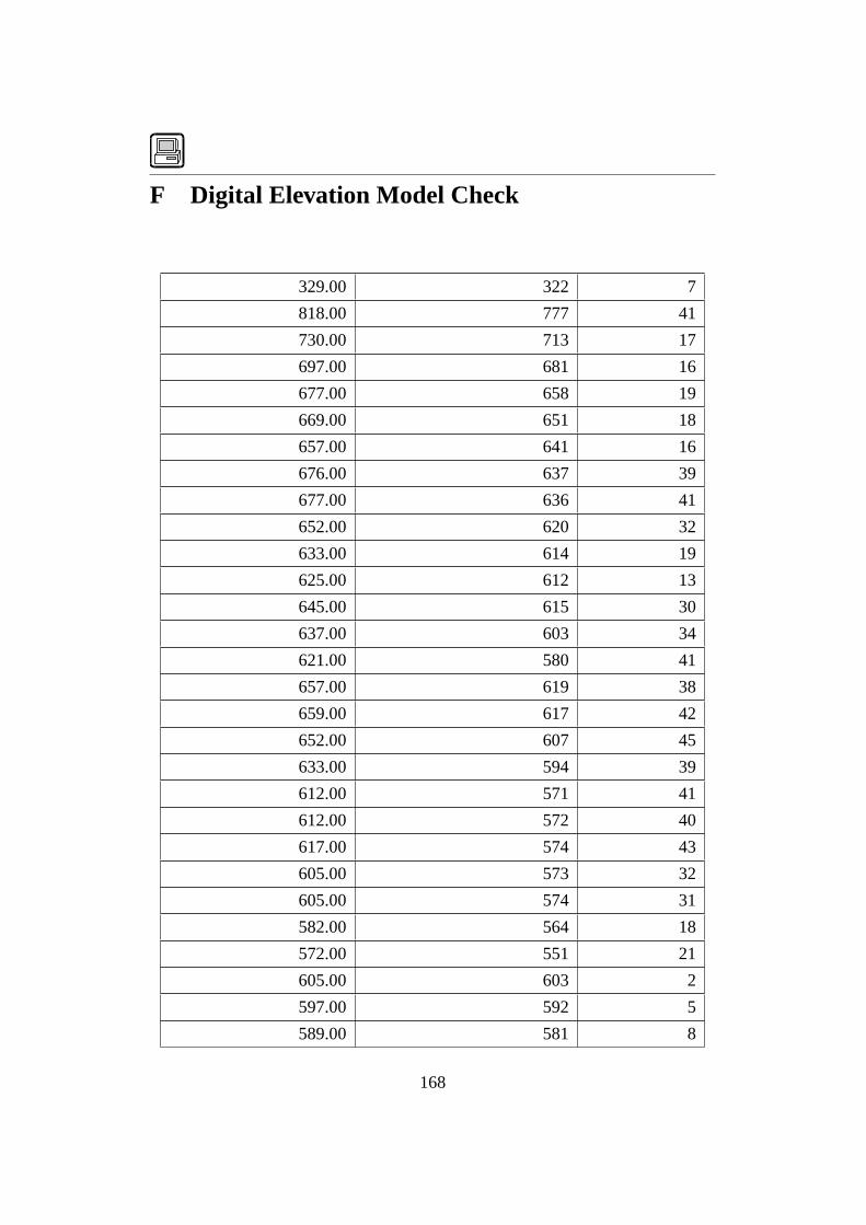
F Digital Elevation Model Check
329.00 322 7
818.00 777 41
730.00 713 17
697.00 681 16
677.00 658 19
669.00 651 18
657.00 641 16
676.00 637 39
677.00 636 41
652.00 620 32
633.00 614 19
625.00 612 13
645.00 615 30
637.00 603 34
621.00 580 41
657.00 619 38
659.00 617 42
652.00 607 45
633.00 594 39
612.00 571 41
612.00 572 40
617.00 574 43
605.00 573 32
605.00 574 31
582.00 564 18
572.00 551 21
605.00 603 2
597.00 592 5
589.00 581 8
168

DEM Elevation in m aSL Altimeter Elevation in m aSL Difference in m
575.00 571 4
581.00 564 17
568.00 551 17
553.00 521 32
568.00 563 5
572.00 578 6
582.00 582 0
577.00 550 27
584.00 559 25
597.00 558 39
640.00 617 23
640.00 614 26
642.00 603 39
625.00 590 35
625.00 600 25
635.00 612 23
654.00 638 16
678.00 660 18
624.00 588 36
620.00 594 26
596.00 565 31
595.00 605 10
570.00 563 7
565.00 548 17
590.00 556 34
590.00 563 27
580.00 567 13
554.00 532 22
542.00 527 15
560.00 540 20
566.00 527 39
169

DEM Elevation in m aSL Altimeter Elevation in m aSL Difference in m
635.00 612 23
639.00 598 41
602.00 560 42
612.00 609 3
635.00 612 23
610.00 607 3
605.00 603 2
610.00 582 28
608.00 570 38
615.00 572 43
596.00 558 38
580.00 578 2
575.00 553 22
560.00 533 27
540.00 523 17
550.00 529 21
565.00 520 45
595.00 549 46
550.00 550 0
550.00 512 38
360.00 316 44
644.00 606 38
462.00 458 4
413.00 447 34
372.00 398 26
327.00 320 7
332.00 302 30
170

G Logging Results
171

H Judayta Pumping Station
172

I Al Koura Water Supply Network
173

J Judayta Spot Heights
174

K Judayta Logger Locations
175

L Hydraulic Analysis Model Judayta
176