designing distributed systems for intermittent powernksharma/thesis/thesis.pdf · designing...

DESIGNING DISTRIBUTED SYSTEMS FOR INTERMITTENTPOWER

A Dissertation Presented

by

NAVIN KUMAR SHARMA

Submitted to the Graduate School of theUniversity of Massachusetts Amherst in partial fulfillment

of the requirements for the degree of

DOCTOR OF PHILOSOPHY

May 2013

Computer Science


A Dissertation Presented

by

NAVIN KUMAR SHARMA

Approved as to style and content by:

Prashant Shenoy, Chair

Deepak Ganesan, Member

James Kurose, Member

Michael Zink, Member

Lori A. Clarke, Department ChairComputer Science

To my parents and my brothers, Santosh and Mukesh.

ACKNOWLEDGMENTS

I would first like this opportunity to thank my PhD advisor Prof. Prashant Shenoywithout whose guidance I would not have received a doctorate. Over the years he hashelped me transition from a system engineer to a system researcher who combines strongdevelopment skills with research skills to build real systems that impact real people. It wasdue to his guidance and mentoring skills that I have enjoyed my academic career more thanmy professional career.

Next, I am deeply indebted to Prof. David Irwin who has been my (unofficial) co-advisor for the last five years. His guidance and invaluable comments have led me tofinish my PhD work in a timely fashion. I would also like to thank my other committeemembers, Prof. Deepak Ganesan, Prof. James Kurose, and Prof. Michael Zink, who haveconstantly given me valuable inputs on various research projects, that led to many highquality publications.

I would like to thank my colleagues Jeremy Gummeson, Pranshu Sharma, Sean Barker,and Dilip Krishnappa with whom I have worked on several projects which form part ofthis dissertation. I am also grateful to the other members of the LASS group, particularlyUpendra Sharma and Rahul Singh, with whom I have spent countless hours discussinga range of topics from research to politics. My time in Amherst was made even moreenjoyable by the incredible group of friends I developed over the years. Specifically, I amgrateful to Ameet Shetty, Anindya Misra, JP Mahalik, Supratim Mukherjee, and VimalMathew, for always being ready to help whenever I needed any.

My sincere thanks to Tyler Trafford for his assistance in managing the machines thatwere central to my doctoral work. Many thanks to the CSCF staff who helped me overcomeseveral technical problems that I faced while developing research prototypes for my thesis.I am also indebted to Leeanne Leclerc for keeping my paperwork organized and on track,and to Karren Sacco for handling all administrative work; they have taken care of manynon-technical problems I had.

This journey would not have been started without the support and guidance of my un-dergraduate advisors – Prof. Arobinda Gupta, Prof. Rajarshi Roy, and Prof. ShamikSural – and my mentor D. D. Ganguly. They have always believed in me and inspired meto dream beyond my limitations. I am also fortunate to have worked with an awesomegroup of people before starting my PhD career, particularly my supervisor Rohit Shankarand colleagues Bharat Varma, Prasanth Radhakrishnan, and Rajesh Dharmalingam, whosefriendships I will always cherish.

Finally, I am obliged to my parents, my brothers Santosh Sharma and Mukesh Sharma,my sisters-in-law Nitu Sharma and Nupur Sinha, and my nephew Nitin Sharma, who haveinfluenced me the most and were always there to support and encourage me. They havebeen my source of strength. I dedicate this thesis to them.

v

ABSTRACT


MAY 2013

NAVIN KUMAR SHARMA

B.Tech., INDIAN INSTITUTE OF TECHNOLOGY KHARAGPUR INDIA

M.S., UNIVERSITY OF MASSACHUSETTS AMHERST

Ph.D., UNIVERSITY OF MASSACHUSETTS AMHERST

Directed by: Professor Prashant Shenoy

The increasing demand for computing infrastructure, such as data centers and storagesystems, has increased their energy footprint. As a result of this growth, computing infras-tructure today contribute 2-3% of the global carbon emissions. Furthermore, the energy-related costs have now become a significant fraction of the total cost of ownership (TCO)of a modern computing infrastructure. Hence, to reduce the financial and environmentalimpact of growing energy demands the design of eco-friendly green infrastructure has be-come an important societal need. This thesis focuses on designing distributed systems,primarily data centers and storage systems, to run on renewable energy sources such assolar and wind.

As renewables are intermittent in nature, accurate predictions of future energy is impor-tant for a distributed system to balance workload demand and energy supply, and optimizeits performance amid significant and frequent changes in both demand and supply. To accu-rately predict energy harvesting in all weather conditions, I develop two prediction modelsthat leverage weather forecasts to predict solar and wind energy harvesting. The first pre-diction model is an empirical model that uses sky cover forecast and wind speed forecastto predict solar energy and wind energy, respectively, in the future. The second predictionmodel is a machine learning based model that uses statistical power of machine learningtechniques to give better predictions of solar energy harvesting than the empirical model.

To regulate the energy footprint of a server I propose a new energy abstraction, calledBlink, that applies duty cycle to the server to cap power consumption to supply. I also pro-

vi

pose several blinking policies to coordinate blinking across servers to regulate cluster-widepower consumption with changes in the available power. Further, I show that a real-worldapplication can be redesigned, with modest complexity, to perform well on intermittentpower.

To extend the applicability of blinking beyond an in-memory cache server I use theblinking abstraction to design two different distributed systems – (a) Distributed File Sys-tem, and (b) Multimedia Cache – for intermittent power. I propose several design tech-niques, including a staggered blinking policy and power-balanced data layout, to optimizethe performance of these systems under intermittent power scenarios. Additionally, I ex-periment with three unmodified real-world applications – (a) Memcache, (b) MapReduce,and (c) Search Engine – to test the practicality of our blink-aware file system. Our resultsshow that real-world applications can perform reasonably well for real workloads in spite ofsignificant and frequent variations in power supply. Finally, I use a real WiMAX testbed todemonstrate that our blink-aware multimedia cache can significantly save bandwidth usageof cell towers while providing good performance under intermittent power constraints.

vii

TABLE OF CONTENTS

Page

ACKNOWLEDGMENTS . . . . . . . . . . . . . . . . . . . . . . . . . . . . . . . . . . . . . . . . . . . . . . . . . . . v

ABSTRACT . . . . . . . . . . . . . . . . . . . . . . . . . . . . . . . . . . . . . . . . . . . . . . . . . . . . . . . . . . . . . . vi

LIST OF TABLES . . . . . . . . . . . . . . . . . . . . . . . . . . . . . . . . . . . . . . . . . . . . . . . . . . . . . . . . . xi

LIST OF FIGURES . . . . . . . . . . . . . . . . . . . . . . . . . . . . . . . . . . . . . . . . . . . . . . . . . . . . . . . xii

CHAPTER

1. INTRODUCTION . . . . . . . . . . . . . . . . . . . . . . . . . . . . . . . . . . . . . . . . . . . . . . . . . . . . . . 11.1 Background and Motivation . . . . . . . . . . . . . . . . . . . . . . . . . . . . . . . . . . . . . . . . . . . 11.2 Thesis Contributions . . . . . . . . . . . . . . . . . . . . . . . . . . . . . . . . . . . . . . . . . . . . . . . . . 3

1.2.1 Energy Harvesting Prediction . . . . . . . . . . . . . . . . . . . . . . . . . . . . . . . . . . . 41.2.2 Energy Footprint Regulation . . . . . . . . . . . . . . . . . . . . . . . . . . . . . . . . . . . 51.2.3 Performance Optimization . . . . . . . . . . . . . . . . . . . . . . . . . . . . . . . . . . . . . 6

1.3 Thesis Outline . . . . . . . . . . . . . . . . . . . . . . . . . . . . . . . . . . . . . . . . . . . . . . . . . . . . . . 6

2. BACKGROUND AND RELATED WORK . . . . . . . . . . . . . . . . . . . . . . . . . . . . . . . . . 82.1 Energy Harvesting Prediction . . . . . . . . . . . . . . . . . . . . . . . . . . . . . . . . . . . . . . . . . 82.2 Power Management in Data Centers . . . . . . . . . . . . . . . . . . . . . . . . . . . . . . . . . . . . 82.3 Duty Cycling in Low-Power Devices . . . . . . . . . . . . . . . . . . . . . . . . . . . . . . . . . . 102.4 Distributed File Systems . . . . . . . . . . . . . . . . . . . . . . . . . . . . . . . . . . . . . . . . . . . . . 102.5 Multimedia Caches . . . . . . . . . . . . . . . . . . . . . . . . . . . . . . . . . . . . . . . . . . . . . . . . . 11

3. WEATHER FORECASTS BASED ENERGY HARVESTINGPREDICTION MODELS . . . . . . . . . . . . . . . . . . . . . . . . . . . . . . . . . . . . . . . . . . . . 12

3.1 Background and Motivation . . . . . . . . . . . . . . . . . . . . . . . . . . . . . . . . . . . . . . . . . . 123.2 The Case for Using Forecasts . . . . . . . . . . . . . . . . . . . . . . . . . . . . . . . . . . . . . . . . 143.3 Forecast→ Energy Model . . . . . . . . . . . . . . . . . . . . . . . . . . . . . . . . . . . . . . . . . . . 17

3.3.1 Sky Condition→ Solar Power Model . . . . . . . . . . . . . . . . . . . . . . . . . . . 183.3.1.1 Computing Solar Power From Solar Radiation . . . . . . . . . . . 183.3.1.2 Computing the Maximum Possible Solar Power . . . . . . . . . . 193.3.1.3 Solar Model . . . . . . . . . . . . . . . . . . . . . . . . . . . . . . . . . . . . . . . 20

viii

3.3.2 Wind Speed→Wind Power Model . . . . . . . . . . . . . . . . . . . . . . . . . . . . . 203.3.3 Compensating for Forecast Errors . . . . . . . . . . . . . . . . . . . . . . . . . . . . . . 21

3.4 Comparison with PPF Variants . . . . . . . . . . . . . . . . . . . . . . . . . . . . . . . . . . . . . . . 213.5 Related Work . . . . . . . . . . . . . . . . . . . . . . . . . . . . . . . . . . . . . . . . . . . . . . . . . . . . . . 243.6 Conclusion . . . . . . . . . . . . . . . . . . . . . . . . . . . . . . . . . . . . . . . . . . . . . . . . . . . . . . . . 24

4. MACHINE LEARNING MODEL FOR SOLAR ENERGY HARVESTINGPREDICTION . . . . . . . . . . . . . . . . . . . . . . . . . . . . . . . . . . . . . . . . . . . . . . . . . . . . . . 25

4.1 Background and Motivation . . . . . . . . . . . . . . . . . . . . . . . . . . . . . . . . . . . . . . . . . . 254.2 Data Analysis . . . . . . . . . . . . . . . . . . . . . . . . . . . . . . . . . . . . . . . . . . . . . . . . . . . . . . 264.3 Prediction Models . . . . . . . . . . . . . . . . . . . . . . . . . . . . . . . . . . . . . . . . . . . . . . . . . . 29

4.3.1 Linear Least Squares Regression . . . . . . . . . . . . . . . . . . . . . . . . . . . . . . . 304.3.2 Support Vector Machines . . . . . . . . . . . . . . . . . . . . . . . . . . . . . . . . . . . . . 314.3.3 Eliminating Redundant Information . . . . . . . . . . . . . . . . . . . . . . . . . . . . 334.3.4 Comparing with Existing Models . . . . . . . . . . . . . . . . . . . . . . . . . . . . . . 33

4.4 Conclusion . . . . . . . . . . . . . . . . . . . . . . . . . . . . . . . . . . . . . . . . . . . . . . . . . . . . . . . . 34

5. MANAGING SERVER CLUSTERS ON INTERMITTENT POWER . . . . . . . . 355.1 Background and Motivation . . . . . . . . . . . . . . . . . . . . . . . . . . . . . . . . . . . . . . . . . . 35

5.1.1 Example: BlinkCache . . . . . . . . . . . . . . . . . . . . . . . . . . . . . . . . . . . . . . . . 365.1.2 Contributions . . . . . . . . . . . . . . . . . . . . . . . . . . . . . . . . . . . . . . . . . . . . . . . 37

5.2 Blink: Rationale and Overview . . . . . . . . . . . . . . . . . . . . . . . . . . . . . . . . . . . . . . . 385.3 Blink Prototype . . . . . . . . . . . . . . . . . . . . . . . . . . . . . . . . . . . . . . . . . . . . . . . . . . . . 41

5.3.1 Blink Hardware Platform . . . . . . . . . . . . . . . . . . . . . . . . . . . . . . . . . . . . . 425.3.1.1 Energy Sources . . . . . . . . . . . . . . . . . . . . . . . . . . . . . . . . . . . . . 425.3.1.2 Low-power Server Cluster . . . . . . . . . . . . . . . . . . . . . . . . . . . . 43

5.3.2 Blink Software Architecture . . . . . . . . . . . . . . . . . . . . . . . . . . . . . . . . . . . 445.4 Blinking Memcached . . . . . . . . . . . . . . . . . . . . . . . . . . . . . . . . . . . . . . . . . . . . . . . 45

5.4.1 Memcached Overview . . . . . . . . . . . . . . . . . . . . . . . . . . . . . . . . . . . . . . . . 455.4.2 Access Patterns and Performance Metrics . . . . . . . . . . . . . . . . . . . . . . . 465.4.3 BlinkCache Design Alternatives . . . . . . . . . . . . . . . . . . . . . . . . . . . . . . . 47

5.4.3.1 Activation Policy . . . . . . . . . . . . . . . . . . . . . . . . . . . . . . . . . . . 485.4.3.2 Synchronous Policy . . . . . . . . . . . . . . . . . . . . . . . . . . . . . . . . . 505.4.3.3 Load-Proportional Policy . . . . . . . . . . . . . . . . . . . . . . . . . . . . 51

5.4.4 Summary . . . . . . . . . . . . . . . . . . . . . . . . . . . . . . . . . . . . . . . . . . . . . . . . . . 525.5 Implementation and Evaluation . . . . . . . . . . . . . . . . . . . . . . . . . . . . . . . . . . . . . . . 52

5.5.1 Benchmarks . . . . . . . . . . . . . . . . . . . . . . . . . . . . . . . . . . . . . . . . . . . . . . . . 535.5.1.1 Activation Blinking and Thrashing . . . . . . . . . . . . . . . . . . . . . 555.5.1.2 Synchronous Blinking and Fairness . . . . . . . . . . . . . . . . . . . . 565.5.1.3 Balancing Performance and Fairness . . . . . . . . . . . . . . . . . . . 57

5.5.2 Case Study: Tag Clouds in GlassFish . . . . . . . . . . . . . . . . . . . . . . . . . . . 595.6 Related Work . . . . . . . . . . . . . . . . . . . . . . . . . . . . . . . . . . . . . . . . . . . . . . . . . . . . . . 605.7 Conclusion . . . . . . . . . . . . . . . . . . . . . . . . . . . . . . . . . . . . . . . . . . . . . . . . . . . . . . . . 61

ix

6. DISTRIBUTED FILE SYSTEM FOR INTERMITTENT POWER . . . . . . . . . . 636.1 Background and Motivation . . . . . . . . . . . . . . . . . . . . . . . . . . . . . . . . . . . . . . . . . . 636.2 DFSs and Intermittent Power . . . . . . . . . . . . . . . . . . . . . . . . . . . . . . . . . . . . . . . . . 66

6.2.1 Energy-Proportional DFSs . . . . . . . . . . . . . . . . . . . . . . . . . . . . . . . . . . . . 676.2.2 Migration-based Approach . . . . . . . . . . . . . . . . . . . . . . . . . . . . . . . . . . . . 686.2.3 Equal-Work Approach . . . . . . . . . . . . . . . . . . . . . . . . . . . . . . . . . . . . . . . 69

6.3 Applying Blinking to DFSs . . . . . . . . . . . . . . . . . . . . . . . . . . . . . . . . . . . . . . . . . . 706.4 BlinkFS Design . . . . . . . . . . . . . . . . . . . . . . . . . . . . . . . . . . . . . . . . . . . . . . . . . . . . 70

6.4.1 Reading and Writing Files . . . . . . . . . . . . . . . . . . . . . . . . . . . . . . . . . . . . 726.4.2 Reducing the Latency Penalty . . . . . . . . . . . . . . . . . . . . . . . . . . . . . . . . . 74

6.5 Implementation . . . . . . . . . . . . . . . . . . . . . . . . . . . . . . . . . . . . . . . . . . . . . . . . . . . . 766.6 Evaluation . . . . . . . . . . . . . . . . . . . . . . . . . . . . . . . . . . . . . . . . . . . . . . . . . . . . . . . . 79

6.6.1 Benchmarks . . . . . . . . . . . . . . . . . . . . . . . . . . . . . . . . . . . . . . . . . . . . . . . . 796.6.2 Case Studies . . . . . . . . . . . . . . . . . . . . . . . . . . . . . . . . . . . . . . . . . . . . . . . . 81

6.7 Conclusion . . . . . . . . . . . . . . . . . . . . . . . . . . . . . . . . . . . . . . . . . . . . . . . . . . . . . . . . 84

7. MULTIMEDIA CACHE FOR INTERMITTENT POWER . . . . . . . . . . . . . . . . . 857.1 Background and Motivation . . . . . . . . . . . . . . . . . . . . . . . . . . . . . . . . . . . . . . . . . . 857.2 Cache and Intermittent Power . . . . . . . . . . . . . . . . . . . . . . . . . . . . . . . . . . . . . . . . 877.3 GreenCache Feasibility: Trace Analysis . . . . . . . . . . . . . . . . . . . . . . . . . . . . . . . . 907.4 GreenCache Design . . . . . . . . . . . . . . . . . . . . . . . . . . . . . . . . . . . . . . . . . . . . . . . . 92

7.4.1 Minimizing Bandwidth Cost . . . . . . . . . . . . . . . . . . . . . . . . . . . . . . . . . . 937.4.2 Reducing Buffering Time . . . . . . . . . . . . . . . . . . . . . . . . . . . . . . . . . . . . . 94

7.4.2.1 Staggered Load-Proportional Blinking . . . . . . . . . . . . . . . . . 947.4.2.2 Prefetching Recommended Videos . . . . . . . . . . . . . . . . . . . . . 95

7.5 GreenCache Implementation . . . . . . . . . . . . . . . . . . . . . . . . . . . . . . . . . . . . . . . . . 967.6 Experimental Evaluation . . . . . . . . . . . . . . . . . . . . . . . . . . . . . . . . . . . . . . . . . . . . 98

7.6.1 Benchmarks . . . . . . . . . . . . . . . . . . . . . . . . . . . . . . . . . . . . . . . . . . . . . . . . 987.6.2 Staggered load-proportional blinking . . . . . . . . . . . . . . . . . . . . . . . . . . 1007.6.3 Case study . . . . . . . . . . . . . . . . . . . . . . . . . . . . . . . . . . . . . . . . . . . . . . . . 102

7.7 Related Work . . . . . . . . . . . . . . . . . . . . . . . . . . . . . . . . . . . . . . . . . . . . . . . . . . . . . 1027.8 Conclusion . . . . . . . . . . . . . . . . . . . . . . . . . . . . . . . . . . . . . . . . . . . . . . . . . . . . . . . 103

8. SUMMARY AND FUTURE WORK . . . . . . . . . . . . . . . . . . . . . . . . . . . . . . . . . . . . 1048.1 Thesis Summary . . . . . . . . . . . . . . . . . . . . . . . . . . . . . . . . . . . . . . . . . . . . . . . . . . 1048.2 Future Work . . . . . . . . . . . . . . . . . . . . . . . . . . . . . . . . . . . . . . . . . . . . . . . . . . . . . . 105

BIBLIOGRAPHY . . . . . . . . . . . . . . . . . . . . . . . . . . . . . . . . . . . . . . . . . . . . . . . . . . . . . . . . 107

x

LIST OF TABLES

Table Page

1.1 Challenges with existing green computing techniques for data centers. . . . . . . . 3

3.1 Values for a, b, and c in our quadratic solar power model, which is afunction of the time of day for each month of the year. . . . . . . . . . . . . . . . . . 20

4.1 Correlation matrix showing correlation between different forecastparameters. . . . . . . . . . . . . . . . . . . . . . . . . . . . . . . . . . . . . . . . . . . . . . . . . . . . . . 29

5.1 Latencies for several desktop and laptop models to perform a complete S3cycle (suspend and resume). Data from both [35] and our ownmeasurements of Blink’s OLPC-X0. . . . . . . . . . . . . . . . . . . . . . . . . . . . . . . . 39

5.2 Blink APIs for setting per-node blinking schedules. . . . . . . . . . . . . . . . . . . . . . . 44

5.3 Blink’s measurement APIs that applications use to inform their blinkingdecisions. . . . . . . . . . . . . . . . . . . . . . . . . . . . . . . . . . . . . . . . . . . . . . . . . . . . . . . 44

5.4 Summary of the best policy for a given performance metric and workloadcombination. . . . . . . . . . . . . . . . . . . . . . . . . . . . . . . . . . . . . . . . . . . . . . . . . . . . 52

6.1 POSIX-compliant API for BlinkFS . . . . . . . . . . . . . . . . . . . . . . . . . . . . . . . . . . . . 77

6.2 Standard deviation and 90th percentile latency. . . . . . . . . . . . . . . . . . . . . . . . . . . 80

7.1 Standard deviation, 90th percentile, and average buffering time. . . . . . . . . . . . . 98

xi

LIST OF FIGURES

Figure Page

1.1 System overview . . . . . . . . . . . . . . . . . . . . . . . . . . . . . . . . . . . . . . . . . . . . . . . . . . . . 4

3.1 Power generated during a 12 day period in October, 2009 from our solarpanel (a) and wind turbine (b). . . . . . . . . . . . . . . . . . . . . . . . . . . . . . . . . . . . . . 13

3.2 The error in sky condition (a) and wind speed (b) when using the past topredict the future for different time intervals in 2008 at 1 hour and 5minute granularities, respectively, for Amherst, Massachusetts. . . . . . . . . . 14

3.3 RMSE between the observed sky condition and wind speed and thosepredicted by NWS forecasts from 3 hours to 72 hours in the future. . . . . . . 17

3.4 Relationship between the solar radiation our weather station observes andthe power generated by our solar panel. . . . . . . . . . . . . . . . . . . . . . . . . . . . . . 17

3.5 Profile for solar power harvested on clear and sunny days in January, May,and September, and the quadratic functions f(x), g(x), and h(x) we fitto each profile, respectively. . . . . . . . . . . . . . . . . . . . . . . . . . . . . . . . . . . . . . . . 19

3.6 Power output from our wind turbine and the power output predicted by ourwind power model over the first 3 weeks of October. The graph showsthe rated power curves from the wind turbines manual for steady andturbulent wind, as well as our fitted curve. . . . . . . . . . . . . . . . . . . . . . . . . . . . 21

3.7 Power output from our solar panel and the power output predicted bydifferent prediction models over the first 3 weeks of October, 2009. . . . . . . 22

3.8 Power output from our wind turbine and the power output predicted bydifferent prediction models over the first 3 weeks of October, 2009. . . . . . . 23

4.1 Solar intensity shows seasonal variation with days of a year, althoughdaily weather conditions also have a significant impact. . . . . . . . . . . . . . . . . 27

4.2 Solar intensity and wind speed show little correlation (a). Solar intensityshows some correlation with temperature at high temperatures (b) andwith dew point at high dew points (c). . . . . . . . . . . . . . . . . . . . . . . . . . . . . . . 27

xii

4.3 Solar intensity generally decreases with increasing values of sky cover (a),relative humidity (b), and precipitation potential (c). . . . . . . . . . . . . . . . . . . 28

4.4 Relative humidity (a) and precipitation % (b) positively correlate with skycover. Relative humidity also increases with increasing precipitation% (c). . . . . . . . . . . . . . . . . . . . . . . . . . . . . . . . . . . . . . . . . . . . . . . . . . . . . . . . . . 29

4.5 Observed and predicted solar intensity using linear least squaresregression for September and October 2010. . . . . . . . . . . . . . . . . . . . . . . . . . 31

4.6 Observed and predicted solar intensity, using SVM regression with anRBF kernel, for the months of September and October 2010. . . . . . . . . . . . 32

4.7 Observed and predicted solar intensity, using three different predictiontechniques — (a) SVM-RBF kernel with 4 dimensions, (b) cloudycomputing model using sky condition forecast, (c) past predicts futureprediction model — for the months of September and October2010. . . . . . . . . . . . . . . . . . . . . . . . . . . . . . . . . . . . . . . . . . . . . . . . . . . . . . . . . . . 32

5.1 The popularity of web data often exhibits a long heavy tail of equallyunpopular objects. This graph ranks the popularity of Facebook grouppages by their number of fans. . . . . . . . . . . . . . . . . . . . . . . . . . . . . . . . . . . . . . 37

5.2 Hardware architecture of the Blink prototype. . . . . . . . . . . . . . . . . . . . . . . . . . . . 41

5.3 Empirically-measured battery capacity as a function of voltage for ourdeep-cycle battery. We consider the battery empty below 12V, sinceusing it beyond this level will reduce its lifetime. . . . . . . . . . . . . . . . . . . . . . 43

5.4 The popularity rank, by number of fans, for all 20 million public grouppages on Facebook follows a Zipf-like distribution with α = 0.6. . . . . . . . . 46

5.5 To explicitly control the mapping of keys to servers, we interposealways-active request proxies between memcached clients and servers.The proxies are able to monitor per-key hit rates and migrate similarlypopular objects to the same nodes. . . . . . . . . . . . . . . . . . . . . . . . . . . . . . . . . . 49

5.6 Graphical depiction of a static/dynamic activation blinking policy (a), anactivation blinking policy with key migration (b), and a synchronousblinking policy (c). . . . . . . . . . . . . . . . . . . . . . . . . . . . . . . . . . . . . . . . . . . . . . . 51

xiii

5.7 The near 2 second latency to transition into and out of S3 in our prototypediscourages blinking intervals shorter than roughly 40 seconds. With a50% duty cycle we expect to operate at 50% full power, but with ablink interval of less than 10 seconds we operate near 100% fullpower. . . . . . . . . . . . . . . . . . . . . . . . . . . . . . . . . . . . . . . . . . . . . . . . . . . . . . . . . . 54

5.8 Maximum throughput (a) and latency (b) for a dedicated memcachedserver, our memcached proxy, and a MySQL server. Our proxyimposes only a modest overhead compared with a dedicatedmemcached server. . . . . . . . . . . . . . . . . . . . . . . . . . . . . . . . . . . . . . . . . . . . . . . 54

5.9 Under constant power for a Zipf popularity distribution, the dynamicvariant of the activation policy performs better than the static variantas power decreases. However, the activation policy with key migrationoutperforms the other variants. . . . . . . . . . . . . . . . . . . . . . . . . . . . . . . . . . . . . 55

5.10 Under oscillating power for a Zipf popularity distribution, the staticvariant of the activation policy performs better than the dynamicvariant as the oscillation increases. Again, the activation policy withkey migration outperforms the other variants. . . . . . . . . . . . . . . . . . . . . . . . . 56

5.11 For a uniform popularity distribution, both the synchronous policy and thedynamic variant of the activation policy are significantly more fair, i.e.,lower standard deviation of average per-object latency, than theactivation policy with key migration. . . . . . . . . . . . . . . . . . . . . . . . . . . . . . . . 57

5.12 For a uniform popularity distribution, the synchronous policy and theactivation policy with key migration achieve a similar hit rate underdifferent power levels. Both policies achieve a better hit rate than thedynamic variant of the activation policy. . . . . . . . . . . . . . . . . . . . . . . . . . . . . . 57

5.13 The load-proportional policy is more fair to the unpopular objects, i.e.bottom 80% in popularity, than the activation policy with keymigration for Zip popularity distributions, especially in low-powerscenarios. . . . . . . . . . . . . . . . . . . . . . . . . . . . . . . . . . . . . . . . . . . . . . . . . . . . . . . 58

5.14 The load-proportional policy has a slightly lower hit rate than theactivation policy with key migration. . . . . . . . . . . . . . . . . . . . . . . . . . . . . . . . 58

5.15 As S3 transition overhead increases, the hit rate from the load-proportionalpolicy decreases relative to the activation policy with key migration fora Zipf distribution at a moderate power level. . . . . . . . . . . . . . . . . . . . . . . . . 59

5.16 Power signal from a combined wind/solar deployment (a) and averagepage load latency for that power signal (b). . . . . . . . . . . . . . . . . . . . . . . . . . . 59

xiv

6.1 Electricity prices vary every five minutes to an hour in wholesale markets,resulting in the power available for a fixed monetary budget varyingconsiderably over time. . . . . . . . . . . . . . . . . . . . . . . . . . . . . . . . . . . . . . . . . . . . 64

6.2 Inaccessible data rises with the fraction of inactive nodes using a randomreplica placement policy. . . . . . . . . . . . . . . . . . . . . . . . . . . . . . . . . . . . . . . . . . 68

6.3 Simple example using a migration-based approach (a) and blinking (b) todeal with power variations. . . . . . . . . . . . . . . . . . . . . . . . . . . . . . . . . . . . . . . . . 69

6.4 BlinkFS Architecture . . . . . . . . . . . . . . . . . . . . . . . . . . . . . . . . . . . . . . . . . . . . . . . 71

6.5 Combining staggered blinking (a) with a power-balanced data layout (b)maximizes block availability. . . . . . . . . . . . . . . . . . . . . . . . . . . . . . . . . . . . . . . 72

6.6 BlinkFS hardware prototype. . . . . . . . . . . . . . . . . . . . . . . . . . . . . . . . . . . . . . . . . . 78

6.7 Maximum sequential read/write throughput for different block sizes withand without the proxy. . . . . . . . . . . . . . . . . . . . . . . . . . . . . . . . . . . . . . . . . . . . . 78

6.8 Read and write latency in our BlinkFS prototype at different power levelsand block replication factors. . . . . . . . . . . . . . . . . . . . . . . . . . . . . . . . . . . . . . . 79

6.9 Maximum possible throughput in our BlinkFS prototype for differentnumber of block servers. . . . . . . . . . . . . . . . . . . . . . . . . . . . . . . . . . . . . . . . . . . 81

6.10 BlinkFS performs well as power oscillation increases. . . . . . . . . . . . . . . . . . . . . 82

6.11 MapReduce completion time at steady power levels and using ourcombined wind/solar power trace. . . . . . . . . . . . . . . . . . . . . . . . . . . . . . . . . . . 82

6.12 MemcacheDB average latency at steady power levels and using ourcombined wind/solar power signal. . . . . . . . . . . . . . . . . . . . . . . . . . . . . . . . . . 83

6.13 Search engine query rate with price signal from 5-minute spot price inNew England market. . . . . . . . . . . . . . . . . . . . . . . . . . . . . . . . . . . . . . . . . . . . . 84

7.1 Solar and wind energy harvesting from our solar panel and wind turbinedeployment on three consecutive days in Sep 2009. . . . . . . . . . . . . . . . . . . . 88

7.2 The top part of the figure shows a potential streaming schedule for ablinking node while the bottom half shows the smooth play out with isachieved with the aid of a client-side buffer. . . . . . . . . . . . . . . . . . . . . . . . . . 90

7.3 Video Popularity (100 out of 105339) . . . . . . . . . . . . . . . . . . . . . . . . . . . . . . . . . . 91

xv

7.4 Related Video Position Analysis . . . . . . . . . . . . . . . . . . . . . . . . . . . . . . . . . . . . . . 92

7.5 Video Switching Time Analysis . . . . . . . . . . . . . . . . . . . . . . . . . . . . . . . . . . . . . . . 92

7.6 GreenCache Architecture. . . . . . . . . . . . . . . . . . . . . . . . . . . . . . . . . . . . . . . . . . . . 93

7.7 Staggered load-proportional blinking. . . . . . . . . . . . . . . . . . . . . . . . . . . . . . . . . . . 93

7.8 Hardware Prototype. . . . . . . . . . . . . . . . . . . . . . . . . . . . . . . . . . . . . . . . . . . . . . . . . 96

7.9 Both bandwidth usage and buffering time reduce with increasing cachesize. . . . . . . . . . . . . . . . . . . . . . . . . . . . . . . . . . . . . . . . . . . . . . . . . . . . . . . . . . . . 99

7.10 Video chunking reduces both bandwidth usage and buffering time. . . . . . . . . . 99

7.11 Buffering time at various steady and oscillating power levels. . . . . . . . . . . . . . 100

7.12 Buffering time decreases as the number of prefetched videos (first chunkonly) from related lists increases. . . . . . . . . . . . . . . . . . . . . . . . . . . . . . . . . . 100

7.13 Buffering time at various power levels for our combined solar/wind powertrace. . . . . . . . . . . . . . . . . . . . . . . . . . . . . . . . . . . . . . . . . . . . . . . . . . . . . . . . . . 102

xvi

CHAPTER 1

INTRODUCTION

As distributed systems, such as data centers and storage systems, are growing in num-bers and sizes the energy demands of these systems are also growing. The growing energydemands of distributed systems lead to burning more fossil fuels, which has long-term fi-nancial and environmental impact on our society. Reducing dependency on dirty fossilfuels by leveraging renewables to power distributed systems has become an important soci-etal need. This thesis addresses challenges associated with running distributed systems onrenewables, or intermittent power in general, and presents how distributed systems can bedesigned to operate completely off renewables while performing well at all power levels.

1.1 Background and Motivation

As computing infrastructure today contribute a significant fraction of the global carbonemissions, both industry and the research community are giving serious consideration onreducing the energy footprint of distributed systems. One obvious way to reduce the energyfootprint of distributed systems is to make them energy-proportional and more energy-efficient. In addition, one could also use a combination of renewables, such as solar andwind, and fossil fuels to power distributed systems, and focus on designing techniques tocompletely run the distributed systems off the renewables. The benefits of using renewablesare twofold. First, renewables are eco-friendly and don’t have any adverse environmentalimpact. Second, with increasing research attention on designing more sophisticated andenergy-efficient conversion technologies to generate electricity from renewables, in thefuture, the cost of renewable energy is likely to become cheaper than that of grid energy.

Prior research assumes that data centers have an unlimited supply of power, and focuseslargely on optimizing applications to use less energy without impacting performance. Onesuch approach is to consolidate loads on a small number of servers, e.g., using requestredirection or VM migration, and deactivate the remaining servers during off-peak hours.Since many applications, such as MapReduce, maintain distributed states, this approachnecessitates the migration of states before deactivating the servers, which might becomeprohibitively expensive in a typical data center.

Another approach for reducing energy consumption in data centers is to use a heteroge-nous set of nodes – low-power nodes along with high-power nodes [35, 36, 49]. Thesetechniques maintain a set of always-on low-power nodes to coexist with a set of high-powernodes, which are sent to a low-power state during idle periods or off-peak hours. The low-power nodes maintain active connections and provide basic services, such as responding toping requests, ICMP and ARP packets, etc., and wake up the high-power nodes on demand.

1

Though these approaches reduce the idle power waste, a significant energy saving mightbe hard to achieve if idle periods are not long enough to compensate for state transitionoverheads of the high-power nodes. Unlike mobile devices, high-power servers take sev-eral seconds to sleep, and thus cannot sleep during short idle periods, which are frequentfor many applications [127].

In recent years, the research community has started looking into various ways of inte-grating renewables to partially power data centers, while still relying on grids to providethe backup power [48, 50, 53, 70, 111, 110, 109]. Increasing renewable penetration de-mands adaptation to a variable power supply. While these techniques try to maximize therenewable penetration without degrading application performance, they are not designed tohandle intermittent power constraints, such as significant and frequent variations in powersupply or a sustained low power scenario. In contrast, there has been little research onrunning data centers solely on renewables, and optimizing application performance for in-termittent power that fluctuates over time. The primary challenge with using renewablesis that they are intermittent in nature. Consequently, a system should be designed to han-dle significant and frequent changes in the available power. Moreover, simply designing asystem to operate on intermittent power would not suffice because the performance mightbe intolerable in many cases. For example, a storage system could spend hours migratingdata to prevent data loss when the available power drops down significantly (∼ 90%), andthus becoming inaccessible for a long duration. So, running distributed systems solely offrenewables would be practical only when they adapt to intermittency in the power supplywhile performing well in spite of significant and frequent variations in the available power.

Aforementioned techniques could also use a large energy storage, e.g., a large num-ber of battery arrays, to handle intermittent power constraints. But, accurate predictionsof workload demand and energy supply are required to smooth out the power supply. Ifpredictions are inaccurate or there is a mismatch between supply and demand predictions,even a large energy storage would not prevent intermittency in the power supply. Further,maintaining a large energy storage is unsustainable and prohibitively expensive. Design-ing systems for renewables, or intermittent power in general, requires a dramatic departurefrom reducing energy consumption in distributed systems running on uninterrupted powersupply. The former demands optimizing performance for given power supply, while thelatter focuses on minimizing energy consumption for given workload demands or perfor-mance SLAs.

The central theme of this thesis is to explore how distributed systems can handle ex-treme power constraints, ranging from very high fluctuations to very low power scenarios,while performing well at all power levels without any knowledge of future supply and de-mand. Since a large energy storage is unsustainable and prohibitively expensive to manage,this thesis focuses on designing systems that adapt to the power supply, i.e., instantly regu-late energy footprint to match energy demand with supply. As renewables are intermittentand workload demands vary independent of harvested energy, accurate energy predictionscan significantly improve the performance without requiring a large energy storage. Forexample, a storage system could perform costly data migration in advance, when the poweris plenty, to keep data available when the power becomes scarce. Consequently, designingdistributed systems to operate off renewables, or intermittent power in general, consists ofthree major parts

2

Technique ChallengesActivation+Migration high migration overhead

inaccessible data at low powerHeterogenous nodes no energy savings during short idle periods

cannot handle intermittent power constraintsRenewables+Grid difficult to handle grid interruptions

cannot leverage variable electricity pricing

Table 1.1. Challenges with existing green computing techniques for data centers.

1. Energy Harvesting Prediction. Designing techniques to accurately predict futureenergy harvesting at short-to-medium time scales.

2. Energy Footprint Regulation. Designing hardware and software interface to regu-late energy footprint of distributed systems to cap power demand to power supply.

3. Performance Optimization. Designing techniques to maximize application perfor-mance at all power levels, and using future energy predictions for scheduling opera-tions to optimize overall performance of the system.

This thesis focuses primarily on data centers and storage systems as they are particularlywell-positioned to benefit from renewables, since unlike household and industrial loads,delay-tolerant batch workloads may permit performance degradation due to varying power.

1.2 Thesis Contributions

The fundamental thesis of this dissertation is to demonstrate that distributed systemscan be redesigned to run solely on renewables, or intermittent power in general, whileperforming well in spite of significant and frequent variations in the available power. Tothis end I have designed five key systems (Figure 1.1) which provide new algorithms andmechanisms to run distributed systems on intermittent power while maximizing applicationperformance at all power levels.

• Cloudy Computing. A novel technique to predict future solar and wind energy har-vesting from weather forecasts [94].

• ML Forecast. A powerful statistical model to predict solar energy harvesting usingmachine learning techniques [95].

• Blink. A new energy abstraction for regulating energy footprint of server clusters inorder to cap power consumption to the available power [93].

• BlinkFS. A distributed file system for intermittent power that avoids costly data mi-gration and maximizes I/O throughput and latency at all power levels [97].

3

Clody Computing ML Forecast Blink BlinkFS GreenCache

Energy Harvesting Prediction

Energy Footprint Regulation

Performance Optimization

Figure 1.1. The systems presented in this thesis to design distributed systems for intermit-tent power.

• GreenCache. A multimedia cache for intermittent power that minimizes bandwidthcost and access latency at all power levels [96].

1.2.1 Energy Harvesting Prediction

As discussed above, having knowledge of future energy harvesting is important formany distributed systems, running off renewables, to optimize application performance.Although many techniques exist to forecast future energy harvesting, they fail to predictdrastic changes in weather condition because their predictions are based on observationsin the past. While the past is accurate for both sufficiently short, i.e., seconds to minutes,and sufficiently long, i.e., months to years, time-scales, I show in Chapter 3 that predictionsbased on weather forecasts are more accurate at the medium time-scales, i.e., hours to days,relevant to a large class of distributed systems. Further, since forecasts from the NationalWeather Service (NWS) are based on complex mathematical models and observations fromsatellites and high-end radars, they tend to be reasonably accurate at the medium time-scales. Moreover, NWS forecasts can also predict drastic changes in weather condition,e.g., an incoming thunderstorm, which is not possible from predictions based on the past.

To improve the accuracy of energy harvesting prediction amid significant weather changes,I derive empirical models in Chapter 3 that leverage sky cover and wind speed forecast fromNWS to predict solar and wind energy harvesting, respectively, at short to medium-lengthintervals, i.e., hours to days. I also compare the efficiency of our prediction models withstate-of-the-art prediction techniques, and show that forecast-based models outperform theexisting techniques at short to medium time intervals.

As we expect, different weather parameters do not vary independently; rather they arecorrelated with each other. For example, if the temperature or dew point is high, then the so-lar intensity is likely to be high. But, understanding relationships between different weatherparameters and how they affect each other is not possible with simple empirical models, asdescribed above. In Chapter 4 I explore machine learning techniques to understand rela-tionships between different weather parameters and how they affect solar intensity. I findthat sky cover is not the only parameter which affects solar intensity; in fact, many otherparameters, such as humidity and precipitation, have strong correlation with solar intensity.To leverage all forecast parameters in solar energy prediction, I design machine learning

4

models that predict solar energy harvesting based on time and forecast of all weather pa-rameters. Our results show that SVM-based prediction models built using seven distinctweather forecast metrics outperform aforementioned forecast-based models by more than20% for our site.

1.2.2 Energy Footprint Regulation

Unlike grid energy, renewables are intermittent and can vary significantly and fre-quently without any warning. To operate completely off renewables distributed systemsmust be able to regulate their power consumption to match the available power. Designingenergy-proportional systems is challenging since many server components, including theCPU, memory, disk, motherboard, and power supply, now consume significant amounts ofpower. Thus, any power optimization that targets only a single component is not sufficient,since it reduces only a fraction of the total power consumption. For example, a modernserver that uses dynamic voltage and frequency scaling in the CPU at low utilization maystill operate at over 50% of its peak power. Thus, deactivating entire servers, includingmost of their components, remains the most effective technique for controlling energy con-sumption in server farms, especially at low power levels that necessitate operating serverswell below 50% peak power on average.

Simply varying the number of active nodes in response to changes in power has severaldrawbacks. First, application states might get lost if they are not transferred to active nodesbefore deactivating a set of nodes. Since power variations may be significant, it might notbe possible to transfer all states before deactivating the nodes. Second, if the availablepower is low (∼20% of peak power) consolidating all states on a small set of active nodesmight not be possible, since there might not be enough space to store the states. Third, statetransfer might be prohibitively expensive in a typical data center for even small variationsin power supply. For example, in a typical data center of 1000 nodes, where each nodestores 500 GB of data, deactivating 20% of the nodes, for 20% drop in the power, wouldlead to a 100 terabyte migration in the worst case. Migrating this data over a ten gigabitlink would take more than 10 hours, and prevent the data center from performing usefulwork.

Since long-term battery-based storage is prohibitively expensive, increasing renewableintegration requires closely matching power consumption to supply. For instant regulationof the energy footprint of a server cluster, in response to changes in the power supply, inChapter 5 I propose a new energy abstraction, called Blink, for gracefully handling inter-mittent power constraints. Blinking applies a duty cycle to servers that controls the fractionof time they are in the active state, e.g., by activating and deactivating them in succession, togracefully vary their energy footprint. Blinking generalizes the extremes of either keepinga server active (a 100% duty cycle) or inactive (a 0% duty cycle) by providing a spectrumof intermediate possibilities. I also propose a number of blinking policies to coordinateblinking of servers in a server cluster. I then design an application-independent platformfor developing and evaluating blinking applications, and use it to perform an in-depth studyof the effects of blinking on one particular application and power source: Memcached op-erating off renewable energy. Our results show that a real-world distributed application can

5

be redesigned, with modest overhead, to perform well on a server cluster operating solelyoff renewables.

1.2.3 Performance Optimization

As discussed above, Blink provides an application-independent abstraction for regu-lating energy footprint of a server. Further, blinking policies provide different ways ofcoordinating blinking of servers in a server cluster to regulate the energy footprint of thecluster. Blinking is a general abstraction for leveraging intermittent power in a wide rangeof applications. In Chapter 5 I discuss the applicability of the blinking abstraction foran in-memory distributed cache server. Another important application that can leveragethe blinking abstraction is a DFS (distributed file system). Since DFSs now serve as thefoundation for a wide range of data-intensive applications run in today’s data centers, de-signing a DFS optimized for intermittent power opens avenues for a number of applicationsto leverage the blinking abstraction without any modification. But designing such a DFSposes a significant research challenge, since periods of scarce power may render data in-accessible, while periods of plentiful power may require costly data layout adjustments toscale up I/O throughput.

Chapter 6 presents the design of BlinkFS, a distributed file system for intermittentpower, and shows how traditional file system operations can be redesigned to handle inter-mittency in the power supply. Further, I propose several techniques, including a staggeredblinking policy and power-balanced data layout, to optimize I/O throughput and latencyas power varies. To see the feasibility of BlinkFS for real-world applications I experimentwith three unmodified real-world applications – Memcache, MapReduce, Search Engine –on a small cluster of 10 Mac minis. Our results show that, with proposed optimizations,these real-world applications perform reasonably well in spite of significant and frequentvariations in power supply.

Unlike an in-memory key-value store, multimedia caches store data on persistent stor-age which become inaccessible at low power. Traditional multimedia caches assume un-limited supply of power and focus primarily on reducing backhaul bandwidth usage. Butrunning a multimedia cache on intermittent power warrants new approaches as a period oflow power makes cached contents unavailable, in which case reducing the bandwidth costincreases buffering time for end users. Thus, designing multimedia caches for intermit-tent power poses several new research challenges. In Chapter 7 I present the design of adistributed multimedia cache for intermittent power, called GreenCache, as well as severaloptimization techniques to provide multimedia caching while minimizing bandwidth costand latency at all power levels.

1.3 Thesis Outline

This thesis is structured as follows. Chapter 2 provides background on green comput-ing techniques in data centers and storage systems. Chapter 3 describes energy harvestingprediction models that leverage weather forecasts to predict solar and wind energy for anyforecast interval. This is followed in Chapter 4 with use of machine learning techniques to

6

design better prediction models for solar energy harvesting prediction. Chapter 5 presentsa hardware/software design to run server clusters on renewables, or intermittent power ingeneral. Chapter 6 presents the design of a blink-aware distributed file system to managestateful applications running concurrently on a data center running off renewables. Chap-ter 7 leverages the blinking abstraction from Chapter 5 to design a multimedia cache forintermittent power. Finally, Chapter 8 concludes the thesis and provides a brief overviewof future work.

7

CHAPTER 2

BACKGROUND AND RELATED WORK

This chapter provides a brief overview of energy harvesting prediction techniques andgreen computing techniques to reduce energy footprint of data centers and storage systems.Subsequent chapters also provide more detailed related work sections.

2.1 Energy Harvesting Prediction

Much of the prior work on energy harvesting assumes that past observed data providesa good indication of future energy harvesting. The simplest of these techniques is the past-predicts-future (PPF) model that predicts future energy harvesting as energy harvested inthe immediate past [9, 13]. Many variants of the PPF model have been proposed in re-cent years. Kansal et al. [9] maintain an exponentially weighted moving average (EWMA)for solar power to achieve energy-neutral operation in a system with elastic workload de-mands. The EWMA approach is a variant of PPF that adapts to seasonal variations in solarradiation. However, EWMA does not account for drastic changes in weather conditions,which are frequent in many areas. Noh et al. [15] use a historical model for solar radiationthat maintains an expectation for each time slot in a day based on the previous day’s solarradiation reading, but down-scales all future time-slots in a day by N% if it records a solarradiation reading N% less than expected.

The primary drawback of PPF techniques is that they fail to predict solar energy whenweather changes unpredictably and inconsistently. Furthermore, PPF techniques do notapply to wind speed or wind power predictions since wind is more intermittent than solarand not diurnal in nature. We know of no work that discusses prediction strategies for windspeed. The recent commoditization and emergence of micro-wind turbines, such as the 400watt Air-X we use in our deployment, motivates further study of harnessing wind powerin sensor systems deployed at locations with ample wind but little sunlight, i.e., during thewinter in the extreme north or south. As I discuss in Chapter 3, weather forecasts are abetter predictor of future energy harvesting than the immediate past at medium time-scalesranging from 3 hours to 3 days for both solar and wind.

2.2 Power Management in Data Centers

Prior work on reducing energy footprint of data centers has largely been focused onminimizing energy consumption for given workload demand or SLAs. Techniques includeconsolidating load onto a small number of servers, e.g., using request redirection [49, 41]

8

or VM migration, and powering down the remaining servers during off-peak hours, orbalancing load to mitigate thermal hotspots and reduce cooling costs [37, 60, 61]. Anotherclass of techniques, including SleepServer [36] , uses a heterogenous set of nodes (low-power nodes in coexistence with high-power nodes) to reduce idle power waste withoutdegrading application performance. These techniques transition the high-power nodes toa low-power state, such as ACPI S3 state, to conserve power during idle periods. Since,unlike mobile devices, high-power servers take several seconds to sleep, transitioning themto the sleep state might not be possible during short idle periods.

Power capping has also been studied in data centers to ensure collections of nodes donot exceed a worst-case power budget [67, 45]. However, the work assumes exceedingthe power budget is a rare transient event that does not warrant application-specific mod-ifications, and that traditional power management techniques, e.g., DVFS, are capable ofenforcing the budget. These assumptions may not hold in many scenarios with intermittentpower constraints, as with renewable energy power source. Intermittent power constraintsare also common in developing regions that experience “brownouts” where the electric gridtemporarily reduces its supply under high load. BrownMap [75] proposes a technique thatuses automatic VM resizing and live migration to maximize the performance while deal-ing with power outages in a shared data center. Price-driven optimizations, due to eitherdemand-response incentives or market-based pricing, introduce intermittent constraints aswell, e.g., if multiple data centers coordinate to reduce power at locations with high spotprices and increase power at locations with low spot prices [66].

The increasing energy consumption of data centers [34] has led companies to investheavily in renewable energy sources [59, 72]. Both Microsoft (at the recent Rio+20 sum-mit) [105] and HP [109] have announced bold initiatives to design net-zero data centers thatconsume no net energy from the electric grid and include substantial use of on-site renew-able energy sources. Additionally, startups, such as AISO.net [104], have formed aroundthe idea of green hosting using only renewables. Researchers have also started to designgreen data centers partially or completely powered by renewables. Goiri et al. [53] havedesigned Parasol, a solar-powered micro-datacenter. They intelligently schedule workloadsand energy sources to significantly reduce the energy cost. Liu et al. [100] have also pro-posed a novel approach to integrate energy supply and cooling supply with IT workloadplanning to improve the performance of data center operations while minimizing the en-ergy cost.

Since long-term battery-based storage is prohibitively expensive, increasing renewablepenetration requires closely matching power consumption to generation. Past work ongreen data centers often assumes that grid energy is always available [53, 110, 111], and fo-cuses largely on optimizing applications to use less energy without impacting performance.In contrast, running data centers solely on renewables warrants optimizing performance forintermittent power that fluctuates over time. The key challenge in designing data centersfor renewables is optimizing application performance in the presence of power constraintsthat may vary significantly and frequently over time. Importantly, these power and resourceconsumption constraints are independent of workload demands. In Chapter 5, I discuss anew energy abstraction to regulate energy footprint of servers to match available power,and design several techniques to maximize applications’ performance at all power levels.

9

2.3 Duty Cycling in Low-Power Devices

The sensor network community has extensively studied strategies for dealing with vari-able sources of renewable power, since these systems often do not have access to the powergrid. They often use duty cycling nodes to reduce energy consumption and prolong bat-tery life of low-power sensor nodes [79, 80, 81]. Since these nodes rely on environmentalenergy to support perpetual operations, they use intelligent duty-cycle mechanisms to capthe energy consumption to the harvested energy. Similarly, mobile computing generallyfocuses on extending battery life by regulating power consumption [77], rather than modu-lating performance to match energy production.

2.4 Distributed File Systems

Distributed file systems (DFSs), such as the Google File System (GFS) [122] or theHadoop Distributed File System (HDFS) [68], distribute file system data across multiplenodes. Designing energy-proportional DFSs is challenging, in part, since naıvely deacti-vating nodes to reduce energy usage has the potential to render data inaccessible [126].One simple way to prevent data on inactive nodes from becoming inaccessible is by stor-ing replicas on active nodes. Replication is already used to increase read throughput andreliability in DFSs, and is effective if the fraction of inactive nodes is small. However, thefraction of inaccessible data rises dramatically when the power drops down below 50%,even for aggressive replication factors, such as 7.

One popular approach to deal with power variations is migration based approach thatvaries power consumption by migrating data to concentrate it on a set of active nodes, andthen deactivating the remaining nodes [48, 65, 78]. With this approach, the migration over-head becomes prohibitively expensive when power varies significantly. For example, in adata center of thousand nodes even a 2% reduction in the available power would necessi-tate deactivation of twenty nodes. Assuming each node stores 500GB of data, 10TB of dataneeds to be migrated which would take more than an hour even on a ten gigabit link.

Another approach for designing energy-efficient storage systems is to use concentrateddata layouts, which deactivate nodes without causing inaccessible data. The layouts oftenstore primary replicas on one subset of nodes, secondary replicas on another mutually-exclusive subset, tertiary replicas on another subset, etc., to safely deactivate non-primarynodes [126]. Amur et al. [38] propose an energy-proportional DFS, called Rabbit, thateliminates migration-related thrashing using an equal-work data layout. The layout usesprogressively larger replica sets, e.g., more nodes store (n + 1)-ary replicas than n-aryreplicas. Specifically, the layout orders nodes 1 . . . i and stores bi = B

iblocks on the ith

node, where i > p and p nodes store primary replicas (assuming a data size of B). Othersystems concentrate data to optimize for skewed access patterns, by storing only populardata on a small subset of active nodes [116, 121, 48, 65, 78]. Unfortunately, concentratedlayouts cause problems if available power varies independently of workload demands. Fur-ther, even the primary replicas become inaccessible in sustained low-power scenarios.

As I discuss in Chapter 6, BlinkFS avoids costly data migration even if the availablepower changes significantly and frequently. Additionally, the blinking approach is ben-

10

eficial at low power levels if not enough nodes are active to store all data, since data isaccessible for some period each blink interval. BlinkFS employs several techniques toreduce I/O latency at low power with modest storage overhead.

2.5 Multimedia Caches

Multimedia caches have traditionally been used by content providers to cache contentsnear end-users in order to reduce bandwidth cost as well as access latency [55, 56]. Theuse of caches to improve the performance of multimedia distribution systems has beenstudied extensively in the past two decades. Tang et al. [98] provide a general overview onexisting multimedia caching techniques. Wu et al. [101] were among the first to propose thecaching of chunks (segments) of a video. Video chunking allows to cache popular chunksand prefetch first chunks to reduce initial buffering time of videos [92]. An importantaspect of a good cache design is to decide when to store a data element in the cache andwhen to evict an existing data element to store new data elements. LRU [57] is a widely-used cache eviction policy that evicts the least recently used data element to store newelements. Another popular policy is LFU [58] that evicts the least frequently used dataelement, instead of the least recently used, to make room for new data elements.

In recent years, mobile operators have also started using multimedia caches to augmentcell towers. The growth of smartphones as a primary end-point for multimedia data hasled to a significant rise in bandwidth usage of cell towers, which requires higher backhaulbandwidth to fetch data. Traditionally, network operators have deployed caches only atcentralized locations, such as operator peering points, in part, for both simplicity and easeof management [102]. However, researchers and startups have recently recognized thebenefit of placing caches closer to edge [102, 84]. The effectiveness of caching for YouTubevideos has also been studied in the past [87, 103]. Both investigations show that cachingof YouTube video can both, on a global and regional level, reduce server and network loadsignificantly.

Although multimedia caching has been throughly studied in the past two decades, therehas been little work on designing caches for intermittent power. Similar to other caches,a multimedia cache is primarily used for performance optimization, and not for applica-tion correctness. So, unlike DFSs, multimedia clients would not stall when cached statesbecome inaccessible at low power, but the benefit of caching becomes insignificant if thecache is not designed to handle intermittent power constraints. In Chapter 7 I proposeseveral design techniques to avoid backhaul traffic for cached contents while minimizingbuffering time at all power levels.

11

CHAPTER 3

WEATHER FORECASTS BASED ENERGY HARVESTINGPREDICTION MODELS

To sustain perpetual operation, systems that harvest environmental energy must care-fully regulate their usage to satisfy their demand. Regulating energy usage is challeng-ing if a system’s demands are not elastic and its hardware components are not energy-proportional, since it cannot precisely scale its usage to match its supply. Instead, thesystem must choose when to satisfy its demands based on its current energy reserves andpredictions of its future energy supply. In this chapter I propose the use of weather forecaststo improve a systems ability to satisfy demand by improving its predictions.


Energy harvesting systems collect and store environmental energy to sustain continuousoperation without access to external power sources. Energy-neutral systems always con-sume less than or equal to the energy they harvest [9]. An underlying goal of most energyharvesting systems is to operate as close to energy-neutral as possible to prevent downtimefrom battery depletions.

The strategy a system uses to achieve energy-neutral operation depends on the specificcharacteristics of its energy source, battery, hardware components, and workload. Achiev-ing energy-neutral operation is simple if an energy source produces power faster than asystem can consume it. Unfortunately, environmental energy sources, such as solar andwind, are intermittent and vary significantly over time due to weather conditions. As a re-sult, these energy sources typically do not produce enough power to continuously operate asystem’s hardware components. Instead, systems must adapt their energy usage over timeto ensure they do not consume more energy than they are able to harvest and store.

Ideal hardware components are energy-proportional, such that their energy consump-tion scales linearly with their workload’s intensity [3]. Thus, a system with elastic workloaddemands achieves energy-neutral operation by changing the intensity of its workload, andhence its energy usage, at fine time-scales to match the energy it harvests. Prior work onenergy harvesting primarily focuses on systems with energy-proportional components thathave elastic workload demands [6, 8, 9, 11, 12, 19, 20, 21]. Maintaining energy-neutraloperation in a system with inelastic workload demands using components that are notenergy-proportional poses new challenges, since the system is unable to precisely changethe intensity of its workload and energy usage to match the energy it harvests.

Instead, the system must choose how to satisfy its workload’s demands based on itscurrent and expected energy supply. As others have noted, workload scheduling algorithms

12

0

5

10

15

20

25

30

0 1 2 3 4 5 6 7 8 9 10 11 12

Pow

er (

wat

ts)

Time (days)

0

10

20

30

40

0 2 4 6 8 10 12

Pow

er (

wat

ts)

Time (days)(a) (b)

Figure 3.1. Power generated during a 12 day period in October, 2009 from our solar panel(a) and wind turbine (b).

in energy harvesting systems with inelastic demands are highly sensitive to energy harvest-ing predictions [14]. While past work recognizes the need for accurate energy harvestingpredictions, prior prediction methods derive from the underlying idea that the past is an ac-curate predictor of the future [44, 10, 14, 15]. While the past is accurate for both sufficientlyshort, i.e., seconds to minutes, and sufficiently long, i.e., months to years, time-scales, weshow in the next section that predictions derived from weather forecasts are more accurateat the medium-length time-scales, i.e., hours to days, relevant to a large class of energy har-vesting systems. Our empirical findings match the same intuition that causes people to tuneinto a nightly weather forecast, rather than step outside, to find out the expected weatherfor the next few days. Our hypothesis is that energy harvesting predictions derived fromweather forecasts for large regions improve nearby systems’ ability to satisfy their demandover the time-scales of hours to days, when compared against predictions derived from theimmediate past.

In evaluating our hypothesis this chapter makes the following contributions.Analyze Historical Weather Data. We analyze extensive traces of past forecast and obser-vational weather data from the National Weather Service (NWS), as well as fine-grain solarand wind energy harvesting and observational weather data from our own deployment. Weuse these traces to quantify how well both weather forecasts and the immediate past pre-dict the weather phenomena—sky condition and wind speed—that most impact solar andwind energy harvesting at time-scales ranging from 3 hours to 72 hours. We find that NWSforecasts in the regions we examine are a better predictor of the future than the immediatepast at these time-scales for both sky condition and wind speed.Formulate Forecast→Energy Model. We use our observational data to correlate (i)weather forecasts for our entire region with our own local weather observations and (ii)our own local weather observations with the energy harvested by our deployed solar paneland wind turbine. We use both data sets to formulate a simple model that predicts howmuch energy our solar panel and wind turbine will harvest in the future given weatherforecasts every 3 hours from 3 hours to 72 hours in the future.

13

0

20

40

60

80

100

0.001 0.01 0.1 1 10 100 1000S

ky R

MS

E

Time Interval (days)

0

3

6

9

12

15

0.001 0.01 0.1 1 10 100 1000

Win

d R

MS

E

Time Interval (days)

(a) (b)

Figure 3.2. The error in sky condition (a) and wind speed (b) when using the past topredict the future for different time intervals in 2008 at 1 hour and 5 minute granularities,respectively, for Amherst, Massachusetts.

3.2 The Case for Using Forecasts

To motivate the use of weather forecasts for prediction, we analyze both forecast andobservational data from the year 2008 to compare the accuracy, at different time-scales,of predictions based on NWS forecasts with predictions based on the past. Others havenoted that over appropriate time-scales and under ideal conditions the past predicts thefuture for both solar [2, 4, 9] and wind [10] power. However, our analysis leads to fourobservations that motivate the use of forecasts, instead of the past, for predictions overtime-scales of hours to days. We use data from an extended deployment of a weatherstation, wind turbine, and solar panel on the roof of the Computer Science Building at theUniversity of Massachusetts at Amherst, as well as data from NWS observations and theNational Digital Forecast Database. Our observational traces are available from http://traces.cs.umass.edu and the NWS traces are available upon request from http://www.nws.noaa.gov/ndfd/.

Our weather station reports wind speed and solar radiation at 5 minute granularities,while the NWS reports an observation every hour and a forecast every 3 hours for everyregion of the country for the last 4 years. Each NWS forecast includes predictions ev-ery 3 hours from 3 hours to 72 hours in the future. Unless otherwise noted, we use ourown weather station’s observations for Amherst, Massachusetts, and NWS observationsfor other regions. While our weather station and the NWS report a variety of weather met-rics, we focus on the two metrics with the most direct relationship to the energy our solarpanel and wind turbine harvest: sky condition, as a percentage of cloud cover between 0%and 100%, and wind speed, in units of miles per hour. We show how these metrics impactsolar and wind energy harvesting in Section 3.3.

While we have found multiple approaches in prior work that use the immediate past topredict the future, the basic approach, which we term past predicts the future or PPF, wecompare against predicts that a weather metric’s value in the next N time units will exactlymatch the observations of that metric from the lastN time units. We discuss variants of thisbasic approach for solar power prediction in Section 3.5 that adapt to seasonal variations in

14

sunlight [9, 10, 19] or sudden changes in cloud cover [15]. We have found no prior workthat focuses on variants of the PPF model for wind speed predictions.

The accuracy of the PPF model is dependent on the climate at a specific location. Forexample, a PPF model for solar power may be more accurate in areas with consistent sun-light and little variation in weather patterns, such as the desert in Australia [4], while aPPF model for wind power may be more accurate in areas likely to be in the path of a jetstream. Regardless of the area, though, prediction strategies without the aid of detailedweather forecasts must inherently rely on the past. Both our intuition and our empiricalmeasurements lead to our first observation: there are many areas, including Amherst, Mas-sachusetts, that do not have consistent weather patterns.

Observation #1: Both sky condition and wind speed show significant inter-day and intra-day variations, as a result of changing weather conditions inAmherst, Massachusetts, as well as other regions we examine, including Ari-zona, Florida, Washington, and Nebraska.

While we expect wind speeds to be intermittent, the data for the regions we examinealso shows significant variations in the sky condition observed by the NWS both withineach day and between days. As an example from our own deployment, Figures 3.1(a) and3.1(b) show the solar and wind power we harvest, respectively, during a 12 day period inOctober, 2009. As expected, wind power is highly variable, with the wind turbine harvest-ing the most energy on days 3, 4, and 7, while harvesting lesser amounts on days 1, 6, 9, 10,and 12. The turbine harvests nearly zero energy on days 2, 5, 8, and 11. Surprisingly, de-spite its diurnal nature, solar power shows significant variations as well due to cloud cover,with the solar panel harvesting less than half its maximum possible energy on days 2, 3, 7,8, and 11, with significant variations within each day. Our solar panel actually harvests noenergy on day 11.

Even when the solar panel or wind turbine harvest the same amount of aggregate energyon two different days, the profile of power generation within each day is variable. Forexample, on both day 3 and 4 our solar panel harvests similar amounts of energy, but thepower profile for day 4 is more consistent and less variable than day 3. Overall, the solarpanel and wind turbine harvest less than 1

2their rated daily maximum on 40% and 75% of

the days, respectively. While we chose a 12 day period to enhance the readability of thegraph, we have witnessed a similar degree of day-to-day variation since the beginning ofour solar panel and wind turbine deployment 4 months ago.

Observation #2: Using PPF to predict the future is least accurate at medium-length time-scales ranging from 3 hours to 1 week.

To evaluate the accuracy of the PPF model we focus on Amherst, Massachusetts, andcalculate the root mean squared error (RMSE) between the average value of both sky con-dition and wind speed over an interval from t = 0 to t = N and from t = N to t = 2Nfor all possible intervals of length 2N in the year 2008, given that our observational datahas a granularity of 5 minutes. RMSE is a standard statistical measure of the accuracy ofvalues predicted by a model with respect to the values observed. Intuitively, the value of the

15

RMSE quantifies the accuracy of the PPF model at different time-scales. For instance, anRMSE of zero for an interval of length N indicates that for all possible intervals of lengthN during the year the average of the metric in the previous interval exactly predicts theaverage of the metric in the next interval. The closer the RMSE is to zero for a particularinterval duration the more accurate the past predicts the future for that interval.

Figures 3.2(a) and 3.2(b) show the RMSE for sky condition and wind speed, respec-tively, as a function of time interval durationN ranging from 5 minutes to 6 months. Noticethat we plot both graphs on a log scale. The analysis shows that predictions based on thepast are most accurate at both short (< 2 minutes) and long time-scales (>10 days), and areleast accurate in between. For both sky condition and wind speed, the maximum inaccuracyoccurs between 3 hours and one week, as indicated by each graph’s vertical lines.

Observation #3: Over the forecast time-scales from 3 hours to 3 days providedby the NWS, sky condition and wind speed forecasts are better predictors ofthe future than the PPF model.

We next show that NWS forecasts for the medium-length time-scales of hours to daysare more accurate than the PPF model. To quantify the relative accuracy of weather fore-casts, we use NWS forecast data from three months in different seasons—January, April,and September 2008—for Chicopee Falls, Massachusetts. Chicopee Falls, at 20 milesaway, is the closest NWS site to Amherst. We first compare the accuracy of a forecast forsky condition with the accuracy of the PPF model from Figure 3.2(a). Figure 3.3 showsthe RMSE between the observational sky condition and the sky condition from the NWSforecasts, as a function of the forecast time horizon. Since our weather station does notreport sky condition, we use the hourly NWS observations of sky condition at ChicopeeFalls, Massachusetts. As expected, the accuracy of the sky condition forecast decreases asthe time horizon increases. Since the RMSE of the sky condition forecast (<30) is lessthan the RMSE of the PPF model from Figure 3.2(a) between 3 hours and 3 days (∼60) weconclude that the forecast is a better predictor than the past for sky condition in Amherst,Massachusetts

We next compare the accuracy of the NWS forecast for wind speed with the accuracyof the PPF model from Figure 3.2(b). Figure 3.3 shows the RMSE between the observa-tional wind speed and the wind speed from the NWS forecast, as a function of the forecasttime horizon. As the figure shows, the accuracy of the wind speed forecast does not varysignificantly for any future time horizon. The cumulative distribution of errors in the windspeed forecast echoes the point, since the error for each time horizon is roughly equiva-lent, with 80% of the errors being less than 7mph. Since our wind turbine only generatespower at wind speeds greater than 7 mph, we also examined the wind speed forecast ac-curacy after filtering out lower wind speeds. Our analysis shows that the accuracy of thewind speed forecast only increases as we raise the filtering threshold. Since the RMSEof the NWS wind speed forecast (<6) is less than the RMSE of the PPF model from Fig-ure 3.2(b) between 3 hours and 3 days (∼11), we conclude that the NWS forecast is a betterpredictor than the past for wind speed in Amherst, Massachusetts, which leads to our finalobservation.

16

0

6

12

18

24

30

0 9 18 27 36 45 54 63 72

For

ecas

t RM

SE

Time Horizon (hours)

Sky ConditionWind Speed

Figure 3.3. RMSE between the observed sky condition and wind speed and those predictedby NWS forecasts from 3 hours to 72 hours in the future.

0 5

10 15 20 25 30 35 40

0 100 200 300 400 500 600 700 800

Pow

er (

wat

ts)

Solar Radiation (watts/m2)

Recorded ValueFitted Linear Function

Figure 3.4. Relationship between the solar radiation our weather station observes and thepower generated by our solar panel.

Observation #4: We conclude that using weather forecasts as a basis for pre-diction should be able to improve the performance of energy harvesting sys-tems with inelastic demands that make workload decisions over 3 hour to 3 daytime horizons.

3.3 Forecast→ Energy Model

To leverage our observations from the previous section, we now formulate models thatpredict the power our solar panel and wind turbine will harvest given a NWS weatherforecast. Note that our models are based on our specific solar panel and wind turbine,as well as the weather forecasts at our location. Since we derive our model parametersempirically, they depend on the specific characteristics of our deployment, and are notdirectly useful for other deployments. While the methods we use for building our models

17

may be applicable to other deployments, the accuracy we report is dependent on the specificcharacteristics of our location’s climate. Further, since we deploy our harvesting equipmentin an open area, we do not evaluate the effect of local conditions, such as shade from foliageor wind shear from surrounding buildings, on our model.

Before discussing our model, we briefly describe our energy harvesting deployment,which consists of a battery, solar panel, and wind turbine. Air-X manufactures our windturbine, and rates its maximum power output as 400 watts in 28 mile per hour winds. Theturbine uses an internal regulator to govern the power delivered to the battery to preventovercharging when the battery voltage increases beyond a threshold of 14.1 volts. Kyoceramanufactures our solar panel, and rates its maximum power output as 65 watts at 17.4 voltsunder full sunlight. We connect the solar panel to a deep-cycle battery through a TriStarT-60 charge controller, which protects the battery from overcharging. Our battery has anideal capacity of 1260 watt-hours.

To prevent our system’s battery from becoming fully charged, we use an additionalT-60 load controller in conjunction with a 60 watt automotive bulb to bleed the battery’senergy. The controller connects the load to the battery at 13.6 volts and disconnects at12.1 volts to ensure the battery stays charged to 55% of its capacity. The final componentof our measurement system is a HOBO U30 wireless data logger. The logger measuresbattery voltage, using a built-in analog-to-digital converter, and electrical current, usingan external current transducer for each energy source. The logger measures each quantityevery 30 seconds and stores a 5 minute average locally. Each hour, the logger uploads itslog file to a server hosted by HOBO, where data is publicly available for viewing throughthe HOBO web interface.

3.3.1 Sky Condition→ Solar Power Model

We base our model for solar energy on a simple premise: if the sky condition reportsa cloud cover of N% then the observed solar radiation, as well as our solar panel’s powerproduction, will be (100−N)% of the maximum possible under ideal cloudless skies. Forexample, if the 3 hour forecast predicts a sky condition with 50% cloud cover, and themaximum possible solar power production is 60 watts over that 3 hour interval, then thesolar power prediction for that 3 hour interval will be 60∗0.5 = 30 watts. Given our simplepremise, to formulate our model, we must first estimate the maximum possible solar powerproduction at any time of the day and year, given the tilt of the earth’s axis and the sun’sdiurnal nature. Since our solar panel deployment has not been active for an entire year, weuse our weather station’s traces of solar radiation to construct our model.

3.3.1.1 Computing Solar Power From Solar Radiation

We first derive the relationship between the solar radiation our weather station observesand the power our solar panel produces using our trace data, as shown in Figure 3.4. Therelationship should be linear, since our solar panel produces energy in proportion to thesolar radiation with a constant factor loss due to inefficiency. As expected, the relationshipwe observe is close to linear. We use the least-squares approach to fit the following regres-sion line to the data, which we use to covert the solar radiation our weather station observes

18

0

10

20

30

40

0 4 8 12 16 20 24

Pow

er (

wat

ts)

Hour

Jan. 30thSep. 30thMay 30th

f(x)g(x)h(x)

Figure 3.5. Profile for solar power harvested on clear and sunny days in January, May,and September, and the quadratic functions f(x), g(x), and h(x) we fit to each profile,respectively.

to the solar power our panel produces, where power is in units of watts and solar radiationis in units of watt/m2.

SolarPower = 0.0444 ∗Radiation− 2.65 (3.1)

3.3.1.2 Computing the Maximum Possible Solar Power

We next derive our estimate for the maximum solar power possible at a given time of theday and year. The value is dependent on multiple factors, including the time of the day, dayof the month, month of the year, and geographic location. While highly accurate modelsthat take into account all of these factors are possible, we use a simple approximationthat assumes the change in position of the sun relative to a specific location does not varysignificantly within any single month. Thus, we use a profile for a single sunny day in eachmonth of the year as the baseline for computing the ideal maximum power on any day ofthat month. We select a single sunny day with no cloud cover for each month from the year2008 using our weather station data.

Figure 3.5 shows the profile of solar power our panel would harvest on three perfectlyclear and sunny days in January 2008, May 2008, and September 2008. For the graph, weconvert the solar radiation observed by our weather station on these days to the expectedsolar power harvested by our solar panel using equation (1) from above. We find that powerappears quadratically related to the time of day. Since daylight hours change throughoutthe year, the power profile for a sunny day also changes. Of the three months, May has themaximum possible potential for power generation since it is nearest to the summer solstice,while January has the least possible potential for power generation since it is nearest to thewinter solstice. For each month, we fit the quadratic function below, where a, b, and c foreach month are given in Table 3.1, and Time is in hours after 12am.

MaxPower = a ∗ (Time+ b)2 + c (3.2)

19

Month a b cJanuary -1.15 -12.75 21.45February -1.15 -12.75 29.13March -1.15 -12.75 35.97April -1.25 -13.5 43.72May -1.1 -13.5 43.5June -1.1 -13.5 43.4July -1 -13.5 40.35August -1.15 -13.5 40September -1.15 -13.5 36.32October -1 -13.35 27November -1.45 -12 22.66December -1.15 -12.5 16.79

Table 3.1. Values for a, b, and c in our quadratic solar power model, which is a function ofthe time of day for each month of the year.

3.3.1.3 Solar Model

To complete our model, we compute the solar power our panel generates using the equa-tion below, where MaxPower is in units of watts from equation (2) and SkyConditionis the percentage cloud cover from the NWS. Figure 3.7(a) compares the observed solarpower generated by our panel with the solar power predicted by our model. The graphdemonstrates that the daily average difference between each observed and predicted valueis small. Further, the model tends to be conservative when incorrect: the predictions aregenerally less than the observations, which reduces battery depletions from incorrect pre-dictions.

Power =MaxPower ∗ (1− SkyCondition) (3.3)

3.3.2 Wind Speed→Wind Power Model

Our wind power model is simpler than our solar model, because, as opposed to skycondition, both our weather station and the NWS forecast report wind speed. Figure 3.6shows the recorded power output of the wind turbine for different recorded wind speeds,as well as curves showing the power ratings for the turbine in both turbulent and steadywinds. Wind power production is known to be a cubic function of the wind speed [1].

Power = 0.01787485 ∗ (WindSpeed)3 − 3.4013 (3.4)

We fit the cubic power curve in equation (4) to the observed data using the least-squares method to generate our wind power model, where Power is in units of watts andWindSpeed is in units of miles per hour. Our cubic function is nearly half-way in betweenthe rated power curves for turbulent and steady winds. As future work, we plan to investi-gate the use of wind gust readings to indirectly derive a measure of turbulence and provide

20

0

10

20

30

40

5 10 15 20

Pow

er (

wat

ts)

Wind Speed (mph)

Recorded ValuesSteady Wind Rating

Turbulent Wind RatingFitted Cubic Function

Figure 3.6. Power output from our wind turbine and the power output predicted by ourwind power model over the first 3 weeks of October. The graph shows the rated powercurves from the wind turbines manual for steady and turbulent wind, as well as our fittedcurve.

a more accurate prediction. Note that the wind turbine stops producing power near 28 milesper hour, so our function ramps down to 0 at that point.

3.3.3 Compensating for Forecast Errors

Our solar and wind power models convert an observed sky condition and wind speedto the expected solar and wind power generated by our deployment. To convert a forecastfor sky condition and wind speed to a prediction for solar and wind power we multiply theoutput of both models with an error constant α. We base our α constant for each forecasttime horizon on the RMSE for sky condition and wind speed forecasts in the previoussection. Thus, the greater the expected error in the forecast at a particular future time, thesmaller the value of α in our model.

3.4 Comparison with PPF Variants

In addition to the basic PPF model, we evaluate three PPF variants from prior work:Exponentially Weighted Moving Average (EWMA), Simple Moving Median (SMM), andWeather Conditioned Moving Average (WCMA). We briefly describe each approach.

EWMA divides a day into slots and predicts the energy for a particular slot as theweighted sum of the energy harvested in the same slot on N previous days [9]. EWMAassigns an exponentially decaying weighting factor to each previous day, since the recentpast tends to provide more accurate predictions. We choose each slot’s length to be 60minutes, since the environmental variation within each hour is typically small. Smallertime slots increase accuracy slightly at the expense of higher computational overhead. ForEWMA, the predicted energy harvested at a time slot t on ith day is given as:

21

0

10

20

30

0 2 4 6 8 10 12 14 16 18P

ower

(wat

ts)

Days from 10/6/2009

Ground TruthSolar Power Model (FPF)

0

10

20

30

0 2 4 6 8 10 12 14 16 18

Pow

er(w

atts

)

Days from 10/6/2009

Ground TruthSolar Power Model (EWMA)

(a) Forecast (b) EWMA

0

10

20

30

0 2 4 6 8 10 12 14 16 18

Pow

er(w

atts

)

Days from 10/6/2009

Ground TruthSolar Power Model (WCMA)

0

10

20

30

0 2 4 6 8 10 12 14 16 18

Pow

er(w

atts

)

Days from 10/6/2009

Ground TruthSolar Power Model (SMM)

(c) WCMA (d) SMM

Figure 3.7. Power output from our solar panel and the power output predicted by differentprediction models over the first 3 weeks of October, 2009.

Etpredicted(i) = αEt

observed(i− 1) + (1− α)Etpredicted(i− 1) (3.5)

We empirically find that a weighting factor α=0.1 minimizes the RMSE between theobserved and predicted energy for our deployment based on historical data. SMM is ananother variant of PPF, which predicts the energy for a particular slot as the median ofenergy harvested in the same slots on N previous days. SMM is more robust than EWMAto high fluctuations or other anomalies in the time series data.

Finally, WCMA is a variant of EWMA, which uses the current day’s, as well as previousdays’, observational data to make predictions [17, 18]. In contrast to EWMA, WCMAconsiders the weather conditions of previous slots in the current day. As a result, it performsbetter than EWMA during inconsistent or fluctuating weather conditions. WCMA predictsenergy for any time slot t on ith day as

Etpredicted(i) = αEt−1

observed(i) +GAPk(1− α)M tD(i) (3.6)

Where α is a weighting factor similar to EWMA, andM tD(i) is the mean of the observed

values in time slot t over the past D days. GAPk is a factor that depends on past k slotsand measures the present weather conditions compared to the same conditions over theprevious days. Recas et al. [17] provide a a detailed description of calculating GAPk.For WCMA, we find the optimal values of three parameters—α, D, k—that minimize the

22

0

10

20

30

0 2 4 6 8 10 12 14 16 18P

ower

(wat

ts)

Days from 10/6/2009

Ground TruthWind Power Model (FPF)

0

10

20

30

0 2 4 6 8 10 12 14 16 18

Pow

er(w

atts

)

Days from 10/6/2009

Ground TruthWind Power Model (EWMA)

(a) Forecast (b) EWMA

0

10

20

30

0 2 4 6 8 10 12 14 16 18

Pow

er(w

atts

)

Days from 10/6/2009

Ground TruthWind Power Model (WCMA)

0

10

20

30

0 2 4 6 8 10 12 14 16 18

Pow

er(w

atts

)

Days from 10/6/2009

Ground TruthWind Power Model (SMM)

(c) WCMA (d) SMM

Figure 3.8. Power output from our wind turbine and the power output predicted by differentprediction models over the first 3 weeks of October, 2009.

RMSE between the observational energy and the predicted energy as α=0.4,D=6, and k=15for our solar panel, and α=0.9, D=7, and k=14 for our wind turbine. Similar to EWMA,we assume a slot duration of 60 minutes. We use the optimal values for the EWMA andWCMA parameters in our evaluation.

Figure 3.7 compares the observed solar power generated by our panel with the solarpower predicted by all four prediction models: (a) Forecast Predicts Future (FPF), (b)Exponentially Weighted Moving Average (EWMA), (c) Weather Conditioned Moving Av-erage (WCMA), and (d) Simple Moving Median (SMM). Since the figure plots predictionsonly three hours into the future, it represents a best case scenario for the prediction modelsbased on the past. The figure demonstrates that the forecast-based approach and WCMAperform significantly better than the EWMA or SMM model, especially when environmen-tal conditions change. Although WCMA’s accuracy is similar on average to our forecast-based approach, it over-predicts on most days, which results in frequent battery depletionsin energy harvesting systems.

Similarly, figure 3.8 compares the observed wind power generated by our turbine withthe wind power predicted by all four prediction models. Again, WCMA and our forecast-based approach provide similar prediction accuracy for wind power, while EWMA andSMM are much less accurate due to the wind’s intermittent nature. WCMA also suffersfrom over prediction with wind energy, while our forecast-based approach tends to underpredict when it is inaccurate.

23

3.5 Related Work

We know of no prior work that evaluates the use of forecast-based predictions in energyharvesting systems. Much of the prior work on energy harvesting systems assumes elasticworkload demands that do not require predictions, since the system continually adapts itsworkload’s intensity and energy usage to match its energy supply [9, 19, 21]. However,while Moser et al. [14] assume perfect future knowledge of an energy source and do notinvestigate prediction strategies, they do note that scheduling algorithms for workloads withinelastic demands are highly sensitive to the accuracy of predictions. While our observationabout the inter- and intra-day variations in solar radiation hold for Amherst, Massachusetts,prior work on solar harvesting assumes diurnal behavior that is more consistent than weobserve [4, 23]. In these areas, the NWS forecast-based approach may be less effective.

Most prior work focuses on simple prediction schemes, such as the PPF model, basedon the immediate past [9, 13]. As we show, the simple PPF approach is not as accurateas a NWS forecast-based approach for either solar or wind power at time-scales of hoursto days. Kansal et al. [9] maintain an exponentially weighted moving average (EWMA)for solar power to achieve energy-neutral operation in a system with elastic workload de-mands. The EWMA approach is a variant of PPF that adapts to seasonal variations in solarradiation. However, EWMA does not account for drastic changes in weather that the NWSforecast predicts. Noh et al. [15] use a historical model for solar radiation that maintains anexpectation for each time slot in a day based on the previous day’s solar radiation reading,but down-scales all future time-slots in a day by N% if it records a solar radiation readingN% less than expected. We plan to study how these variants of PPF compare with ourforecast-based approach as part of future work.

The techniques above do not apply to wind speed or wind power predictions, since thewind is more intermittent than solar radiation and not diurnal in nature. We know of nowork that discusses prediction strategies for wind speed. The recent commoditization andemergence of micro-wind turbines, such as the 400 watt Air-X we use in our deployment,motivates further study of harnessing wind power in energy harvesting systems deployedat locations with ample wind but little sunlight, i.e., during the winter in the extreme northor south.

3.6 Conclusion

In this chapter, we show how to leverage weather forecasts provided by the NWS toenhance the ability of energy harvesting systems to satisfy their demand. We analyze ob-servational weather data from our own weather station, energy harvesting data from ourown solar panel and wind turbine, and NWS observational and forecast data. Our analysisshows that weather predictions based on NWS forecasts are more accurate than predictionsbased on the past in many regions of the United States, including Amherst, Massachusetts.To leverage NWS forecasts in distributed systems, we formulate a model for our solarpanel and wind turbine that converts the forecast to an energy harvesting prediction. Wethen compare our models with PPF approaches and show that our models outperform thePPF approaches at medium time scales from hours to days.

24

CHAPTER 4

MACHINE LEARNING MODEL FOR SOLAR ENERGYHARVESTING PREDICTION

The accuracy of an energy harvesting prediction model dictates the performance ofdistributed systems running on renewables. Since sky cover is not the only parameter thataffects solar intensity, a simple empirical model, for predicting solar energy harvesting,based on sky cover forecast fails to account the impacts of other weather parameters onsolar intensity. Furthermore, designing a simple empirical model based on all weatherparameters is extremely challenging. To address the problem, in this chapter, I explorethe use of powerful statistical techniques like machine learning techniques to automaticallycreate site-specific prediction models for solar power generation based on the forecast ofall weather parameters. I compare multiple regression techniques for generating predictionmodels, including linear least squares and support vector machines using multiple kernelfunctions.


A key goal of designing distributed systems running on renewables is to predict en-ergy harvesting as accurately as possible. To facilitate better planning and optimize theperformance of distributed systems , we focus on the problem of automatically generat-ing models that accurately predict renewable generation using National Weather Service(NWS) weather forecasts. Specifically, we experiment with a variety of machine learningtechniques to develop prediction models using historical NWS forecast data, and corre-late them with generation data from solar panels. Once trained on historical forecast andgeneration data, our prediction models use NWS forecasts for a small region to predictfuture generation over several time horizons. Our experiments in this chapter use solarintensity as a proxy for solar generation, since it is proportional to solar power harvest-ing [94]. Importantly, since we generate our models from historical site-specific observa-tional power generation data, they inherently incorporate the effects of local characteristicson each site’s capability to generate power, such as shade from surrounding trees. Since lo-cal characteristics influence power generation, individual sites must tune prediction modelsfor site-specific characteristics.

Our goal is to automate generating prediction models that can be used in a variety ofareas including distributed systems, smart grids, and smart homes. Distributed systems canuse these prediction models to balance demand and supply, and to optimize the performanceat all power levels. Both the grid and individual smart homes may use these prediction

25

models for advance planning of electricity generation and consumption. The grid can usethe models to plan generator dispatch schedules in advance as the fraction of renewablesincreases in the grid. Smart homes can use the models to potentially plan their consumptionpatterns to better match the power that they generate on-site. In all cases, better predictionmodels are a prerequisite for increasing efficiency and encouraging broader adoption ofdistributed generation from renewables in computing infrastructure, the grid, and at smarthomes. In studying prediction models for solar energy harvesting, we make the followingcontributions.

• Data Analysis. We analyze extensive traces of historical data from a weather sta-tion, as well as the corresponding NWS weather forecasts, to correlate the weathermetrics present in the forecast with the solar intensity, in watts per m2, recorded bythe weather station. Our analysis quantifies how each forecast parameter affects eachother and the solar intensity. For solar energy harvesting, we find that sky cover, rel-ative humidity, and precipitation are highly correlated with each other and with solarintensity, while temperature, dew point, and wind speed are only partially correlatedwith each other and with solar intensity.

• Model Generation. We apply multiple machine learning techniques to derive pre-diction models for solar intensity using multiple forecast metrics, and then analyzethe prediction accuracy of each model. We use machine learning on a training dataset of historical solar intensity observations and forecasts to derive a function thatcomputes future solar intensity for a given time horizon from a set of forecastedweather metrics. We formulate models based on linear least squares regression, aswell as support vector machines (SVM). We find that SVM with radial basis functionkernels built using historical data from seven weather metrics is 27% more accuratethan existing forecast-based models that use only sky condition for predictions [94]and is 51% better than simple approaches that only use the past to predict the future.

In Section 4.2 we analyze forecast metrics and explore how they affect each other,as well as how they affect solar intensity, while in Section 4.3 we describe and evaluatemultiple machine learning strategies for generating prediction models using our weatherstation data and NWS forecasts. Finally, Section 4.4 concludes this chapter.

4.2 Data Analysis

We collect weather forecast data and observational solar intensity data for 10 monthsstarting from January 2010. We obtain historical forecast data from the NWS, which wehave been collecting for the past 2 years. The NWS provides historical textual forecastsfor small city-size regions throughout the U.S., which include multiple weather metrics forevery hour of every day for the last few years. Each forecast includes predictions of eachmetric every 1 hour from 1 hour to 6 days into the future. Examples of weather metricsinclude temperature, dew point, wind speed, sky cover, probability of precipitation, andrelative humidity. Sky cover is an estimate of the percentage (0%-100%) of cloud cover-age in the atmosphere. In addition to making historical forecasts available, the NWS also

26

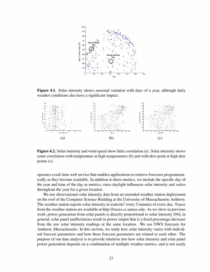
Sunny Winter Day

Cloudy SummerDay

Figure 4.1. Solar intensity shows seasonal variation with days of a year, although dailyweather conditions also have a significant impact.

(a) (b) (c)

Figure 4.2. Solar intensity and wind speed show little correlation (a). Solar intensity showssome correlation with temperature at high temperatures (b) and with dew point at high dewpoints (c).

operates a real-time web service that enables applications to retrieve forecasts programmat-ically as they become available. In addition to these metrics, we include the specific day ofthe year and time of the day as metrics, since daylight influences solar intensity and variesthroughout the year for a given location.

We use observational solar intensity data from an extended weather station deploymenton the roof of the Computer Science Building at the University of Massachusetts Amherst.The weather station reports solar intensity in watts/m2 every 5 minutes of every day. Tracesfrom the weather station are available at http://traces.cs.umass.edu. As we show in previouswork, power generation from solar panels is directly proportional to solar intensity [94]; ingeneral, solar panel inefficiencies result in power output that is a fixed percentage decreasefrom the raw solar intensity readings at the same location. We use NWS forecasts forAmherst, Massachusetts. In this section, we study how solar intensity varies with individ-ual forecast parameters and how these forecast parameters are related to each other. Thepurpose of our data analysis is to provide intuition into how solar intensity and solar panelpower generation depends on a combination of multiple weather metrics, and is not easily

27

(a) (b) (c)

Figure 4.3. Solar intensity generally decreases with increasing values of sky cover (a),relative humidity (b), and precipitation potential (c).

predictable from a single weather metric. The complexity in predicting solar intensity fromone or more weather metrics motivates our study of automatically generating predictionmodels using machine learning techniques in the next section.

Fig. 4.1 shows how the day of the year affects solar intensity by charting the averagesolar intensity reading at noon per day over our 10 month monitoring period, where dayzero is January 1st, 2010. As expected, the graph shows that the solar intensity is lowestin January near the winter solstice and increases into the summer before decreasing afterthe vernal equinox. Additionally, the graph also implies that other conditions also have asignificant impact on solar intensity, since many days throughout the spring and summerhave low solar intensity readings. The graph shows that solar intensity and the day of theyear are roughly correlated: most of the time, but not always, a summer day will have ahigher solar intensity than a winter day. However, other factors must contribute to the solarintensity, since there are clearly some sunny winter days that record higher solar intensityreadings than some cloudy summer days. To better understand correlations with otherweather metrics, we model similar relationships for the other forecast metrics.

For example, Fig. 4.2 shows that wind speed, dew point, and temperature are not highlycorrelated with solar intensity. Solar intensity varies almost uniformly from lower to highervalues at any value of wind speed (a). Thus, wind speed has nearly zero correlation withsolar intensity and its value is not indicative of the solar intensity or solar panel powergeneration. Both temperature (b) and dew point (c) correlate with solar intensity at highervalues: if the temperature or dew point is high, then the solar intensity is likely to behigh. However, if the temperature or dew point is low, the solar intensity exhibits a moresignificant variation between high and low values. The results are intuitive. For example, inthe summer a high temperature is often dependent on sunlight, while in the winter sunlightcontributes less in raising the ambient temperature.

In contrast, Fig. 4.3 shows that sky cover, relative humidity, and chance of precipitationhave high negative correlations with solar intensity. In each case, as the value of the metricincreases, the solar intensity reading generally decreases. However, as with the day of theyear, there must be other factors that contribute to the solar intensity reading, since there aresome days with a high sky cover, relative humidity, and precipitation probability, but a highsolar intensity reading and vice versa. In addition to exhibiting complex relationships withsolar intensity, each weather metric also exhibits a complex relationship with other weather

28

(a) (b) (c)

Figure 4.4. Relative humidity (a) and precipitation % (b) positively correlate with skycover. Relative humidity also increases with increasing precipitation % (c).

Table 4.1. Correlation matrix showing correlation between different forecast parameters.

Day Temp. Dew Wind Sky cover Pcpn. HumidityDay 1.0000 0.7022 0.7007 -0.0711 -0.1034 -0.0571 0.0645Temp. 0.7022 1.0000 0.9212 -0.1994 -0.2582 -0.1279 -0.0791Dew point 0.7007 0.9212 1.0000 -0.2251 0.0455 0.1491 0.3081Wind -0.0711 -0.1994 -0.2251 1.0000 -0.0192 0.0340 -0.1025Sky cover -0.1034 -0.2582 0.0455 -0.0192 1.0000 0.7067 0.7525Precipitation -0.0571 -0.1279 0.1491 0.0340 0.7067 1.0000 0.7475Humidity 0.0645 -0.0791 0.3081 -0.1025 0.7525 0.7475 1.0000

metrics. For example, Fig. 4.4 shows that relative humidity (a) and chance of precipitation(b) exhibit strong, but not perfect correlations, with sky cover, while relative humidity isstrongly correlated with chance of precipitation (c). In all three cases, the metrics rise intandem, although the relationship is noisy due to the value of other weather metrics.

Table 1 shows correlation coefficients for each weather metric using the Pearson product-moment correlation coefficient, which divides the covariance of the two variables by theproduct of their standard deviations. The higher the absolute value of the correlation co-efficient, the stronger the correlation between the two weather metrics—a positive corre-lation indicates an increasing linear relationship, while a negative correlation indicates adecreasing linear relationship. The complex relationships between weather metrics and so-lar intensity shown in this table motivate our study of automated prediction models usingmachine learning techniques in the next section.

4.3 Prediction Models

We represent both observational and forecast weather metrics as a time-series thatchanges due to changing weather patterns and seasons. As the previous section shows,solar intensity depends on multiple weather metrics, which complicates the task of de-veloping an accurate prediction model. The high dimensionality of the time-series datamotivates our study of regression methods to develop solar intensity prediction models.

29

To generate each model we provide eight months of training data (January to August) asinput, which includes solar intensity readings as well as NWS forecasts for 6 weather met-rics. The machine learning techniques automatically output a function that computes solarintensity from the 6 weather metrics, as well as the day of the year. We use the remaining 2months of our data set to test the model’s accuracy. One benefit of using machine learningto automatically generate prediction models is that, in general, the more training data thatis available, the more accurate the model.

We focus our study on short-term forecasts three hours in the future. For our exper-iments, we develop models that determine a relationship at any time t between the solarintensity and the forecast weather metrics three hours in the past (t − 3). Note that we areable to apply our techniques to forecasts of any length; we choose three hours as a simpleillustration. Using our models and the three hour forecast, we are able to compute a pre-diction for the solar intensity three hours in the future. The models we generate are simplefunctions, of the form below, that compute solar intensity from multiple weather metricsincluding the day of the year. We could also add time of the day as an additional metric,but for ease of exposition our experiments focus on predictions at noon. We compare theaccuracy of our models with each other, as well as against a simple model we developed inprior work [94] based solely on the sky condition metric and against a simple past-predicts-future model. Our previous model multiplies the maximum power a solar panel is able togenerate at a given time (of the day and year) by (1-SkyCover), since sky cover representsan estimate of the percentage of the atmosphere the sun is covering.

SolarIntensity = F(Day, Temperature, DewPoint, WindSpeed, SkyCover, Precipitation, Humidity)

F is the function that we determine using different regression methods. We preservethe units of each metric: we represent each day as a value between 0 and 365, temperaturein degrees Fahrenheit, wind speed in miles per hour, sky cover in percentage between 0%and 100%, precipitation potential in percentage between 0% and 100%, and humidity inpercentage between 0% and 100%. However, before applying any regression techniquesbelow we normalize all feature data to have zero mean and unit variance. To quantify theaccuracy of each model, we use the Root Mean Squared Error (RMS-Error) between ourpredicted solar intensity at any time and the actual solar intensity observed. RMS-Error is awell-known statistical measure of the accuracy of values predicted by a time-series modelwith respect to the observed values. An RMS-Error of zero indicates that the model exactlypredicts solar intensity three hours in the future. The closer the RMS-Error is to zero themore accurate the model’s predictions.

4.3.1 Linear Least Squares Regression

We first apply a linear least squares regression method to predict solar intensity. Linearleast squares regression is a simple and commonly-used technique to estimate the relation-ship between a dependent or response variable, e.g., solar intensity, and a set of indepen-dent variables or predictors. The regression minimizes the sum of the squared differencesbetween the observed solar intensity and the solar intensity predicted by a linear approx-imation of the forecast weather metrics. Applying the linear least squares method to the

30

0

200

400

600

800

1000

0 10 20 30 40 50

So

lar

Inte

nsi

ty (

wat

ts/m

^2

)

Days (starting 09/01/2010)

ObservedLinear regression

Figure 4.5. Observed and predicted solar intensity using linear least squares regression forSeptember and October 2010.

eight months of training data yields the prediction model below, with coefficients for eachmetric.

SolarIntensity = 1.18*Day + 77.9*Temp + 33.11*DewPoint + 22.8*WindSpeed - 96.9*SkyCover -49.15*Precipitation - 43.4*Humidity

We verify the prediction accuracy using our test dataset for the remaining months of theyear. We observe the cross validation RMS-Error and prediction RMS-Error in the solarintensity as 165 watts/m2 and 130 watts/m2, respectively. We cross validate the regressionmodel with the training dataset (from Jan. to Aug. 2010) and verify its prediction accuracyusing the testing dataset (Sept. and Oct. 2010). The cross validation RMS-Error quantifieshow well the model predicts values in the training data set, while the prediction RMS-Error predicts how well the model predicts values in the testing data set. Fig. 4.5 showsthe observed and predicted solar intensity for September and October 2010. As the figureshows, the model tracks the solar intensity prediction reasonably accurately, albeit with afew deviations.

4.3.2 Support Vector Machines

We next look at multiple classes of supervised learning methods using Support VectorMachines (SVM) [27]. SVMs, which construct hyperplanes in a multidimensional space,have recently gained popularity for classification and regression analysis. The accuracy ofSVM regression depends on the selection of an appropriate kernel function and parameters.In our work, we studied three distinct SVM kernel functions: a Linear Kernel, a PolynomialKernel, and a Radial Basis Function (RBF) kernel. An SVM uses the kernel function totransform data from the input space to the high-dimensional feature space. We chose SVMsover other supervised learning methods due to its sparsity property and its ability to handlenon-linearity in the data. We use the LibSVM library, which includes a multitude of SVMregression techniques, to implement SVM regression with the linear kernel function onour training data set [28]. We found that both the linear and polynomial kernel performedpoorly with RMS-Errors of 201 watts/m2 and 228 watts/m2, both of which were worse

31

0

200

400

600

800

1000

0 10 20 30 40 50

So

lar

Inte

nsi

ty (

wat

ts/m

2)


ObservedSVM-RBF

Figure 4.6. Observed and predicted solar intensity, using SVM regression with an RBFkernel, for the months of September and October 2010.

0

200

400

600

800

1000

0 10 20 30 40 50

So

lar

Inte

nsi

ty (

wat

ts/m

^2)


ObservedSVM-RBF (4-dimensions)

0

200

400

600

800

1000

0 10 20 30 40 50

So

lar

Inte

nsi

ty (

wat

ts/m

^2)


ObservedCloudy

0

200

400

600

800

1000

0 10 20 30 40 50

So

lar

Inte

nsi

ty (

wat

ts/m

^2)


ObservedPPF

(a) SVM-RBF Kernel (b) Cloudy-FPF (c) PPF

Figure 4.7. Observed and predicted solar intensity, using three different prediction tech-niques — (a) SVM-RBF kernel with 4 dimensions, (b) cloudy computing model using skycondition forecast, (c) past predicts future prediction model — for the months of Septemberand October 2010.

than the linear least squares approach above. As a result, we focus on results using theRBF kernel.

We tested the RBF kernel and SVM using the LibSVM library on our eight months oftraining data. In order to find the optimal parameters for the RBF kernel we ran a grid searchtool from the LibSVM library on the training dataset. We found the optimal parameters ofthe RBF kernel to be cost = 256, γ = 0.015625, and ε = 0.001953125. Using theseparameters, we found that the RBF kernel using all seven dimensions for the seven weathermetrics provides a better regression model than the other regression methods, as indicatedby its low cross validation and prediction errors, both of which are significantly lower thaneither the linear or the polynomial kernels. Fig. 4.6 also reflects this fact in the time-seriesgraph of observed and predicted values. The results show that the RBF kernel also performsbetter than the linear least squares method, having a slightly lower cross validation RMS-error (164 watts/m2) and a slightly higher prediction RMS-Error (163 watts/m2).

32

4.3.3 Eliminating Redundant Information

As we show in the previous section, many weather metrics show a strong correlationwith each other. As a result, our SVM regression models contain redundant information,which often decreases the prediction accuracy of each model. Principal component analy-sis (PCA) is a popular method for removing redundant informations from an input dataset,thereby reducing its dimensionality [29]. Thus, we use the principal component analysisalgorithm to remove redundant informations from our feature dataset. The PCA algorithmuses an orthogonal transformation to convert a set of, potentially correlated, input variablesinto a set of uncorrelated variables called principal components. The number of principalcomponents is less than or equal to the number of original variables. The first principalcomponent has the maximum possible variance, and the second principal component hasthe maximum possible variance under the constraint that it be orthogonal to the first com-ponent, etc.

We choose the first four principal components corresponding to first four (highest)eigenvalues and run the RBF SVM regression method on the reduced feature-set. Theresults (Fig. 4.7(a)) show that the RBF kernel performs better after PCA analysis thanwhen using the full feature-set with a cross validation RMS-Error of 159 watts/m2 and aprediction RMS-error of 128 watts/m2, both of which outperform the linear least squaresmodel. We also ran experiments that further reduced the dimensionality of the feature setfrom 4 to 2. However, we found that all three SVM regression techniques performed worsecompared to the 4-dimentional feature set. The performance degradation is the result of theadditional reduction in dimensionality eliminating information that aids in prediction andis not redundant.

4.3.4 Comparing with Existing Models

Finally, we compare our regression-based prediction models with existing models.First, we compare with a past-predicts-future model (PPF), which uses the previous daysolar intensity to predict the next day solar intensity. Past predicts future models are typ-ically used when forecasts are not available, since the past is a reasonably good indicatorof the future if the weather does not change. While they are highly accurate if weatherconditions do not change, the models are not able to predict drastic changes in the weather.Second, we compare with a simple model that uses only the sky condition as a basis forprediction, called cloudy, which we developed in prior work [94]. We have shown that thecloudy model is more accurate than existing variants of PPF in the literature [30]. Whilethe model is able to predict changes in weather, it does not incorporate information frommultiple weather metrics and their impact on solar intensity.

Fig. 4.7(b) and (c) show how well cloudy and PPF predict weather in our testing dataset, respectively. The results show that while the cloudy model follows the general trend ofthe weather it frequently exhibits wrong predictions. As expected, PPF’s results are inaccu-rate whenever weather changes, which happens nearly every day. By contrast, Fig. 4.7(a)shows that SVM-RBF with the reduced feature provides a much more accurate model. TheRMS-Errors for each model highlight this result: the RMS-Error for SVM-RBF with fourdimensions is 128 watts/m2, while the RMS-Error for cloudy and PPF is 175 and 261, re-

33

spectively. Thus, SVM-RBF with four dimensions is 27% more accurate than the simplecloudy model and 51% more accurate than the PPF model.

4.4 Conclusion

Prior prediction models for solar energy harvesting have been based primarily on theimmediate past [31, 32, 33]. Unfortunately, these methods are unable to predict changes inweather patterns in advance. Since weather forecasts from the NWS are based on aggre-gations of multiple data sources from across the country, they are able to provide advancewarning. The NWS generates forecasts from multiple sophisticated forecast models thatsynthesize a multitude of observational data. We show that the relationship between theseforecast weather metrics and solar intensity is complex. Thus, we automatically deriveprediction models from historical solar intensity and forecast data using machine learningtechniques. We find that models derived using SVMs with RBF kernels and linear leastsquares outperform a past-predicts-future models and a simple model based on sky condi-tion forecasts from prior work [94] and is a promising area for increasing the accuracy ofsolar power generation prediction.

34

CHAPTER 5

MANAGING SERVER CLUSTERS ON INTERMITTENT POWER

The previous two chapters have described weather forecasts based empirical and ma-chine learning models to predict future energy harvesting from renewables. This chapterpresents a new energy abstraction to manage server clusters on renewables or intermit-tent power in general. In this chapter I propose blinking – metered transitions betweena high-power active state and a low-power inactive state – as the primary abstraction forconforming to intermittent power constraints. I design Blink, an application-independenthardware-software platform for developing and evaluating blinking applications, and de-fine multiple types of blinking policies. I then use Blink to design BlinkCache, a blinkingversion of Memcached, to demonstrate the effect of blinking on an example application.


Energy-related costs have become a significant fraction of total cost of ownership (TCO)in modern data centers. Recent estimates attribute 31% of TCO to both purchasing powerand building and maintaining the power distribution and cooling infrastructure [112]. Con-sequently, techniques for reducing the energy footprint of data centers continue to receivesignificant attention in both industry and the research community. We categorize thesetechniques broadly as being either primarily workload-driven or power-driven. Workload-driven systems reconfigure applications as their workload demands vary to use the leastpossible amount of power to satisfy demand. Examples include consolidating load ontoa small number of servers, e.g., using request redirection [49, 41] or VM migration, andpowering down the remaining servers during off-peak hours, or balancing load to mitigatethermal hotspots and reduce cooling costs [37, 60, 61]. In contrast, power-driven systemsreconfigure applications as their power supply varies to achieve the best performance pos-sible given the power constraints.

While prior work has largely emphasized workload-driven systems, power-driven sys-tems are becoming increasingly important. For instance, data centers are beginning to relyon intermittent renewable energy sources, such as solar and wind, to partially power theiroperations [47, 72]. Intermittent power constraints are also common in developing regionsthat experience “brownouts” where the electric grid temporarily reduces its supply underhigh load [41, 75]. Price-driven optimizations, due to either demand-response incentivesor market-based pricing, introduce intermittent constraints as well, e.g., if multiple datacenters coordinate to reduce power at locations with high spot prices and increase powerat locations with low spot prices [66]. Variable pricing is an important tool for demand-side power management of future smart electric grids. The key challenge in power-driven

35

systems is optimizing application performance in the presence of power constraints thatmay vary significantly and frequently over time. Importantly, these power and resourceconsumption constraints are independent of workload demands.

In this chapter, we present Blink, a new energy abstraction for gracefully handling inter-mittent power constraints. Blinking applies a duty cycle to servers that controls the fractionof time they are in the active state, e.g., by activating and deactivating them in succession, togracefully vary their energy footprint. For example, a system that blinks every 30 seconds,i.e., is on for 30 seconds and then off for 30 seconds, consumes half the energy, modulooverheads, of an always-on system. Blinking generalizes the extremes of either keeping aserver active (a 100% duty cycle) or inactive (a 0% duty cycle) by providing a spectrumof intermediate possibilities. Blinking builds on prior work in energy-aware design. First,several studies have shown that turning a server off when not in use is the most effectivemethod for saving energy in server clusters. Second, blinking extends the PowerNap [54]concept, which advocates frequent transitions to a low-power sleep state, as an effectivemeans of reducing idle power waste.

An application’s blinking policy decides when each node is active or inactive at anyinstant based on both its workload characteristics and energy constraints. Clearly, blinkingimpacts application performance, since there may not always be enough energy to powerthe nodes necessary to meet demand. Hence, the goal of a blinking policy is to minimizeperformance degradation as power varies. In general, application modifications are nec-essary to adapt traditional server-based applications for blinking, since these applicationsimplicitly assume always-on, or mostly-on, servers. Blinking forces them to handle regu-lar disconnections more often associated with weakly connected [73] environments, e.g.,mobile, where nodes are unreachable whenever they are off or out of range.

5.1.1 Example: BlinkCache

To demonstrate how blinking impacts a common data center application, we explorethe design of BlinkCache—a blinking version of memcached that gracefully handles in-termittent power constraints—as a proof-of-concept example. Memcached is a distributedmemory cache for storing key-value pairs that many prominent Internet sites, includingLiveJournal, Facebook, Flikr, Twitter, YouTube, and others, use to improve their perfor-mance.

Memcached is a natural first application to optimize for variable power constraints fortwo reasons. First, a memcached cluster is energy-intensive, since it requires continuousoperation of high-memory nodes to ensure instant access to in-memory state. Second,since memcached is performance supplement that is not necessary for correctness, it doesnot preclude a constrained power source that may offer little or no power over some timeperiods. A blinking memcached cluster also exploits the increasing trend toward elevatingmemory in the storage hierarchy, and using it as the primary storage substrate in cloud datacenters [63]. An important consequence of this trend is that applications increasingly usememory less like a cache that only stores a small set of popular objects, and more like astorage system that also stores a long heavy tail of unpopular objects. However, unpopularobjects are not unimportant.

36

0

2

4

6

8

10

1 2000 4000 6000 8000 10000

Milli

ons

of F

ans

Popularity Rank

Facebook

!"#$%&%'()*$&+,"-./$

0")12$.)3($&4$"5')((2$$6'78%&%'()*$&+,"-./$

Figure 5.1. The popularity of web data often exhibits a long heavy tail of equally unpopularobjects. This graph ranks the popularity of Facebook group pages by their number of fans.

For Internet services that store user-generated content, the typical user is often inter-ested in the relatively unpopular objects in the heavy tail, since these objects representeither their personal content or the content of close friends and associates. As one exam-ple, Figure 5.1 depicts a popularity distribution for Facebook group pages in terms of theirnumber of fans. While the figure only shows the popularity rank of the top 10,000 pages,Facebook has over 20 million group pages in total. Most of these pages are nearly equallyunpopular. For these equally unpopular objects, blinking nodes synchronously to handlevariable power constraints results in fairer access to the cache. While fair cache access isimportant, maximizing memcached’s hit rate requires prioritizing access to the most popu-lar objects. We explore these performance tradeoffs in-depth for a memcached cluster withintermittent power constraints.

5.1.2 Contributions

In designing, implementing, and evaluating BlinkCache as a proof-of-concept example,this chapter makes the following contributions.

• Make the Case for Blinking Systems. We propose blinking systems to deal withvariable power constraints in server clusters. We motivate why blinking is a ben-eficial abstraction for dealing with intermittent power constraints, define differenttypes of blinking policies, and discuss its potential impact on a range of distributedapplications.

• Design a Blinking Hardware/Software Platform. We design Blink, an application-independent hardware/software platform to develop and evaluate blinking applica-tions. Our small-scale prototype uses a cluster of 10 low-power motherboards con-nected to a programmable power meter that replays custom power traces and variablepower traces from a solar and wind energy harvesting deployment.

• Design, Implement, and Evaluate BlinkCache. We use Blink to experiment withblinking policies for BlinkCache, a variant of memcached we optimize for intermit-tent power constraints. Our hypothesis is that a load-proportional blinking policy,

37

which keeps nodes active in proportion to the popularity of the data they store, com-bined with object migration to group together objects with similar popularities, re-sults in near optimal cache hit rates, as well as fairness for equally unpopular objects.To validate our hypothesis, we compare the performance of activation, synchronous,and load-proportional policies for realistic Zipf-like popularity distributions. Weshow that a load-proportional policy is significantly more fair than an optimal ac-tivation policy for equally popular objects (4X at low power) while achieving a com-parable hit rate (over 60% at low power).

Section 5.2 provides an overview of blinking systems and potential blinking policies.Section 5.3 presents Blink’s hardware and software architecture in detail, while Section 5.4presents design alternatives for BlinkCache, a blinking version of memcached. Section 5.5then evaluates BlinkCache using our Blink prototype. Finally, Section 5.6 discusses relatedwork and Section 5.7 concludes.

5.2 Blink: Rationale and Overview

Today’s computing systems are not energy-proportional [3]—a key factor that hindersdata centers from effectively varying their power consumption by controlling their uti-lization. Designing energy-proportional systems is challenging, in part, since a varietyof server components, including the CPU, memory, disk, motherboard, and power supply,now consume significant amounts of power. Thus, any power optimization that targets onlya single component is not sufficient, since it reduces only a fraction of the total power con-sumption [3, 51]. As one example, due to the power consumption of non-CPU components,a modern server that uses dynamic voltage and frequency scaling in the CPU at low uti-lization may still operate at over 50% of its peak power [39, 74]. Thus, deactivating entireservers, including most of their components, remains the most effective technique for con-trolling energy consumption in server farms, especially at low power levels that necessitateoperating servers well below 50% peak power on average.

However, data centers must be able to rapidly activate servers whenever workload de-mand increases. PowerNap [54] proposes to eliminate idle power waste and approximatean energy-proportional server by rapidly transitioning the entire server between a high-power active state and a low-power inactive state. PowerNap uses the ACPI S3 state, whichplaces the CPU and peripheral devices in sleep mode but preserves DRAM memory state,to implement inactivity. Transition latencies at millisecond-scale, or even lower, may bepossible between ACPI’s fully active S0 state and its S3 state. By using S3 to emulatethe inactive “off” state. 1 PowerNap is able to consume minimal energy while sleeping.Typical high-end servers draw as much as 40x less power in S3.

Blink extends PowerNap in important ways. First, PowerNap is a workload-driventechnique that eliminates idle server power waste—it uses rapid transitions in a workload-driven fashion to activate each server when work arrives and deactivate it when idle. Incontrast, Blink is a power-driven technique that regulates average node power consumption

1We use “active” and “on” interchangeably to reference ACPI’s S0 state, and inactive and “off” inter-changeably to represent ACPI’s S3 state.

38

Type Model S3 Transition Time (s)Desktop Optiplex 745 13.8Desktop Dimension 4600 12.0Laptop Lenovo X60 11.7Laptop Lenovo T60 9.7Laptop Toshiba M400 9.1Laptop OLPC-XO (w/ NIC) 1.6Laptop OLPC-XO (no NIC) 0.2

Table 5.1. Latencies for several desktop and laptop models to perform a complete S3 cycle(suspend and resume). Data from both [35] and our own measurements of Blink’s OLPC-X0.

independent workload demands. Second, the PowerNap mechanism applies to each serverindependently, while Blink applies to collections of servers. Blinking policies, which weformally define next, are able to capture, and potentially exploit, cross-server dependenciesand correlations in distributed applications. Finally, unlike workload-driven transitions,blinking provides benefits even for the non-ideal S3 transition latencies on the order ofseconds that are common in practice, as we show in Section 5.5.1.3. 2 Table 5.1 showsS3 transition latencies for a variety of platforms, as reported in [35], with the addition ofBlink’s OLPC-X0 nodes. The latencies include both hardware transitions as well as thetime to restart the OS and reset its IP address.

The blink state of each node i is defined by two parameters that determine its dutycycle di, (i) length of the ON interval ton and (ii) length of the OFF interval toff , such thatdi =

tonton+toff

· 100%A blink policy defines the blink state of each node in a cluster, as well as a blink schedule

for each node.The blink schedule defines the clock time at which a specified node transitions its blink

state to active, which in turn dictates the time at which the node turns on and goes off. Theschedule allows nodes to synchronize their blinking with one another, where appropriate.For example, if node A frequently accesses disk files stored on node B, the blink policyshould specify a schedule such that the nodes synchronize their active intervals. To illus-trate how a data center employs blinking to regulate its aggregate energy usage, considera scenario where the energy supply is initially plentiful and there is sufficient workloaddemand for all nodes. In this case, a feasible policy is to keep all nodes continuously on.

Next assume that the power supply drops by 10%, and hence, the data center mustreduce its aggregate energy use by 10%. There are several blink policies that are able tosatisfy this 10% drop. In the simplest case, 10% of the nodes are turned off, while theremaining nodes continue to stay on. Alternatively, another blink policy may specify aduty cycle of di = 90% for every node i. There are also many ways to achieve a per-serverduty cycle of 90% by setting different ton and toff intervals, e.g., ton = 9s and toff = 1sor ton = 900ms and toff = 100ms. Yet another policy may assign different blink states

2PowerNap’s on-demand transitions show little benefit once latencies exceed 100 milliseconds [54].

39

to different nodes, e.g., depending on their loads, such that aggregate usage decreases by10%.

We refer to the first policy in our example above as an activation policy. An activationpolicy only varies the number of active servers at each power level [41, 74] such that someservers are active, while others are inactive; the energy supply dictates the size of the ac-tive server set. In contrast, synchronous policies toggle all nodes between the active andinactive state in tandem. In this case, all servers are active for ton seconds and then inactivefor toff seconds, such that total power usage over each duty cycle matches the availablepower. Of course, since a synchronous policy toggles all servers to active at the same time,it does not reduce peak power, which has a significant impact on the cost of energy pro-duction. An asynchronous policy may randomize the start of each node’s active interval todecrease peak power without changing the average power consumption across all nodes.Finally, an asymmetric policy may blink different nodes at different rates, while ensuringthe necessary change in the energy footprint. For example, an asymmetric policy may beload-proportional and choose per-node blink states that are a function of current load.

All of the policies above are equally effective at capping the average power consump-tion for a variable power signal over any time interval. However, the choice of the blinkpolicy greatly impacts application performance. To see why, consider two common ap-plications: a simple cluster-based web server [41, 49] and an Hadoop cluster [52]. Anactivation policy is well-suited for a cluster-based web server where each node serves staticcontent replicated on each node—by turning off a subset of nodes and evenly redirectingincoming web requests to active servers, the application is able to regulate its energy usageto match its supply. Since any node is able to service any request, transitioning a subset ofthe nodes to the inactive state does not pose a problem. In this case, the application requiresonly minimal changes to accommodate dynamic changes in the set of active servers.

However, an activation policy presents a problem for applications that maintain mem-ory or disk state on specific nodes and exhibit inter-node dependencies. In this case, de-activating nodes will render some application-specific state unavailable. Hadoop is oneexample, since Hadoop’s HDFS file system [68] replicates and stores data chunks of eachfile across many different nodes to improve both performance and data availability. Asa result, simply powering down some nodes for long periods is not effective, since inac-tive nodes may store data necessary for a job to continue execution [52, 38, 48]. One,potentially non-optimal, option for addressing the problem without incurring the overheadof changing the data layout or migrating state prior to deactivating nodes is to leverage asynchronous blinking policy, where all nodes have the same duty cycle. Since all nodesblink between the active and inactive state in tandem, all disk state is accessible duringthe active periods. While the synchronous policy is not necessarily optimal for all appli-cations and maximizes peak power demand, it does eliminate the complexities of dealingwith application-specific communication patterns when determining the blink schedule.However, dealing with application-specific complexities may improve performance: anasynchronous blinking policy may reduce costs by reducing peak power or an asymmetricblinking policy may improve performance by prioritizing nodes that store heavily-accesseddata.

In general, distributed applications that store per-node state require application mod-ifications to gracefully handle blinking, and ensure the state is available at the proper

40

Battery

A

Programmable Power Supply

+ –

Charge Controller

+ –

+ –

+

––

+

V

trace datavia serial port

5M ! 5M !

Experimental Deployment Field Deployment

Power Manager

Low Power Node

Low Power Node

Low Power Node

Low Power Node

Machine Cluster

solar wind

curre

nt d

ata

via

USB

volta

ge d

ata

via

USB

DAQ VoltageLogger

DC CurrentTransducer

Figure 5.2. Hardware architecture of the Blink prototype.

times. However, since intermittent power scenarios may yield little or no power duringcertain periods, it is not appropriate in all application scenarios. For instance, intermit-tent power is not appropriate for applications that make performance guarantees. Theapproach is applicable in many scenarios, such as for best-effort batch jobs, includingHadoop/MapReduce jobs, or for performance optimizations that augment an always-oninfrastructure. In this chapter, we focus on the latter example by developing a version ofmemcached, called BlinkCache, that gracefully handles intermittent power constraints viablinking. While memcached’s design explicitly avoids the type of inter-node dependenciespresent in Hadoop, and other tightly-coupled distributed applications, it is able to benefitfrom an asymmetric load-proportional policy, as we describe in Section 5.4. Additionally,nodes dedicated to memcached deployments do not require disks. Mechanical disks posean additional constraint for blinking due to both performance and reliability concerns withfrequently spinning disks up and down [78]. The effect of power cycling on the lifetimeof CPUs, memory, and motherboards is an open question; we know of no prior work thataddresses the issue.

5.3 Blink Prototype

Blink is a combined hardware/software platform for developing and evaluating blinkingapplications. This section describes our prototype’s hardware and software architecture indetail.

41

5.3.1 Blink Hardware Platform

Blink’s current hardware platform consists of two primary components: (i) a low-powerserver cluster that executes Blink-aware applications and (ii) a variable energy source con-structed using an array of micro wind turbines and solar panels. We use renewable energyto expose the cluster to intermittent power constraints.

5.3.1.1 Energy Sources

We deployed an array of two wind turbines and two solar panels to power Blink. Eachwind turbine is a SunForce Air-X micro-turbine designed for home rooftop deployment,and rated to produce up to 400 watts in steady 28 mph winds. However, in our measure-ments, each turbine generates approximately 40 watts of power on windy days. Our solarenergy source uses Kyocera polycrystalline solar panels that are rated to produce a max-imum of 65 watts at 17.4 volts under full sunlight. Although polycrystalline panels areknown for their efficiency, our measurements show that each panel only generates around30 watts of power in full sunlight and much less in cloudy conditions.

We assume blinking systems use batteries for short-term energy storage and powerbuffering. Modern data centers and racks already include UPS arrays to condition powerand tolerate short-term grid disruptions. We connect both renewable energy sources in ourdeployment to a battery array that includes two rechargeable deep-cycle ResourcePowerMarine batteries with an aggregate capacity of 1320 watt-hours at 12V, which is capableof powering our entire cluster continuously for over 14 hours. However, in this chapter wefocus on energy-neutral operation over short time intervals, and thus use the battery arrayonly as a small 5-minute buffer. We connect the energy sources to the battery pack usinga TriStar T-60 charge controller that provides over-charging circuitry. We deployed ourrenewable energy sources on the roof of a campus building in September 2009 and useda HOBO U30 data logger to gather detailed traces of current and voltage over a period ofseveral months under a variety of different weather conditions.

While our energy harvesting deployment is capable of directly powering Blink’s servercluster, to enable controlled and repeatable experiments we leverage two Extech programmablepower supplies. We use the programmable power supplies, instead of the harvesting de-ployment, to conduct repeatable experiments by replaying harvesting traces, or emulatingother intermittent power constraints, to charge our battery array. 3

Since the battery’s voltage level indicates its current energy capacity, we require sensorsto measure and report it. We use a data acquisition device (DAQ) from National Instrumentsto facilitate voltage measurement. As shown in Figure 5.2, the prototype includes two high-precision 5MOhm resistors between the battery terminals and employs the DAQ to measurevoltage across each resistor. We then use the value to compute the instantaneous batteryvoltage, and hence, capacity. Figure 5.3 shows the empirically-derived capacity of ourprototype’s battery as a function of its voltage level. In addition to battery voltage, weuse DC current transducers to measure the current flowing from the energy source into the

3We are able to set the initial battery level for each experiment using a separate charge controller inload-control mode.

42

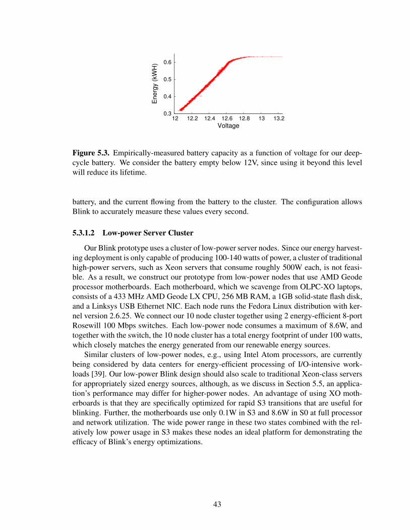
0.3

0.4

0.5

0.6

12 12.2 12.4 12.6 12.8 13 13.2

Ene

rgy

(kW

H)

Voltage

Figure 5.3. Empirically-measured battery capacity as a function of voltage for our deep-cycle battery. We consider the battery empty below 12V, since using it beyond this levelwill reduce its lifetime.

battery, and the current flowing from the battery to the cluster. The configuration allowsBlink to accurately measure these values every second.

5.3.1.2 Low-power Server Cluster

Our Blink prototype uses a cluster of low-power server nodes. Since our energy harvest-ing deployment is only capable of producing 100-140 watts of power, a cluster of traditionalhigh-power servers, such as Xeon servers that consume roughly 500W each, is not feasi-ble. As a result, we construct our prototype from low-power nodes that use AMD Geodeprocessor motherboards. Each motherboard, which we scavenge from OLPC-XO laptops,consists of a 433 MHz AMD Geode LX CPU, 256 MB RAM, a 1GB solid-state flash disk,and a Linksys USB Ethernet NIC. Each node runs the Fedora Linux distribution with ker-nel version 2.6.25. We connect our 10 node cluster together using 2 energy-efficient 8-portRosewill 100 Mbps switches. Each low-power node consumes a maximum of 8.6W, andtogether with the switch, the 10 node cluster has a total energy footprint of under 100 watts,which closely matches the energy generated from our renewable energy sources.

Similar clusters of low-power nodes, e.g., using Intel Atom processors, are currentlybeing considered by data centers for energy-efficient processing of I/O-intensive work-loads [39]. Our low-power Blink design should also scale to traditional Xeon-class serversfor appropriately sized energy sources, although, as we discuss in Section 5.5, an applica-tion’s performance may differ for higher-power nodes. An advantage of using XO moth-erboards is that they are specifically optimized for rapid S3 transitions that are useful forblinking. Further, the motherboards use only 0.1W in S3 and 8.6W in S0 at full processorand network utilization. The wide power range in these two states combined with the rel-atively low power usage in S3 makes these nodes an ideal platform for demonstrating theefficacy of Blink’s energy optimizations.

43

Blinking InterfacesetDutyCycle(int nodeId, int onPercentage)setBlinkInterval(int nodeId, int interval)syncActiveTime(int node, long currentTime)forceSleep(int nodeId, int duration)

Table 5.2. Blink APIs for setting per-node blinking schedules.

Measurement InterfacegetBatteryCapacity()getBatteryEnergy()getChargeRate(int lastInterval)getDischargeRate(int lastInterval)getServerLoadStats(int nodeId)

Table 5.3. Blink’s measurement APIs that applications use to inform their blinking deci-sions.

5.3.2 Blink Software Architecture

Blink’s software architecture consists of an application-independent control plane thatcombines a power management service with per-node access to energy and node-levelstatistics. Blink-aware applications interact with the control plane using Blink APIs toregulate their power consumption. The power management service consists of a powermanager daemon that runs on a gateway node and a power client daemon that runs oneach cluster node. The architecture separates mechanism from policy by exposing a singlesimple interface for applications to control blinking for each cluster node.

The power manager daemon has access to the hardware sensors, described above, thatmonitor the battery voltage and current flow. Each Blink power client also monitors host-level metrics on each cluster node and reports them to the power manager. These metricsinclude CPU utilization, network bandwidth, and the length of the current active period.The power client exposes an internal RPC interface to the power manager that allows it toset a node’s blinking pattern. To set the blinking pattern, the power client uses the timer ofthe node’s real-time clock (RTC) to automatically sleep and wake up, i.e., transition backto S0, at specific intervals. Thus, the power client is able to set repetitive active and inactivedurations. For example, the power manager may set a node to repeatedly be active for 50seconds and inactive for 10 seconds. In this case, the blink interval is 60 seconds with thenode being active 83% of the time and inactive 17% of the time. We assume that nodessynchronize clocks using a protocol such as NTP to enable policies that coordinate blinkschedules across cluster nodes.

The impact of clock synchronization is negligible for our blink intervals at the gran-ularity of seconds, but may become an issue for blink intervals at the granularity of mil-liseconds or less. Note that clock synchronization is not an issue for applications, such

44

as memcached, that do not perform inter-node communication. Transitioning between S0and S3 incurs a latency that limits the length of the blink interval. Shorter blink inter-vals are preferable since they allow each node to more closely match the available power,more rapidly respond to changes in supply, and reduces the battery capacity necessaryfor short term buffering. The XO motherboard yields S3 sleep latencies that range fromroughly 200 milliseconds to 2 seconds depending on the set of active devices and drivers(see Table 5.1). For instance, since our USB NIC driver does not implement the ACPIreset resume function, we must unload and load its driver when transitioning to andfrom S3. As a result, the latency for our experiments is near 2 seconds. Unfortunately,inefficient and incorrect device drivers are commonplace, and represent one of the currentdrawbacks to blinking in practice.

The Blink control plane exposes an RPC interface to integrate with external applicationsas shown in Tables 5.2 and 5.3. Applications use these APIs to monitor input/output currentflow, battery voltage, host-level metrics and control per-node blinking patterns. Since Blinkis application-independent, the prototype does not report application-level metrics. In suchcases, an application must monitor itself. For instance, for some policies in our blinkingversion of memcached, a proxy monitors per-key hit rates, as described in Section 5.4.3.1.

5.4 Blinking Memcached

Memcached is a distributed in-memory cache for storing key-value pairs that signifi-cantly reduces both the latency to access data objects and the load on persistent disk-backedstorage. Memcached has become a core component in Internet services that store vastamounts of user-generated content, with services maintaining dedicated clusters with 100sto 1000s of nodes [63]. Since end users interact with these services in real-time throughweb portals, low-latency access to data is critical. High page load latencies frustrate usersand may cause them to stop generating new content [62], which is undesirable since theseservices’ primary source of revenue derives from their content, e.g., by selling targeted ads.

5.4.1 Memcached Overview

Memcached’s design uses a simple and scalable client-server architecture, where clientsrequest a key value directly from a single candidate memcached server with the potentialto store it. Clients use a built-in mapping function to determine the IP address of thiscandidate server. Initial versions of memcached determined the server using the functionHash(Key)%NumServers, while the latest versions use the same consistent hashingapproach popularized in DHTs, such as Chord [71]. In either case, the key values randomlymap to nodes without regard to their temporal locality, i.e., popularity. Since all clients usethe same mapping function, they need not communicate with other clients or servers tocompute which server to check for a given key. Likewise, Memcached servers respond toclient requests (gets and sets) without communicating with other clients or servers. Thislack of inter-node communication enables Memcached to scale to large clusters.

Importantly, clients maintain the state of the cache, including its consistency with per-sistent storage. As a result, applications are explicitly written to use memcached by (i)

45

100101102103104105106107

100 101 102 103 104 105 106 107 108

Num

ber o

f Fan

s

Popularity Rank

FacebookZipf

Figure 5.4. The popularity rank, by number of fans, for all 20 million public group pageson Facebook follows a Zipf-like distribution with α = 0.6.

checking whether an object is resident in the cache before issuing any subsequent queries,(ii) inserting a newly referenced object into the cache if it is not already resident, and (iii)updating a cached object to reflect a corresponding update in persistent storage. Each mem-cached server uses the Least Recently Used (LRU) replacement policy to evict objects. Onecommon example of a cached object is an HTML fragment generated from the results ofmultiple queries to a relational database and other services. Since a single HTTP requestfor many Internet services can result in over 100 internal, and potentially sequential, re-quests to other services [63, 43], the cache significantly decreases the latency to generatethe HTML.

5.4.2 Access Patterns and Performance Metrics

The popularity of web sites has long been known to follow a Zipf-like distribution [40,76], where the fraction of all requests for the i-th most popular document is proportional to1/iα for some constant α. Previous studies [40, 76] have shown that α is typically less thanone for web site popularity. The key characteristic of a Zipf-like distribution is its heavytail, where a significant fraction of requests are for relatively unpopular objects. We expectthe popularity of user-generated content for an Internet service to be similar to the broaderweb, since, while some content may be highly popular, such as a celebrity’s Facebookpage, most users are primarily interested in either their own content or the content of closefriends and associates.

As a test of our expectation, we rank all 20 million user-generated fan pages on Face-book by their number of fans. We use the size of each page’s fan base as a rough ap-proximation of the popularity of its underlying data objects. Figure 5.4 confirms that thedistribution is Zipf-like with α approximately 0.6. Recent work also states that Facebookmust store a significant fraction of their data set in massive memcached cluster, i.e., on theorder of 2000 nodes, to achieve high hit rates, e.g., 25% of the entire data set to achievea 96.5% hit rate [63]. This characteristic is common for Zipf-like distributions with lowα values, since many requests for unpopular objects are inside the heavy tail. Thus, thedistribution roughly divides objects into two categories: the few highly popular objects and

46

the many relatively unpopular objects. As cache size increases, it stores a significant frac-tion of objects that are unpopular compared to the few popular objects, but nearly uniformlypopular compared to each other. These mega-caches resemble a separate high-performancestorage tier [63] for all data objects, rather than a small cache for only the most popular dataobjects.

Before discussing different designs alternatives for BlinkCache, we define our perfor-mance metrics. The primary cache performance metric is hit ratio, or hit rate, which repre-sents the percentage of object requests that the cache services. A higher hit rate indicatesboth a lower average latency per request, as well as lower load on the back-end storagesystem. In addition to hit rate, we argue that fairness should be a secondary performancemetric for large memcached clusters that store many objects of equal popularity. A faircache distributes its benefits—low average request latency—equally across objects. Cachesare usually unfair, since their primary purpose is to achieve high hit rates by storing morepopular data at the expense of less popular data. However, fairness increases in impor-tance when there are many objects with a similar level of popularity, as in today’s largememcached clusters storing data that follows a Zipf-like popularity distribution. An unfaircache results in a wide disparity in the average access latency for these similarly popularobjects, which ultimately translates to end-users receiving vastly different levels of perfor-mance. We use the standard deviation of average request latency per object as our measureof fairness. The lower the standard deviation the more fair the policy, since this indicatesthat objects have average latencies that are closer to the mean.

5.4.3 BlinkCache Design Alternatives

We compare variants of three basic memcached policies for variable power constraints:an activation policy, a synchronous policy, and an asymmetric load-proportional policy.In all cases, any get request to an inactive server always registers as a cache miss, whileany set request is deferred until the node becomes active. We defer a discussion of theimplementation details using Blink to the next section.

• Activation Policy. An activation policy ranks servers 1...N and always keeps thetop M servers active, where M is the maximum number of active servers the currentpower level supports. We discuss multiple activation variants, including a static vari-ant that does not change the set of available servers in each client’s built-in mappingfunction to reflect the current set of active servers, and a dynamic variant that doeschange the set. We also discuss a key migration variant that continuously ranks thepopularity of objects and migrates them to servers 1...N in rank order.

• Synchronous Policy. A synchronous policy keeps all servers active for time t andinactive for time T − t for every interval T , where t is the maximum duration thecurrent power level supports and T is short enough to respond to power changesbut long enough to mitigate blink overhead. The policy does not change the set ofavailable servers in each client’s built-in mapping function, since all servers are activeevery interval.

47

• Load-Proportional Policy. A load-proportional policy monitors the aggregate pop-ularity of objects Pi that each server i stores and keeps each server active for timeti and inactive for time T − ti for every interval T . The policy computes each ti bydistributing the available power in the same proportion as the aggregate popularity Piof the servers. The load-proportional policy also migrates similarly popular objectsto the same server.

5.4.3.1 Activation Policy

A straightforward approach to scaling memcached as power varies is to activate serverswhen power is plentiful and deactivate servers when power is scarce. One simple methodfor choosing which servers to activate is to rank them 1...N and activate and deactivatethem in order. Since, by default, memcached maps key values randomly to servers, ourpolicy for ranking servers and keys is random. In this case, a static policy variant that doesnot change each client’s built-in mapping function to reflect the active server set arbitrar-ily favors keys that happen to map to higher ranked servers, regardless of their popularity.As a result, requests for objects that map to the top-ranked server will see a significantlylower average latency than requests for objects that happen to map to the bottom-rankedserver. One way to correct the problem is to dynamically change the built-in client mappingfunction to only reflect the current set of active servers. With constant power, dynamicallychanging the mapping function will result in a higher hit rate since the most popular objectsnaturally shift to the current set of active servers.

Hash-based Key Mapping. Memcached recently added support for consistent hashing toreduce the disruption from changing a cluster’s size. The original function (Hash(Key)%NumServers)invalidates nearly every key when adding or removing a single server from a cluster of sizen. Only the keys that have both the old NumServers and the new NumServers ascommon factors do not change mappings. The approach is clearly not scalable, since eachchange, regardless of size, flushes nearly the entire cache, which abruptly increases load onthe back-end storage system, as well as request latency, until the cache re-populates itself.

Consistent hashing, originally popularized [71] by DHTs, significantly improves thesituation, since adding or removing each server only invalidates 1/nth of the keys for acluster of size n. The approach scales gracefully, since the percentage of keys the cacheinvalidates by changing a single server in the active set decreases as cluster size increases.However, consistent hashing is not a panacea when power varies either frequently or signif-icantly. For instance, if the available power doubles, thereby doubling the number of activeservers, a consistent hashing approach will still invalidate 50% of its resident objects. Witha dynamic approach, frequent variations in power repeatedly incur this steep invalidationpenalty.

Thus, while our dynamic variant results in a higher hit rate than a static variant underconstant power, the opposite is true, due to invalidation penalties, for power that variesfrequently or significantly. One option for eliminating invalidation penalties entirely is toexplicitly control the mapping of individual keys to servers, and pro-actively migrate themost popular objects to the most popular servers. Figure 5.5 illustrates a memcached designthat interposes an always-active proxy between memcached clients and servers to control

48

PHP Server

MCD Client

Application Server

PHP Server

MCD Client

Application Server

MCD Proxy

Power Manager

Power ClientMCD Server

Backend (OLPC)

Power ClientMCD Server

Backend (OLPC)

Frontend (SheevaPlug)

Battery

Figure 5.5. To explicitly control the mapping of keys to servers, we interpose always-activerequest proxies between memcached clients and servers. The proxies are able to monitorper-key hit rates and migrate similarly popular objects to the same nodes.

the mapping. In this design, clients issue requests to the proxy, which maintains a hashtable that stores the current mapping of keys to servers, issues requests to the appropriateback-end server, and returns the result to the client.

Table-based Key Mapping. Since all requests pass through the proxy, it is able to continu-ously monitor and sort the popularity of objects in the background and dynamically changethe server mappings as popularities change. Note that to migrate an object the proxy needonly change its key→server mapping. After the change, the next key request for the ob-ject will incur one cache miss on the new server, which results in application-level codere-generating and re-inserting the object at the new location. The proxy may either pro-actively evict the object from the old server or simply allow LRU replacement to evict theobject. This strategy eliminates invalidation penalties, since popularity-based migrationalways places the most popular objects on the highest-ranked servers. The design requiresno changes to either memcached clients or servers.

Deactivating lower-ranked servers invalidates objects that are already less popular thanobjects on the higher-ranked active servers, while activating additional servers grows thesize of the cache without invalidating the more popular objects that are already resident.The approach does introduce the overhead of monitoring and sorting keys by popularity,as well as proxying requests through an intermediary server. However, these overheadcosts are independent of power variations and amortized over time, rather than imposedabruptly at each change in the power level. The proxy approach scales to multiple proxiesby allowing memcached clients to use their original built-in mapping function to map keysto a set of proxies instead of a set of servers, such that each proxy is responsible for arandom subset of keys.

In a multi-proxy design, the proxies periodically send popularity statistics to a centralserver that sorts them in the background and distributes each proxy a new server mapping.The period between re-mappings is a function of both how fast key popularity is changingand the number of keys in the cache, since drastic popularity changes require re-mappingsand more keys increase the time to gather, sort, and distribute new mappings. Changes toserver mappings need not be highly synchronized across all proxies, though, since mem-

49

cached provides no guarantees that data is present or consistent with a back-end database.A multi-proxy design allows the proxies to share the bandwidth and processing load ofissuing client requests to servers, while maintaining the ability to explicitly control keymappings.

We expect a few-to-many relationship between proxies and memcached servers, al-though highly-loaded memcached clusters may require a mapping as low as one-to-one.In this case, the argument for using proxies instead of the nodes themselves mirrors Som-niloquy’s argument for using low-power, augmented network interfaces to perform simpleapplication functions on behalf of sleeping nodes [35]. Another consideration for a proxy-based migration approach is the load imposed on the highest-ranked memcached servers. Ifthe highest-ranked servers become overloaded, the re-mapping process may need to placea few less popular keys on high-ranked nodes to ensure they are not overloaded. Thetechnique is analogous to Popularity-based Data Concentration (PDC) for disk arrays thatmust be careful not to deactivate too many disks and then overload the remaining activedisks [65].

5.4.3.2 Synchronous Policy

The migration-enabled activation policy, described above, approaches the optimal pol-icy for maximizing the cache’s hit rate, since ranking servers and mapping objects to themaccording to popularity rank makes the distributed cache operate like a centralized cachethat simply stores the most popular objects regardless of the cache’s size. We define opti-mal as the hit rate for a centralized cache of the same size as the distributed Memcachedinstance under the same workload. However, the policy is unfair for servers that store simi-larly popular objects, since these servers should have equal rankings. The activation policyis forced to arbitrarily choose a subset of these equally ranked servers to deactivate. In thiscase, a synchronous policy is significantly more fair and results in nearly the same hit rateas the optimal activation policy. To see why, consider the simple 4-node memcached clus-ter in Figure 5.6 with enough available power to currently activate half the cluster. Thereis enough power to support either (i) our activation policy with migration that keeps twonodes continuously active or (ii) a synchronous policy that keeps four nodes active half thetime but synchronously blinks them between the active and inactive state.

For now we assume that all objects are equally popular, and compare the expected hitrate and standard deviation of average latency across objects for both policies, assuming afull cache can store all objects at full power on the 4 nodes. For the activation policy, thehit rate is 50%, since it keeps two servers active and these servers store 50% of the objects.Since all objects are equally popular, migration does not significantly change the results. Inthis case, the standard deviation is 47.5ms, assuming an estimate of 5ms to access the cacheand 100ms to regenerate the object from persistent storage. For a synchronous policy, thehit rate is also 50%, since all 4 nodes are active half the time and these nodes store 100%of the objects. However, the synchronous policy has a standard deviation of 0ms, since allobjects have a 50% hit probability, if the access occurs when a node is active, and a 50%miss probability, if the access occurs when a node is inactive. Rather than half the objectshaving a 5ms average latency and half having a 100ms average latency, as with activation,a synchronous policy ensures an average latency of 52.5ms across all objects.

50

Keyset A

Keyset B

Keyset C

Keyset D

Keyset A

Keyset B

Keyset C

Keyset D

Keyset A

Keyset C

Keyset B

Keyset D

(a)

(b)

(c)

Power

Power

100% On

Power

100% On

Power

100% On

Power

100% OnKeyset

CMigrated

Keyset D

Migrated

0% On

Power

0% On

Power

0% On

Power

0% On

Power Power

50% On

Power Power

50% On 50% On 50% On

Figure 5.6. Graphical depiction of a static/dynamic activation blinking policy (a), an acti-vation blinking policy with key migration (b), and a synchronous blinking policy (c).

Note that the synchronous policy is ideal for a normal memcached cluster with a map-ping function that randomly maps keys to servers, since the aggregate popularity of objectson each server will always be roughly equal. Further, unlike an activation policy that usesthe dynamic mapping function, the synchronous policy does not incur invalidation penaltiesand is not arbitrarily unfair to keys on lower-ranked servers.

5.4.3.3 Load-Proportional Policy

A synchronous policy has the same hit rate as an activation policy when keys have thesame popularity, but is significantly more fair. However, an activation policy with migrationis capable of a significantly higher hit rate for highly skewed popularity distributions. Aproportional policy combines the advantages of both approaches for Zipf-like distributions,where a few key values are highly popular but there is a heavy, but significant, tail ofsimilarly unpopular key values. As with our activation policy, a proportional policy ranksservers and uses a proxy to monitor object popularity and migrate objects to servers in rankorder. However, the policy distributes the available power to servers in the same proportionas the aggregate popularity of their keys.

For example, assume that in our 4 server cluster after key migration the percentageof total hits that go to the first server is 70%, the second server is 12%, the third serveris 10%, and the fourth server is 8%. If there is currently 100W of available power thenthe first server ideally receives 70W, the second server 12W, the third server 10W, andthe fourth server 8W. These power levels then translate directly to active durations overeach interval T . In practice, if the first server’s maximum power is 50W, then it will beactive the entire interval, since its maximum power is 70W. The extra 20W is distributedto the remaining servers proportionally. If all servers have a maximum power of 50W, thefirst server receives 50W, the second server receives 20W, i.e., 40% of the remaining 50W,the third server receives 16.7W, and the fourth server receives 13.3W. These power levelstranslate into the following active durations for a 60 second blink interval: 60 seconds, 24seconds, 20 seconds, and 16 seconds, respectively.

51

Metric Workload Best PolicyHit Rate Uniform SynchronousHit Rate Zipf Activation (Migration)Fairness Uniform/Zipf Synchronous

Fairness + Hit Rate Zipf Load-Proportional

Table 5.4. Summary of the best policy for a given performance metric and workload com-bination.

The hit rate from a proportional policy is only slightly worse than the hit rate from theoptimal activation policy. In this example, we expect the hit rate from an activation policyto be 85% of the maximum hit rate from a fully powered cluster, while we expect the hit ratefrom a proportional policy to be 80.2%. However, the policy is more fair to the 3 servers—12%, 10%, and 8%—with similar popularities, since each server receives a similar totalactive duration. The Zipf distribution for a large memcached cluster has similar attributes.A few servers store highly popular objects and will be active nearly 100% of the time, whilea large majority of the servers will store equally unpopular objects and blink in proportionto their overall unpopularity.

5.4.4 Summary

Table 5.4 provides a summary of the best policy for each performance metric and work-load combination. In essence, an activation policy with key migration will always have thehighest hit rate. However, for distributions with equally popular objects, the synchronouspolicy achieves a similar hit rate and is more fair. A load-proportional policy combines thebest attributes of both for Zipf-like distributions, which include a few popular objects butmany similarly unpopular objects.

5.5 Implementation and Evaluation

We implement and evaluate the BlinkCache design alternatives from the previous sec-tion using our small-scale Blink prototype. The purpose of our evaluation is not to maxi-mize the performance of our particular memcached deployment or improve on the perfor-mance of the custom memcached server deployments common in industry. Instead, ourgoal is to explore the effects of churn on memcached caused by power fluctuations fordifferent BlinkCache designs. Our results will differ across platforms according to the spe-cific blink interval, CPU speed, and network latency and bandwidth of the servers and thenetwork. Since our prototype uses low-power CPUs and motherboards, the request laten-cies we observe in our prototype are not representative of those found in high performanceservers.

Each node in Blink connects to a low-power (2.4W/switch) 100 Mbps switch and runsan instance of Blink’s power client and an unmodified memcached server. We wrote amemcached client workload generator to issue key requests at a configurable, but steady,

52

rate according to either a Zipf popularity distribution, parameterized by α, or a uniformpopularity distribution. As in a typical application, the workload generator fetches anydata not resident in the cache from a MySQL database and places it in the cache. Sincewe assume the MySQL server provides always-available persistent storage, it runs off thepower grid and not variable power. Note that for our benchmarks we take the conservativeapproach of simply fetching key values directly from MySQL with a single query, and donot imitate the sequential, multi-query nature of production web applications. While we donot model or evaluate the impact of workloads that include multi-get memcached requeststhat issue gets for multiple keys in parallel, blinking with key migration should not impactthe performance of multi-get requests for keys with similar popularities, e.g., part of thesame HTML page, since our proxy will migrate these keys to the same server.

Unless otherwise noted, in our experiments, we use moderate-size objects of 10 kilo-bytes, Facebook-like Zipf α values of 0.6, and memcached’s consistent hashing mappingfunction. Each experiment represents a half-hour trace, we configure each memcachedserver with a 100MB cache to provide an aggregate cache size of 1GB, and we use ourprogrammable power supply to drive each power trace. Since each node has only 256MBof memory, we scale our workloads appropriately for evaluation. We modify magent, apublicly available memcached proxy, 4 to implement the design alternatives in the previ-ous section, including table-based key mapping and popularity-based key migration. Ourmodifications are not complex: we added or changed only 300 lines of code to implementall of the BlinkCache design variants from Section 5.3. Since all requests pass through theproxy, it is able to monitor key popularity. The proxy controls blinking by interacting withBlink’s power manager, which in our setup runs on the same node, to monitor the availablepower and battery level and set per-node blinking patterns. We also use the proxy for ex-periments with memcached’s default hash-based key mappings, rather than modifying thememcached client. Since our always-on proxy is also subject to intermittent power con-straints, we run it on a low-power (5W) embedded SheevaPlug with a 1.2 GHz ARM CPUand 512 MB of memory.

We first use our workload generator to benchmark the performance of each blinkingpolicy for both Zipf-like and uniform popularity distributions at multiple power levels withvarying levels of oscillation. We then demonstrate the performance for an example webapplication—tag clouds in GlassFish—using realistic traces from our energy harvestingdeployment that have varying power and oscillation levels.

5.5.1 Benchmarks

We measure the maximum power of each node, at 100% CPU and network utilization,in S0 to be 8.6W and its minimum power in S3 to be 0.2W. We use these values in theproxy to compute the length of active and inactive periods to cap power consumption at aspecific level. We also measure the impact of our node’s near 2 second transition latencyfor blink intervals T between 10 seconds and 2 minutes. Figure 5.7 shows the results fora duty cycle of 50%. In this case, the blinking interval must be over 40 seconds beforeaverage power over the interval falls below 55% of the node’s maximum power, as we

4http://code.google.com/p/memagent/

53

0

20

40

60

80

100

0 10 20 40 60 80 100 120

% o

f Ful

l Pow

er

Blink Interval (50 % Duty Cycle)

Figure 5.7. The near 2 second latency to transition into and out of S3 in our prototypediscourages blinking intervals shorter than roughly 40 seconds. With a 50% duty cycle weexpect to operate at 50% full power, but with a blink interval of less than 10 seconds weoperate near 100% full power.

0

30

60

90

120

1 10 100

Thr

ough

put (

Mbp

s)

Value Size (KB)

DedicatedProxy

MySQL

0

50

100

150

200

250

1 10 100

Late

ncy

(mse

c)

Value Size (KB)

DedicatedProxy

MySQL (get)

(a) Throughput (b) Latency

Figure 5.8. Maximum throughput (a) and latency (b) for a dedicated memcached server,our memcached proxy, and a MySQL server. Our proxy imposes only a modest overheadcompared with a dedicated memcached server.

expect. The result shows that on-demand transitions that occur whenever work arrives ordeparts are not practical in our prototype. Further, even blinking intervals as high as 10seconds impose significant power inefficiencies. As a result, we use a blinking interval of60 seconds for our experiments. Our 60 second blink interval is due solely to limitations inthe Blink prototype. Note that there is an opportunity to significantly reduce blink intervalsthrough both hardware and software optimizations. Since server clusters do not typicallyleverage ACPI’s S3 state, there has been little incentive to optimize its transition latency.

Next, we determine a baseline workload intensity for memcached, since, for certainrequest rates and key sizes, the proxy or the switch becomes a bottleneck. In our experi-ments, we use a steady request rate (1000 get requests/sec) that is less than the maximumrequest rate possible once the proxy or switch becomes a bottleneck. Note that our re-sults, which focus on hit rates, are a function of the popularity of objects rather than thedistribution of request inter-arrival times. Our goal is to evaluate how blinking affects the

54

0

20

40

60

80

100

120

80% 45% 20%

Hit

Rat

e (%

)

% of Full Power

Activation (Static)Activation (Dynamic)

Activation (Key Migration)

Figure 5.9. Under constant power for a Zipf popularity distribution, the dynamic variant ofthe activation policy performs better than the static variant as power decreases. However,the activation policy with key migration outperforms the other variants.

relative hit rates between the policies, and not the performance limitations of our particu-lar set of low-power components. Figure 5.8 demonstrates the maximum performance, interms of total throughput and request latency for different key values sizes, of an unmod-ified memcached server, our memcached proxy, and a MySQL server. As expected, thememcached server provides an order of magnitude higher throughput and lower request la-tency than MySQL. Further, our proxy implementation imposes only a modest overhead toboth throughput and latency, although the latency impact of proxy-based redirections willbe greater on faster CPUs since less relative request time is spent in the OS and network.Our subsequent experiments focus on request hit rates rather than request latencies, sincelatencies vary significantly across platforms and workloads. Further, the wide disparity inlatency between serving a request from memory and serving it from disk would show alarger, and potentially unfair, advantage for a blinking system. Thus, we consider hit rate abetter metric than latency for evaluating a blinking memcached instance.

5.5.1.1 Activation Blinking and Thrashing

An activation policy for an unmodified version of memcached must choose whether ornot to alter the hash-based mapping function as it activates and deactivates servers. Forconstant power, a dynamic mapping function that always reflects the currently active setof servers should provides the best hit rate, regardless of the popularity distribution, sinceapplications will be able to insert the most popular keys on one of the active servers. Fig-ure 5.9 demonstrates this point for a workload with a Zipf popularity distribution (α = 0.6),and shows the hit rates for both static and dynamic activation variants at multiple constantpower levels. While at high power levels the approaches have similar hit rates, as powerlevel decreases, we see that the static variant incurs a higher penalty under constant power.However, Figure 5.10 demonstrates that the opposite is true for highly variable power. Thefigure reports hit rates for different levels of power oscillation, where the average powerfor each experiment is 45% of the power necessary to run all nodes concurrently. The x-axis indicates oscillation level as a percentage, such that 0% oscillation holds power steady

55

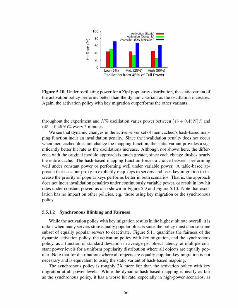
0

20

40

60

80

100

Low (5%) Mid. (25%) High (50%)

Hit

Rat

e (%

)

Oscillation from 45% of Full Power

Activation (Static)Activation (Dynamic)


Figure 5.10. Under oscillating power for a Zipf popularity distribution, the static variant ofthe activation policy performs better than the dynamic variant as the oscillation increases.Again, the activation policy with key migration outperforms the other variants.

throughout the experiment and N% oscillation varies power between (45 + 0.45N)% and(45− 0.45N)% every 5 minutes.

We see that dynamic changes in the active server set of memcached’s hash-based map-ping function incur an invalidation penalty. Since the invalidation penalty does not occurwhen memcached does not change the mapping function, the static variant provides a sig-nificantly better hit rate as the oscillations increase. Although not shown here, the differ-ence with the original modulo approach is much greater, since each change flushes nearlythe entire cache. The hash-based mapping function forces a choice between performingwell under constant power or performing well under variable power. A table-based ap-proach that uses our proxy to explicitly map keys to servers and uses key migration to in-crease the priority of popular keys performs better in both scenarios. That is, the approachdoes not incur invalidation penalties under continuously variable power, or result in low hitrates under constant power, as also shown in Figure 5.9 and Figure 5.10. Note that oscil-lation has no impact on other policies, e.g. those using key migration or the synchronouspolicy.

5.5.1.2 Synchronous Blinking and Fairness

While the activation policy with key migration results in the highest hit rate overall, it isunfair when many servers store equally popular objects since the policy must choose somesubset of equally popular servers to deactivate. Figure 5.11 quantifies the fairness of thedynamic activation policy, the activation policy with key migration, and the synchronouspolicy, as a function of standard deviation in average per-object latency, at multiple con-stant power levels for a uniform popularity distribution where all objects are equally pop-ular. Note that for distributions where all objects are equally popular, key migration is notnecessary and is equivalent to using the static variant of hash-based mapping.

The synchronous policy is roughly 2X more fair than the activation policy with keymigration at all power levels. While the dynamic hash-based mapping is nearly as fairas the synchronous policy, it has a worse hit rate, especially in high-power scenarios, as

56

0

10

20

30

40

50

80% 45% 20%

Sta

ndar

d D

evia

tion

% of Full Power

SynchronousActivation (Key Migration)

Activation (Dynamic)

Figure 5.11. For a uniform popularity distribution, both the synchronous policy and thedynamic variant of the activation policy are significantly more fair, i.e., lower standarddeviation of average per-object latency, than the activation policy with key migration.

0

20

40

60

80

100

120

80% 45% 20%

Hit

Rat

e (%

)

% of Full Power

SynchronousActivation (Key Migration)

Activation (Dynamic)

Figure 5.12. For a uniform popularity distribution, the synchronous policy and the activa-tion policy with key migration achieve a similar hit rate under different power levels. Bothpolicies achieve a better hit rate than the dynamic variant of the activation policy.

shown in Figure 5.12. Thus, the synchronous policy, which is more fair and provides loweraverage latency, is a better choice than any variant of the activation policy for uniformpopularity distributions. Note that the key popularity distribution across servers in everymemcached cluster that uses a hash-based mapping function is uniform, since keys mapto servers randomly. Thus, the synchronous policy is the best choice for a heavily-loadedmemcached cluster that cannot tolerate the throughput penalty of using proxies.

5.5.1.3 Balancing Performance and Fairness

Activation with key migration results in the maximum hit rate for skewed popular-ity distributions where some objects are significantly more popular than others, while thesynchronous policy results in the best overall performance, in terms of both hit rate andfairness, for uniform popularity distributions. The proportional policy combines the advan-

57

0

10

20

30

40

50

80% 45% 20%

Sta

ndar

d D

evia

tion

% of Full Power

Load ProportionalActivation (Key Migration)

Synchronous

Figure 5.13. The load-proportional policy is more fair to the unpopular objects, i.e. bot-tom 80% in popularity, than the activation policy with key migration for Zip popularitydistributions, especially in low-power scenarios.

0

20

40

60

80

100

120

80% 45% 20%

Hit

Rat

e (%

)

% of Full Power

Load ProportionalActivation (Key Migration)

Synchronous

Figure 5.14. The load-proportional policy has a slightly lower hit rate than the activationpolicy with key migration.

tages of both and works well for Zipf-like distributions with a few popular objects but along tail of similarly (un)popular objects, since the long heavy tail in isolation is similar tothe uniform distribution. Figure 5.14 shows the hit rate for the proportional policy, the acti-vation policy with migration, and the synchronous policy for a Zipf popularity distributionwith α = 0.6 at different power levels. The synchronous policy performs poorly, especiallyat low power levels, in this experiment, since it does not treat popular objects different thanunpopular objects.

However, the proportional policy attains nearly the same hit rate as the activation pol-icy at high power levels, since it also prioritizes popular objects over unpopular objects.Even at low power levels its hit rate is over 60% of the activation policy’s hit rate. Fur-ther, the proportional policy is significantly more fair to the many unpopular objects in thedistribution. Figure 5.13 reports fairness, in terms of the standard deviation in per-objectlatency, at different power levels for the unpopular keys, i.e., keys ranked in the bottom80th percentile of the distribution. The activation policy’s unfairness is nearly 4X worse at

58

0

20

40

60

80

100

0 1 2 3 4 5 6 7 8 9 10

Hit

Rat

e (%

)

S3 Transition Overhead (sec)

Load ProportionalSynchronous


Figure 5.15. As S3 transition overhead increases, the hit rate from the load-proportionalpolicy decreases relative to the activation policy with key migration for a Zipf distributionat a moderate power level.

0

20

40

60

80

100

120

0 30 60 90 120 150 180

Pow

er (

wat

ts)

Time (minutes)

Power Supply

0

100

200

300

400

500

0 30 60 90 120 150 180

Load

Lat

ency

(m

sec)

Time (minutes)

Load ProportionalSynchronous


(a) Power (b) Page Load Latency

Figure 5.16. Power signal from a combined wind/solar deployment (a) and average pageload latency for that power signal (b).

low power levels. Thus, the proportional policy strikes a balance between performance andfairness when compared against both the synchronous and activation policies.

Finally, Figure 5.15 shows how the S3 transition overhead affects our results at a mod-erate power level. The figure shows that the overhead has only a modest effect on theload-proportional policy’s hit rate. The overhead does not affect the relative fairness ofthe policies. Note that all of our previous experiments use our prototype’s 2 second transi-tion overhead. A shorter transition overhead would improve our results, and even a longertransition would show some, albeit lesser, benefits.

5.5.2 Case Study: Tag Clouds in GlassFish

While our prior experiments compare our blinking policies for different power andoscillation levels, we also conduct an application case study using traces from our energyharvesting deployment. The experiment provides a glimpse of the performance tradeoffsfor realistic power signals. GlassFish is an open source Java application server from Sun,

59

which includes a simple example application that reuses parts of the Java PetStore multi-tier web application, used in prior research, e.g., [42], to create tag clouds for pets. Tagclouds are a set of weighted tags that visually represent the most popular words on a webpage. We modify the default web application to generate HTML for per-user tag cloudpages and cache them in memcached. The data to construct each HTML page comes froma series of 20 sequential requests to a MySQL database.

For these experiments, we measure the latency to load user tag cloud pages, whichincorporates MySQL and HTML regeneration latencies whenever HTML pages are notresident in the cache. The MySQL latency for our simple table-based data is typically 30msper database query. While page load latency follows the same trend as hit rate, it providesa better application-level view of the impact of different policies. Figure 5.16(b) shows theaverage latency to load user web pages across 40,000 users for our three different policies—activation with key migration, proportional, and synchronous—for a combined solar andwind trace, assuming the popularity of each user’s tag cloud page follows a Zipf distributionwith α = 0.6. We derive the power signal, shown in Figure 5.16(a), by compressing a 3-dayenergy harvesting trace to 3 hours.

As expected, the activation policy with key migration and the load-proportional policyexhibit comparable page load latencies at most points in the trace. For this trace, the load-proportional policy is within 15% of the activation policy’s hit rate. The activation policyis slightly better at low energy levels, since it tends to strictly ensure that more popularcontent is always cached. Also as expected, the synchronous policy tends to perform poorlyacross all power levels. Also as expected, we measure the standard deviation of page loadlatencies for the load-proportional policy to be within 2% to the synchronous policy for thevast majority, i.e., bottom 80%, of the equally unpopular objects.

5.6 Related Work

The sensor network community has studied strategies for dealing with variable sourcesof renewable power, since these systems often do not have access to the power grid. How-ever, since sensor networks are geographically distributed, each node must harvest its ownenergy, resulting in network-wide energy imbalances [44], whereas data center nodes sharea common power delivery infrastructure. Further, the primary performance metric for asensor network is the amount of data the network collects. As a result, much of the energyharvesting work is not directly applicable to data centers. Similarly, mobile computinggenerally focuses on extending battery life by regulating power consumption [77], ratherthan modulating performance to match energy production.

The increasing energy consumption of data centers [34] has led companies to investheavily in renewable energy sources [59, 72]. For example, the goal of Google’s RE<Cinitiative is to make large-scale renewable power generation cheaper than coal-based pro-duction. As a result, researchers have started to study how to incorporate renewables into adata center’s power delivery infrastructure [70]. As one example, Lee et al. [50] use requestredirection to control the carbon footprint of data centers by redirecting load to serverspowered by renewable energy sources. While not directly related to energy harvesting,Power Routing [64] proposes shuffled power delivery topologies that allow data centers

60

to control how much power each rack receives. While the topologies are well-suited fordelivering variable amounts of power to racks based on aggregate demand, they are alsouseful for flexible routing of a variable power supply. Prior research on workload-drivenapproaches to improve data center energy efficiency is orthogonal to our work. Examplesinclude designing platforms that balance CPU and I/O capacity [39, 69], routing requests tolocations with the cheapest energy [66], and dynamically activating and deactivating nodesas demand rises and falls [41, 74, 49]. PowerNap’s node-level energy proportional tech-nique has also been viewed as a workload-driven optimization [54]. We show that a similartechnique is useful for controlling per-node power consumption in a power-driven system.

Power capping has also been studied previously in data centers to ensure collections ofnodes do not exceed a worst-case power budget [67, 45]. However, the work assumes ex-ceeding the power budget is a rare transient event that does not warrant application-specificmodifications, and that traditional power management techniques, e.g., DVFS, are capableof enforcing the budget. These assumptions may not hold in many scenarios with inter-mittent power constraints, as with our renewable energy power source. Gandhi et al. capCPU power by forcing CPU idle periods [46]. While similar, blinking focuses on cappingper-node power where the CPU is only one component of the total power draw. Improvingthe energy-efficiency of storage is also a related research area. While Memcached doesnot offer persistent storage, our modifications for blinking adapt similar ideas from priorstorage research, such as migrating popular objects to more active nodes [65, 78]. Addi-tionally, power-aware caching algorithms focus on maximizing the idle time between diskaccesses to reduce disk power consumption, while our work focus on controlling the powerconsumption of the cache itself [82].

Blinking introduces regulated churn into data center applications as nodes switch fromthe active to inactive state. Churn has been well-studied in decentralized, self-organizingdistributed hash tables [71]. However, the type of churn experienced by DHTs is differentthan the churn caused by blinking, which motivates our different approach to the problem.In the former case, nodes arrive and depart unexpectedly based on autonomous user be-havior and network conditions, while in the latter case, nodes switch between the activeand inactive states in a regular and controllable fashion. Finally, RAMCloud [63] proposesusing memory for low-latency persistent storage, and cites as motivation the increasinglylarge memcached clusters used in production data centers. The size of these clusters mo-tivates our observation that fairness for the large number of equally unpopular objects, inaddition to hit rate, is an important performance metric.

5.7 Conclusion

In this chapter, we focus on managing server clusters running on intermittent power. Wepropose blinking as the primary abstraction for handling intermittent power constraints, anddefine multiple types of blinking policies. We then design an application-independent plat-form for developing and evaluating blinking applications, and use it to perform an in-depthstudy of the effects of blinking on one particular application and power source: mem-cached operating off renewable energy. We find that while an activation policy with keymigration results in the best hit rates, it does not distribute the benefits of the cache equally

61

among equally popular objects. As in-memory caches continue grow in size, they willstore a greater fraction of equally popular objects for Zipf-like object popularity distribu-tions. We then propose and evaluate an asymmetric load-proportional policy to increasefairness without significantly sacrificing the cache’s hit rate.

62

CHAPTER 6

DISTRIBUTED FILE SYSTEM FOR INTERMITTENT POWER

As discussed in the previous chapter, designing systems to operate under intermittentpower is challenging, since applications often access persistent distributed state, wherepower fluctuations can impact data availability and I/O performance. To support concurrentstateful applications on a blinking cluster, in this chapter, I design a blink-aware distributedfile system, which combines blinking with a power-balanced data layout and popularity-based replication/reclamation to optimize I/O throughput and latency as power varies.


The growth of cloud-based services continues to fuel a rapid expansion in the size andnumber of data centers. The trend only exacerbates the environmental and cost concernsassociated with data center power usage, which a recent report estimates at 1.7-2.2% ofU.S. consumption [124]. Excessive energy consumption also has serious environmentalramifications, since 83% of U.S. electricity derives from burning “dirty” fossil fuels [125].Energy costs are also on a long-term upward trend, due to a combination of governmentregulations to limit carbon emissions, a continuing rise in global energy demand, and dwin-dling supplies. Even with today’s “cheap” power, a data center’s energy-related costs rep-resent a significant fraction (∼31% [112]) of its total cost of ownership. Prior research ongreen data centers often assumes that grid energy is always available in unlimited quanti-ties [110, 111], and focuses largely on optimizing applications to use less energy withoutimpacting performance. By comparison, there has been little research on optimizing appli-cations for intermittent power that fluctuates over time. Operating off intermittent powerintroduces new opportunities for optimizing a data center to be both cheaper and greener.

The ability to use intermittent power introduces other opportunities, beyond increasinguse of renewable energy, for optimizing a data center to be cheaper, greener, and morereliable. We argue that designing systems to exploit these optimizations will move uscloser to the vision of a net-zero data center.

• Market-based Electricity Pricing. Electricity prices vary continuously based onsupply and demand. Many utilities now offer customers access to market-based ratesthat vary every five minutes to an hour [107]. As a result, the power data centersare able to purchase for a fixed price varies considerably and frequently over time.For instance, in the New England hourly wholesale market in 2011, maintaining afixed $55/hour budget, rather than a fixed per-hour power consumption, purchases16% more power for the same price (Figure 6.1). The example demonstrates that

63

0

1

2

3

4

0 60 120 180 240 300

Pow

er (

MW

)

Days

$55/hour Budget

Figure 6.1. Electricity prices vary every five minutes to an hour in wholesale markets,resulting in the power available for a fixed monetary budget varying considerably overtime.

data centers that execute delay-tolerant workloads, such as data-intensive batch jobs,have an opportunity to reduce their electric bill by varying their power usage basedon price.

• Unexpected Blackouts or Brownouts. Data centers often use UPSs for backuppower during unexpected blackouts. An extended blackout may force a data cen-ter to limit power consumption at a low level to extend UPS lifetime. While lowpower levels impact performance, it may be critical for certain applications to main-tain some, even low, level of availability, e.g., disaster response applications. As wediscuss, maintaining availability at low power levels is challenging if applicationsaccess distributed state. Further, in many developing countries, the electric grid ishighly unstable with voltage rising and falling unexpectedly based on changing de-mands. These “brownouts” may also affect the power available to data centers overtime.

• 100% Power Infrastructure Utilization. Another compelling use of intermittentpower is continuously operating a data center’s power delivery infrastructure at 100%.Since data center capital costs are enormous, maximizing the power delivery infras-tructure’s utilization by operating as many servers as possible is important. However,data centers typically provision power for peak demands, resulting in low utiliza-tion [114, 123]. In this case, intermittent power is useful to continuously run a back-ground workload on a set of servers—designed explicitly for intermittent power—that always consume the excess power PDUs are capable of delivering. Since the uti-lization (and power usage) of a data center’s foreground workload may vary rapidly,the background servers must be capable of quickly varying power usage to not exceedthe power delivery infrastructure’s limits.

In this chapter, we present the design of a distributed file system (DFS) for intermit-tent power. Since DFSs now serve as the foundation for a wide range of data-intensiveapplications run in today’s data centers, taking advantage of any of the opportunities abovenecessitates a DFS optimized for intermittent power. As we discuss, designing such a DFS

64

poses a significant research challenge, since periods of scarce power may render data in-accessible, while periods of plentiful power may require costly data layout adjustments toscale up I/O throughput.

Our work is the first to address the problem by designing a blink-aware stateful DFSoptimized for intermittent power. Our system, called BlinkFS, represents a dramatic de-parture from all prior techniques used in energy-efficient storage systems, which generallyrely on powering down large sets of servers for long periods of time to reduce overall en-ergy consumption. Our goal is to design a DFS that performs well across a wide range ofintermittent power scenarios – ranging from large and rapid power variations (+/- 90%) tosustained low power periods (∼20%). In all cases, BlinkFS’s goal is to utilize intermittentpower as efficiently as possible, rather than guarantee a specific amount of work finisheswithin some time period. Since intermittent power may not be available to satisfy work-loads with strict performance requirements or deadlines, it is not appropriate in these cases.Since we focus on using intermittent power, optimizations that use grid energy in combi-nation with renewables to provide SLA guarantees are beyond the scope of this thesis. Aswe describe in Section 6.2, the dynamics of intermittent power, where changes in availablepower may be significant, frequent, and unpredictable, warrant our new approach. Below,we highlight the advantages of our DFS designed for intermittent power, called BlinkFS,over co-opting prior energy-efficient storage techniques, e.g., [38, 48, 126, 65, 129, 78].

• Low Amortized Overhead. Blinking every node at regular intervals prevents costlyand abrupt data migrations—common in many systems—whenever power decreases—to concentrate data on a small set of active nodes—or increases—to spread data outand increase I/O throughput. Instead, blinking ensures that each node is active, andits data is accessible, for some period of time each blink interval, at the expense of amodest overhead to transition each node between a high-power active and low-powerinactive state.

• Bounded Replica Inconsistency. Deactivating nodes for long periods requires writeoff-loading to temporarily cache writes destined for inactive or overloaded nodes [117].The technique requires excessive writes whenever nodes activate or deactivate to ei-ther apply or migrate off-loaded writes, respectively, while impacting reliability ifoff-loaded writes are lost due to a node failure. In contrast, BlinkFS ensures allreplicas are consistent within one blink interval of any write, regardless of the powerlevel.

• No Capacity Limitations. Since migrating to a new data layout is expensive, agoal of BlinkFS is to decouple I/O performance at any power level from the datalayout: the same layout should perform well at all power levels. To ensure sucha data layout, Rabbit [38] severely limits the capacity of nodes storing secondary,tertiary, etc. replicas. Blinking enables a power-independent layout without suchlimitations.

• Minimally Disruptive. DFSs support higher-level applications designed assumingfully active nodes with stable data layouts. Frequently changing the set of active

65

nodes or the data layout disrupts scheduling and placement algorithms for applica-tions, such as MapReduce, that co-locate computation with DFS storage. BlinkFSis less disruptive, since it keeps every node active for the same duration every blinkinterval and does not change the data layout as power varies.

• Always-accessible Data. Prior systems render data completely inaccessible if thereis not enough power to store all data on the set of active nodes. In contrast, BlinkFSensures all data is accessible, with latency bounded by the blink interval, even at lowpower levels where the set of active nodes is unable to store the entire data set.

Since each node’s data is inaccessible for some period each blink interval, BlinkFS’sgoal is to gain the advantages above without significantly degrading access latency. Inachieving this goal, this chapter makes the following contributions.Blinking-aware File System Design. We detail BlinkFS’s design and its advantages overco-opting existing energy-proportional DFSs for intermittent power. The design leveragesa few always-active proxies to absorb file system operations, e.g., reads and writes, whilemasking BlinkFS’s complexity from applications.Latency Reduction Techniques. We discuss techniques for mitigating blinking’s latencypenalty. Our approach combines staggered node active intervals with a power-balanceddata layout to ensure replicas stored on different nodes are active for the maximum durationeach blink interval. BlinkFS also uses popularity-based data replication and reclamation tofurther decrease latency for frequently-accessed data blocks.Implementation and Evaluation. We implement BlinkFS on a small-scale prototype us-ing 10 Mac minis connected to a programmable power supply that drives variable powertraces. We then benchmark BlinkFS’s performance and overheads at different (fixed andoscillating) power levels. We also compare BlinkFS with prior energy-efficient DFSs intwo intermittent power scenarios—maintaining a fixed-budget despite variable prices andusing intermittent wind/solar energy— using three different applications: a MapReduce-style batch system, the MemcacheDB key-value store, and file system traces from a searchengine. As an example of our results, BlinkFS improves MapReduce job completion timeby 42% at 50% power compared to an existing energy-proportional DFS. At 20% power,BlinkFS still finishes jobs, while existing approaches stall completely due to inaccessibledata.

6.2 DFSs and Intermittent Power

Reducing data center power consumption is an active research area. Much prior workfocuses on energy-proportional systems, where power usage scales linearly with workloaddemands [3]. The goal of energy-proportional systems is to not impact performance: ifdemands increase, these systems increase power consumption to maintain performance.Energy-proportional distributed applications typically vary power consumption by activat-ing and deactivating nodes as workload demands change. An obvious approach for ad-dressing intermittent power is to co-opt existing energy-proportional approaches, but varythe number of active nodes in response to changes in available power rather than workloaddemands. Unfortunately, as we discuss below, the approach does not work well for DFSs

66

using intermittent power, since power variations may be significant, frequent, and unpre-dictable, e.g., from changing prices, explicit demand response signal sent by the electricgrid, or wind, solar, geothermal, etc. power. While energy-proportional systems optimizeenergy consumption to satisfy workload demands, designing for intermittent power re-quires systems to optimize performance as power varies. Below, we summarize how inter-mittent power affects energy-proportional DFSs, and then discuss two specific approaches.

6.2.1 Energy-Proportional DFSs

DFSs, such as the Google File System (GFS) [122] or the Hadoop Distributed FileSystem (HDFS) [68], distribute file system data across multiple nodes. Designing energy-proportional DFSs is challenging, in part, since naıvely deactivating nodes to reduce energyusage has the potential to render data inaccessible [126]. One simple way to prevent dataon inactive nodes from becoming inaccessible is by storing replicas on active nodes. Repli-cation is already used to increase read throughput and reliability in DFSs, and is effectiveif the fraction of inactive nodes is small. For example, with HDFS’s random placementpolicy for replicas, the probability that any block is inaccessible is m!(n−k)!

n!(m−k)! for n nodes, minactive nodes, and k replicas per block. Figure 6.2 plots the fraction of inaccessible dataas a function of the fraction of inactive nodes, and shows that nearly all data is accessi-ble for small numbers of inactive nodes. However, the fraction of inaccessible data risesdramatically once half the nodes are inactive, even for aggressive replication factors, suchas k=7. Further, even a few inactive nodes, where the expected percentage of inaccessibledata is small, may pose problems, e.g., by stalling batch jobs dependent on a small portionof the inaccessible data.

Thus, a popular approach for designing energy-efficient storage systems is to use con-centrated data layouts, which deactivate nodes without causing inaccessible data. Thelayouts often store primary replicas on one subset of nodes, secondary replicas on anothermutually-exclusive subset, tertiary replicas on another subset, etc., to safely deactivate non-primary nodes [38, 126]. Other systems concentrate data to optimize for skewed access pat-terns, by storing only popular data on a small subset of active nodes [116, 121, 48, 65, 78].Unfortunately, concentrated layouts cause problems if available power varies indepen-dently of workload demands. Below, we highlight three problems with approaches thatuse concentrated data layout to deactivate nodes for long periods.Inaccessible Data. If there is not enough power available to activate the nodes necessaryto store all data, then some data will become inaccessible at low power levels. As wemention in Section 6.1, sustained low power periods are common in many intermittentpower scenarios, such as during extended blackout or brownout periods, when using on-site solar generation on a cloudy day, or maintaining a fixed power budget as energy pricesrise. Thus, gracefully degrading throughput and latency down to extremely low powerlevels is important. With concentrated data layouts, as data size increases, the number ofnodes, and hence minimum power level, required to store all data and keep it accessibleincreases.Write Off-loading Overhead. Energy-proportional systems leverage write off-loading totemporarily cache writes on currently active nodes, since clients cannot apply writes toinactive nodes, e.g., [117, 38, 129]. Write off-loading is also useful for deferring writes

67

0

20

40

60

80

100

0 20 40 60 80 100

Inaccessib

le D

ata

(%

)

Inactive Nodes (%)

k=1k=3k=7

Figure 6.2. Inaccessible data rises with the fraction of inactive nodes using a randomreplica placement policy.

to overloaded nodes, which are common when only a small number of active nodes storeall data. While a small number of active primary nodes decreases the minimum powerlevel necessary to keep data accessible, it overloads primaries by requiring them to processall writes. The approach also imposes abrupt overheads when activating or deactivatingnodes, either to apply off-loaded writes to newly active nodes or overloaded primary nodes,respectively. Further, intermittent sources, e.g., wind power, that exhibit abrupt powervariations require near immediate node deactivations, precluding the completion of time-consuming operations. While using a large battery array as a buffer mitigates the impact ofsudden variations, it is prohibitively expensive [119]. Further, deferring writes to replicason inactive nodes degrades reliability in the event of node failure. Failure’s consequencesare worse during low power periods, by increasing the number of off-loaded writes onactive nodes, and the time replicas on inactive nodes remain in an inconsistent state.Disrupts Higher-level Application. A common paradigm for DFSs in data centers is todistribute file system data across compute nodes that host a variety of distributed appli-cations. These applications, e.g., MapReduce, have their own, often highly optimized,algorithms to schedule and place computation to minimize data transfer overheads. Thus,activating and deactivating nodes or changing data layouts as power varies often requiressignificant modifications to higher-level applications.

Below, we outline two approaches to energy-proportional DFSs that use concentrateddata layouts and vary power by activating and deactivating nodes. We highlight the addi-tional problems these DFSs encounter if power variations are significant and frequent.

6.2.2 Migration-based Approach

We classify any approach that varies power consumption by migrating data to concen-trate it on a set of active nodes, and then deactivating the remaining nodes, as a migration-based approach. With this approach, power variations trigger changes to number of nodesstoring either the most popular data or primary, secondary, tertiary, etc. replicas. In ei-ther case, data layout changes require migrations to spread data out to provide higher I/Othroughput (as nodes become active) or to concentrate data and keep it accessible (as nodesbecome inactive). Thus, mitigating migration overheads is a focus of prior work on energy-efficient storage [48, 65, 78].

68

D1

D1

D1

Time

100%

50%

25%

D2

D2

D2

D3

D3

D3

D4

D4

D4

D1 D2

D2D4

D3 D4

D1D3

D2D4

D1D3

(b)(a)

Figure 6.3. Simple example using a migration-based approach (a) and blinking (b) to dealwith power variations.

To highlight the problems with this approach, consider the simple example in Fig-ure 6.3(a), where there is enough power to operate four nodes storing primary replicasand the data fills two nodes’ storage capacity. A sudden and unexpected drop in power by2X, leaving only two active nodes, may not afford enough time for the necessary migra-tions, leaving some data inaccessible. Even with sufficient time for migration, an additional2X power drop, leaving only one active node, forces at least 50% of the data to becomeinaccessible. Note that we focus on regulating power consumption within a single datacenter. Another way to handle power variations is to migrate applications and their datato remote data centers with ample or cheap power [118]. The technique is infeasible forlarge storage systems. Even assuming dedicated high-bandwidth network links, we viewfrequent transfers of large, e.g., multi-petabyte, storage volumes as impractical.

6.2.3 Equal-Work Approach

Amur et al. propose an energy-proportional DFS, called Rabbit, that eliminates migration-related thrashing using an equal-work data layout [38]. The layout uses progressively largerreplica sets, e.g., more nodes store (n + 1)-ary replicas than n-ary replicas. Specifically,the layout orders nodes 1 . . . i and stores bi = B

iblocks on the ith node, where i > p and

p nodes store primary replicas (assuming a data size of B). The layout ensures that any1 . . . k active nodes (for k < i total nodes) are capable of servicing B

kblocks, since B

i< B

k.

Since the approach is able to spread load equally across any subset of nodes in the idealcase of reading all data, it ensures energy-proportionality with no migrations.

Amur et al. provide details of the approach in prior work [38], including its performancefor workloads that diverge from the ideal. Rabbit’s primary constraint is its storage capacitylimitations as i → ∞, since B

idefines the capacity for node i. Thus, for N homogeneous

nodes capable of each storing M blocks, the nodes’ aggregate storage capacity is MN ,while Rabbit’s storage capacity is pM +

∑Ni=p+1

pMi

= O(logN). For example, for N=500nodes and M=214=16384 64MB blocks, the aggregate storage capacity across all nodes

69

is MN=500 terabytes, while Rabbit’s capacity is less than 15 terabytes, or 3% of totalcapacity, when p=2.

The relationships above show that the fraction of unused capacity increases linearlywith N . Thus, the total storage capacity is capable of accommodating significantly morereplicas than Rabbit uses as N increases. To reduce capacity limitations, Rabbit is able toindividually apply the layout to multiple distinct data sets, by using a different 1 . . . i nodeordering for each data set. However, multiplexing the approach between data sets tradesoff desirable energy-efficient properties, e.g., few nodes storing primary replicas and idealenergy-proportionality. Thus, Rabbit’s design presents issues for large clusters of nodeswith similar storage capacities.

6.3 Applying Blinking to DFSs

The systems in the previous section use activation policies that vary power consump-tion only by varying the number of active nodes. As discussed in Chapter 5, the blinkingabstraction supports many other types of blinking policies. As we discuss in Section 6.4,BlinkFS uses an asynchronous staggered blinking policy.

To see the advantages of blinking for DFSs, recall the previous section’s example (Fig-ure 6.3(b)), where there is initially enough power to operate four nodes that each providestorage for a fraction of the data. If the available power decreases by 2X, with blinking wehave the option of keeping all four nodes active for time tactive = t

2every blink interval t.

In this case, instead of migrating data and concentrating it on two active nodes, we are ableto keep the same data layout as before without changing our aggregate I/O throughput overeach blink interval, assuming each node has the same I/O throughput when active. Thus,at any fixed power level, blinking is able to provide the same I/O throughput, assumingnegligible transition overheads, as an activation approach. However, blinking has a distinctadvantage over a migration-based approach if the available power changes, since it is pos-sible to alter node active intervals nearly instantly to match the available power without theoverhead of migration. Additionally, in contrast to Rabbit, the blinking approach does notrequire severe capacity limitations on nodes to maintain throughput. Finally, the approachis beneficial at low power levels if not enough nodes are active to store all data, since datais accessible for some period each blink interval.

6.4 BlinkFS Design

Figure 6.4 depicts BlinkFS’s architecture, which resembles other recent DFSs, includ-ing GFS [122], HDFS [68], Rabbit [38], etc., that use a master meta-data server to coordi-nate access to each node’s data via a block server. The master also maintains the file systemnamespace, tree-based directory structure, file name→ blocks mapping, and block→ nodemapping, as well as enforces the access control and block placement and replication policy.As in prior systems, files consist of multiple fixed-size blocks replicated on zero or morenodes. To mitigate the impact of node failure, the master may recover from meta-data in-formation stored at one or more proxies, described below, or maintain an up-to-date copyof its meta-data on backup nodes.

70

File Metadata Server---------------------- Power

Manager

Power ClientBlock Server



Application BlinkFS Client

Power Signal

data

BlinkFSLegend:

Data msg.Control msg.

FUSE

blk 1blk 2

blk k

bs 1bs 2

bs n

/bob/test

create, ls / get BS states

write <filename, offset, data>

read 

<blink states, CPU utils, I/O rates>

<Blin

k stat

e (sta

rt tim

e, on

perio

d)>

<CPU util, I/O rate>

Blinking Nodesmetadata

info.

File Proxy<blink states, CPU utils, I/O

rates>

get block metadata



write (repli

cate)



FS metadata / BS states

cp 

Figure 6.4. BlinkFS Architecture

BlinkFS also includes a power manager that monitors available power, as well as anyenergy stored in batteries, using hardware sensors. The power manager implements a blink-ing policy that continuously alters per-node blinking patterns to match power consumptionwith available power. Specifically, the power manager communicates with a power clienton each node to set the blink interval duration t, as well as its start time and active interval(tactive). The power client also acts as an interface for accessing other resource utilizationstatistics, including CPU utilization, I/O accesses, etc. The power manager informs themaster and proxies, described below, of the current blinking policy, i.e., when and howlong each node is active every blink interval, and per-node resource utilization statistics.To access the file system, higher-level applications interact with BlinkFS clients throughwell-known file system APIs. Our prototype uses the POSIX API’s file system calls.

We do not assume that BlinkFS clients are always active, since clients may run onblinking nodes themselves, e.g., in clusters that co-locate computation and DFS storage.Thus, to enable clients to read or write blocks on inactive nodes, BlinkFS utilizes one ormore always-active proxies to intercept read and write requests if a client and block serverare not concurrently active, and issue them to the appropriate node when it next becomesactive. Each proxy maintains a copy (loaded on startup by querying the master) of the meta-data information necessary to access a specific group of files (each file is handled by a singleproxy), and ensures replica consistency every blink interval. The proxy propagates any filesystem operations that change meta-data information to the master before committing thechanges. The power manager also maintains an up-to-date view of each node’s power state,since each power client sends it a status message when transitioning to or from the inactivestate. The messages also serve as heartbeats: if the power manager does not receive anystatus messages from a power client within some interval, e.g., 5 minutes, it checks if itsblock server has failed. A failure prompts the master to initiate recovery actions.

Similar to a set of always-active nodes storing primary replicas, proxies consume powerthat increases the minimum threshold required to operate the cluster. Importantly, however,proxies only serve as intermediaries, and do not store data. As a result, the data set size doesnot dictate the number of proxies. However, proxies do limit I/O throughput by redirecting

71

(1)

(2)

Blink Interval

(3)

(4)

Nodes

R1

Staggered

(5)

(6)

(7)

(8)

R2

R3

R4(if necessary)

R1

R3

R2

Node 1

Node 2

Node 3

Node 4

Node 5

Node 6

Node 7

Node 8

1st

2nd

3rd4th (if necessary)

(a) Staggered Blinking (b) Power-balanced Data Layout

Figure 6.5. Combining staggered blinking (a) with a power-balanced data layout (b) max-imizes block availability.

communication between many clients and block servers through a few points. However, aswe discuss below, mostly-active clients may often bypass the proxies when accessing data.Further, proxies are most useful at low power levels, where available power, rather thanproxy performance, limits I/O throughput. Below we discuss the details of how BlinkFS’scomponents facilitate reading and writing files, and then present techniques for mitigatingBlinkFS’s high latency penalty.

6.4.1 Reading and Writing Files

Proxies mask the complexity of interacting with blinking nodes from applications. Themaster and each client use a well-known hash function to map a file’s absolute path to aspecific proxy. To read or write a file, clients either issue requests to the proxy directly, oruse an optimization, discussed below, that bypasses a file’s proxy if the client is active atthe same time as the file’s block servers.Handling Reads. The meta-data necessary to read a file includes its block IDs and theirversion numbers, as well as the (IP) address and blinking information of the block serversstoring replicas of the file’s blocks. The proxy holds read requests until a node storing theblock becomes active, issues the request to the block server, receives the data, and thenproxies it to the client. If multiple block servers storing the block’s replicas are active, theproxy issues the request to the node with the longest remaining active interval, assumingthe remaining active time exceeds a minimum threshold necessary to read and transmit theblock. Using a proxy to transfer data is necessary when executing both clients and blockservers on blinking nodes, since the client may not be active at the same time as the blockserver storing the requested data.

To optimize reads, mostly-active clients may directly request from the proxy the blockinformation—IDs and version numbers—and blinking policy for each block server holdinga replica, and then access block servers directly when they become active. The optimizationsignificantly reduces the proxy load for read-intensive workloads. To ensure the proxyapplies all previous client writes to a block before any subsequent reads, the proxy includes

72

a version number for each block, incremented on every update, in its response to the client.If the version number for the block stored at the block server is lower than the requestedversion number, then the proxy holds pending writes that it has not yet applied. In this case,the read stalls until the proxy applies the writes and the version numbers match. If the blockserver has an equivalent or higher version number, it sends back the data immediately. Ineither case, a block server ensures that a client never gets stale data, i.e., a block of versionnumber lower than the requested version number. Like a Unix file system, application-levelfile locking might be necessary to ensure the atomicity of cross-block reads, e.g., as in thecase of concurrent producers and consumers.Handling Writes. The proxy performs a similar sequence for writes. All writes flowthrough a file’s proxy, which serializes concurrent writes and ensures all block replicas areconsistent each blink interval. The proxy may also return to the client before applyingthe write to every block replica, since subsequent reads either flow through the proxy ormatch version numbers at the block server, as described above. The proxy maintains anin-memory write-ahead log to track pending off-loaded writes from clients. Since the logis small, the proxy stores in-memory backups on one or more nodes (updated on each writebefore returning to the client), which it recovers from after a failure. When the client issuesthe write, the proxy first records the request in its log, increments the version number ofthe updated blocks, updates the master metadata and its own metadata, and returns to theclient; next it then propagates the write to all replicas as the block servers become active;finally, when all replicas successfully apply the write, it removes the request from its log ofpending writes.

Since all block servers are active for a period each blink interval, all replicas are consis-tent within one blink interval from when the write is issued, and the maximum time a writeremains pending in the proxy’s log is one blink interval. Of course, the proxy does have afixed-size log for pending writes. After filling the log, further write requests stall until theproxy propagates at least one of its queued writes to each replica. Based on available powerand the CPU and network utilization of block servers, the proxy limits write throughput toensure all pending writes are applied within a blink interval, e.g., by stalling additionalwrites.

As with reads, mostly-active clients could also interact directly with block servers, aslong as the client and block server are both active at the same time. In this case, the proxymaintains an intermediate version number for each block, not visible to read requests, tohandle concurrent writes. An intermediate version number is always greater than or equalto the real version number for any block. An intermediate version number greater than thereal version number indicates that one or more writes are pending for the block. Below wedescribe the complete flow of a direct or bypass write:

1. To write data directly to block servers a client first sends the filename, offset, anddata size (in bytes) to the proxy.

2. The proxy increments the intermediate version number of the blocks to be updated,and sends back the meta-data to the client. The meta-data includes block IDs andtheir intermediate version numbers, as well as the address and blinking informationof block servers storing any replicas.

73

3. The client pushes the data to all replicas as the block servers become active. Eachblock server keeps the data from the client in an internal cache until it is directed bythe proxy to apply the write or delete it from the cache. The client can push data inany arbitrary order.

4. Once the data is successfully pushed to all the block replicas, the client sends arequest to the proxy. The request describes the update (block IDs, version numbers,offsets, data sizes) sent to the replicas. Note that the version number in a block updateis same as the intermediate version number assigned by the proxy for the block.

5. The proxy updates the metadata, including the version number, of the blocks andthe file metadata, updates the master metadata, and finishes the write operation byreturning back to the client. The client then returns back to the application.

6. The proxy notifies block servers to apply writes to blocks.

7. If the client could not finish the write operation within a time threshold set by theproxy, based on the blink and I/O rates of the block servers, the proxy aborts thewrite and directs the block servers to remove any writes from their caches.

A write operation could span several blocks. To ensure consistency and allow concur-rent writes the proxy imposes two restrictions. First, the proxy cannot finish a bypass writeoperation (steps 5 and 6) until all previous overlapping write operations are already finishedor aborted. Second, the proxy stalls a via-proxy write until all previous overlapping bypasswrites are either completed or aborted. Two write operations are overlapping if they haveat least one block in common. Since versioning and metadata updates are serialized by theproxy, all replicas apply concurrent writes in the same serial order, although the data couldarrive in any order. Finally, by applying the restrictions above the proxy also ensures theatomicity of cross-block write operations.

Since a write call in an application returns success only after the proxy updates themetadata information, as described above, a subsequent read call from the same applicationwill always see the written data or a more recent version. Likewise, a read request nevergets inconsistent data since it cannot see intermediate versions and all stable versions arealready consistent.Proxy Overhead and Scalability. As BlinkFS scales, it requires more proxies to increaseits maximum workload, especially at moderate power levels. Note that the workload, andnot data size, dictates the number of proxies. At high power, since clients can bypassproxies, proxies are not a bottleneck. At low power, the lack of node availability is theconstraint, and not the proxies. For moderate power levels, our experiments (Section 6.6)show a proxy-to-block server ratio of 1:10 performs well, and also suggests that for someworkloads a higher ratio may be acceptable. Thus, we expect the power overhead of proxies(and the minimum power necessary for operation) to be less than or equal to 10% in today’sclusters.

6.4.2 Reducing the Latency Penalty

While migration-based approaches incur high overheads when power levels change,they ensure data is accessible, i.e., stored on an active node, as long as there is power to

74

activate nodes necessary to store all data. In contrast, naıve blinking incurs a high latencypenalty, since each node is inactive for some time each blink interval. BlinkFS combinesthree techniques to reduce latency: an asynchronous staggered blinking policy, a power-balanced data layout, and popularity-aware replication and reclamation.Asynchronous Staggered Blinking. Staggered blinking’s goal is to minimize the overlapin node active intervals by staggering start times equally across each blink interval. Fig-ure 6.5(a) depicts an example of staggered blinking. To perform well at both high andlow power levels, the policy assigns equal-sized active intervals to all nodes, while varyingthe size of this interval to adjust to changes in available power. Thus, at any power levelall nodes are active for the same amount of time. In contrast, while activating all nodesin tandem (akin to co-scheduling) may exhibit slightly lower latencies at high power lev-els (especially for read requests issued during an active interval that span multiple blocksstored on multiple nodes), it performs much worse at moderate-to-low power since it doesnot take advantage of replication to reduce latency.

Formally, for available power pavailable, total power ptotal necessary to activate all nodes,total power pinactive required to keep all nodes in the inactive state, blink interval durationt, and N nodes, the duration of each node’s active interval is tactive = t ∗ pavailable−pinactive

ptotal−pinactive,

and the blink start time (within each interval) for the ith node (where i=0 . . . N − 1) isbstart=(t − tactive) ∗ i

N−1 . Next we discuss how combining staggered blinking with a datalayout that spreads replicas across nodes, maximizes the time at least one block replica isstored on an active node each blink interval. Importantly, the approach maximizes this timeat all power levels.Power-balanced Data Layout. A power-balanced data layout spreads replicas for eachblock across nodes, such that any set of nodes storing the block’s replicas have minimumoverlapping active intervals using the staggered blinking policy above. To place replicasin such a layout, we order all N nodes in a circular chain from 0 . . . N − 1 and choose arandom node to store the first replica of each block. We then place the second replica on thenode opposite the first replica in the circle, the third replica on one of the nodes half-waybetween the first and second replicas, the fourth replica on the other node between the firstand second replicas, etc. To delete replicas, we reverse the process. Figure 6.5(b) depictsan example for three replicas using staggered blinking from 6.5(a).

The layout policy above is optimal, i.e., maximizes the time each block is available onan active node each blink interval, if the number of replicas is a power of two. Maintainingan optimal placement for any number of replicas requires migrating all replicas each timewe add or remove a single one. Our layout policy does not always maintain an optimalplacement of replicas – placement is optimal only when the number of replicas is a powerof two. However, the layout does perform well without requiring expensive migrations eachtime the number of replicas for a block changes. Note that for blocks with stable accesspatterns, where the number of replicas rarely changes, we evenly distribute replicas aroundthe chain. Our layout is more resilient to failures than concentrated data layouts, since itspreads replicas evenly across nodes, rather than concentrating them on small subsets ofnodes.Popularity-aware Replication and Reclamation. Replication in DFSs is common to tol-erate node failures and improve read throughput. Likewise, migrating popular replicas toactive nodes is common in energy-efficient DFSs [48, 65, 129, 78]. BlinkFS also uses

75

replication to mitigate its latency penalty as power varies by employing popularity-awarereplication and reclamation to reduce the latency for popular blocks. Note that our replica-tion strategy is independent of the power level, since replicating at low power levels maybe infeasible. In this case, a modest amount of battery-based storage may be necessary tospawn the appropriate replicas to satisfy performance demands [119]. By default, BlinkFSmaintains three replicas per block, and uses any remaining capacity to potentially storeadditional latency-improving replicas.

As clients create new files or blocks become less popular, BlinkFS lazily reclaims repli-cas as needed. Using staggered blinking and a power-balanced data layout, the number ofreplicas r required to ensure a block is available 100% of each blink interval, based onthe total nodes N , blink interval t, available power p, and active node power consumptionpnode, is r = d N

b (N−1)pN∗pnode−p

ce. At low enough power levels, i.e., where 1 > p

pnode, there are

periods within each blink interval where no nodes are active. In this case, the minimumpossible fraction of each blink interval the block is unavailable is 1 − p

pnode, assuming it is

replicated across all nodes.The master uses the relationships above to compute a block’s access latency, given

its replication factor and the current power level, assuming requests are uniformly dis-tributed over each blink interval. There are many policies for spawning new replicas tosatisfy application-specific latency requirements. In our prototype, the master tracks blockpopularity as an exponentially weighted moving average of a block’s I/O (read) accesses,updated by the proxy every blink interval, and replicates blocks every period in proportionto their relative popularity, such that all replicas consumes a pre-set fraction of the un-used capacity. For frequently updated blocks, BlinkFS caps the replication factor at three,since excessive replicas increase write overhead. To replicate a block, the master selects asource and a destination block server based on blinking patterns of the nodes, and directsthe source node to send the data to the destination node either directly – if both nodes areactive at the same time – or via the proxy, otherwise.

6.5 Implementation

We implement a BlinkFS prototype in C, including a master (∼3000LOC), proxy (∼1000LOC),client (∼1200LOC), power manager (∼100LOC), power client (∼50LOC), and block server(∼900LOC). The client uses the FUSE (Filesystem in Userspace) library in Linux to trans-fer file system-related system calls from kernel space to user space. Thus, BlinkFS clientsexpose the POSIX file system API to applications. BlinkFS also extends the API with afew blink-specific calls, as shown in Table 1. These system calls enable applications toinspect information about node blinking patterns to improve their data access patterns, jobscheduling algorithms, etc., if necessary. All other BlinkFS components run in user space.While the master, proxy, and power manager are functionally separate and communicatevia event-based APIs (using libevent), our prototype executes them on the same node. Toexperiment with a wide range of unmodified applications, we chose to implement our pro-totype in FUSE, rather than extend an existing file system implementation, such as HDFS.

Our prototype includes a full implementation of BlinkFS, including the staggered blink-ing policy, power-balanced data layout, and popularity-aware replication. Our current im-

76

FUSE Functionsgetattr(path, struct stat ∗)mkdir(path, mode)rmdir(path)rename(path, newpath)chmod(path, mode)chown(path, uid, gid)truncate(path, offset)open(path, struct fuse file info ∗)read(path,buff,size,offset,fusefileinfo∗)write(path,buff,size,offset,fusefileinfo∗)release(path,fuse file info∗)create(path,mode,fuse file info∗)fgetattr(path, stat∗,fuse file info∗)BlinkFS-specific FunctionsgetBlinkState(int nodeid)getBlockInfo(int blockid)getFileInfo(path)getServerLoadStats(int nodeId)

Table 6.1. POSIX-compliant API for BlinkFS

plementation redirects all writes through the proxy, but permits clients to issue reads di-rectly to block servers if both are concurrently active. Also, we maintain an in-memorylog of writes in the proxy, but currently do not mirror it to a backup. We implement themigration-based approach and Rabbit from Section 6.2 to compare with BlinkFS. We alsocompare the load-proportional blinking policy from Chapter 5, which blinks nodes in pro-portion to the popularity of blocks they store. The policy is useful for access patterns withskewed popularity distributions, e.g., Zipf, and does not require migrations.Hardware Prototype. We construct a small-scale hardware prototype (Figure 6.6) thatuses intermittent power to experiment with BlinkFS in a realistic setting. We use a smallcluster of ten Mac minis running Linux kernel 2.6.38 with 2.4Ghz Intel Core 2 Duo pro-cessors and 2GB of RAM connected together using an energy-efficient switch (NetgearGS116) that consumes 15W. Each Mac mini uses a flash-based SSD with a 40GB capacity.We also use a separate server to experiment with external always-on clients, not co-locatedwith block servers. To minimize S3 transition times, we boot each Mac mini in text mode,and unload all unnecessary drivers. With the optimizations, the time to transition to andfrom ACPI’s S3 state on the Mac mini is one second. Note that much faster sleep transi-tion times, as low as a few milliseconds, are possible, and would further improve BlinkFS’sperformance. Unfortunately, manufacturers do not optimize sleep transition time in today’sserver-class nodes. Fast millisecond-scale transitions, as in PowerNap [127], significantlyimprove performance, especially access latency, by reducing the blink interval’s length, butare not yet commercially available in today’s servers.

We select a blink interval of one minute, resulting in a transition overhead of 160

=1.67%every blink interval. We measure the power of the Mac mini in S3 to be 1W and the powerin S0 to be 25W. Thus, in S3, nodes operate at 4% peak power. Since BlinkFS requires atleast one node (to host the master, proxy, and power manager) and the switch to be active,its minimum power consumption is 40W, or 15% of its maximum power consumption.The remaining nine nodes each run a power client, block server, and BlinkFS client. Wepower the cluster from a battery that connects to four ExTech 382280 programmable power

77

Battery

A


+ –

Charge Controller

+ –

+ –

+

––

+

V

trace data

Mac-mini(FMDS+Proxy+PM)

Mac-mini(BS+PC)

Mac-mini(BS+PC)

Mac-mini(BS+PC)

Storage Cluster

curre

nt re

adin

g

volta

ge re

adin

g

VoltageLogger

CurrentTransducer


+ –

A/C

BS: Block serverPC: Power clientPM: Power managerFMDS: File metadata server

SSD SSD SSD

Figure 6.6. BlinkFS hardware prototype.

0

20

40

60

80

100

4KB 32KB 128KB 4MB 16MB

Thro

ughput (M

Bps)

Block size

Write (via proxy)Read (via proxy)

Read (direct)Write (direct)

Figure 6.7. Maximum sequential read/write throughput for different block sizes with andwithout the proxy.

supplies, each capable of producing 80W, that replay the variable power traces below. Toprevent the batteries from over and under-charging we connect the energy source to thebattery using a TriStar T-60 charge controller. We also use two DC current transducers anda voltage logger from National Instruments to measure the current flowing in and out of thebattery and the battery voltage, respectively. Our experiments use the battery as a short-term buffer of five minutes; optimizations that utilize substantial battery-based storage areoutside the scope of this thesis.Power Signals. We program our power supplies to replay DC generation traces from ourown small-scale solar panel and wind turbine deployment and 2) traces based on wholesaleelectricity prices. We also experiment with both multiple steady and oscillating powerlevels as a percentage, where 0% oscillation holds power steady throughout the experimentand N% oscillation varies power between (45 + 0.45N)% and (45 − 0.45N)% every fiveminutes.

For our renewable trace, we combine traces from our solar/wind deployment, and set aminimum power level equal to the power necessary to operate BlinkFS’s switch and master

78

0

2000

4000

6000

8000

0 20 40 60 80 100

Late

ncy

(mse

c)

% of Total power

1-replica3-replicas6-replicas

0

400

800

1200

1600

2000

0 20 40 60 80 100

Late

ncy

(mse

c)

% of Total power

1-replica3-replicas6-replicas

(a) Reads (b) Writes

Figure 6.8. Read and write latency in our BlinkFS prototype at different power levels andblock replication factors.

node (40W). We compress our renewable power signal to execute three days in three hours,and scale the average power to 50% of the cluster’s maximum power. Note that the 24Xcompressed power signal is not unfair to the migration-based approach, since our data setsare relatively small (less than 20GB). We would expect large clusters to store more than24X this much data, increasing the relative transfer time for migration. BlinkFS’s perfor-mance is, by design, not dependent on the data set size. For our market-based electricityprice trace, we use the New England ISO 5-minute spot price of energy for the 3-hourperiod from 7am to 10am on September 22, 2011, assuming a fixed monetary budget of1¢/kWh; ISO’s regulate wholesale electricity markets in the U.S. The average price in thetrace is 4.5¢/kWh, the peak price is 5.2¢/kWh, and the minimum price is 3.5¢/kWh. Weenvision utilities increasing their use of market-based electricity pricing in the future, aselectricity demands and prices increase. For example, Illinois already requires utilities toprovide residential customers with access to hourly market-based electricity prices baseddirectly on the wholesale price [107].

6.6 Evaluation

We first benchmark BlinkFS’s overheads as a baseline for understanding its perfor-mance at different steady and oscillating power levels. We then evaluate BlinkFS for threedifferent applications: a MapReduce-style application [115] (a data-intensive batch sys-tem), unmodified MemcacheDB [108] (a latency-sensitive key-value store), and file systemtraces from a search engine. Each application runs as a normal process with access to theBlinkFS mount point.

6.6.1 Benchmarks

To benchmark BlinkFS, we wrote a single-threaded application that issues blockingread/write requests to the client’s interface, rather than through FUSE, to examine perfor-mance independent of FUSE overheads. One limitation of FUSE is that the maximumsize of write and read requests are 4KB and 128KB, respectively, irrespective of BlinkFS’sblock size. The breakdown of the latency overhead at each component for a sample 128KB

79

Latency (ms) Power (%)⇓ 20 40 60 80 100

Replication factor = 1

Std Dev W 1619 1069 1014 9 7R 15524 12701 1692 725 9

90thperW 60 60 61 62 65R 46058 33636 64 64 63


Std Dev W 6017 4475 2089 22 22R 5476 322 309 9 7

90thperW 79 103 131 145 147R 13065 64 63 63 63


Std Dev W 8883 5743 2467 703 372R 523 7 7 7 7

90thperW 127 183 257 258 263R 63 63 63 63 63

Table 6.2. Standard deviation and 90th percentile latency.

read is 2.5ms at the proxy, 0.57ms at the block server, 2.7ms at the client, and 0.33mswithin FUSE for a total of 6.1ms. The results demonstrate that BlinkFS’s overheads aremodest. We also benchmark BlinkFS’s maximum sequential read and write throughput(for a single replica) at full power for a range of block sizes. Figure 6.7 shows that, asexpected, read and write throughput increase with increasing block size. However, onceblock size exceeds 4MB throughput improvements diminish, indicating that I/O transferoverheads begin to dominate processing overheads.

Read and write throughput via the proxy differ because clients off-load writes to prox-ies, which return before applying the writes to block servers. We also benchmark thethroughput for reads sent directly to the proxy, which shows how much the proxy decreasesmaximum throughput (∼40% for large block sizes). The overhead motivates our client op-timization that issues reads directly to the block server, assuming both are concurrentlyactive. The throughput of writes sent directly to block servers is similar to that of reads.We ran a similar experiment using 4MB blocks that scales the number of block servers,such that each block server continuously receives a stream of random I/O requests frommultiple clients (using a block size of 4MB). As shown in Figure 6.9, write throughputreaches its maximum using three block servers, due to CPU overheads. The result showsthat in the worst case a proxy-to-block server ratio larger than 1:3 does not improve writethroughput; for realistic workloads, each proxy is capable of supporting at least ten nodes,as our case studies demonstrate.

We also benchmark the read and write latency for different block replication factors fora range of power levels. Figure 6.8(a) shows that average read latency increases rapidlywhen using one replica if available power drops below 50%, increasing to more than 8seconds. Additional replicas significantly reduce the latency using staggered blinking: inour prototype, all blocks are always available, i.e., stored on an active node, when usingsix replicas at 20% power. Write latency exhibits worse performance as we increase thenumber of replicas. In this benchmark, where clients issue writes as fast as possible, theproxy must apply writes to all replicas, since its log of pending writes becomes full (Fig-ure 6.8(b)). Since the increase in the write latency is much less than the increase in readlatency, the trade-off is acceptable for workloads that mostly read data. Table 6.2 shows the

80

0

50

100

150

200

250

1 2 3 4 5 6 7 8 9

Thr

ough

put (

MB

ps)

No of block servers

writeread

Figure 6.9. Maximum possible throughput in our BlinkFS prototype for different numberof block servers.

standard deviation and 90th percentile latency for read and write requests as the replicationfactor and power levels change.

Finally, we benchmark the overhead to migrate data as power oscillates, to show thatsignificant data migration is not appropriate for intermittent power. For the benchmark,we implement a migration-based approach that equally distributes data across the activenodes. As power varies, the number of active nodes also varies, forcing migrations to thenew set of active nodes. We oscillate available power every five minutes, as describedin Section 6.5. We wrote a simple application that issues random (and blocking) readrequests; note that the migration-based approach does not respond to requests while itis migrating data. Figure 6.10 shows that read throughput remains nearly constant forBlinkFS at different oscillation levels, whereas throughput decreases for the migration-based approach as oscillations increase. Further, the size of the data significantly impactsthe migration-based approach. At high oscillation levels, migrations for a 20GB data setresult in zero effective throughput. For smaller data sets, e.g., 10GB, the migration-basedapproach performs slightly better than BlinkFS at low oscillation levels, since the overheadto migrate the data is less than the overheads associated with BlinkFS.

Small power variations trigger large migrations in large clusters. If a 1000 node clusterwith 500GB/node varies power by 2% (the average change in hourly spot prices), it mustdeactivate 20 nodes, causing a 10 terabyte migration. Even with a 10 gigabit link, themigration would take >2 hours, and prevents the cluster from performing useful work. Wecompare the migration-based approach with BlinkFS for these small power variations.

6.6.2 Case Studies

We experiment with a MapReduce-style application, MemcacheDB, and file systemtraces from a search engine using the traces discussed in Section 6.5 for three differentapproaches: BlinkFS, Rabbit, and Load-proportional. Since MapReduce executes batchjobs, it is well-suited for intermittent power if its jobs are tolerant to delays. We also exper-iment with interactive applications (MemcacheDB and file system traces) to demonstrateBlinkFS’s flexibility. To fairly compare with Rabbit, we use an equal-work layout wherethe first two nodes store primary replicas, the next five nodes store secondary replicas, andthe last two nodes store tertiary replicas.

81

0

10

20

30

40

Low(5%) Mid.(25%) High(50%)

Thr

ough

put (

MB

/sec

)

Oscillation from 45% of Full Power

BlinkFSMigration (10 GB)Migration (20 GB)

Figure 6.10. BlinkFS performs well as power oscillation increases.

0

3000

6000

9000

20 50 80

Tim

e (s

ecs)

% of Total power

BlinkFSRabbit

Load proportional

0

100

200

300

400

500

0 30 60 90 120 150 180 0

50

100

150

200

250

Tim

e (

secs)

Pow

er

(watts)

Time (minutes)

PowerBlinkFS

Load ProportionalRabbit

(a) Steady Power (b) Solar/Wind Power Signal

Figure 6.11. MapReduce completion time at steady power levels and using our combinedwind/solar power trace.

Note that, while Rabbit performs well in some instances, it relies on severe capacitylimitations, as described in Section 6.2, to avoid migrations. For BlinkFS’s power-balanceddata layout, we use 2/9ths of the capacity to store one replica of each block, and the rest tostore additional replicas. We set the default number of replicas to three, with a maximumreplication factor of six for our popularity-aware replication policy. For load-proportional,we arrange blocks on nodes a priori based on popularity (from an initial run of the appli-cation) to eliminate data migrations, which provides an upper bound on load-proportionalperformance. Since MapReduce co-locates computation and data, the nodes execute botha client and a block server. For the other applications, we use an external, e.g., always-on,client. Finally, we use a 4MB block size.MapReduce. For MapReduce, we create a data set based on the top 100 e-books overthe last 30 days from Project Gutenberg (http://www.gutenberg.org/). We randomly mergethese books to create 27 files between 100 and 200MB, and store them in our file system.We then write a small MapReduce scheduler in Python, based on BashReduce, that parti-tions the files into groups for each job, and sends each group to a MapReduce worker node,co-located on each block server. We execute the simple WordCount MapReduce applica-tion, which reads files on each node, counts the words in those files, and sends the resultsback to the scheduler. The scheduler then executes a reduce step to output a file containingall distinct words and their frequency.

82

0

500

1000

1500

2000

20 50 80

Late

ncy

(mse

c)

% of Total power

BlinkFSRabbit

Load proportional

0

1000

2000

3000

4000

5000

0 30 60 90 120 150 180 0

50

100

150

200

250

Late

ncy

(mse

c)

Pow

er (

wat

ts)

Time (minutes)

PowerBlinkFS

Load ProportionalRabbit

(a) Steady Power (b) Solar/Wind Power Signal

Figure 6.12. MemcacheDB average latency at steady power levels and using our combinedwind/solar power signal.

We experiment with MapReduce using both constant and intermittent power. At con-stant power, Figure 6.11(a) shows that the completion time is nearly equal for all threepolicies at high power, but BlinkFS outperforms the others at both medium and low power.For instance, at 50% power BlinkFS improves completion time by 42% compared withRabbit and 65% compared with load-proportional. Note that at low power (20%), MapRe-duce stalls indefinitely using Rabbit, since it requires at least two active nodes to ensureall data is accessible. Both Rabbit and Load-proportional also impact MapReduce compu-tations by deactivating or reducing, respectively, the active time of cluster nodes as powerdecreases. BlinkFS does not affect the scheduling or placement policy as power varies.

For variable power, we execute a stream of smaller jobs, which process data sets thatonly consist of 27 e-books, to track the number of jobs we complete every five minutes. Forthis experiment, Figure 6.11(b) shows that BlinkFS outperforms Load-proportional at allpower levels, since it does not skew the active periods of each node. While Rabbit performsbetter at high power levels, it stalls indefinitely whenever power is unable to keep all dataaccessible, i.e., two active nodes.MemcacheDB Key-Value Store. MemcacheDB is a persistent version of memcached, awidely-used distributed key-value store for large clusters. MemcacheDB uses BerkeleyDBas its backend to store data. We installed MemcacheDB on our external node, and config-ured it to use BlinkFS to store its BerkeleyDB. To avoid any caching effects, we configureMemcacheDB to use only 128 MB of RAM and set all caching-related configuration op-tions to their minimum possible value. We then populated the DB with 10,000 100KBobjects, and wrote a MemcacheDB workload generator to issue key requests at a steadyrate according to a Zipf distribution.

Our results show that BlinkFS and Rabbit perform well at high and medium constantpower levels (Figure 6.12(a)), while load-proportional performs slightly worse. Load-proportional does not benefit from replication, since replicas of popular blocks are in-evitably stored on unpopular nodes. Thus, BlinkFS significantly outperforms load-proportionalat low power levels. As with MapReduce, Rabbit has infinite latency at low power, since itsdata is inaccessible. Next, we run the same experiment using our wind/solar signal and ob-serve the average request latency over each 5-minutes interval. As shown in Figure 6.12(b),BlinkFS performs better than load-proportional at nearly all power levels. The latency for

83

0

20

40

60

80

100

0 30 60 90 120 150 180 0

50

100

150

200

250

300

Que

ries/

min

ute

Pow

er (

wat

ts)

Time (minutes)

PowerBlinkFS

MigrationLoad Proportional

Figure 6.13. Search engine query rate with price signal from 5-minute spot price in NewEngland market.

BlinkFS scales up and down gracefully with the power signal. As in the MapReduce exam-ple, Rabbit performs better, except when available power is not sufficient to keep primariesactive.Search Engine. We emulate a search engine by replaying file system traces, and measur-ing the number of queries serviced each minute. To emulate the trace, we created a 30GBfile divided into 491, 520 blocks of size 64KB and implemented an emulator in Pythonto issue I/O requests. We run the experiment with the power signals described in Sec-tion 6.5. As Figure 6.13 shows, BlinkFS outperforms load-proportional at all power levels.As expected, the migration-based approach performs slightly better than BlinkFS at steadypower levels, but much worse for even slight (∼10%) fluctuations in the available power.Since the available power is always more than the power required to run two nodes, Rabbit(not shown for clarity), outperforms (57 queries/minute) the others, since it stores primaryreplicas on these two nodes. Even for such a small dataset and power fluctuations, BlinkFSsatisfies 12% and 55% more requests within a 3-hour period than the migration-based andload-proportional approaches.

6.7 Conclusion

This chapter presents the design of BlinkFS to handle significant, frequent, and unpre-dictable changes in available power. Our design includes techniques to mitigate blinking’slatency penalty. Recent work [120] also highlights the difficulty of designing latency-sensitive applications that are also energy-efficient. Intermittent power enables opportuni-ties for optimizing data centers to be cheaper and greener, including incorporating moreintermittent renewables, leveraging market-based electricity pricing, operating during ex-tended blackouts, and fully utilizing a data center’s power delivery infrastructure. Regulat-ing power usage independent of workload demands enables data centers to leverage theseoptimizations. While today’s energy prices do not strongly motivate intermittent poweroptimizations, such as increasing the fraction of renewable power in data centers, com-panies remain interested to be environmentally friendly and due to expectations of futureincreases in energy prices. We envision rising energy prices to incentivize data centers todesign systems optimized for intermittent power in the future.

84

CHAPTER 7

MULTIMEDIA CACHE FOR INTERMITTENT POWER

We have seen how a distributed in-memory cache could be redesigned to perform wellon intermittent power. But, unlike an in-memory cache, multimedia caches maintain persis-tent states which become unavailable at low power. Furthermore, maintaining states avail-ability becomes challenging if the available power changes frequently and significantly. Inthis chapter I design a distributed multimedia cache for intermittent power, which combinesa staggered load-proportional blinking with 1st chunk replication to minimize bandwidthcost while reducing buffering time at all power levels.


Multimedia caches are used by content providers for storing contents near end users toreduce backhaul bandwidth usage and buffering time. Similar to other caches, a multime-dia cache is also used for performance optimization, and not for application correctness.Traditional multimedia caches assume unlimited supply of power and focus primarily on re-ducing backhaul bandwidth usage. But running a multimedia cache on intermittent powerwarrants new approaches as a period of low power makes cached contents unavailable,in which case it can either forward a request to back-end servers or wait for the cachedcontents to become available. Sending a request for the cached data to back-end serversincreases the bandwidth cost, whereas waiting for the cached data to become availableincreases the access latency. Minimizing both the bandwidth cost and buffering time ne-cessitates new design techniques that optimize performance while dealing with intermittentpower constraints.

There could be a number of scenarios where we need to run a multimedia cache onintermittent power. One possible use case is to use a multimedia cache to augment off-the-grid cellular towers. Cellular networks in developing countries have historically had lowreliability, since cellular towers typically run off power from the electric grid. As the recentIndian blackout in July 2012, which left 700 million people without power for two days,indicates, the grid in these countries is often unstable. In some cases, connections to an evenunstable electric grid may not be available. For example, in India, 150,000 out of 400,000cell towers do not have reliable access to the electric grid [89]. Grid instability and lack ofinfrastructure has led network operators to run cellular towers “off the grid” [86]. Today’s“off the grid” cellular towers operate off diesel generators that are costly to maintain, inlarge part, because operators must continuously refuel them with expensive and “dirty”diesel fuel. Since i) network operators view developing countries as a large potential marketand ii) many potential users in these countries reside in rural areas without access to a

85

reliable electric grid, there is a strong financial incentive to deploy off-the-grid cell towerspowered by renewable energy sources, e.g., from either solar panels or wind turbines.

In parallel, the growth of smartphones as a primary end-point for multimedia data hasled to a significant rise in bandwidth usage of cell towers, which requires higher backhaulbandwidth to fetch data, as well as additional spectrum or denser tower deployments todeliver this data. As a result, in addition to the problems above, network operators havealso sought ways to reduce the bandwidth consumption of multimedia applications. Tra-ditionally, network operators have deployed caches only at centralized locations, such asoperator peering points, in part, for both simplicity and ease of management [102]. How-ever, researchers and startups have recently recognized the benefit of placing caches closerto edge [102, 84]. Co-locating server caches closer to cell towers would both reduce accesslatency, by eliminating the need to route requests for cached data through a distant peer-ing point, and reduce backhaul bandwidth usage from the cell tower to the peering point.Caches co-located with cell towers primarily target multimedia data, since it consumes thelargest fraction of bandwidth and is latency-sensitive.

In this chapter we consider how to operate a distributed cache for multimedia data thatis co-located with a cell tower powered using renewable energy. A key challenge in usingrenewable sources such as solar and wind is that they are intermittent and the amount ofpower they generate fluctuates depending on environmental conditions. Consequently, weassume that when renewable generation is plentiful, e.g., on sunny or windy days, thegenerated power is sufficient to power both the cell tower and the co-located servers thathouse the multimedia cache. However, during periods of scarcity the renewable sources(combined with a modest-sized battery) may not generate sufficient power and the setupmust reduce its total energy footprint. In this case, we assume that the available scarcepower is used to keep the cell tower up and running (so that consumers do not lose cellularservice) and that there may not be enough energy to always operate the multimedia cache.

In Chapter 5 we showed that blinking improves the performance of an in-memory cachefor small objects, e.g., Memcached storing simple strings and binary values. Caches formultimedia data differ in important ways. First, multimedia contents are often much largerin size than Memcached objects, which are limited to 1MB in size, and thus require per-sistent storage for caching. Second, unlike Memcached objects, multimedia data can bestreamed, such that a video need not be completely transmitted to a client before the clientcan display it. Instead, the client can start playing a video as soon as it receives data forthe first few seconds, as long as the client continues streaming data from the server whilethe video is playing. This characteristic is well-suited to the blinking abstraction, sincedifferent chunks of a video can be stored on different cache servers in a cluster. The chal-lenge is to activate nodes in a way that segments of the video are streamed to the client ina sequence that allows for uninterrupted video playback.

In this chapter we design GreenCache, a distributed multimedia cache for intermittentpower. For the sake of presentation, we assume that GreenCache is co-located with celltowers that run off renewable energy. GreenCache leverages the blinking abstraction tosignificantly (i) modulate its energy footprint to match available power, (ii) reduce band-width usage from the cell tower to backend servers, and (iii) reduce access latency forclients despite fluctuations in available power. As discussed above, minimizing bandwidthusage (or cost) and maximizing users’ experience, e.g., by reducing buffering time, are two

86

primary goals of a multimedia cache. We analyze video traffic behavior of a large num-ber of users for the most popular user-generated video site, YouTube, and exploit trafficcharacteristics and video properties to design new placement and blinking policies for min-imizing bandwidth usage and maximizing users’ experience. In achieving this goal, thischapter makes the following contributions:YouTube Trace Analysis. To motivate the design and feasibility of GreenCache and theuse of the blinking abstraction in streaming environments, we collect YouTube video tracesfrom the University of Connecticut for 3 days, and analyze them to find important charac-teristics about viewers behavior and the popularity of YouTube videos.GreenCache Design. We detail the design of a blink-aware distributed multimedia cacheand its advantages over existing multimedia caches when using renewable energy sources.Our design uses an always-active proxy to receive requests, while masking blinking, frommobile clients.Buffering Time Reduction Techniques. We detail techniques for reducing video bufferingtime at the client. Our approach combines a load-proportional data layout with a staggeredload-proportional blinking policy to minimize per video average buffering time. Our designalso uses a popularity-aware cache eviction policy to minimize bandwidth usage from celltowers to backend servers.GreenCache Implementation and Evaluation. We implement GreenCache on a labora-tory prototype comprising a real 4G WiMAX base-station we have deployed on the UMasscampus and a cluster of ten Mac Minis that can be powered using either a renewable sourceor a programmable power supply that mimics these renewables. We then evaluate ourcache for bandwidth usage and buffering time at different (fixed and oscillating) power lev-els using our WiMAX base-station and WiMAX clients. Our experimental workloads arebased on user requests from the real network traces mentioned above. Our results showthat a staggered load-proportional blinking policy, which staggers when nodes are activeand varies the length of the active interval, results in 3X less buffering (or pause) time bythe client compared to an activation blinking policy, which simply activates and deactivatesnodes as power fluctuates, for realistic power variations from renewable energy sources.

The remainder of the chapter is outlined as follows. Section 7.2 describes the benefitsof blinking for caches running on intermittent power. Section 7.3 analyzes YouTube videotraces from the University of Connecticut, while Section 7.4 presents design techniques fora blinking multimedia cache. Section 7.6 details our implementation of a small distributedcache prototype, and Section 7.6 then evaluates our prototype for two metrics – bandwidthcost and buffering time. Finally, Section 7.7 discusses related work and Section 7.8 con-cludes.

7.2 Cache and Intermittent Power

Our work assumes cellular towers that are powered using off-the-grid sources such assolar and wind energy. We assume that the cellular network employs in-network multime-dia caches to deliver popular content to mobile end-users via cellular data connections. Toreduce latency, backend server load, as well as backhaul/upstream bandwidth, we assumethat these caches are located close to, or at, the cellular towers of 3G/4G base stations.

87

0

5

10

15

20

25

30

35

0 6 12 18 24 30 36 42 48 54 60 66 72

Pow

er (

wat

ts)

Time (hours)

0

5

10

15

20

25

30

35

0 6 12 18 24 30 36 42 48 54 60 66 72

Pow

er (

wat

ts)

Time (hours)

(a) Solar (b) Wind

Figure 7.1. Solar and wind energy harvesting from our solar panel and wind turbine de-ployment on three consecutive days in Sep 2009.

As noted in Section 7.1, while today’s legacy cellular networks are not able to co-locatecaches very close to cell towers due to inherent architectural limitations, research effortsand startup companies [102, 84] are developing techniques and products to address theselimitations; thus we envision that future cellular networks will be able to deploy computa-tion and storage, e.g., server caches, near base stations—similar to what we assume here.

The use of caches in a cellular network has many benefits. Since the popularity dis-tribution of videos is often heavy-tailed, i.e., a small set of videos out of the pool of allavailable videos are significantly more popular than the rest, a well-designed cache clustercan reduce the back-end traffic, and thus the bandwidth cost on the uplink. Our earlier workanalyzed the benefits of caching for YouTube videos through trace-based simulations, andshowed that caching can indeed reduce uplink bandwidth [103, 90]. Further, an increase instorage capacity increases the efficiency of the cache. i.e., the larger the cache’s storage thehigher the potential that a requested video can be served from the cache.

However, co-locating caches near cellular towers also raises challenges. First, the pres-ence of servers and storage near the cellular tower increases the energy footprint of thetower. The problem is exacerbated in developing countries with an unreliable grid. Inoff-the-grid towers with renewable sources, we must deal with the additional problem in-termittency in these energy sources. Figure 7.1 shows how both solar and wind energy canvary each day. The figure shows that even on generally sunny or windy days the outputfrom renewables can fluctuate significantly. Even with the use of batteries, there may notbe sufficient energy to operate the base station and the servers during periods of energyscarcity (e.g., on cloudy days with low solar output). We assume that the server cachesmust somehow reduce their energy usage during such periods while the base station staysup—to the extent possible—to provide cellular service to end users.

To handle energy scarcity, we assume a cache architecture that comprises of a number oflow-power servers, since a single large cache is not well-suited to operating off intermittentrenewable energy sources. To understand why, consider that since computing equipment,including servers and network switches, is not energy-proportional, it is not possible toscale down performance with power usage to adapt to changes in available power. Forexample, a 300W server may have a dynamic power range when active between 200W

88

and 300W; thus, if power generation drops below 200W the server must be shutdown. Tomimic energy-proportionality, an alternative approach uses smaller, lower-power servers,which can each be activated and deactivated to match available power [99]. The advantageof this approach is that it allows the cache size to scale up and down based on availablepower. However, it introduces a new complication: if servers are inactive due to powershortages by renewables then the data cached on them becomes unavailable. If data resideson an inactive server, the client must either wait until the server is active, e.g., there isenough power, or retrieve the already cached data again from the origin server.

With a distributed cache, there are two ways to reduce energy use during shortfall pe-riods. First, some or all caches can be temporarily powered down, but doing so impliesthat users will not see any benefits of caching in these periods. A better approach is to useblinking [93] where each node rapidly transitions (duty cycles) between sleep and awakemodes. Blinking allows caches to provide service, albeit at degraded performance, duringshortfall periods. Our earlier work demonstrated the feasibility of implementing blinkingon commodity hardware—the rate and duration of blinking can be adjusted to match theenergy availability. Longer sleeps can be used, for instance, during very low energy supplyperiods.

In essence, blinking provides a cache with new options in its design space. Rather thanhaving a small cache composed of the number of always-on servers the available power cansustain, blinking provides the option of having a much larger cache composed of serversthat are active for only a fraction of time each blink interval, e.g., active for 10 secondsduring each minute interval. The use of blinking raises new challenges in multimediacache design. The main challenge is to ensure smooth uninterrupted video playback evenwhile blinking. Doing so implies that caches have to stream additional data during theiractive periods to compensate for lack of network streaming during sleep periods. Further,end-clients will need to employ additional client-side buffers and might see higher startuplatencies.

Since multimedia applications are very sensitive to fluctuation in network bandwidththat might cause delayed data delivery at the client, most applications like video playersemploy a buffer to smooth out such fluctuations and provide an uninterrupted, error freeplay out of the data. This buffer, which already exists for most multimedia applications onthe client side, integrates well into the blinking approach since it also allows the cache tobridge outage times in individual cache servers, as shown in Figure 7.2. A blinking cachewill stream additional chunks when active, which are buffered at the client. As shown inthis figure, the player is then able to play the video smoothly and masks interruptions fromthe viewer as long as it gets the next chunk of data before the previous chunk has finishedplaying.

Finally, in a typical cell tower or 3G/4G/WiMAX scenario the downstream bandwidth(∼30-40 Mbps) is much less than the bandwidth a cache server can provide, which isgenerally limited by its network card and disk I/O. So, the cache server can potentiallyreduce its energy consumption by sending data at its full capacity for a fraction of a timeinterval (usually few seconds) and going to a low-power state for the remaining period ofthe time interval, as shown in Figure 7.2. In essence, the server could employ the blinkingabstraction to reduce its energy footprint while still satisfying the downstream bandwidthrequirement of the cell tower or WiMAX station. Moreover, blinking facilitates a cache to

89

t

Streamed from cache

Played out by client

Buffer fill level

Cac

he n

ode

on

Cac

he n

ode

off

Figure 7.2. The top part of the figure shows a potential streaming schedule for a blinkingnode while the bottom half shows the smooth play out with is achieved with the aid of aclient-side buffer.

employ more servers than it can keep active with the available power, and thus provides anopportunity to reduce server load and bandwidth usage.

The primary drawback of a blinking cache is that it stalls a request if the requestedvideo is not currently available on an active server. If a client requests a video that ispresent on an inactive server, the cache can either get the video from the back-end serveror the client pauses play out until the inactive server becomes active. While getting thevideo from the back-end server, instead of waiting for the inactive server to become active,reduces the buffering time, it increases the bandwidth cost. As described in Section 7.4,GreenCache uses a low-power always-on proxy and staggered load-proportional blinkingpolicy to reduce buffering time while sending requests to back-end servers only if data isnot available in the cache.

7.3 GreenCache Feasibility: Trace Analysis

To inform the design of GreenCache based on the characteristics of multimedia trafficand viewer behavior, we analyze a network trace that was obtained by monitoring YouTubetraffic entering and leaving a campus network at the University of Connecticut. We believethat such a trace can be seen as a first order approximation for a community that is servedby a WiMAX or 3G/4G base station. (One can easily imagine that a University campusor a substantial part of the campus could be served by such a base station.) Indeed, someUniversities have started installing WiMAX base stations on their campuses as part of theirnetwork infrastructure [91].

The network trace is collected with the aid of a monitoring device consisting of PC witha Data Acquisition and Generation (DAG) card [83], which can capture Ethernet frames.The device is located at a campus network gateway, which allows it to capture all trafficto and from the campus network. It was configured to capture a fixed length header of allHTTP packets going to and coming from the YouTube domain. The monitoring period forthis trace was 72 hours. This trace contains a total of 105,339 requests for YouTube videos

90

0

20

40

60

80

100

0 10 20 30 40 50 60 70 80 90 100

No

of

req

ue

sts

Videos in popularity order

Figure 7.3. Video Popularity (100 out of 105339)

out of which ∼ 80% of the video requests are single requests which leaves about 20% ofthe multiple requests to take advantage of caching of the requested videos. We would liketo point out that a similar caching potential (24% in this case) has been reported in a moreglobal study of 3G networks traffic analysis by Erman et al. [88].

Figure 7.3 shows the popularity distribution of the 100 most popular videos, which isobtained based on the user requests recorded in the trace. This figure only shows the 100most popular videos since the trace contains many videos with a very low popularity (¡10 requests) and we wanted to depict the distribution of the most popular videos in moredetail. The data obtained from the analysis of the trace shows that, despite the very longtail popularity distribution, caching can have an impact on the performance of such a videodistribution system.

In earlier work [90], we have shown that, not only caching but also the prefetching ofprefixes of videos that are shown on the related video list of a YouTube video page canimprove the viewers experience of watching videos. Further analysis of the trace revealedthat 47,986 request out of the 105,339 had the tag related video (∼ 45%), which indicatesthat these videos have been chosen by viewers from the related video list that is shown oneach YouTube video’s web page. In addition to identifying videos that are selected from therelated list, we also determine the position on the related list the video was selected fromand show the result in Figure 7.4. It shows that users tend to request from the top 10 videosshown on the related list of a video, which accounts for 80% of the related video requestsin the trace. This data shows that, prefetching the prefixes of the top 10 videos shown onthe related list of a currently watched video can significantly increase viewer’s experience,since the initial part can be streamed immediately from a location close to the client. Basedon these results, we decided to evaluate a blinking multimedia cache that performs both,traditional caching, and prefix prefetching for the top 10 videos on the related video list.

We also analyze the trace to investigate if viewers switch to a new video before theycompletely finish watching the current video. In order to analyze this behaviour, we lookinto the timestamps of a user requesting two consecutive videos. We calculate the differ-ence of these timestamps and compare it with the total length of the first video requested todetermine if the user has switched between videos before the previous video is completelyviewed.

Figure 7.5 shows the number of occurrences (in percent out of the total number ofvideos watched) a video is watched for x% of its total length. This result shows that only in

91

0

20

40

60

80

1-5 6-10 11-15 16-20

% o

f S

ele

ctio

ns

Recommended Video Position

Figure 7.4. Related Video Position Analysis

0

20

40

60

80

0-20 20-40 40-60 60-80 80-100 >100

% o

f S

essio

ns

Viewing Session Length (%)

Figure 7.5. Video Switching Time Analysis

45% of the cases videos are watched completely (also this number is similar to the globalstudy performed by Erman et al. [88]). In all other cases only part of the video is watched,with the majority of these cases (∼ 40%) falling in the 0 - 20% viewing session length.This result let us to the decision to divide a video into equal-sized chunks, which allowsfor the storage of different chunks that belong to a single video on different nodes of thecache cluster. In Section 7.4.1, we describe how the chunk size is determined and howchunking a video can reduce the uplink bandwidth usage if used on a blinking multimediacache cluster.

7.4 GreenCache Design

Figure 7.6 depicts GreenCache’s architecture, which consists of a proxy and severalcache servers. The proxy maintains a video→chunk mapping and a chunk→node mapping,while also controlling chunk server placement and eviction. Clients, e.g., web browsers onsmartphones, connect to video servers through the proxy, which fetches the requisite datafrom one or more of its cache servers, if the data is resident in the cache. If the data isnot resident, the proxy forwards the request to the host, i.e., backend server. The proxystores metadata to access the cache in its own memory, while video chunks reside on stablestorage on each cache server.

GreenCache also includes a power manager, that monitors available power and energystored in a battery using hardware sensors, e.g., a voltage logger and current transducer. Thepower manager implements various blinking policies to control nodes’ active and inactive

92

get video <len, offset>

blink states

get/s

et/de

lete c

hunk

blin

k st

ate

<sta

rt tim

e, o

n pe

riod>

Proxy----------------------------------------------------

Cache Server

Power Client

YouTube Servers

Power Manager

Cache Server

Power Client

Cache Server

Power Client

Power Signal

Blinking Nodes

vid 1

vid 2

vid 3

vid 4

cid 11, node 1

cid 12, node 3

cid 31, node 2

cid 32, node 3

cid 41, node 1

vid: Video IDcid: Chunk ID

Figure 7.6. GreenCache Architecture.

(1)

(2)

Blink Interval

(3)

(4)

Nodes Staggered Load-Proportional

(5)

Figure 7.7. Staggered load-proportional blinking.

intervals to match the cache’s power usage to the available power. The power managercommunicates with a power client running on each cache server to set the start time andactive period every blink interval. The power client activates the node at the start time anddeactivates the node after the active period every blink interval, and thus controls node-levelpower usage by transitioning the node between active and inactive states.

As discussed earlier, the primary objective of multimedia cache is to reduce buffering(or pause) time at the client and the bandwidth usage between the cache and the originserver. Next, we describe GreenCache’s techniques to both reduce bandwidth usage to thebackend origin server, while also minimizing buffering (or pause) time at the client.

7.4.1 Minimizing Bandwidth Cost

As Figure 7.3 indicates, all videos are not equally popular. Instead, a small numberof videos exhibit a significantly higher popularity than others. Similar to other multime-dia caches, GreenCache has limited storage capacity, requiring it to evict older videos to

93

cache new videos. An eviction strategy that minimizes the bandwidth usage each intervalwill evict the least popular videos during the next interval. However, such a strategy isonly possible if the cache knows the popularity of each video in advance. To approx-imate a video’s future popularity, GreenCache maintains each video’s popularity as anexponentially-weighted moving average of a video’s accesses, updated every blink interval.The cache then evicts the least popular videos if it requires space to store new videos.

As shown in Figure 7.5, most videos are not watched completely most of the time. Infact, the figure shows that users of YouTube watch less than 45% of the videos to com-pletion. In addition, users might watch the last half of a popular video less often than thefirst half of an unpopular video. To account for discrepancies in the popularity of differentsegments of a video, GreenCache divides a video into multiple chunks, where each chunk’splaytime is equal in length to the blink interval. Similar to entire videos, GreenCache trackschunk-level popularity as an exponentially weighted moving average of a chunk’s accesses.Formally, we can express the popularity of the ith chunk after the tth interval as:

Popularityit = αAi

t + (1− α)Popularityit−1 (7.1)

Ait represents the total number of accesses of the ith chunk in the tth interval, and α

is a configurable parameter that weights the impact of past accesses. Further, GreenCachemanages videos at the chunk level, and evicts least popular chunks, from potentially differ-ent videos, to store a new chunk. As a result, GreenCache does not need to request chunksfrom the backend origin servers if the chunk is cached at one or more cache servers.

7.4.2 Reducing Buffering Time

As discussed earlier, blinking increases buffering time up to a blink interval, if the re-quested chunk is not present on an active server. The proxy could mask the buffering timefrom a client if the client receives a chunk before it has finished playing the previous chunk.Assuming sufficient energy and bandwidth, the proxy can get a cached chunk from a cacheserver within a blink interval, since all servers become active for a period during each blinkinterval. As a result, a user will not experience pauses or buffering while watching a videoin sequence, since the proxy has enough time to send subsequent chunks (after the firstchunk) either from the cache or the origin server before the previous chunk finishes play-ing, e.g., within a blink interval. However, the initial buffering time for the first chunk couldbe as long as an entire blink interval, since a request could arrive just after the cache serverstoring the first chunk becomes inactive. Thus, to reduce the initial buffering time for avideo, the proxy replicates the first chunk of cached videos on all cache servers. However,replication alone does not reduce the buffering time if all servers blink synchronously, i.e.,become active at the same time every blink interval. As a result, as discussed next, Green-Cache employs a staggered load-proportional blinking policy to maximize the probabilityof at least one cache server being active at any power level.

7.4.2.1 Staggered Load-Proportional Blinking

As discussed above, we replicate the first chunk of each cached video on all cacheservers in order to reduce initial buffering time. To minimize the overlap in node active in-

94

tervals and maximize the probability of at least one active node at all power levels, Green-Cache staggers start times of all nodes across each blink interval. Thus, every blink interval,e.g., 60 seconds, each server is active for a different period of time, as well as a differentduration (discussed below). At any instant, a different set of servers (and their cached data)is available for clients. Since at low power the proxy might not be able to buffer all sub-sequent chunks from blinking nodes, clients might face delays or buffering while watchingvideos (after initially starting them).

To reduce the intermediate buffering for popular videos, GreenCache also groups pop-ular chunks together and assigns more power to nodes storing popular chunks than nodesstoring unpopular chunks. Thus, nodes storing popular chunks are active for a longer du-ration each blink interval. GreenCache ranks all servers from 1...N, with 1 being the mostpopular and N being the least popular node. The proxy monitors chunk popularity andmigrates chunks to servers in rank order. Furthermore, the proxy distributes the availablepower to nodes in proportion to the aggregate popularity of their chunks. Formally, activeperiod for the ith node, assuming negligible power for inactive state, could be expressed as

Activei =BI ∗ P ∗ PopularityiMP ∗

n∑k=1

Popularityi(7.2)

BI represents the length of a blink interval, Popularityi represents the aggregate pop-ularity of all chunks mapped on the ith node, P denotes the available power, and MP is themaximum power required by an active node. Additionally, start times of nodes are stag-gered in a way that minimizes the unavailability of first chunks, i.e., minimizes the periodwhen none of the nodes are active, every blink interval. Figure 7.7 depicts an example ofstaggered load-proportional blinking for five nodes. Note that since the staggered load-proportional policy assigns active intervals in proportion to servers’ popularity, it does notcreate an unbalanced load on the cache servers.

7.4.2.2 Prefetching Recommended Videos

Most popular video sites display a recommended list of videos to users. For instance,YouTube recommends a list of twenty videos which generally depends on the current videobeing watched, the user’s location, and other factors including past viewing history. Fromthe trace analysis provided in Section 7.3, we can infer that, users tend to select the nextvideo from recommended videos ∼45% of the time. In addition, a user selects a video atthe top more often than a video further down in the recommended list. In fact, Figure 7.4shows that nearly 55% of the time a user selects the next video from top five videos in therecommended list. To further reduce initial buffering time the proxy prefetches the firstchunk of top five videos in the recommended list, if these chunks are not already presentin the cache. The proxy fetches subsequent chunks of the video when the user requests thevideo next.

95

Battery

Cha

rge

Con

trolle

r+

–

+

Proxy

Power Manager

Cache Server

Power Client

Cache Server

Power Client

Cache Server

Power Client

Cache Cluster

Switch

WiMAX station

Blinking Nodes

-

+

-

Solar + Wind

Figure 7.8. Hardware Prototype.

7.5 GreenCache Implementation

We implement a GreenCache prototype in Java, including a proxy (∼1500 LOC), cacheserver (∼500 LOC), power manager (∼200 LOC), and power client (∼150 LOC). Mo-bile clients connect to the Internet through a wireless base station, such as a cell tower orWiMAX base station, which is configured to route all multimedia requests to the proxy.While the power manager and proxy are functionally separate and communicate via well-defined APIs, our prototype run both modules on the same node. The power managerexposes APIs to access the available energy, blink interval, and node’s blink state – starttime and active period. Our prototype does not require any modification in the base stationor mobile clients. Both cache server and power client run together on each blinking node.

Our prototype includes a full implementation of GreenCache, including the staggeredload-proportional blinking policy, load-proportional chunk layout, prefetching, video chunk-ing, chunk eviction and chunk migration. The proxy uses a Java Hashtable to map videosto chunks and their locations, e.g., via their IP address, and maintains their status, e.g.,present or evicted. Since our prototype has a modular implementation, we are able toexperiment with other blinking policies and chunk layouts. We implement the activationand proportional policies from the original Blink work [93] to compare with GreenCache’sstaggered load-proportional policy. The original work applied blinking only to a more gen-eral distributed memory cache for small objects (Memcached), and thus had no need forreplicating objects based on their popularity. We also implement a randomized chunk lay-out and the Least Recently Used (LRU) cache eviction policy to compare with the proposedload-proportional layout and popularity based eviction policy, respectively.Hardware Prototype. We construct a small-scale hardware prototype that uses intermit-tent power to experiment with GreenCache in a realistic setting. Our current prototypebuilds off our prototype from Blink [93]. However, unlike that prototype, which usesOLPC nodes, our GreenCache prototype uses more powerful, but energy-efficient, Macminis. We use a small cluster of ten Mac minis running Linux kernel 2.6.38 with 2.4 GHz

96

Intel Core 2 Duo processors and 2GB of RAM connected together using an energy-efficientswitch (Netgear GS116) that consumes 15W. Each Mac mini uses a flash-based SSD witha 40GB capacity. We use one Mac mini to run the proxy and power manager, whereas werun a cache server and power client on other Mac minis. The proxy connects to a WiMAXbase station (NEC Rel.1 802.16eBS) through the switch. We use a Linux laptop with aTeletonika USB WiMAX modem to run as a client. We also use a separate server to em-ulate multiple WiMAX clients. Our emulator limits the wireless bandwidth, in the sameway as observed by the WiMAX card, and plays the YouTube trace described below. TheWiMAX base station is operational and located on the roof of a tall building on the UMasscampus. However, the station is currently dedicated for research purposes and is not opento the general public.

Similar to [93], we use ACPI’s S3 suspend-to-ram state as the inactive state. We booteach Mac mini in text mode and unload all unnecessary drivers in order to minimize thetime it takes to transition into S3. With the optimizations, the time to transition to and fromACPI’s S3 state on the Mac mini is one second. Note that much faster sleep transitiontimes, as low as a few milliseconds, are possible, and would further improve GreenCache’sperformance. We select a blink interval of 60 secs, resulting in a transition overhead of1/60 = 1.66% every blink interval. With the optimizations above, the power consumptionof the Mac mini in S3 and S0 is 1W and 25W respectively. Since GreenCache requiresone node, running the proxy and power manager, the switch, and WiMAX base station tobe active all the time, its minimum power consumption is 46 W, or 17% of its maximumpower consumption.

We power the cluster from a battery that connects to four ExTech 382280 programmablepower supplies, each capable of producing 80W, that replay the variable power traces de-scribed below. To prevent the batteries from over and under-charging we connect the en-ergy source to the battery using a TriStar T-60 charge controller. We also use hardwaresensors to measure the current flowing in and out of the battery and the battery voltage.Our experiments use the battery as a short-term buffer of five minutes.Client Emulator. To experiment with a wide range of video traffic, we wrote a mobileclient emulator in Java, which replays YouTube traces. For each video request in the tracefile, the emulator creates a new thread at the specified time to play the video as per thespecified duration. In addition, the emulator also generates synthetic video requests basedon various configurable settings, such as available bandwidth, popularity distribution ofvideos, e.g., a Zipf parameter, viewing length distribution, and recommended list distribu-tion.Power Signal. We program our power supplies to replay solar and wind traces from ourfield deployment of solar panels and wind turbines. We also experiment with both multi-ple steady and oscillating power levels as a percentage, where 0% oscillation holds powersteady throughout the experiment and N% oscillation varies power between (45 + 0.45N)% and (45 – 0.45N )% every five minutes. We combine traces from our solar/wind de-ployment, and set a minimum power level equal to the power necessary to operate Green-Cache’s always-active components (46W). We compress our renewable power signal toexecute three days in three hours, and scale the average power to 50% of the cluster’smaximum power.

97

Buffering time (s) Power (%)⇓ 20 40 60 80 100

Blink interval = 30 secStd Dev 7.88 5.33 3 0.52 0.0390thper 21.25 15.25 9.25 2.25 0.23

Avg. 10.99 6.12 3.88 2.35 0.25Blink interval = 60 sec

Std Dev 14.59 10.01 6.79 2.55 0.0390thper 41.25 28.25 19.25 7.45 0.23


Std Dev 24.79 16.69 10.06 3.16 0.0390thper 66.25 43.25 25.65 4.25 0.23


Std Dev 30.52 22.21 13.13 5.29 0.0390thper 78.25 59.45 31.45 14.45 0.23

Avg. 32.73 21.58 9.81 4.58 0.25

Table 7.1. Standard deviation, 90th percentile, and average buffering time.

7.6 Experimental Evaluation

We first benchmark GreenCache’s proxy and chunking overhead for our prototype. Wethen evaluate GreenCache’s performance for real-world YouTube traces at multiple powerlevels with varying levels of oscillation. We then demonstrate the performance using re-alistic power traces from our energy harvesting deployment that have varying power andoscillation levels.

We use two metrics to measure the performance: (1) bandwidth usage between thecache and YouTube servers and (2) average buffering or pause time at the clients. Band-width usage denotes the total data received from backend servers over a given time inter-val; it also represents bandwidth cost that mobile operators must pay to Internet serviceproviders. One primary objective of GreenCache is to reduce this bandwidth usage. An-other key objective of GreenCache is to improve user’s viewing experiences. Therefore,we consider average buffering time per video as our second metric to measure the perfor-mance. Note that our implementation tries to optimize both metrics independent of eachother. However, note that optimizing for bandwidth usage does not depend on the powerlevel, but on the total cache size, while optimizing for buffering time depends on both thecache size and the power level.

7.6.1 Benchmarks

To measure the proxy’s overhead, our client emulator creates a single thread and sendsmultiple video requests in succession. The breakdown of the latency overhead at eachcomponent for a sample 1 MB video chunk of 1 minute play length, assuming a 135 Kbpsbit rate, is 30 ms at the proxy, 20 ms at the cache server, 50 ms in the network betweenthe proxy and cache server, and 100 ms in the network between the proxy and client. Theresult demonstrates that the proxy’s latency overhead is low. We also benchmark averagebuffering time for different blink intervals at various power levels. Table 7.1 shows thestandard deviation, 90th percentile, and average buffering time for video requests, as the

98

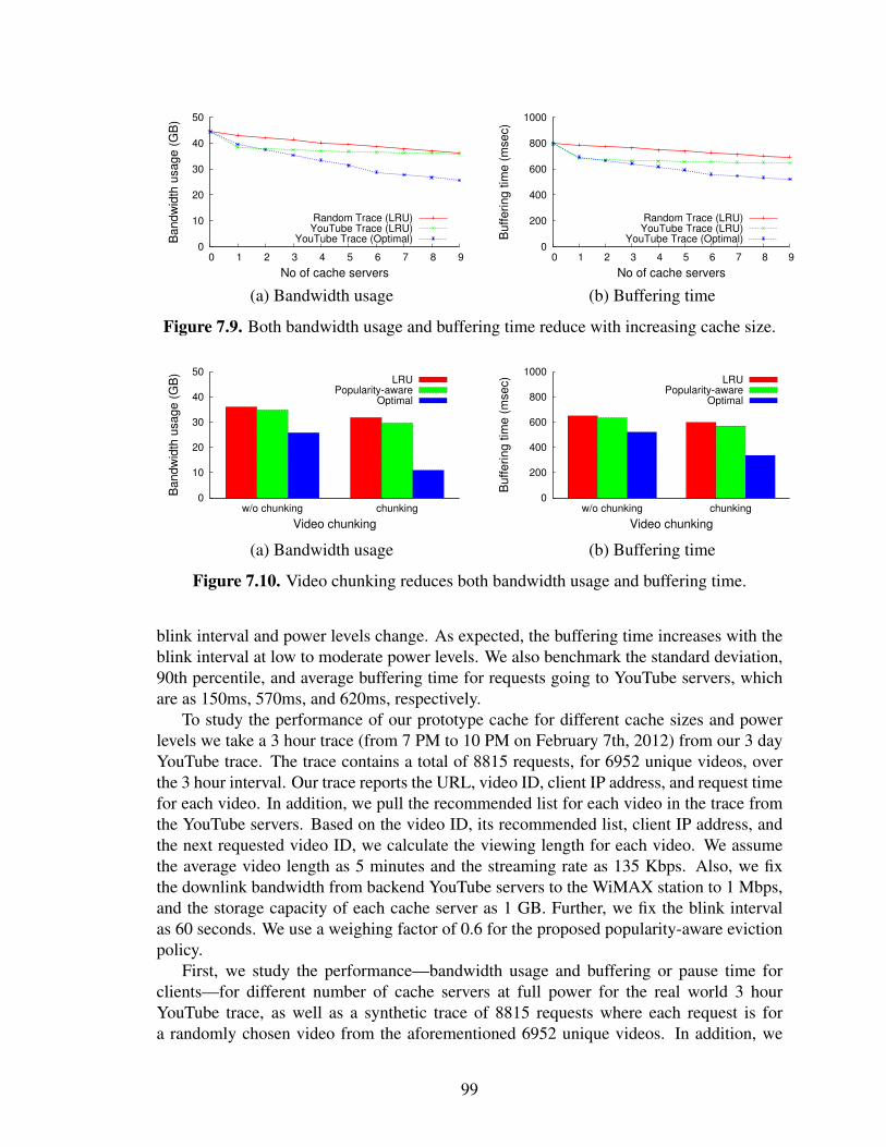
0

10

20

30

40

50

0 1 2 3 4 5 6 7 8 9

Ba

nd

wid

th u

sa

ge

(G

B)

No of cache servers

Random Trace (LRU)YouTube Trace (LRU)

YouTube Trace (Optimal) 0

200

400

600

800

1000

0 1 2 3 4 5 6 7 8 9

Bu

ffe

rin

g t

ime

(m

se

c)

No of cache servers

Random Trace (LRU)YouTube Trace (LRU)

YouTube Trace (Optimal)

(a) Bandwidth usage (b) Buffering time

Figure 7.9. Both bandwidth usage and buffering time reduce with increasing cache size.

0

10

20

30

40

50

w/o chunking chunking

Ba

nd

wid

th u

sa

ge

(G

B)

Video chunking

LRUPopularity-aware

Optimal

0

200

400

600

800

1000

w/o chunking chunkingB

uff

erin

g t

ime

(m

se

c)

Video chunking

LRUPopularity-aware

Optimal

(a) Bandwidth usage (b) Buffering time

Figure 7.10. Video chunking reduces both bandwidth usage and buffering time.

blink interval and power levels change. As expected, the buffering time increases with theblink interval at low to moderate power levels. We also benchmark the standard deviation,90th percentile, and average buffering time for requests going to YouTube servers, whichare as 150ms, 570ms, and 620ms, respectively.

To study the performance of our prototype cache for different cache sizes and powerlevels we take a 3 hour trace (from 7 PM to 10 PM on February 7th, 2012) from our 3 dayYouTube trace. The trace contains a total of 8815 requests, for 6952 unique videos, overthe 3 hour interval. Our trace reports the URL, video ID, client IP address, and request timefor each video. In addition, we pull the recommended list for each video in the trace fromthe YouTube servers. Based on the video ID, its recommended list, client IP address, andthe next requested video ID, we calculate the viewing length for each video. We assumethe average video length as 5 minutes and the streaming rate as 135 Kbps. Also, we fixthe downlink bandwidth from backend YouTube servers to the WiMAX station to 1 Mbps,and the storage capacity of each cache server as 1 GB. Further, we fix the blink intervalas 60 seconds. We use a weighing factor of 0.6 for the proposed popularity-aware evictionpolicy.

First, we study the performance—bandwidth usage and buffering or pause time forclients—for different number of cache servers at full power for the real world 3 hourYouTube trace, as well as a synthetic trace of 8815 requests where each request is fora randomly chosen video from the aforementioned 6952 unique videos. In addition, we

99

0

3

6

9

12

15

Low(20%) Mid.(50%) High(80%)

Bu

ffe

rin

g t

ime

(se

c)

Power

ActivationLoad proportional

Staggered (replication)

0

3

6

9

12

15

Low(10%) Mid.(30%) High(50%)

Bu

ffe

rin

g t

ime

(se

c)

Oscillation from 45% of full power

ActivationLoad proportional

Staggered (replication)

(a) Steady power (b) Oscillating power

Figure 7.11. Buffering time at various steady and oscillating power levels.

0

200

400

600

800

None Top 5 Top 10 Top 15 Top 20

Bu

ffe

rin

g t

ime

(m

se

c)

No of prefetched videos from related list

Figure 7.12. Buffering time decreases as the number of prefetched videos (first chunkonly) from related lists increases.

choose least-recently-used (LRU) cache eviction policy for this experiment; further, videosare not chunked. Figure 7.9 plots the total bandwidth usage and average buffering time forboth random and real traces. We also plot the optimal performance for real traces assumingwe know all requests in advance. The optimal policy always keeps most popular videosin the cache, and never evicts a popular video to store a less popular video (over a giveninterval). As expected, the total bandwidth usage and average buffering time over the 3hour interval decreases as the size or number of servers increases.

Next, to study the benefits of video chunking we measure the performance of three dif-ferent cache eviction policies—LRU, popularity-aware, and optimal—for the 3 hour realtrace at full power and 9 cache servers. Figure 7.10 shows that the performance of Green-Cache’s popularity-aware eviction policy is better (∼ 7%) than that of LRU. Further, videochunking improves (¿ 15%) the performance of all policies as it avoids storing unpopularchunks of popular videos. In all cases, LRU performs worse than others, which motivatesour use of a popularity-aware cache eviction policy and video chunking for all further ex-periments.

7.6.2 Staggered load-proportional blinking

As discussed earlier, the total bandwidth usage over a fixed interval, as long as a re-quest does not go to backend servers for an already cached video, does not depend onthe available power level or blinking and layout policies; it only depends on the cache

100

size and eviction policies. However, buffering time and users’ experiences do depend onthe available power, blinking and layout policies. In this section, we study the effects ofthe power level on the average buffering time, and various optimizations designed to re-duce the buffering time. We use the same 3 hour real YouTube trace, as discussed above,and 9 cache servers for all further experiments. Further, we use video chunking and thepopularity-aware eviction policy for all experiments.

To compare the proposed staggered load-proportional policy with the activation andload-proportional policies from Blink [93], we also implement an activation policy and aload-proportional policy for GreenCache, and integrate them with GreenCache’s popularity-aware eviction policy, video chunking, and popularity-aware migration policy. The activa-tion policy activates or deactivates servers as power varies, whereas the load-proportionalpolicy distributes the power to servers in proportion to their popularity. Similar to the load-proportional policy, the activation policy also migrates popular chunks to active serverswhile deactivating servers due to the drop in the power level. Unlike the proposed stag-gered load-proportional policy, the load-proportional policy from Blink [93] does not repli-cate video chunks because it does not benefit from replication as it activates all servers atthe same time every blink interval.

Figure 7.11(a) shows the average buffering time at different steady power levels. Asexpected, the activation policy performs better than the load-proportional policy at lowpower levels since, unlike the load-proportional policy, the activation policy does not incurthe blinking overhead, which becomes significant in comparison to the active interval atlow power levels. However, at moderate to high steady power levels, the benefit of alarger cache size, albeit blinking, dominates the blinking overhead for real-world traces.Furthermore, the buffering time decreases significantly if first chunks are replicated onall servers. Even at low power levels, replication of initial chunks significantly reducesthe buffering time, while still leveraging the benefits of a larger cache size. Moreover, theperformance of the staggered load-proportional policy remains almost the same at all powerlevels. As video popularity changes infrequently, migration overheads in our experimentsare modest (∼ 2%).

Figure 7.11(b) compares the average buffering time for the above policies at differentoscillating power levels. We oscillate available power every five minutes. Since migrationoverhead of the staggered proportional policy is independent of power level, its perfor-mance remains almost the same at all oscillation levels. However, the activation policyincurs migration overhead whenever the number of active servers decreases. Consequently,the activation policy performs poorly at high oscillation levels, as indicated in the figure.Though replication of initial chunks reduces the buffering time at all power levels, it isprimarily required at low power levels.

Next, we evaluate the benefits of prefetching initial chunks of related videos. As Fig-ure 7.12 indicates, prefetching initial chunks of the top five videos reduces the bufferingtime by 10% as compared to no prefetching. Further, since prefetching more videos doesn’timprove the buffering time, we limit the cache to prefetching only first chunks of top fewvideos from the related list. We choose to prefetch top five videos only in order to strike abalance between the performance gain and prefetching overhead.

101

0

10

20

30

0 30 60 90 120 150 180 0

50

100

150

200

250

Bu

ffe

rin

g t

ime

(se

c)

Po

we

r (w

att

s)

Time (minutes)

PowerActivation

Load proportionalStaggered (replication)

Figure 7.13. Buffering time at various power levels for our combined solar/wind powertrace.

7.6.3 Case study

To experiment with our WiMAX base station using a real WiMAX client, we use aLinux Desktop with Intel Atom CPU N270 processor and 1 GB RAM connected to Tel-tonika USB WiMAX Modem. We disable all network interfaces except the WiMAX inter-face. The desktop connects to the WiMAX base station (NEC Rel.1 802.16eBS), which weconfigure to route all video requests from the desktop to the proxy. We replay the same 3hour YouTube trace on the WiMAX client, but we use real power traces from our solar/winddeployment, as described in the previous section, to power the GreenCache cluster.

Figure 7.13 plots average buffering time, calculated every five minutes, for three blink-ing policies: activation, load proportional, and staggered load proportional with first chunksreplicated. As expected, the performance of all three policies goes down (buffering timegoes up) when the available power drops down, and vice versa. However, the performanceof activation degrades more than that of load-proportional when the available power dropsdown, since the activation policy incurs migration overhead when the number of activeservers decreases. Further, replicating first chunks significantly reduces the buffering timefor the staggered load-proportional policy at all power levels. Since the migration overheadof the staggered load-proportional policy is independent of power levels, its performancedoes not vary much, not even when the available power changes significantly, if first chunksare replicated.

7.7 Related Work

The use of caches to improve the performance of multimedia distribution systems hasbeen studied extensively in the past two decades. [98] gives a general overview on existingmultimedia caching techniques. Due to the vast amount of exiting work in this area, we onlyfocus on the work closely related to our approach, although, to the best of our knowledge,there is no existing work that directly addresses multimedia caches for intermittent power.

Wu et al. [101] were among the first to propose the caching of chunks (segments) of avideo. In contrast to our approach chunks are not equal in size and increase exponentiallywith the distance from the start of the video. The intention of this approach is to combine

102

the number of consecutive chunks that are cached with the popularity of the video. E.g., fora very popular video all chunks would be stored on the cache while for less popular chunksonly a certain number of the initial chunks of the video would be cached. Letting the chunksize grow exponentially has the advantage that the initial chunks of many videos can bestored without occupying too much of the caches storage space. Having only one or severalinitial chunks of a video stored on the cache bears the advantage that a requested video canbe streamed to the client and played out without significant delay. Missing chunks can bestreamed from the server immediately after the initial client request to allow for a smoothplay out. In contrast to the approach presented by Wu et al., we decided for a scheme thatsplits all videos in equal sized chunks (except for the very last chunk) where the completechunk can be transmitted to the client in a period that is equal or smaller than the blinkinterval, assuming a minimum transmission rate.

A more restrictive version of the caching of video chunks is the caching of the firstchunk (prefix) only, which was introduced by Sen et al. [92]. The sole goal of this approachis to reduce the buffer time at the client, since the first chunk can be streamed from thecache much faster than from a remote server. As shown in [90], prefix prefetching cansignificantly improve the viewer’s experience of watching videos and this motivated us toinvestigate how the prefetching approach performs on a multimedia cache for intermittentpower. The results presented above show that prefix prefetching can improve the experienceof a viewer also in the case of a blinking multimedia cache.

As in our current work, trace-based driven simulations are also used in [87] and [103]to investigate the effectiveness of caching for YouTube videos. Both investigations showthat caching of YouTube video can both, on a global and regional level, reduce server andnetwork load significantly. In contrast to the work presented in this chapter, both studiesdo not consider scenarios in which power for the caches is intermittent.

7.8 Conclusion

This chapter presents techniques for optimizing multimedia caches running off intermit-tent renewable energy sources. These caches are important in improving the performanceof “off the grid” cellular towers and base stations, which are increasingly common in de-veloping countries that have both a lack of infrastructure and an unstable grid. We showhow combining a blinking abstraction, which rapidly transitions cache servers between anactive and inactive state, with techniques for chunking (or segmenting) videos, replicatingpopular chunks, and staggering server active intervals improves the performance of thesecaches when compared to standard techniques for powering servers on and off based onavailable power. Our work demonstrates that running multimedia caches off intermittentpower from renewables poses interesting new research problems. Our results show thatGreenCache’s blinking techniques decrease both backhaul bandwidth and client access la-tency compared to existing approaches that simply activate and deactivate servers. In thelatter case, resulting in 3X less buffering (or pause) time by the client watching a video.

103

CHAPTER 8

SUMMARY AND FUTURE WORK

8.1 Thesis Summary

This thesis has explored how distributed systems can be redesigned to run solely onrenewable sources of energy while performing well in spite of significant and frequentvariations in power supply. Further, I have also explored how weather forecasts, whichprovide better predictions than PPF at short to medium time scales ranging from 1 hour to3 days, could be leveraged to predict future solar and wind energy harvesting.

First I analyzed historical weather forecast data from NWS and found that weatherforecasts are a better indicator of future weather than the immediate past. Unlike PPF tech-niques, weather forecasts can also predict sudden changes in weather conditions, whichhappen frequently in many parts of the country including our site. I have designed twosimple empirical models to predict solar and wind energy harvesting based on sky coverand wind speed forecasts from NWS, and shown that predictions based on weather fore-casts outperform predictions based on immediate past by more than 20% in all weatherconditions.

Next I showed how machine learning techniques could be used to better understandrelationships between different weather parameters and how they impact solar intensity.I found that sky cover is not the only parameter that affects solar intensity; rather otherweather parameters, such as temperature, precipitation potential, etc., affect solar intensitytoo. I used the statistical power of machine learning techniques to design better predictionmodels for solar energy harvesting. Unlike previous empirical models, machine learningmodels do not require solar panel and wind turbine deployment to derive region specificmodels. Further, I found that SVM-based prediction models are 27% more accurate for oursite than previous models for solar energy harvesting.

To manage server clusters on renewable sources of energy I proposed an energy ab-straction, called Blink, to regulate the energy footprint of servers in response to varia-tions in power supply. I also designed various blinking policies to coordinate blinkingacross servers in a server cluster. Though each blinking policy allows instant capping ofthe cluster-wide power consumption to the available power, different applications can usedifferent policies to optimize their performance for different workloads. To see how areal-world application can leverage the blinking abstraction I modified Memcached – anin-memory key-value storage system for small chunks of arbitrary data. I showed that areal-world application could be redesigned, with modest complexity, to perform well onintermittent power.

104

I assume Blink provides a general abstraction for regulating energy footprint of servers,which can be used by a range of distributed applications to experiment with intermittentpower constraints. To extend the horizon of the application-agnostic blinking abstractionacross a wide range of real-world applications, I designed and implemented BlinkFS, ablink-aware distributed file system that combines blinking with a power-balanced data lay-out and popularity-based replication/reclamation to optimize I/O throughput and latencyas power varies. I experimented with three distributed applications – Memcache, MapRe-duce, Search Engine – and found that unmodified real-world applications can perform wellin spite of significant and frequent variations in the available power. Moreover, BlinkFSoutperforms existing distributed file systems for both a sustained low power scenario aswell as a highly intermittent power scenario.

Finally, I used the blinking abstraction to design a distributed multimedia cache, calledGreenCache, for intermittent power. I designed several optimization techniques to mini-mize backhaul bandwidth usage while reducing buffering time at all power levels. I alsoanalyzed extensive traces of YouTube videos and used users’ viewing characteristics to de-sign popularity-aware cache eviction and prefetching policies. I found that GreenCache’sstaggered load-proportional blinking policy in combination with a popularity-aware cacheeviction policy results in 3X less buffering (or pause) time by the client compared to anactivation blinking policy, which simply activates and deactivates servers over long periodsas power fluctuates, for realistic power variations from renewable energy sources.

Our results show that a number of real-world applications can leverage the blinkingabstraction to handle intermittent power constraints. Further, many distributed systems canbe redesigned, with modest complexity, to perform well on intermittent power, and thuscan reduce their dependency on dirty fossil fuels and increase renewable energy penetrationwithout sacrificing the performance.

8.2 Future Work

This section introduces some future research directions that can extend the work pre-sented in this thesis.

• Machine Learning Model For Wind Energy Harvesting: As I have discussed inthis thesis, machine learning provides a few powerful techniques to analyze the cor-relation between solar intensity and other weather parameters, and use the forecastsof other parameters to predict solar energy harvesting in the future. We can explorethese techniques to study the correlation between wind speed and other weather pa-rameters, and design a similar prediction model for wind energy forecast based onforecasts of other weather parameters. Further, these techniques could be expandedwell beyond predicting solar and wind energy harvesting. For example, similar tech-niques could be devised to predict spot market prices of electricity in wholesale elec-tricity markets.

• Leveraging Energy Harvesting in Blink-Aware Distributed Systems: In this the-sis, I have designed distributed systems to run on intermittent power, assuming the

105

available power can change unpredictably and we have no knowledge of future en-ergy supply. One can use energy forecast from our energy harvesting predictionmodels and use that knowledge to schedule applications and data migration to furtherimprove the performance of applications running on a blinking cluster. In addition,energy harvesting knowledge could also be used to make energy-purchasing deci-sions in hybrid data centers, running on both renewables and grid energy, that willoptimize the energy budget while satisfying SLAs.

• Leveraging Blinking Abstraction in Grid-Powered Data Centers: Another com-pelling use of intermittent power is continuously operating a data center power deliv-ery infrastructure at 100%. Since data center capital costs are enormous, maximizingthe power delivery infrastructures utilization by operating as many servers as possi-ble is important. However, data centers typically provision power for peak demands,resulting in low utilization. In this case, intermittent power is useful to continuouslyrun a background workload on a set of servers – designed explicitly for intermit-tent power – that always consume the excess power PDUs are capable of delivering.Since the utilization (and power usage) of a data centers foreground workload mayvary rapidly, the background servers must be capable of quickly varying power usageto not exceed the power delivery infrastructures limits. Deciding which applicationsto run on blinking nodes and when to run in order to maximize the overall perfor-mance of the data center is a challenging problem and requires significant researchcontribution.

106

BIBLIOGRAPHY

[1] Southwest Windpower, Inc. AirX Land Owner’s Manual. October, 2002.

[2] J. Apt and A. Curtright. The Spectrum Of Power From Utility-scale Wind Farms AndSolar Photovoltaic. Carnegie Mellon Electricity Industry Center, Technical ReportCEIC-08-04, August 2004.

[3] L. Barroso and U. Holzle. The Case For Energy-Proportional Computing. Computer,December 2007.

[4] P. Corke, P. Valencia, P. Sikka, T. Wark, and L. Overs. Long-duration Solar-poweredWireless Sensor Networks. EmNets, June 2007.

[5] B. Donovan, D. McLaughlin, M. Zink, and J. Kurose. OTGsim: Simulation Of AnOff-the-Grid Radar Network With High Sensing Energy Cost. SECON, June 2008.

[6] P. Dutta, et al. Trio: Enabling Sustainable And Scalable Outdoor Wireless SensorNetwork Deployments. IPSN, April 2006.

[7] E. Ertin, A. Arora, R. Ramnath, and M. Nesterenko. Kansei: A Testbed For SensingAt Scale. IPSN, April 2006.

[8] X. Jiang, J. Polastre, and D. Culler. Perpetual Environmentally Powered Sensor Net-works. IPSN, April 2005.

[9] A. Kansal, J. Hsu, S. Zahedi, and M. Srivastava. Power Management In Energy Har-vesting Sensor Networks. Transactions on Embedded Computing Systems, September2007.

[10] A. Kansal, D. Potter, and M. Srivastava. Performance Aware Tasking For Environ-mentally Powered Sensor Networks. SIGMETRICS Performance Evaluation Review,June 2004.

[11] K. Lin, et al. Heliomote: Enabling Long-lived Sensor Networks Through Solar En-ergy Harvesting. SenSys, November 2005.

[12] M. Minami, T. Morito, H. Morikawa, and T. Aoyama. Solar Biscuit: A Battery-lessWireless Sensor Network System For Environmental Monitoring Applications. INSS,June 2005.

[13] Clemens Moser. Power Management In Energy Harvesting Embedded Systems.Ph.D. Thesis, ETH Zurich, March 2009.

107

[14] C. Moser, D. Brunelli, L. Thiele, and L. Benini. Real-time Scheduling For EnergyHarvesting Sensor Nodes. RTSS, December 2007.

[15] D. Noh, L. Wang, Y. Yang, H. Le, and T. Abdelzaher. Minimum Variance EnergyAllocation For A Solar-powered Sensor System. DCSS, June 2009.

[16] The GENI Project Office. GENI System Overview. The GENI Project Office, Septem-ber 2008.

[17] J. Recas, C. Bergonzini, T. Simunic Rosing, D. Atienza. Prediction and Managementin Energy Harvested Wireless Sensor Nodes. Wireless VITAE, 2009.

[18] M. Ali, B. Al-Hashimi, J. Recas, and D. Atienza. Evaluation and Design Explorationof Solar Harvested-Energy Prediction Algorithm. DATE, March 2010.

[19] J. Taneja, J. Jeong, and D. Culler. Design, Modeling, And Capacity Planning ForMicro-solar Power Sensor Networks. IPSN, April 2008.

[20] C. Vigorito, D. Ganesan, and A. Barto. Adaptive Control For Duty-cycling In EnergyHarvesting-bsed Wireless Sensor Networks. SECON, June 2007.

[21] L. Wang, et al. AdaptSens: An Adaptive Data Collection And Storage Service ForSolar-powered Sensor Networks. RTSS, December 2009.

[22] G. Werner-Allen, P. Swieskowski, and M. Welsh. Motelab: A Wireless Sensor Net-work Testbed. IPSN, April 2005.

[23] Y. Yang, L. Wang, D. Noh, H. Le, and T. Abdelzaher. SolarStore: Enhancing DataReliability In Solar-powered Storage-centric Sensor Networks. MobiSys, June, 2009.

[24] Database of State Incentives for Renewables and Efficiency. http://www.dsireusa.org,2010.

[25] State of California Executive Order S-21-09. http://gov.ca.gov/executive-order/13269, 2009.

[26] Freeing the Grid: Best and Worst Practices in StateNet Metering Policies and Interconnection Procedures.http://www.newenergychoices.org/uploads/FreeingTheGrid2009.pdf, 2009.

[27] N. Cristianini and J. Shawe-Taylor. An Introduction to Support Vector Machines andOther Kernel-based Learning Methods. Cambridge University Press, 2000.

[28] LibSVM: A Library for Support Vector Machines.http://www.csie.ntu.edu.tw/ cjlin/libsvm/, 2011.

[29] I. Jolliffe. Principal Component Analysis. Springer Series in Statistics, 2002.

[30] N. Sharma, J. Gummeson, D. Irwin, and P. Shenoy. Leveraging Weather Forecastsin Energy Harvesting Systems. University of Massachusetts Amherst, Tech. Rep.,September 2011.

108

[31] A. Kansal, J. Hsu, S. Zahedi, and M. Srivastava. Power Management in Energy Har-vesting Sensor Networks. Transactions on Embedded Computing Systems, September2007.

[32] D. Noh, L. Wang, Y. Yang, H. Le, and T. Abdelzaher. Minimum Variance EnergyAllocation for a Solar-powered Sensor System. DCSS, June 2009.

[33] C. Moser. Power Management in Energy Harvesting Embedded Systems. Ph.D.Thesis, ETH Zurich, March 2009.

[34] U.S. Environmental Protection Agency. Report To Congress On Server And DataCenter Energy Efficiency. August 2nd 2007.

[35] Y. Agarwal, S. Hodges, R. Chandra, J. Scott, P. Bahl, and R. Gupta. Somniloquy:Augmenting Network Interfaces To Reduce PC Energy Usage. In Proceedings of theConference on Networked Systems Design and Implementation, pages 365-380, April2009.

[36] Y. Agarwal, S. Savage, and R. Gupta. SleepServer: A Software-Only Approach forReducing the Energy Consumption of PCs within Enterprise Environments. In Pro-ceedings of the USENIX annual technical conference, pages 22-22, June 2010.

[37] F. Ahmad and T. Vijaykumar. Joint Optimization of Idle and Cooling Power in DataCenters while Maintaining Response Time. In Proceedings of the Conference onArchitectural Support for Programming Languages and Operating Systems, pages243-256, March 2010.

[38] H. Amur, J. Cipar, V. Gupta, M. Kozuch, G. Ganger, and K. Schwan. Robust andFlexible Power-Proportional Storage. In Proceedings of the Symposium on CloudComputing, June 2010.

[39] D. Anderson, J. Franklin, M. Kaminsky, A. Phanishayee, L. Tan, and V. Vasudevan.FAWN: A Fast Array Of Wimpy Nodes. In Proceedings of the Symposium on Oper-ating Systems Principles, pages 1-14, October 2009.

[40] L. Breslau, P. Cao, L. Fan, G. Phillips, and S. Shenker. Web Caching And Zipf-like Distributions: Evidence And Implications. In Proceedings of the InternationalConference on Computer Communications, pages 126-134, June 1999.

[41] J. Chase, D. Anderson, P. Thakar, A. Vahdat, and R. Doyle. Managing Energy AndServer Resources In Hosting Centres. In Proceedings of the Symposium on OperatingSystems Principles, pages 103-116, October 2001.

[42] I. Cohen, J. Chase, M. Goldszmidt, T. Kelly, and J. Symons. Correlating Instrumenta-tion Data To System States: A Building Block For Automated Diagnosis And Control.In Proceedings of the Symposium on Operating System Design and Implementation,pages 231-234, December 2004.

109

[43] G. DeCandia, D. Hastorun, M. Jampani, G. Kakulapati, A. Lakshman, A. Pilchin, S.Sivasubramanian, P. Vosshall and W. Vogels. Dynamo: Amazon’s Highly AvailableKey-value Store. In Proceedings of the Symposium on Operating Systems Principles,pages 205-220, October 2007.

[44] K. Fan, Z. Zheng, and P. Sinha. Steady And Fair Rate Allocation For RechargeableSensors In Perpetual Sensor Networks. In Proceedings of the Conference on Embed-ded Networked Sensor Systems, pages 239-252, November 2008.

[45] X. Fan, W. Weber, and L. Barroso. Power Provisioning for a Warehouse-Sized Com-puter In Proceedings of the International Symposium on Computer Architecture,pages 13-23, June 2007.

[46] A. Gandhi, M. Harchol-Balter, R. Das, J. Kephart, and C. Lefurgy. Power Cappingvia Forced Idleness. In Proceedings of the Workshop on Energy-efficient Design, June2009.

[47] P. Gupta. Google To Use Wind Energy To Power Data Centers. In New York Times,July 20th 2010.

[48] R. Kaushik and M. Bhandarkar. GreenHDFS: Towards an Energy-ConservingStorage-Efficient, Hybrid Hadoop Compute Cluster. In Proceedings of the USENIXAnnual Technical Conference, June 2010.

[49] A. Krioukov, P. Mohan, S. Alspaugh, L. Keys, D. Culler, R. Katz. NapSAC: DesignAnd Implementation Of A Power-Proportional Web Cluster. In Proceedings of theWorkshop on Green Networking, August 2010.

[50] K. Lee, O. Bilgir, R. Bianchini, M. Martonosi and T. Nguyen Managing the Cost,Energy Consumption, and Carbon Footprint of Internet Services. In Proceedings ofthe SIGMETRICS Conference, June 2010.

[51] E. Le Sueur and Gernot Heiser. Dynamic Voltage and Frequency Scaling: The Lawsof Diminishing Returns. In Proceedings of the Workshop on Power Aware Computingand Systems, October 2010.

[52] J. Leverich and C. Kozyrakis. On The Energy (In)efficiency Of Hadoop Clusters. InACM SIGOPS Operating Systems Review, 44(1):61-65, January 2010.

[53] I. Goiri, W. Katsak, K. Le, T. Nguyen, and R. Bianchini. Parasol and GreenSwitch:Managing Datacenters Powered by Renewable Energy. In Proceedings of the Confer-ence on Architectural Support for Programming Languages and Operating Systems,March 2013.

[54] D. Meisner, B. Gold, and T. Wenisch. PowerNap: Eliminating Server Idle Power. InProceedings of the Conference on Architectural Support for Programming Languagesand Operating Systems, pages 205-216, March 2009.

110

[55] A. Dan, D.M. Dias, R. Mukherjee, D. Sitaram, and R. Tewari. Buffering and cachingin large scale video servers. In Proceedings of the 40th IEEE Computer Society Inter-national Conference, March 1995.

[56] A. Dan, and D. Sitaram. Multimedia Caching Strategies for Heterogeneous Appli-cation and Server Environments. Multimedia Tools and Applications, 4(3):279-312,May 1997.

[57] A. Dan, and D. Towsley. An Approximate Analysis of the LRU and FIFO BufferReplacement Schemes. SIGMETRICS, January 1990.

[58] A. Dan, and D. Towsley. LRFU: A Spectrum of Policies That Subsumes the LeastRecently Used and Least Frequently Used Policies. IEEE Transactions on Computers,pages 1352 - 1361, December 2001.

[59] R. Miller. Microsoft To Use Solar Panels In New Data Center. In Data Center Knowl-edge, September 24th 2008.

[60] J. Moore, J. Chase, and P. Ranganathan. Weatherman: Automated, Online, AndPredictive Thermal Mapping And Management For Data Centers. In Proceedings ofthe International Conference on Autonomic Computing, pages 155-164, June 2006.

[61] J. Moore, J. Chase, P. Ranganathan, and R. Sharma. Making Scheduling “Cool”:Temperature-Aware Resource Assignment In Data Centers. In Proceedings of theUSENIX Annual Technical Conference, April 2005.

[62] F. Nah. A Study On Tolerable Waiting Time: How Long Are Web Users Willing ToWait? In Behaviour and Information Technology, 23(3), May 2004.

[63] J. Ousterhout, P. Agarwal, D. Erickson, C. Kozyrakis, J. Leverich, D. Mazieres, S.Mitra, A. Narayanan, G. Parulkar, M. Rosenblum, S. Rumble, E. Stratmann, and R.Stutsman. The Case For RAMClouds: Scalable High-performance Storage EntirelyIn DRAM. In ACM SIGOPS Operating Systems Review, 43(5):92-105, December2009.

[64] S. Pelley, D. Meisner, P. Zandevakili, T. Wenisch, and J. Underwood. Power Routing:Dynamic Power Provisioning In The Data Center. In Proceedings of the Conferenceon Architectural Support for Programming Languages and Operating Systems, pages231-242, March 2010.

[65] E. Pinheiro and R. Bianchini. Energy Conservation Techniques for Disk Array-basedServers. In Proceedings of the International Conference on Supercomputing, pages68-78, July 2004.

[66] A. Qureshi, R. Weber, H. Balakrishnan, J. Guttag, and B. Maggs. Cutting The ElectricBill For Internet-scale Systems. In Proceedings of the SIGCOMM Conference, pages123-134, August 2009.

111

[67] P. Ranganathan, P. Leech, D. Irwin, and J. Chase. Ensemble-level Power Manage-ment for Dense Blade Servers. In Proceedings of the International Symposium onComputer Architecture, pages 66-77, June 2006.

[68] S. Shvachko, H. Kuang, S. Radia, and R. Chansler. The Hadoop Distributed File Sys-tem. In Proceedings of the Symposium on Mass Storage Systems and Technologies,pages 1-10, May 2010.

[69] S. Rivoire, M. Shah, P. Ranganathan, and C. Kozyrakis. JouleSort: A BalancedEnergy-efficiency Benchmark. In Proceedings of the SIGMOD Conference, pages365-376, June 2008.

[70] C. Stewart and K. Shen. Some Joules Are More Precious Than Others: ManagingRenewable Energy In The Datacenter. In Proceedings of the Workshop on Power-Aware Computer Systems, October 2009.

[71] I. Stoica, R. Morris, D. Karger, F. Kaashoek, and H. Balakrishnan. Chord: A Scal-able Peer-to-peer Lookup Service For Internet Applications. In Proceedings of theSIGCOMM Conference, pages 149-160, August 2001.

[72] B. Stone. Google’s Next Frontier: Renewable Energy. In New York Times, November28th 2007.

[73] D. Terry, M. Theimer, K. Petersen, A. Demers, M. Spreitzer, and C. Hauser. Man-aging Update Conflicts In Bayou, A Weakly Connected Replicated Storage System.In Proceedings of the Symposium on Operating Systems Principles, pages 172-183,December 1995.

[74] N. Tolia, Z. Wang, M. Marwah, C. Bash, P. Ranganathan, and X. Zhu. DeliveringEnergy Proportionality With Non Energy-proportional Systems: Optimizing The En-semble. In Proceedings of the Workshop on Power-Aware Computer Systems, SanDiego, California, December 2008.

[75] A. Verma, P. De, V. Mann, T. Nayak, A. Purohit, G. Dasgupta, and R. Kothari.BrownMap: Enforcing Power Budget In Shared Data Centers. IBM, Technical ReportRI09016, December 2009.

[76] A. Wolman, G. Voelker, N. Sharma, N. Cardwell, A. Karlin, and H. Levy. On TheScale And Performance Of Cooperative Web Proxy Caching. In Proceedings of theSymposium on Operating Systems Principles, pages 16-31, December 1999.

[77] H. Zeng, C. Ellis, A. Lebeck and A. Vahdat. ECOSystem: Managing Energy As AFirst Class Operating System Resource. In Proceedings of the Conference on Archi-tectural Support for Programming Languages and Operating Systems, pages 123-132,October 2002.

[78] Q. Zhu, Z. Chen, L. Tan, Y. Zhou, K. Keeton and J. Wilkes. Hibernator: Helping DiskArrays Sleep Through the Winter. In Proceedings of the Symposium on OperatingSystems Principles, pages 177-190, October 2005.

112

[79] C. M. Vigorito, D. Ganesan, and A. G. Barto. Adaptive Control of Duty Cycling inEnergy-Harvesting Wireless Sensor Networks. SECON, June 2007.

[80] S. Ganeriwal, D. Ganesan, H. Sim, V. Tsiatsis, M. Hansen, and M. B. Srivastava.Estimating Clock Uncertainty for Efficient Duty-Cycling in Sensor Networks. SenSys,November 2005.

[81] A. Kansal, J. Hsu, S. Zahedi, and M. B. Srivastava. Power management in energyharvesting sensor networks. ACM Transactions on Embedded Computing Systems,2006.

[82] Q. Zhu, Z. Chen, L. Tan, Y. Zhou, K. Keeton and J. Wilkes. Power-Aware StorageCache Management. In IEEE Transactions on Computers, 54(5):587-602, May 2005.

[83] Endace DAG Network Monitoring Interface. http://www.endace.com/.

[84] Stoke solutions: Mobile data offload. http://www.stoke.com/news/pr/2011/pr020911.asp.

[85] Youtube press statistics. http://www.youtube.com/t/press statistics, September 2012.

[86] W. Balshe. Power System Considerations for Cell Tower Applications.http://www.cumminspower.com/www/literature/technicalpapers/PT-9019-Cell-Tower-Applications-en.pdf, 2011.

[87] M. Cha, H. Kwak, P. Rodriguez, Y. Ahn, and S. Moon. I Tube, You Tube, EverybodyTubes: Analyzing the World’s Largest User Generated Content Video System. InIMC, October 2007.

[88] J. Erman, A. Gerber, K. K. Ramadrishnan, S. Sen, and O. Spatscheck. Over theTop Video: The Gorilla in Cellular Networks. In Proceedings of the 2011 ACMSIGCOMM conference on Internet measurement conference, IMC ’11, pages 127–136, New York, NY, USA, 2011. ACM.

[89] J. Guay. India: Forget the Grid, Community Power is Here.http://ourworld.unu.edu/en/india-forget-the-grid-community-power-is-here/, Au-gust 2012.

[90] S. Khemmarart, R. Zhou, L. Gao, and M. Zink. Watching User Generated Videoswith Prefetching. In MMSys, February 2011.

[91] G. P. Office. Open Virtualized WiMAX Base Station Node for Wide-Area WirelesssDeployments. http://groups.geni.net/geni/wiki/WiMAX, June 2011.

[92] S. Sen, J. Rexford, and D. Towsley. Proxy Prefix Caching for xiMultimedia Streams.In INFOCOM, 1999.

[93] N. Sharma, S. Barker, D. Irwin, and P. Shenoy. Blink: Managing Server Clusters onIntermittent Power. In ASPLOS, March 2011.

113

[94] N. Sharma, J. Gummeson, D. Irwin, and P. Shenoy. Cloudy Computing: LeveragingWeather Forecasts in Energy Harvesting Sensor Systems. In SECON, June 2010.

[95] N. Sharma, P. Sharma, D. Irwin, and P. Shenoy. Predicting Solar Generation fromWeather Forecasts Using Machine Learning. In SmartGridComm, October 2011.

[96] N. Sharma, D. Krishnappa, D. Irwin, M. Zink, and P. Shenoy. GreenCache: Aug-menting Off-the-Grid Cellular Towers with Multimedia Caches. In MMSys, February2013.

[97] N. Sharma, D. Irwin, and P. Shenoy. BlinkFS: A Distributed File System for Inter-mittent Power. University of Massachusetts Amherst, Tech. Rep., 2012.

[98] X. Tang, J. Xu, and S. Chanson. Web Content Delivery. Springer, 2005.

[99] N. Tolia, Z. Wang, M. Marwah, C. Bash, P. Ranganathan, and Z. Zhu. DeliveringEnergy Proportionality with Non Energy-Proportional Systems – Optimizing the En-semble. In HotPower, December 2008.

[100] Z. Liu, Y. Chen, C. Bash, A. Wierman, D. Gmach, Z. Wang, M. Marwah, and C.Hyser. Renewable and Cooling Aware Workload Management for Sustainable DataCenters. In SIGMETRICS, June 2012.

[101] K.-L. Wu, P. S. Yu, and J. L. Wolf. Segment-based Proxy Caching of MultimediaStreams. In WWW, 2001.

[102] Q. Xu, J. Huang, Z. Wang, F. Qian, A. Gerber, and Z. Mao. Cellular Data NetworkInfrastructure Characterization and Implication on Mobile Content Placement. InSIGMETRICS, June 2011.

[103] M. Zink, K. Suh, Yu, and J. Kurose. Characteristics of Youtube Network Traffic ata Campus Network - Measurements, Models, and Implications. Elsevier ComputerNetworks, 2009.

[104] AISO (Solar Powered Green Web Hosting). http://www.aiso.net/.

[105] United Nations Conference on Sustainable Development.http://www.uncsd2012.org/.

[106] Google’s Green PPAs: What, How, and Why.http://www.google.com/green/pdfs/renewable-energy.pdf, April 2011.

[107] Dynamic Pricing and Smart Grid, 2011.

[108] MemcacheDB, 2011.

[109] M. Arlitt, C. Bash, S. Blagodurov, Y. Chen, T. Christian, D. Gmach, C. Hyser, N. Ku-mari, Z. Liu, M. Marwah, A. McReynolds, C. Patel, A. Shah, Z. Wang, and R. Zhou.Towards The Design and Operation of Net-zero Energy Data Centers. In ITherm,May 2012.

114

[110] I. Goiri, K. Le, M. Haque, R. Beauchea, T. Nguyen, J. Guitart, J. Torres, and R. Bian-chini. GreenSlot: Scheduling Energy Consumption in Green Datacenters. In SC, April2011.

[111] I. Goiri, K. Le, T. Nguyen, J. Guitart, J. Torres, and R. Bianchini. GreenHadoop:Leveraging Green Energy in Data-Processing Frameworks. In EuroSys, April 2012.

[112] J. Hamilton. Overall Data Center Costs. In Perspectives.http://perspectives.mvdirona.com/, September 18, 2010.

[113] S. Rivoire and M. Shah and and P. Ranganathan. JouleSort: A Balanced Energy-Efficient Benchmark. In SIGMOD, June 2007.

[114] X. Fan and W. Weber and L. Barroso. Power Provisioning for a Warehouse-SizedComputer. In ISCA, June 2007.

[115] J. Dean and S. Ghemawat. MapReduce: Simplified Data Processing on Large Clus-ters. In OSDI, December 2004.

[116] L. Ganesh and H. Weatherspoon and M. Balakrishnan and K. Birman. OptimizingPower Consumption in Large Scale Storage Systems. In HotOS, May 2007.

[117] Dushyanth Narayanan and Austin Donnelly and Antony Rowstron. Write Off-Loading: Practical Power Management for Enterprise Storage. In FAST, February2008.

[118] S. Akoush and R. Sohan and A. Rice and A. Moore and A. Hopper. Free Lunch:Exploiting Renewable Energy for Computing. In HotOS, May 2011.

[119] R. Urgaonkar and B. Urgaonkar and M. Neely and A. Sivasubramaniam. OptimalPower Cost Management Using Stored Energy in Data Centers. In SIGMETRICS,March 2011.

[120] D. Meisner and C. Sadler and L. Barroso and W. Weber and T. Wenisch. PowerManagement of Online Data-Intensive Services. In ISCA, June 2011.

[121] Dennis Colarelli and Dirk Grunwald. Massive Arrays of Idle Disks for StorageArchives. In SC, November 2002.

[122] S. Ghemawat and H. Gobioff and S. Leung. The Google File System. In SOSP,October 2003.

[123] V. Kontorinis, L. Zhang, B. Aksanli, J. Sampson, H. Homayoun, E. Pettis,D. Tullsen, and T. Rosing. Managing Distributed UPS Energy for Effective PowerCapping in Data Centers. In ISCA, June 2012.

[124] J. Koomey. Growth in Data Center Electricity Use 2005 to 2010. In Analytics Press,Oakland, California, August 2011.

[125] L. L. N. Laboratory. U.S. Energy Flowchart 2008, June 2011.

115

[126] J. Leverich and C. Kozyrakis. On the Energy (In)efficiency of Hadoop Clusters. InHotPower, October 2009.

[127] D. Meisner, B. Gold, and T. Wenisch. PowerNap: Eliminating Server Idle Power. InASPLOS, March 2009.

[128] V. Vasudevan, D. Andersen, M. Kaminsky, L. Tan, J. Franklin, and I. Moraru.Energy-efficient Cluster Computing with FAWN: Workloads and Implications. Ine-Energy, April 2010.

[129] A. Verma, R. Koller, L. Useche, and R. Rangaswami. SRCMap: Energy ProportionalStorage Using Dynamic Consolidation. In FAST, February 2010.

116

designing distributed systems for intermittent powernksharma/thesis/thesis.pdf · designing...

Documents