a relationship between external public debt and … · 2019-09-30 · lic debt acts positively and...

A RELATIONSHIP BETWEEN EXTERNALPUBLIC DEBT AND ECONOMIC GROWTH∗

Enrique R. Casares

Universidad Autonoma Metropolitana-Azcapotzalco

Resumen: Se presenta un modelo de crecimiento endogeno con dos bienes, comer-

ciable (manufacturero) y no-comerciable (no-manufacturero). El co-

nocimiento tecnologico domestico es producido unicamente en el sec-

tor comerciable. Este conocimiento se desborda hacia el sector no-

comerciable. El gobierno emite deuda externa para financiar parte de

su gasto en bienes comerciables. La tasa de interes domestica es igual

a la tasa de interes mundial mas la prima de riesgo paıs. El riesgo

paıs depende positivamente del nivel de la deuda publica externa. Los

hogares piden prestado al exterior y tienen una restriccion de credito

externo. Se obtiene, en el estado estacionario, una relacion no lineal

entre la proporcion deuda publica externa a PIB y la tasa de crec-

imiento, en forma de U invertida. Hay evidencia empırica que muestra

la existencia de esta no linealidad entre deuda publica y crecimiento,

tanto para paıses en desarrollo como desarrollados.

Abstract: An endogenous growth model with two goods, tradable (manufactur-

ing) and non-tradable (non-manufacturing) is presented. Domestic

technological knowledge is produced only in the tradable sector. This

knowledge overflows into the non-tradable sector. The government is-

sues external debt to finance part of its spending on tradable goods.

The domestic interest rate equals the world interest rate plus the coun-

try risk premium. The country risk depends positively on the level of

external public debt. Households can borrow abroad and have an ex-

ternal credit constraint. An inverted U-shaped nonlinear relationship

between the external public debt to GDP ratio and the growth rate

is obtained in the steady state. There is empirical evidence showing

the existence of this non-linearity between public debt and growth, for

both developing and developed countries.

Clasificacion JEL/JEL Classification: F21, F36, F43, O41

Palabras clave/keywords: sector comerciable, aprendizaje por la practica, deuda

publica externa, crecimiento economico, tradable sector, learning by doing, exter-

nal public debt, economic growth

Fecha de recepcion: 29 V 2014 Fecha de aceptacion: 24 II 2015

∗ [email protected]

Estudios Economicos, vol. 30, num. 2, julio-diciembre 2015, paginas 219-243

220 ESTUDIOS ECONOMICOS

1. Introduction

External public debt can have nonlinear impacts on economic growth.Thus, at low levels of indebtedness, an increase in the proportion ofexternal public debt to GDP could promote economic growth; how-ever, at high levels of indebtedness, an increase in this proportioncould hurt economic growth. This article studies the non-monotonicrelationship between external public debt and economic growth via amodel of endogenous growth.

The theory of economic growth examines the relationship be-tween external debt and growth using some contributions from inter-national finance. Thus, Krugman (1989) shows the debt relief Laffercurve (with the shape of an inverted U), where the nominal value ofdebt of a country and its actual expected payment are related. Onthe upward segment of the curve, debt and expected payments in-crease because the risk of default is low; in the descending segment,the level of debt increases but expected payments begin to descendbecause the risk of default is very high. He concludes that when acountry is on the descending segment of the curve, the country suf-fers from debt overhang.1 In this situation of debt overhang, externaldebt obligations act as a tax on investment.

Using the above concepts, researchers have studied the effects ofexternal over-indebtedness. Thus, Cohen (1993) extends the modelof endogenous growth of Cohen and Sachs (1986) to formalize therelationship between external-indebtedness and investment.2 Conse-quently, Cohen presents and compares three economic scenarios. Inthe first one, there is free access to the global financial market, andthe rate of investment (and production) is greater than with financialautarky. In the second scenario, there is a credit restriction with softrepayment, and the investment rate is lower than the free access casebut higher than the financial autarky case. In the third one, there is

1 Krugman (1988) defines a debt overhang problem in a country as a situationwhere its debt is greater than the present value of future resource transfers that

creditors expect.2 Cohen and Sachs (1986) develop a model of endogenous growth in which

external debt can be repudiated. Starting without external debt, the economywill have two stages of indebtedness. The first, without restriction to external

credit, is characterized by an increase in the ratio of external debt to product andan initial high growth rate of product, but progressively decreasing. The second

stage, with restricted borrowing, is characterized by a constant ratio of externaldebt to product and by a lower economic growth rate than the growth rates of

the first stage.

A RELATIONSHIP BETWEEN EXTERNAL PUBLIC DEBT 221

a credit restriction with forced repayment, and the investment rate islower than with financial autarky. Therefore, the investment rate risesin the first scenario, before falling in the second and third scenarios.Thus, the relationship between external debt and investment (andgrowth) is non-linear. In addition, Cohen concludes that the thirdscenario would correspond to the concept of debt overhang, whereexternal debt acts as a tax on investment, hurting economic growth.

Moreover, Saint-Paul (1992) shows an endogenous growth modelwith overlapping generations, where an increase in public debt reducesthe growth rate of the economy. Adam and Bevan (2005) develop amodel of endogenous growth with individuals who live two periods.They study various ways to finance public deficits. An increase indomestic public debt slows growth, while an increase in external pub-lic debt, financed in concessional terms, but rationed, helps growth.Aizenman, Kletzer and Pinto (2007) show a model of endogenousgrowth with restrictions in tax revenues and public debt. In gen-eral, they find that the higher the public debt the lower the growth.Finally, Checherita-Westphal, Hallett and Rother (2014) present agrowth model with public capital and debt, where the public deficit isequal to public investment. In their model, the relationship betweendebt and growth is nonlinear. So, in the steady state, the optimaldebt to GDP ratio can be determined where growth is maximized.

In order to study the relationship between external public debtand economic growth, this article presents an endogenous growthmodel for a small open economy.

The economy produces two goods, tradable (manufacturing) andnon-tradable (non-manufacturing). The tradable sector produces do-mestic technological knowledge through learning by doing (Romer,1989). This knowledge is used in the non-tradable good sector. There-fore, in this model there are two learning externalities.3 The govern-ment taxes households with a lump-sum tax to finance spending ontradable goods and interest payments on its external debt, and the dif-ference between these expenditures and tax revenue, if any, is coveredby external public debt. The foreign lenders perceive a country riskthat depends positively on the level of external public debt. More-

3 This model is related to the productive structure of a dependent economywith externalities. For example, Brock and Turnovsky (1994) develop a model

with a tradable capital good and another non-tradable capital good. Turnovsky(1996) presents a model of endogenous growth where physical capital is tradable

and human capital is non-tradable. Korinek and Serven (2010) develop a modelof endogenous growth in which the production of tradable goods generates higher

learning externalities than the production of non-tradable goods.


over, the government collects taxes through another lump-sum taxon households to finance the purchase of non-tradable goods. House-holds consume a constant fraction of their disposable income, andown the two types of capital. They can borrow abroad, subject to aforeign credit constraint. In this article, country risk is fully trans-ferred to the private sector.4 Thus, interest rate parity adjusted bycountry-risk is assumed, and as a result, the interest rate on the twotypes of capital, external private debt and public debt is equal to theworld interest rate plus the country risk premium.

I study how the economy responds, in the steady state, to an in-crease in the proportion of external public debt to GDP and I obtaina nonlinear relationship between the ratio of external public debt toGDP and the growth rate. That is, my results show an inverted U-shaped curve connecting external public debt and economic growth.This nonlinearity is the result of two opposite effects on the growthrate of the economy when the proportion of external public debt toGDP increases. The positive effect is as follows: when the propor-tion of external public debt to GDP increases, the relative price of thenon-tradable good decreases (the real exchange rate depreciates) andthe tradable sector, leader in technological terms, attracts resources.Therefore, the proportion of labor employed in the manufacturingsector increases and the ratio of non-tradable to tradable capital di-minishes, increasing the growth rate of the economy. The negativeeffect is as follows: when the proportion of external public debt to GDP

increases, the country risk premium increases and interest paymentson total external debt increases. Therefore, household disposable in-come falls, the proportion of savings to GDP declines and resources forcapital accumulation decrease, thus the growth rate of the economydecreases.

At a high external public debt to GDP ratio, the economic growththat is stimulated by the depreciation of the real exchange rate andthe attraction of resources towards the tradable sector, is offset bythe exit of resources to the exterior (due to the burden of externaldebt), and the consequent decrease in the savings to GDP ratio.

The results of this paper are related to Cohen (1993) and Cheche-rita-Westphal, Hallett and Rother (2014), where nonlinear relation-ships between debt and growth are also presented, although in theirmodels, the external debt affects economic growth through different

4 Pancrazi, Seoane and Vukotic (2014) show that, for five European economies,the relationship between the sovereign risk premium and the risk premium forprivate loans is negative for the period 2003-2008 and is positive during the crisis

(2008-2011).


channels than those presented here. The result that public spendingon tradable goods leads to a depreciation of the real exchange rate,stimulating the tradable sector, is related, inversely, with Korinek andServen (2010). They affirm that the accumulation of international re-serves (the extension of credit to foreigners for the purchase of domes-tic tradable goods) leads to a depreciation of the real exchange rate,stimulating the tradable sector and triggering the desired learningeffects.

The results I obtained for an economy with endogenous growth,with two goods, two learning externalities, where the external pub-lic debt acts positively and negatively on economic growth, are notpresent in the literature and contribute to a better understanding ofthe relationship between external public debt and economic growth.Moreover, the existence of a maximum level of external public debtmeans that those responsible for public finances should be prudent inhandling external public debt, to avoid high debt levels and preventthe kind of situations that occurred in Latin America in the 1980sand in the European periphery in recent years.

In the empirical literature, there is evidence showing the exis-tence of this non-linearity between public debt and growth, for bothdeveloping and developed countries. Thus, Pattillo, Poirson and Ricci(2002, 2011) study the contribution of the proportion of external debtto GDP to the growth of per capita GDP for 93 developing countriesbetween the years 1969-1998. They find that the contribution of ex-ternal debt (current net value) on growth is nonlinear, in the form ofan inverted U. The critical point, where the contribution of externaldebt to growth becomes negative, is between 35 and 40% of GDP. Thenegative impact of the high level of external debt on growth operatesthrough adverse effects on the formation of physical capital and totalfactor productivity (see Pattillo, Poirson and Ricci 2004). Analyzing55 low-income countries between the years 1970 to 1999, Clements,Bhattacharya and Nguyen (2003) argue that the servicing of externaldebt negatively affects public investment and, indirectly, growth.

Recently, Reinhart and Rogoff (2010) argue that the relation-ship between public debt to GDP ratio and growth for advanced andemerging countries is weak at levels of public debt to GDP ratio lowerthan 90%, but the relationship is negative for ratios greater than90%. Similarly, Caner, Grennes and Koehler-Geib (2010) determinethe critical level, where an increase in average public debt ratio toGDP decreases the average annual growth for developed and develop-ing countries between the years 1980-2008. They conclude that forthe total sample of countries, the threshold stands at 77.1% of GDP.


For developing economies, the critical level is at 64% of GDP. Also,Checherita-Westphal and Rother (2012) show that the relation be-tween public debt to GDP ratio and growth in per capita income hasan inverted U shape, for a sample of 12 countries in the euro area,with data since 1970. The threshold is between 90-100% of GDP,and could even begin at levels of 70-80% of GDP. The main chan-nels through which public debt affects the rate of growth are privatesaving, public investment and total factor productivity. However, ina detailed review of the empirical literature, Panizza and Presbitero(2013) argue that the non-linear relationship between public debt andgrowth, with a threshold of 90% of GDP, is not robust across samples,specifications and estimation techniques.

It is important to mention that in the empirical literature there isalso evidence of a relationship which is always negative between debtand growth; for example, Kumar and Woo (2010) show an inverserelationship between initial public debt and growth of per capita GDP

for advanced and developing economies for the period 1970-2007.The paper is organized as follows. In section 2, I develop an

endogenous growth model of a small open economy. In section 3, Iredefine the model in stationary variables. In section 4, I demonstratethe existence and stability of the steady state, as well as the nonlinearrelationship between external public debt and growth. I present myconclusions in section 5.

2. The economy

In this model, the economy is small, so the world market determinesthe price of the tradable good and the world interest rate. Moreover,there is a country risk that depends positively on the external publicdebt. The tradable and non-tradable goods are produced using phys-ical capital, labor and domestic technological knowledge. For simplic-ity, the tradable sector is the only one that generates domestic tech-nological knowledge through learning by doing. Knowledge overflowsto the non-tradable sector. Capital is specific in both sectors. Therepresentative firm, in both the tradable and the non-tradable sector,maximizes profits taking the externality as given. The governmentimposes two lump sum taxes on households, one to finance spendingon tradable goods and interest payments on the external public debt,and the other to finance the purchase of non-tradable goods. Thegovernment borrows from the rest of the world to purchase tradablegoods. The representative household consumes a constant fraction of


its disposable income. Households can borrow abroad, and have anexternal credit constraint. The total supply of labor is constant, andthere is free mobility of labor between the two productive sectors.

2.1. Production of the tradable good

It is assumed that the production function of the tradable sector isCobb-Douglas:

YT = AT KαT L1−α

T E1 (1)

where YT is the production of the tradable good, AT is a positive pa-rameter of efficiency, KT is the stock of physical capital accumulatedof the tradable good, LT is the labor employed in the sector, α and1−α are the shares of KT and LT , respectively, with 0 < α < 1, andE1 is a learning externality. It is assumed that KT is used only inthe tradable sector.

Domestic technological knowledge is created through learning bydoing in the sector. Therefore, E1 is the external effect of KT inthe production function of the tradable sector. In order to generateendogenous growth, it is assumed that E1 = K1−α

T so the produc-tion function of the tradable sector has constant returns in a broadmeasure of capital (see Romer, 1989).

P wT is defined as the world price of the tradable good, which is

constant and given by the world market. The price of the tradablegood is used as the numeraire (P w

T = 1). Furthermore, rw is definedas the world interest rate, which is constant. I introduce a countryrisk premium on rw. Since this model is an endogenous growth model,I assume that an indicator that measures country risk is the ratio ofexternal public debt to KT , defined as d. The greater the proportiond, the higher the level of country risk. Thus, the model assumes thatd = DG/KT where DG is the external public debt. Since this articleassumes that the country risk is fully transferred to the private sector,a parity of returns adjusted for country risk is assumed. Therefore,the interest rate, r, on domestic assets and external private and publicdebt is:

r = rw + ηd (2)


where η is a positive parameter that reflects country specific factors(see Eicher and Turnovsky, 1999, Eicher and Hull, 2004). Consid-ering that the rate of depreciation of KT is zero, we obtain RT =

P wT

(

r − P wT /P w

T

)

, where RT is the rental price of KT and P wT /P w

T

are the capital gains of KT , with P wT = dP w

T /dt. Considering thatP w

T is the numeraire, the rental price of KT is RT = r. Firms in thetradable sector maximize profits taking the externality as given. Thefirst order conditions are:

wT = AT KT (1 − α)L−αT (3)

RT = r = AT αKα−1T L1−α

T

[

K1−αT

]

= AT αL1−αT (4)

Equation (3) establishes that the wage is equal to the value ofthe marginal product of labor in the tradable good sector. Equation(4) states that the rental price of KT is equal to the marginal productof KT .

2.2. Production of the non-tradable good

With respect to the non-tradable sector, the production function isCobb-Douglas:

YN = ANKβNL1−β

N E2 (5)

where YN is the production of the non-tradable good, AN is a positiveparameter of efficiency, KN is the stock of physical capital accumu-lated from the non-tradable good, LN is the labor employed in thesector, β and 1 − β are the shares of KN and LN , respectively, with0 < β < 1, and E2 is a learning externality. The stock of KN is usedonly in the non-tradable sector.

As the knowledge generated in the tradable sector is a publicgood, there is a spillover effect of knowledge between sectors. Thus,E2 is the contribution of domestic technological knowledge in theproduction of the non-tradable good. Additionally, in order to have


constant returns for a broad measure of capital in the sector, it is

assumed that E2 = K1−βT .

The variable pN is defined as the relative price of the non-trad-able to the tradable good. Considering that the rate of depreciationof KN is zero, the rental price of KN is RN = pN(r− pN/pN), wherepN/pN is the growth rate of pN , or the capital gains of KN . Non-tradable firms maximize profits taking the externality as given. Thefirst order conditions are:

wN = pNANKβNK1−β

T (1 − β) L−βN (6)

RN = pN (r − pN/pN) = pNANβKβ−1N L1−β

N

[

K1−βT

]

(7)

= pNANβKβ−1N K1−β

T L1−βN

Equation (6) states that the wage equals the value of the marginalproduct of labor in the non-tradable sector. Equation (7) is the dy-namic equilibrium condition for KN . Thus, the equation says thatthe rental price of KN is equal to the value of the marginal productof KN .

In models with tradable and non-tradable goods, the real ex-change rate is defined as the level of relative prices of non-tradablegoods in the foreign country in physical terms divided by the levelof relative prices of non-tradable goods in the domestic country inphysical terms. Considering that the level of relative prices of theforeign country is constant, the real exchange rate is inversely relatedto the level of relative prices of non-tradable goods in the domesticcountry in physical terms. Therefore, an increase in pN correspondsto an appreciation of the real exchange rate.

2.3. Government

Regarding the tradable goods, the government spends a certain sumon consumption and interest payment on its external debt. Its spend-ing is financed by a lump sum tax levied on households and by foreign


loans. Consequently, the government budget constraint on the trad-able good is:

DG = rDG + GT − TT (8)

where DG is the external public debt, DG is the increase in public debtover time, rDG is interest payment on the public debt, GT is spendingon consumption on the tradable good, and TT is a lump sum tax.The level of external public debt is measured as a constant fraction,θG, of YT , that is, DG = θGYT , where θG > 0 and DG = θGYT .Furthermore, it is assumed that GT = φT YT ; that is, public spendingon tradable goods is a constant fraction, φT , of the product of thetradable sector, where 0 < φT < 1. Given that the inter-temporalbudget constraint of the government, deducible from equation (8), ismet by the appropriate adjustment of some residual fiscal variable (seeServen, 2007), I assume that the level of TT is adjusted residually.5

Considering the prior definitions given, I find that:

TT = rθGYT + φT YT − θGYT (9)

Regarding the non-tradable goods, the government has an expen-diture on consumption and this consumption is financed by a lumpsum tax charged to households. Therefore, the government budgetconstraint in the non-tradable good is TN = pNGN , where TN is alump sum tax and pNGN is consumption spending in the non-tradablegood. I assume that pNGN = φNpNYN ; that is, public spending onnon-tradable goods is a constant fraction, φN , of the product of thenon-tradable sector, where 0 < φN < 1. Considering the above defi-nitions, we have:

TN = φNpNYN (10)

Therefore, the government only borrows from the rest of theworld for the purchase of tradable goods.

5 Alternatively, a rule of debt stabilization can be postulated, TT =τDG whereτ is the variable rate of adjustment. The end result is the same (see Brauninger

2005 and Heijdra and Ploeg 2002).


2.4. Households

Households own KT and KN , and foreigners own the external debtof the households. The household budget constraint is:

wT LT + wNLN + RT KT + RNKN − TT − TN − rDH (11)

= CT + pNCN + IT + pNIN − DH

where wT LT +wNLN is wage income, RTKT +RNKN is the incomefrom KT and KN , respectively, TT and TN are lump sum taxes, DH

is the external debt of the households, rDH is the interest payment,CT is consumption of the tradable good, CN is consumption of thenon-tradable good, IT = KT is the net investment in KT , IN = KN

is the net investment in KN , and DH is the increase in householddebt through time.

I assume that only a constant and exogenous fraction, θH , ofKT can be used as collateral for loans in the world market, with0 < θH < 1. Therefore, the borrowing constraint is DH = θHKT .Thus, domestic residents own the entire stock of KT , which is partiallyfunded by the world market, and external residents own the debt ofKT (see Barro, Mankiw and Sala-i-Martin, 1995). Moreover, given

that DH = θHKT , one obtains DH = θHKT .Next, I deduce the consumption demands for the tradable and

non-tradable goods. I assume that consumption demands result fromthe maximization of the utility function u = Cγ

TC1−γN subject to the

constraint of the total consumer spending C = CT + pNCN , whereγ and 1 − γ indicate the proportion of the expenditure in CT andCN with respect to aggregated consumption, C, respectively, with0 < γ < 1. Thus, the demands for CT and CN are: CT = γC andpNCN = (1 − γ)C.

For simplicity, I assume that households choose the level of ag-gregate consumption as a constant fraction of disposable income,wT LT +wNLN +RT KT +RNKN −TT −TN − rDH (there is no pos-sibility for inter-temporal choice, which is a limitation of the model).Consequently, I obtain:

C = (1−s)

[

wT LT +wNLN +RT KT +RNKN −TT −TN −rDH

]

(12)


where s is the savings rate and (1 − s) is the consumption rate, sis constant and exogenous, with 0 < s < 1. Note that since TT ,represented by equation (9), is a residual tax, the disposable incomeof the households is decreased by the interest payments on the ex-ternal public debt and by public spending on the tradable good, butincreased by DG, along with public spending on the non-tradablegood, represented by equation (10).

2.5. Equilibrium

First, I deduce the aggregate condition of savings being equal to in-vestment. Substituting wT , wN , RT and RN , equations (3), (4), (6)and (7), in equation (11), I obtain the resource constraint of the econ-omy:

YT +pNYN −TT −TN −rDH = CT +pNCN +IT +pN IN −DH (13)

where YT + pNYN − TT − TN − rDH is equivalent to household dis-posable income. Thus, the aggregated consumption of householdsis:

C = (1 − s) [YT + pNYN − TT − TN − rDH ] (14)

Substituting equation (14) in (13), with C = CT + pNCN , oneobtains:

s [YT + pNYN − TT − TN − rDH ] + DH = IT + pN IN (15)

Equation (15) says that household savings plus the foreign creditextended to households serve to finance capital accumulation.

Next, I obtain the equilibrium conditions of the market of thetradable and non-tradable goods. Since the relative price of the non-tradable good is flexible, the supply of the non-tradable good is alwaysequal to its demand. Therefore, the equilibrium condition for themarket for the non-tradable good is:

pNYN = pNCN + pNGN + pNIN (16)


where pNGN = TN . In order to obtain the equilibrium condition forthe market of the tradable good, equation (16) is substituted into(13), yielding:

YT − TT − rDH = CT + IT − DH (17)

Substituting the government budget constraint, equation (8), inthe above equation results in:

YT − GT − r(DH + DG) + DH + DG = CT + IT (18)

Considering that D = DH + DG, where D is the total externaldebt, and that D = DH + DG, the current account is defined as:

D = rD − NX (19)

where NX is the trade balance. Finally, substituting (19) into (18),one obtains:

YT = CT + GT + IT + NX (20)

The previous equation shows the equilibrium condition for themarket of the tradable good. Regarding the labor market, I assumethat the total labor supply, L, is constant. The equilibrium conditionin the labor market is L = LT + LN .

3. The model in stationary variables

Given that the variables KT and KN show a constant, common rateof growth, it is necessary to define the model variables as station-ary variables, that is, variables that are constant in the steady state.Thus, z = KN/KT is defined as a stationary variable. Furthermore,given that L is constant, it is normalized to one (L = 1). Thus, theequilibrium condition in the labor market is: n + (1 − n) = 1, wheren is the fraction of labor employed in the tradable sector and (1− n)


is the fraction of the labor employed in the non-tradable sector. As nis constant in the steady state, the variable n is also stationary. Sim-ilarly, as the relative price of the non-tradable good must be constantin the steady state, pN is another stationary variable.

Taking into consideration the externalities E1 and E2, the pro-duction functions in stationary variables are:

YT = AT KT n1−α (21)

YN = ANzβKT (1 − n)1−β

(22)

Also, since DG = θGYT , then d = DG/KT = θGAT n1−α. Usingthe equation (2), the rate of interest must be:

r = rw + η θGAT n1−α (23)

The marginal conditions for the tradable sector in stationaryvariables are:

wT = AT KT (1 − α)n−α (24)

r = AT αn1−α (25)

The first order conditions for the non-tradable sector in station-ary variables are:

wN = pNANzβKT (1 − β) (1 − n)−β (26)

r −

pN

pN=

ANβ(1 − n)1−β

z1−β(27)

I assume that α > β, so the tradable sector is more capitalintensive than the non-tradable sector. Turnovsky (1997) shows thatthe dynamic in dependent economies changes when one sector is morecapital intensive than the other.


The static condition of efficient allocation of labor between thetwo sectors is obtained by equating (24) and (26):

AT (1 − α)n−α = pNANzβ(1 − β)(1 − n)−β (28)

This condition says that the value of the marginal product oflabor in both sectors must be equal at all times. With equation (28),the level of pN is:

pN =AT (1 − α) (1 − n)

β

ANzβ (1 − β)nα(29)

Then, the growth rates of KT and KN are obtained in stationaryvariables. Substituting IT = KT , IN = KN and DH = θHKT intoequation (15), and dividing by KT , one obtains:

s [YT + pNYN − TT − TN − rDH ]

KT+ θH

KT

KT=

KT

KT+ pNz

KN

KN(30)

Now, I determine KN/KN in function of KT /KT . Taking loga-rithms and time derivatives of z = KN/KT , one obtains:

z

z=

KN

KN−

KT

KT(31)

As will be apparent later, n is always in a steady state and isconstant. Taking logarithms and time derivatives of equation (29), Iobtain:

z

z= −

1

β

pN

pN(32)

Equating (31) and (32), I have:


KN

KN=

KT

KT−

1

β

pN

pN(33)

Substituting equation (33) into equation (30), I have:

s [YT + pNYN − TT − TN − rDH ]

KT+ θH

KT

KT(34)

=KT

KT+ pNz

[

KT

KT−

1

β

pN

pN

]

Substituting TT and TN , equations (9) and (10), with YT =

AT n1−αKT in the above equation, I obtain:

s [(1 − φT )YT + (1 − φN) pNYN − r (DH + θGYT )]

KT(35)

+ s θGAT n1−α KT

KT+ θH

KT

KT=

KT

KT+ pNz

[

KT

KT−

1

β

pN

pN

]

Finally, substituting DH = θHKT and the production functions,equations (21) and (22), in equation (35) and solving for KT /KT , thegrowth rate of KT is obtained:

KT

KT=

[

1

1 + pNZ − s θGAT n1−α− θH

]{

s[

(1 − φT )AT n1−α (36)

+(1−φN) pNANzβ (1−n)1−β− r(θH +θGAT n1−α)

]

+pNZ

β

pN

pN

}

where r is defined by equation (23). Similarly, I obtain the growth

rate of KN in stationary variables. Substituting IT = KT , IN = KN ,and DH = θHKT into equation (15), dividing by KN , using KT /KT ,


equation (33), substituting TT , equation (9) and TN , equation (10),and using the production functions, equations (21) and (22), I obtain:

KN

KN=

[

1

1 + pNZ − s θGAT n1−α− θH

]{

s[

(1 − φT )AT n1−α (37)

+ (1 − φN ) pNANzβ (1 − n)1−β− r(θH + θGAT n1−α)

]

−

(1 − s θGAT n1−α− θH)

β

pN

pN

}

As n is always in a steady state and is constant, it is possible toshow that the rate of growth of national income, Y = YT + pNYN −

r(

θHKT + θGAT KT n1−α)

, is:

Y

Y=

KT

KT+

pNYN

Y

(

βz

z+

pN

pN

)

(38)

where pNYN/Y is the participation of pNYN in the national income.In the next section, the steady state solution is shown.

4. The steady state and the relationship between externalpublic debt and growth

The steady state solution implies the existence of the equilibrium.Therefore, the growth rates of z, n and pN must be zero in the steadystate, so their levels remain constant. Furthermore, the growth ratesof KT , KN , YT , YN and Y must be equal to a constant rate in thesteady state.

Therefore, with equations (23) and (25), I have:

n∗ =

[

rw

AT (α − η θG)

]1

1−α

(39)

Given that rw, η, θG, AT and α are constant, the level of n∗ is constantin the steady state (steady state levels are denoted with *). It can


be shown that ∂n∗/∂θG > 0; that is, an increase in θG increases n∗.Also, given an increase in θG, the level of n∗ will jump immediatelyto the new steady state level and, thus, n∗ will always be in a steadystate, as mentioned above. With equation (23), the interest rate in

the steady state is r∗ = rw + ηθGAT n∗(1−α).

Using equation (27), with pN = 0 and r∗ = AT αn∗(1−α), I obtain:

z∗ =

[

ANβ

AT α

]1

1−β (1 − n∗)

n∗(1−α)/(1−β)(40)

As z∗ depends on parameters, the level of z∗ is constant in the steadystate. It can be shown that ∂z∗/∂θG = (∂z∗/∂n∗)(∂n∗/∂θG) < 0;that is, an increase in θG decreases z∗.

Using equation (29), and substituting the level of z∗, the relativeprice of the non-tradable good, pN , in the steady state is:

p∗N =

[

AT (1 − α)

AN (1 − β)

] [

AT α

ANβ

]

β

1−β n∗β(1−α)/(1−β)

n∗α(41)

As p∗N depends on parameters, the level of p∗N is constant in thesteady state. Given that α > β, it is possible to demonstrate that∂p∗N/∂θG = (∂p∗N/∂n∗) (∂n∗/∂θG) < 0; that is to say that an increasein θG, causes p∗N to decrease. Thus, for the stationary variables, theexistence of the steady state has been analytically shown.

As in the steady state pN = 0, the growth rate of KT in thesteady state, equation (36), equals the growth rate of KN in thesteady state, equation (37). Similarly, as in the steady state z = 0and pN = 0, the rate of growth of national income, equation (38),

is equal to KT /KT . Also, the growth rate of YT and YN is equal to

KT /KT . Therefore, the steady state growth rate of the economy, g∗,is:

g∗ =[

11+p∗

Nz∗

−s θGAT n∗(1−α)−θH

]

{

s[

(1−φT )AT n∗(1−α) (42)

+(1 − φN ) p∗NANz∗β (1 − n∗)1−β− r∗(θH + θGAT n∗(1−α)

]

}


Given that g∗ depends only on parameters, the level of g∗ isconstant in the steady state.

In order to study the relationship between public debt and growth,I define the proportions of external public debt to GDP and savingsto GDP in the steady state. Since the values of n∗, z∗ and p∗N areknown, the ratio of external public debt to GDP in the steady state,D∗

G,GDP , is

D∗

G,GDP =θGAT n∗(1−α)

[

AT n∗(1−α) + p∗NANz∗β(1 − n∗)1−β

]

As D∗

G,GDP depends on parameters, its level is constant in thesteady state. Moreover, since g∗ is known, the proportion of savingsto GDP in the steady state, S∗

H,GDP , is:

S∗

H,GDP =s[

(1 − φT )AT n∗(1−α) + (1 − φN) p∗NANz∗β(1 − n∗)1−β

]

[

AT n∗(1−α) + p∗NANz∗β(1 − n∗)1−β

]

+s[

−r∗(

θH + θGAT n∗(1−α))

+ θGAT n∗(1−α)g∗]

[

AT n∗(1−α) + p∗NANz∗β(1 − n∗)1−β

]

As S∗

H,GDP depends on parameters, its level is constant in thesteady state. Thus for g∗, D∗

G,GDP and S∗

H,GDP , the existence of thesteady state has also been analytically demonstrated.

Next, I numerically analyze, in the steady state, the relationshipbetween the proportion of external public debt to GDP and the rateof growth of the economy. The values of the parameters α and βare taken from Valentinyi and Herrendorf (2008) where, for the US

economy, they show that the tradable sector is more capital intensive,α = 0.37, than the non-tradable sector, β = 0.32. Given that there isonly net investment, the level of s is the rate of net national saving forOECD economies of 8% relative to national income, s = 0.08 (1980-2012 average, calculated using the world development indicators of the


World Bank). I calculated the levels of public expenditure, the finalconsumption expenditure of the general government sector of OECD

economies, to be 18% of their GDP (1980-2013 average, calculatedusing the world development indicators of the World Bank). Giventhe lack of disaggregated data for expenditure on final consumptionof the general government sector in tradable and non-tradable goods,I opted for φT = 0.10 and φN = 0.18. The level of rw = 0.031 isthe average level of the 10-year Treasury Bonds in the United States(2007-2013 average). As the levels of θH , η, AT and AN dependon the unique characteristics of each economy, they are set only forexplanatory purposes.

Therefore, I present a representative simulation, where the pa-rameter values are: α = 0.37, β = 0.32, s = 0.08, φT = 0.18,φN = 0.18, rw = 0.031, θH = 0.1, η = 0.09, AT = 1.5 and AN = 0.3.In the simulation, I used increasing levels of θG and D∗

G,GDP to clearlyillustrate the effect of the increasing external public debt on economicgrowth. Thus, in figure 1, the relationship between the proportion ofexternal public debt to GDP and the growth rate in the steady state isshown. As shown in figure 1, there is a nonlinear relationship betweenthe external public debt to GDP ratio and the growth rate. That is tosay, there is an inverted U-shaped curve between the proportion of ex-ternal public debt to GDP and growth. A large number of simulationswere carried out and the result holds. This nonlinearity is explainedby two opposite effects on the rate of growth of the economy whenθG and D∗

G,GDP increase. The positive effect is as follows: when θG

and D∗

G,GDP increase, p∗Ndecreases; that is to say, the real exchangerate depreciates. Therefore, the tradable sector employs more laborand accumulates relatively more capital than the non-tradable sec-tor; n∗ increases and z∗ decreases. Given that the tradable sector isthe technological leader, the growth rate of the economy is benefited.The negative effect is as follows: when θG and D∗

G,GDP increase, thecountry risk premium increases, and interest payments on private andpublic debt increase. Thus, national income and the savings to GDP

ratio decrease, and the resources for capital accumulation decrease.Therefore, the growth rate of the economy is damaged.

At point A, in figure 1, θG = 0.0001 and D∗

G,GDP = 0%. Thelevels of the stationary variables are: n∗ = 0.0102, z∗ = 5.217 andp∗N = 14.812. The growth rate in the steady state is 0.63% per annum.The country risk premium is zero and r∗ is 3.1%. The level of savingsto GDP ratio is 6.55%.

Point B, in figure 1, is where the maximum rate of growth isreached by increasing the external public debt to GDP ratio. The


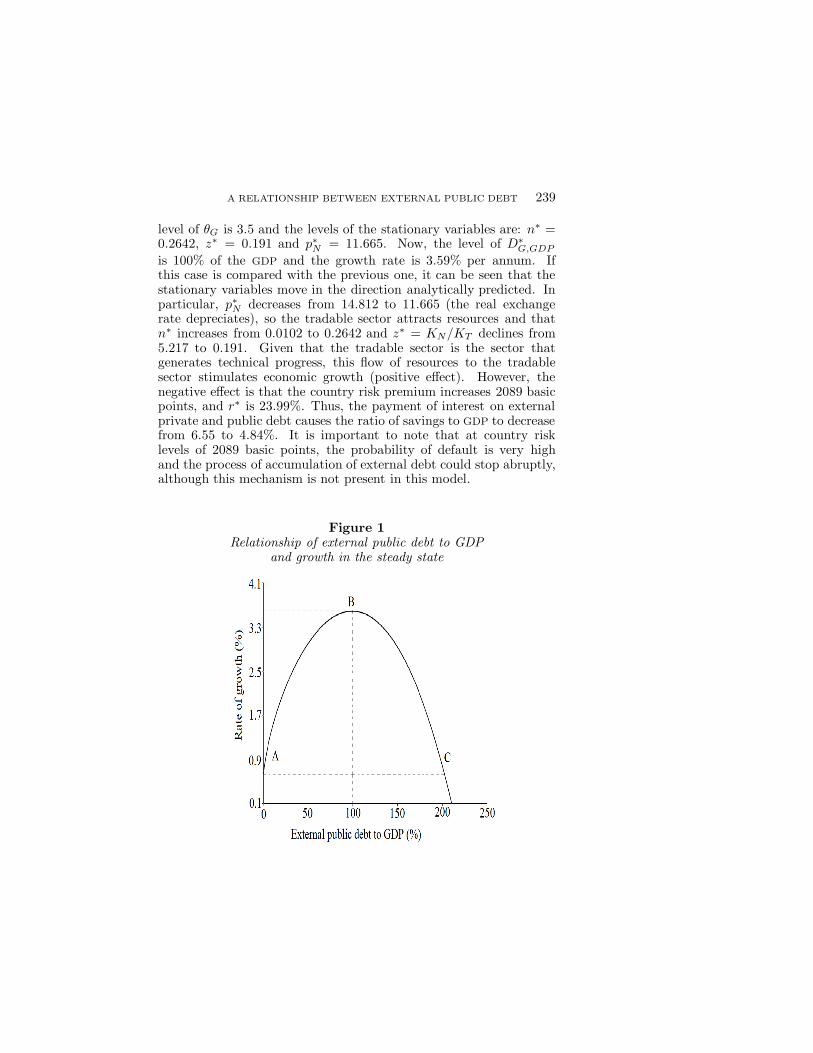
level of θG is 3.5 and the levels of the stationary variables are: n∗ =0.2642, z∗ = 0.191 and p∗N = 11.665. Now, the level of D∗

G,GDP

is 100% of the GDP and the growth rate is 3.59% per annum. Ifthis case is compared with the previous one, it can be seen that thestationary variables move in the direction analytically predicted. Inparticular, p∗N decreases from 14.812 to 11.665 (the real exchangerate depreciates), so the tradable sector attracts resources and thatn∗ increases from 0.0102 to 0.2642 and z∗ = KN/KT declines from5.217 to 0.191. Given that the tradable sector is the sector thatgenerates technical progress, this flow of resources to the tradablesector stimulates economic growth (positive effect). However, thenegative effect is that the country risk premium increases 2089 basicpoints, and r∗ is 23.99%. Thus, the payment of interest on externalprivate and public debt causes the ratio of savings to GDP to decreasefrom 6.55 to 4.84%. It is important to note that at country risklevels of 2089 basic points, the probability of default is very highand the process of accumulation of external debt could stop abruptly,although this mechanism is not present in this model.

Figure 1Relationship of external public debt to GDP

and growth in the steady state


Point C, in figure 1, is where the increase in the external publicdebt to GDP ratio produces the same rate of growth as the case with-out external public debt, g∗ = 0.63%. The corresponding level of θG

is 3.7638 and the levels of the stationary variables are: n∗ = 0.5185,z∗ = 0.067 and p∗N = 11.101. In this case the level of D∗

G,GDP is

202.3% of GDP and the growth rate is 0.63% per annum. If this caseis compared with the case θG = 3.5, it is observed that n∗, z∗ andp∗N move in the direction predicted analytically. In particular, p∗Ndecreases from 11.665 to 11.101 (the real exchange rate depreciateseven further). Therefore, the tradable sector attracts more resources,n∗ increases from 0.2642 to 0.5185, and z∗ = KN/KT decreases from0.191 to 0.067. This flow of resources to the tradable sector stim-ulates economic growth (positive effect). However, the country riskpremium is 3359 basic points and r∗ is 36.6%. Thus the interest pay-ments on private and public external debt reduce disposable incomeand the savings to GDP ratio goes from 4.84 to 0.56% (negative ef-fect). Finally, when the level of D∗

G,GDP is 211% of GDP, the growthrate is zero.

In sum, an inverted U-shaped curve has been presented here, re-lating the external public debt with economic growth. In the upwardsegment of the curve, an increase in the external public debt to GDP

ratio increases growth. However, in the downward segment of thecurve, an increase in the external public debt to GDP ratio decreasesgrowth. Depending on the levels of θH , η, AT and AN (whose valuesdepend on specific factors in each country), the maximum level ofD∗

G,GDP may increase or decrease.In order to study the stability and the transitional dynamics,

equations (32) and (27) are used, yielding:

z + (1/β)(

rw + ηθGAT n1−α)

z = AN (1 − n)1−βzβ

The above equation is a Bernoulli equation, which can be solved by achange of variable v = z1−β and calculating v = (dv/dz)(dz/dt), weobtain:

v + [(1 − β) /β](

rw + θGAT n1−α)

v = (1 − β)AN (1 − n)1−β

where [(1 − β) /β](

rw + θGAT n1−α)

is a positive constant. Also, I

find that (1−β)AN (1 − n)1−β is a positive constant. Thus, when θG


increases, z slowly decreases to its new lower steady state level. Usingequation (29), one can see that at t = 0, pN decreases instantaneouslywhen n jumps, while z stays at the same level. Using equation (32),and since z/z < 0, it can be seen that pN/pN > 0. By all of theabove, at t = 0, it follows that pN decreases and overshoots its newsteady state level. Thus, in the transition, pN rises slowly to its newsteady state level.

5. Conclusions

A model of endogenous growth was developed with two productivesectors, where the tradable sector is the only one that generates do-mestic technical progress. The knowledge generated in the tradablesector is used in the non-tradable sector. The tradable sector andthe non-tradable sector can accumulate physical capital. The gov-ernment spends on tradable goods and on interest payments on itsexternal debt. This expenditure is financed by a lump sum tax leviedon households, and by external public debt. The government alsospends on non-tradable goods, which are financed by a lump sumtax. I assume that the country risk premium increases with the levelof external public debt, and that households borrow from abroad, andface a restriction on foreign credit.

I demonstrate analytically that an increase in the external pub-lic debt to GDP ratio has a positive impact on the tradable sector byreducing the relative price of the non-tradable good. Thus, with thedepreciation of the real exchange rate, the fraction of labor employedin the tradable sector increases and the proportion of non-tradablecapital to tradable capital decreases The relationship between exter-nal public debt and economic growth is shown to have an invertedU-shape. Two opposite effects on the growth rate of the economy ex-plain this nonlinearity between the external public debt to GDP ratioand growth. The positive effect is that, when the external public debtincreases, the relative price of the non-tradable good decreases, so thetradable sector attracts resources, and since the tradable sector is thetechnological leader, the growth rate benefits. The negative effect isthat, when the external public debt increases, the country risk pre-mium increases, and interest payments on the private and public debtincrease. Thus, the household disposable income and the savings toGDP ratio decrease, and the resources for capital accumulation arereduced; consequently, the growth rate is damaged.

Thus, it has been shown that at low levels of indebtedness, anincrease in the external debt to GDP ratio could promote growth;


however, with high levels of indebtedness, an increase in the exter-nal debt to GDP ratio could hurt economic growth. This theoreticalresult resembles certain empirical results that have demonstrated anonlinear relationship between debt and growth.

Furthermore, the inverted U-shaped relationship between exter-nal debt and economic growth indicates the existence of a maximumlevel of external debt, which the policy makers should avoid reaching,in order to prevent situations such as Latin America in the eightiesand the European periphery in recent years.

References

Adam, C.S. and D.L. Bevan. 2005. Fiscal Deficits and Growth in DevelopingCountries, Journal of Public Economics, 89: 571-597.

Aizenman, J., K. Kletzer and B. Pinto. 2007. Economic Growth with Constraintson Tax Revenues and Public Debt: Implications for Fiscal Policy and Cross-Country Differences, NBER Working Paper Series, no. 12750.

Barro, R.J., N.G. Mankiw and X. Sala-i-Martin. 1995. Capital Mobility inNeoclassical Models of Growth, American Economic Review, 85: 103-115.

Brauninger, M. 2005. The Budget Deficit, Public Debt, and EndogenousGrowth,Journal of Public Economic Theory, 7(5): 827-840.

Brock, P.L. and S.J. Turnovsky. 1994. The Dependent-Economy Model withBoth Traded and Nontraded Capital Goods, Review of International Eco-

nomics, 2: 306-325.Caner, M., T. Grennes and F. Koehler-Geib. 2010. Finding the Tipping Point-

When SovereignDebt Turns Bad, The World Bank, Policy Research WorkingPapers, no. 5391.

Checherita-Westphal, C. and P. Rother. 2012. The Impact of High GovernmentDebt on Economic Growth and its Channels: An Empirical Investigation forthe Euro Area, European Economic Review, 56(7): 1392-1405.

Checherita-Westphal, C., A.H. Hallett and P. Rother. 2014. Fiscal SustainabilityUsing Growth-Maximizing Debt Targets, Applied Economics, 46: 638-647.

Clements, B., R. Bhattacharya and T.Q. Nguyen. 2003. External Debt, PublicInvestment, and Growth in Low-Income Countries, International MonetaryFund, IMF Working Papers, no. 249.

Cohen, D. 1993. Low Investment and Large LDC Debt in the 1980’s, American

Economic Review, 83(3): 437-449.Cohen, D. and J. Sachs. 1986. Growth and External Debt Under Risk of Debt

Repudiation, European Economic Review, 30: 529-560.Eicher, T. and L. Hull. 2004. Financial Liberalization, Openness and Conver-

gence, Journal of International Trade & Economic Development, 13: 443-459.


Eicher, T. and S.J. Turnovsky. 1999. International Capital Markets and Non-Scale Growth, Review of International Economics, 7: 171-188.

Heijdra, B. and F. van der Ploeg. 2002. The Foundations of Modern Macroeco-

nomics, Oxford University Press.

Korinek, A. and L. Serven. 2010. Undervaluation Through Foreign ReserveAccumulation. Static Losses, Dynamic Gains, World Bank, Policy Research

Working Papers, no. 5250.Krugman, P. 1988. Financing vs. Forgiving a Debt Overhang, Journal of Devel-

opment Economics, 29: 253-268.——. 1989. Market-Based Debt-Reduction Schemes, in J.A. Frenkel, M.P. Doo-

ley and P. Wickham (eds.) Analytical Issues in Debt, pp. 258-278.Kumar, M.S. and J. Woo. 2010. Public Debt and Growth, International Mone-

tary Fund, IMF Working Papers, no. 174.Pancrazi, R., H.D. Seoane and M. Vukotic. 2014. Sovereign Risk, Private Credit,

and Stabilization Policies , University of Warwick.Panizza, U. and A.F. Presbitero. 2013. Public Debt and Economic Growth in

Advanced Economies: A Survey, Swiss Journal of Economics and Statistics,149(2): 175-204.

Pattillo, C., H. Poirson and L. Ricci. 2002. External Debt and Growth, Interna-tional Monetary Fund, IMF Working Papers, no. 69.

——. 2004. What Are the Channels Through Which External Debt AffectsGrowth?, International Monetary Fund, IMF Working Papers, no. 15.

——. 2011. External Debt and Growth, Review of Economics and Institutions,2: 1-30.

Reinhart, C.M. and K.S. Rogoff. 2010. Growth in a Time of Debt, American

Economic Review, 100(2): 573-578.

Romer, P.M. 1989. Capital Accumulation in the Theory of Long Run Growth,in R. Barro (ed.), Modern Business Cycle Theory, Basil Blackwell.

Saint-Paul, G. 1992. Fiscal Policy in an Endogenous Growth Model, Quarterly

Journal of Economics, 107: 1243-1259.

Serven, L. 2007. Fiscal Rules, Public Investment, and Growth, The World Bank,Policy Research Working Papers, no. 4382.

Turnovsky, S.J. 1996. Endogenous Growth in a Dependent Economy with Tradedand Nontraded Capital, Review of International Economics, 4: 300-321.

——. 1997. International Macroeconomic Dynamic, The MIT Press.Valentinyi, A. and B. Herrendorf. 2008. Measuring Factor Income Shares at the

Sectorial Level, Review of Economic Dynamics, 11: 820-835.

a relationship between external public debt and … · 2019-09-30 · lic debt acts positively and...

Documents