A Proposal forFermilab

To Support the Dark Energy Survey

Design and Development Phase

Submitted by

FermilabJ. Annis, S. Dodelson, B. Flaugher, J. Frieman, S. Kent, H. Lin, L. Hui, J. Peoples,

A. Stebbins, C. Stoughton, D. Tucker, W. Wester

University of Illinois at Urbana-ChampaignR. Brunner, J. Mohr, R. Plante, J. Thaler

Cerro Tololo Inter-American ObservatoryC. Smith, N. Suntzeff

University of ChicagoJ. Carlstrom, J. Frieman, W. Hu, E. Sheldon, R. Wechsler

Lawrence Berkeley National LaboratoryG. Aldering*, N. Roe*

*Contacts for the LBNL Cosmology Group and Microsystems Lab

Proposal Contact Persons

Jim Annis Brenna Flaugherannis@fnal.gov brenna@fnal.govMS 127, Experimental Astrophysics MS 310, Silicon Detector FacilityFermilab FermilabPO Box 500 PO Box 500

Batavia, IL 60510 Batavia, IL 60510

T A B L E O F C O N T E N T S

1. Executive Summary1

2. The Science Program of the Dark Energy Survey4

3. Survey Strategy29

4. The Dark Energy Survey Instrument43

5. Data Management68

6. Project Management Structure and Near Term Goals75

7. The Relationship of the Dark Energy Survey to Other Astrophysics Projects80

8. Conclusions82

Proposal to Fermilab for the Dark Energy Camera

1. Executive Summary

The National Optical Astronomy Observatory (NOAO) has issued an Announcement of Opportunity (AO) for a partnership to develop a major new instrument for the Blanco 4-meter telescope at the Cerro Tololo Inter-American Observatory (CTIO) in Chile. In particular, they encourage construction of an instrument that could exploit either the wide-field capability of the prime focus or the Ritchey-Chrétien focus. We, a group of astrophysicists and physicists from Fermilab, the University of Illinois, the University of Chicago, the Lawrence Berkley National Laboratory (LBNL), and CTIO wish to respond to that AO by submitting a proposal to build an integrated wide-field imaging camera and wide-field corrector for the prime focus of the Blanco 4-meter telescope. Our proposed instrument will have an effective field of view of three square degrees and its focal plane will contain roughly 500 million pixels. These features will give it greater surveying power than any optical or near-infrared camera currently in existence. Our instrument will provide i and z throughputs that are more than a factor of ten greater than those of Mosaic I and II, the existing wide-field cameras used on the Blanco and Kitt Peak National Observatory (KPNO) Mayall 4-meter telescopes. In addition to the proposed instrument, which will include the CCD camera, corrector, and prime focus cage, our collaboration proposes to develop the processing and archiving software for the camera data and to provide the facilities and staff to process, archive, and distribute the processed data from our survey, the Dark Energy Survey. The Dark Energy Survey data and catalogs will be archived and distributed in partnership with NOAO.

Should NOAO select our proposal for the new instrument, we expect that NOAO will award our collaboration up to one-third of the observing time on the Blanco telescope over a five-year period in exchange for delivering the instrument and the software systems. Prior to delivery,, CTIO plans to upgrade the Blanco telescope controls and infrastructure to efficiently accommodate the new instrument. Our collaboration plans to use this awarded time to carry out a survey in four optical passbands (g, r, i and z) over an area of approximately 5000 square degrees. The Dark Energy Survey will provide a powerful probe of the Dark Energy using four complementary measurements of: (i) the abundance and clustering evolution of galaxy clusters, (ii) weak gravitational lensing on large scales, (iii) the evolution of the spatial distribution of galaxies, and (iv) the luminosity distance to type Ia supernova. We select our survey area in the Southern Galactic Cap so that most of the survey area, 4000 square degrees, will be visible from the South Pole; this will allow us to combine our observations with the Sunyaev-Zel’dovich effect survey planned with the South Pole Telescope currently under construction.

The Dark Energy Survey will catalog and provide photometric redshifts for roughly 300 million galaxies out to a redshift beyond one, nearly four times the number of galaxies in and substantially deeper than the Sloan Digital Sky Survey (SDSS), the largest survey to date. Like the SDSS, which has already had a deep impact on science, we expect that our proposed survey will yield rich scientific data and discoveries in a very wide range of topics of interest to astrophysicists, cosmologists, and particle physicists. The SDSS is a very successful international, multi-agency, public-private partnership, and we believe that we can achieve a similar degree of success with the Dark Energy Survey.

1

The Fermilab group proposes to take the responsibility for designing and building the camera, the prime focus cage, and the mechanical and electrical interfaces to the Blanco telescope. The Fermilab group also proposes to design and build the optical corrector in partnership with CTIO. It also proposes to use the skills and resources of the Silicon Detector Facility, because those skills and resources are exceptionally well matched to building a large CCD camera. The LBNL Cosmology Group and Microsystems Group propose to work in collaboration with the Fermilab group to develop and package the CCDs and to design, build, and integrate the front-end electronics chips with the CCDs. The University of Illinois High Energy Physics group proposes to design and build the data acquisition system. These groups, the Camera Team, propose to integrate the camera, the data acquisition system, and the related mechanical, electrical, and communications interfaces with the Blanco into a fully tested and functioning unit at Fermilab prior to shipping the instrument to Cerro Tololo. The Collaboration, with support from the CTIO staff, will mount the instrument on the Blanco prime focus, commission it, and then begin the survey. The Camera Team proposes that their efforts be augmented by the PPD Electrical Engineering Department and Mechanical Support Department.

The University of Illinois Astronomy group, which will be supported by the National Center for Supercomputing Applications (NCSA), proposes to take the leadership of data management and archiving. The Collaboration plans to archive and distribute the data to the scientific community in partnership with NOAO. The University of Chicago group plans to contribute to the science, hardware and software systems, and their major contribution will be to the science software. All participants expect to support the observations and participate in quality assurance of the data and the science analyses. The Collaboration requests some modest support from the Fermilab Computing Division in the areas of data acquisition and data management so that we may take advantage of the experience that the Division gained from building and maintaining the SDSS data acquisition system and from operating the SDSS data processing and data archiving center.

In this proposal, we request that the Director approve the Fermilab participation in the preparation of the proposal that the Dark Energy Collaboration wishes to submit to NOAO by the August 15 proposal deadline. The Fermilab group also requests technical support from the Laboratory in order to produce a preliminary design of the camera and corrector in sufficient detail to enable the Collaboration to demonstrate that the technical performance of the proposed instrument will meet our scientific goals. The preliminary design will include a cost and schedule for the construction and commissioning phases of the Camera, and the Camera Team expects to complete this in May. The Collaboration will augment this support to develop a full cost estimate and schedule for the entire project that they plan to complete in July.

The Camera Team has developed preliminary estimates of the materials and services costs and the labor FTEs for the Dark Energy Camera, and these are included in this proposal. This work has already allowed them to determine that the development and testing of the CCDs and the front-end electronics are the most time critical elements in the schedule. They request sufficient support to initiate a development program that

2

continues through the end of this calendar year on the assumption that we will emerge victorious from the competition. In the event that we are successful, the Collaboration will submit proposals to the Department of Energy Office of Science and the Astronomy Division of the National Science Foundation for funding. The Fermilab group will submit a revised proposal to Fermilab for the support they need to carry out their role in the Collaboration. These proposals will include a plan to obtain the funds to build the instrument and carry out the Dark Energy Survey.

The proposal is organized in chapters as follows: Chapters 2 and 3 describe our Science Goals, the requirements that must be met to achieve them, and the survey strategy that we plan to use to reach them. Chapter 4 describes the Dark Energy Instrument that will make it possible to achieve our goals. Chapter 5 describes our first formulation of the Data Management Plan. Chapter 6 describes the project management structure for the design phase of the project and the relevant prior experience in instrumentation and large surveys. Chapter 7 describes the relationship of the Dark Energy Survey to other relevant astrophysical surveys in which the Dark Energy Collaboration members are engaged and the temporal relationship of our survey to other closely related astrophysics projects. Chapter 8 summarizes the support that the Fermilab Dark Energy team is requesting in this proposal.

3

2. The Science Program of the Dark Energy Survey

What is the nature of the Dark Energy? The National Research Council Report, Connecting Quarks With the Cosmos (2003), identified this as one of the most profound questions about the Universe that are ripe for critical progress in this decade. The Report noted that the dark energy must be probed by multiple, complementary methods with independent systematic errors and different cosmological parameter degeneracies. The Dark Energy Survey is designed to pursue several of the most promising of these methods in the context of a single experiment starting later in this decade and thereby achieve a substantial advance in dark energy precision. In this chapter, we describe the science goals and drivers of the Dark Energy Camera and Survey design.

The Dark Energy Survey data will include accurate fluxes, colors, and shapes of about 300 million galaxies over an area of 5000 square degrees. The fluxes and colors will yield galaxy photometric redshift estimates (described in Section 2.7), a linchpin of several dark energy probes. The survey area is chosen to encompass the Sunyaev-Zel’dovich effect (SZE) cluster survey that will be carried out at the South Pole Telescope (SPT); we will obtain photometric redshifts for the vast majority of SPT clusters, necessary for exploiting the SZE cluster abundance and power spectrum as precision cosmological probes. In particular, we will optically identify and measure accurate photometric redshifts of all clusters in the survey area to a redshift z ~ 1.0 and of a fraction of the clusters extending to z ~ 1.5. We will also measure the shapes of distant galaxies to infer the shear caused by weak gravitational lensing. The weak lensing measurements will calibrate the masses for optically selected clusters out to redshift z ~ 0.7, enabling a purely optical cluster abundance measurement of dark energy parameters in addition to that provided by the SZE. The survey depth and breadth will also enable high-S/N measurement of the weak lensing shear caused by large-scale structure and of the galaxy-shear cross-correlation, each of which provides new constraints on the dark energy. In addition, measurement of the evolution of the angular clustering of galaxies will provide an independent probe of dark energy. Finally, through repeat scanning of selected areas of the survey, we will obtain light-curves for ~1900 Type Ia supernovae and constrain the dark energy through the classical redshift-magnitude relation.

Together, these powerful, complementary techniques will probe the dark energy with unprecedented precision: individually they will probe the dark energy equation of state parameter w (see Sec. 2.1) at the 5-15% level; collectively they can in principle reach the few percent level. It is important to emphasize that these are estimates of statistical errors, assuming constant w, and do not yet include full accounting for systematic errors. Moreover, forecast constraints generally depend on priors assumed for marginalized parameters. As a result, extreme caution must be exercised in comparing the projected cosmological parameter sensitivity of different experiments and methods. More important than the expected statistical precision shown below is the fact that the different methods we will use to probe dark energy are subject to different systematic errors and cosmological parameter degeneracies (see, e.g., Fig. 2.3-2), so their inter-comparison should provide a gauge of the systematic errors and a more robust final result.

As described in this chapter, these science goals can be achieved with a moderately deep (~24th magnitude) survey in four optical passbands, g, r, i, and z. Chapters 3 and 4 show that such a survey can be completed in five years with a new ~500 Megapixel camera

4

with a 3 deg2 field of view on the existing Blanco 4-meter telescope at CTIO. To achieve the requisite depth in the redder passbands within the available survey time, we plan to use thick CCDs with much greater quantum efficiency at long wavelengths than conventional thinned devices

In the following, we highlight the importance of dark energy for fundamental physics and briefly describe the current state of dark energy measurements. We then describe how each of the four methods—cluster counts, weak lensing, galaxy clustering, and supernovae—will constrain the dark energy in the context of our survey. The last section of this chapter describes the expected accuracy of our photometric redshift measurements, a primary factor in determining the science reach of these dark energy methods. An Appendix describes the measurement of the cosmic shear sensitivity of the Survey.

2.1 Evidence for Dark Energy

In 1998, two research groups studying distant Type Ia supernovae independently found direct evidence that the expansion of the Universe is accelerating (Riess et al, 1998, Perlmutter et al 1999), arguably the most important discovery in cosmology since the serendipitous detection of the cosmic microwave background (CMB) radiation by Penzias & Wilson in 1965. According to General Relativity, if the Universe is filled with ordinary matter, the expansion should be slowing down due to gravity. Since the expansion is speeding up, we are faced with two logical possibilities, either of which would have profound implications for our understanding of the fundamental laws of physics: (i) the Universe is filled with a completely new kind of stress-energy with bizarre properties (in particular, negative effective pressure), or (ii) General Relativity breaks down on cosmological scales and must be replaced with a new theory, perhaps associated with extra dimensions. For simplicity, we will subsume both of these possibilities under the general rubric of ‘Dark Energy’, since in both cases the effects on the expansion of the Universe can generally be described by that of an effective fluid with equation of state parameter w = p/ρ < 1/3 (we use units in which the speed of light c = 1 throughout). For example, the dark energy could be the energy of the quantum vacuum, that is, Einstein’s cosmological constant (in which case, w = 1), or it could signal the existence of a new ultra-light particle with mass of order 10-33 GeV or less; in either case, particle physics currently provides no understanding of why the dark energy density should have the value that would explain the acceleration of the Universe.

Since 1998, independent but indirect evidence for dark energy has come from several sources, most notably the combination of the CMB temperature anisotropy pattern—which points to a spatially flat Universe—and the evidence from large-scale structure and galaxy clusters that the density of ordinary matter (mostly dark matter) is about 30% that of a flat Universe. These studies indicate that the dark energy comprises the remaining 70% of the energy density of the Universe, DE 0.7, and that its equation of state parameter w < 0.75 (the exact upper bound depends on priors assumed on other cosmological parameters). In order to pin down the nature of the dark energy and decide between the theoretical alternatives, we need to measure w with greater precision and determine whether and how it evolves with cosmic time. The Dark Energy Survey, in combination with the SPT Survey, is designed to determine w with a statistical precision

5

of ~5% and the dark energy density DE to within 0.01.

6

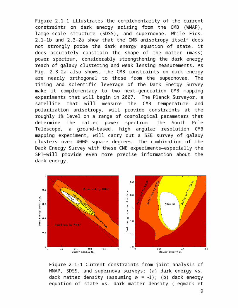
Figure 2.1-1 illustrates the complementarity of the current constraints on dark energy arising from the CMB (WMAP), large-scale structure (SDSS), and supernovae. While Figs. 2.1-1b and 2.3-2a show that the CMB anisotropy itself does not strongly probe the dark energy equation of state, it does accurately constrain the shape of the matter (mass) power spectrum, considerably strengthening the dark energy reach of galaxy clustering and weak lensing measurements. As Fig. 2.3-2a also shows, the CMB constraints on dark energy are nearly orthogonal to those from the supernovae. The timing and scientific leverage of the Dark Energy Survey make it complementary to two next-generation CMB mapping experiments that will begin in 2007. The Planck Surveyor, a satellite that will measure the CMB temperature and polarization anisotropy, will provide constraints at the roughly 1% level on a range of cosmological parameters that determine the matter power spectrum. The South Pole Telescope, a ground-based, high angular resolution CMB mapping experiment, will carry out a SZE survey of galaxy clusters over 4000 square degrees. The combination of the Dark Energy Survey with these CMB experiments—especially the SPT—will provide even more precise information about the dark energy.

Figure 2.1-1 Current constraints from joint analysis of WMAP, SDSS, and supernova surveys: (a) dark energy vs. dark matter density (assuming w = 1); (b) dark energy equation of state vs. dark matter density (Tegmark et al 2003; see also Spergel et al 2003 for an earlier analysis).

2.2 New Probes of Dark Energy

Dark energy affects the history of the cosmic expansion rate, H(z), over the last 10 billion years; this history determines the observables upon which all dark energy probes are based. While supernovae have provided the first direct evidence for dark energy (the observable is the peak apparent brightness as a function of redshift), in the last few years other techniques that complement the supernova method have been undergoing rapid development. The Dark Energy Survey is designed to exploit several of the most promising of these techniques, including supernovae.

7

The first new method involves measuring the number density and clustering of massive clusters of galaxies as a function of their mass and redshift. Galaxy clusters are the largest collapsed structures in the Universe, containing up to hundreds or thousands of individual galaxies. Because the expansion rate of the Universe determines the cosmic volume as a function of redshift as well as the growth rate of density perturbations, the abundance of clusters and its cosmic evolution provide a sensitive new probe of the dark energy equation of state. Realizing this technique is the primary science driver for the Dark Energy Survey.

A major project aimed at the cluster counting technique is now being planned for the South Pole. The South Pole Telescope (SPT, John Carlstrom, U. Chicago, PI), funded by the National Science Foundation, is an $18 million project that will start survey operations in 2007. This project will use the SZE to detect galaxy clusters out to large distances. The SZE is caused by inverse Compton interactions of CMB photons and the hot gas (free electrons) that permeates clusters. These interactions introduce a spectral distortion into the perfect blackbody of the CMB. By precisely mapping the background radiation, the SPT will detect and provide a census of tens of thousands of clusters over a 4000 square degree region south of declination = 30o. Because the SZE signal from a cluster is a measure of the thermal energy in the electron population, it is expected to be a robust indicator of cluster mass.

One advantage of the SZE is that it is a change in the spectral distribution of the CMB rather than a source of emission, so it is unaffected by the cosmological dimming that plagues studies of high-redshift objects. This makes it a cluster selection tool that works extremely well over a wide range of redshifts. However, once clusters are detected in the SZE, one needs another method to determine their redshifts, which are required to measure the cluster abundance and clustering evolution. The most efficient way to obtain cluster redshifts to the desired accuracy is by measuring the magnitudes and colors of the galaxies they contain: all clusters contain a population of luminous red galaxies, and the farther the cluster the redder the galaxies appear. Thus, the SPT survey must be combined, over the same area of sky, with an optical survey in several filters that can measure such color-derived photometric redshifts. Currently, no telescope in the Southern Hemisphere (which can survey the region of sky observable from the South Pole) has an instrument capable of carrying out such a photometric redshift survey with the requisite area and depth on a timescale of a few years.

In addition to providing redshift estimates for the SPT clusters, the Dark Energy Survey will provide an independent cluster counting probe of the dark energy. The cluster counting method depends on having a good estimate of the mass of each cluster. The SZE technique provides one estimate of cluster mass, but optical observations of clusters provide others: the more massive a cluster, the more luminous galaxies it contains and the stronger its gravitational lensing effects on background galaxy images. Current observations indicate that gas-based probes of clusters (i.e., SZE or X-ray signatures) provide more accurate estimates of cluster masses than optical techniques alone. Projection effects that plague both lensing (e.g., Dodelson 2003) and optical mass estimators (e.g., Lin et al 2003) are less problematic (although still present at some level) in SZE surveys. On the other hand, radio emission from the nuclei of galaxies can interfere with SZE cluster selection but does not affect optical cluster finding; moreover, optical and lensing mass estimates do not depend on assumptions about the state of the

8

intracluster gas. Thus, SZE and optical cluster finding and mass estimation are complementary; by coordinating the Dark Energy Survey with the SPT survey, we can cross-check mass estimates and control systematic errors.

A second new technique for probing the dark energy involves weak gravitational lensing: by precisely measuring the shapes of distant galaxies, we can infer how those shapes have been distorted due to their light bending around foreground mass concentrations. The statistical pattern of these distortions—for example, its angular power spectrum—as well as the cross-correlation between foreground lensing galaxies and background galaxy shear, is sensitive to the cosmic expansion history and thus to the dark energy. Weak lensing studies of dark energy require surveys that cover a large area of sky from sites where atmospheric turbulence does not cause excessive blurring of the galaxy images. The site at CTIO is known to have excellent image quality. Third, there is great dark energy leverage available in the power spectra of the spatial distribution of galaxies. The matter power spectrum as a function of wavenumber shows characteristic features, a broad peak as well as baryon wiggles arising from the same acoustic oscillations that give rise to the Doppler peaks in the CMB power spectrum. With the Dark Energy Survey, we will be able to explore the angular galaxy power spectrum in redshift shells out to z~1.1. This approach will provide cosmological information from the shape of the power spectrum transfer function and physically calibrated distance measurements to each redshift shell (Cooray et al 2001, Hu & Haiman 2003).

The fourth approach to dark energy will be to revisit 40 deg2 of the sky every third night, enabling the discovery of and providing light-curves for a sample of 1900 Type Ia supernovae at redshifts 0.3<z<0.8. These SNe will provide relative distance estimates that can be used to constrain the properties of the dark energy—especially when combined with the other three approaches.

These four techniques have very different sources of systematic error from each other. Because we do not yet know the fundamental limitations of these different techniques, and because the problems raised by dark energy are so profound, it is necessary to pursue all of the most promising probes. The Dark Energy Survey does so within a single project. Note that the three new techniques rely on an underlying paradigm for the formation of large-scale structure, based on gravitational instability of cold dark matter in the Universe. Despite the on-going theoretical challenges in fully understanding the formation and evolution of galaxies, recent CMB and large-scale structure data have repeatedly shown that this paradigm is robust, indicating that cosmological parameters can be confidently probed in these new ways.

Below we describe each science component of the Dark Energy Survey in greater detail.

2.3 Galaxy Cluster Studies of the Dark Energy

In recent years, it was recognized that large surveys to redshifts z~1 can measure the galaxy cluster abundance and its evolution and thereby deliver precise constraints on the amount and nature of the dark energy (Wang & Steinhardt 1999, Haiman et al 2001). A cluster survey carried out over large solid angle also constrains cosmology through the spatial clustering of the galaxy clusters. The correlated positions of galaxy clusters (encoded in the cluster power spectrum Pcl(k,z)) reflect the underlying correlations in the

9

dark matter; these correlations contain a wealth of cosmological information, much like the information contained in the CMB anisotropy power spectrum. We plan to use the cluster redshift distribution and the cluster power spectrum as powerful cosmological probes to study the density and nature of the dark energy.

The observed cluster redshift distribution in a survey is the comoving volume per unit redshift and solid angle, d2V/dzdΩ times the comoving density of detected clusters ncom,

0

2222

,1 zdMdnzMfdMzD

zHcznz

dzdVdz

dzdNd

Acom (2.3:1)

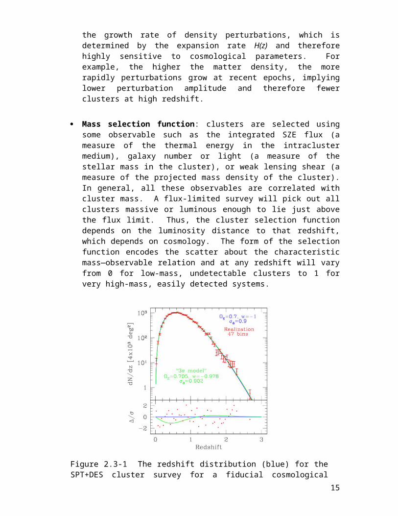
where dn/dM is the cluster mass function, H(z) is the Hubble parameter as a function of redshift, DA(z) is the angular diameter distance, and f(M,z) is the redshift-dependent mass selection function of the survey. Figure 2.3-1 shows a characteristic redshift distribution for the SPT+DES cluster survey. The cosmological sensitivity comes from the three basic elements:

Volume: the volume per unit solid angle and redshift depends sensitively on cosmological parameters and has much in common with a simple distance measurement (such as that given by supernovae).

Abundance Evolution: the evolution of the number density of clusters, (dn/dM)(z), depends sensitively on the growth rate of density perturbations, which is determined by the expansion rate H(z) and therefore highly sensitive to cosmological parameters. For example, the higher the matter density, the more rapidly perturbations grow at recent epochs, implying lower perturbation amplitude and therefore fewer clusters at high redshift.

Mass selection function: clusters are selected using some observable such as the integrated SZE flux (a measure of the thermal energy in the intracluster medium), galaxy number or light (a measure of the stellar mass in the cluster), or weak lensing shear (a measure of the projected mass density of the cluster). In general, all these observables are correlated with cluster mass. A flux-limited survey will pick out all clusters massive or luminous enough to lie just above the flux limit. Thus, the cluster selection function depends on the luminosity distance to that redshift, which depends on cosmology. The form of the selection function encodes the scatter about the characteristic mass—observable relation and at any redshift will vary from 0 for low-mass, undetectable clusters to 1 for very high-mass, easily detected systems.

10

Figure 2.3-1 The redshift distribution (blue) for the SPT+DES cluster survey for a fiducial cosmological model with DE = 0.7, w = 1, and power spectrum amplitude 8 = 0.9. A particular realization of the model appears with red points and error bars. The green model can be excluded with 3σ confidence using a likelihood analysis of this data. The lower panel shows the deviations between the 3σ model and the fiducial model as a function of redshift in units of ν=Δ/σ.

The cosmological sensitivity of the cluster power spectrum arises primarily because there are features—including a break—in the power spectrum that depend on the matter and baryon densities. These features provide a standard ruler, calibrated by the CMB power spectrum. By measuring the cluster angular power spectrum in a redshift bin, one measures the angular scale of these features. Comparing the angular and physical scale of these features provides direct angular diameter distance information to that redshift (Cooray et al 2001). The cosmological constraints from the cluster power spectrum are independent of those from the cluster redshift distribution; taken together, they constrain cosmology in a very robust manner (Majumdar & Mohr 2003b, Lima & Hu 2004).

Several crucial components make possible precision studies of dark energy using galaxy cluster surveys. First, the formation and evolution of dark matter halos is well-understood theoretically and well-tested using N-body simulations of structure formation (Jenkins et al 2001, Hu & Kravtsov 2002, Linder & Jenkins 2003). Second, special-purpose surveys must be designed to cleanly select clusters over a large range of mass and redshift—survey completeness and contamination must be well understood when analyzing the cluster redshift distribution. Third, photometric redshift estimates must be available for large numbers of clusters—this drives the synergy between the SPT and DES surveys. Finally, a mass—observable relation must exist that can tie observable cluster properties (such as the SZE flux or the galaxy light) to the underlying halo mass. The combination of the DES and SPT surveys bring all these ingredients together, making it possible to deliver robust constraints on the dark energy from a sample of ~20,000 clusters.

11

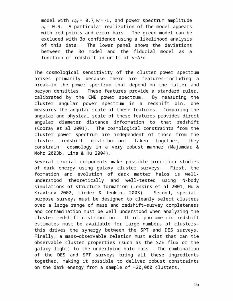
Figure 2.3-2 Forecasts of the constraints on the dark energy equation of state parameter w, the dark energy density parameter E, and the matter density parameter m for the SPT+DES galaxy cluster survey (blue). For comparison, forecasts for SNAP supernovae (green; Perlmutter & Schmidt 2003), current constraints from WMAPext (black; Spergel et al 2003), and forecasts for Planck polarization (red) are shown. The cluster constraints in the left panel either assume a flat universe (solid blue) or solve for geometry and w simultaneously (dashed blue). The constraints arise from the cluster power spectrum, the cluster redshift distribution (assumed distributed uniformly out to z =1), and 100 cluster mass measurements each accurate at the 30% level (1σ). Note that only the SNAP constraint includes an estimate of systematic error.

Figure 2.3-2 shows forecasts for the dark energy constraints from the SPT+DES cluster survey, compared with projected SNAP supernovae and existing and projected CMB constraints. The complementary parameter degeneracies underscore the gains one can achieve by carrying out both cluster surveys and supernova distance measurements, as we plan to do in the Dark Energy Survey. The cluster mass measurements will come from a combination of weak lensing constraints directly from the Dark Energy Survey, deep pointed X-ray observations with Chandra or XMM-Newton, and perhaps through cluster dynamical estimates arising from spectroscopic studies of a subset of the clusters. We emphasize that these forecasts include survey self-calibration: the mass—observable relation and its evolution are extracted from the survey directly (Majumdar & Mohr 2003a,b; Hu 2003, Lima & Hu 2004). The precision of cosmological constraints suffers when one requires self—calibration, but the accuracy is improved by eliminating biases introduced by theoretically driven assumptions about the expected form and evolution of the mass—observable relations. Put another way, the constraints with self-calibration do incorporate an estimate of the effects of a major source of systematic error in the cluster measurements.

In calculating the forecasts shown above we have reserved considerable cosmological information for cross-checking our constraints. As shown in Equation 2.3:1, the redshift distribution involves an integral over the mass function. Using in addition the shape of the mass function directly would improve the cosmological constraints (Hu 2003), but with the approach outlined here we can, at the end of the analysis of the redshift

12

distribution and cluster power spectrum, predict the cluster mass function as a function of redshift. A direct comparison of the theoretical mass functions for the best-fit cosmology and the observed mass functions derived from the survey (in essence, the observed luminosity functions, which can be converted to a mass function using the parameters of the mass—observable relation) will indicate the level of self-consistency—and effectively the level of accuracy—of our analysis. These multiple, independent sources of information from a cluster survey make it a particularly powerful probe of the dark energy.

Finally, we note that the constraints shown here and below assume that the dark energy equation of state parameter w is constant in time; if w evolves, then the corresponding constraints on its present value, w0, are generally less stringent. On the other hand, it has been suggested (Battye and Weller 2003) that the SPT+DES cluster abundance, in conjunction with external determination of the mass power spectrum normalization, can provide constraints on the evolution of w that complement those that will come from SNAP.

2.3.1 Optical Cluster Finding and Mass Estimates

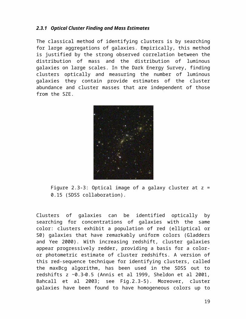
The classical method of identifying clusters is by searching for large aggregations of galaxies. Empirically, this method is justified by the strong observed correlation between the distribution of mass and the distribution of luminous galaxies on large scales. In the Dark Energy Survey, finding clusters optically and measuring the number of luminous galaxies they contain provide estimates of the cluster abundance and cluster masses that are independent of those from the SZE.

Figure 2.3-3: Optical image of a galaxy cluster at z = 0.15 (SDSS collaboration).

Clusters of galaxies can be identified optically by searching for concentrations of galaxies with the same color: clusters exhibit a population of red (elliptical or S0) galaxies that have remarkably uniform colors (Gladders and Yee 2000). With increasing redshift, cluster galaxies appear progressively redder, providing a basis for a color- or photometric estimate of cluster redshifts. A version of this red-sequence technique for identifying

13

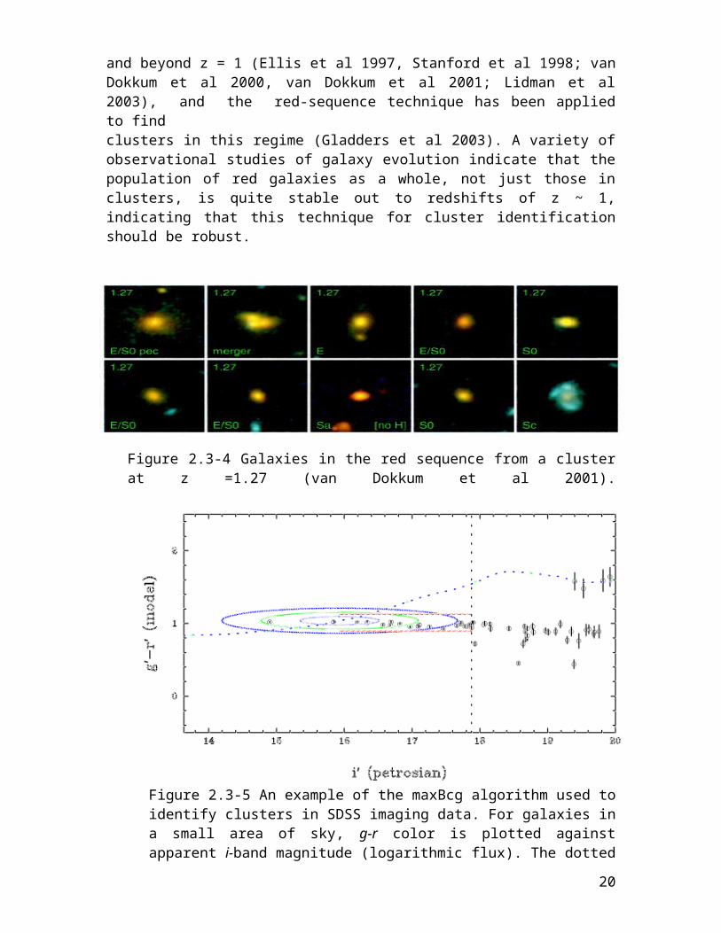
clusters, called the maxBcg algorithm, has been used in the SDSS out to redshifts z ~0.30.5 (Annis et al 1999, Sheldon et al 2001, Bahcall et al 2003; see Fig.2.3-5). Moreover, cluster galaxies have been found to have homogeneous colors up to and beyond z = 1 (Ellis et al 1997, Stanford et al 1998; van Dokkum et al 2000, van Dokkum et al 2001; Lidman et al 2003), and the red-sequence technique has been applied to findclusters in this regime (Gladders et al 2003). A variety of observational studies of galaxy evolution indicate that the population of red galaxies as a whole, not just those in clusters, is quite stable out to redshifts of z ~ 1, indicating that this technique for cluster identification should be robust.

Figure 2.3-4 Galaxies in the red sequence from a cluster at z =1.27 (van Dokkum et al 2001).

Figure 2.3-5 An example of the maxBcg algorithm used to identify clusters in SDSS imaging data. For galaxies in a small area of sky, g-r color is plotted against apparent i-band magnitude (logarithmic flux). The dotted curve shows the expected locus of the most luminous galaxies found in clusters, with redshift increasing along the curve. This cluster is at z =0.1. Ellipses indicate the 1, 2, 3 expectation values for the most luminous galaxy in a cluster at z =0.11, while the vertical dotted line shows the luminosity limit used for the count of red cluster galaxies, Nred.

14

For the SPT survey, the observable used to statistically estimate cluster mass is the SZE flux. For optically selected clusters, one can use, e.g., total galaxy luminosity (e.g., Bahcall et al 2003, Lin et al 2004); for the remainder of this discussion, we will instead adopt the number of red galaxies above a limiting luminosity, Nred, as the optical mass estimator, since it is straightforward to measure with the maxBcg cluster finding technique (see Fig. 2.3-5).

Weak lensing measurements provide a method for calibrating the relation between Nred and cluster mass (see, e.g., Fig. 2.4-2). To obtain high signal to noise, one stacks many clusters of a given Nred and photometric redshift interval and determines the mean tangential shear profile, a technique used on a sample of early SDSS data by Sheldon et al (2001). The mass scalings derived from this method agree very well with those derived from spectroscopic velocity dispersions (McKay et al 2004), an important cross-check on the method. The Dark Energy Survey will allow us to build weak lensing vs. Nred scaling relations out to z =0.7.

Figure 2.3-6 A realization of the cluster redshift distribution from the Hubble Volume N-body simulation. The three curves show the distribution for different mass bins, where M is the cluster mass in units of solar mass. The red curve corresponds roughly to the detection mass threshold for SPT clusters (1014 Msun), while optical imaging can detect clusters down to lower masses, similar to that indicated by the black curve (1013.5 Msun or Nred = 10).

15

2.4 Weak Gravitational Lensing and Dark Energy

The bending of light by foreground mass concentrations shears the images of distant source galaxies. Dense mass concentrations such as galaxy clusters induce a coherent tangential shear pattern that can be used to reconstruct their surface mass densities. Larger scale structures with lower density contrast also generate correlated shear, but with lower amplitude—in this case one studies the shear pattern statistically, a method known as cosmic shear or shear-shear correlations. Since the foreground dark matter is associated to large degree with foreground galaxies, one can also measure the angular correlation between foreground galaxy positions and source galaxy shear, a technique known as galaxy-shear correlations or galaxy-galaxy lensing.

These weak lensing techniques provide powerful probes of the dark energy in the context of our proposed Survey: the shear-shear and galaxy-shear correlations depend on and therefore constrain the dark energy density and equation of state. In addition, as noted above, lensing provides statistical cluster mass estimates that can cross-check SZE, X-ray, and galaxy-number-based mass estimators. While shear-shear and galaxy-shear correlations were detected for the first time several years ago, the Dark Energy Survey, with its wide area coverage, depth, and photometric redshift information, will fully exploit the dark energy sensitivity of these techniques.

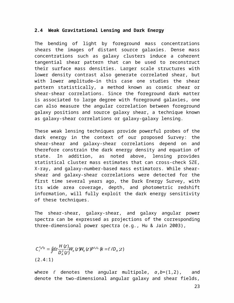
The shear-shear, galaxy-shear, and galaxy angular power spectra can be expressed as projections of the corresponding three-dimensional power spectra (e.g., Hu & Jain 2003),

);/()()()()(

2 zDkPzWzWzDzHdzC A

ssba

A

bxaxba (2.4:1)

where denotes the angular multipole, a,b=(1,2), and denote the two-dimensional angular galaxy and shear fields, and and respectively denote the three-dimensional galaxy (g) and mass (m) density fluctuation fields at redshift z. The weight functions W encode information about the galaxy redshift distribution and about the efficiency with which foreground masses shear background galaxies as a function of their respective distances.

The dark energy density and equation of state affect these angular power spectra through the distance and weight factors and through the redshift- and scale-dependence of the three-dimensional power spectra , , and . For a given set of cosmological parameters, the matter power spectrum can be accurately predicted from N-body cosmological simulations; the shape (scale-dependence) of is also well constrained on large scales by WMAP data on the CMB anisotropy. In addition to cosmology, the power spectra involving galaxies, and , require a model for the bias, that is, for how luminous galaxies are distributed with respect to the dark matter. We describe the bias in terms of the ‘halo model’, with parameters that determine how galaxies occupy dark matter halos; this model is physically motivated and accurately reproduces the results of N-body simulations that include gas dynamics.

16

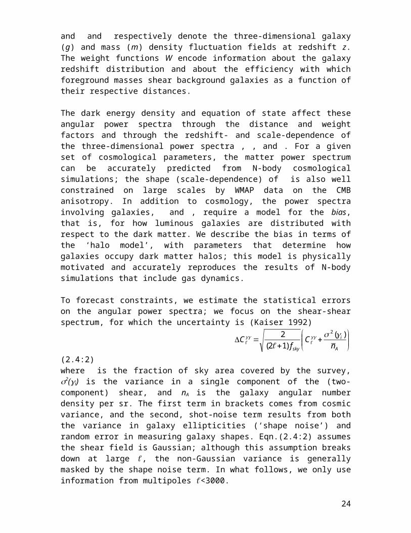
To forecast constraints, we estimate the statistical errors on the angular power spectra; we focus on the shear-shear spectrum, for which the uncertainty is (Kaiser 1992)

A

i

sky nC

fC )(

)12(2 2

(2.4:2)

where is the fraction of sky area covered by the survey, 2(i) is the variance in a single component of the (two-component) shear, and nA is the galaxy angular number density per sr. The first term in brackets comes from cosmic variance, and the second, shot-noise term results from both the variance in galaxy ellipticities (‘shape noise’) and random error in measuring galaxy shapes. Eqn.(2.4:2) assumes the shear field is Gaussian; although this assumption breaks down at large , the non-Gaussian variance is generally masked by the shape noise term. In what follows, we only use information from multipoles <3000.

Eqn. (2.4:2) indicates that weak lensing places a premium on maximizing the survey sky coverage and the surface density of source galaxies with measurable shapes. Following the Appendix (Section 2.8), we use a fiducial effective source galaxy density n per square arcminute, and median source redshift 0.7. We note that n here is smaller than the actual galaxy source density in the Survey, because it includes weighting due to measurement error, point-spread-function (PSF) dilution, and shear polarizability. In comparison to the CFHT Legacy Survey, the signal to noise on the shear variance for the Dark Energy Survey should be larger by a factor of three

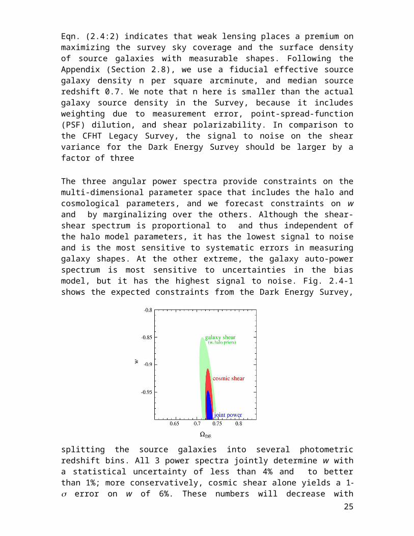
The three angular power spectra provide constraints on the multi-dimensional parameter space that includes the halo and cosmological parameters, and we forecast constraints on w and by marginalizing over the others. Although the shear-shear spectrum is proportional to and thus independent of the halo model parameters, it has the lowest signal to noise and is the most sensitive to systematic errors in measuring galaxy shapes. At the other extreme, the galaxy auto-power spectrum is most sensitive to uncertainties in the bias model, but it has the highest signal to noise. Fig. 2.4-1 shows the expected constraints from the Dark Energy Survey, splitting the source galaxies into several photometric redshift bins. All 3 power spectra jointly determine w with a statistical uncertainty of less than 4% and to better than 1%; more conservatively, cosmic shear alone yields a 1- error on w of 6%. These numbers will decrease with improved priors from Planck.

Figure 2.4-1 68% CL constraints on w and . Red: shear-shear correlations; green:

17

galaxy-shear correlations with halo model parameters constrained by foreground galaxy auto-correlations; blue: joint constraints from all three power spectra.

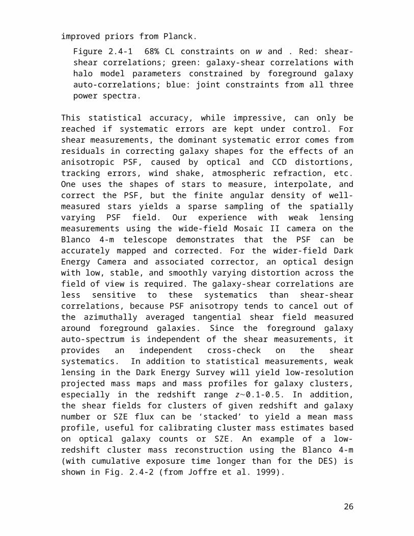
This statistical accuracy, while impressive, can only be reached if systematic errors are kept under control. For shear measurements, the dominant systematic error comes from residuals in correcting galaxy shapes for the effects of an anisotropic PSF, caused by optical and CCD distortions, tracking errors, wind shake, atmospheric refraction, etc. One uses the shapes of stars to measure, interpolate, and correct the PSF, but the finite angular density of well-measured stars yields a sparse sampling of the spatially varying PSF field. Our experience with weak lensing measurements using the wide-field Mosaic II camera on the Blanco 4-m telescope demonstrates that the PSF can be accurately mapped and corrected. For the wider-field Dark Energy Camera and associated corrector, an optical design with low, stable, and smoothly varying distortion across the field of view is required. The galaxy-shear correlations are less sensitive to these systematics than shear-shear correlations, because PSF anisotropy tends to cancel out of the azimuthally averaged tangential shear field measured around foreground galaxies. Since the foreground galaxy auto-spectrum is independent of the shear measurements, it provides an independent cross-check on the shear systematics. In addition to statistical measurements, weak lensing in the Dark Energy Survey will yield low-resolution projected mass maps and mass profiles for galaxy clusters, especially in the redshift range z0.1-0.5. In addition, the shear fields for clusters of given redshift and galaxy number or SZE flux can be ‘stacked’ to yield a mean mass profile, useful for calibrating cluster mass estimates based on optical galaxy counts or SZE. An example of a low-redshift cluster mass reconstruction using the Blanco 4-m (with cumulative exposure time longer than for the DES) is shown in Fig. 2.4-2 (from Joffre et al. 1999).

Figure 2.4-2 Reconstructed projected mass map for the z =0.05 cluster Abell 3266 superposed on a R-band image from the Blanco 4-m telescope. Contours are significance levels, and the image is 44 arcmin on a side; the galaxy source density used to reconstruct the mass map was 15 per arcmin.

18

2.5 Galaxy Angular Clustering

The Dark Energy Survey (DES) will deliver a sample of over 300 million galaxies extending well beyond a redshift of one. On large scales, galaxy clustering and its evolution should reflect the gravitational dynamics of the underlying dark matter distribution. The ratio between the galaxy and dark matter power spectra can be described by a redshift-dependent bias factor, b(z), that is theoretically expected to be scale-independent on large scales, although its amplitude does depend on the type (e.g., luminosity, color) of galaxy being studied. In the linear regime, we can write the galaxy power spectrum as

zbpzgpkTkkP jin

gal222 ;; , (2.5:1)

where the initial dark matter power spectrum from the early Universe nk ,

T k is the scale-dependent transfer function for dark matter perturbations,

g z is the scale-independent perturbation growth function, and the pi remind us that these functions depend explicitly on cosmological parameters.

We will measure the galaxy angular power spectrum within photometric redshift bins to probe the dark energy. The angular power spectrum within a redshift shell can be written as

Cgali (l) k 2dk

0

2

f i2 l,k Pgal k , (2.5:2)

where

f i l,k is the Bessel transform of the radial selection function for redshift shell i (Tegmark et al. 2002, Dodelson et al. 2002).

The transfer function has a characteristic break on a physical scale corresponding to the horizon size at matter-radiation equality, determined by the mean dark matter density, as well as small wiggles associated with the effects of baryon acoustic oscillations on the dark matter distribution. Within each redshift shell, the angular power spectrum will reflect this characteristic break at some characteristic angle. Thus, the angular power spectrum constrains a redshift-dependent combination of the matter density and the angular diameter distance (Cooray et al 2001). With a large sample of galaxies extending over a broad range in redshift, it is possible to solve for the bias within each redshift bin while simultaneously constraining the density and equation of state of the dark energy.Detailed studies of how well we will be able to constrain the dark energy using the evolution of the galaxy angular power spectrum are still in progress. A preliminary estimate using the halo model, restricting information to angular multipoles l less than 300 to avoid issues of scale-dependent bias, and including CMB priors on the power spectrum shape suggests that w can be determined with a 1- statistical uncertainty of about 13% with this method.

2.6 Supernovae and Dark Energy

Using supernova (SN) light curves to measure the expansion history of the universe has rapidly become a foundational standard of cosmological studies. Studies of nearby SNe (e.g., Hamuy et al. 1996a) provided the basis for the development of methods using Type Ia SNe as precision distance indicators (e.g., Hamuy et al. 1996b, Riess, Press, &

19

Kirshner 1996, Perlmutter et al. 1997), and the application of these methods to studies of high redshift SNe provided the first direct evidence for the accelerating expansion of the Universe (Riess et al. 1998, Perlmutter et al. 1999). Moreover, the dark energy constraints from supernovae are complementary to those derived from the CMB, large-scale structure, and, in the future, from lensing and cluster counts.

The methods used to extract information from SN light curves are now undergoing rapid refinement and improvement. The sources of systematic uncertainty are being addressed and either minimized or eliminated by new measurement capabilities and larger samples. As this control of systematic uncertainties improves, new supernova surveys successively take advantage of this knowledge by performing more detailed and controlled measurements on both the supernovae and the supernova samples, lowering the statistical uncertainty to the improved systematic limit.

With the Dark Energy Survey, we have the opportunity to make the next step forward in this progression. Compared to the current generation of supernova surveys (e.g., ESSENCE on the Blanco telescope and the CFHT SN Legacy Survey), we will have new measurement capabilities and a wider field to collect larger numbers of supernovae over a wide range of redshifts. The proposed instrument design will allow much better control over the wavelength response of the entire photometric system. In addition, the proposed detectors will allow much better throughput in the redder wavelengths that are crucial both to measuring SNe at high redshift and to controlling and quantifying the systematics related to dust and intrinsic SN dispersion at lower redshifts. Based on these new capabilities, we have designed a baseline supernova experiment which uses approximately 10% of the time dedicated to the Dark Energy Survey operations, assumed to be one third of the telescope time over a five-year period. The requirements of this design include the production of a large number of well-sampled SN light curves in three bands in an observing strategy that fits within the 5000 deg2 DES survey area and survey strategy. Balancing spatial coverage with depth to cover a wide range of redshifts (0.25 < z < 0.75 ), we have selected nominal exposure times of 200s in r, 400s in i, and 400s in z. These exposure times should give us reasonable signal to noise SN light curves in these bands out to z ~ 0.75. We would use roughly one hour per night over four months each year for five years. Each night we would cover roughly one third of our total survey area, returning to the same fields every third night. Each observation of a given field would be taken in r and alternately in i and z; with this cadence, we would obtain r band SN light curves sampled every third night, with i and z band light curves sampled every sixth night. In total we would cover 16 Dark Energy Camera fields or roughly 40 square degrees of sky, a much larger area than that covered by any current intermediate to high redshift SN survey.

With this baseline design, we have run Monte Carlo simulations of the SN survey, assuming that the Dark Energy Camera has roughly similar r and i band response to that of the existing CTIO Mosaic II camera (a conservative assumption) and with the improved z band response described in Chapter 4. Folding these sensitivities in with the historical weather, seeing, and other observational factors, we estimate that we will identify more than 1900 Type Ia SNe (along with many SNe of other types) over the course of the five-year program.

20

Using this large sample of well-characterized SNe, we can constrain dark energy parameters such as w. Figure 2.6-1 shows the results of propagating the simulated light curves through a sample analysis to determine the resulting cosmological parameters. The left panel shows the SN results combined with the existing large-scale structure results of the 2dF survey. The right panel shows the combination of our SN results with the SPT+DES cluster observations, yielding a combined constraint of roughly ±0.02 on the value of w. These constraints are significantly tighter than those hoped for from the set of SN surveys currently underway.

These simulations have many assumptions folded in, most based on the experiences of past and current SN surveys, some of which may not be directly applicable to the DEC SN survey. Most important among these is the implicit assumption that we will know the types and redshifts for all of the SNe in our sample through spectroscopic observations of the SNe and/or their host galaxies. We will discover more than 3000 SNe of all types in the planned DEC SN survey, and immediate spectroscopic follow-up of all of these SNe is likely to be impossible. We can, however, rely on the host galaxy photometric redshifts generated by the Dark Energy Survey itself, as well as complementary photometric redshift measurements provided by other surveys which overlap the area covered in the DEC SN survey, such as the SDSS, VIMOS-VLT Deep Survey (VVDS), and the NOAO Deep Wide Field Survey (NDWFS). We estimate that we should have photometric redshift estimates for more than 80% of the host galaxies of the SNe we discover. In addition, host galaxy spectroscopic redshifts can be obtained over a longer timescale. Our preliminary studies indicate that the errors in photometric redshift are anti-correlated with both the K-correction errors and the uncertainties in the decline rate or width versus brightness relations. Based on these estimates, we predict that the rms of our SN distance determinations may increase from the ~0.15 magnitudes typical of well-studied samples with follow-up spectroscopy to ~0.25 magnitudes with photometric redshifts only.

We are nevertheless planning to propose for extensive spectroscopic follow-up with instruments on 4m to 10m diameter telescopes worldwide, and given the breadth of our collaboration, we will almost certainly be able to obtain spectra of a significant fraction (>25%) of the SNe in our sample and a much higher fraction of host galaxy spectra. Existing spectroscopic measurements of host galaxies from SDSS, VVDS, and NDWFS will of course complement the spectroscopy we are able to obtain. This subsample of spectroscopically observed SNe will not only provide lower uncertainties for some fraction of our SN sample, it will also provide a control sample against which we can compare the results of our analysis of the SNe which lack spectroscopic observations. In particular, these studies will allow us to gauge the level of contamination of the color-selected Ia sample by other supernova types. Together, these efforts will decrease the uncertainties in our derivation of cosmological parameters from the “worst case” scenario relying on only the available photometric redshifts. In the simulations portrayed in Figure 2.6-1, we have used an rms value of 0.20 magnitudes to demonstrate the results which may be possible from a detailed analysis of a sample of SNe with such a combined analysis.

21

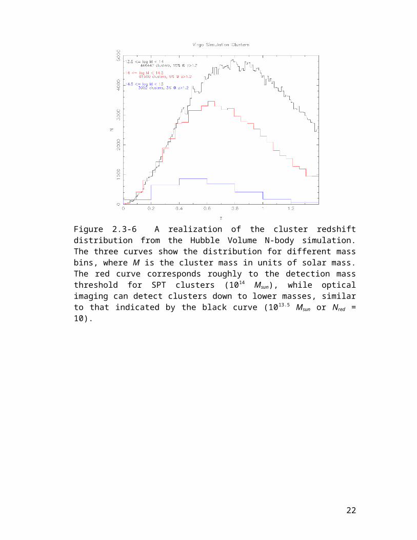
Figure 2.6-1. Projected constraints on M and w from the five-year DES SN survey. A flat cosmology has been assumed. Red: the SN survey alone; blue: joint constraints from SNe + 2dF (M = 0.278 ± 0.042) (left) and joint constraints from SNe and the SPT +DES cluster survey (right). Contours represent 1, 2, and 3 confidence levels. The curves at right represent the constraints on w after marginalization over M.

It is important to note that the DEC would be one of the primary instruments in the world for this type of supernova survey during its years of operation. We expect that the current generation of surveys will yield suggestive results and puzzles that will be addressed by the DEC SN work, so the baseline plan described above is very likely to be updated with a significantly more sophisticated plan that builds on what we know at the time we begin this effort. It is also significant that many of the challenges we face in the DEC SN survey, such as the lack of spectroscopic information on the majority of SNe, are the same as those which will be faced in the following decade when we attempt to use the incredible samples of SNe which the LSST will identify continuously throughout its operational lifetime. Just as the results of the current generation of SN surveys will guide us in updating and refining the strategies we will employ for the DEC SN survey, so will this survey provide crucial experience and guidance for deriving scientific results from the plethora of SNe discovered by LSST.

2.7 Photometric Redshifts

In order to achieve the dark energy scientific goals described above, the Dark Energy Survey will need to obtain accurate galaxy photometric redshifts to z ~ 1. This requirement is therefore a prime driver of the design and strategy of the Dark Energy Survey discussed in subsequent chapters. In the absence of spectroscopic data, redshifts of galaxies may be estimated using multi-band photometry, which may be thought of as very low-resolution spectroscopy. Though such photometric redshifts (or photo-z’s) are necessarily less accurate than true spectroscopic redshifts, they nonetheless are sufficient for the science applications we envision. Photo-z’s may be obtained more inexpensively and for much larger samples than is possible with spectroscopy.

There are two basic approaches to measuring galaxy photometric redshifts. The first relies on fitting model galaxy spectral energy distributions (SEDs) to the photometric data, where the models span a range of expected galaxy redshifts and spectral types (e.g., Sawicki et al. 1997). The second approach depends on using an existing spectroscopic

22

redshift sample as a training set to derive an empirical photometric redshift fitting relation (Connolly et al. 1995). There are advantages and disadvantages to each approach, as well as a number of variants and hybrids of these basic techniques (e.g., Csabai 2003). However, photometric redshift methods ultimately rely on measuring the signal in the photometric data arising from prominent “break” features present in galaxy spectra, e.g., the 4000Å break in red, early-type galaxies, or the Lyman break at 912Å in blue, star-forming galaxies. The key is to have photometric bands which cover such break features throughout the redshift range of interest, so that the primary redshift signal may be readily detected. Additional refinements in the photometric redshift measurement then come from the strength of the break features and the gross shape of the galaxy SED, as determined by the photometric data on either side of the spectral break.

2.7.1 Photometric Redshift Simulations for Cluster Galaxies

Cluster photometric redshift measurements are greatly facilitated by the strength of the 4000Å break feature prominently seen in the spectra of red cluster galaxies. This is illustrated in Figure 2.7-1, which shows a red, elliptical galaxy spectrum at redshifts 0, 0.5, and 1, superimposed on the griz filter bandpasses. The 4000Å break moves through the different filters as the galaxy redshift increases. Measurements of the relative galaxy fluxes through the different filters provide an estimate of the observed wavelength of the 4000Å break and hence of the galaxy redshift. This is demonstrated in Figure 2.7-2, where we compare photometric and spectroscopic redshifts for a sample of SDSS red galaxies, for which we are able to obtain photometric redshifts with a scatter z =0.03 out to redshifts z 0.6. However, at higher redshifts we do not have such large samples of red galaxies available, so we need to rely on Monte Carlo simulations to assess the quality of cluster galaxy photometric redshifts for the Dark Energy Survey.

Figure 2.7-1 The spectrum of a red, elliptical galaxy is shown at redshifts z =0, 0.5, and 1, with the location of the prominent 4000Å break feature marked. The spectra have been vertically offset for clarity. Also shown are the griz filter bandpasses, arbitrarily normalized to the same peak value. Photometric redshift information for red galaxies comes primarily from changes in the relative galaxy fluxes in the different filters as the 4000Å break moves to longer observed wavelengths at higher redshift.

23

In our Monte Carlo simulations, we adopt two different galaxy spectral energy distribution (SED) models to simulate the colors of a red cluster galaxy as a function of redshift: (1) an empirical non-evolving elliptical galaxy SED taken from the sample of Coleman, Wu, & Weedman (CWW; Coleman et al. 1980); and (2) a passively evolving elliptical galaxy model taken from the Pegase-2 SED library (Fioc & Rocca-Volmerange 1997). The Pegase-2 model is designed to match the colors of SDSS red galaxies at low redshifts, while the CWW model will provide an alternative SED for comparison purposes. Separate sets of Monte Carlo simulations are generated with galaxy absolute luminosities fixed at 0.5L*, L*, 2L*, or 5L*, where L* is the characteristic galaxy absolute luminosity (with 0.5L* being our faint luminosity limit of interest). 5000 galaxies are generated per simulation, distributed uniformly over redshifts 0<z<1. A flat cosmology, with and , is used to calculate galaxy apparent magnitudes as a function of redshift, and the models are normalized so that a 0.5L* galaxy at redshift one has a z-band magnitude of 23. The 10 galaxy magnitude limits for the Dark Energy Survey are griz = 24.6, 24.1, 24.0, 23.6. Expected galaxy photometric errors are calculated by appropriately scaling the S/N relative to the 10 magnitude limit, and by adding in quadrature a 2% error floor due to photometric calibration uncertainty. Photometric redshifts are determined using a polynomial-fitting technique (Connolly et al. 1995): we adopt a photometric redshift relation of the form redshift = f(g,r,i,z,g2,gr,r2,…), where f is a polynomial containing terms up to quadratic order in the griz magnitudes.

Figure 2.7-2 Photometric and spectroscopic redshifts are shown for a sample of SDSS red galaxies, for which a photometric redshift scatter z=0.03 is obtained.

Representative simulation results for 0.5L* and 2L* galaxies are shown in Figure 2.7-3, which plots the difference between photometric redshift and true input redshift as a function of the true redshift. We find good photometric redshift results for 0<z<1, with a 1 scatter z<0.03 per galaxy and only small systematic biases of size <0.01 in redshift. Note that we can do even better for a whole galaxy cluster, since we can average the photometric redshifts for, say, N individual cluster members and improve the photo-z estimate by the expected factor of .

24

One can see from Fig. 2.7-3 that there are small differences in the results for the CWW vs. Pegase-2 models, a consequence of the detailed differences in the color vs. redshift relations for the two galaxy models. In practice, for the Dark Energy Survey we will need to acquire a spectroscopic redshift training set (see below) in order to empirically measure the correct cluster galaxy SED to use for our final photo-z calibration, especially at redshifts z >0.7 where existing galaxy cluster data are very sparse.

2.7.2 Photometric Redshifts for the General Galaxy Population

We would also like to obtain photometric redshifts for the general galaxy population, beyond red cluster galaxies, in particular to facilitate dark energy constraints using weak lensing, galaxy clustering, and supernova measurements. Such photo-z’s are necessarily somewhat less accurate than those possible for cluster galaxies, as we must consider a much broader distribution of galaxy SEDs. Nonetheless, good photometric redshift measurements out to z 1 are still readily achieved for the general galaxy population.

Figure 2.7-3 Photometric redshift results for the 0.5L* and 2L* cluster galaxy Monte Carlo simulations. The red lines show the median difference between photometric and input redshift, the blue lines show the 1 scatter (68% limits), and the green dashed lines are set at z = 0.03.

25

We demonstrate this using the publicly available ground-based VRIz photometric data obtained by Capak et al. (2004) in the GOODS/HDF-N area, combined with a training set of 1800 spectroscopic redshifts from the compilations of Wirth et al. (2004) and Cowie et al. (2004). The VRIz photometry serves as a best-effort approximation to griz, as we are not aware of a sample with griz photometry of sufficient depth for this purpose. We add noise to the original VRIz photometry in order to match the Dark Energy Survey depths. We again derive photo-z’s using polynomial fitting, including terms up to quadratic order in the VRIz magnitudes, and the results are shown in Figure 2.7-4. We find a photometric redshift scatter z0.05 at i =22, increasing to z0.1 at i =24, the 10 galaxy limit for the Dark Energy Survey. The photo-z scatter increases at fainter magnitudes, as expected, and also increases with bluer galaxy color, a consequence of the weaker break features seen in the spectra of blue star-forming galaxies. Note that the photo-z trends vs. spectroscopic redshift are in general well behaved, except at the lowest redshifts, z<0.3, where the photometric redshift is scattered systematically high. This is likely a consequence of the lack of a constraining filter blueward of the 4000Å break at these low redshifts. In general, it will be important to understand any such biases by carefully measuring the photo-z error distribution using a large spectroscopic redshift training set. Two such large redshift surveys, the VIMOS VLT Deep Survey (VVDS; Le Fevre et al. 2003) and the Keck DEEP2 Survey (Davis et al. 2002), are both currently in progress. These surveys should provide spectroscopic redshifts sufficient to calibrate general galaxy population photo-z’s down to the Dark Energy Survey limit of i =24. In particular, the VVDS will obtain about 100,000 redshifts, and it is also being carried out from Chile. All the VVDS fields will be accessible to griz imaging using the Dark Energy Camera, enabling us to derive detailed photometric redshift calibrations for the Dark Energy Survey.

Figure 2.7-4 Photometric vs. spectroscopic redshifts for the general galaxy population in the GOODS/HDF-N field. Noise has been added to the original VRIz magnitudes in order to match the depths that will be reached by the Dark Energy Survey.

2.8 Appendix: Shear Sensitivity and Source Density for the Dark Energy Survey

For galaxy shape measurements, the deep i and z band exposures, which should also have the best seeing, will be the most useful. To be conservative, we consider only the 900

26

second i band exposures (in practice, the noise in shape estimates can be reduced by combining measurements in different bands). To estimate the shear sensitivity of the Survey, we studied a 900 sec CFH12K I band exposure taken in median seeing of 0.63'' (the CFHT mirror aperture is close to that of the Blanco 4m). We measured the ellipticities and sizes of the detected objects using an adaptive weighting scheme that is nearly optimal for lensing measurements (Bernstein and Jarvis 2002).

In estimating the shear, the ellipticity measurement of each source galaxy is relatively weighted by the inverse noise, which has contributions from shape noise (the intrinsic variance of galaxy shapes) and shape measurement error, an estimate of which is returned by the adaptive moments code for each object. In addition, the ellipticity of each galaxy is corrected for PSF dilution by a factor that depends on the square of the ratio of the galaxy size to the PSF—for small galaxies the correction is large, and uncertainty in the correction factor means these galaxies are further downweighted in the shear estimate. In the CFH12K image, the mean relative galaxy weight per magnitude bin is essentially unity out to IAB = 21.5 and drops to about 0.5 at , which is the nominal 10 magnitude limit for galaxies.

In the absence of measurement error and PSF dilution, the variance of the single component ellipticity for sources covering area A is given by . Including measurement error, PSF dilution, and the galaxy shear polarizability, we can write the rms as , where is the source galaxy density including noise weighting. This effective or weighted number density is convenient because it can be used with power spectrum noise estimates that assume the usual shape noise amplitude. The effective source density for the DES i band images is shown in the bottom panel of Fig.2.8-1 as a function of seeing. An increase in seeing has two effects: (i) the PSF is a larger fraction of the size of the faint source galaxies, so they receive less weight due to the larger PSF dilution factor; (ii) the effective number of CCD pixels per object is larger, increasing the sky background per object and therefore the shape measurement error. Fig.2.8-1 shows that for 0.9'' seeing, which should be typical for the DES, we expect an effective source galaxy density of about 10 arcmin. We have used this estimate in the analysis of the Dark Energy sensitivity above. The upper panel shows the shear sensitivity per component, which is just evaluated at degrees.

The survey depth also determines the redshift distribution of the source galaxies. In the estimates above, we used a median redshift . This is consistent with the distribution inferred from redshift surveys to , the expected depth of the DES, and with models of galaxy counts. The actual source redshift distribution for lensing will differ from that for a survey with this flux limit because (a) we include source galaxies beyond the 10detection limit, and (b) fainter galaxies contribute less weight. These correction effects go in opposite directions, and we expect the adopted median source redshift above to be reasonably accurate.

27

Figure 2.8-1 Upper panel: shear sensitivity for the Dark Energy Survey as a function of seeing, for 900 sec i band exposure. Lower panel: effective source galaxy density for lensing as function of seeing, for same exposure.

References

Annis, J., et al. 1999, AAS, 195, 1202Bahcall, N. A., et al. 2003, ApJS, 148, 243Battye, R. & Weller, J. 2003, PRD, 68, 083506 Bernstein, G., & Jarvis, M. 2002, AJ, 123, 583 Capak, P., et al. 2004, AJ, 127, 180 Coleman, G.D., Wu, C.-C., & Weedman, D.W. 1980, ApJS, 43, 393 (CWW) Connolly, A.J., et al. 1995, AJ, 110, 2655 Cooray, A., et al. 2001, ApJ, 557, L7Cowie, L.L., et al. 2004, AJ, submitted, astro-ph/0401354 Csabai, I., et al. 2003, AJ, 125, 580 Davis, M., et al. 2002, SPIE, astro-ph/0209419 Dodelson, S. 2003, astro-ph/0309277Dodelson, S., et al. 2002, ApJ, 572, 140Ellis, R.S., et al. 1997, ApJ, 483, 582Fioc, M., & Rocca-Volmerange, B. 1997, A&A, 326, 950 Gladders, M.D., et al. 2003, ApJ, 593, 48Gladders, M.D., & Yee, H.K.C. 2000, AJ, 120, 2148Haiman, Z. et al. 2001, ApJ, 553, 545Hamuy, M., et al. 1996a, AJ, 112, 2408Hamuy, M., et al. 1996b, AJ, 112, 2438Hu, W. 2003, PRD, 67, 1304Hu, W., et al. 1999, PRD, 59, 3512Hu, W., & Haiman, Z. 2003, PRD, 68, 3004Hu, W. & Jain, B. 2003, astro-ph/0312395Hu, W., & Kravtsov, A.V. 2003, ApJ, 584, 702Jenkins, A., et al. 2001, MNRAS, 321, 372Joffre, M. et al. 1999, in “Gravitational Lensing: Recent progress and Future Goals”, eds. T. Brainerd and C. Kochanek, ASP Conf. Series (2000)Kaiser, N. 1992, ApJ, 388, 272 Le Fevre, O., et al. 2003, astro-ph/0311475 Lidman, C. et al. 2003, A&A, in press, astro-ph/0310516Lima, M., & Hu, W. 2004, PRD, submitted, astro-ph/0401559Lin, Y.-T., et al. 2003, ApJ, 591, 749Lin, Y.-T., et al. 2004, ApJ, submitted, astro-ph/0402308Linder, E.V., & Jenkins, A. 2003, MNRAS, 346, 573Majumdar, S., & Mohr, J.J. 2003a, ApJ, 585, 603Majumdar, S., & Mohr, J.J. 2003b, ApJ, submitted, astro-ph/0305341McKay, T.A., et al. 2004, in preparationPerlmutter, S., et al. 1997, ApJ, 483, 565Perlmutter, S., et al. 1999, ApJ, 517, 565Perlmutter, S., & Schmidt, B.P. 2003, astro-ph/0303428 Riess, A., et al. 1998, AJ, 116, 1009Riess, A. G., Press, W. H., & Kirshner, R. P. 1996, ApJ, 473, 88

28

Sawicki, M.J., Lin, H., & Yee, H.K.C 1997, AJ, 113, 1 Sheldon, E.S., et al. 2001, ApJ, 554, 881Spergel, D.N., et al. 2003, ApJS, 148, 195Stanford, S.A., et al. 1998, ApJ, 492, 461Tegmark, M., et al. 2002, ApJ, 571, 191Tegmark, M., et al. 2003, PRD, in press, astro-ph/0310723van Dokkum, P.G., et al. 2000, ApJ, 541, 95van Dokkum, P.G., et al. 2001, ApJ, 552, L101Wang, L., & Steinhardt, P.J. 1998, ApJ, 508, 483Wirth, G.D., et al. 2004, AJ, submitted, astro-ph/040135

29

3. Survey Strategy

3.1 Introduction

The goals of our survey require a large area map of 5000 square degrees of sky to i=24 in 4 bandpasses, with photometric calibration sufficient for precise photometric redshifts for all galaxies, implying photometric calibration accuracy of around 2%. This chapter describes the Dark Energy Survey and provides a proposal for the imaging strategy and photometric calibration. We intend to continue to optimize these strategies.

We first summarize the science goals described in Chapter 2, and follow that with a section laying out the decisions and calculations that lead to many of the technical specifications. We then describe tilings as a way to think about collecting the survey data, and use tilings in a photometric calibration strategy designed to achieve the calibration accuracies the survey needs. At the end of the chapter, we give the expanded technical specifications that flow from the consideration of the science program as a survey project.

3.2 Science Goals

The dark energy probes we outline in Chapter 2 constrain dark energy using a four-fold approach of cluster abundances, weak lensing shear, galaxy power spectrum, and supernovae. These science goals may be summarized as follows:

5000 square degrees in the South Galactic Cap, overlapping SPT and redshift survey areas.

Photometric redshifts to z=1.0 and ½ L* with δz <= 0.05, using SDSS g, r, i, z. This implies a 2% photometric calibration.

PSF sufficient for weak lensing, FWHM <= 0.9”.

We will develop these science goals into technical requirements in the following sections.

3.3 Science Goals to Survey Specifications

3.3.1 Survey Footprint

We plan to image 5000 square degrees in the following areas:

The South Galactic Cap: The primary decision that shapes the footprint is overlap with the South Pole Telescope survey area, 4000 square degrees area bounded by Dec ≤ -30° and 20hr ≤ RA ≤ 6hr. The south celestial pole, overhead of the South Pole, is an area of high galactic dust and thus has higher uncertainty on magnitudes and colors, and for the SPT is an area of higher foreground. We will excise this area from the survey. The primary survey area spans –30˚ declination to –75˚ declination, extends from 20hr to 6hr, and covers the bulk of the low extinction area available.

The 700 square degrees area: We select a region that connects the main survey

area with the photometric redshift area. This region is optimally placed for providing targets and optical follow up for the large optical telescopes and radio telescopes in Chile.

30

The equatorial stripe: The 200 square degrees region on the equator covers existing redshift surveys from the SDSS and VLT. Data on these areas are needed to calibrate the photometric redshifts. We will need on the order of 1000 redshifts per 0.1 bin in z to calibrate the photometric redshifts, so we must image areas already under study in large redshift surveys. The equator between 21h and 6 hr contains the SDSS Southern Survey, 100,000 redshifts of a variety of galaxy and stellar samples, probing higher redshifts, fainter magnitudes, and smaller objects than the main SDSS survey. This area also contains 8 square degrees of the VIMOS-VLT Survey Wide (down to magnitude IAB = 22.5) and 2 square degrees of the VIMOS-VLT Survey Deep (down to magnitude IAB = 24.5).

Figure 3.1. Map of the galactic dust in the South Galactic Cap. Our reference design survey footprint is inside the green line. The Large Magellanic Cloud is visible in the corner of the survey area.

3.3.2 Limiting Magnitudes

Our science goals demand that we reach the magnitude of a 0.5L* galaxy at z=1.0, where L* is a luminosity characteristic of the galaxy population. From Blanton et al (2003) we find that a * galaxy has an i-band absolute magnitude (coverted to redshift 0 and evolution corrected). Using a passively evolving old stellar population model appropriate for high luminosity cluster galaxies, we find that this corresponds at redshift one to z band magnitude z=23.3. We will be requiring 10 observations, as needed by our optical cluster finding and photometric redshift techniques. Our existing test data show that 10is near where the number counts turn over, an indication that it is close to the completeness limit. We will want to go somewhat deeper, say 0.3 magnitudes, in order to safely construct a flux-limited sample of galaxies. We therefore require a limiting magnitude in the z band of z=23.6.

31

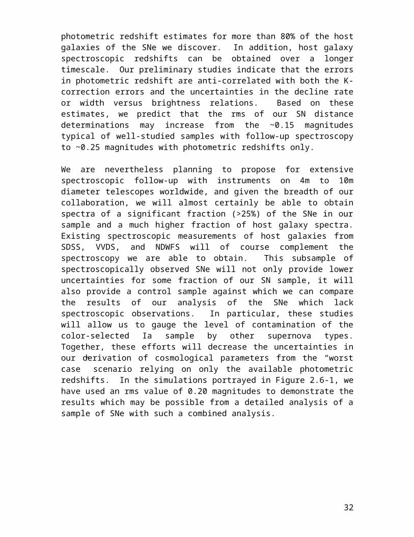
We need precise colors on the cluster galaxies in order to calculate photometric redshifts. We already know the limiting z magnitude, so we must calculate the g, r, i magnitudes. The magnitude required is the magnitude of the galaxy at the redshift where the 4000Å break leaves the blue filter and enters the redder filter. This happens at redshifts of 0.35,0.65,1.0 for the SDSS filters g, r, i. Using the same passively evolving model, we find that these redshifts correspond to magnitudes g, r, i = 22.8, 23.4, 24.0.

Table 3.1Filter g r i zLimiting magnitude (10) 22.8 23.4 24.0 23.6CCD QE 0.65 0.85 0.65 0.5Filter and optics T dλ / λ 0.18 0.14 0.13 0.18Sky brightness (mag/sq-arcsec) 21.7 20.7 20.0 18.7Sky Brightness 45o from moon 19.7 19.7 19.25 18.5Minimum integration times (sec) 27 130 900 1600

3.3.3 Integration Times

The integration time is the total of all individual exposures.

We will need to calculate the exposure times to reach a signal to noise of 10 at the limiting magnitudes. The calculation of the exposure time depends on the mirror area, the throughput of the system, the read noise of the instrument, the pixel size, the sky background, and the area over which the object is spread.

The Blanco 4m telescope has a light collecting area of 10.0 sq-meter. We will use the SDSS filters, but our reference design has two more optical elements than the SDSS design. In Table 3.1 we give CCD quantum efficiencies (QE) and the transmission of the optics and filters (T dλ / λ) using those from the SDSS, except that we assume (1) a x5 better QE in z as we are using high red response full depletion CCDs, (2) a wider z filter, and (3) an additional overall transmission factor of 0.9, modeling the losses in transmission due to the extra two elements. We assume the camera has a read noise of , and that the pixel size is 0.27”/pixel.

The SDSS has measured the sky brightness in each of the filters, albeit at a site distant from CTIO, and we tabulate it in Table 3.1. The sky brightness varies in time. A half magnitude increase in the sky brightness results in a quarter magnitude decrease in the limiting magnitude. The solar cycle causes sky brightness variations on the order of 0.5 magnitudes, and the next solar max is roughly 2012, we note that the sky brightnesses in Table 3.1 are from SDSS data taken in the years near the last solar maximum. Table 3.1 also shows the effect of observing near a full moon (to be precise, within 45 degrees of a moon at a phase fuller than half), using data from the SDSS Photometric Telescope. This line shows that we can image through the i and z filters in such conditions, so called grey time.

The sky brightness contributes to the noise in galaxy magnitudes and colors in proportion

32

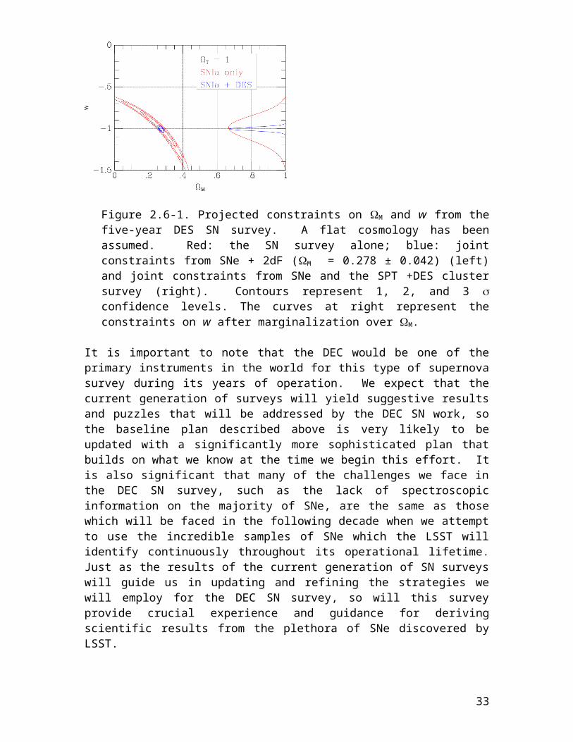
to the area of the aperture one uses to measure the magnitudes. We assume the seeing at the Blanco 4m is 1.0”, and use an aperture of 1.7” diameter, as is appropriate for the measurement of the colors of faint galaxies, to measure the magnitude.

The result is the exposure times listed in Table 3.1.

3.3.4 Available Time and Weather

We assume our survey will use 30% of the time available over a five year period. We have estimated the number of useful hours available for the survey in the five year period 2008-2012 via an analysis that includes the observing impact of weather and the astronomy of the lunar cycle. The details of this calculation are presented in Wester (2004) and are summarized below.

Astronomy- We define dark time as the hours between the evening and morning 18-degree astronomical twilight when no moon is above the horizon. Grey time is defined similarly but allows for the presence of the moon and 18- to 12-degree twilight. We assume a survey that includes a total of 143 nights (5 lunar cycles) that end in January prior to the first night during which there is no dark time because the moon is always above the horizon. This survey starts on different dates in different survey years in 2008-2012 due to the lunar cycle, which impacts the available time since the time between astronomical twilight varies over the course of a year.

Weather- To estimate the impact of weather, we analyze data made available by CTIO that quantifies the measured cloud cover during four quarters of each night from 1975-2003. We count only photometric time, defined to be when there is no cloud cover. While we have calculated the average fraction of cloudless nights as a function of day of the year, we have also performed a more sophisticated analysis that maps the historical weather statistics in all five-year periods from 1975-2003 onto our planned observing time in 2008-2012. In this way, we have studied the effects of extreme conditions (such as El Nino years) as well as the effect of averaging over a five-year period. We find average values of 1749 dark and 2142 grey hours. See Figure 3.2, where the average time, both dark and gray, is plotted as a dashed line.

We will not have the entire 5 lunations available to us. We multiply the 5 lunation total by 0.75 to model the time allocated to us by NOAO. We thus obtain 1300 hours of useful dark time and 1600 hours of useful grey time and an estimate of 2900 hours of photometric time over the survey.

Our calculation of survey time includes only photometric time. There is another 950 hours available with non-photometric, but not overcast, conditions. Some data taken during this time will be usable, if of lower quality.

33

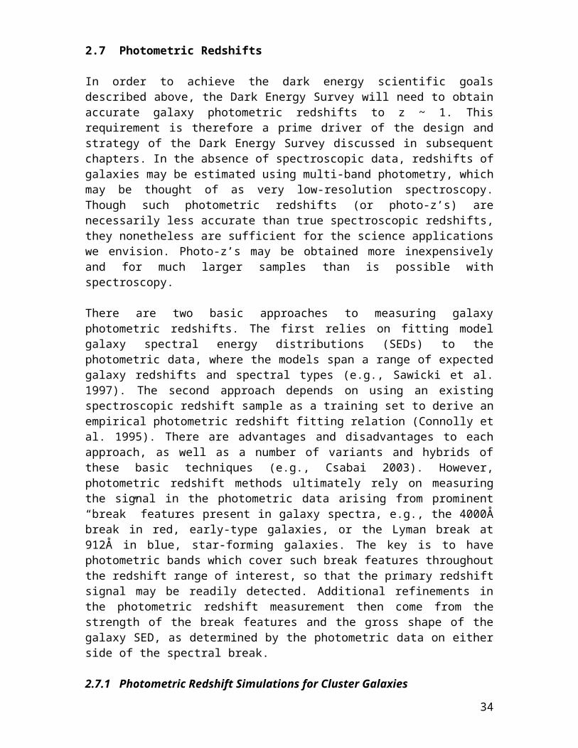
Figure 3.2 The total cloudless time over a 5-lunation period ending in January at CTIO, over the last 30 years.

3.3.5 Camera Size

We start from the observation that a 2.1o field of view corrector is technically feasible on our timescale, and that the area of an inscribed hexagon is 2.9 square degrees. We will show that a camera of these dimensions is sufficient for our science goals.

For the purposes of the following calculation, it is convenient to think of the data as making up a field as being taken at one time. We define a field to be all observations taken through all bandpasses on a given location on the sky. The total exposure time is taken to be 3500 seconds per field, as given in Table 3.3

The overhead is estimated in two parts, slewing and everything else. The slew time of the Blanco Telescope is 35 seconds for slews less than 4 degrees, greater than both the predicted CCD readout time (18 seconds in Chapter 4) and the predicted filter change time (20 seconds in Chapter 4). We assume that the total integration time is broken into 5 or more shorter exposures of at least 100 seconds (see the photometric calibration section later in this chapter). We assume that the telescope is moved after every exposure. We note that the overhead may be reduced by increasing the individual exposure time for data taken in filters i and z, and maybe somewhat reduced by taking data in two filters before a slew. The total number of images over all bandpasses is 35, leading to 35 slews and a total of 1200 seconds of overhead per field attributable to slewing. We take nightly

34

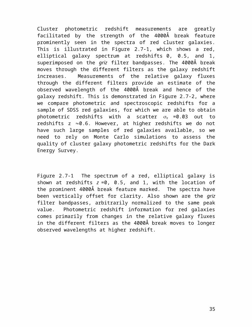
setup time as 0.5 hour, and we assume 4 observations of standard stars per night that take a total of 0.5 hour. We then assume that equipment failure over the life of the survey averages to 0.5 hour per night. Taking this overhead per night of 1.5 hours, dividing by 6 fields per night (the survey average is a 9.5 hour night and 1.5 hours is taken up), we find 900 seconds of overhead to add to the slew times. The total overhead is 2100 seconds. The grand total time spent per field is then 5600 seconds. These numbers are summarized in Table 3.2.

Table 3.2Filter: g, r, i, zTotal integration time: 500, 500, 900, 1600 secondsNumber of exposures: 5, 5, 9, 16Total integration per field: 3500Pointing overhead: 35 seconds slew, 35 images: 1200 seconds.Other overhead per field: 900 secondsTotal per field: 5600 seconds

We have 2900 hours available to us, and we plan to devote 10% of the time to supernova observations, leaving 2600 hours for the survey. Observing 5000 deg2 over 2600 hours implies an observing rate of 1.9 deg2/hr. The time spent on each field is 5600 seconds (1.55 hrs), so the camera area needed is then

Area = 1.9 deg2/hr * 1.55 hrs/field = 3.0 deg2

Note that a corrector with a 2.1 degree diameter field of view has an area of 3.5 square degrees. The largest useful pattern for tiling the sky is a hexagon, which if inscribed in 2.1 degree diameter circle has an area of 2.9 sq-degrees. The current CCD layout in Chapter 4 has a tiling area of 3.0 sq-degrees with a 5% non-active area. We see that our current camera design is sufficient to perform a 5000 deg2 in the time allotted to us.

Note that we only included photometric time in this calculation. At CTIO, the majority of time during our observing season is photometric, still we estimate in section 3.3.4 that 950 hours of usable non-photometric time is available and some of it will be useful for survey data.

3.3.6 Seeing

Both the site seeing and the weather statistics suggest that the best seeing is Oct. to Jan. and we hope to observe during that time. The FWHM of a star image scales with wavelength and airmass as:

where z is the zenith angle, λ is the wavelength and sec(z) is approximately the airmass. For the same airmass, 0.9” seeing in r band corresponds to 0.8” in z band, and seeing of 0.8” become 0.9” when the airmass changes from 1 to 1.2.

In order to attain this seeing, the camera must be kept in focus and the telescope tracking the stars. We calculate that in 1 second scale exposures we will have 10 measurements of stars down to i band magnitudes i~18.5. We estimate the stellar density at these magnitudes to be 0.2 stars/sq-arcmin. We find that we need 25-50 arcmin2 of guider area to have a low likelihood of not finding a star to guide on over the course of the survey.

35

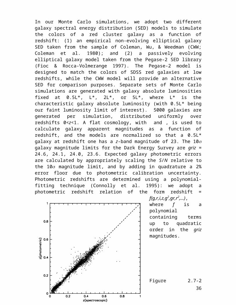
For focusing, we will use survey length exposures, but we need ~100 S/N measurements of stars. The magnitude range of interest is roughly the same as for guiding, so the stellar density is roughly the same. 3.4 Tiling Strategy

Tilings are unique, non-overlapping coverings of an area. Hexagons can tile the plane, whereas circles either overlap or leave gaps. Hexagons provide the optimal tiling of the plane, a 2d space filling pattern that has the maximum area for its longest cross section. An actual focal plane layout of CCDs may only approximate a hexagon; what is then important is the area of the tile in the tiling.

There are optimal mapping strategies for hexagon maps in the sense of maximizing unique interlocking overlaps for photometric calibration purposes. Arbitrarily take the first tiling as the reference tiling. The second and third tilings have hex centers placed on the vertices of the reference tiling such that the three centers form one of the 6 triangles that make up a hexagon (Figure 3.3a). They provide 33% overlaps with 3 hexagons from the reference tiling. The 4th through 6th tilings have hex centers placed on the centers of the edges of the reference tiling (Figure 3.3b). These provide 42% overlaps with 2 reference tiling hexes, and 8% overlaps with two others. This set of 6 tilings provides the maximally unique interlocking pattern. Diminishing returns enter after 6 tilings, and one may either repeat the sequence or dither.

Figure 3.3. a) The left panel shows the reference tiling in black, and the two 33% overlap tilings in red and blue. b) The right panel shows the reference tiling and the three 42% overlap tilings in purple, green, and gold. These six tilings provide a maximally unique interlocking tiling pattern.

There are about 1667 tiles in our 5000 square degrees survey given the 3.0 square degrees camera layout in Chapter 4. We currently estimate between 25 and 35 tiling of the area. 3.5 Photometric Calibrations

3.5.1 Photometry of Large Area Surveys

We are proposing a large area, multicolor, imaging survey that requires precision photometry. Traditional photometric reduction which places observations onto a standard system are inappropriate for extremely large sets of homogeneous photometric data produced using a single instrument. It is much more important for these surveys to be internally consistent than it is for them to be on previously established photometric

36

systems. For extremely large surveys, the aim of calibration is to produce data sets for which:

The magnitudes may be calculated by convolving a spectrum with good spectrophotometry with the system bandpasses, and

The magnitudes vary only by 2.5log10(), where are the ratio of the photon fluxes, independent of position.

The first goal puts a premium on knowing the system response curve with precision. The second goal demands knowing the atmospheric effects, but also puts a premium on understanding flat fielding and scattered light effects.

3.5.2 Determining the System Response

Understanding the system response curves is critical to using photometric redshifts, and is in fact fundamental to understanding the photometric data. System response curves are relative efficiency curves over the entire wavelength coverage of the instrument. Ideally one would include the primary mirror, but in practice the reflectivity curve of aluminum is well known and flat vs. wavelength. We plan to measure response curves that include the effects of the correctors, filters, and the CCD quantum efficiency. Convolutions of spectral energy distributions with the system response curves are best done with at least 100 resolution elements across the bandpass. For our ~150 nm wide filters, we need about 1.5 nm resolution. Detailed calibration is done once a season for every CCD. We are investigating several options for this purpose, including one more optimized for supernova operations.

3.5.3 The Photometric Calibration

The equation for photometry is m = -2.5 logC - a- k(t)X - cMX

where m is the magnitude of an object, C is the measured counts, a is the measured zeropoint, k(t) is the time dependent extinction coefficient, X is the airmass, c is the second-order extinction coefficient. The last term reflects the varying extinction across the broad filters typical of large area surveys. The aim is to reduce the complexity of this equation.

Ignore second order extinction: Wide area surveys usually obtain observations at low to moderate airmasses. The SDSS maximum airmass limit was 1.5, and the median airmass was about 1.3. The values of c are of order 0.03, so the second-order extinction term is of order 0.005. Ignoring it places a photometry calibration error floor somewhat below 1%.

Absorb k(t)X into the zeropoint: The zeropoint a changes randomly night to night, while the extinction coefficient k(t) changes randomly both night to night and drifts during a night. If one were to arrange to observe only at one airmass during the night, the equation would become:

m = -2.5 logC - a(t)All-sky photometry as routinely practiced is suboptimal for a pointed survey that covers a large fraction of the sky multiple times, as it spends far too much time deriving separate

37

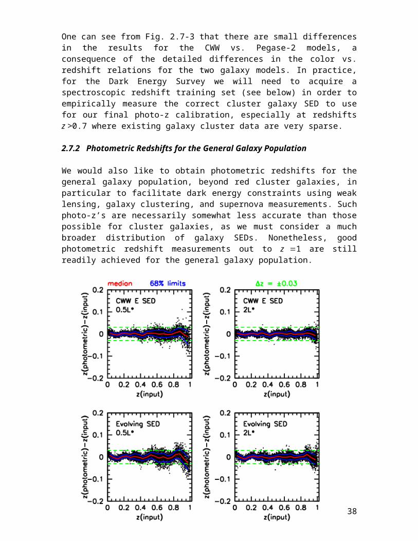
zeropoints and extinction coefficients. With the large amounts of data taken at a single airmass, as anticipated for our survey, the equations and photometric calibration become more straightforward.3.5.4 Photometric Calibration Through Mapping Strategies

Techniques developed for CMB mapping strategies (Wright 19962, Tegmark 19973) can be applied to the problem of developing photometric calibrations across the survey area. The mapping strategies are in essence least squares solutions to the problem of estimating the underlying map given many noisy observations. One forms linear equations of the form y=Ax+n, where y is the data, n the noise, A is the known observation matrix and x is the underlying map one is solving for. One solves for the map x =Wy, by constructing W via This method is fast, simple, and minimizes the error map variance in the case of white noise.

The maximally overlapping tilings make this a powerful technique, and we can use them in at least two ways:

Absolute photometry, where one uses standard stars to tie hexes together.

Relative photometry, where one uses the ratios of the fluxes of the same stars observed on two different images to tie the photometry together.

The first, the absolute photometry strategy, would follow from our reference design observing plan, where we observe constant airmass tracks and observe a standard star afterwards. We would then have about 4 standard stars a night, which translates to roughly 5% all sky photometry for the night. Assigning the calculated zeropoints to each hex, one uses the multiple observations of the hexes in a least squares fit, involving all hexes observed, to reduce the scatter in the zeropoints across the final tiling. Our simulation suggests one gets a reduction of the scatter in the zeropoints, where N is the number of tilings in a given filter.

The second strategy is even more powerful, because of the precision of relative photometry. It is clear that one knows the relative flux between overlapping images much better than one knows the zeropoints of the images. The numerical precision of relative photometry is much better than 1%, when one is talking about stars appearing in two different images. What limits this approach is systematic errors, primarily flat fielding and scattered light. Both of these are more likely to be more problematic at the edges of a camera that fills a focal plane. The overlapping hex tilings allow one to average these out. The relative photometry strategy produces a map which is very flat, and in that sense has very good relative magnitudes. The zeropoint itself is unknown. We would either have to use the absolute photometry strategy in some fashion to calibrate this map, or to use perhaps 100 stars of known magnitudes in the map to provide the absolute calibration. The likely saturation point of the CCDs will be roughly i band magnitude i=17.5, and the likely point of onset of non-linear behavior in the CCD amplifiers a factor of 2 lower, at roughly i band magnitude i=18. This means that we will not be able to use the SDSS standard stars of Tucker, Smith, and collaborators directly, and will have to explore the options more thoroughly.

38

3.5.6 Quality Assurance: Checking the Photometry

The mapping strategies we have explored aim to measure magnitudes, and make no use of colors. This allows us to use known astrophysics to check our photometry. The stellar locus in color-color space has extremely well defined principal axes. The SDSS has shown that in the twin color spaces of g-r, r-i and r-i, i-z one knows the location and direction of the principal axes to a precision of

where is of order 0.003 magnitudes. In single exposures of 100s, the DEC reaches about 21 mag at a S/N=100. This implies about 2000 stars/sq-degree. The SDSS experience is that only about 1/4 of these are clean, in the sense of being located away from image edges and not blended with other objects. We’ll have about 500/sq-degree of useful stars, which corresponds to roughly 20/CCD. This means we can use the stellar locus in three ways to check our calibrations:

CCD calibration on full sensor scales: Three adjacent hexes provide enough stars to check the calibration on each CCD to 0.003. Recall that the equation above scales to 64 bins, and our current designs have 60 CCDs.

CCD calibration in 100x100 pixel scales: A complete tiling of 2000 hexes provides enough stars that when one selects all the stars observed by a given CCD one has enough statistics to explore the calibration in 100x100 pixel sub-regions.

CCD calibration on 300x300 pixel scales: Breaking the complete tiling up into 10 blocks of 200 hexes each, one can do the same on 300x300 pixel sub-regions and check for variations with, say, right ascension.

It is worth pointing out how powerful this check is. We are calibrating the magnitudes independently of the colors, and checking the resulting colors, which are magnitude differences using a precise test.

3.6 Survey Simulations

We are developing simulations to help us understand the survey in operation.

3.6.1 Observing Strategies

If one observes at a single airmass, one obtains data with great power to perform cross checks on zeropoints. We developed a survey simulation and used it to model a survey consisting entirely of constant airmass tracks.

The simulation consists of the celestial timings, the survey area, and a simple weather model. It was used to explore whether one can in fact observe a large sky area efficiently by following constant airmass tracks. Applying a simple set of rules for the observing strategy, such as "find closest hex at predefined airmass", with a set of stopping conditions, such as "no unobserved hex with that airmass available", leads to data taken

39

along paths as shown in Figure 3.4. This observing strategy leads to stripes of a wide variety of lengths and trajectories across the region, naturally connecting neighboring tiles on observations from different nights, and to a low median airmass of 1.2.

Figure 3.4. This shows the paths of the constant airmass observation stripes for one tiling. Clearly there will be many interconnections across tilings.

3.6.2 Absolute Calibration Strategies

We extended the survey simulation we developed above to include a model for the atmosphere that had, among other effects, a time varying extinction coefficient on each night. We solved for the zeropoint map using the coadd technique described above. We find that one determines the zeropoint of the coadded images with precision, where N is the number of tilings in that filter. Starting at 5% rms zeropoint error, one reaches 2% after 5 years by leveraging the many observations of standards that are taken. This 2% is the RMS constraint on any gradients or small scale features in the map. We show a map of photometry errors resulting from this approach in Figure 3.5.

Figure 3.5 This figure shows maps of the photometric calibration error. The left panel shows the map resulting after 5 years using the absolute calibration strategy. The rms scatter in this map is =0.037, starting with photometry good to =0.10. The panel on the right shows the map resulting after 3 years using the relative photometry approach. The rms scatter in this map is =0.013, starting with photometry good to =0.1, and with systematics imbedded at the =0.03 level. The bar at the bottom shows the lookup table for errors of -0.20 to +0.20, a 2 range on the input rms scatter

40

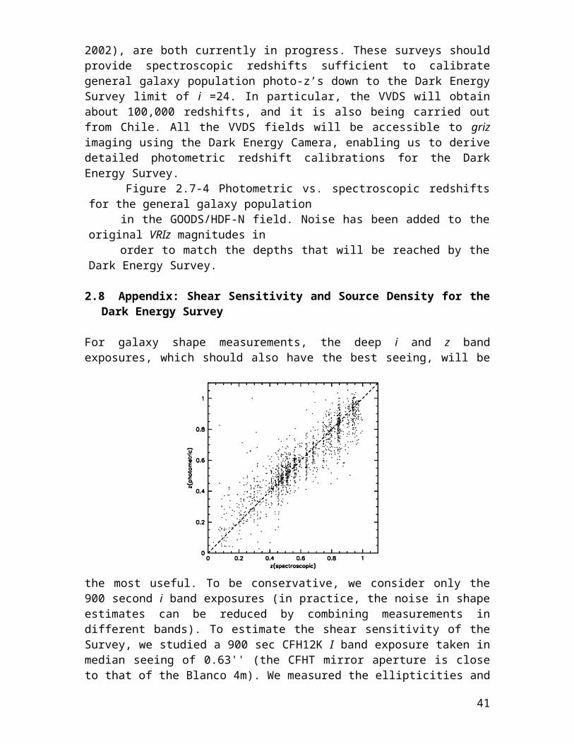
3.6.3 Relative calibration strategies

We further extended the survey simulation to include small and large scale flat fielding errors and small and large-scale scattered light errors, all on the scale of 2%. We solved for the relative photometry map using the coadd technique described above. For one tiling observation the resulting map is flat to =0.034, for two tilings the map has =0.018, and a five tiling map has =0.010. An image of the resulting map is shown in Figure 3.5. There is clearly great promise in this approach.

3.7 Resources for Survey Operations

The Survey Strategy team will operate as a working group with Annis as lead and Lin as deputy with contributions from Flaugher, Frieman, Mohr, Tucker, Wester. There will be the need for an algorithmic computing professional to help with the development and production of the simulations.

This group will continue the development of the survey simulation. This has several parts.

The observing model will have to be developed with an eye towards maximizing efficiency.

The photometric calibration strategies will need to be extended, especially to incorporate improved models for the atmosphere and the instrument.

Catalog level simulations will extend these simulations all the way to the data stream. We have a start with Wechsler’s catalog level simulations of the galaxies and clusters we expect out to z=1.2.

Image simulations that incorporate more sophisticated models of the instrument and of the astrophysics will be valuable. We have a start on this with Lin and Sheldon’s image simulation. The image simulation effort will provide the data for the mock data challenge (described in Chapter 5), where we send a large amount of simulated survey data through the reduction stream as a test of the system.

We aim to understand and characterize the camera as an astronomical photometry system. This requires that we develop a model of the camera containing:

CCD characteristics System response Flat fields Scattered and stray light Optics

These effects will be included in the simulations. The information required for the camera model will come from various sources. The CCD characteristics measured by the CCD development group. The measurement of the system response, will require designing and implementing hardware work with the completed camera. The scattered and stray light analysis, will be contracted, and the results of their analyses incorporated into the simulations.

41

3.8 Summary

The dark energy probes outlined in Chapter 2, require a survey whose science goals may be summarized as follows:

5000 square degrees in the South Galactic Cap, overlapping SPT and redshift survey areas.

Photometric redshifts to z=1.0 and ½ L* with δz <= 0.05, using SDSS g, r, i, z. This implies a 2% photometric calibration.

PSF sufficient for weak lensing, FWHM <= 0.9”.

The analysis of this chapter developed these goals into a survey specification, which may be summarized as:

1. 5000 square degrees in the South Galactic Capa. 4000 square degrees to overlap the SPT survey area b. 270 square degrees of overlap with redshift surveys for photo-z training

samplesc. 700 square degrees optimal for CTIO and Atacama telescopes

2. Photometric redshifts to z=1.1 and ½ L* with δz <= 0.05.a. SDSS g, r, i, z are sufficient, if z is made 5x more sensitiveb. g=24.6.1 r= 24.1, i=24.0 z=23.6c. photometric calibration to 2%d. at least 5 exposures per filter

3. PSF and galaxy density sufficient for weak lensinga. Seeing <= 0.9”b. Pixel size to fully resolve PSFc. Focus and guiding sufficient to obtain 0.9”

The technical specifications that follow from this analysis:1. A survey instrument with sufficient grasp

a. optics with a 2.1 degree diameter field of viewb. a focal plane array with a tiling pattern size of 3 square degreesc. quantum efficiency in the z band of ≥ 50%.

For completeness, we show the limiting magnitudes that result from these survey specifications. We go deeper than required in g and r in order to achieve the photometric calibration requirement of having 5 or more exposures per filter.

Table 3.3Magnitude and Exposure TimesFilter g r i zExposure 500 500 900 1600mag (10) 24.6 24.1 24.0 23.6

42

References

1 Wester, W. (2004), DECam note, “Useful Observation Time at CTIO for the Dark Energy Camera Survey”

2 Wright, E.L. (1996), astro-ph/96120063 Tegmark, M. (1997), ApJ, 480, L87

43

4. The Dark Energy Survey Instrument

4.1 The Reference Design

This section describes the essential elements of the Reference Design for the Dark Energy Survey Instrument. It includes the camera, cooling, wide-field optical system, the data acquisition system (DAQ), and the mechanical and electrical interfaces to the Blanco telescope and its infrastructure. The Reference Design is not intended to be the final design, since we are still evaluating a number of technical choices. Nevertheless, it has allowed us develop a reasonably complete enumeration of the tasks that must be executed in order to build the Dark Energy Survey Instrument. In Section 4.2, we describe the present configuration of the Blanco and in sections 4.3-4.8, we give the reasoning behind the choices we made in the Reference Design and the issues that we must resolve before proceeding to a final design. With the reference design in mind, we have developed a preliminary Work Breakdown Structure (WBS) and identified the critical items that will require development before production can start. We have made a very preliminary estimate of the schedule and the resources that will be needed for the construction of the instrument and its interfaces to the Blanco as well as the commissioning of the instrument in Cerro Tololo. This is provided in section 4.9 along with a brief outline of our R&D plans for the near term. These initial estimates suggest that we should be able to deliver a fully tested instrument with a fully integrated and tested DAQ to CTIO in Jan. 2008.

4.2 The Blanco Telescope

The Blanco is an equatorial mount telescope with a flip cage at the prime focus. A photograph of the Mayall telescope at Kitt Peak, which is a near twin of the Blanco, is shown in Figure 4.1 and a drawing of the layout of the optical components in the Blanco cage is shown in Figure 4.2. Together, they provide a perspective of the layout of components at the Blanco prime focus.

In the present configuration on the Blanco, the light from the primary mirror is focused onto Mosaic II, the existing wide-field imaging camera, when the cage is in the position shown in Figures 4.1 and 4.2. Mosaic II consists of eight 2K x 4K CCDs. An optical system corrects the field of view over an angular diameter of 0.85 degrees. It consists of 4 lenses and an atmospheric dispersion corrector. The optical system, filters, camera and the f/8 secondary mirror are all mounted on the cage that is attached by the spider to a ring. When the cage is flipped through an angle of 180 degrees into the other position, the f/8 secondary mirror reflects the primary beam on to the Cassegrain focus. The prime focus plate scale at the Blanco is 55 microns/arcsec (1 meter/5 degrees). Table 4.1 provides a further enumeration of some of the essential parameters of the Blanco telescope.

44

Figure 4.1 Side view of the cage on the Mayall telescope. The Mosaic camera and corrector are mounted inside the cage. The spider attaches the barrel to a ring that is in turn attached to the main truss (white) of the telescope. The ring can flip the orientation of the cage such that the other end points toward the primary.

Figure 4.2 The cage and optical components of the Blanco 4m telescope. The corrector lenses are contained in a barrel, which is supported by a pedestal bolted to the centerpiece of the cage. The secondary mirror is located on the far left.

45

Cage

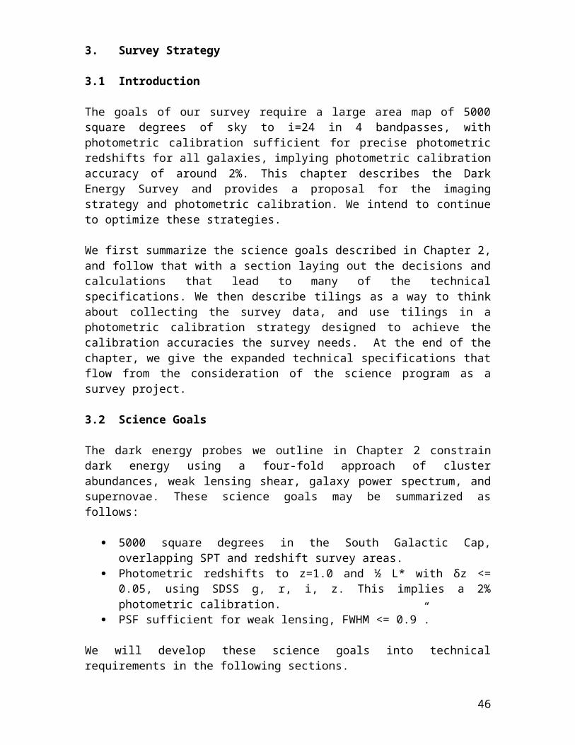
Table 4.1 Parameters of the Blanco Telescope and Facilities at the Site

Blanco location Lat. 30o 10’ S,Long. 70 o 49’ WAltitude 2200 m (7200 ft)

Primary Mirror 4m dia., 50cm thick, 15 tonTelescope Mount EquatorialPrime Focus f/2.87Plate scale 55 microns/arcsecSeeing FWHM 0.8 to 1.1 arcsecDome Temp. Range -10 to +25 deg. CSlew time 35 sec. for 1 or 2 deg. SlewsGuider Update Rate 2 sec.Adj. Range needed for focus ~2cmN2 plant on mountain top 9 lts/hr capacity,

50,000 lts annual consumptionCost ~ $1/lt

Power 120V, 60hz in Dome and Cage

We propose to replace the cage and everything inside it except for the atmospheric dispersion corrector which is not needed for our survey due to the proposed short exposure times. We also propose to replace the mechanical, electrical, and communication interfaces between the cage and telescope. The f/8 secondary mirror will no longer be permanently attached to the cage. Instead a precision mounting system that will be permanently attached to the cage will allow the mirror to be reinstalled during the day to the required alignment tolerances.

The Mosaic II has two guide cameras in addition to the eight image CCDs. The guide cameras provide small corrections for the telescope tracking system so that a star image will stay in precisely the same location during an exposure. In our reference design we have CCDs on the focal plane devoted to guiding, along with additional CCDs devoted to a new semi-automatic focusing system.

4.3 Technical Specification

Our survey goals and the survey strategy were presented in Chapters 2 and 3. When combined with the performance parameters of the Blanco Telescope, the site conditions and infrastructure our science goals determine the technical specifications of our proposed instrument. A brief summary of those specifications is as follows:

A 2.1 degree field of view corrector, and a focal plane in which >~80% of the field of view is active.

Four filters with appropriate bandpasses to determine the redshifts of red galaxies by their colors to a typical precision of 0.02 in redshift over a redshift range from 0.1 to 1.

46

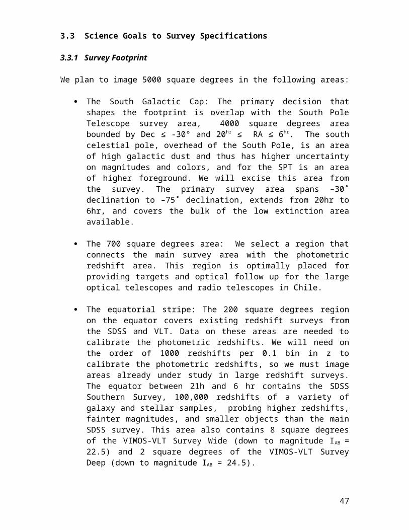
CCDs with a QE in the z band of >~50% to reach the magnitude limits of 24.0 in the i band and 23.6 in the z band.

A pixel size that allows sufficient sampling to permit precision photometry.

Guide and focus systems with interfaces to the Blanco telescope drive motors.

A system capable of providing sufficient Liquid Nitrogen (LN2) to cool the CCDs.

Table 3.2: The median seeing at the Cerro Tololo site.

4.4 General Layout of the Reference DesignTable 3.2: The median seeing at the Cerro Tololo site.

The Reference Design has six distinct subprojects. These are:

1) the primary cage and integration with all cryogenic, electrical, and mechanical systems

2) the optical system3) the CCDs, CCD packaging and front-end electronics inside the camera vessel 4) the camera vessel and cooling system, including the mechanical support for the

CCDs5) the data acquisition system

These will be discussed in detail in the next sections; this section gives a brief overview

47

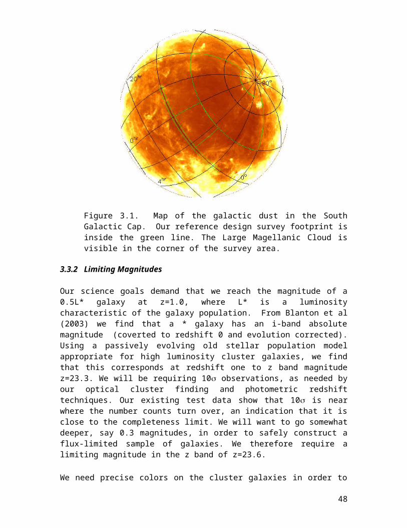
of the layout.

Figure 4.3 shows a solid model of the Reference Design of the prime focus cage. The optical configuration is based on a design commissioned by NOAO for a 2.1 deg. field of view corrector. The corrector components are shown along with a filter storage and changing system. The filters are stored outside the optical path, but within the corrector support barrel. The camera vessel is aligned to and supported by the corrector barrel. A shutter is located directly in front of the camera window.

The camera vacuum vessel contains the CCD focal plane, the liquid nitrogen cooling system, and all power and signal feed-throughs. We have elected in the Reference Design to process the CCD analog signals and convert them to digital signals inside the camera by using the CRIC2 chip that is currently in development at LBNL. If this choice proves feasible, only minimal space will be required (much less than the 4 crates shown in the figure) for the electronic components that must be located inside the cage and outside the camera vessel. The Reference Design makes provisions for four standard VME crates and they are shown next to the camera in Figure 4.3. To provide more space for the cryogenic connections and the control and signal cables we propose to remove the f/8 secondary mirror from the back of the cage and make a repeatable mount system for it on the front of the cage. Further design of the electronics, the camera vessel and the layout in the cage may show that this is unnecessary.

Figure 4.3: Proposed layout of the prime focus cage with the 2.1 degree corrector (lenses are white), filters (red is in the optical path, blue and yellow are shown in their storage locations), shutter (blue), camera vessel (green) and 4 crates (purple) for data acquisition electronics (may not be needed).

48

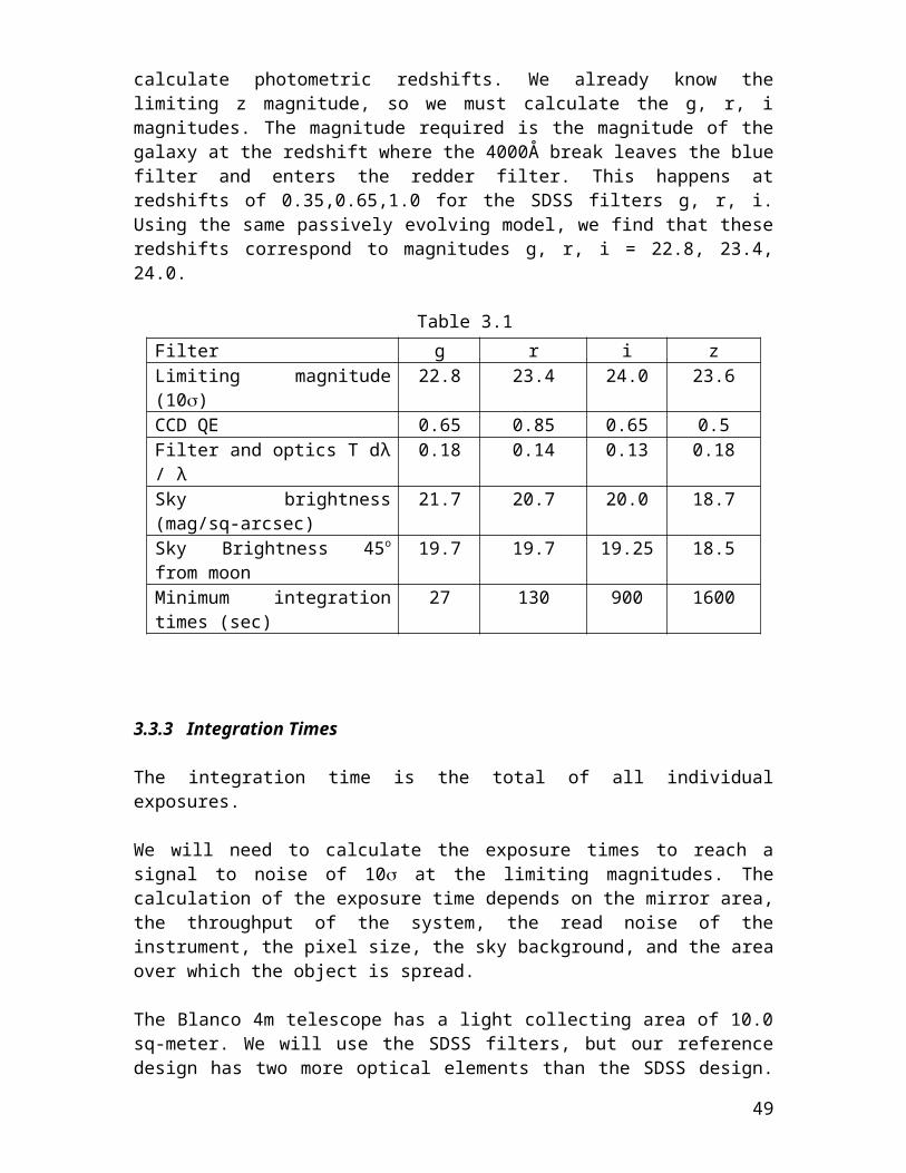
4.5 Cage and Integration

Figure 4.4 shows a detailed view of the cage. The corners of the cage represent the interface to the existing spider. This joint marks the outer mechanical boundary of what we plan to replace. The internal layout of the cage has been designed with ease of servicing in mind. The corrector is supported from the center of the cage. A focusing mechanism is part of the interface between the cage and the corrector. The linear bearings internal to the cage allow the corrector to be separated from the camera and moved towards the primary. This will allow access to the shutter on the camera face and to the filter changing mechanism. Cables and cooling tubes from the floor of the telescope will follow the trusses and spider to the left end of the cage. Development of a clear understanding of the cable and cooling tube routes, and how to deal with the cage rotation, is a critical aspect of the integration of our proposed design with the existing infrastructure at the Blanco. Our Reference Design has the cooling tubes attaching to the left end of the camera vessel and the CCD cable connections on the sides of the vessel.

Figure 4.4. Proposed layout of the prime focus cage with the 2.1 degree corrector, filter changing mechanism, shutter and camera vessel.

A major advantage of replacing the entire cage and all of its service functions is that it minimizes the complexity of the interfaces with the Blanco telescope. In addition, it allows us to assemble the entire camera and all of its services in a self-contained module that can be completely tested before shipment and installation at Cerro-Tololo. This means that the integration effort is localized and is a far simpler task than if the new camera were installed piece by piece into the existing cage. We are also in close contact with our NOAO representative (T. Abbott) for discussions of integration issues and have initiated the construction of a scale model of the telescope and surrounding service areas. As the Reference Design progresses, an integration and configuration control committee will be established to provide the organizational structure necessary for successful integration of the Dark Energy Survey Instrument with the infrastructure on the Blanco.

49

A

AMOSAIC ARRAY B

B

OPTICAL AXIS

SCROLL SHUTTER

MOSAIC CAMERA

CRYO LINES& DEWAR

LONGITUDINAL BRACEOPTICAL FILTER

PRIME FOCUS CAGE OPERATIONAL POSITION

END VIEWFOCUSINGMECHANISMNOT SHOWN IN THIS VIEW

CROSS-SECTION AACROSS-SECTION BB

CORRECTOR LENS ASSEMBLY

FOCUSING MECHANISM

LINEAR BEARING STRUT

LINEAR BEARING

DETECTOR HEAD ELECTRONICS

DETECTOR PLATEFOCAL PLANE

4.5 Optical System

4.5.1 CorrectorPreliminary designs of the corrector were commissioned by NOAO and are currently being evaluated. For the two 2.1 deg. FOV designs, the largest optical elements are ~900 mm in diameter. For our Reference Design we use the concept study by Prime Optics of Eumundi, Australia. The design has 4 elements made of fused silica, as shown in Figure 4.5. The details of the component locations are given in Table 4.2. It is necessary to use lenses with aspherical surfaces on one face of each element to achieve the desired level of image correction over the full field of view. Designs with all-spherical elements exist but require the use of additional elements.  The current design with aspheric surfaces is optimized for wavelengths of 0.4 to 0.9 microns with lateral chromatic aberrations controlled only within the bandpass of each filter. The desired performance is such that D80 (the diameter enclosing 80% of the light) be smaller than 0.6 arcsec at all wavelengths and positions; this value corresponds to a FWHM of order 0.4 arcsec.  This performance is indeed achieved for all wavelengths at all positions except for the 0.4 micron wavelength, which grows to a D80 of 0.8 arcsec in an annulus of width 10 mm at the edge of the field.

Figure 4.5 Reference design for the corrector.

Table 4.2: The Size & Location of Optical Components in the Reference Optical Design for a 2.1 deg. Field of View Camera.

Component Thickness at center (mm)

Diameter (mm)

Distance from Primary (mm)

50

(mm)

C1

C2

C3

Filter

Window and focal plane

C4

C1 70 900 9200C2 80 830 9275C3 35 640 9717Filter 12 560 10458C4 75 540 10483Window 24 480 10730Focal plane 440 10755

The optical design places tight tolerances on the alignment of the lenses.  A preliminary tolerance analysis shows that two of the lenses must be aligned to an accuracy of +/- 30 microns in each dimension.  This accuracy is challenging, but achievable. A preliminary quotation of for the lenses is $2.43M with a delivery of 2 years ARO. Another $500K and 6 months is estimated for building the support barrel and to assemble and align the lenses in the barrel to the required tolerances.

51

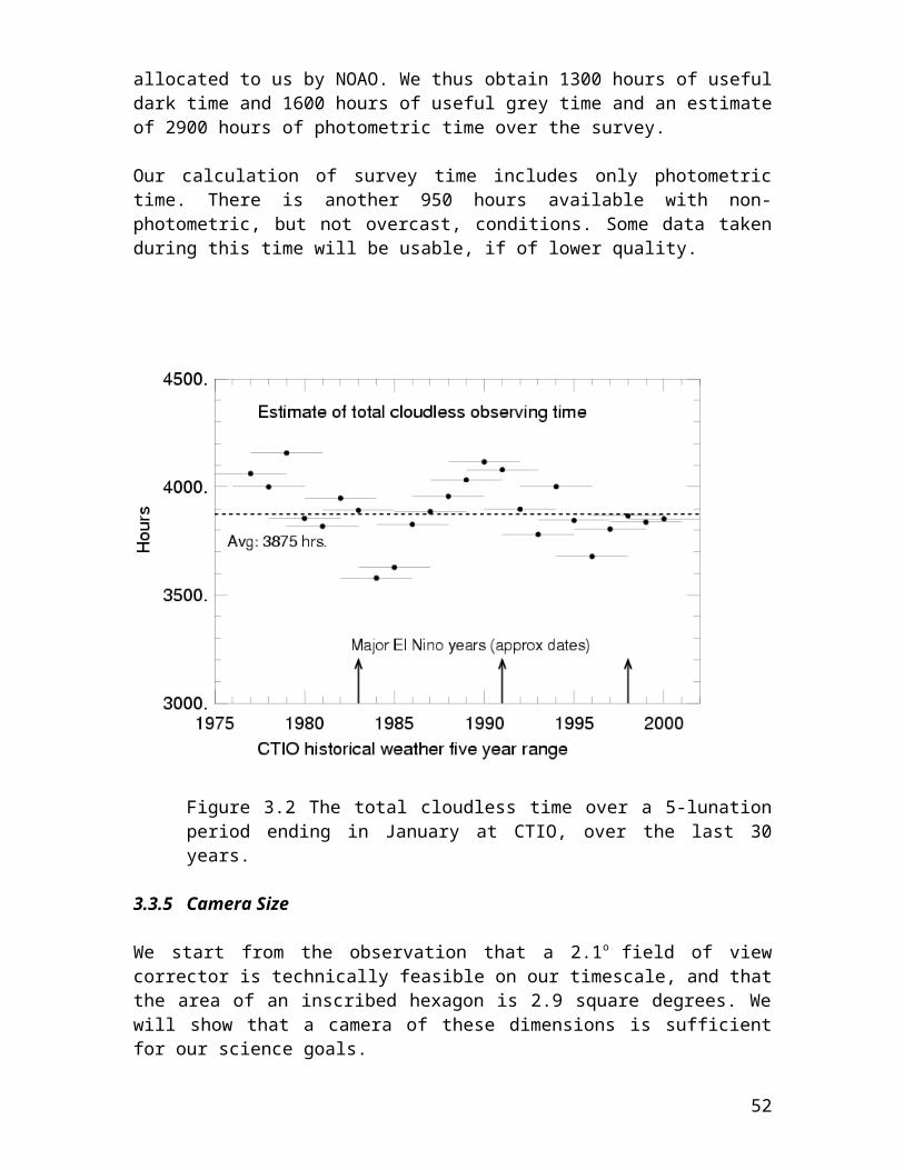
4.5.2 Filter Characteristics

We adopted the SDSS g, r and i filters for our Reference Design since they will provide the required accuracy in the determination of the photometric redshifts of our target galaxies. As noted earlier, our z band red cutoff differs slightly from the SDSS z band. While both are effectively defined by the red cutoff of the silicon, the thick, high resistivity silicon CCDs that we plan to use have a much higher QE in the z band than the SDSS CCDs. The filter characteristics were selected to bracket the Calcium H and K break at 394 nm in the spectrum of red galaxies, which is typical of galaxies in clusters. At 0.05 redshift the H and K break is at 410 nm, just blue-ward of blue cutoff (50%) of the g band filter. At a redshift of 1.1 the break is at 830nm, just red-ward of the red edge (50%) of the i filter. Note that we want filters to bracket both sides of the H and K break in order to derive good photometric redshifts; in particular the z filter is necessary at redshifts near one in order to provide coverage red-ward of the H and K break.  The proposed characteristics of the filters are shown in Table 4.3.

Table 4.3 The Proposed Wavelength Characteristics of the Filters.

Name Center (nm) FWHM (nm) Trans. (%)g 480 140 0.91r 625 140 0.97i 770 150 0.98z 950 240 0.98

4.5.3 Filter Changing System

Typically there will be one or more filter changes per night. For example, when the moon rises, the i and z band observing are not affected, while g and r are significantly degraded. This would motivate a filter change. We are designing a filter changing system which will make it possible to change the filters quickly and reliably. The time estimated for a filter change is 20 sec. and it will be possible to perform a filter change during slewing if necessary. The large space between element C4 and C3 is the optimum location for the filters and the filter changing mechanism. The implications of this choice are 1) these filters are quite large, ~560mm (~22”) diameter and 2) the guide and focus CCDs, which are located on the focal plane with the image CCDs, will see filtered light and thus must also be sensitive in the z band. Our choice for these CCDs will be discussed in section 4.6. We have contacted vendors to determine cost and feasibility of procuring filters this size. Preliminary cost estimates are roughly $100K per filter.

4.5.4 Camera ShutterAnother essential component is the camera shutter. It is desirable to have a relatively fast (compared to the nominal exposure time of 100 sec) and repeatable shutter which results in equal exposure time for all CCDs in the focal plane. Two designs are being considered. A scroll shutter is our Reference Design and is shown in Figure 4.6. This shutter would take a minimum of space in the cage, allowing good access to the corrector, camera and cables. This design is also flexible in that the opening in the scroll could be modified to give very short exposure times. A leaf shutter would fit within the cage, but it would restrict access to the corrector support barrel. Both shutters provide uniform exposure for the CCDs and would include a position sensing system to feedback the precise location of the shutter as it opens or closes.

52

Figure 4.6 Details of the scroll shutter design.

4.6 CCDs , CCD packaging and Front-end Electronics

4.6.1 Pixel Size

The telescope seeing and the pixel size determine the size of a point-like image. Typically this is represented in terms of the FWHM of the point spread function (PSF). While the seeing at the site can be as small as 0.6”, the effective dome seeing with the Mosaic II and its corrector is typically between 0.8” and 1.1”. Given that the Blanco prime focus image scale is 55 microns/arcsec, we selected a pixel size of 15 microns ( 0.27”) for our reference design so that the PSF would be sampled over at least 2 pixels in ideal seeing (0.6”) and 3 pixels in the best recorded seeing (.8”). If smaller pixels were used to provide finer sampling there would only be a small gain in the potential precision of the photometry. The choice of 15-micron pixels makes a very small contribution to the PSF width even in ideal seeing.

4.6.2 CCD Options

Our survey goals require that we have high quantum efficiency (QE) at the near infrared wavelength of ~ 1000 nm. The standard astronomical CCDs typically have a QE at this wavelength of 5-10% because the charge collection region is 10-20 microns thick and the total device thickness is often less than 50 microns. The absorption length in silicon is 205 microns at a wavelength of 1000nm and thus thick sensors are required for a better QE at that wavelength. Photons from the near infrared wavelengths will simply pass through 50 microns of silicon. The SNAP project (led by LBNL) has requirements similar to ours and LBNL has already developed thick, fully depleted, back illuminated

53

A

0.005" STEELSHUTTER BLADE

A

SHUTTER SPOOLB

SHUTTER SPOOL

DRIVE MOTOR

SPOOL BEARING

SPOOL BEARING

DETAIL AND CROSS SECTIONAL VIEW OF SCROLL SHUTTER

CAMERA WINDOWOPENING

SLIT SHUTTER, MID-POINT

CROSS SECTION BB

FULL FIELD SHUTTER,OPEN

CAMERA WINDOWOPENING

CROSS SECTION AA

0.005" STEEL SHUTTER BLADEB

DRIVE MOTOR

TENSIONING SPRING

TENSION SPRING

CCDs 200-300 um thick1. For our Reference Design we use 250 micron thick LBNL CCDs. The QE of the LBNL CCDs is shown in Figure 4.7 and compared to a standard thinned astronomical CCD and a deep-depleted CCD2.

0

10

20

30

40

50

60

70

80

90

100

300 400 500 600 700 800 900 1000 1100

Wavelength (nm)

Qua

ntum

Effi

cien

cy (%

)Thinned CCD Deep Depleted LBNL high resistivity

Figure 4.7 QE curves from different types of CCDs.

LBNL has produced a variety of CCD arrays for different projects and several devices have already been deployed for astronomical use. Figure 4.8 shows a 6” diameter wafer with LBNL CCDs. For our reference design we choose the 4-side buttable 2048 x 4096 CCD. These are the two largest devices shown on the wafer. The development of this CCD is nearly complete and they meet our specifications as shown in Table 4.4. This CCD has 15 micron pixels and 2 readout channels. The readout time is under investigation. These devices have been clocked at 240kps on a probe station at -40oC. At this rate it would take 17.5 sec. to readout a CCD. This is well within the 35sec slew time of the Blanco and thus readout would not introduce additional overhead to the survey.

Figure 4.8 LBNL CCDs on a 6” wafer

54

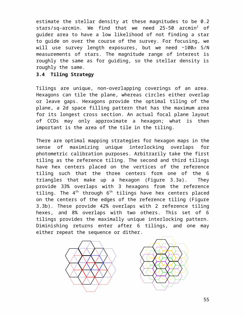
Although we have not ruled out using commercially available CCDs, the overall approach in our reference design is to assume we will use the LBNL thick CCDs. We believe this minimizes the R&D needed for this project by using CCD designs that have already been proven. Currently no commercially available CCDs meet our requirements on QE in the near infrared region.

Figure 4.9 shows our Reference Design for the focal plane layout with the 2K x 4K 4-side buttable LBNL CCDs. It contains 60 CCDs and a total active area of 2.8 deg2. This satisfies the requirements described in Chapter 3 for the camera size.

Table 4.4 CCD Specifications

LBNL CCD performance DECam requirements/Reference Design

Pixel array 2048 x 4096 pixels 2048 x 4096 pixelsPixel size 15 m x 15 m 15 m x 15 m (nominal)

<QE (400-700 nm)> ~70% >60%<QE (700-900 nm)> ~90% >80%<QE (900-1000 nm)> ~60% >50% at 1000 nm

Full well capacity 300,000 e- >100,000 e-

Dark current 2 e-/hr/pixel at –150oC <~25 e-/hr/pixelPersistence Erase mechanism Erase mechanismRead noise 2 e- < 10 e-

Charge Transfer Inefficiency < 10-6 <10-5

Diffusion 8 m < 10 mLinearity Better than 1% 1%

4.6.3 Front-end Electronics

We are evaluating two options for the front-end electronics. This is the system that takes the analog signals directly from the CCD and converts them to digital signals. We later discuss the DAQ system that we define as the CCD control electronics, the conversion of the digital signals to optical and the system that interfaces with the telescope controls for guiding and focus. The choice of a front-end electronics system affects the CCD packaging (discussed in the next subsection).

Our Reference Design uses the CRIC2 chip that is being developed by LBNL for the SNAP project3. This chip is an attractive solution because it can be mounted in the CCD package, enabling signals to be converted to digital at the CCD and thus minimizing the possibility of noise pickup and also reducing the electronics needed outside the camera vessel, inside the cage. Digital signals exit the camera vessel and are converted to optical signals in the cage. The CRIC2 is designed to work at the temperature of the CCD focal planes (~ -120o C). The CRIC chip, which contains just the double correlated sampler, but not the analog to digital converter, has already been made. It was tested at -130o C and meets our signal to noise requirements. Design of the electronics inside and outside the vessel is being investigated.

55

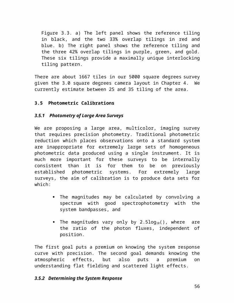
Figure 4.9 Focal plane layout using the 2K x 4K LBNL CCDs and 8 additional small CCDs for guiding and focus.

Our backup front-end electronics option uses the Monsoon front-end system (called Detector Head Electronics or DHE), which is being developed at NOAO as the general purpose CCD readout, and control system. With this system the analog CCD signals exit the camera vessel via cables and feed-throughs. The signals are processed and converted to optical signals in crates mounted in the cage. As discussed in Section 4.8 the readout for our focal plane would require 2 standard VME crates in the cage and these would generate ~ 390 Watts of heat. For our initial CCD test stands we will use the Monsoon DAQ system with the Monsoon DHE. This is described in more detail in Section 4.8.

4.6.4 CCD Packaging

CCD packaging is the act of gluing a readout board and a thermal/mechanical interface to the front of the CCD. A picture of a packaged CCD is shown in Figure 4.10. The readout board is made of Aluminum Nitride (AlN) and contains bond pads, for wire bonding to the CCD, and a connector for a cable. A piece of molybdenum (Mo) or Invar, called the foot, is glued to the board to provide the precision alignment features, thermal contact with the cooling plate as well as stiffness for the CCD package. In the case of the CRIC2 front-end system, the readout board also contains the circuitry for operation and control of the CRIC2 chip and the mechanical foot has to allow additional space for the chip and circuitry.

56

Figure 4.10 A picture of a packaged 2K x 4K CCD4.

CCDs are typically operated at temperatures of -90 to -120 deg. C, however, they must be glued to the support and readout boards at approximately room temperature. This wide temperature difference requires careful consideration of the thermal expansion properties of all the materials involved, as flatness of the focal plane is important for the camera to achieve a good focus. As described in Reference 4, development of a packaging process for the 2K x 4K CCDs is well underway at LBNL. In particular, AlN has been selected for the material of the readout board and Mo or Invar have been shown to be good materials to match the thermal expansion properties of the CCDs.

For construction of our camera, we need to develop packaging techniques and establish a production model at Fermilab that can handle a large number of CCDs. The Silicon Detector Facility at Fermilab already has significant expertise in bonding and gluing ceramic parts to silicon sensors as a result of the construction of the numerous silicon vertex detectors for the collider program. We believe that CCD packaging will be a natural extension of that experience. In the next few months we would like to begin pursuing CCD packaging at Fermilab with the 2K x 4K CCDs and the Monsoon front-end electronics. In Section 4.9 we outline this program and the resources needed to support this effort. Our aim is to be ready to place a production order for the CCDs by June of 2005.

4.6.5 Focus CCDs

Focusing of the Blanco with Mosaic II is somewhat time consuming (~10 min) and thus is typically performed only 2 or 3 times per night. It involves taking a series of images and determining which has the best focus. We plan to design a semi-automatic focus system that can be used more often, without adding to the observing overhead. This consists of two sets of focus chips installed above and below the ideal focal plane. As the telescope drifts out of focus for the image CCDs, the focus in one or the other set of focus chips will get better. The focus chips are readout with the image CCDs. The focus is thus monitored on every image and can be adjusted as necessary.

As discussed in Chapter 3, an area of ~40 sq. arcmin would typically have ~three bright stars which are useable for focusing. The vertical offset of the focus CCDs with respect to the focal plane will depend somewhat on the corrector optics and the desired defocusing of the images. Using the f-ratio of the primary and the assumption that we want a 0.7 arcsec image to double, we find that the focus CCDs should be ~200 microns from the best focus of the focal plane. LBNL has developed a variety of small CCD options. For our Reference Design we have selected a 982x935 device with 15 micron

57

pixels. Each CCD covers 18.6 sq. arcmin and has two readout channels. Four of these CCDs would be used for the focusing system.

4.6.6 Guide CCDs

The Mosaic II has a two guide cameras in addition to the main image CCDs. The guide cameras provide small corrections for the telescope tracking system such that a star image will stay in precisely the same location during an exposure. The Blanco accepts these signals every 2 sec. In our reference design we have CCDs on the focal plane devoted to guiding.

Guide CCDs have two requirements in addition to those listed in Table 4.4. These are a fast readout rate (<~1sec) and the possibility to operate in frame-store mode. The fast readout rate is needed so that corrections to the telescope position can be generated on a time scale that matches the 2 sec. update rate accepted by the Blanco control system. This faster rate also implies a separate DAQ path for the guide CCDs and this is discussed in section 4.8.

Frame-store mode is a technique for collecting clean images without the use of a shutter. This is accomplished by coating one half of the CCD with an opaque layer and collecting the image only in the other half. The image can be transferred very quickly (~1ms) from the image side to the storage side. This minimizes smearing the image during the readout. Once an image is on the storage side, the image side is erased, a new image is initiated and the readout can occur from the storage area of the CCD.

The CCDs described above for focusing are also a good match for our guiding requirements. To cover the desired area we would need 4 of these CCDs (note only half of each CCD is used to collect the images). A readout rate of 240kpix/sec would result in a readout time of ~0.9 sec. Figure 4.9 shows 4 guide and 4 focus CCDs along the top and bottom of the focal plane layout. There is room for additional guide/focus CCDs if they are needed for redundancy.

4.7 Camera Vessel and Cooling

This section describes the vacuum vessel that houses the CCD focal plane and all the associated cooling and mechanical components. The CCDs will be precisely located and attached to a large metallic plate called the focal plate. This plate defines the interface between the CCDs and the camera vessel. To achieve the low noise necessary for astronomical applications, the CCDs are typically cooled to -90 to -120 deg. C. For our Reference Design we assume they need to be cooled to -120 deg. C, although we will investigate running them at warmer temperatures. The focal plate will be thermally coupled through copper braids to a cold mass that is directly cooled by an LN2 volume (the cryostat) internal to the vacuum vessel. Small heating elements will be used to actively regulate the temperature of the focal plate. Good vacuum in the vessel is needed to minimize the thermal load from the ambient environment.

Figure 4.11 shows a sketch of the layout of the cooling system within the vacuum vessel. The vacuum vessel (the camera) will be mounted on the end of the corrector. Mechanical support of the focal plate will be from the window end of the vacuum vessel; thermal insulators will be used to minimize the heat transfer from the vessel walls to the focal

58

plate. The heat load on the cooling system comes primarily from the ambient environment through the vessel window (~100 W), and the CCD’s and the associated electronics (~20 W). Feed-throughs and resistive losses along the cables will add an additional load. For our Reference Design we have chosen a cooling system capable of removing 200 W from the vessel.

The cryostat shown in Figure 4.11 would be either continuously or automatically batch filled. Two inputs and outputs will be located in the cryostat to allow proper filling and venting at the different telescope angles. The LN2 will be delivered to the prime focus cage in vacuum insulated piping with flexible joints to allow for the rotation of the cage.

Figure 4.11 Schematic view of the Dark Energy Camera Vacuum vessel. The heat load from the cables is intercepted at the cold station near the LN2 vessel. Zeolite is a getter material which will help maintain a good vacuum. The two sets of supply and return lines are located at different heights to accommodate the tipping of the telescope.

Although liquid nitrogen is available from the plant at the Blanco, we are pursuing using a nitrogen recondenser system. A schematic of the system is shown in Figure 4.12. A helium cold finger pulse tube is mounted to the top of each recondensing dewar. The returning warm gas is delivered to the cold finger and condenses on it, dripping down into the recondensing dewar. The liquid nitrogen supply to the camera comes from the bottom of these dewars. We estimate two 210 liter recondensing dewars are needed. This system has no moving parts in the primary cage, a big advantage in terms of operations, maintenance and minimization of vibrations. The helium compressors and the recondensing dewars would be mounted either on the floor of the telescope platform, or in the area around the Cassegrain focus. A backup dewar would be used in case of failures. Ideally this system would be filled with LN2 only once and require little or no refilling. Discussions with NOAO are in progress to determine possible locations for the recondensing dewars, and the length and paths of the piping.

59

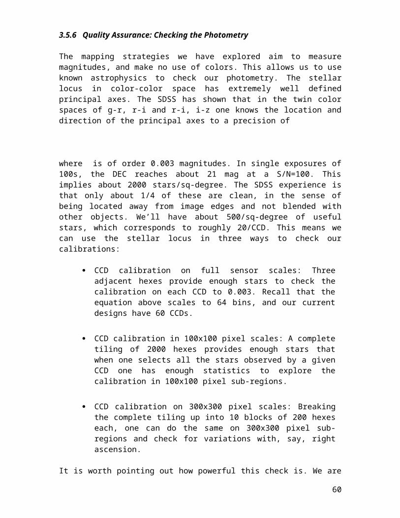
Figure 4.12 The schematic layout of the LN2 recondenser system with two 210 liter recondensing dewars and one passive 180 liter back up dewar for emergencies.

4.8 Data Acquisition

This section describes the data processing system that resides outside the vacuum vessel. The interfaces to this system are the cable feed-through ports on the vacuum vessel and the optical cables/signals that are delivered to the data management system in the telescope control room.

The data acquisition (DAQ) serves two functions. One is to convey data from the sensors to permanent storage for subsequent off-line analysis. The other is to monitor and control the telescope and environmental parameters that determine image quality. The DAQ contains both hardware and software components. It must be able to respond to commands issued by the personnel operating the telescope. It must also be able to operate autonomously, maintaining optimal telescope behavior during routine operations and responding appropriately to abnormal conditions.

The data acquisition will be a collaborative endeavor led by the University of Illinois and involving Fermilab and NOAO. NOAO has developed a data acquisition framework, called Monsoon5, which we propose to adapt to this project. This approach carries two advantages over a new design. It reduces the cost and time to completion of the project by taking advantage of previous work. It also maintains and extends a standard for astronomical data acquisition, reducing the costs of future projects.

4.8.1 Data Acquisition Architecture

Our Reference Design uses the CRIC2 chip for the front-end electronics. The CRIC2 is mounted directly on the CCD package and converts the CCD signals to digital before they exit the camera vessel. However, for the upcoming R&D efforts, we will employ the

60

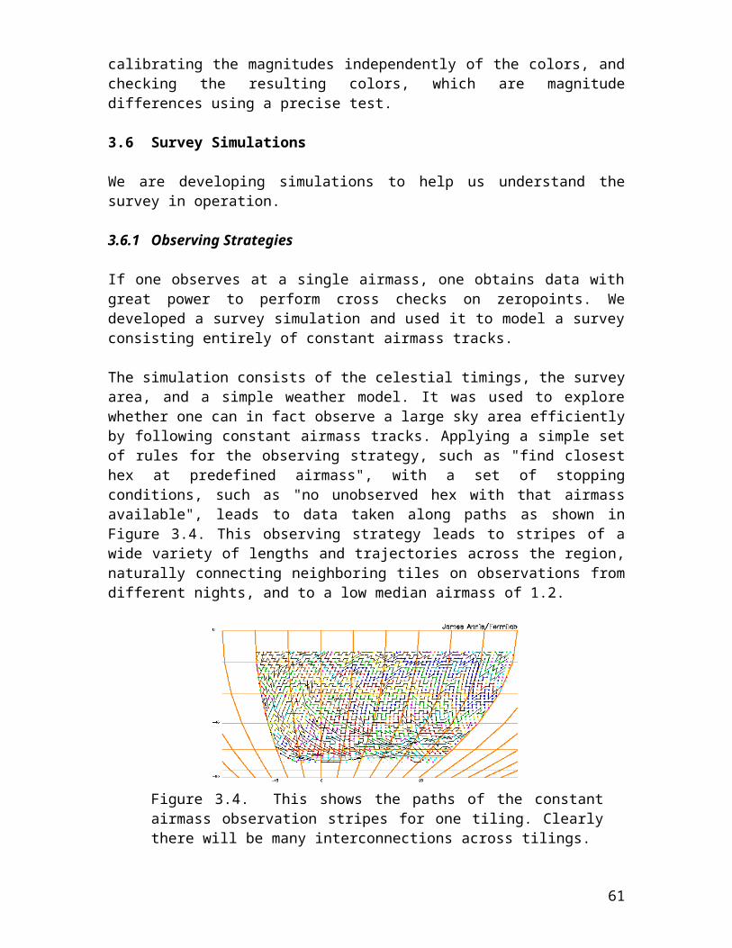
Monsoon system with its detector head electronics (DHE) instead of the CRIC2 chip. Development of Monsoon DHE system also serves as a fall back data acquisition system in case the CRIC2 is not available on our time scale. We take the CRIC2 as our Reference Design because it significantly reduces the electronics mounted in the primary cage. The heat from the front end electronics must be minimized and dissipated carefully in order to avoid creating thermal gradients (and thus distortions) in the primary light path. CRIC2 also has the advantage of converting the analog CCD signals to digital right at the CCD, thus minimizing the chances of noise pickup in the cables. The CRIC2 system has sufficient advantages, particularly for a large mosaic array such as the one we are proposing, that we hope to be able to use it in our camera. Below we will first describe the DAQ architecture with the CRIC2 and then discuss our testing and backup solution with the Monsoon DHE.

The DAQ architecture with the CRIC2 is shown in Figure 4.13 and the important parameters are listed in Table 4.5. Figure 4.14 shows the architecture with the Monsoon DHE. The data rate is high by astronomical standards, but is not beyond what particle physics experiments routinely achieve. For organizational purposes, electronics on the telescope is considered to be part of the front-end subsystem. The DAQ includes hardware and software that resides off-telescope.

Table 4.5 Data Acquisition Parameters

Image CCD ArrayNumber of CCDs 60 (+4 focus CCDs)Pixels per CCD 2048x4096Amplifiers per CCD 2Pixel digitization rate 240 kHzDigitization time 17.5 sBytes per image 1.0x109 Image data rate 10 MB/s (@ one image per 100s)

Guide CCD arrayNumber of CCDs 4Pixels per CCD 982 x 935Amplifiers per CCD 2Pixel digitization rate 240 khzDigitization time 0.9 secBytes per guide 5.8x106 Guide data rate 5.8 MB/s (@ one guide per second)

The DAQ will accept digitized CCD pixel information and deliver it to permanent storage for further processing. Real time processing will include using guide stars to control the telescope pointing. There will be two readout sequences, one for the image and focus CCDs and one for the guide CCDs.

During construction, the DAQ will be used as a test stand, first to test individual CCDs as they are fabricated, then to debug the focal plane before installation on the telescope.

61

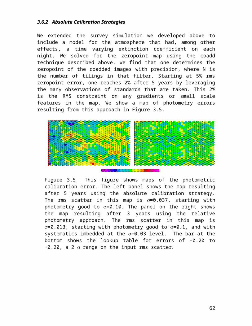
Thus, the DAQ will be completed well before installation.

4.8.2 DAQ Implementation with CRIC2

Although Monsoon is a working data acquisition framework and implementation, we must make significant changes to accommodate our hardware configuration:

Signal digitization will be performed on the focal plane, by the LBNL CRIC2 electronics.

The CCDs will be read out at two different rates, one for telescope guiding, and one for image acquisition.

Telescope

Focal plane image sensors and ADCs

Focal plane guide sensors and ADCs

Dewar wall

electrical

Digital data

Analog and digital controls

Power supplies andelectrical/optical interface

Telescope control and monitoring

Control room

Two Monsoon PANs Monsoon supervisor

Data storage andoffline processing

Two Monsoon DHEs

Fiber optics Fiber optics

Figure 4.13 Block diagram of data and control signal flow for our Reference Design. The CCD signals are converted to digital with the CRIC2, inside the camera vessel.

4.8.2.1 HardwareAlthough we will use the CRIC2 for the front end electronics, the rest of the Monsoon configuration will need to be implemented. This includes two DHE crates, each with a Master Control Board, a Clock/Bias Board, and several Acquisition boards. The system also requires a Pixel Acquisition Node (PAN) PC and a Supervisor PC.

The use of the CRIC2 obviates digitization in the Monsoon detector head electronics (DHE). As a consequence, the DHE Acquisition cards will be redesigned and greatly simplified. They will become digital buffers.

62

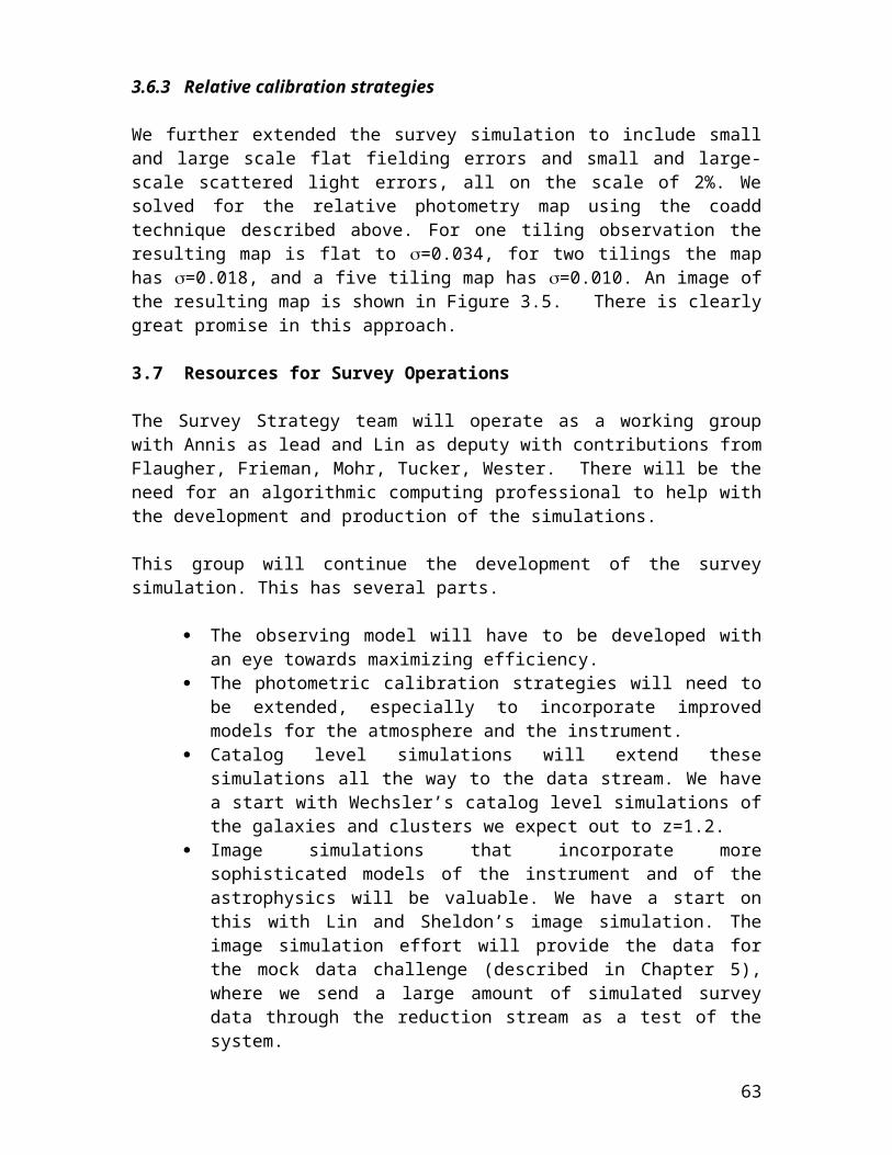
The Clock/Bias Boards generate the digital control signals and analog voltages for the CCD focal plane array. We must redesign them to accommodate the LBNL CCDs. The functionality will be split in two: a card in the DHE crate will generate digital control signals that electronics on the telescope (part of the front-end) will turn into the analog signals needed for the CCD readout.

The on-cage interface converts the electrical data signals to optical for transmission off the telescope. It also receives isolated AC power from off-telescope and generates the appropriate DC voltages. We will design a system that is safe against lightning and other electrical supply interrupts

Control room

Monsoon PAN

Monsoon PAN Monsoon supervisor

Data storage andoffline processing

Telescope

Dewar wall

Focal planeguide sensors

Monsoon DHE

Focal planeimage sensors

Monsoon DHE

Telescope controland monitoring

Optical

Electrical

Digitaldata

Analog anddigitalcontrols

Optical

Digitalcontrols

Digitaldata

Figure 4.14 DAQ architecture with Monsoon DHE

4.8.2.2 SoftwareWe must adapt the existing software to the needs of our project. For example, the DAQ will actively control telescope pointing (on a one second time scale) during exposure. The real-time software must measure the centroids of stars imaged by the guide CCDs and send commands to the telescope controls. Also, CCD diagnostics must be developed for the test stand application. These diagnostics will then be modified for use as focal plane monitors on the telescope.

4.8.3 Backup design: DAQ Architecture with Monsoon

Monsoon is a working data acquisition framework and implementation, and is already

63

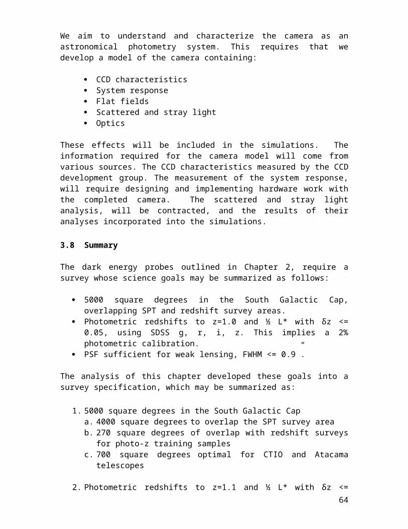
being implemented for use in the NEWFIRM project. We could to use it with minor modifications. The most significant would be the use of higher density ACQ cards, currently under development. The existing ACQ cards have 8 channels each. Our space estimates assume 16 (but we assume no cost or power reduction). The higher density is needed to fit the DHE electronics into two crates on the telescope, where space is at a premium. In order to make two crates meet our needs, one crate must have a split backplane. This allows the guide CCD DAQ to share a crate with the image CCD DAQ. The cost of the DAQ is calculated by scaling the NEWFIRM channel count and including the modifications described above. The total power is estimated at 390 W and this needs to be dissipated in the primary cage. The total cost for an implementation for our the backup DAQ architecture is $280K.

4.9 Resources Requests

We have presented our Reference Design for the Dark Energy Survey Instrument. This would replace the existing cage on the Blanco 4m telescope and everything inside it as well as the interfaces from cage to the off-telescope systems. Our Reference Design meets the technical requirements of our science program and its major characteristics are summarized here:

1) a 2.1 degree angular field of view corrector 2) a set of four filters in the g, r, i and a modified z bands3) high purity thick CCDs which have a high QE in the i and z band4) a focal plane of 60 2K x 4K CCDs with a pixel size of 15 microns and 2 readout

channels per CCD5) Guide and focus chips (4 each) on the focal plane, these are 982 x 935 and have a

pixel size of 15 microns6) Use of the CRIC2 for front-end electronics with a Monsoon DAQ system7) A cooling system for the CCDs which uses a liquid nitrogen recondenser8) Packaging of the CCDs will occur at Fermilab.

While not required by the science goals, the decision to package the CCDs at Fermilab gives us more control over the cash flow and schedule than if the CCDs were packaged elsewhere and capitalizes on the experience and facilities already in existence at SiDet.

We do not expect to change our science goals, nevertheless some of the choices that were made to implement them are not final and may change, particularly if we discover faster and less expensive solutions.

We have developed a preliminary schedule based on physicist and engineering estimates for the Reference Design. The project summary information is given in Table 4.6. The material and service costs of the resource estimates are given in FY04 dollars and the estimate for the effort is given in terms of FTEs. The latter is further divided into skill types such as engineers, scientists, and technicians as shown in Table 4.7. The preliminary estimate of the project duration is ~ 3.5 years. We define one FTE-yr to be 2000 hours of effort per year and note this does not include any efficiency factors or contingency. While we believe that the WBS for the Dark Energy Survey Instrument is reasonably complete, the cost and labor estimates are preliminary. For this reason we present our base estimates without contingency. We expect to improve the accuracy of these estimates once we have finished a complete preliminary engineering design. Our

64

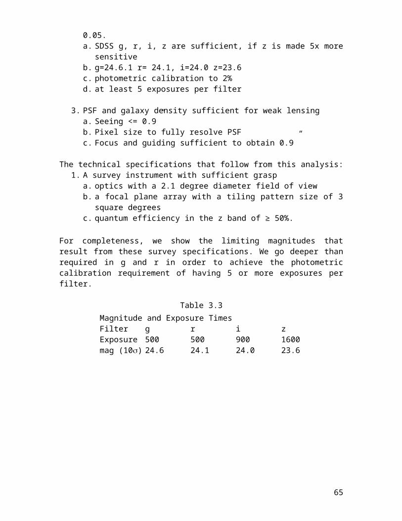
goal is to complete the initial pass on this design in May of this year and to have an external review of the project soon thereafter.

Table 4.6 Preliminary WBS for the Dark Survey Instrument

    M&S ($K) Labor FTE-yr1.2 Dark Energy Instrument $6,672.00 32.51.2.1 CCDs and Test Stations 1,347.00 2.61.2.2 CCD Packaging and Testing 592.00 11.41.2.3 Corrector and Cage 3,659.00 4.91.2.4 Camera 590.00 6.91.2.5 Data Acquisition 334.00 1.6

1.2.6 Final Assembly 130.00 4.8

1.2.7 Models 20.00 0.4

Table 4.7 Preliminary Labor Estimates for the Dark Survey Instrument

  Labor (FTE-yr)Electrical Engineer 3.0Mechanical Engineer 8.2Scientist 13.7MechTech 5.7Draft 1.3ElecTech 0.7

The main cost and schedule drivers are the optical system, which amounts to $3.7M, and the CCD procurement and packaging, which sums to $1.9M. We estimate that each will take approximately two years to complete. The optical system and the CCDs currently define two technically independent critical paths in the schedule and we hope to discover less expensive, quicker ways of implementing our technical requirements. Since we recognize that minimization of the cost of this project is critical to its timely completion, we have developed a plan for optimizing our design. This is described in section 4.9.1 along with a summary of the resources needed to initiate this plan in the next 3 quarters (Table 4.8).

4.9.1 Design Optimization Program

This section identifies cost and schedule risks in the project and outlines our plans to minimize them. We will be investigating our options for simplifying the design and are avoiding any research and development.

4.9.1.1 Optical designTwo preliminary designs for a 2.1 degree corrector were commissioned by NOAO and one of these has been adopted for our Reference Design. For this design we have received one preliminary quotation of $2.53M for the lenses with a 2 year delivery. The aspheric surfaces in this design are responsible for both the cost and the extended schedule. In the next few months we plan to obtain quotes from other vendors and to

65

explore alternative designs with the goal of reducing the cost without sacrificing functionality. While some optical expertise exists within our group, it is in our interest to establish a contract with an optical designer/engineer as soon as possible. This designer/engineer would be supervised by the leader of our optical design coordinator (S. Kent). Together they will work though possible changes to improve and simplify the design. Another important aspect of this analysis is a full tolerancing of the design. This will provide specifications for the lens-to-lens alignment and have a significant impact on the cost of the lens support structure. Very preliminary estimates for the corrector barrel are that it will take ~$500K to build and ~6 months to assemble and align the lenses in the barrel once they are completed.

The long lead-time for the corrector is a significant schedule risk for the project. To reduce this risk we would like to get a rapid start on the optical design by establishing a contract with an optical designer beginning in May 2004. Our understanding is that the first 6 months of the 2 year corrector delivery is to obtain the rough pieces of glass. The remaining 1.5 years are for grinding, polishing and testing. We would like to order the glass for corrector lenses ($320K) in Nov. 04, after a complete review of the corrector and barrel designs.

4.9.1.2 CCDs and CCD packagingAs discussed in section 4.6, we need high purity, thick CCDs to obtain a high QE in the z band. Currently no commercial vendor is offering such a product. However, LBNL has developed CCDs that meet our needs. These have already been produced and packaged in small quantities4 and are in use in telescopes at Kitt Peak National Observatory with great success. LBNL has established a production model for CCD fabrication in which the silicon wafers are manufactured at a commercial vendor and then delivered to LBNL for final processing. We have initiated discussions with LBNL about the CCD procurement and delivery and believe we have reached a good first draft of the cost and schedule. In our model, LBNL would receive the wafers from the foundary, perform the final processing and then ship unpackaged, untested devices to Fermilab for packaging and testing. We have avoided extensive development on the CCDs by basing our plans on the existing 2K x 4K design. However, the CCDs have a lead time of approximately 10 months for delivery of processed unpackaged CCDs. Our experience with the construction of silicon vertex detectors leads us to believe that it will require a modest dedicated effort to develop CCD packaging skills and techniques at Fermilab and to develop an efficient CCD packaging production line. We would like to begin this process as soon as possible to reduce the possible risks later in the project.

Our CCD acquisition strategy proceeds in 4 phases:

Phase A: May 04, order mechanical parts for packaging studies, a few unpackaged electrical CCDs and one fully packaged CCD, ~3 m delivery

Phase B: July 04, order preproduction parts and process ~6 wafers, est. 10 m delivery

Phase C: June 05, process the remaining wafers, ~3 m delivery Phase D: June 05, place production order, ~9 m delivery

Phase A is the purchase of large number of mechanical CCDs (blank silicon with the top layer of metal for wirebonding studies), as well as one packaged CCD and a small quantity of unpackaged devices. We would like to proceed with this purchase in May

66

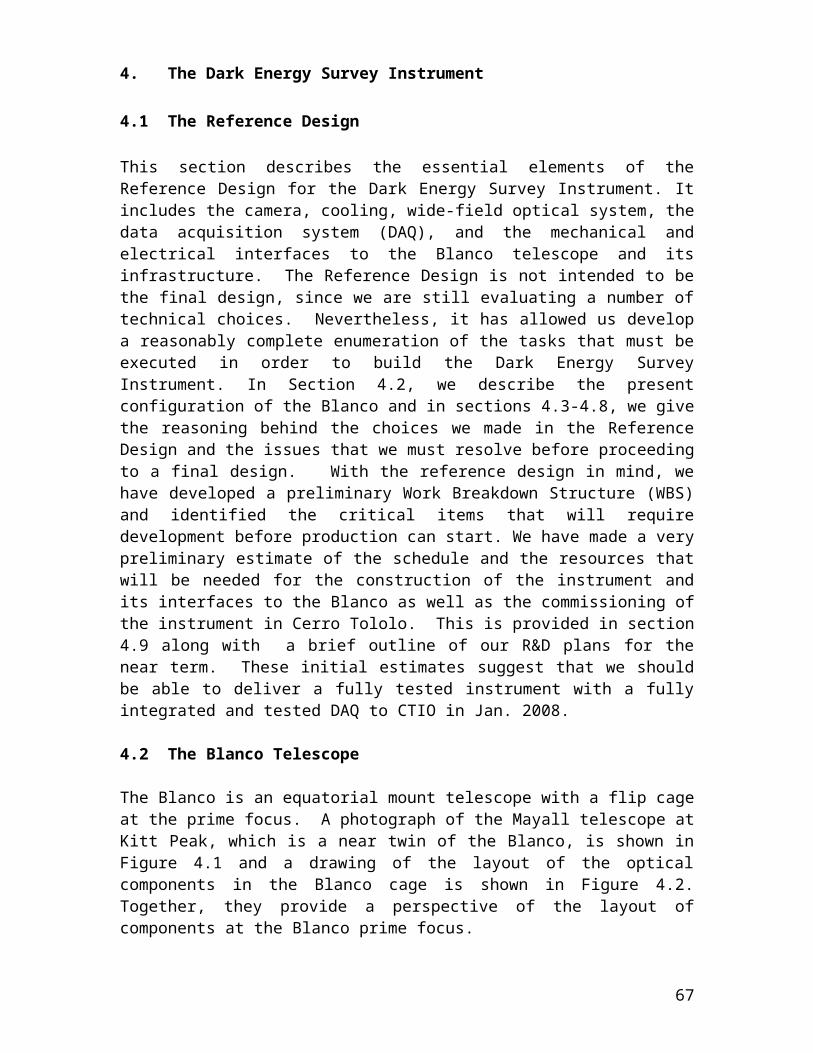
2004 so that we can begin to develop our packaging and testing facilities at SiDet.

The initiation of Phase B (preproduction) is on the critical path for the project and is a key step towards reducing both cost and schedule risk. In Phase B we ask LBNL to generate the preproduction masks for our project and place an initial minimum order for 24 wafers. The existing masks for the 2K x 4K CCDs have only two of these devices per wafer. The new mask would use the same, proven, 2K x 4K CCD design and would have four devices per wafer. Our goal is to start the new mask design in May 2004 and place the preproduction wafer order in July 2004. The delivery schedule is ~10 months after the masks have been approved by the foundry. On receipt of these wafers (~April 05) we would have LBNL process only ~6 for use in our CCD packaging studies. These would be evaluated and tested with the goal of placing the production order in June 05. The remainder of the wafers would be set aside for phase C.

In Phase C we would authorize LBNL to process the wafers that were set aside in Phase B. Since the wafers would already be at LBNL, the delivery of these would be quick, ~3 months ARO. These CCDs would arrive at FNAL in ~Oct. 05 and would be used to start the ramp up to full production packaging. We estimate that 10 wafers would be left, yielding ~40 untested unpackaged CCDs. Our goal would be to package these at an average rate of ~2/week. We will also investigate the value (and potential losses due to handling) of performing initial tests on a -40 deg. C probe station (with the existing equipment at SiDet) to eliminate obviously bad CCDs before packaging.

The final phase, D, is the production run of 72 wafers. Unless significant problems were found from the preproduction run, this would use the preproduction wafer mask. For our initial planning purposes we assume that we will need to receive and package a total of 160 CCDs from LBNL to allow for the yield (initial estimate is ~50%) and to have some spares. This order would be placed in June 05 with the delivery schedule estimated at 7-9 months. Initially, to minimize costs, we would have LBNL process only 30 wafers. Once full production has been established, we assume we can package and test 120 CCDs at a rate of 4/week. The Camera Team anticipates having the CCDs ready to mount on the focal plane in Feb. 2007 with the goal of having the camera ready for first light in Chile in Jan.2008.

For development of the packaging process we will need nominal support for engineering, designing and implementing the concepts. This includes purchasing adhesives, samples of Invar and Molybdenum as well as gluing and wirebonding fixtures. In order to prove our packaging techniques are successful, we must operate the CCDs at cryogenic temperatures. This will allow us to observe possible stress points or defects in the process. For this we need a cryostat, a cooling system and the appropriate data acquisition system. We are also investigating a warm (-40 deg. C) CCD testing setup. This would allow faster turn around, as the cool down time would be significantly reduced. Accumulation of this apparatus and knowledge gained from operating CCDs could also be of benefit to other projects at Fermilab; both the LHC and the NLC are investigating CCDs as a possible technology choice for a vertex detector.

67

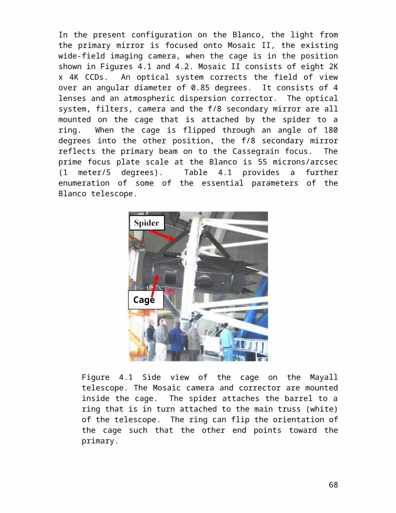
4.9.3 Design Optimization costs for the next 3 quarters

In Table 4.8 we show a breakdown of the M&S costs we will incur in the next three quarters, and Table 4.9 shows a breakdown of the labor by type. To estimate the number of FTEs, we assumed 500 hours/quarter; this does not include any efficiency factors or contingency. These tables cover the labor and costs of preparation of the proposal for NOAO as well as for initiating a contract with an optical designer, placing the CCD purchases and developing a CCD packaging and testing setup as described above. Our schedule for the optical design and the CCDs is aggressive in terms startup and placing the orders on a short time scale, but it is conservative in terms of technology choices. In particular, the CCD plan outlined above has built in flexibility later in the project with the use of the wafers that remain from Phase B and from the production order.

Table 4.8 Detailed cost Breakdown for FY04 and the First Quarter in FY05

   FY04 - Q3

($K)FY04-Q4

($K)FY05-Q1

($K)1.2 Dark Energy Instrument 105.43 218.88 512.11 1.2.1 CCDs and Test Stations 77.41 177.11 11.31

1.2.2 CCD Packaging and Testing 10.02 15.27 35.56

1.2.3 Corrector and Cage 0.00 13.33 359.10

1.2.4 Camera 0.00 4.17 18.59

1.2.5 Data Acquisition 13.00 9.00 79.13

1.2.6 Final Assembly 0.00 0.00 0.00

1.2.7 Models 5.00 0.00 8.42

Table 4.9 Preliminary Estimate of Labor Resources

Labor in FTEs FY04 - Q3 FY04 - Q4 FY05 – Q1Electrical Engineer 1.0 1.2 1.3

Mechanical Engineer 1.9 2.5 2.5

Scientist 2.1 3.7 4.4

MechTech 0.3 0.9 1.1

Draft 1.3 1.0 0.9

ElecTech 0.1 0.2 0.5

4.10 Summary

We have described a preliminary Reference Design for the Dark Energy Survey Instrument that meets our technical specifications and presented estimates of the cost and labor for the project. The critical path items are the 2.1 deg FOV corrector and the CCDs. In the next few months we need to refine our optical design and begin to research the issues related to reading out, packaging and procuring the CCDs. Constructing a

68

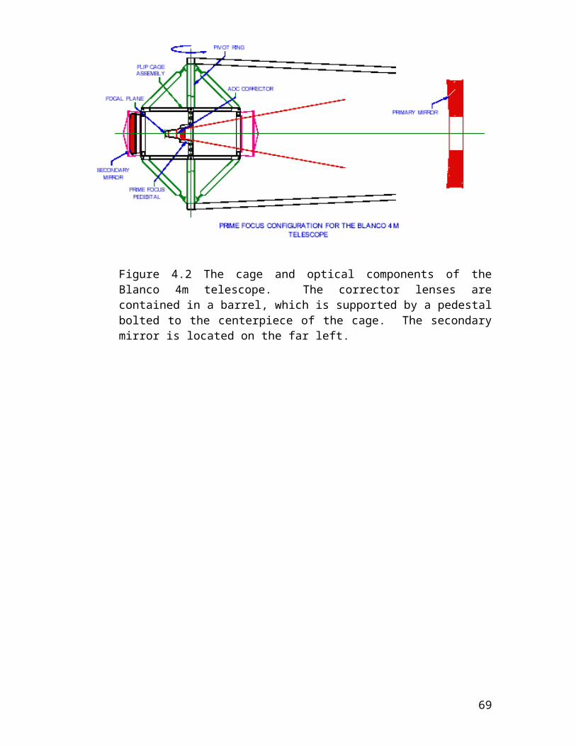
CCD focal plane is similar in many ways to the construction of a silicon vertex detector and the facilities at the Silicon Detector Facility (SiDet) are well matched to these purposes. Initiation of this project will require resources both in terms of labor and the purchase of some equipment as outlined above. These purchases could benefit future efforts at Fermilab as CCDs are currently being considered for future detectors at the NLC.

References

1) S.E. Holland, D.E. Groom, N.P. Palaio, R. J. Stover, and M. Wei, "Fully Depleted, Back-Illuminated Charge-Coupled Devices Fabricated on High-Resisitivity Silicon," IEEE Trans. Electron Dev. 50 (3), 225--238 (January 2003)

2) Plot take from “An Assessment of the Optical Detector Systems for the W.M. Keck Observatory,” by J. Beletic, R. Stover, and K. Taylor (January 2001).

3) J.P. Walder, et al, "A Low-Power, Wide Dynamic Range, Multi-Gain Signal Processor for the SNAP CCD "to be published in Proceedings of the Nuclear Science Symposium, October 2003.

4) To be published in SPIE, H. Oluseyi et al, “LBNL 4-side Buttable CCD Package Development”.

5) Monsoon CCD readout system developed by NOAO.

69

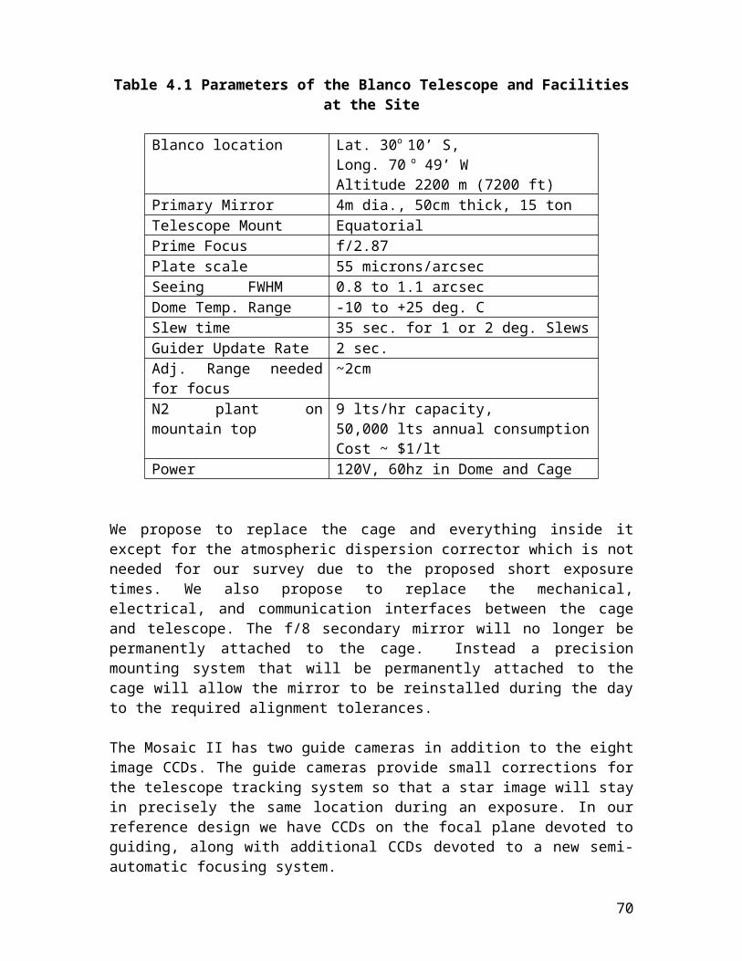
5. Data Management

The four bands from this 5000 square degrees survey will produce roughly 100 TB of imaging data over 600 nights of observing. These data must be efficiently reduced, analyzed for the constraints on dark energy, archived and made available to the public astrophysics community.

The survey data management includes:

moving data from La Serena to processing and archiving platforms, ingesting data into an archive, processing the data within an automated pipeline, formatting, organizing, and transmitting datasets for long-term storage and near-

term access, presenting the data to users via an archive interface, and reviewing data products for quality and scientific integrity.

We consider it our obligation to make our data available in a form that will benefit the astronomy community at large.

The University of Illinois Astronomy group, which will be supported by the National Center for Supercomputing Applications (NCSA), proposes to take the leadership of data management and archiving. The data management endeavor as a whole will be collaborative, involving Fermilab, University of Chicago, NOAO and LBL. Our data plan must address not only the technical issues of data handling across the sites, but also the issues of distributed software and system development. Our data plan aims to leverage efficiently the expertise and resources from the participating sites.

Fermilab will play a major role in supporting data management, specializing in the following areas:

Data simulation and system verification via a mock data challenge. Algorithms for producing science data products (particularly in the area of galaxy

cluster detection and photometric redshifts). Grid-based processing framework.

This work will be done in close collaboration with UIUC and our other partners, sharing development and leverage the expertise and resources at all sites.

5.1. Requirements

5.1.1 Data Products and Data Storage

The raw data products coming from the telescope will be images dumped from the CCDs in the camera after exposure. We will produce roughly 100 TB of raw imaging data over the course of the survey. These must be calibrated to remove instrumental response. The calibrated images themselves will be of value to the astronomy community as the basis for research that outside the scope of our science goals; thus, they can be released as a “level 0” product.

70

The primary product that will form the foundation for the science—the level one product—will be a set of four images, one for each band, with single image scale calibrations, covering the entire survey region.

The level two product will be the data formed and calibrated from the co-addition/mosaicing of all the data from the survey. From these images, we will produce a set of higher level (level three) products, primarily catalogs that will be the subject of scientific analysis. Most notable of these catalogs will be a full object catalog (listing photometry and positions for all detected objects in the survey), a photometric-redshift catalog (containing photometry and redshifts for all galaxies detected), and a galaxy cluster catalog; these form the level 4 products.

Experience from the Sloan survey shows that data processing actually expands the data collection dramatically rather than reduces it. We estimate that after the first year we will need to house roughly 100 TB. By the end of the project, this will approach 1 Petabyte, though much of this can reside in secondary storage (i.e. tape).

5.1.2 Processing Requirements

Our initial estimates of the processing needed to produce our various data products are modest: approximately 10000 hours on a highly parallel platform. An additional factor of 2 maybe necessary to account for reprocessing to correct deficiencies discovered in the course of observations. However in addition to this base level necessary to produce our science data, a significant amount of processing—roughly of the same order—will be necessary during the software development phase. Simulations of the data will be critical for design and testing of the processing software. We estimate that we will need access to the order of 100 compute nodes during both the simulation and production processing phases of the project. 5.2 System and Software Architecture In this section, we outline the system and software architecture necessary to create and support the necessary science data products. Figure 5.1 illustrates the overall data flow. All products—raw and processed—will be archived at NCSA. Our model allows some or all of the archive to be replicated at Fermilab. Similarly, while we expect that the NCSA processing resources (see section 5.3) will be sufficient for production processing, we adopt a grid-based architecture to allow processing to be shared with Fermilab platforms, as well as the wider grid community. This may be important in the event that significant reprocessing is needed. Our initial requirement for grid architectures is aimed at the support simulations that will be produced at Fermilab and reduced at NCSA.

71

5.2.1 Processing Framework

We see the pipeline as being made up of two layers. The “science” layer contains the software modules that contain the science algorithms to be applied to the data. The “data management” layer handles the execution of those modules as well as the management of the input and output data (i.e. transferring them from storage to the compute platform and back) within some execution environment. By separating data management and science software modules, the modules will be more easily adaptable to different execution contexts—that is, less dependent on where they actually get run.

In both layers, we would like to maximize the amount of software reuse. In the data management layer, we propose to build a framework from existing grid-based solutions. This will further minimize dependencies on the compute platform. Several of us in the collaboration have experience with a virtual data model for computations which should apply well to our application. In the science domain, we should draw from the existing, well-tested suites of astronomical software, only writing new software where the science demands a new implementation. This means that our software framework must support the execution environments of one—or possibly several— external packages.

The “data management” layer will be a grid-based system, leveraging the existing and emerging solutions from the Open Science Grid Initiative. The major virtue of a grid-based architecture is that its transparent access to computing and storage resources, regardless of the specific platforms being used. Not only will this lower the cost of developing the framework, it will be critical to leveraging the resources at both NCSA and Fermilab in a uniform way.

5.2.2 Work Packages

Below is an outline of the software development (shared across the collaboration) that

72

Data AcquisitionShort-term

Archive

Long-term Archive(NCSA)

(Semi-) Replicated

ArchiveQuality Assessment

Quick Alert Processing

Scheduling

Operator

On/Near Site

Public Access

Proprietary Accesstransfer

ingest

Single Frame Calibration Pipeline

Co-add Pipeline

Science Analysis Pipelines

Source Extraction Pipeline

Grid-based Environmentdependency

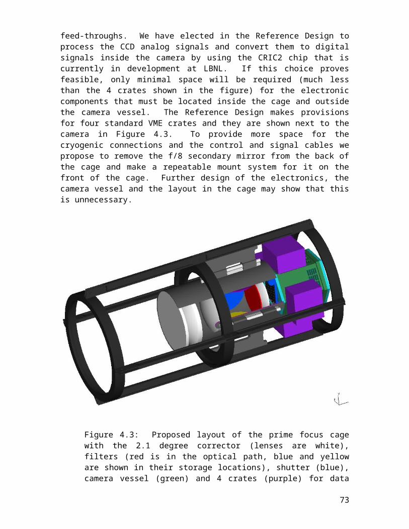
will be necessary to build our architecture.

On/Near Site: Operation Software (10-12 FTE months) Scheduling: (FTE-months: 4-6 month) tools for managing observing programs Archiving: (FTE-months: 4 months) ingest raw data into archive, producing level 0 dataQuality Assessment: (FTE-months: 2 months) automated measures of qualityQuick Alert Processing: (FTE-months: 0 months-CTIO/SCP collaboration) early detection of time domain phenomena

Archive-based Data Access: (12 to 15 FTE-months) Standard Collection Access: (FTE-months: 6+3/6 months) facilities for browsing and accessing data products.Archive Replication: (FTE-months: 3 months) processes for replicating large portions of the archive

Processing Pipelines: (47 to 51 FTE-months) Grid-based Pipeline Framework: (FTE-months: 9 months) infrastructure for executing pipelinesSimulation and System Verification: (FTE-months: 2+6 months) infrastructure for verifying correct data handling Single-Frame Calibration Pipeline: (FTE-months: 12 months) creation of calibrated images with astrometric solutions from a single scan in each of four colors, producing the level 1 dataCo-add Pipeline: (FTE-months: 12 months) cumulative combination of calibrated, single-frame images into four deep image databases of the sky, producing the level 2 dataSource Extraction Pipeline: (FTE-months: 12 months) creation of source catalog containing astrometry and photometry for all detected sources, producing the level 3 data

Science Analysis Pipelines: (31 FTE-months) Photometric Redshift Pipeline: (FTE-months: 3 months) provide four-color photometry and photometric redshifts for all detected galaxiesCluster-finding Pipeline: (FTE-months: 12 months) creation of a multi-frequency galaxy cluster catalog Weak Lensing Analysis Pipeline: (FTE-months: 12 months) creation of shear mapsSynoptic Analysis Pipeline: (FTE-months: 4 months + CTIO/SCP collaboration) time-domain-based analysis

Software Engineering: (9 FTE-months) Software Development Framework: (FTE-months: 6 months) documenting and managing the software processSoftware Repository: (FTE-months: 3 months) initialize and maintain

5.3 System and Software Development

5.3.1. Management of the Process

Because development will shared across the partnership (primarily UIUC and Fermilab), it is important to establish a working structure that makes leverages the distributed expertise effectively and efficiently. To this end, we will adopt a working group model for guiding the development of the system. Managing the overall effort will be a Project

73

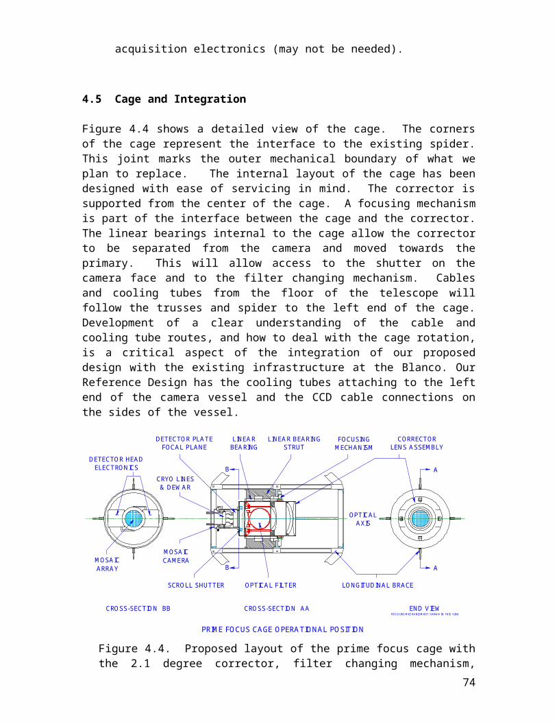
Manager specifically for the data management effort, who will lead the day-to-day operations. Another key player will the Project Scientist, who will be responsible for ensuring that the software meets the scientific requirements. Assisting these two will be two software working groups: the Data Management Steering Committee (DMSC) and the Computing Working Group (CWG). Membership need not be strictly controlled, but each should have representation from each of the partner sites at levels appropriate to their overall contribution to the project. The DMSC will be made up of leaders in the project from each site. They set the overall roadmap for data management, define the system requirements, and work out the high-level design. In contrast, the CWG is made up primarily of programmers and system specialists that will be involved in the detailed development of the various subsystems. The DMSC is expected to be most active in the early stages of development. The CWG will be formed later once the project is up and running; at that point, the main design activity will shift to the CWG with the DMSC playing more of an oversight role. Given the overall size of the project, it is likely that the two groups will share membership.

5.3.2 Software Engineering

The DMSC will develop the detailed requirements, from which they will develop a high-level design. From that, a set of work packages will be defined that define modules that make up the system. The work packages will then be assigned to appropriate people in the collaboration. The work package leaders will be responsible for developing a more detailed design for the module and overseeing its development. Actual development may involve multiple people across the different sites.

The DMSC will define a software review process that allows all partners to review and contribute to the design in an efficient way. The review process should be lightweight to ensure sufficiently rapid development. The review process will take place during the regular telecons of the working group (early on in the DMSC, later in the CWG).

5.3.3 Software Management

All code will be shared through CVS (or some other appropriate network-aware revision control system).

The DMSC will define a standard reference software environment used to develop the necessary software systems. Any software module must build and run in this reference environment. The development environment should be a close match to the expected production platforms and be reasonably simple to acquire on common developers' platforms.

The reference environment should not be so restrictive as to make it impractical to run the software except on a few specific computers (the exception, perhaps, being hardware interface software), nor so permissive that we support unused platforms. If the reference environment is simple to assemble, the code—particularly the pipeline software—will be more portable to other sites.

5.3.4 Data Release Strategy

74

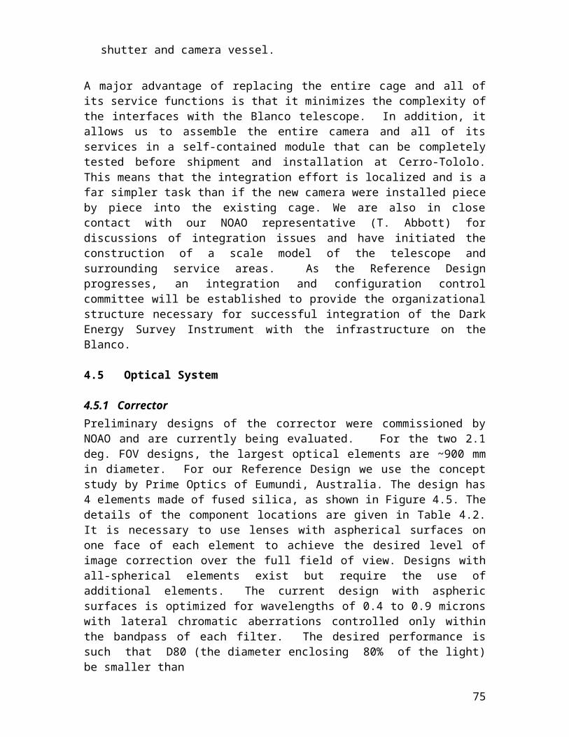
We will release raw and reduced single images, the level zero and level one data, after a proprietary period of 12 to 18 months from the night the data are acquired. This will occur in an automated fashion built into the public data access tools. Search tools will enable users to determine which data exist for a particular portion of the sky, listing acquisition dates, minimal quality information, and then allowing downloads of data that are older than the proprietary period.

The co-added database and object catalogs, the level two and three data, will be released in two stages. The first stage will occur at the end of the third year of the survey, when data from the initial, shallow survey over the entire SPT region will be released. The second stage will occur at the end of the sixth year (i.e. one year beyond the end of the survey), and these data will essentially serve as the final data release. Cluster catalogs, shear maps, photometric redshift estimates and other derived properties will be released upon publication of the results and at the discretion of the individual science teams.

5.4 The Role of Fermilab in Data Management

The Experimental Astrophysics Group and the Computing Division at Fermilab expect to make a substantial contribution of expertise and resources to this project. We expect to take the lead on several of the packages listed in section 5.2.2 and be major partners in more of them. This will be done in close collaboration with our colleagues as described in sections 5.2 and 5.3.

A major focus in the Fermilab effort in data management will be in creating the simulations necessary to provide a useful mock data challenge in 2007-2008. We expect this data set to be on order of the size of data we will obtain in our first year of operation. We expect to create the simulation data using Fermilab and grid resources, and to share these simulations with our partners at NCSA using grid storage resource management tools. These contributions will serve the dual purpose of 1) testing and verifying the data handling system from the end of the data acquisition system to the standard collection access methods, and 2) developing the grid-based pipeline framework and the archive replication processes. We could contribute our software repository expertise.

The Experimental Astrophysics Group expects to take the lead on the development of the co-add pipeline for the Processing Pipelines effort, based on current research in the co-addition of the five bandpass, 200-sq degree area of the SDSS Southern Survey. The Experimental Astrophysics Group also expects to take the lead on the development of the photometric redshift and cluster finding pipelines for the Science Analysis Pipelines, based on the research interests of EAG scientists. The processing code, and the science analysis pipelines in particular, are understood to be an collaborative efforts amongst the survey scientists, with the development process extending across institutional boundaries inside the survey.

5.5 Resources

5.5.1 Personnel

A current estimate of the labor requirements for this project can be gotten by summing the estimates for the individual packages listed in section 5.2.2. This yields 109-118 FTE months (9-10 FTE years). Much of this activity should take place during the camera

75

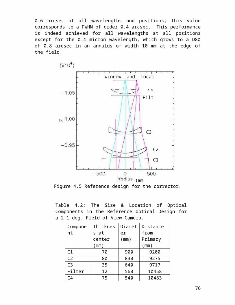
building (four yrs), and a lower level of effort will continue during the survey (five yrs). Given the early stage of this design, we believe it is prudent to double these estimates for a more realistic measure of the personnel required; in other words, we estimate needing approximately 4 FTEs per year over the five years.

NCSA and the UIUC administration has committed support for 1 FTE of a research programmer or astronomer to work on the Dark Energy Survey. Additional support will be sought from the National Science Foundation in a grant based at UIUC. In addition, there will be 6 FTE working on the design and implementation of a data management strategy for the Large Synoptic Survey Telescope. The Dark Energy Survey data management component will benefit from this parallel effort together with the existing NCSA experience in archiving, analyzing, visualizing and serving to the public of large astronomical datasets.

At Fermilab, we will need two computing professionals to support the grid management systems, maintain the storage systems, and develop grid-based processing infrastructure. This includes the integration of workflow management, virtual organization, and replica management tools. We will also need one full-time professional astronomer to lead development of data simulators and develop calibration and science analysis algorithms. We will also leverage the general participation of the EAG to support the science and the Computing group to support the hardware infrastructure. The computing professionals are expected to become necessary in stages during 2006 and 2007.

5.5.2 Hardware

NCSA will provide the hardware required for the data management task at the University of Illinois. This will be 100TB of disk space and 500TB of fast tape storage. CPU needs will be met on a range of machines through a minimal, guaranteed allocation of 10,000SU/yr and the option to propose for more resources as needed. These resources are routinely awarded cost-free within competitions. The emphasis on data management at NCSA for the long term will make it straightforward to access the CPU cycles needed for the data analysis. These resources and their maintenance will be provided by NCSA at no cost to the project.

At Fermilab, we estimate that we will need 20 TB by 2006 and 100 TB by 2008, initially to support system simulations and system verification but also, after observations begin, to photometric calibration efforts and quality assurance. This must be backed by a larger amount of Enstore tape space; by mid 2008, we expect to harness 500 TB of tape storage. We will need an order of 100 compute nodes by mid 2007 (either in the form of a group cluster or as a component of the Fermilab Farms system) to support simulation work. Later, this can be harnessed to augment general processing as well as detailed science analysis.

76

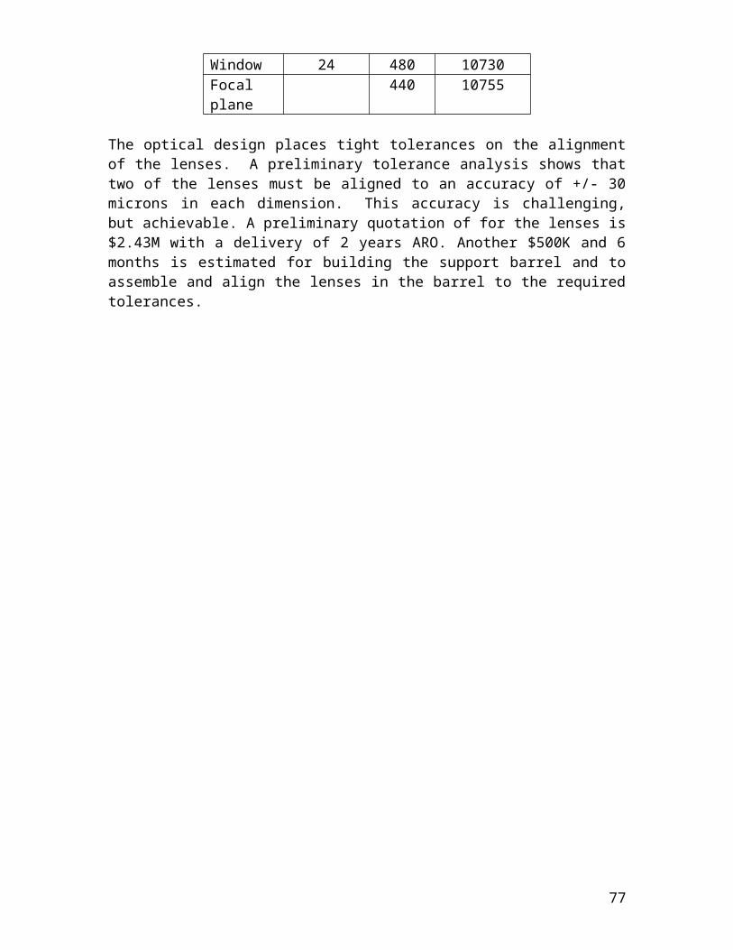
6. Project Management Structure and Near Term Goals

This chapter describes our project management structure that has allowed us to initiate the survey planning and conceptual design, and to prepare this proposal. It is a simple structure and it has served our needs. In November, we formed a Management Committee (MC) to guide our overall effort and in January, we formed the Dark Energy Camera team to design the Camera. More recently we formed the Science team and the Survey Strategy team. The remaining sections describe these teams and their immediate work plans. This Chapter also describes the prior, relevant experience of the participants.

6.1 Management Committee and its Functions

Each Management Committee (MC) member has specific responsibilities. The MC, with other participants, meets weekly by videoconference in order to track progress and identify critical items. About twenty scientists were engaged in the preparation of this proposal, the formulation of the science program, and the design of the camera. We expect the number will grow somewhat in the future since two institutions joined in March. The membership of the MC is as follows:

J. Annis Camera Project ScientistR. Brunner NCSA liaisonB. Flaugher Camera Project ManagerJ. Frieman Proposal Science Leader, University of Chicago liaison J. Mohr Data Management Project ScientistR. Plante Data Management Project ManagerJ. Peoples Management Committee ChairmanJ. Thaler Data Acquisition Project Manager W. Wester CCD and front-end electronics leader

The MC has at least one representative from each of the three founding institutions and we anticipate enlarging the MC to include at least one member from LBNL in the future. We will add a member from CTIO if our NOAO proposal is approved. Tim Abbott is currently serving as the CTIO/ NOAO technical contact for our NOAO proposal development and he participates in the weekly videoconferences. The MC is responsible for System Integration and all interfaces, hardware and software, among all institutions including CTIO and NOAO Data Products Division. The MC integrates the efforts of the Camera Team, Science Team and Survey Strategy Team through the participation of the team leaders in the MC decision process.

6.2 Dark Energy Camera Team

The Camera Team is made up of the Dark Energy Survey participants from Fermilab, the UIUC High Energy Group, and the LBNL Cosmology and Microsystems Groups. The Camera design effort is led by the Camera Project Manager, Brenna Flaugher, who coordinates the efforts of the PPD Support Departments and Technical Centers for the Camera Team, and directs the lead scientists who are responsible for the following areas:

77

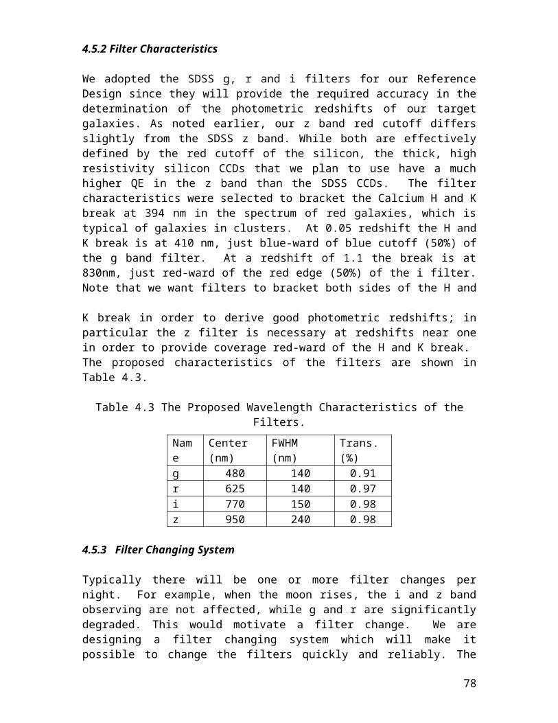
Camera Project Scientist J. AnnisOptical Design Coordinator S. KentCCD and electronics coordinator from FNAL W. WesterCCD and electronics coordinator from LBNL N. RoeData Acquisition System Manager J. Thaler

Typically one videoconference meeting per week is devoted to the Camera design and nearly all of the people working on the Camera participate. Members of the LBNL Cosmology and Microsystems groups have begun participating in these meetings and Natalie Roe coordinates their participation. William Wester coordinates the Fermilab Electrical Engineering Department participation in this effort as well. The LBNL groups have given the Camera Team considerable guidance on how to plan the acquisition of the CCDs and front-end electronics. Tim Abbott has also been a frequent participant in Camera design videoconferences. In that capacity he has provided critical information on the Blanco performance and the Cerro Tololo infrastructure. It has also received valuable engineering support from the PPD Electrical Support Department, Mechanical Support Department, and Technical Centers Department in the development of the Reference Design of the Dark Energy Camera. Brenna Flaugher is the primary contact for the Fermilab Engineering Departments and PPD Support Centers (such as SiDet) for the Camera. John Thaler of UIUC leads the design of the Data Acquisition System and its integration with Dark Energy Camera and CTIO infrastructure. His group has already begun evaluating Monsoon architecture in order to determine how to interface it to the two types of front-end electronics that the Camera team is evaluating. The UIUC group plans to acquire sufficient Monsoon hardware to build a test set up in the near future. With the exception of an Optical Designer, the current Camera Team, including the FNAL engineering support, has the skills and size to complete the Camera design and initiate the CCD and front-end electronics development and testing program.

6.3 Science Team

The Science Team is responsible for the development of the scientific program and science goals of the proposal. While the Science team is open to all participants, Frieman, Mohr and Annis have led the development of the proposal science with significant contributions from Aldering, Hu, Lin, Kent, Perlmutter, Sheldon, Smith, Suntzeff, Thaler, and Wechsler.

In the near term, this team will develop a better understanding of the requirements that the science goals impose on the science software and the survey calibrations. They will also clarify the synergies between the Dark Energy Survey and the future more ambitious projects such as LSST and JDEM, as mentioned in Chapter 7.

6.4 Survey Strategy Team

The Survey Strategy team is responsible for developing the observing plan and assuring that it will meet the science goals. The team includes participation from B. Flaugher, J. Frieman, J. Mohr, D. Tucker and W. Wester and it is led by J. Annis and H. Lin. This effort includes the photometric calibration, and will expand to include the simulations that are relevant to observing strategy and the mock data challenge. The planning for the mock data challenge will begin in April and it will be done jointly with the Data Management team. The Survey Strategy team will include liaisons from the Data

78

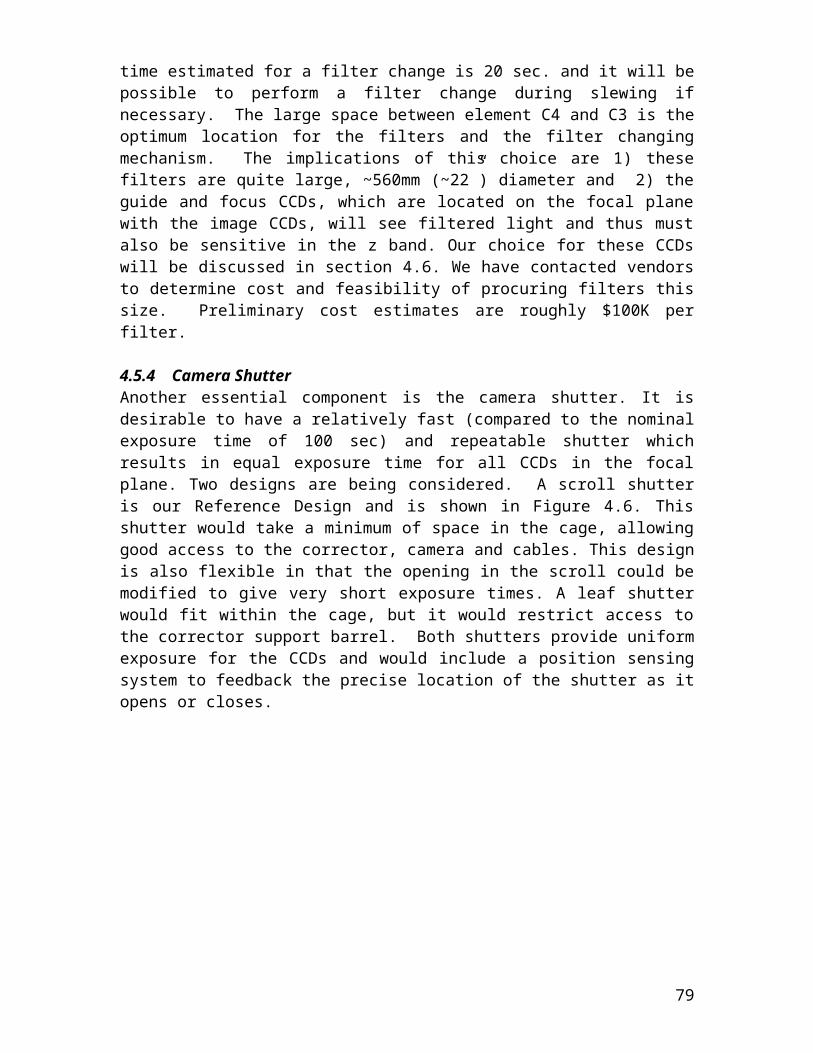
Management team, the Science team, and the Dark Energy Camera team who will serve as the points of contact.

6.5 Data Management Team

This team is lead by the Data Management Project Scientist and the Data Management Project Manager. They are responsible for defining the Data Management framework and coordinating the work of the Data Management team. They will continue to define the Data Management tasks, including the computing framework, data processing and archiving. Plante and Mohr lead this effort, with contributions from Annis and Frieman. The Data Management team will also establish the computing framework for the simulations so that the code and results are properly archived, thereby making them available to the entire collaboration. Additional details of the Data Management organization are presented in section 5.3.1 of Chapter 5.

6.6 Relevant, Prior Experience of the Dark Energy Survey Collaboration

6.6.1 Camera Construction

While the construction of a wide-field camera will be a new challenge for Fermilab, the Dark Energy Camera team includes scientists and engineers who have built state of the art silicon vertex detectors. Vertex detectors use many of the technologies and technical skills that are directly relevant for the construction of wide-field cameras. The accurate placement of sensors in a silicon vertex detector has important similarities with the accurate placement of CCDs on a focal plane and SiDet has superb facilities to build a focal plane. The Fermilab group at SiDet, which has extensive experience in wire bonding, is evaluating whether the techniques and facilities used at SiDet for wire bonding front-end electronics to the silicon vertex sensors can also be adapted to bonding the camera front-end electronics onto the CCDs. In addition, CCD sensors share a common technology base with the silicon vertex detectors sensors. As noted earlier, the Fermilab and LBNL groups are exploring the use of the thick, high resistivity CCDs in the Dark Energy Camera. The LBNL groups have developed state of the art CCDs of this type, including their front-end electronics, for applications in astronomy over the past five years. Devices very similar to the devices specified in the Camera Reference Design have already been successfully deployed in telescopes at Kitt Peak. However, the use of the 2K x 4K LBNL CCDs in our proposed camera will require the creation and evaluation of a new mask for the production vendors. The Fermilab and LBNL members of the Camera team have developed a preliminary plan to do this. In the past, Fermilab and LBNL have worked closely to develop several generations of the SVX chips and vertex detectors for the current CDF and DZero experiments and thus it is natural for the Fermilab and LBNL participants to explore a similar partnership for the Dark Energy Camera.

6.6.2 Data Management

The University of Illinois Astronomy group has extensive experience in analyzing and archiving large optical and radio astronomy datasets. NCSA provides basic data management for all users of NCSA computing facilities across a variety of fields of science and engineering. Plante, as part of the NCSA Radio Astronomy Imaging group, has led the development and operation of the NCSA Digital Image Library, the BIMA

79

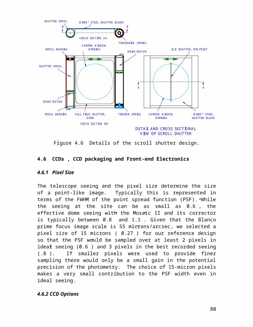
Data Archive and the BIMA Image Library. The astronomy group also has extensive experience in distributed (cross-institution) software development. In the early 1990s, NCSA was a partner in the development of the Miriad software system for radio interferometers. It was a founding member of the AIPS++ consortium, and it is currently a collaborator in the CARMA (Combined Array for Research in Millimeter Astronomy) Software Development project. Along with Fermilab, it is a collaborating institution in the National Virtual Observatory (NVO).

The Fermilab participants from the Experimental Astrophysics Group (EAG) have gained extensive experience with data management of large surveys through their fourteen-year participation in the SDSS. In particular, they contributed to coding and debugging the pipelines for the SDSS, they operate the data reduction center for the SDSS, and they are responsible for a major part of performing data quality assurance on the processed SDSS data. The EAG was very active in the creation of the SDSS archive and it manages and operates it.

It is from this extensive experience in data management and distributed software development that our data management plan has been drawn and gives us confidence that we can meet the DES requirements for data management and place this archive in the NVO.

6.6.3 Data Analysis and Interpretation

The members of the Fermilab Theoretical Astrophysics Group and the University of Chicago participants have made important contributions to the interpretation of the data from large surveys in the framework of the standard model of cosmology. The Fermilab Theoretical Astrophysics group was the first group at a DOE National Laboratory to specifically set out to explore the connection between the early universe and particle physics. Both groups have made important contributions to the interpretation of large-scale structure (galaxy), cluster counts, and weak lensing, and all of the analysis techniques that will be used to achieve the scientific goals of the Dark Energy Survey. Moreover, with members of the EAG, they have been active in applying these techniques to the analysis of SDSS data. The EAG participants also have experience in the analysis of wide-field multi-color surveys such as SDSS and CNOC2. The Fermilab particle physicists plan to contribute to the science analyses.

University of Illinois scientists have focused on cosmology, structure formation, quasars and galaxy formation using data from X-ray satellites, optical observations, interferometric SZE observations and large scale, near-infrared surveys carried out by 2MASS and at Kitt Peak National Observatory using the FLAMINGOS camera. In addition, one Illinois scientist is involved in the data analysis and interpretation of the DPOSS optical plate survey and the QUEST2 time domain CCD survey.

The LBNL Cosmology Group established a strong reputation for developing the successful observing strategies that allowed them to discover large numbers of supernova and follow their light curves. Their subsequent analysis of this data helped to establish some of the basic parameters of the concordance model of cosmology. The CTIO Dark Energy Survey participants are members of an independent group that developed similar observation strategies and analysis techniques for discovering and understanding supernovae. That group has achieved similar results of great importance. The two

80

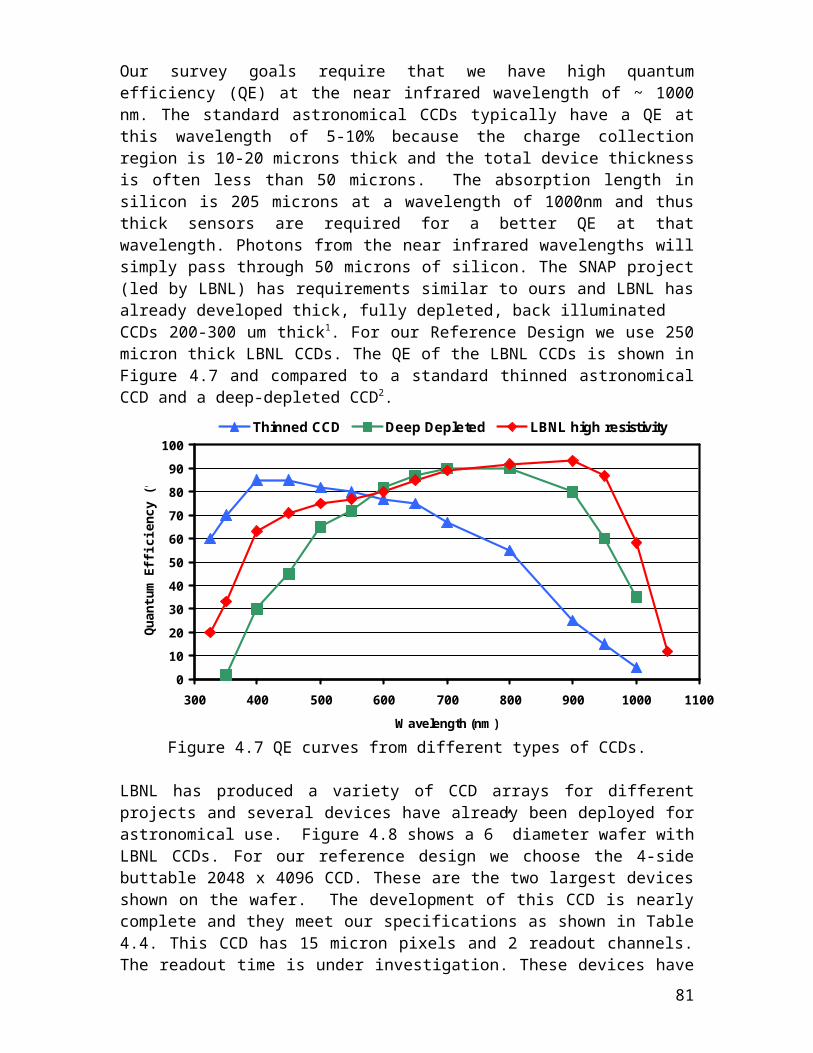
competing teams independently discovered the accelerating universe, perhaps the most profound discovery in cosmology in the past two decades.

6.7 Near Term Goals We have set the following goals for the four teams for the next four months:

Develop a complete proposal for the Dark Energy Survey so that it can be reviewed by an independent group in early June and after revision submitted to NOAO in August;

Augment the optical design effort at Fermilab with a consultant to complete the optical design of the corrector and assure that it meets the science requirements and is cost effective;

Initiate the CCD and front-end electronics development and testing program;

Bring the data management framework to the next level of functionality to enable the start of simulations.

Bring the Reference Design to a complete preliminary engineering design;

In August, we must submit the proposal to NOAO to build and commission the Dark Energy Camera if we are to participate in the competition. We also plan to fill in the details of the data management system and the relationship of NCSA to the computation efforts at the other participating sites. At that time, we will also be in a position to define the nature of the partnership with NOAO-CTIO (telescope and observing) and NOAO-Tucson (data archiving). We will prepare a formal project management plan as part of the proposal to NOAO. We are persuaded that our current management structure will serve quite well at least until we begin to build hardware and software systems.

81

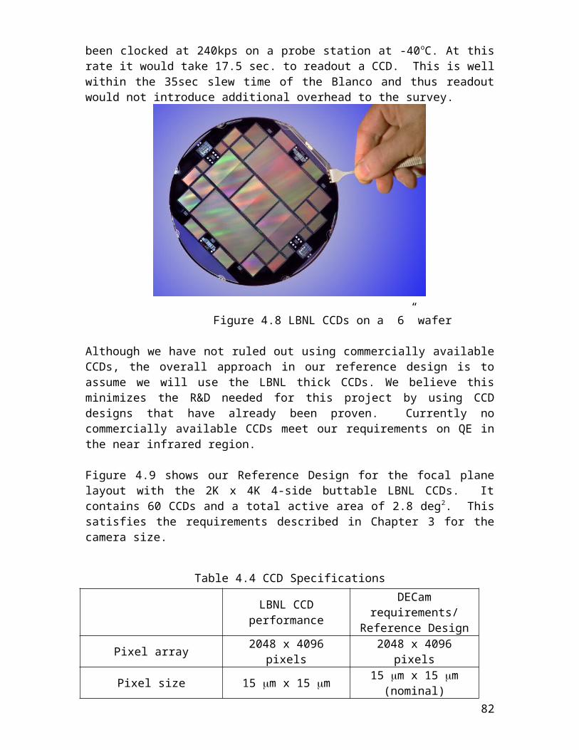
7. The Relationship of the Dark Energy Survey to other Astrophysics Projects

This chapter describes the commitments of the Dark Energy Project participants to other astrophysics projects and it also describes the temporal relationship of these projects to the Dark Energy Project within each institution.

7.1 Fermilab Projects

Fermilab scientists and staff are engaged in both the SDSS and SNAP projects. The Fermilab EAG has had a major involvement in the SDSS over the past fourteen years. The initial five-year observation phase of the SDSS will end July 1, 2005. The SDSS consortium has developed a plan for a three-year extension and is actively seeking funds for the extension. While some Fermilab scientists will actively participate in the extension, the Fermilab astronomers from the EAG who plan to participate in the DES will reduce the level of their contributions to the SDSS infrastructure after July 2005. Since the survey will have been in operation for five years and its operation is mature the demands on the Fermilab participants can be reduced. In addition, two Fermilab scientists recently joined the SDSS supernova effort and are active participants in planning and leading the SDSS supernova campaign. Their participation in the SDSS will help to share the load of infrastructure work with the EAG astronomers who plan to continue to work actively on the SDSS extension. The EAG proposes to support the data processing of the SDSS imaging data and to manage the full SDSS archive during the extension. The SDSS will either end in July 2008, if all of the funding for the extension is secured, and if the funding is not secured it will end earlier. When that happens, the computer professionals and the astronomers in the EAG could contribute to both the pre-launch phases of SNAP and the operations phase of the Dark Energy Survey. The EAG computer professionals have the ability to provide support for simulations, observations, data processing, data analysis and archiving once the SDSS ends. Nevertheless, the Dark Energy Collaboration does not plan to make large demands on the EAG support team since the data management and data distribution effort will be led by and primarily supported by the University of Illinois.

The EAG members have been joined by several Fermilab particle physicists to form the Fermilab SNAP group. All are engaged in contributing to the SNAP collaboration development of the science case for SNAP. The wide area survey part of SNAP, which includes both weak lensing, and cluster counts, is of particular interest to the Fermilab DES participants who are engaged in SNAP. They believe that this effort will speed the development of DES simulations and refine the DES observing strategy, since the Joint Dark Energy Mission (SNAP) will probably not be launched until after 2013, the Dark Energy Survey will fit nicely in the temporal gap between the end of the SDSS and the start of JDEM.

7.2 University of Illinois Projectsionship of the Dark Energy Survey to Astrophysical Projects at the Other Institutions.One of the University of Illinois astronomers (J. Mohr) is a member of the South Pole Telescope Collaboration, and all of the University of Illinois members are participating in LSST. In particular, the University of Illinois, in partnership with the NCSA, plans to be a major data processing and archiving center for LSST. As noted earlier, this relationship

82

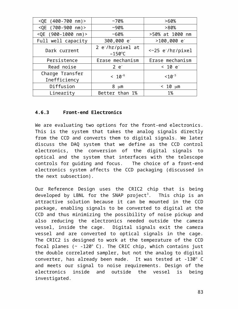
will strengthen the Dark Energy Survey Collaboration. The needs of the two projects and their schedules nicely match the availability and interests of the scientists and technical staff at the University of Illinois.

7.3 University of Chicago Projects

The University of Chicago members of the Dark Energy Collaboration are active in several astrophysical projects. Josh Frieman, who is the DES liaison with the University of Chicago Astronomy and Astrophysics Department, is a member of the SDSS, and coordinated the development of its spectroscopic pipeline software. He is co-chair of the SDSS Large Scale Structure Working Group and is active in the analysis of large-scale structure and weak lensing data. In addition, he serves on the SDSS Collaboration Council and is the Fermilab representative on the SNAP Institutional Board. He has also been engaged in unrelated observation projects at CTIO in the past. John Carlstrom is the PI of the South Pole Telescope Project and the leader of the SPT collaboration, which includes the UC Berkeley /LBNL Cosmic Microwave Background Group. He will be the primary contact between the SPT Collaboration and the Dark Energy Collaboration. In this capacity, he will help to define the procedures for analyzing the relevant data sets created by the two surveys.

7.4 CTIO Projects

The CTIO participants are actively engaged in the ESSENCE Project, which will detect and follow up on ~200 supernovae that will be observed with the Blanco telescope. The ESSENCE Project is expected to be complete in the next 3 years. They are also pursuing the observation of nearby supernovae, since these observations will tie down the Hubble diagram at zero redshift. They are also engaged in the use of the Monsoon system with the NEWFIRM Camera. These efforts will help the Dark Energy Survey.

7.5 LBNL Projects

The LBNL Cosmology Group is engaged in three projects: the Supernova Cosmology Project (SCP), the Nearby Supernova Factory (SNF), and SNAP. The Supernova teams are working with the CFHT Supernova Legacy Survey using Megacam. The goals of this observing campaign are similar to the ESSENCE Project. The Nearby Supernova Factory will discover ~300 nearby supernovae with the NEAT telescopes and follow them up with new instruments on the Hawaii 2.2-meter telescope. Both the SNF and the CFHT Supernova Legacy Survey are expected to be completed in the next 4 years. LBNL is the lead institution for the proposed SNAP mission.

83

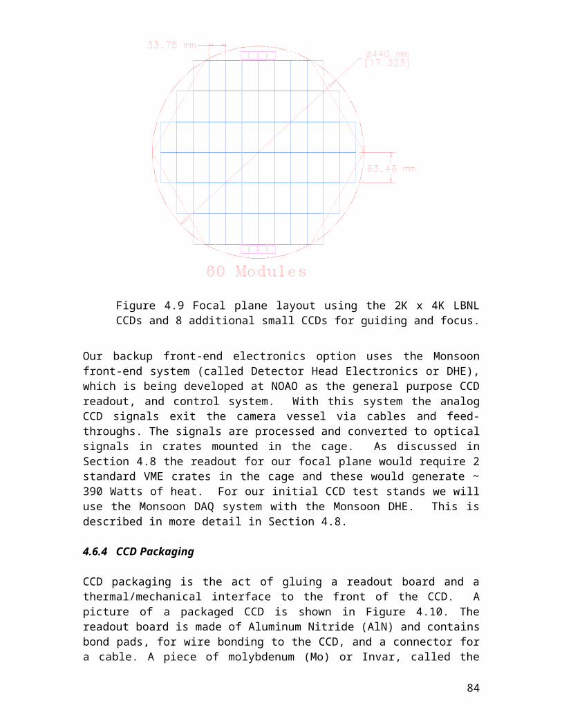
8. Conclusions

The purpose of this proposal is to request permission for the Fermilab team to join the Dark Energy Survey collaboration so that it can contribute to the NOAO proposal for the Dark Energy Survey and to participate in the collaboration program of technical design and science analyses. The primary goal of our scientific program is to obtain a more precise determination of the equation of state of the Universe, w, through four independent, complementary measurements. While we intend to focus our efforts on dark energy and dark matter, the survey data will also provide the scientific community with data that will be relevant to a broad range of current problems in astrophysics and cosmology. We believe it presents a superb scientific program and if it is carried out it will have an important impact on the science at the intersection of particle physics, astrophysics, and cosmology. This proposal describes our preliminary plan for building the camera and the software systems that will be needed to support the survey science program. We are confident that we can win the competition if the Laboratory supports the Fermilab team at the requested level and with that support we are convinced that we can carry out this program.

We believe the Dark Energy Survey fits well in the context of the long term plans of the field. The Connecting Quarks with the Cosmos Report recommended that ground- and space-based wide-field telescopes with Gigapixel-scale cameras be pursued to address the dark energy question. The Report highlighted two major complementary projects that have been proposed with primary goals that include probing the dark energy. The Supernova/Acceleration Probe (SNAP) is a satellite concept for the NASA-DOE Joint Dark Energy Mission that will include a deep z>1 supernova survey and a wide-area weak lensing survey. The Large Synoptic Survey Telescope (LSST) is a proposed 8-meter telescope with a wide-field imager that will carry out multiple scans over ~1/2 of the sky to study cosmology, particularly via weak lensing and transient astronomical phenomena. These projects aim to achieve exquisite precision on cosmological parameters using complementary techniques and in particular go deep enough to offer the possibility of constraining the time evolution of the dark energy, provided systematic errors can be controlled at a fine level. Designed as ‘ultimate’ experiments, they involve significant technological development and necessarily long lead times; both projects aim to begin science operations on the order of a decade from now.

The Dark Energy Survey, by contrast, is more modest in scale, cost, and science goals, but it will deliver excellent dark energy science on a shorter timescale. It will serve as both a scientific and technical precursor to these major projects and therefore constitutes the logical next step for this field. The Dark Energy Survey will enable us to learn much about the dark energy and about the limitations and relative advantages of the different techniques for probing it, knowledge that will be useful for the larger projects to follow. Many participants in the Dark Energy Survey are participating in the planning and design of LSST and SNAP. They are also participants in experiments that are providing results now. The Dark Energy Survey can be mounted soon after the current experiments finish and the observing phase will almost be completed just as the more ambitious surveys reach the observation stage. For these reasons we believe that the Dark Energy Survey fits nicely between the two sets of surveys and that it will provide a substantial advance in the precision of Dark Energy relative to the current surveys. Moreover, as a precursor to LSST and SNAP we anticipate substantial cross-fertilization and knowledge transfer that will be useful for all the projects.

84

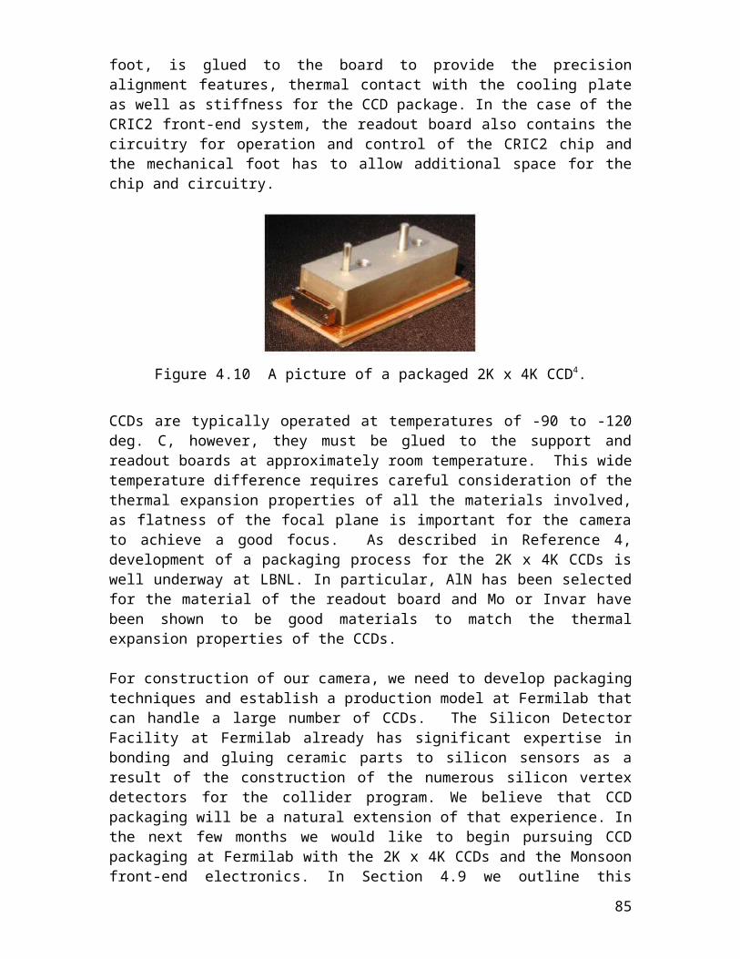
We have assembled a strong, experienced team to reach our scientific and technical goals. We have come a long way since our first collaboration meeting at Fermilab in early December. At that time our collaboration had fewer participating institutions and there were gaps in our technical capabilities that would have hampered our ability to mount our survey in a timely way. Our new collaborators bring technical capabilities that more than fill those gaps. Moreover, their participation has strengthened and enriched our scientific program. The role of Fermilab is central to the collaboration, and if we are to progress quickly, which is essential if we are to win the competition, we must do the following during the remainder of this calendar year:

Order mechanical and electrical CCDs for packaging studies;

Design and build a CCD testing station;

Design a new wafer mask with four 2K x 4K CCDs and place the minimal order with the foundry (24 wafers);

Contract an optical designer and develop a more cost effective design;

Build a realistic model of the Blanco for integration;

Complete the preparation of the NOAO proposal that is due Aug. 15th.

In order to complete these tasks quickly and effectively the collaboration makes the following request of the Laboratory:

Labor: the Fermilab group needs the full time equivalents of 1 electrical engineer, 2 mechanical engineers, 1 mechanical technician and 1 design/drafter and 30% of an electrical technician for the next three quarters.

Budget: In order to obtain the needed materials and services the Fermilab group needs a cash budget of $100K and $219K in the last two quarters of FY04 and $512K in the 1st quarter of FY05 respectively.

We have described these requests in much greater detail in Chapter 4 of this proposal.

We realize that this is a significant request, but we must take forceful steps in the beginning if we are to succeed. By moving forward aggressively during the remainder of this calendar year we can develop a cost-effective design that is consistent with our science goals. By the standards of today’s, or even yesterday’s high-energy physics proposals, this project requires a modest cash outlay. In order to assure that the burden of the cash budget will not fall solely on Fermilab and DOE we will work with our partner institutions to find ways to share the cash burden.

The science opportunities of the Dark Energy Survey are important, timely and directly relevant to particle physics and astrophysics. Our collaboration has the capabilities needed to build the camera, manage the data, and carry out the science analysis, and we request the opportunity to move forward on this significant and exciting program.

85