a preliminary fish survey of the estuaries on the

82

http://dx.doi.org/10.4314/wsa.v42i1.10Available on website http://www.wrc.org.zaISSN 1816-7950 (On-line) = Water SA Vol. 42 No. 1 January 2016Published under a Creative Commons Attribution Licence

A preliminary fish survey of the estuaries on the southeast coast of South Africa, Kayser’s Beach – Kei Mouth: a comparative study

NC James1* and TD Harrison2,1

1South African Institute for Aquatic Biodiversity, Private Bag 1015, Grahamstown, 6140, South Africa2Marine Division, Department of the Environment (Northern Ireland), 17 Antrim Rd, Tonagh, Lisburn, BT28 3AL, Northern Ireland

ABSTRACTA basic ichthyofaunal and physico-chemical survey of estuaries on the southeast coast of South Africa from Kayser’s Beach to Kei Mouth was undertaken during September and October 1996. Twenty-eight (28) estuaries have been identified along this stretch of coastline, and these were grouped into three types: small (<10 ha) predominantly closed estuaries, moderate to large (> 10 ha) predominantly closed estuaries, and predominantly open estuaries. Multivariate analyses revealed significant differences between estuarine types both in terms of their physico-chemical characteristics and fish communities. These features were consistent with those reported in other parts of the south and southeast coast. Overall, predominantly closed estuaries had a lower species diversity than predominantly open estuaries and smaller systems had a lower species diversity than moderate to large systems. Although differences were observed between estuarine types, most systems provided important habitat for a number of estuarine-dependent marine species as well as resident species, which were often recorded in high numbers. Many of these species were also endemic, which further emphasises the importance of these estuaries in maintaining ichthyofaunal diversity in the region. This survey represents one of the few fish surveys undertaken along this little-studied section of coastline.

Keywords: ichthyofauna, estuarine survey, fish habitat, southeast coast

* To whom all correspondence should be addressed.e-mail: [email protected]: 17 February 2015; accepted in revised form 18 November 2015

INTRODUCTION

Warm-temperate estuaries constitute important nursery areas for a number of estuarine-associated fish species (e.g. Potter and Hyndes, 1999; James et al., 2007a). Despite the impor-tance of these systems as nursery areas, habitat degradation, hydrological manipulations, overexploitation and pollution increasingly threaten these systems (Whitfield and Cowley, 2010). In order to understand change in estuaries and maintain their ecological function, basic information is needed on fish assemblages. This information is often lacking, particularly for estuaries on the southeast coast of South Africa, around East London. Although studies have been carried out on the biology of the Nahoon (Steinke, 1986; Campbell et al., 2001; Bursey and Wooldridge, 2002; 2003; Sale, 2007; Geldenhuys, 2013), Nyara (Perisinotto et al., 2000, Walker et al., 2001), Goda (Vumazonke et al., 2008) and Haga Haga (Whitfield, 1992) estuaries, no information exists on fish biodiversity for the majority of systems along this coastline. There have only been two studies conducted which have focused of fish: one on recruitment of ichthyoplankton into the Haga Haga Estuary (Whitfield, 1992) and one on the feeding dynamics of four species in the Goda Estuary (Vumazonke et al., 2008). As part of a national assess-ment of South African estuaries, a fish survey was undertaken along the southeast coastline between Kayser’s Beach and Kei Mouth; basic physico-chemical variables, fish community data and a comparative analysis are provided.

STUDY AREA

The Eastern Cape region falls within a transitional area of climatic zones and experiences relatively mild summers and

winters (Kopke, 1988; Stone et al., 1998). Seasonality of rainfall is less pronounced than in other parts of the country (Stone et al., 1998) and, although rainfall may occur at any time of the year, it usually displays an autumn/spring bimodal pattern with peak rainfall in spring (Kopke, 1988). The coastline is influ-enced by the south-flowing Agulhas Current (Shannon, 1989; Heydorn, 1991). Being tropical in origin, the waters of this current are relatively warm; however, as it flows south it tends to cool with inshore water temperatures along the Eastern Cape coast varying between 14 and 20°C (Day, 1981). The section of coastline between Kayser’s Beach and Kei Mouth extends some 68 km and is intersected by 31 river outlets (Fig. 1). The city of East London is the major metropolitan area situated on this coast.

MATERIALS AND METHODS

The estuaries between Kayser’s Beach and Kei Mouth were sampled between September and October 1996. Each system was sampled once and took 1–3 days to survey, depending on the size of the system.

Physico-chemical

During each survey, selected physico-chemical parameters were measured at various sites within each system ranging from the mouth area (Site 1) upstream; the number of sites varied depending on the size of each system. Water depth and trans-parency were measured using a 20 cm diameter Secchi disc attached to a weighted shot line graduated at 10 cm intervals. Temperature (°C), salinity (psu), pH, dissolved oxygen (mg∙L−1), and turbidity (NTU) were measured using a Horiba U-10 Water Quality Checker. Where water depth permitted (usually >0.5 m), both surface and bottom waters were measured. The mouth state of each system at the time of sampling was also noted.

http://dx.doi.org/10.4314/wsa.v42i1.10

http://www.wrc.org.za

mailto:n.james%40saiab.ac.za?subject=

83


Figure 1Coastal outlets between Kayser’s Beach and Kei Mouth on the southeast coast of South Africa

Ichthyofauna

The ichthyofauna of each estuary was sampled using a 30 m long x 1.7 m deep x 15 mm bar mesh seine net fitted with a 5 mm bar mesh purse, and a fleet of multi-mesh gill nets. The gill nets were either 10 m or 20 m in length and 1.7 m in depth and consisted of three equal sections of 45 mm, 75 mm and 100 mm stretch meshes. Seine netting was carried out during daylight hours in shallow (< 1.5 m deep), unobstructed areas with gently sloping banks. Fish caught were identified and measured to the nearest millimetre standard length (SL) before being released. Where large catches of a species were made, a sub-sample was kept and returned to the laboratory where the fish were identified, measured and weighed to the nearest 1.0 g; specimens that could not be identified in the field were also kept and processed in the laboratory. All fishes were identified by reference to Smith and Heemstra (1991) and Skelton (1993); taxonomic identities of certain species were adjusted using information provided in Heemstra and Heemstra (2004). The total fish species composition, by number and mass, was calcu-lated for each system. The relative biomass contribution of each species was calculated using actual recorded masses as well as masses derived from length–mass relationships provided in Harrison (2001).

Estuary classification

Estuaries were divided into two main groups on the basis of predominant mouth condition, according to the classification given in Harrison and Whitfield (2006). The two main groups

were predominantly open estuaries and predominantly closed estuaries. Predominantly closed estuaries were further sub-divided into two groups based on surface area: small closed estuaries with a surface area below 10 ha and moderate to large closed estuaries with a surface area above 10 ha.

Multivariate analyses

Data were analysed using the Plymouth Routines in Multivariate Ecological Research (PRIMER) package (version 6.0). A principal component analysis (PCA) was undertaken on the overall mean (surface and bottom) values of the physico-chemical variables recorded in each system. Each parameter was first examined for normality; only turbidity required log-transformation (ln[1 + x]). The data were also examined for any inter-correlations (Pearson r); pH exhibited significant correla-tions (p < 0.05) with both dissolved oxygen and temperature and was omitted from the analysis. Although salinity and depth also showed a significant correlation, these parameters were retained. A PCA was performed based on the following normalised parameters: depth, temperature, salinity, dissolved oxygen, and turbidity. An analysis of similarities (ANOSIM) was also undertaken (using the normalised Euclidean distance similarity measure) to test for significant differences between estuarine types. Estuaries sampled during the latter part of the survey (Kwenxura – Cwili) were sampled following heavy rainfall in their catchments, which led to breaching of the mouths of closed estuaries, reduced salinities in some cases, and elevated turbidities. These estuaries were excluded from the ANOSIM test.



84


Fish catch data were subject to non-metric multidimen-sional scaling (MDS) ordination. Specimens not identified to species level (e.g. Mugilidae) as well as exotic species (e.g. Micropterus spp.) were excluded from the analysis. Abundance and biomass data were first standardised and then square-root transformed before calculating a Bray-Curtis similarity matrix. Standardisation removed the effect of variable sampling while transformation scales down the importance of dominant spe-cies (Field et al., 1982; Clarke and Warwick, 2001). An ANOSIM test was applied to both the abundance and biomass data to examine differences in fish communities between estuary types. Obvious outliers identified in the MDS plots were omitted from the ANOSIM test. A similarity percentages analyses (SIMPER) was also undertaken to identify species that characterise estuary types as well as those that discriminate between estuary types.

RESULTS

A total of 31 systems were sampled between Kayser’s Beach and Kei Mouth. Three systems, (Imtwendwe, Mvubukazi, and Ngqenga) comprised small coastal streams and were not considered further. Of the remaining systems, 5 were pre-dominantly open estuaries and 23 were predominantly closed estuaries – 13 estuaries were small closed systems and 10 were moderate to large closed estuaries.

Physico-chemical

Small predominantly closed estuaries

Of the 13 small predominantly closed estuaries, 7 were open to the sea at the time of sampling. Systems such as the Haga-Haga, Mtendwe, and Cwili had all breached as a result of high river flows following heavy rainfall in their catchments. The outlets in the other systems appeared to have formed as a result of the lowering of the barrier at the mouth by wave action. All estuar-ies were relatively shallow, with average water depths generally not exceeding 1.0 m (Table 1). Water temperatures averaged between 17.8°C (Blind) and 24.6°C (Cunge). Mean salinities ranged from almost fresh (0.3) recorded in the Mtendwe to 27.7 recorded in the Hlozi. Salinities were fairly uniform throughout most of the systems with no clear horizontal or vertical gradi-ents. Only the Hlozi and Hlaze estuaries exhibited a horizontal decrease in salinity of more than 1.0, while a marked verti-cal salinity gradient was only evident in the Cunge and Cwili estuaries. Average dissolved oxygen values ranged between 3.4 mg∙L−1 (Mtendwe) and 11.8 mg∙L−1 (Shelbertsstroom), with most systems exceeding 7.0 mg∙L−1. Mean turbidity values ranged from 3.5 NTU (Hlozi and Hlaze) to 36.2 NTU (Cwili); relatively high (>33 NTU) average turbidities were recorded in the Haga-Haga, Mtendwe and Cwili systems, a result of heavy rainfall in their catchments. Average pH values (7.5–8.1) in all estuaries were characteristic of seawater (Table 1). Physico-chemical parameters by site are given in Table A1 (Appendix 1).

Moderate to large predominantly closed estuaries

Three (Kwenxura, Nyara, and Morgan) of the ten moderate to large predominantly closed estuaries were open to the sea at the time of this survey; high river flows following heavy rainfall in their catchments resulted in these estuaries breaching. Apart from those estuaries that had recently breached, mean water depths generally exceeded 1.0 m (Table 1). Water temperatures averaged between 19.0°C (Nyara) and 23.8°C (Cintsa). Water

temperatures generally increased from the lower to the upper reaches of the estuaries; there was very little vertical tempera-ture stratification. Mean salinities ranged from 8.6 (Morgan) to 33.7 (Ncera) with values generally exceeding 21.0. Salinities were fairly uniform in most systems with no clear horizontal or vertical gradients. A pronounced axial salinity gradient, however, was present in the Nyara and Morgan estuaries with salinities decreasing upstream from the mouth; this is a result of high freshwater inflow following rainfall in the catchment. Mean dissolved oxygen values ranged from 3.5 mg∙L−1 (Nyara) to 8.4 mg∙L−1 (Morgan) with most values exceeding 5.0 mg∙L−1.

TABLE 1Mean physico-chemical parameters measured in estuaries between Kayser’s Beach and Kei Mouth on the southeast

coast of South Africa, September-October 1996

Estuary MouthDepth

(m)Temp.

(°C)Salinity

Diss. oxygen (mg∙L−1)

Turbid. (NTU)

pH

Small closed estuaries

Shelbertsstroom Closed 1 19.8 6.8 11.8 6.6 8.1

Lilyvale Closed 0.8 21 17.6 9.4 21.6 8

Ross’ Creek Closed 0.6 18.9 6.6 6.6 20 7.8

Mlele Closed 1.1 19.8 15.3 7.5 16 7.8

Mcantsi Open 1 23 14.1 7 7 7.9

Hlozi Closed 1.3 20.2 27.7 7.3 3.5 7.7

Hickmans Closed 1.6 22 18.8 6.4 5.2 7.5

Blind Open 0.2 17.8 0.8 8.9 19 7.9

Hlaze Open 0.5 21.5 23 9.3 3.5 8

Cunge Closed 0.5 24.6 18.6 7.4 4 7.7

Haga-Haga Open 0.5 21.3 25.8 8 33.7 7.7

Mtendwe Open 0.8 21.8 0.3 3.4 33.5 7.8

Cwili Open 0.8 20.6 16.6 7.7 36.2 7.8

Moderate to large closed estuaries

Ncera Closed 1.2 20.5 33.7 7.7 2.4 7.9

Gxulu Closed 1.4 22.1 29.6 6.4 3.9 7.8

Goda Closed 2 21 32.6 6.1 6.2 7.8

Qinira Closed 1.7 21.5 28 6.4 4.8 7.7

Bulura Closed 1.2 22.9 29.2 7.5 4 7.9

Cintsa Closed 1.4 23.8 31.1 5.5 3.4 7.5

Cefane Closed 0.9 23.5 28.9 5 7.1 7.6

Kwenxura Open 0.8 19.7 29.1 7 34.6 7.9

Nyara Open 0.6 19 21.8 3.5 73.3 7.9

Morgan Open 0.6 22 8.6 8.4 103.7 7.6

Permanently open estuaries

Buffalo Open 3.4 18.2 31.2 7.8 12.8 7.9

Nahoon Open 2.3 19.4 32.6 8.4 5.9 7.9

Gqunube Open 1.7 20 32.8 6.8 17.4 7.9

Kwelera Open 1.6 21 32.1 6.8 18.8 7.7

Quko Open 1.5 20.7 10.4 8.3 265 7.7



85


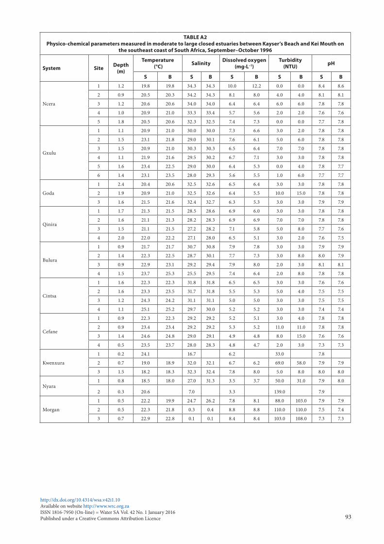
Most of the estuaries were fairly clear, with average turbidi-ties not exceeding 10 NTU. Only the Kwenxura, Nyara and Morgan estuaries were turbid, averaging between 34.6 and 103.7 NTU; this is a result of turbid freshwater inflow following rains in their catchments. Mean pH values ranged from 7.5 to 7.9 (Table 1). Physico-chemical parameters by site are given in Table A2 (Appendix 1).

Predominantly open estuaries

Mean water depths recorded in the five predominantly open estuaries ranged from 3.4 m (Buffalo) to 1.5 m (Quko) (Table 1). Water temperatures averaged between 18.2°C (Buffalo) and 21.0°C (Kwelera). Generally, water temperatures increased upstream from the mouth in most systems; a marked vertical gradient was also recorded in the Buffalo with surface tempera-tures being warmer than those near the bottom. Mean salini-ties in most estuaries exceeded 31.0, with very little horizontal or vertical salinity variation. In contrast, surface salinities in the Quko decreased from 19.3 in the lower reaches to 0.0 in the upper reaches, while bottom salinities decreased from 31.5 to 0.0. This was as a result of freshwater inflows follow-ing rainfall in the catchment. Mean dissolved oxygen values ranged between 6.8 and 8.4 mg∙L−1. Most estuaries were clear, with mean turbidities of between 5.9 and 18.8 NTU. A high (265.0 NTU) mean turbidity was recorded in the Quko and this was due to turbid freshwater inflows following heavy rainfall in the catchment. The mean pH in all estuaries was similar to seawater (7.7–7.9) (Table 1). Physico-chemical parameters by site are given in Table A3 (Appendix 1).

Multivariate analysis

The PCA classification (Fig. 2) divided the estuaries based on depth, salinity and turbidity (Axis 1) and temperature and dissolved oxygen (Axis 2). The first two axes accounted for approximately 63% of the variation between the samples. Those turbid systems from the Kwenxura northward situated toward the right of the plot (Fig. 2). The remaining systems showed a gradation from small predominantly closed estuaries toward the right of the plot to moderate to large systems, situated toward the left of the plot; predominantly open estuaries were located toward the upper left of the plot (Fig. 2). The ANOSIM test revealed that estuarine types to the south of the Kwenxura were significantly different (global R = 0.32; p < 0.05).

Fish communities

Small predominantly closed estuaries

A total of 26 species were captured in small predominantly closed estuaries with between 5 (Hlaze) and 17 (Cwili) species captured per estuary. Numerically important species captured within this group of estuaries were Gilchristella aestuaria (mean = 30.4%), Rhabdosargus holubi (mean = 22.3%), Myxus capensis (mean = 14.2%), Mugil cephalus (mean = 9.7%), Atherina breviceps (mean = 7.1%), Liza richardsonii (mean = 4.1%), Glossogobius callidus (mean = 2.3%), juvenile mugilids (mean = 2.1%), Monodactylus falciformis (mean = 1.1%) and Liza tricuspidens (mean = 1.0%) (Table 2, Appendix 1: Table A4). Although present in most systems,

Figure 2PCA ordination of physico-chemical variables measured in estuaries between Kayser’s Beach and Kei Mouth on the southeast coast of South Africa (SC = small closed estuaries, MC = moderate to large closed estuaries, PO = predominantly open estuaries). Bubble plots represent the relative mean turbidity recorded in

each system; systems marked with an asterisk (*) indicate estuaries from the Kwenxura northward, which were surveyed following heavy rainfall.



86


TABLE 2Mean numerical abundance (%) of fishes captured in small

closed, moderate to large closed and permanently open estuaries between Kayser’s Beach and Kei Mouth on the

southeast coast of South Africa, September–October 1996

SpeciesSmall

closedMod. to large

closedPerm. open

Acanthopagrus berda 0.03 0 0.26Ambassis gymnocephalus 0 0.00 1.16Ambassis productus 0 0 0.04Amblyrhynchotes honckenii 0 2.07 0.02Antennarias striatus 0 0 0.02Argyrosomus japonicus 0.01 0.25 0.60Atherina breviceps 7.05 13.12 3.56Caffrogobius gilchristi 0.11 0.25 4.33Caffrogobius nudiceps 0.01 0 0.78Clinus superciliosus 0 0 0.04Dasyatis kuhlii 0 0 0.02Diplodus cervinus 0 0 0.04Diplodus sargus 0.06 7.20 0.61Elops machnata 0 0.01 0.48Eugomphodus taurus 0 0 0.06Gaelichthys feliceps 0 0.04 0.44Gambusia affinis 0.01 0 0Gilchristella aestuaria 30.38 30.87 48.96Glossogobius callidus 2.25 3.29 2.89Hemiramphus far 0 0 0.76Heteromycteris capensis 0.02 0.04 0.33Lichia amia 0 0.08 0.14Lithognathus lithognathus 0.16 0.13 0.48Liza alata 0.05 0 0Liza dumerilii 0.60 4.30 6.09Liza macrolepis 0.41 0.35 0.14Liza richardsonii 4.13 4.00 2.07Liza tricuspidens 0.97 1.80 1.68Micropterus punctulatus 0 0.01 0Micropterus salmoides 0.01 0.10 0Monodactylus falciformis 1.06 0.38 0.30Mugil cephalus 9.65 0.52 4.42Mugilidae 2.06 0.54 2.30Myliobatis aquila 0 0 0.25Myxus capensis 14.18 5.32 0.66Oligolepis keiensis 0 0.01 0Oreochromis mossambicus 0.45 1.44 0Parablennius lodosus 0 0.00 0Platycephalus indicus 0 0 2.02Pomadasys commersonnii 0.07 0.38 0.97Pomadasys olivaceum 0 0 1.61Pomatomus saltatrix 0 0.06 0.27Psammogobius knysnaensis 0.08 1.87 1.48Raja miraletus 0 0 0.02Rhabdosargus globiceps 0 5.10 0Rhabdosargus holubi 22.26 16.33 16.37Rhabdosargus sarba 0 0.01 0Sarpa salpa 0.02 0.03 0.13Solea turbynei 3.88 0.08 0.42Syngnathus acus 0 0 0.04Torpedo fuscumaculata 0 0 0.02Torpedo sinuspersici 0 0 0.02Valamugil buchanani 0 0.01 0.10Valamugil robustus 0 0 0.08Number of species 26 34 44

TABLE 3Mean biomass (%) of fishes captured in small closed, moderate

to large closed and permanently open estuaries between Kayser’s Beach and Kei Mouth on the southeast coast of

South Africa, September–October 1996

SpeciesSmall

closedMod. to large

closedPerm. open

Acanthopagrus berda 0.06 0 1.92Ambassis gymnocephalus 0 0.00 0.07Ambassis productus 0 0.01 0.01Amblyrhynchotes honckenii 0 9.22 0.02Antennarias striatus 0 0 0.00Argyrosomus japonicus 1.65 0 10.79Atherina breviceps 0.56 0.84 0.20Caffrogobius gilchristi 0.02 0.06 0.21Caffrogobius nudiceps 0.00 0 0.03Clinus superciliosus 0 0 0.00Dasyatis kuhlii 0 0 3.97Diplodus cervinus 0 0 0.00Diplodus sargus 0.00 0.06 0.01Elops machnata 0 0.48 28.58Eugomphodus taurus 0 0 14.25Gaelichthys feliceps 0 1.21 8.69Gambusia affinis 0.00 0 0Gilchristella aestuaria 4.39 1.71 1.21Glossogobius callidus 0.35 0.47 0.19Hemiramphus far 0 0 0.04Heteromycteris capensis 0.01 0.01 0.01Lichia amia 0 3.97 7.14Lithognathus lithognathus 2.57 0.55 1.62Liza alata 3.32 0 0Liza dumerilii 3.66 9.73 7.10Liza macrolepis 0.79 0.84 0.21Liza richardsonii 11.80 25.69 7.55Liza tricuspidens 5.19 12.21 8.23Micropterus punctulatus 0 0.00 0Micropterus salmoides 0.38 0.06 0Monodactylus falciformis 1.63 0.37 0.69Mugil cephalus 24.07 3.01 3.35Mugilidae 0.20 0.01 0.01Myliobatis aquila 0 0 1.36Myxus capensis 10.75 6.16 0.21Oligolepis keiensis 0 0.00 0Oreochromis mossambicus 8.82 8.55 0Parablennius lodosus 0 0.00 0Platycephalus indicus 0 0 0.73Pomadasys commersonnii 0.62 5.54 1.87Pomadasys olivaceum 0 0 0.12Pomatomus saltatrix 0 1.11 3.99Psammogobius knysnaensis 0.05 0.09 0.02Raja miraletus 0 0 0.02Rhabdosargus globiceps 0 0.53 0Rhabdosargus holubi 19.12 8.05 6.46Rhabdosargus sarba 0 0.75 0Sarpa salpa 0.00 0.00 0.66Solea turbynei 0.01 0.03 0.03Syngnathus acus 0 0 0.00Torpedo fuscumaculata 0 0 0.45Torpedo sinuspersici 0 0 0.06Valamugil buchanani 0 0.44 2.94Valamugil robustus 0 0 0.01Number of species 26 34 44



87


species such as A. breviceps, G. aestuaria, and G. callidus were not captured in either the Blind or Hlaze estuaries.

In terms of biomass, important species included M. cephalus (mean = 24.1%), R. holubi (mean = 19.1%), L. richardsonii (mean = 11.8%), M. capensis (mean = 10.8%), Oreochromis mossambicus (mean = 8.8%), L. tricuspidens (mean = 5.2%), G. aestuaria (mean = 4.4%), Liza dumerili (mean = 3.7%), Lithognathus lithognathus (mean = 2.6%), and M. falciformis (mean = 1.6%) (Table 3, Appendix 1: Table A5). Species such as Argyrosomus japonicus (mean = 1.7%) was only recorded in the Haga-Haga, while Liza alata (mean = 3.3%) was only captured in the Shelbertsstroom and Blind estuaries.

Moderate to large predominantly closed estuaries

A total of 34 species were captured in moderate to large predominantly closed estuaries with between 14 (Nyara) and 21 (Gxulu and Goda) species captured per estuary. The most abundant species within this group of estuaries overall were G. aestuaria (mean = 30.9%), R. holubi (mean = 16.3%), A. breviceps (mean = 13.1%), Diplodus capensis (mean = 7.2%), M. capensis (mean = 5.3%), L. dumerili (mean = 4.3%), L. richardsonii (mean = 4.0%), G. callidus (mean = 3.3%), L. tricuspidens (mean = 1.8%), and O. mossambicus (mean = 1.4%) (Table 2, Appendix 1: Table A6).

Dominant species overall in terms of biomass included L. richardsonii (mean = 25.7%), L. tricuspidens (mean = 12.2%), L. dumerili (mean = 9.7%), A. japonicus (mean = 9.2%), R. holubi (mean = 8.6%), O. mossambicus (mean = 6.8%), M. capensis (mean = 6.2%), Pomadasys commersonnii (mean = 5.5%), Lichia amia (mean = 4.0%), M. cephalus (mean = 3.0%), G. aestuaria (mean = 1.7%), Gaelichthys feliceps (mean = 1.2%) and Pomatomus saltatrix (mean = 1.1%) (Table 3, Appendix 1: Table A7).

Predominantly open estuaries

A total of 44 species were captured in the predominantly open estuaries with between 21 (Quko) and 35 (Kwelera) species captured per estuary. In terms of numbers, catches were dominated by G. aestuaria (mean = 49.0%), R. holubi (mean = 16.4%), L. dumerili (mean = 6.1%), Caffrogobius gilchristi (mean = 4.3%), M. cephalus (mean = 3.5%), A. breviceps (mean = 2.9%), G. callidus (mean = 2.3%), juvenile mugilids (mean = 2.3%), L. richardsonii (mean = 2.1%), L. tricuspidens (mean = 1.7%), Psammogobius knysnaensis (mean = 1.5%), and Pomadasys olivaceus (mean = 1.3%). (Table 2, Appendix 1: Table A8). The fish species mass in predominantly open estuaries was dominated by E. machnata (mean = 28.6%), A. japonicus (mean = 10.8%), L. tricuspidens (mean = 8.2%), L. richardsonii (mean = 7.6%), L. dumerili (mean = 7.1%), G. feliceps (mean = 7.0%), R. holubi (mean = 6.5%), Lichia amia (mean = 5.7%), M. cephalus (mean = 2.7%), P. saltatrix (mean = 2.4%), Valamugil buchanani (mean = 2.4%), L. lithognathus (mean = 1.6%), P. commersonnii (mean = 1.5%), and G. aestuaria (mean = 1.2%) (Table 3, Appendix 1: Table A9). Carcharias taurus (mean = 2.9%) was only recorded in the Nahoon estuary.

Multivariate analyses

The MDS based on abundance data produced a pattern where two small closed systems (Blind and Hlaze) were situated as distinct outliers to the right of the plot; the remaining systems

formed a gradation from small closed estuaries situated in the centre of the plot to medium to large closed estuaries and predominantly open systems toward the left of the ordination (Fig. 3a). In terms of biomass, one small closed system (Mtendwe) was situated as an outlier at the bottom right of the ordination; the remaining systems formed a gradation from small closed estuaries situated toward the top centre of the plot to moderate to large closed estuaries and predominantly open estuaries located toward the bottom left of the ordination (Fig. 3b).

The ANOSIM test (excluding the Blind, Hlaze and Mtendwe estuaries) based on abundance data revealed signifi-cant differences between estuary types (global R = 0.34; p<0.01). Predominantly open systems were the most distinct group with R-values of between 0.44 and 0.62; small and moderate to large predominantly closed estuaries were also different from one another, although differences were not as distinct (R = 0.16). Biomass data yielded a similar result showing all estuary types as distinct (global R = 0.57; p<0.01). Predominantly open systems were also the most distinct group with R-values of between 0.65 and 0.86; small and moderate to large predomi-nantly closed estuaries were also distinct, although differences were not as great (R = 0.41).

Figure 3MDS ordination of fish communities in estuaries between Kayser’s

Beach and Kei Mouth on the southeast coast of South Africa based on (a) abundance and (b) biomass data (■ = small closed estuaries, ▲ = moderate to large closed estuaries, ○ = predominantly open estuaries)



88


SIMPER analysis based on abundance determined that small and moderate to large predominantly closed estuaries had an average dissimilarity of 36.9%. Species such as M. falciformis, M. cephalus, M. capensis, and R. holubi, which accounted for 10.2% of the dissimilarity, were more abundant in small closed systems, while species such as A. breviceps, D. capensis, G. aestuaria, G. callidus, L. dumerili, L. tricuspidens and O. mossambicus (which collectively accounted for 17.2% of the dissimilarity) were more abundant in moderate to large closed estuaries. Based on biomass these estuary types had an average dissimilarity of 48.7%. Gilchristella aestuaria, L. lithognathus, M. falciformis, M. cephalus, M. capensis, O. mossambicus, and R. holubi accounted for 19.2% of the dissimilarity and comprised a greater proportion of biomass catch in small closed estuaries; A. japonicus, L. amia, L. dumerili, L. richardsonii, L. tricuspidens, and P. commersonnii (which accounted for 20.4% of the dissimilarity) comprised a greater proportion of the biomass catch in moderate to large closed estuaries.

Predominantly closed small estuaries and predominantly open estuaries had an average dissimilarity of 46.5% based on abundance data. Species such as A. breviceps, L. richardsonii, M. flaciformis, M. cephalus, M. capensis, O. mossambicus, and R. holubi comprised 16.4% of the dissimilarity and comprised a greater proportion of the abundance catch in small closed estuaries. Argyrosomus japonicus, C. gilchristi, E. machnata, G. aestuaria, G. callidus, L. dumerili, L. tricuspidens, P. commersonnii, and P. knysnaensis contributed 18.2% to the dissimilarity and were more abundant in predominantly open estuaries. In terms of biomass, small closed estuaries and predominantly open estuaries had an average dissimilarity of 62.8%; G. aestuaria, L. lithognathus, L. richardsonii, M. falciformis, M. cephalus, M. capensis, O. mossambicus, and R. holubi contributed 22.6% to the dissimilarity and comprised a greater proportion of the biomass catch in small closed estuaries. Argyrosomus japonicus, E. machnata, G. feliceps, L. amia, L. dumerili, L. tricuspidens, P. commersonnii, P. saltatrix, and V. buchanani contributed 30.3% to the average dissimilarity and comprised a greater proportion of the catch in predominantly open estuaries.

Average dissimilarities, based on abundance, between moderate to large predominantly closed estuaries and predominantly open estuaries measured 39.9%. Atherina breviceps, G. callidus, L. richardsonii, L. tricuspidens, M. capensis, O. mossambicus, and R. holubi contributed 15.3% to the dissimilarity and comprised a greater proportion of the catch in moderate to large closed estuaries. Species such as C. gilchristi, E. machnata, G. aestuaria, L. dumerili, M. cephalus, P. commersonnii, P. olivaceus, and P. knysnaensis contributed 13.8% to the dissimilarity and were numerically more important in predominantly open estuaries. In terms of biomass, moderate to large closed estuaries and predominantly open estuaries had an average dissimilarity of 49.8%. Atherina breviceps, G. aestuaria, L. dumerili, L. richardsonii, L. tricuspidens, M. capensis, O. mossambicus, P. commersonnii, and R. holubi contributed 19.2% to the dissimilarity and comprised a greater proportion of the biomass catch in moderate to large closed estuaries. Species such as A. japonicus, E. machnata, G. feliceps, L. amia, L. lithognathus, P. saltatrix, and V. buchanani contributed 20.5% to the dissimilarity and comprised a greater proportion of the biomass catch in predominantly open estuaries.

DISCUSSION

Although this survey represents a single temporal snapshot of estuaries along the East London and surrounding coastline, it does provide a preliminary understanding of estuarine fish communities in a poorly studied section of our coastline. Some 31 coastal outlets were included in this survey (Fig. 1); three systems, however, (Imtwendwe, Mvubukazi, and Ngqenga) were very small coastal streams and probably serve little or no function for estuarine-associated fishes. The majority of estuar-ies along this coastline are predominantly closed systems that are isolated from the sea for varying periods by the formation of a sand barrier at the mouth; 13 estuaries are small (<10 ha) closed estuaries while 10 are moderate to large (> 10 ha) pre-dominantly closed estuaries. The remaining 5 estuaries are predominantly open estuaries, where river flow and/or tidal currents are sufficient to maintain a connection with the sea.

Closed warm-temperate estuaries usually breach during periods of high fluvial discharge, particularly after rainfall in the catchment (Perissinotto et al., 2000; Cowley and Whitfield, 2001). All closed estuaries from the Kwenxura northward were open at the time of this survey and this was a result of heavy rainfall and runoff in their catchments. A similar situation was noted during surveys of south coast estuaries as well as in the Nyara estuary where mouth breaching had occurred follow-ing rains in the catchment (Perissinotto et al., 2000; James and Harrison, 2009). Breaching can also occur as a result of high seas overtopping and lowering the sand bar to a point that allows an outlet to form. The outlets at the Blind and Hlaze estuaries during this survey were probably created by this process. Unlike closed estuaries, river flow and/or tidal currents act to maintain a connection with the sea in predominantly open systems (Cooper, 2001).

Rainfall and runoff in estuaries from the Kwenxura north-ward was also responsible for high turbidities recorded in these estuaries (>33 NTU) and this accounted for their relatively distinct location in the PCA plot (Fig. 2). The remaining sys-tems showed a gradation from small closed estuaries toward to moderate to large systems and to predominantly open estuar-ies. The ANOSIM test also revealed that these estuarine types were distinct. Small closed estuaries were typically shallow (mostly < 1.0 m) systems with mesohaline (5–18) to polyhaline (18–30) salinities; mean water temperatures ranged between 19 and 25°C and the waters were relatively clear (mostly < 20 NTU). Because of their small catchments, mouth opening events due to rainfall and runoff are likely to be relatively short-lived, limiting tidal intrusion of seawater. Seawater, however, may also enter these systems via barrier overwash which would raise salinities. Moderate to large closed estuaries were gener-ally deeper (mostly > 1.0 m) systems with clear (mostly < 10 NTU), polyhaline conditions prevailing; mean water tempera-tures were between 20 and 24°C. The higher salinities may be a result of longer periods of mouth opening when they breach and thus more seawater exchange; these systems are also often formed behind long barriers, which probably enables more seawater to enter these systems via waves overtopping the barrier during high seas. Predominantly open estuaries were fairly deep systems (>1.5 m) and were characterised by euhaline (>30) salinities and low turbidities (< 20 NTU); temperatures were also generally lower (mean 18–21°C) than closed estuar-ies. These conditions are a reflection of the predominantly open mouth condition, which enables clear, cooler, seawater to penetrate these systems. Similar conditions were also reported



89


from comparable surveys on the south and southeast coast (Harrison, 1999; Vorwerk et al., 2001; James and Harrison, 2008; 2009; 2010a; 2010b; 2011). Small closed estuaries were typically shallow (< 1.0 m) systems with oligohaline (0.5–5.0) to polyhaline salinities while moderate to large estuaries were deeper systems (mostly > 1.0 m) with mainly mesohaline to polyhaline salinities; predominantly open estuaries were relatively deep (mostly >1.5 m) and were mostly polyhaline to euhaline. This suggests that similar hydrological and morpho-logical processes operate within each broad estuarine type and this is reflected in their physico-chemical conditions.

High rainfall and runoff in estuaries from the Kwenxura northward resulted in these estuaries grouping separately in the PCA plot based on physico-chemical variables, and a fairly mixed clustering of all estuaries. Multivariate analyses based on fish communities showed that the various estuarine types contained somewhat distinct fish communities, irrespective of the anomalous physico-chemical conditions encountered in the northern estuaries. A total of 26 species were captured in small predominantly closed estuaries with between 5 and 17 species per system. Overall, dominant species numerically and/or by biomass included A. breviceps, G. aestuaria, G. callidus, L. lithognathus, L. dumerili, L. richardsonii, L. tricuspidens, M. falciformis, M. cephalus, M. capensis, O. mossambicus, and R. holubi. A total of 34 species were captured in moderate to large closed estuaries; important species within this group of estuaries overall were A. japonicus, A. breviceps, D. capensis, G. feliceps, G. aestuaria, G. callidus, L. amia, L. dumerili, L. richardsonii, L. tricuspidens, M. cephalus, M. capensis, O. mossambicus, P. commersonnii, P. saltatrix, and R. holubi. The highest numbers of species (44 in total) were captured in predominantly open estuaries. Catches were dominated by A. japonicus, A. breviceps, C. gilchristi, E. machnata, G. feliceps, G. aestuaria, G. callidus, L. amia, L. lithognathus, L. dumerili, L. richardsonii, L. tricuspidens, M. cephalus, P. commersonnii, P. olivaceus, P. saltatrix, P. knysnaensis, R. holubi, and V. buchanani.

Similar species were found to dominate the fish catches of south and southeast Cape coast estuaries; species such as A. breviceps, G. aestuaria, G. callidus, L. lithognathus, L. dumerili, L. richardsonii, M. falciformis, M. cephalus, M. capensis, O. mossambicus, P. knysnaensis, and R. holubi were among the dominant taxa in small predominantly closed estuaries (Harrison, 1999; Vorwerk et al., 2001; James and Harrison, 2008; 2009; 2010a; 2010b; 2011). Dominant species in moderate to large predominantly closed estuaries included A. japonicus, A. breviceps, C. gilchristi, E. machnata, G. aestuaria, G. callidus, H. capensis, L. amia, L. lithognathus, L. dumerili, L. richardsonii, L. tricuspidens, M. falciformis, M. cephalus, M. capensis, O. mossambicus, P. commersonnii, P. knysnaensis, and R. holubi. Predominantly open estuaries were dominated by A. japonicus, A. breviceps, C. gilchristi, C. natalensis, C. nudiceps, Clinus superciliosus, D. capensis, E. machnata, G. feliceps, G. aestuaria, G. callidus, L. amia, L. lithognathus, L. dumerili, L. richardsonii, L. tricuspidens, M. falciformis, M. cephalus, M. capensis, P. commersonnii, P. knysnaensis, Rhabdosargus globiceps, R. holubi, Sarpa salpa, Solea turbynei, and V. buchanani (Harrison, 1999; Vorwerk et al., 2001; James and Harrison, 2008; 2009; 2010a; 2010b; 2011).

Predominantly open estuaries had a higher species richness (mean = 28 species) than both small closed estuaries (mean = 12) and moderate to large closed estuaries (mean = 19 species). A similar pattern has been described by other workers where open estuaries were found to contain more species

than closed systems (e.g. Bennett, 1989; Whitfield and Kok, 1992, Vorwerk et al., 2003; Harrison and Whitfield, 2006). The higher species richness in predominantly open estuaries is often attributed to an increase in the number of marine-spawning species (particularly marine stragglers) in permanently open estuaries (Bennett, 1989). Marine stragglers, which are mainly stenohaline species and not dependent on estuaries, are virtually absent from predominantly closed estuaries (Harrison, 2003). In this study, marine stragglers were only found in predominantly open estuaries and included Amblyrhynchotes honckenii, Antennarias striatus, Dasyatis kuhlii, Diplodus cervinus, C. taurus, Myliobatis aquila, P. olivaceus, and Raja miraletus (Table 2 & 3). These species, however, did not contribute appreciably to the dissimilarity between predominantly open systems and predominantly closed estuaries.

Marine migrant species, which depend on estuaries during part of their life cycle and estuarine resident species were the main groups that accounted for the differences between these estuary types. Vorwerk et al. (2003) also found significant differences between the fish assemblages of permanently open estuaries and intermittently open (closed) estuaries on the Eastern Cape coast between Port Alfred and Hamburg and that the taxa that accounted for these differences were primarily estuarine resident and marine migrant species. During this study, marine migrant species such as A. japonicus, E. machnata, G. feliceps, L. amia, L. lithognathus, L. dumerili, L. tricuspidens, P. saltatrix, and V. buchanani contributed toward the dissimilarity between predominantly open estuaries and predominantly closed systems and generally comprised a greater proportion of the abundance and/or biomass catch in predominantly open systems. This is probably a result of year-round access of these species to predominantly open estuaries and limited recruitment opportunities in closed systems (Vorwerk et al., 2003). Estuarine species such as C. gilchristi and P. knysnaensis also contributed to the dissimilarity between predominantly open systems and closed estuaries and were found to be more abundant in predominantly open estuaries. These species are reported to prefer the sandy lower reaches of open estuaries and are also thought to have marine breeding populations (Whitfield, 1998).

Some marine migrant species, such as L. richardsonii, M. falciformis, M. capensis, and R. holubi, which also accounted for the dissimilarity between predominantly open estuaries and predominantly closed systems, comprised a greater proportion of the abundance/biomass catch in closed estuaries. Vorwerk et al. (2003) also found that species such as M. falciformis and R. holubi occurred in higher proportions in closed estuar-ies than in open systems. Many estuarine-dependent marine species have been shown to be able to recruit into closed estu-aries during bar overwash events (Cowley et al., 2001; Kemp and Froneman, 2004; Vivier and Cyrus, 2001; James et al., 2007b). This recruitment strategy probably accounts for the relative importance of these species in predominantly closed estuaries. Estuarine resident species such as A. breviceps and G. callidus also contributed toward the dissimilarity between these estuarine types and comprised a greater proportion of the abundance/biomass captured in predominantly closed estuaries relative to predominantly open systems. A similar situation was reported by Vorwerk et al. (2003) where resi-dent species such as A. breviceps and G. callidus represented a greater proportion of the catch in temporarily open/closed estuaries compared with permanently open systems; they also accounted for a large degree of the dissimilarity between these systems. Short-lived estuarine resident species are well adapted



90


to the estuarine environment and can dominate the fish com-munities of estuaries numerically (Potter et al., 1990). The freshwater species O. mossambicus also contributed toward the dissimilarity between predominantly open estuaries and closed systems and comprised a greater proportion of the abundance/biomass catch in closed estuaries. Oreochromis mossambicus is sometimes abundant in coastal lakes and predominantly closed estuaries but is usually absent from permanently open estuaries (Whitfield and Blaber, 1979).

Dissimilarities between predominantly open estuaries and closed systems were also due to some species comprising a higher proportion of the abundance in open systems but being more important in closed systems in terms of biomass. These included the estuarine species G. aestuaria and the marine migrant species M. cephalus and P. commersonnii. Vorwerk et al. (2003) also found that G. aestuaria dominated the catches in permanently open estuaries but contributed less to the catch in temporarily open/closed estuaries. While recruitment of marine migrant species into closed estuaries may take place via barrier overwash, migration back to the marine environ-ment can only occur when a connection is formed with the sea following mouth breaching. The high biomass contribution of marine migrant species in closed estuaries may be a result of these species being trapped in these systems for extended periods and the energy obtained from feeding put into growth (Vorwerk et al., 2001).

Multivariate analyses also showed differences in the fish communities of small predominantly closed estuaries and moderate to large closed estuaries. Species richness was higher in the moderate to large closed estuaries than in small closed estuaries. Marine migrant species such as M. falciformis, M. cephalus, M. capensis, and R. holubi contributed toward the dissimilarity between these systems and comprised a greater proportion of the abundance and biomass catch in small estu-aries. All these species are able to tolerate prolonged periods of isolation from the sea and reduced salinities (Whitfield, 1998).

Several marine migrant species that accounted for some of the dissimilarity between predominantly open estuaries and closed systems also accounted for the dissimilarity between moderate to large closed estuaries and small closed estuaries. Species such as A. japonicus, G. feliceps, L. amia, L. dumerili, L. richardsonii, L. tricuspidens, P. commersonnii, and P. saltatrix comprised a greater percentage of the abundance and/or biomass in moderate to large closed estuaries relative to small closed systems. The estuarine resident species A. breviceps and G. callidus were also more important in moderate to large closed estuaries. Dissimilarities between moderate to large closed estuaries and small closed estuaries was also due to species such as G. aestuaria and O. mossambicus comprising a higher proportion of the abundance in moderate to large closed systems but being more important in small closed estuaries in terms of biomass. The absence of these species also accounted for the small closed Blind and Hlaze estuaries being identified as outliers in the MDS ordination. Both the Blind and Hlaze estuaries are heavily modified systems that fall within the East London city area. The absence of any freshwater or estuarine resident species in these estuaries is probably an indication of the poor water quality in these systems; resident taxa are most susceptible to degradation of estuaries as they are entirely dependent on estuaries.

Vorwerk et al. (2003) demonstrated significant differences between the fish assemblages in smaller (< 5 ha) and larger (>15 ha) temporarily open/closed estuaries between Port Alfred and Hamburg. Small closed estuaries had a much lower species

richness and density than larger closed estuaries. In addition, marine migrant species that accounted for the separation between these estuaries were similar to those responsible for the dissimilarity between permanently open estuaries and tem-porarily open/closed systems. These differences were attributed to a much weaker recruitment response in the smaller estuaries as a result of much lower water volumes entering the sea dur-ing mouth opening events (Vorwerk et al., 2003). Large closed estuaries have higher nutrient input, positive salinity gradients and, more importantly, are open for longer periods. Prolonged closed phases in small estuaries (which also have lower habi-tat diversity) result in a low recruitment potential for juvenile marine fish and effectively prevent the emigration of adults back to sea. In addition, during a prolonged closed phase, salin-ity may either decrease due to freshwater input or increase due to evaporation, allowing only strongly euryhaline species to tolerate these conditions (Vorwerk et al., 2003).

This survey represents one of the few fish surveys under-taken along this section of coastline. The estuarine types identi-fied were found to be distinctive both in terms of their physico-chemical characteristics and fish communities and these were consistent with those reported in other parts of the south and southeast Cape coast (e.g. Harrison, 1999; Vorwerk et al., 2001; James and Harrison, 2008; 2009; 2010a; 2010b; 2011). These dif-ferences are primarily a result of predominant mouth condition and estuary size (Vorwerk et al., 2001; Harrison and Whitfield, 2006). However, both permanently open estuaries and predom-inantly closed systems along this section of the coastline were found to support a number of estuarine-dependent marine species as well as resident species. It should also be noted that many of the dominant species recorded during this survey are endemic species, which further emphasises the importance of these estuaries in maintaining the ichthyofaunal diversity in the region.

REFERENCES

BENNETT BA (1989) A comparison of the fish communities in nearby permanently open, seasonally open and normally closed estuaries in the south-western Cape, South Africa. S. Afr. J. Mar. Sci. 8 43–55. http://dx.doi.org/10.2989/02577618909504550

BURSEY ML and WOOLDRIDGE TH (2002) Diversity of benthic macrofauna of the flood-tidal delta of the Nahoon Estuary and adjacent beach, South Africa. Afr. Zool. 37 231–246.

BURSEY ML and WOOLDRIDGE TH (2003) Physical factors regulat-ing macrobenthic community structure on a South African estua-rine flood-tidal delta. Afr. J. Mar. Sci. 25 263–274. http://dx.doi.org/10.2989/18142320309504015

CAMPBELL EE, KNOOP WT and BATE GC (1991) A comparison of phytoplankton biomass and primary production in three East Cape estuaries, South Africa. S. Afr. J. Sci. 87 259–264.

CLARKE KR and WARWICK RM (2001) Change in Marine Communities: An Approach to Statistical Analysis and Interpretation. PRIMER-E, Plymouth.

COOPER JAG (2001) Geomorphological variability among mic-rotidal estuaries from the wave-dominated South African coast. Geomorphology 40 99–122. http://dx.doi.org/10.1016/S0169-555X(01)00039-3

COWLEY PD and WHITFIELD, AK (2001) Ichthyofaunal character-istics of a typical temporarily open/closed estuary on the southeast coast of South Africa. Ichthyol. Bull. JLB Smith Inst. Ichthyol. 71 1–19.

COWLEY PD, WHITFIELD AK and BELL KNI (2001) The surf zone ichthyoplankton adjacent to an intermittently open estuary, with evi-dence of recruitment during marine overwash events. Estuar. Coast. Shelf Sci. 52 339–348. http://dx.doi.org/10.1006/ecss.2000.0710

DAY JH (1981) Summaries of current knowledge of 43 estuaries in southern Africa. In: Day JH (ed.) Estuarine Ecology with Particular



http://dx.doi.org/10.2989/02577618909504550

http://dx.doi.org/10.2989/18142320309504015

http://dx.doi.org/10.2989/18142320309504015

http://dx.doi.org/10.1016/S0169-555X(01)00039-3

http://dx.doi.org/10.1016/S0169-555X(01)00039-3

http://dx.doi.org/10.1006/ecss.2000.0710

91


Reference to Southern Africa. AA Balkema, Cape Town.FIELD JG, CLARKE KR and WARWICK RM (1982) A practical

strategy for analysing multispecies distribution patterns. Mar. Ecol. Prog. Ser. 8 37–52. http://dx.doi.org/10.3354/meps008037

GELDENHUYS C (2013) Mangrove and salt marsh dynamics at Nahoon Estuary, Eastern Cape: a planted mangrove forest. MSc thesis, Rhodes University.

HARRISON TD (1999) A preliminary survey of the estuaries on the south coast of South Africa, Cape Agulhas – Cape St Blaize, with particular reference to the fish fauna. Trans. R. Soc. S. Afr. 54 285–310. http://dx.doi.org/10.1080/00359199909520629

HARRISON TD (2001) Length-weight relationships of fishes from South African estuaries. J. Appl. Ichthyol. 17 46–48. http://dx.doi.org/10.1046/j.1439-0426.2001.00277.x

HARRISON TD (2003) Biogeography and community structure of fishes in South African estuaries. PhD thesis, Rhodes University.

HARRISON TD and WHITFIELD AK (2006) Estuarine typology and the structuring of fish communities in South Africa. Environ. Biol. Fishes 75 269–293. http://dx.doi.org/10.1007/s10641-006-0028-y

HEEMSTRA P and HEEMSTRA E (2004) Coastal Fishes of Southern Africa. NISC, Grahamstown. 488 pp.

HEYDORN AEF (1991) The conservation status of southern African estuaries. In: Huntley BJ (ed.) Biotic Diversity in Southern Africa. Concepts and Conservation. Oxford University Press, Cape Town.

JAMES NC and HARRISON TD (2008) A preliminary survey of the estuaries on the south coast of South Africa, Cape St Blaize, Mossel Bay - Robberg Peninsula, Plettenberg Bay, with particular reference to the fish fauna. Trans. R. Soc. S. Afr. 63 111–127. http://dx.doi.org/10.1080/00359190809519216

JAMES NC and HARRISON TD (2009) A preliminary survey of the estuaries on the south coast of South Africa, Robberg Peninsula - Cape St Francis, with particular reference to the fish fauna Trans. R. Soc. S. Afr. 6414–31.

JAMES NC and HARRISON TD (2010a) A preliminary survey of the estuaries on the southeast coast of South Africa, Cape St Francis - Cape Padrone, with particular reference to the fish fauna Trans. R. Soc. S. Afr. 65 69–84. http://dx.doi.org/10.1080/00359191003652116

JAMES NC and HARRISON TD (2010b) A preliminary sur-vey of the estuaries on the southeast coast of South Africa, Cape Padrone – Great Fish River, with particular reference to the fish fauna Trans. R. Soc. S. Afr. 65 149–164. http://dx.doi.org/10.1080/00359191003652165

JAMES NC and HARRISON TD (2011) A preliminary survey of the estuaries on the southeast coast of South Africa, Old Woman’s Tyolomnqa, with particular reference to the fish fauna Trans. R. Soc. S. Afr. 66 59–77. http://dx.doi.org/10.1080/0035919X.2011.580018

JAMES NC, WHITFIELD AK, COWLEY PD and LAMBERTH S (2007a) Fish communities in temporarily open/closed estuaries from the warm- and cool-temperate regions of South Africa – A review. Rev. Fish Biol. Fish. 17 565–580. http://dx.doi.org/10.1007/s11160-007-9057-7

JAMES NC, COWLEY PD and WHITFIELD AK (2007b) Abundance, recruitment and residency of two sparids in an intermittently open estuary in South Africa. Afr. J. Mar. Sci. 29 527–538. http://dx.doi.org/10.2989/AJMS.2007.29.3.18.348

KEMP JOG and FRONEMAN PW (2004) Recruitment of ichthyo-plankton and macroplankton during overtopping events into a temporarily open/closed southern African estuary. Estuar. Coast. Shelf Sci. 61 529–537. http://dx.doi.org/10.1016/j.ecss.2004.06.016

KOPKE D (1988) The climate of the Eastern Cape. In: Bruton MN and Gess FW (eds) Towards an Environmental Plan for the Eastern Cape. Rhodes University, Grahamstown.

PERISSINOTTO R, WALKER DR, WEBB P, WOOLDRIDGE TH and BALLY R (2000) Relationships between zoo- and phytoplankton

in a warm-temperate, semi-permanently closed estuary, South Africa. Estuar. Coast. Shelf Sci. 51 1–11. http://dx.doi.org/10.1006/ecss.2000.0613

POTTER IC and HYNDES GA (1999) Characteristics of the ich-thyofaunas of the southwestern Australian estuaries, including comparisons with Holarctic estuaries and estuaries elsewhere in temperate Australia: A review. Aust. J. Ecol. 24 395–421. http://dx.doi.org/10.1046/j.1442-9993.1999.00980.x

POTTER IC, BECKLEY LE, WHITFIELD AK and LENANTON RCJ (1990) Comparisons between the roles played by estuaries in the life cycles of fishes in temperate western Australia and southern Africa. Environ. Biol. Fishes 28 143–178. http://dx.doi.org/10.1007/BF00751033

SALE MC (2007) The value of freshwater inflows into the Kowie, Kromme and Nahoon estuaries. MCom thesis, Nelson Mandela Metropolitan University.

SHANNON LV (1989) The physical environment. In: Payne AL and Crawford RJM (eds) Oceans of life off Southern Africa. Vlaeberg Publishers, Johannesburg.

SKELTON PH (1993) A Complete Guide to the Freshwater Fishes of Southern Africa. Southern Book Publishers, Halfway House. 388 pp.

SMITH MM and HEEMSTRA PC (1991) Smiths’ Sea Fishes. Southern Book Publishers, Johannesburg. 1 048 pp.

STEINKE TD (1986) Mangroves of the East London area. The Naturalist 30 50–53.

STONE AW, WEAVER AB and WEST WO (1998) Climate and Weather. In: Lubke R and de Moor I (eds) A Field Guide to the Eastern and Southern Cape Coasts. University of Cape Town Press, Cape Town.

VIVIER L and CYRUS DP (2001) Juvenile fish recruitment through wave-overtopping into a closed subtropical estuary. Afr. J. Aquat. Sci. 26 109–113. http://dx.doi.org/10.2989/16085910109503731

VORWERK PD, WHITFIELD AK, COWLEY PD and PATERSON AW (2001) A survey of selected Eastern Cape estuaries with particu-lar reference to the ichthyofauna. Ichthyol. Bull. JLB Smith Inst. Ichthyol. 72 1–52.

VORWERK PD, WHITFIELD AK, COWLEY PD and PATERSON AW (2003) The influence of selected environmental variables on fish assemblage structure in a range of southeast African estuaries. Environ. Biol. Fishes 66 237–247. http://dx.doi.org/10.1023/A:1023922521835

VUMAZONKE LU, MAINOANE TS, BUSHULA T and PAKHOMOV EA (2008) A preliminary investigation of winter daily food intake by four small teleost fish species from the Igoda Estuary, Eastern Cape, South Africa. Afr. J. Aquat. Sci. 33 83–86. http://dx.doi.org/10.2989/AJAS.2007.33.1.10.394

WALKER DR, PERISSONOTTO R and BALLY RPA (2001) Phytoplankton/protozoan dynamics in the Nyara Estuary, a small temporarily open system in the Eastern Cape (South Africa). Afr. J. Aquat. Sci. 26 31–38. http://dx.doi.org/10.2989/16085910109503721

WHITFIELD AK (1992) Juvenile fish recruitment over an estuarine sand bar. Ichthos 36 23.

WHITFIELD AK (1998) Biology and ecology of fishes in Southern African estuaries. Icthyol. Monogr. JLB Smith Inst. Ichthyol. 2 1–223.

WHITFIELD AK and BLABER SJM (1979) The distribution of the freshwater cichlid Sarotherodon mossambicus in estuarine sys-tems. Environ. Biol. Fishes 4 77–81. http://dx.doi.org/10.1007/BF00005931

WHITFIELD AK and COWLEY PD (2010) The status of fish conserva-tion in South African estuaries. J. Fish Biol. 76 2067–2089. http://dx.doi.org/10.1111/j.1095-8649.2010.02641.x

WHITFIELD AK and KOK HM (1992) Recruitment of juvenile marine fishes into permanently open and seasonally open estuarine systems on the southeast coast of South Africa. Ichthyol. Bull. JLB Smith Inst. Ichthyol. 57 1–39.



http://dx.doi.org/10.3354/meps008037

http://dx.doi.org/10.1080/00359199909520629

http://dx.doi.org/10.1046/j.1439-0426.2001.00277.x

http://dx.doi.org/10.1046/j.1439-0426.2001.00277.x

http://dx.doi.org/10.1007/s10641-006-0028-y

http://dx.doi.org/10.1080/00359190809519216

http://dx.doi.org/10.1080/00359190809519216

http://dx.doi.org/10.1080/00359191003652116

http://dx.doi.org/10.1080/00359191003652165

http://dx.doi.org/10.1080/00359191003652165

http://dx.doi.org/10.1080/0035919X.2011.580018

http://dx.doi.org/10.1080/0035919X.2011.580018

http://dx.doi.org/10.1007/s11160-007-9057-7

http://dx.doi.org/10.1007/s11160-007-9057-7

http://dx.doi.org/10.2989/AJMS.2007.29.3.18.348

http://dx.doi.org/10.2989/AJMS.2007.29.3.18.348

http://dx.doi.org/10.1016/j.ecss.2004.06.016



http://dx.doi.org/10.1046/j.1442-9993.1999.00980.x

http://dx.doi.org/10.1046/j.1442-9993.1999.00980.x

http://dx.doi.org/10.1007/BF00751033

http://dx.doi.org/10.1007/BF00751033

http://dx.doi.org/10.2989/16085910109503731

http://dx.doi.org/10.1023/A:1023922521835

http://dx.doi.org/10.1023/A:1023922521835

http://dx.doi.org/10.2989/AJAS.2007.33.1.10.394

http://dx.doi.org/10.2989/16085910109503721

http://dx.doi.org/10.1007/BF00005931

http://dx.doi.org/10.1007/BF00005931

http://dx.doi.org/10.1111/j.1095-8649.2010.02641.x

http://dx.doi.org/10.1111/j.1095-8649.2010.02641.x

92


TABLE A1Physico-chemical parameters measured in small closed estuaries between Kayser’s Beach and Kei Mouth on the


System Site Depth

(m)

Temperature (°C) Salinity

Dissolved oxygen (mg∙L−1)

Turbidity (NTU) pH

S B S B S B S B S B

Shelbertsstroom

1 0.2 20.1 7.0 11.7 4.0 8.1

2 2.1 19.9 19.3 6.8 6.8 12.3 11.4 5.0 9.0 8.1 8.0

3 0.6 19.7 19.8 6.8 6.8 11.8 11.7 6.0 9.0 8.1 8.1

Lilyvale

1 0.2 22.1 17.9 9.4 15.0 8.0

2 1.3 20.8 20.0 17.6 17.6 10.0 9.1 22.0 26.0 8.0 8.0

3 0.9 21.9 20.1 17.5 17.3 9.9 8.7 11.0 34.0 8.0 7.9

Ross’ Creek

1 1.0 18.5 18.5 6.7 6.8 7.9 7.9 20.0 20.0 8.0 8.0

2 0.2 19.3 6.3 6.3 20.0 7.8

3 0.5 19.2 19.2 6.5 6.6 5.6 5.4 20.0 20.0 7.6 7.6

Mlele

1 0.9 19.7 19.9 15.3 15.4 7.8 7.8 16.0 16.0 7.9 7.9

2 1.2 19.7 19.9 15.3 15.4 7.4 7.4 16.0 16.0 7.8 7.8

3 1.1 19.7 19.7 15.1 15.3 7.4 7.3 16.0 16.0 7.8 7.8

Mcantsi

1 1.1 22.9 22.9 14.5 14.5 8.2 8.4 8.0 5.0 8.1 8.1

2 1.0 23.1 22.7 12.9 14.0 6.3 5.2 3.0 4.0 7.8 7.7

3 1.0 23.8 22.8 13.8 14.9 6.4 7.4 9.0 13.0 7.8 7.7

Hlozi1 0.9 19.9 20.0 27.6 27.6 7.5 7.2 2.0 2.0 7.7 7.7

2 1.7 20.3 20.4 27.7 27.7 7.3 7.1 5.0 5.0 7.7 7.7

Hickmans

1 1.5 21.9 22.0 17.7 18.2 7.8 6.8 4.0 5.0 7.7 7.6

2 2.0 21.5 22.0 16.6 21.0 8.8 4.0 4.0 11.0 7.8 7.3

3 1.3 22.5 22.0 18.0 21.5 6.8 4.4 3.0 4.0 7.5 7.2

Blind 1 0.2 17.8 0.8 8.9 19.0 7.9

Hlaze1 0.3 21.7 23.6 9.1 3.0 8.0

2 0.6 21.3 22.4 9.6 4.0 8.1

Cunge1 1.4 25.4 25.8 17.6 20.0 7.5 6.5 3.0 3.0 7.8 7.6

2 2.8 23.3 24.0 15.7 21.0 9.1 6.4 3.0 7.0 8.0 7.3

Haga-Haga1 0.2 22.3 25.6 8.1 14.0 7.7

2 0.5 21.3 20.4 25.2 26.6 8.0 8.0 32.0 55.0 7.7 7.7

Mtendwe 1 0.8 21.9 21.6 0.3 0.3 3.0 3.7 35.0 32.0 7.9 7.8

Cwili

1 0.3 21.6 11.3 7.6 31.0 7.7

2 0.9 21.8 19.0 10.5 24.6 7.1 7.9 30.0 30.0 7.7 7.9

3 1.2 21.6 18.8 11.0 25.5 7.5 8.3 40.0 50.0 7.7 7.9

APPENDIX 1



93


TABLE A2Physico-chemical parameters measured in moderate to large closed estuaries between Kayser’s Beach and Kei Mouth on

the southeast coast of South Africa, September–October 1996

System Site Depth (m)

Temperature (°C) Salinity Dissolved oxygen

(mg∙L−1)Turbidity

(NTU) pH

S B S B S B S B S B

Ncera

1 1.2 19.8 19.8 34.3 34.3 10.0 12.2 0.0 0.0 8.4 8.6

2 0.9 20.5 20.3 34.2 34.3 8.1 8.0 4.0 4.0 8.1 8.1

3 1.2 20.6 20.6 34.0 34.0 6.4 6.4 6.0 6.0 7.8 7.8

4 1.0 20.9 21.0 33.3 33.4 5.7 5.6 2.0 2.0 7.6 7.6

5 1.8 20.5 20.6 32.3 32.5 7.4 7.3 0.0 0.0 7.7 7.8

Gxulu

1 1.1 20.9 21.0 30.0 30.0 7.3 6.6 3.0 2.0 7.8 7.8

2 1.5 23.1 21.8 29.0 30.1 7.6 6.1 5.0 6.0 7.8 7.8

3 1.5 20.9 21.0 30.3 30.3 6.5 6.4 7.0 7.0 7.8 7.8

4 1.1 21.9 21.6 29.5 30.2 6.7 7.1 3.0 3.0 7.8 7.8

5 1.6 23.4 22.5 29.0 30.0 6.4 5.3 0.0 4.0 7.8 7.7

6 1.4 23.1 23.5 28.0 29.3 5.6 5.5 1.0 6.0 7.7 7.7

Goda

1 2.4 20.4 20.6 32.5 32.6 6.5 6.4 3.0 3.0 7.8 7.8

2 1.9 20.9 21.0 32.5 32.6 6.4 5.5 10.0 15.0 7.8 7.8

3 1.6 21.5 21.6 32.4 32.7 6.3 5.3 3.0 3.0 7.9 7.9

Qinira

1 1.7 21.3 21.5 28.5 28.6 6.9 6.0 3.0 3.0 7.8 7.8

2 1.6 21.1 21.3 28.2 28.3 6.9 6.9 7.0 7.0 7.8 7.8

3 1.5 21.1 21.5 27.2 28.2 7.1 5.8 5.0 8.0 7.7 7.6

4 2.0 22.0 22.2 27.1 28.0 6.5 5.1 3.0 2.0 7.6 7.5

Bulura

1 0.9 21.7 21.7 30.7 30.8 7.9 7.8 3.0 3.0 7.9 7.9

2 1.4 22.3 22.5 28.7 30.1 7.7 7.3 3.0 8.0 8.0 7.9

3 0.9 22.9 23.1 29.2 29.4 7.9 8.0 2.0 3.0 8.1 8.1

4 1.5 23.7 25.3 25.5 29.5 7.4 6.4 2.0 8.0 7.8 7.8

Cintsa

1 1.6 22.3 22.3 31.8 31.8 6.5 6.5 3.0 3.0 7.6 7.6

2 1.6 23.3 23.5 31.7 31.8 5.5 5.3 5.0 4.0 7.5 7.5

3 1.2 24.3 24.2 31.1 31.1 5.0 5.0 3.0 3.0 7.5 7.5

4 1.1 25.1 25.2 29.7 30.0 5.2 5.2 3.0 3.0 7.4 7.4

Cefane

1 0.9 22.3 22.3 29.2 29.2 5.2 5.1 3.0 4.0 7.8 7.8

2 0.9 23.4 23.4 29.2 29.2 5.3 5.2 11.0 11.0 7.8 7.8

3 1.4 24.6 24.8 29.0 29.1 4.9 4.8 8.0 15.0 7.6 7.6

4 0.5 23.5 23.7 28.0 28.3 4.8 4.7 2.0 3.0 7.3 7.3

Kwenxura

1 0.2 24.1 16.7 6.2 33.0 7.8

2 0.7 19.0 18.9 32.0 32.1 6.7 6.2 69.0 58.0 7.9 7.9

3 1.5 18.2 18.3 32.3 32.4 7.8 8.0 5.0 8.0 8.0 8.0

Nyara1 0.8 18.5 18.0 27.0 31.3 3.5 3.7 50.0 31.0 7.9 8.0

2 0.3 20.6 7.0 3.3 139.0 7.9

Morgan

1 0.5 22.2 19.9 24.7 26.2 7.8 8.1 88.0 103.0 7.9 7.9

2 0.5 22.3 21.8 0.3 0.4 8.8 8.8 110.0 110.0 7.5 7.4

3 0.7 22.9 22.8 0.1 0.1 8.4 8.4 103.0 108.0 7.3 7.3



94


TABLE A3Physico-chemical parameters measured in predominantly open estuaries between Kayser’s Beach and Kei Mouth on the


System Site Depth (m)

Temperature (°C) Salinity Dissolved oxygen

(mg∙L−1)Turbidity

(NTU) pH

S B S B S B S B S B

Buffalo

1 5.3 18.1 17.2 31.9 32.2 6.8 7.2 10.0 15.0 7.9 7.9

2 3.6 18.6 15.9 31.5 32.8 6.8 7.0 7.0 19.0 7.9 7.9

3 1.4 19.8 19.4 28.6 30.0 9.8 9.4 13.0 13.0 7.9 7.9

Nahoon

1 2.0 19.8 19.8 33.3 33.4 7.0 6.9 1.0 1.0 8.1 8.1

2 3.7 18.4 18.4 32.8 33.0 7.4 7.3 9.0 9.0 8.0 8.0

3 3.8 18.8 18.7 32.8 32.9 10.0 9.2 7.0 7.0 8.0 8.0

4 1.2 19.3 19.2 32.2 32.6 9.9 9.3 5.0 5.0 7.8 7.9

5 0.9 21.2 20.5 31.3 31.8 8.9 8.7 7.0 8.0 7.8 7.7

Gqunube

1 1.2 18.6 18.5 32.8 32.9 7.7 7.6 33.0 25.0 8.0 8.0

2 2.2 19.7 19.6 32.7 32.8 6.9 6.9 11.0 19.0 7.9 8.0

3 2.2 20.6 20.5 32.6 32.9 6.7 6.4 12.0 25.0 7.9 7.9

4 1.1 21.1 21.2 32.9 32.9 6.1 6.1 7.0 7.0 7.8 7.8

Kwelera

1 1.4 18.7 18.2 32.6 32.7 7.3 7.3 13.0 13.0 7.8 7.9

2 1.4 20.4 20.0 32.3 32.5 7.1 7.2 20.0 30.0 7.8 7.8

3 0.5 22.6 22.6 32.1 32.1 7.2 7.2 26.0 29.0 7.8 7.8

4 2.3 23.0 20.6 31.7 32.3 6.6 6.4 8.0 25.0 7.6 7.6

5 2.2 22.5 21.5 31.0 31.9 6.5 5.6 12.0 12.0 7.6 7.5

Quko

1 1.3 19.6 17.8 19.3 31.5 8.1 8.4 130.0 27.0 7.9 8.0

2 1.2 21.8 20.0 0.1 17.4 8.0 9.5 240.0 103.0 7.5 7.9

3 1.4 21.9 20.9 0.1 14.4 7.8 8.3 515.0 496.0 7.7 7.8

4 2.1 21.6 21.6 0.0 0.0 8.0 8.5 301.0 308.0 7.6 7.6



95


TABL

E A

4N

umer

ical

abu

ndan

ce o

f fish

es c

aptu

red

in s

mal

l clo

sed

estu

arie

s be

twee

n K

ayse

r’s

Beac

h an

d Ke

i Mou

th o

n th

e so

uthe

ast c

oast

of S

outh

Afr

ica,

Sep

tem

ber–

Oct

ober

199

6

(n =

num

ber;

% =

per

cent

age

cont

ribu

tion

)

Spec

ies

Shel

bert

sstr

oom

Lily

vale

Ross

’ Cre

ekM

lele

Mca

ntsi

Hloz

iHi

ckm

ans

Blin

dHl

aze

Cung

eHa

ga-H

aga

Mte

ndw

eCw

ili

n%

n%

n%

n%

n%

n%

n%

n%

n%

n%

n%

n%

n%

Aca

ntho

pagr

us v

agus

10.

092

0.35

Arg

yros

omus

japo

nicu

s1

0.13

Ath

erin

a br

evic

eps

9528

.61

166

19.0

678

7.50

485.

8311

910

.22

155

11.2

243

5.55

415.

416

3.17

10.

17

Caff

rogo

bius

gilc

hris

ti2

0.26

10.

534

0.69

Caff

rogo

bius

nud

icep

s1

0.17

Dip

lodu

s cap

ensi

s6

0.83

Gam

busia

affi

nis

10.

11

Gilc

hris

tella

aes

tuar

ia55

16.5

738

444

.09

299

28.7

538

346

.54

301

25.8

697

870

.77

507

69.7

412

516

.13

688.

9712

566

.14

8314

.36

Glo

ssog

obiu

s cal

lidus

758.

6154

5.19

161.

947

0.60

81.

101

0.13

597.7

82

1.06

183.

11

Het

erom

ycte

ris c

apen

sis

20.

141

0.13

Lith

ogna

thus

lith

ogna

thus

20.

232

0.19

20.

248

0.69

30.

229

0.38

20.

211

0.13

10.

17

Liza

ala

ta2

0.60

10.

04

Liza

dum

erili

10.

3014

1.70

161.

371

0.14

160.

671

0.13

283.

693

0.52

Liza

mac

role

pis

10.

301

0.53

264.

50

Liza

rich

ards

onii

9127

.41

40.

4636

3.46

222.

6714

512

.46

322.

326

0.83

512.

1361

6.55

10.

139

1.19

20.

35

Liza

tric

uspi

dens

92.

716

0.69

40.

3835

4.25

605.

152

0.14

80.

336

0.79

40.

69

Mic

ropt

erus

salm

oide

s1

0.17

Mon

odac

tylu

s fal

cifo

rmis

61.

8114

1.61

50.

4811

1.34

70.

606

0.83

10.

1316

2.11

305.

19

Mug

il ce

phal

us12

3.61

151.

729

0.87

50.

6119

1.63

10.

0715

2.06

1772

73.9

318

319

.66

202.

5812

816

.89

152.

60

Mug

ilida

e2

0.60

10.

1217

1.46

30.

228

0.33

186

19.9

835

4.62

10.

17

Myx

us ca

pens

is33

9.94

141.

6112

1.15

50.

6110

69.

111

0.07

162.

2052

721

.99

326

35.0

227

235

.10

116

15.3

05

2.65

313

54.1

5

Ore

ochr

omis

mos

sam

bicu

s5

1.51

171.

954

0.38

10.

1216

1.37

70.

961

0.13

10.

13

Pom

adas

ys co

mm

erso

nnii

20.

241

0.09

10.

043

0.40

10.

17

Psam

mog

obiu

s kny

snae

nsis

10.

111

0.07

70.

90

Rhab

dosa

rgus

hol

ubi

206.

0217

219

.75

537

51.6

327

433

.29

334

28.6

920

414

.76

155

21.3

24

0.17

173

18.5

830

138

.84

245

32.3

249

25.9

372

12.4

6

Sarp

a sa

lpa

70.

60

Sole

a tu

rbyn

ei4

0.49

Tota

l mas

s33

287

11

040

823

1 16

41

382

727

2 39

793

177

575

818

957

8

Tota

l tax

a13

1311

1516

1110

106

1315

718



96


TABL

E A

5Bi

omas

s co

mpo

siti

on o

f fish

es c

aptu

red

in s

mal

l clo

sed

estu

arie

s be

twee

n K

ayse

r’s

Beac

h an

d Ke

i Mou

th o

n th

e so

uthe

ast c

oast

of S

outh

Afr

ica,

Sep

tem

ber–

Oct

ober

199

6

(g =

mas

s; %

= p

erce

ntag

e co

ntri

buti

on)

Spec

ies

Shel

bert

sstr

oom

Lily

vale

Ross

’ Cre

ekM

lele

Mca

ntsi

Hloz

iHi

ckm

ans

Blin

dHl

aze

Cung

eHa

ga-H

aga

Mte

ndw

eCw

ili

g%

g%

g%

g%

g%

g%

g%

g%

g%

g%

g%

g%

g%

Aca

ntho

pagr

us v

agus

108.

00.

693.

60.

04

Arg

yros

omus

japo

nicu

s1

558.

021

.41

Ath

erin

a br

evic

eps

110.

21.

0225

6.9

1.48

80.8

0.35

37.4

0.24

161.

81.

0312

3.9

1.26

8.5

0.32

39.0

0.54

5.5

0.98

0.6

0.01

Caff

rogo

bius

gilc

hris

ti3.

10.

041.

10.

192.

80.

03

Caff

rogo

bius

nud

icep

s0.

20.

00

Dip

lodu

s cap

ensi

s1.

00.

01

Gam

busia

affi

nis

0.4

0.00

Gilc

hris

tella

aes

tuar

ia69

.30.

6415

3.0

0.88

211.

90.

9222

4.2

1.47

397.

82.

531

158.

811

.80

774.

35.

2613

3.2

5.03

53.9

0.74

151.

727

.19

55.1

0.60

Glo

ssog

obiu

s cal

lidus

89.6

0.52

48.8

0.21

15.3

0.10

8.0

0.05

16.8

0.11

0.1

0.00

141.

81.

957.

31.

3033

.50.

36

Het

erom

ycte

ris c

apen

sis

12.3

0.12

0.3

0.01

Lith

ogna

thus

lith

ogna

thus

1600

.09.

2282

.90.

361

401.

69.

1717

0.1

1.08

816.

88.

323.

30.

050.

90.

1212

6.9

4.79

26.2

0.28

Liza

ala

ta46

09.0

42.6

137

.20.

54

Liza

dum

erili

125.

01.

1669

1.3

4.52

1 05

2.3

6.68

87.0

0.59

304.

24.

4393

.03.

511

922.

926

.43

22.8

0.25

Liza

mac

role

pis

110.

01.

0225

.64.

5942

4.8

4.60

Liza

rich

ards

onii

881.

28.

1523

4.4

1.35

5 24

0.9

22.6

73

468.

722

.69

2 74

9.7

17.4

72

980.

430

.35

729.

64.

9639

5.5

5.76

190.

927

.82

3.3

0.13

778.

610

.70

129.

11.

40

Liza

tric

uspi

dens

355.

63.

2914

.50.

081

292.

45.

592

635.

517

.24

1 96

5.8

12.4

91

667.

016

.97

343.

85.

0033

1.3

4.55

211.

42.

29

Mic

ropt

erus

salm

oide

s45

5.0

4.93

Mon

odac

tylu

s fal

cifo

rmis

198.

01.

8348

5.5

2.80

108.

00.

4739

4.7

2.58

120.

90.

7758

5.6

3.98

23.0

0.87

254.

83.

5041

1.9

4.46

Mug

il ce

phal

us3

169.

729

.31

5 66

9.0

32.6

89

172.

039

.68

1 99

0.6

13.0

289

.80.

5734

6.0

3.52

4 86

8.7

33.0

95

408.

578

.71

303.

744

.26

764.

828

.89

191.

42.

6360

3.8

6.54

Mug

ilida

e0.

40.

000.

10.

0010

.90.

070.

50.

002.

80.

0416

.32.

375.

40.

070.

10.

00

Myx

us ca

pens

is12

3.8

1.14

160.

40.

9248

6.7

2.11

250.

91.

642

010.

612

.77

125.

01.

273

145.

021

.37

322.

54.

6995

.813

.97

165.

46.

2529

4.1

4.04

1.1

0.20

6 40

4.0

69.3

2

Ore

ochr

omis

mos

sam

bicu

s76

3.0

7.05

5 84

8.0

33.7

163

4.3

2.74

521.

03.

413

959.

025

.15

2 54

1.0

17.2

763

4.0

23.9

598

.51.

35

Pom

adas

ys co

mm

erso

nnii

483.

03.

1639

3.0

2.50

8.2

0.12

159.

62.

193.

30.

04

Psam

mog

obiu

s kny

snae

nsis

3.3

0.02

2.7

0.03

16.1

0.61

Rhab

dosa

rgus

hol

ubi

300.

62.

782

833.

316

.33

5 75

8.4

24.9

13

157.1

20.6

62

540.

016

.14

2 58

8.2

26.3

51

965.

813

.36

45.4

0.66

78.6

11.4

667

8.6

25.6

31

443.

319

.84

365.

765

.54

450.

34.

87

Sarp

a sa

lpa

3.7

0.02

Sole

a tu

rbyn

ei13

.60.

09

Tota

l mas

s10

815.

917

348.

223

117.1

15 28

4.9

15 74

1.5

9 821

.414

714.

96

871.

368

6.1

2 647

.17 2

75.5

558.

09 2

38.4

Tota

l tax

a13

1311

1516

1110

106

1315

718



97


TABL

E A

6N

umer

ical

abu

ndan

ce o

f fish

es c

aptu

red

in m

oder

ate

to la

rge

clos

ed e

stua

ries

bet

wee

n K

ayse

r’s

Beac

h an

d Ke

i Mou

th o

n th

e so

uthe

ast c

oast

of S

outh

Afr

ica,

Se

ptem

ber–

Oct

ober

199

6 (n

= n

umbe

r; %

= p

erce

ntag

e co

ntri

buti

on)

Spec

ies

Ncer

aGx

ulu

Goda

Qini

raBu

lura

Cint

saCe

fani

Kwen

xura

Nyar

aM

orga

n

n%

n%

n%

n%

n%

n%

n%

n%

n%

n%

Am

bass

is du

ssum

ieri

10.

05

Am

blyr

hync

hote

s hon

cken

ii1

0.04

Arg

yros

omus

japo

nicu

s4

0.19

80.

111

0.09

90.

5134

1.54

10.

09

Ath

erin

a br

evic

eps

141

9.16

144

6.96

212

3.00

588

20.6

539

221

.83

555

47.5

263

036

.02

914.

1313

2.95

Caff

rogo

bius

gilc

hris

ti8

0.45

10.

096

0.34

30.

6811

0.95

Dip

lodu

s cap

ensi

s17

111

.10

60.

2931

0.44

20.

072

0.11

30.

172

0.09

Elop

s mac

hnat

a2

0.09

Gae

licht

hys f

elic

eps

20.

132

0.10

70.

102

0.09

Gilc

hris

tella

aes

tuar

ia55

135

.78

1 37

766

.59

4 69

566

.42

1 70

159

.75

177

9.86

108

9.25

459

26.2

41

260

57.2

213

029

.48

766.

58

Glo

ssog

obiu

s cal

lidus

211.

365

0.24

741.

0538

1.33

231.

2855

4.71

220

12.5

840

1.82

163.

6372

6.23

Het

erom

ycte

ris c

apen

sis

50.

242

0.03

20.

11

Lich

ia a

mia

10.

061

0.01

30.

111

0.06

20.

171

0.06

20.

09

Lith

ogna

thus

lith

ogna

thus

110.

716

0.29

30.

047

0.25

10.

061

0.09

10.

09

Liza

dum

erili

i69

4.48

944.

5517

72.

5015

0.53

122

6.79

141.

2053

3.03

592.

6842

9.52

958.

23

Liza

mac

role

pis

10.

041

0.06

40.

233

0.14

51.

1314

1.21

Liza

rich

ards

onii

161.

0410

0.48

450

6.37

481.

6918

1.00

857.

2815

0.86

592.

6871

16.1

037

3.20

Liza

tric

uspi

dens

211.

3676

3.68

129

1.82

20.

0716

0.89

80.

683

0.17

572.

5930

6.80

Mic

ropt

erus

pun

ctul

atus

10.

09

Mon

odac

tylu

s fal

cifo

rmis

30.

191

0.05

40.

064

0.14

70.

3911

0.94

70.

4012

0.54

30.

683

0.26

Mug

il ce

phal

us3

0.19

40.

193

0.04

50.

281

0.09

20.

1110

0.45

40.

9134

2.94

Mug

ilida

e8

0.52

50.

079

0.32

140.

781

0.09

110.

5026

2.25

Myx

us ca

pens

is18

812

.21

124

6.00

837

11.8

422

0.77

703.

9051

4.37

170.

9776

3.45

306.

8042

3.64

Olig

olep

is ke

iens

is1

0.09

Ore

ochr

omis

mos

sam

bicu

s3

0.15

130.

462

0.11

30.

266

0.34

30.

1446

10.4

329

2.51

Para

blen

nius

lodo

sus

10.

05

Pom

adas

ys co

mm

erso

nnii

10.

054

0.06

80.

451

0.09

30.

179

0.41

302.

60

Pom

adas

ys o

livac

eus

10.

06

Pom

atom

us sa

ltatr

ix2

0.03

10.

044

0.34

Psam

mog

obiu

s kny

snae

nsis

60.

3939

1.89

10.

015

0.18

110.

614

0.34

150.

861

0.23

90.

78

Rhab

dosa

rgus

glo

bice

ps1

0.01

Rhab

dosa

rgus

hol

ubi

322

20.9

116

47.9

341

85.

9138

713

.59

915

50.9

526

122

.35

286

16.3

546

621

.16

4710

.66

672

58.1

8

Rhab

dosa

rgus

sarb

a1

0.06

10.

09



98


TABL

E A

7Bi

omas

s co

mpo

siti

on o

f fish

es c

aptu

red

in m

oder

ate

to la

rge

clos

ed e

stua

ries

bet

wee

n K

ayse

r’s

Beac

h an

d Ke

i Mou

th o

n th

e so

uthe

ast c

oast

of S

outh

Afr

ica,

Se

ptem

ber–

Oct

ober

199

6 (g

= m

ass;

% =

per

cent

age

cont

ribu

tion

)

Spec

ies

Ncer

aGx

ulu

Goda

Qini

raBu

lura

Cint

saCe

fani

Kwen

xura

Nyar

aM

orga

n

g%

g%

g%

g%

g%

g%

g%

g%

g%

g%

Am

bass

is du

ssum

ieri

1.3

0.00

Am

blyr

hync

hote

s hon

cken

ii31

.54

0.10

Arg

yros

omus

japo

nicu

s2

377.

011

.13

5 26

3.0

13.0

31

040.

06.

306

573.

027

.96

20 6

54.0

31.6

531

8.0

2.17

Ath

erin

a br

evic

eps

103.

30.

9375

.00.

3524

1.3

0.60

82.5

0.26

293.

01.

6922

0.7

1.34

713.

93.

0492

.10.

1413

.50.

09

Caff

rogo

bius

gilc

hris

ti6.

40.

041.

50.

0118

.70.

0816

.40.

1144

.90.

31

Dip

lodu

s cap

ensi

s27

.30.

254.

70.

0280

.00.

200.

80.

000.

90.

0119

.60.

081.

40.

00

Elop

s mac

hnat

a3

149.

04.

83

Gae

licht

hys f

elic

eps

844.

07.

6174

1.0

3.47

369.

00.

9110

0.0

0.15

Gilc

hris

tella

aes

tuar

ia28

3.2

2.55

382.

41.

791

319.

93.

2775

4.3

2.37

160.

80.

9340

.10.

2456

9.3

2.42

990.

31.

5219

7.8

1.37

94.5

0.64

Glo

ssog

obiu

s cal

lidus

48.6

0.44

3.8

0.02

114.

50.

2862

.80.

2030

.50.

1858

.80.

3633

8.8

1.44

98.3

0.15

78.1

0.54

168.

41.

15

Het

erom

ycte

ris c

apen

sis

15.2

0.07

1.4

0.00

0.4

0.00

Lich

ia a

mia

1 04

8.0

9.45

1 24

2.0

3.08

3 28

8.0

10.3

244

7.0

2.58

1 30

1.0

7.88

930.

03.

961

587.

02.

43

Lith

ogna

thus

lith

ogna

thus

253.

52.

291.

20.

0136

6.5

0.91

137.

30.

4314

0.6

0.81

1.5

0.01

153.

01.

04

TABL

E A

6 (c

onti

nued

)

Spec

ies

Ncer

aGx

ulu

Goda

Qini

raBu

lura

Cint

saCe

fani

Kwen

xura

Nyar

aM

orga

n

n%

n%

n%

n%

n%

n%

n%

n%

n%

n%

Sarp

a sa

lpa

40.

261

0.05

Sole

a tu

rbyn

ei1

0.06

10.

055

0.07

10.

069

0.51

10.

09

Vala

mug

il bu

chan

ani

30.

14

Tota

l num

bers

1 54

02

068

7 06

92

847

1 79

61

168

1 74

922

0244

11

155

Tota

l tax

a19

2122

1821

2020

2114

19



99


TABL

E A

7 (c

onti

nued

)

Spec

ies

Ncer

aGx

ulu

Goda

Qini

raBu

lura

Cint

saCe

fani

Kwen

xura

Nyar

aM

orga

n

g%

g%

g%

g%

g%

g%

g%

g%

g%

g%

Liza

dum

erili

i1

366.

412

.32

2 45

5.1

11.4

96

559.

216

.24

889.

92.

793

426.

419

.78

338.

12.

051

690.

27.1

92

625.

74.

021

146.

27.9

31

972.

113

.45

Liza

mac

role

pis

630.

01.

9868

.00.

3917

3.6

0.74

47.3

0.07

162.

51.

1259

7.6

4.08

Liza

rich

ards

onii

1 35

8.6

12.2

53

840.

617

.98

8 32

9.7

20.6

317

510

.354

.95

3 71

9.9

21.4

78

021.

048

.56

1 85

1.2

7.88

14 0

33.3

21.5

16

101.

642

.21

1 38

8.8

9.47

Liza

tric

uspi

dens

1 98

8.0

17.9

36

397.7

29.9

52

553.

96.

3210

.80.

035

200.

030

.01

1257

.97.

6161

5.7

2.62

8 39

4.6

12.8

62

126.

614

.71

Mic

ropt

erus

pun

ctul

atus

1.1

0.01

Mon

odac

tylu

s fal

cifo

rmis

46.2

0.42

0.3

0.00

117.

20.

2995

.00.

3013

4.8

0.78

58.9

0.36

146.

30.

6279

.40.

1286

.00.

5968

.90.

47

Mug

il ce

phal

us16

2.5

1.47

1 57

6.6

7.38

197.

00.

4923

4.8

1.35

1.9

0.01

199.

30.

853

434.

65.

2618

2.3

1.26

1 76

8.5

12.0

6

Mug

ilida

e0.

60.

014.

40.

011.

20.

002.

70.

020.

30.

002.

20.

004.

60.

03

Myx

us ca

pens

is2

021.

218

.23

1 14

8.4

5.38

3 20

5.4

7.94

478.

51.

5066

5.8

3.84

732.

54.

4331

3.6

1.33

518.

60.

7956

5.6

3.91

2 08

7.914

.24

Olig

olep

is ke

iens

is1.

10.

01

Ore

ochr

omis

mos

sam

bicu

s1

646.

07.7

164

78.0

20.3

320

5.4

1.19

19.9

0.12

1 12

0.3

4.77

381.

80.

5931

87.3

22.0

51

705.

511

.63

Para

blen

nius

lodo

sus

1.0

0.00

Pom

adas

ys co

mm

erso

nnii

63.0

0.29

2 73

4.0

6.77

1 65

9.0

9.57

659.

03.

992

540.

010

.81

4 21

9.0

6.47

2 55

9.0

17.4

6

Pom

adas

ys o

livac

eus

12.6

0.05

Pom

atom

us sa

ltatr

ix2

019.

05.

0013

5.0

0.42

923.

05.

59

Psam

mog

obiu

s kny

snae

nsis

18.9

0.17

65.6

0.31

1.4

0.00

6.3

0.02

11.8

0.07

5.5

0.03

27.1

0.12

2.0

0.01

11.2

0.08

Rhab

dosa

rgus

glo

bice

ps12

.60.

03

Rhab

dosa

rgus

hol

ubi

869.

27.

8454

3.6

2.54

5 63

7.913

.96

1 27

2.7

3.99

913.

15.

271

565.

99.

485

626.

823

.94

1 98

1.7

3.04

588.

04.

071

711.

411

.67

Rhab

dosa

rgus

sarb

a64

5.0

5.82

272.

01.

65

Sarp

a sa

lpa

0.7

0.01

0.8

0.00

Sole

a tu

rbyn

ei3.

30.

0323

.00.

1115

.40.

045.

50.

0324

.90.

113.

30.

02

Vala

mug

il bu

chan

ani

2 86

2.0

4.39

Tota

l num

bers

1 54

02

068

7 06

92

847

1 79

61

168

1 74

922

0244

11

155

Tota

l tax

a19

2122

1821

2020

2114

19



100


TABLE A8Numerical abundance of fishes captured in predominantly open estuaries between Kayser’s Beach and Kei Mouth on the

southeast coast of South Africa, September–October 1996 (n = number; % = percentage contribution)

SpeciesBuffalo Nahoon Gqunube Kwelera Quko

n % n % n % n % n %

Acanthopagrus vagus 2 0.51 1 0.02

Ambassis ambassis 2 0.04

Ambassis dussumieri 58 1.16

Amblyrhynchotes honckenii 1 0.02

Antennarias striatus 1 0.02

Argyrosomus japonicus 3 0.76 12 0.75 6 0.12 11 0.24 13 1.12

Atherina breviceps 1 0.25 155 9.66 200 3.99 16 0.35

Caffrogobius gilchristi 36 9.09 91 5.67 74 1.48 191 4.19 14 1.20

Caffrogobius nudiceps 8 2.02 13 0.81 6 0.12 7 0.15

Carcharias taurus 1 0.06

Clinus superciliosus 1 0.06 1 0.02

Dasyatis kuhlii 1 0.02

Diplodus capensis 1 0.25 21 1.31 26 0.52 17 0.37

Diplodus hottentotus 3 0.06 1 0.02

Elops machnata 3 0.76 16 1.00 11 0.22 4 0.09 4 0.34

Gaelichthys feliceps 3 0.76 3 0.06 12 0.26 8 0.69

Gilchristella aestuaria 140 35.35 435 27.10 3 391 67.73 2 527 55.45 688 59.16

Glossogobius callidus 45 2.80 228 4.55 98 2.15 24 2.06

Hemiramphus far 3 0.76

Heteromycteris capensis 7 0.44 9 0.18 1 0.02 8 0.69

Lichia amia 1 0.25 6 0.12 4 0.09 1 0.09

Lithognathus lithognathus 6 1.52 4 0.25 3 0.06 19 0.42 2 0.17

Liza dumerili 40 10.10 118 7.35 256 5.11 245 5.38 29 2.49

Liza macrolepis 1 0.02 11 0.24 2 0.17

Liza richardsonii 3 0.76 11 0.69 18 0.36 320 7.02 18 1.55

Liza tricuspidens 1 0.25 14 0.87 13 0.26 305 6.69 4 0.34

Monodactylus falciformis 2 0.51 1 0.06 17 0.34 11 0.24 4 0.34

Mugil cephalus 234 14.58 89 1.78 40 0.88 5 0.43

Mugilidae 24 6.06 22 1.37 72 1.44 109 2.39 3 0.26

Myliobatis aquila 1 0.25

Myxus capensis 8 0.50 1 0.02 17 1.46

Platycephalus indicus 8 2.02

Pomadasys commersonnii 8 0.50 9 0.18 32 0.70 29 2.49

Pomadasys olivaceus 17 4.29 25 1.56 19 0.38 9 0.20

Pomatomus saltatrix 3 0.76 1 0.02 1 0.02

Psammogobius knysnaensis 19 4.80 12 0.75 22 0.44 21 0.46 11 0.95

Raja miraletus 1 0.02

Rhabdosargus holubi 67 16.92 342 21.31 436 8.71 513 11.26 275 23.65

Sarpa salpa 1 0.02 11 0.24

Solea turbynei 4 1.01 6 0.37 22 0.44 4 0.09 2 0.17

Syngnathus temminckii 1 0.06 1 0.02

Torpedo fuscumaculata 1 0.02

Torpedo sinuspersici 1 0.02

Valamugil buchanani 1 0.06 2 0.04 6 0.13 2 0.17

Valamugil robustus 1 0.06 4 0.09

Total numbers 396 1 605 5 007 4 557 1 163

Total taxa 24 27 33 36 22



101


TABLE A9Biomass composition of fishes captured in predominantly open estuaries between Kayser’s Beach and Kei Mouth on the

southeast coast of South Africa, September–October 1996 (g = mass; % = percentage contribution)

SpeciesBuffalo Nahoon Gqunube Kwelera Quko

g % g % g % g % g %

Acanthopagrus vagus 476.4 3.17 460.8 0.67

Ambassis ambassis 3.1 0.01

Ambassis dussumieri 39.5 0.07

Amblyrhynchotes honckenii 12.4 0.02

Antennarias striatus 1.5 0.00

Argyrosomus japonicus 825.0 5.49 4360.0 7.76 4 075.9 6.95 6 588.3 9.58 8 210.0 24.17

Atherina breviceps 1.1 0.01 183.2 0.33 266.3 0.45 21.4 0.03

Caffrogobius gilchristi 28.4 0.19 133.6 0.24 127.3 0.22 254.1 0.37 15.2 0.04

Caffrogobius nudiceps 3.4 0.02 28.1 0.05 10.2 0.02 20.2 0.03

Carcharias taurus 8 004.0 14.25

Clinus superciliosus 0.2 0.00 2.5 0.00

Dasyatis kuhlii 2 728.0 3.97

Diplodus capensis 0.3 0.00 5.8 0.01 6.0 0.01 8.9 0.01

Diplodus hottentotus 1.1 0.00 0.6 0.00

Elops machnata 4 683.0 31.14 26 732.0 47.58 20 289.0 34.60 7 351.0 10.69 6 417.0 18.89

Gaelichthys feliceps 1 749.0 11.63 1 562.0 2.66 6 752.0 9.82 3 619.4 10.66

Gilchristella aestuaria 107.5 0.71 274.8 0.49 1 188.3 2.03 929.0 1.35 496.5 1.46

Glossogobius callidus 38.0 0.07 237.7 0.41 131.3 0.19 38.0 0.11

Hemiramphus far 5.7 0.04

Heteromycteris capensis 3.3 0.01 1.7 0.00 0.1 0.00 4.1 0.01

Lichia amia 1 366.0 9.08 5 690.0 9.70 5 935.0 8.63 388.0 1.14

Lithognathus lithognathus 828.7 5.51 46.3 0.08 11.2 0.02 1 074.2 1.56 308.0 0.91

Liza dumerili 1 512.7 10.06 2 186.9 3.89 7422.0 12.66 5 749.9 8.36 184.7 0.54

Liza macrolepis 13.6 0.02 359.6 0.52 24.1 0.07

Liza richardsonii 365.3 2.43 2 183.1 3.89 1 388.5 2.37 5 307.0 7.72 7 254.0 21.36

Liza tricuspidens 282.0 1.87 6 495.0 11.56 5 697.8 9.72 7 917.8 11.51 2 206.6 6.50

Monodactylus falciformis 211.0 1.40 64.0 0.11 225.9 0.39 918.0 1.33 64.7 0.19

Mugil cephalus 1 283.1 2.28 2 742.9 4.68 3 044.1 4.43 680.6 2.00

Mugilidae 1.9 0.01 2.1 0.00 8.0 0.01 11.6 0.02 0.7 0.00

Myliobatis aquila 205.0 1.36

Myxus capensis 10.4 0.02 1.0 0.00 203.9 0.60

Platycephalus indicus 109.9 0.73

Pomadasys commersonnii 774.4 1.38 104.6 0.18 2 646.1 3.85 703.1 2.07

Pomadasys olivaceus 6.3 0.04 129.6 0.23 75.9 0.13 39.8 0.06

Pomatomus saltatrix 1 316.4 8.75 1 242.0 2.12 753.0 1.09

Psammogobius knysnaensis 3.8 0.03 8.6 0.02 15.1 0.03 12.8 0.02 7.0 0.02

Raja miraletus 11.1 0.02

Rhabdosargus holubi 945.9 6.29 3199.3 5.69 4 623.4 7.88 5 145.4 7.48 1 680.6 4.95

Sarpa salpa 0.2 0.00 901.0 1.31

Solea turbynei 5.4 0.04 7.0 0.01 25.5 0.04 6.9 0.01 8.4 0.02

Syngnathus temminckii 0.1 0.00 0.4 0.00

Torpedo fuscumaculata 265.8 0.45

Torpedo sinuspersici 43.5 0.06

Valamugil buchanani 24.9 0.04 1 283.7 2.19 3 628.3 5.28 1 447.0 4.26

Valamugil robustus 6.4 0.01 12.1 0.02

Total numbers 15 040.0 56 184.2 58 646.9 68 777.6 33 961.5

Total taxa 24 27 33 36 22



a preliminary fish survey of the estuaries on the

Documents