A Mathematical Programming Model for Optimal Layout Considering Quantitative Risk Analysis

Nancy Medina-Herrera1, Arturo Jiménez-Gutiérrez1* and Ignacio E. Grossmann2

1 Instituto Tecnológico de Celaya, Departamento de Ingeniería Química, Celaya, Gto 38010 México

2 Carnegie Mellon University, Chemical Engineering Department, Pittsburgh, PA 15213 USA

Keywords: Optimization; Mixed-Integer Programming; Safety; Quantitative risk analysis; Plant layout

*Corresponding author. Phone: +52-461-611-7575 Ext. 5577. E-mail: arturo@iqcelaya.itc.mx

Abstract

Safety and performance are important factors in the design and operation of chemical plants. This paper describes the formulation of a mixed integer nonlinear programming model for the optimization of plant layout with safety considerations. The model considers a quantitative risk analysis to take safety into account, and a bowtie analysis is used to identify possible catastrophic outcomes. These effects are quantified through consequence analyses and probit models. The model allows the location of facilities at any available point, an advantage over grid-based models. Two case studies are solved to show the applicability of the proposed approach.

Introduction

Chemical plants must not only be cost effective, but also avoid or minimize the risk of major hazards, which places safety as one of the major components in the operation of chemical plants. History supports this fact. The Texas City refinery explosion in 2005 and the Flixborough disaster in 1974, among others, are examples of lack of safety in chemical plants due to poor layouts and back-up systems. Facility siting and layout is an important item in risk management and safety (Crowl & Louvar, 2002). A good facility siting and a proper layout contribute to an inherently safer plant and better risk management, and may even reduce occupied land and operation costs (Patsiatzis et al., 2004).

The Center for Chemical Process Safety (CCPS) has published guidelines for facility siting and layout (AIChE, 2003). The CCPS guidelines, based on industry practice and standards, provide guidance for finding an optimal production site and for proper placing of units within the plant. However, the guidelines do not provide a systematic method for plant layout. Mathematical programming has been applied to model layout problems. Georgadis et al. (1999) have proposed a general mathematical programming approach for plant layout under restrictions of fixed safety distances. Penteado and Ciric (1996) developed an MINLP model for safe process layout considering three possible hazardous incidents in an ethylene oxide plant. Addition of safety devices to decrease consequences in case of an incident was also taken into account. Vazquez-Roman et al. (2010) proposed an MINLP model that considers atmospheric uncertainties under toxic releases using Monte Carlo simulation. Jung et al. (2010a) developed a systematic approach for facility layout considering fire and explosion scenarios using a grid-based MILP model. In a second work, Jung et al. (2010b) reported a MINLP model for facility layout considering toxic releases using CFD software to validate the results. These works have particularly contributed to a better understanding and modeling of the relationship between layout and safety. However, most of them have focused on worst-case scenarios, which give only a partial view of the entire spectrum of risk sources, typically overestimating risk. This work aims at providing a more elaborate analysis of risk sources by considering a complete quantitative risk analysis (QRA). A QRA identifies common scenarios and quantifies their corresponding risk. In this way, a QRA finds possible outcomes, among them the most frequent one, and the scenario with highest consequences. We propose a mathematical model that yields a systematic algorithm for plant layout following CCPS guidelines for facility siting and layout. The proposed model requires a bowtie analysis, which identifies potential catastrophic outcomes given a failure within dangerous process equipment. Once the outcomes are identified, an MINLP model is formulated to find the optimal location for process units and equipment. The objective function considers risk of workers at the units, risk of damage to process equipment, and land and interconnection costs. The objective function is subject to geometry constraints, non-overlapping constraints, scenarios characterization constraints, and consequences quantification constraints considering economic data and wind direction uncertainty. The outline of the paper is as follows. First, we introduce basic concepts and common risk management procedures. Next, we present the problem statement and state some assumptions for the formulation of the MINLP model. The general formulation of the model is explained and relevant constraints such as geometrical relations, disjunctions for non-overlapping, frequency analysis, consequences analysis, the objective function, and the reformulation of the disjunctions are addressed in detail. Two examples are then used to show the application of the proposed model.

Background

In dealing with safety, a common practice is to relate it with risk. Risk is defined as a function of probability of a loss and the loss itself. In chemical plants such a loss is a consequence of an abnormal event (loss of equipment, injured people, loss of material, etc.) Risk management is the identification, assessment and prioritization of risk. In industry, a well-accepted risk identification method is a hazard and operability study (HAZOP), which is developed through the contributions of experienced people to assess possible failures of equipment and operation. Venkatasubramanian et al. (2003a; 2003b; 2003c) have shown several fault identification methods and discussed their strengths and weaknesses. Qualitative and quantitative assessment can be performed; while a risk matrix is generally the principal method for qualitative assessment (Ni et al., 2010), a QRA is a more detailed method because it requires identification of failures, failure rates data, and a consequence analysis. Qualitative methods are simpler and represent a good starting point, while quantitative methods give more specific data and a better prioritization of risk. A disadvantage of a quantitative analysis is that failure rates and environmental conditions are uncertain. Some works have proved the importance of using plant-specific failures rates estimations rather than generic values within chemical plants (Meel & Seider, 2008; Meel et al., 2008). In this work, a QRA is considered to optimize the facility layout of the plant. Figure 1 shows a graphical representation of the risk quantification by means of a QRA, which requires the quantification of both frequency and consequences. The probability quantification can be performed using fault trees, which identify the possible failures that cause a release of material, and event trees, which identify the outcomes caused by the released material. Both analyses are combined into one, yielding a bowtie analysis. Therefore, from a bowtie analysis the probability of all outcomes can be quantified based on historic plant-specific data and expert judgment (top part of Figure 1.) After the outcomes are identified by the bow tie analysis, an analysis is performed to quantify the consequences. An outcome consequence analysis includes dispersion models, the characterization of the causative variable (thermal radiation flux, generated overpressure, amount and duration of the release), and the effects quantification using a probit model (bottom part of Figure 1).

Problem statement

Facility layout is a challenging problem due to its relationship with safety, operational procedures and plant cost, which are often conflicting factors. This work addresses the optimal layout of a chemical plant considering a complete QRA. The resulting MINLP model is based on CCPS guidelines for facility siting and layout alternative methodology. The problem for a specified chemical process can be stated as follows:

Given

• Most common failures within the process and their failure rates and expert judgment for environmental conditions

• Wind direction probability analysis of the site (wind rose) • The amount of mass released, flowrate and physical and chemical properties • A flat land area chosen by a siting analysis with a maximum length 𝐿𝑥 and depth 𝐿𝑦 • A set of hazardous units 𝐻 at fixed location (𝑥𝐻,𝑦𝐻) and their dimensions in x axis, 𝐿𝐻,

and y axis, 𝑊𝐻 • A set of facilities or units 𝑈 and their dimensions in x axis, 𝐿𝑈, and y axis, 𝑊𝑈 • The average number of workers near unit 𝑖, 𝑁𝑤𝑜𝑟𝑘𝑒𝑟𝑠𝑖 for 𝑖 ∈ 𝑈 • Economic data on costs for units interconnections, equipment, life prevention, and land • Average environmental parameters such as humidity, air molecular weight, and similar

factors.

Determine

• The set of potential catastrophic events 𝐸 and their probability of occurrence 𝑃𝐸 • All units center locations (𝑥𝑖, 𝑦𝑖) for 𝑖 ∈ 𝑈 • Total occupied area 𝐴𝑙𝑎𝑛𝑑 • Optimal distances 𝐷𝑖,𝑗 between units 𝑖 ∈ 𝑈 and dangerous units 𝑗 ∈ 𝐻 • Optimal distances 𝐷𝑢𝑖,𝑘 between units, 𝑖,𝑘 ∈ 𝑈 • Final cost related to interconnection, equipment damage, workers injured and land

With the goal to minimize the plant layout cost, 𝑃𝐿𝐶.

The proposed model assumes that geotechnical, atmospheric and topological studies were developed in advance of siting the plant. There are no hills or valleys that effect dispersion of gases, and the superficial land under consideration has the same characteristics. Also, there are no particular advantages for some equipment to be located in a particular site. Natural disasters are not considered based on results of historical data and weather studies. A QRA is developed for the most dangerous processes or units (H), and the identified outcomes are the only risk sources considered. The model assumes that a previous siting analysis has been performed to locate the dangerous units, while the location of the non-dangerous units has to be selected.

Mathematical formulation

The proposed mixed integer optimization model for the optimal layout problem is described below.

Geometry relations

The distances between units are defined by Euclidean distances. Therefore, the distance 𝐷𝑖,𝑗 from the geometrical center of unit 𝑖 to the geometrical center of dangerous equipment 𝑗 is the square root of the sum of squares of the horizontal and vertical segments. Likewise, 𝐷𝑢𝑖,𝑘 is the distance between non-dangerous units 𝑖 and 𝑘. The occupied land area, 𝐴𝑙𝑎𝑛𝑑, is the area defined by the longest segment in the horizontal and vertical directions. The longest segment is the difference between the largest coordinate 𝑆𝑖𝑑𝑒1 and the smallest coordinates 𝑆𝑖𝑑𝑒2 in both horizontal and vertical directions. The corresponding distances are shown in Equation (1).

𝐷𝑖,𝑗 = ��𝑥𝑖 − 𝑥𝑗�2 + �𝑦𝑖 − 𝑦𝑗�

2 ∀𝑖 ∈ 𝑈,∀𝑗 ∈ 𝐻

𝐷𝑢𝑖,𝑘 = �(𝑥𝑖 − 𝑥𝑘)2 + (𝑦𝑖 − 𝑦𝑘)2 ∀𝑖,𝑘 ∈ 𝑈, 𝑖 ≠ 𝑘

�

𝑆𝑖𝑑𝑒1𝑥 ≥ 𝑥𝑖 +𝐿𝑖2

𝑆𝑖𝑑𝑒2𝑥 ≤ 𝑥𝑖 −𝐿𝑖2

𝑆𝑖𝑑𝑒1𝑦 ≥ 𝑦𝑖 +

𝑊𝑖

2

𝑆𝑖𝑑𝑒2𝑦 ≤ 𝑦𝑖 −

𝑊𝑖

2𝐴𝑙𝑎𝑛𝑑 = (𝑆𝑖𝑑𝑒1𝑥 − 𝑆𝑖𝑑𝑒2𝑥) ∗ (𝑆𝑖𝑑𝑒1

𝑦 − 𝑆𝑖𝑑𝑒2𝑦)⎭⎪⎪⎪⎬

⎪⎪⎪⎫

∀𝑖 ∈ 𝑈 ∪ 𝐻 (1)

Non-overlapping disjunctions

In order to ensure non-overlapping between the rectangle areas occupied by each unit, disjunctions for non-overlapping constraints similar to those by Sawaya and Grossmann (2012) are used. The Boolean variables 𝑍𝑖,𝑗 represent the four possible relative positions of unit 𝑗 with respect to unit 𝑖 (right, left, above and below). The geometrical center (𝑥𝑗 , 𝑦𝑗) of unit 𝑗 must be placed so that its length and height, 𝐿𝑗 and 𝐻𝑗, do not overlap with unit 𝑖, and it can take any of the four possible position (see Equation (2) and Figure 2).

�𝑍𝑖,𝑗𝑅

𝑥𝑖 + 𝐿𝑖2≤ 𝑥𝑗 −

𝐿𝑗2

�⋁ �𝑍𝑖,𝑗𝐿

𝑥𝑗 + 𝐿𝑗2≤ 𝑥𝑖 −

𝐿𝑖2

� ⋁ �𝑍𝑖,𝑗𝐴

𝑦𝑖 + 𝐻𝑖2≤ 𝑦𝑗 −

𝐻𝑗2

�⋁ �𝑍𝑖,𝑗𝐵

𝑦𝑗 + 𝐻𝑗2≤ 𝑦𝑖 −

𝐻𝑖2

� ∀𝑖, 𝑗 ∈ 𝑈 ∪ 𝐻, 𝑖 < 𝑗 (2)

Quantitative Risk Analysis

Risk is defined as a function of probability and consequences, which can be a loss of workers’ life or equipment (AIChE, 2000). The first one, societal risk for unit 𝑖 originated in dangerous

equipment j, 𝑅𝑠𝑜𝑐𝑖𝑒𝑡𝑎𝑙𝑖,𝑗 , is equal to the damage fraction for the sum of all events, 𝑃𝑤𝑖,𝑗

𝑒 100⁄ ,

times the number of dead workers, 𝑁𝑤𝑜𝑟𝑘𝑒𝑟𝑠𝑖 , times the probability of occurrence of event 𝑒

originated in dangerous equipment j, 𝑃𝑒𝑗 , assuming that the population is exposed throughout

the total duration of event 𝑒. The second one, process equipment risk for unit 𝑖, 𝑅𝑒𝑞𝑢𝑖𝑝𝑚𝑒𝑛𝑡𝑖,𝑗 , is a

function of the damage to equipment due to incident 𝑒, 𝑃𝑒𝑖,𝑗𝑒 100⁄ , and its probability of

occurrence 𝑃𝑒𝑗 . Equation (3) shows both risk definitions.

�𝑅𝑠𝑜𝑐𝑖𝑒𝑡𝑎𝑙𝑖,𝑗 = �𝑃𝑒

𝑗 𝑃𝑤𝑖,𝑗𝑒

100𝑁𝑤𝑜𝑟𝑘𝑒𝑟𝑠𝑖

𝐸

𝑒

𝑅𝑒𝑞𝑢𝑖𝑝𝑚𝑒𝑛𝑡𝑖,𝑗 = �𝑃𝑒

𝑗 𝑃𝑒𝑖,𝑗𝑒

100

𝐸

𝑒 ⎭⎪⎬

⎪⎫

∀𝑖 ∈ 𝑈,∀𝑗 ∈ 𝐻 (3)

The quantification of probability of occurrence 𝑃𝑒𝑗 is performed through a frequency analysis

and the quantification of consequences is evaluated with a consequences analysis, both of which are described below.

Frequency Analysis

Potential outcomes of an abnormal operation are identified by a frequency analysis, which provides the probabilistic part of risk for each of the outcomes. A fault tree is, on the one hand, a visualization tool that shows causes (failures) of a top event (in this case release of hazardous material); on the other hand, an event tree is a visualization tool that helps to identify outcomes due to an initiating event. Bow tie graphs combine fault and event trees to carry out frequency analysis (Modarres et al., 2010). Outcome frequencies are calculated from failures rates and probabilities of events.

The most common failures generating high consequences are here considered, namely: (1) rupture of process equipment, (2) rupture of a liquid pipe, and (3) rupture of a vapor pipe. Such failures can produce two types of releases depending on the rupture size (total or partial). A partial rupture means rupture of less than 20% of the total diameter, and a total rupture means rupture of 20% or more. Two types of releases can occur, an instantaneous release produced by a total rupture, and a continuous release caused by a partial rupture. Once material is released, outcomes can be identified depending on probabilities of ignition and atmospheric conditions. Examples of bow tie graphs are shown in Figures 3 and 4.

In Figure 3 a boiling liquid expanding vapor explosion (BLEVE), an unconfined vapor cloud explosion (UVCE) and flash fire due to instantaneous release (FFI) are identified as outcomes. Probabilities of these are calculated following the outcome path. Frequency of an instantaneous release is equal to the sum of failure rate of catastrophic rupture of dangerous equipment, 𝑓𝑓𝑖𝑑𝑒, and catastrophic leakage from pipes. Failure rate of catastrophic leakage from pipes is equal to the sum of the failure rate ruptures of at least 20% of medium pipes and large diameter pipes, 𝑓𝑓𝑖𝑚𝑝 and 𝑓𝑓𝑖𝑙𝑝, times the pipeline length of medium and large size, 𝑙𝑚𝑝 and 𝑙𝑙𝑝. The probability of an immediate ignition, 𝑝𝑖𝑖𝑖, the probability of a delayed ignition, 𝑝𝑖𝑑𝑖, and the probability of atmospheric conditions favoring UVCE, 𝑝𝑖𝑓𝑢, are considered as parameters within the mathematical model. The corresponding equations are given in Equation set (4).

𝑃𝐵𝐿𝐸𝑉𝐸𝑏𝑜𝑤𝑡𝑖𝑒 = 𝑝𝑖𝑖𝑖 ∗ (𝑓𝑓𝑖𝑑𝑒 + 𝑓𝑓𝑖𝑚𝑝 ∗ 𝑙𝑚𝑝 + 𝑓𝑓𝑖𝑙𝑝 ∗ 𝑙𝑙𝑝)𝑃𝑈𝑉𝐶𝐸𝑏𝑜𝑤𝑡𝑖𝑒 = (1 − 𝑝𝑖𝑖𝑖) ∗ 𝑝𝑖𝑑𝑖 ∗ 𝑝𝑖𝑓𝑢 ∗ (𝑓𝑓𝑖𝑑𝑒 + 𝑓𝑓𝑖𝑚𝑝 ∗ 𝑙𝑚𝑝 + 𝑓𝑓𝑖𝑙𝑝 ∗ 𝑙𝑙𝑝)

𝑃𝐹𝐹𝐼𝑏𝑜𝑤𝑡𝑖𝑒 = (1 − 𝑝𝑖𝑖𝑖) ∗ 𝑝𝑖𝑑𝑖 ∗ (1 − 𝑝𝑖𝑓𝑢) ∗ (𝑓𝑓𝑖𝑑𝑒 + 𝑓𝑓𝑖𝑚𝑝 ∗ 𝑙𝑚𝑝 + 𝑓𝑓𝑖𝑙𝑝 ∗ 𝑙𝑙𝑝)(4)

From Figure 4, jet fire (JF) and flash fire continuous (FFC) events are identified. Frequency of a continuous release is equal to the sum of the failure rates of serious rupture of equipment, 𝑓𝑓𝑐𝑑𝑒, and serious leakage from pipelines. Failure rate of serious leakage from pipelines is a linear combination of frequency of failure of rupture of at most 20% of diameter, 𝑓𝑓𝑖𝑚𝑝 and 𝑓𝑓𝑖𝑙𝑝, and length of pipeline, 𝑙𝑚𝑝 and 𝑙𝑙𝑝, for both medium and large sizes. The probabilities of an immediate ignition, 𝑝𝑐𝑖𝑖, and delayed ignition, 𝑝𝑐𝑑𝑖, are also considered as parameters. The corresponding equations are shown in Equation (5).

𝑃𝐽𝐹𝑏𝑜𝑤𝑡𝑖𝑒 = 𝑝𝑐𝑖𝑖 ∗ (𝑓𝑓𝑐𝑑𝑒 + 𝑓𝑓𝑐𝑚𝑝 ∗ 𝑙𝑚𝑝 + 𝑓𝑓𝑐𝑙𝑝 ∗ 𝑙𝑙𝑝)𝑃𝐹𝐹𝐶𝑏𝑜𝑤𝑡𝑖𝑒 = (1 − 𝑝𝑐𝑖𝑖) ∗ 𝑝𝑐𝑑𝑖 ∗ (𝑓𝑓𝑐𝑑𝑒 + 𝑓𝑓𝑐𝑚𝑝 ∗ 𝑙𝑚𝑝 + 𝑓𝑓𝑐𝑙𝑝 ∗ 𝑙𝑙𝑝)

(5)

Events originated by a delayed ignition have risk as a function of wind direction and unit location. Therefore, it is important to consider meteorological studies and the wind rose of the particular site (Marx & Cornwell, 2009). From a bow tie diagram, such wind dependent events are identified. A new subset of outcomes is defined, 𝑊𝑅 ∈ 𝐸, which contains outcomes whose consequences depend on wind direction (delayed ignition). Wind direction is an uncertain phenomenon, and the best approach is to use historical data as a basis. The probability of delayed ignition is equal to one if the released material flows near any unit. In others words, it depends on the wind direction probability. The angle between unit 𝑖 and the dangerous equipment 𝑗, 𝑎𝑛𝑔𝑙𝑒𝑖,𝑗, is equal to the arctangent of the slope, which is the relation of the

difference of coordinates in x and y, ∆𝑥𝑖𝑗/∆𝑦𝑖

𝑗. Next, the wind rose is divided into a set of slices, 𝑆, defined by a lower and upper fixed angle, 𝐿𝐴𝑠 and 𝑈𝐴𝑠 , with different probabilities for wind direction, 𝑃𝑓𝑠 . We propose linear constraints for the probability of event e, modeled as a disjunction in Equation (6). The outcome probability, 𝑃𝑒, is equal to bowtie probability, 𝑃𝑒𝑏𝑜𝑤𝑡𝑖𝑒,

times the probability of wind direction in the slice, 𝑃𝑓𝑠 . For outcomes not contained in WR,

the probability of ocurrence, 𝑃𝑒𝑗 , is equal to bowtie probability, 𝑃𝑒𝑏𝑜𝑤𝑡𝑖𝑒. This formulation is

simpler than the proposed by Vazquez et al. (2010), which introduces a zero-one variable matrix to identify the quadrant and leads to convergence problems.

�

𝑎𝑛𝑔𝑙𝑒𝑖,𝑗 = atan2 (∆𝑥𝑖𝑗/∆𝑦𝑖

𝑗)

∆𝑥𝑖𝑗 = 𝑥𝑖 − 𝑥𝑗

∆𝑦𝑖𝑗 = 𝑦𝑖 − 𝑦𝑗

∨𝑠𝜖𝑆

⎣⎢⎢⎢⎡

𝑌𝑠angle𝑖,𝑗 ≥ 𝐿𝐴𝑠angle𝑖,𝑗 ≤ 𝑈𝐴𝑠

𝑃𝑒𝑗 = 𝑃𝑒𝑏𝑜𝑤𝑡𝑖𝑒 ∗ 𝑃𝑓𝑠 ⎦

⎥⎥⎥⎤

⎭⎪⎪⎪⎬

⎪⎪⎪⎫

∀𝑖 ∈ 𝑈,∀𝑗 ∈ 𝐻,∀𝑒 ∈ 𝑊𝑅

𝑃𝑒𝑗 = 𝑃𝑒𝑏𝑜𝑤𝑡𝑖𝑒 ∀𝑒 ∈ 𝐸|𝑒 ∉ 𝑊𝑅

(6)

Consequence Analysis

Consequence analysis provides quantified effects of each outcome in bow tie graphs. Dispersion, outcome characteristic variable and effects calculations are included in the mathematical model. BLEVE, UVCE, FFI, JF and FFC are the five possible events (AIChE, 2000).

Consequence Quantification

A Probit model is used to calculate the outcome effects. Probit methods provide a generalized time dependent function, which can be used for toxic, thermal and blast effects. The probit variable of event 𝑒 originated in dangerous equipment 𝑗 and received by unit 𝑖, 𝑌𝑖,𝑗𝑒 , is a function of a causative variable logarithm, 𝑙𝑛𝑉𝑖,𝑗𝑒 , and two adjustable constants, 𝑘1𝑒 and 𝑘2𝑒. Probit variables, 𝑌𝑖,𝑗𝑒 , can be converted to percentage of damage, 𝑃𝑑𝑖,𝑗𝑒 . The general percentage of damage, 𝑃𝑑𝑖,𝑗𝑒 , is used indistinctly for 𝑃𝑤𝑖,𝑗

𝑒 and 𝑃𝑒𝑖,𝑗𝑒 . The first one refers to percentage of affected workers, and the second one to damaged equipment. The probit model is shown in equation (7), with adjustable constants given in tables 1, 2 and 3 for every type of event and causative variable. Each event has a different causative variable, 𝑉𝑖,𝑗𝑒 .

�𝑌𝑖,𝑗𝑒 = 𝑘1𝑒 + 𝑘2𝑒𝑙𝑛𝑉𝑖,𝑗𝑒

𝑃𝑑𝑖,𝑗𝑒 = 50 �1 +𝑌𝑖,𝑗𝑒 − 5�𝑌𝑖,𝑗𝑒 − 5�

𝑒𝑟𝑓 ��𝑌𝑖,𝑗𝑒 − 5�

√2��� ∀𝑖 ∈ 𝑈,∀𝑗 ∈ 𝐻,∀𝑒 ∈ 𝐸 (7)

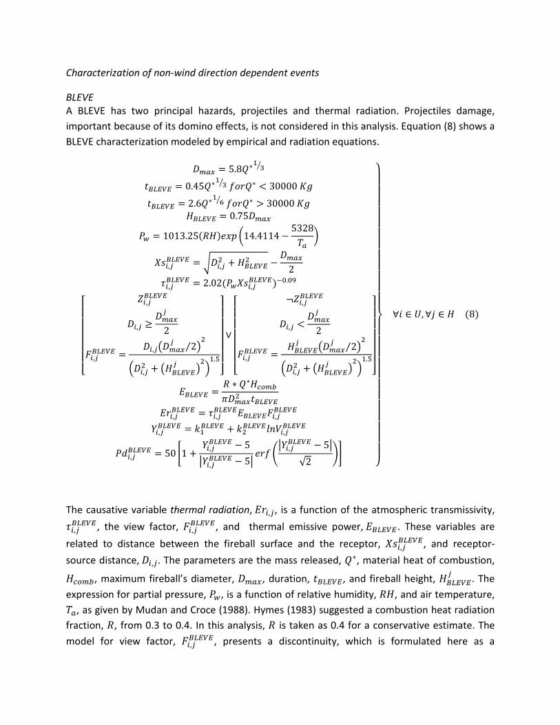
Characterization of non-wind direction dependent events

BLEVE A BLEVE has two principal hazards, projectiles and thermal radiation. Projectiles damage, important because of its domino effects, is not considered in this analysis. Equation (8) shows a BLEVE characterization modeled by empirical and radiation equations.

�

𝐷𝑚𝑎𝑥 = 5.8𝑄∗13�

𝑡𝐵𝐿𝐸𝑉𝐸 = 0.45𝑄∗13� 𝑓𝑜𝑟𝑄∗ < 30000 𝐾𝑔

𝑡𝐵𝐿𝐸𝑉𝐸 = 2.6𝑄∗16� 𝑓𝑜𝑟𝑄∗ > 30000 𝐾𝑔

𝐻𝐵𝐿𝐸𝑉𝐸 = 0.75𝐷𝑚𝑎𝑥

𝑃𝑤 = 1013.25(𝑅𝐻)𝑒𝑥𝑝 �14.4114−5328𝑇𝑎

�

𝑋𝑠𝑖,𝑗𝐵𝐿𝐸𝑉𝐸 = �𝐷𝑖,𝑗2 + 𝐻𝐵𝐿𝐸𝑉𝐸2 −𝐷𝑚𝑎𝑥

2𝜏𝑖,𝑗𝐵𝐿𝐸𝑉𝐸 = 2.02(𝑃𝑤𝑋𝑠𝑖,𝑗𝐵𝐿𝐸𝑉𝐸)−0.09

⎣⎢⎢⎢⎢⎢⎡ 𝑍𝑖,𝑗𝐵𝐿𝐸𝑉𝐸

𝐷𝑖,𝑗 ≥𝐷𝑚𝑎𝑥𝑗

2

𝐹𝑖,𝑗𝐵𝐿𝐸𝑉𝐸 =𝐷𝑖,𝑗�𝐷𝑚𝑎𝑥

𝑗 2⁄ �2

�𝐷𝑖,𝑗2 + �𝐻𝐵𝐿𝐸𝑉𝐸𝑗 �

2�1.5

⎦⎥⎥⎥⎥⎥⎤

∨

⎣⎢⎢⎢⎢⎢⎡ ¬𝑍𝑖,𝑗𝐵𝐿𝐸𝑉𝐸

𝐷𝑖,𝑗 <𝐷𝑚𝑎𝑥𝑗

2

𝐹𝑖,𝑗𝐵𝐿𝐸𝑉𝐸 =𝐻𝐵𝐿𝐸𝑉𝐸𝑗 �𝐷𝑚𝑎𝑥

𝑗 2⁄ �2

�𝐷𝑖,𝑗2 + �𝐻𝐵𝐿𝐸𝑉𝐸𝑗 �

2�1.5

⎦⎥⎥⎥⎥⎥⎤

𝐸𝐵𝐿𝐸𝑉𝐸 =𝑅 ∗ 𝑄∗𝐻𝑐𝑜𝑚𝑏

𝜋𝐷𝑚𝑎𝑥2 𝑡𝐵𝐿𝐸𝑉𝐸𝐸𝑟𝑖,𝑗𝐵𝐿𝐸𝑉𝐸 = 𝜏𝑖,𝑗𝐵𝐿𝐸𝑉𝐸𝐸𝐵𝐿𝐸𝑉𝐸𝐹𝑖,𝑗𝐵𝐿𝐸𝑉𝐸

𝑌𝑖,𝑗𝐵𝐿𝐸𝑉𝐸 = 𝑘1𝐵𝐿𝐸𝑉𝐸 + 𝑘2𝐵𝐿𝐸𝑉𝐸𝑙𝑛𝑉𝑖,𝑗𝐵𝐿𝐸𝑉𝐸

𝑃𝑑𝑖,𝑗𝐵𝐿𝐸𝑉𝐸 = 50 �1 +𝑌𝑖,𝑗𝐵𝐿𝐸𝑉𝐸 − 5�𝑌𝑖,𝑗𝐵𝐿𝐸𝑉𝐸 − 5�

𝑒𝑟𝑓 ��𝑌𝑖,𝑗𝐵𝐿𝐸𝑉𝐸 − 5�

√2��

⎭⎪⎪⎪⎪⎪⎪⎪⎪⎪⎪⎪⎪⎬

⎪⎪⎪⎪⎪⎪⎪⎪⎪⎪⎪⎪⎫

∀𝑖 ∈ 𝑈,∀𝑗 ∈ 𝐻 (8)

The causative variable thermal radiation, 𝐸𝑟𝑖,𝑗, is a function of the atmospheric transmissivity, 𝜏𝑖,𝑗𝐵𝐿𝐸𝑉𝐸 , the view factor, 𝐹𝑖,𝑗𝐵𝐿𝐸𝑉𝐸, and thermal emissive power, 𝐸𝐵𝐿𝐸𝑉𝐸 . These variables are related to distance between the fireball surface and the receptor, 𝑋𝑠𝑖,𝑗𝐵𝐿𝐸𝑉𝐸, and receptor-source distance, 𝐷𝑖,𝑗. The parameters are the mass released, 𝑄∗, material heat of combustion,

𝐻𝑐𝑜𝑚𝑏, maximum fireball’s diameter, 𝐷𝑚𝑎𝑥, duration, 𝑡𝐵𝐿𝐸𝑉𝐸, and fireball height, 𝐻𝐵𝐿𝐸𝑉𝐸𝑗 . The

expression for partial pressure, 𝑃𝑤, is a function of relative humidity, 𝑅𝐻, and air temperature, 𝑇𝑎, as given by Mudan and Croce (1988). Hymes (1983) suggested a combustion heat radiation fraction, 𝑅, from 0.3 to 0.4. In this analysis, 𝑅 is taken as 0.4 for a conservative estimate. The model for view factor, 𝐹𝑖,𝑗𝐵𝐿𝐸𝑉𝐸, presents a discontinuity, which is formulated here as a

disjunction. The BLEVE causative variables, 𝑉𝑖,𝑗𝐵𝐿𝐸𝑉𝐸, and probit constants for workers’ life loss and equipment damage are reported in tables 1, 2 and 3.

Jet fire A jet fire (JF) is produced by the combustion of a pressurized vessel leak. In general, jet fire consequences are considered important only in neighboring areas. As in the BLEVE model, thermal radiation hazard is the main causative variable of this event. Thermal radiation, 𝐸𝑟𝑖,𝑗

𝐽𝐹, is a function of discharge rate, �̇�𝑟, flame size, 𝐿𝑓𝑙𝑎𝑚𝑒, fraction of total energy converted to

radiation, 𝜂𝐽𝐹, heat of combustion, Hcomb, point view factor, 𝐹𝑖,𝑗𝐽𝐹, atmospheric transmissivity,

𝜏𝑖,𝑗𝐽𝐹, and indirectly of distance of receptor-source, 𝐷𝑖,𝑗, and distance from flame center to

receptor, 𝑋𝑠𝑖,𝑗𝐽𝐹. Flame size is a function of molecular weight of air, 𝑀𝑎, molecular weight of fuel,

𝑀𝑓, jet diameter, 𝑑𝑗 , and the fuel mole fraction concentration in a stoichiometric fuel-air

mixture, 𝐶𝑇, see Equation (9). Tables 1, 2 and 3 show the JF probit variables, 𝑉𝑖,𝑗𝐽𝐹, for workers’

life loss and equipment damage.

�

𝐿𝑓𝑙𝑎𝑚𝑒𝑑𝑗

=15𝐶𝑇

�𝑀𝑎

𝑀𝑓

𝑋𝑠𝑖,𝑗𝐽𝐹 = �𝐷𝑖,𝑗2 + 𝐿𝑓𝑙𝑎𝑚𝑒2

𝑃𝑤 = 1013.25(𝑅𝐻)𝑒𝑥𝑝 �14.4114 −5328𝑇𝑎

�

𝜏𝑖,𝑗𝐽𝐹 = 2.02(𝑃𝑤𝑋𝑠𝑖,𝑗

𝐽𝐹)−0.09

𝐹𝑖,𝑗𝐽𝐹 =

14𝜋𝐷𝑖,𝑗2

𝐸𝑟𝑖,𝑗𝐽𝐹 = 𝜏𝑖,𝑗

𝐽𝐹𝜂𝐽𝐹�̇�𝑟 Hcomb𝐹𝑖,𝑗𝐽𝐹

𝑌𝑖,𝑗𝐽𝐹 = 𝑘1

𝐽𝐹 + 𝑘2𝐽𝐹𝑙𝑛𝑉𝑖,𝑗

𝐽𝐹

𝑃𝑑𝑖,𝑗𝐽𝐹 = 50 �1 +

𝑌𝑖,𝑗𝐽𝐹 − 5

�𝑌𝑖,𝑗𝐽𝐹 − 5�

𝑒𝑟𝑓 ��𝑌𝑖,𝑗

𝐽𝐹 − 5�

√2��⎭⎪⎪⎪⎪⎪⎪⎪⎬

⎪⎪⎪⎪⎪⎪⎪⎫

∀𝑖 ∈ 𝑈,∀𝑗 ∈ 𝐻 (9)

Wind direction-dependent scenarios

From bow tie diagrams, scenarios with a delayed ignition are identified. The consequences of such scenarios depend on wind direction and location of ignition sources. In this work, safe

distance, 𝐷𝑠𝑎𝑓𝑒𝑗 , is defined as the distance where the released material cannot be ignited. A

mixture is flammable if it has a concentration between upper and lower flammability limits (UFL-LFL.) Thus, the safety distance is given by the position where concentration in air is lower

than the LFL value. Figure 5 illustrates a material release from dangerous unit j and its unsafe area defined by the largest circle at a concentration equal to LFL. Therefore, ignition can happen in unit i or unit k but not in unit m because unit m is located out of the reach of a flammable mixture.

Wind direction-dependent events require dispersion calculations. Several dispersion models have been proposed (AIChE, 2000; Crowl & Louvar, 2002; Mannan et al., 2005). The dispersion model used in this analysis is the one by Pasquill-Gifford (Gifford, 1982), a simple model that assumes passive dispersion. There are two types of releases with different dispersion phenomena depending on the amount of released material by unit time. We specify the atmospheric conditions, rural conditions and class F stability (very stable), as worst-case conditions.

Equation (10) represents a ground level instantaneous release dispersion model. The average concentration due to instantaneous release, < 𝐶𝑖 >, is a function of the mass released, 𝑄∗, the dispersion coefficients in downwind, crosswind and axial directions (𝜎𝑥, 𝜎𝑦 and 𝜎𝑧), wind velocity, 𝑢, time, 𝑡, and position, (𝑥,𝑦, 𝑧).

�

< 𝐶𝑖 > (𝑥, 0,0, 𝑡) =𝑄∗

√2(𝜋)1.5𝜎𝑥𝜎𝑦𝜎𝑧𝑒𝑥𝑝 �−

12��𝑥 − 𝑢𝑡𝜎𝑥

�2

+𝑦2

𝜎𝑦2+𝑧2

𝜎𝑧2��

𝜎𝑥 = 0.024 ∗ 𝑥0.89

𝜎𝑦 = 0.024 ∗ 𝑥0.89

𝜎𝑧 = 0.05 ∗ 𝑥0.61 ⎭⎪⎬

⎪⎫

(10)

Equation (11) models the dispersion for a point ground level continuous release. The average concentration due to continuous release, < 𝐶𝑐 >, is a function of the leaking flowrate, �̇�𝑟, the dispersion coefficients in downwind, crosswind and axial directions (𝜎𝑥, 𝜎𝑦 and 𝜎𝑧), wind velocity, 𝑢, and position, (𝑥,𝑦, 𝑧). Both instantaneous and continuous dispersion models were taken from Crowl and Louvar (2002).

�

< 𝐶𝑐 > (𝑥,𝑦, 𝑧) =�̇�𝑟

𝜋𝜎𝑦𝜎𝑧𝑢𝑒𝑥𝑝 �−

12�𝑦2

𝜎𝑦2+𝑧2

𝜎𝑧2��

𝜎𝑦 =0.04𝑥

√1 + 0.0001𝑥

𝜎𝑧 =0.016𝑥

1 + 0.0003𝑥 ⎭⎪⎪⎬

⎪⎪⎫

(11)

Values for safe distances are calculated for instantaneous and continuous releases solving equations (10) and (11), respectively, considering a downwind location (𝑥,0,0) and using a

concentration equal to LFL. Then, the safe distance value is obtained, 𝐷𝑠𝑎𝑓𝑒𝑗 = 𝑥, and the unsafe

area is a circle defined by a radius equal to 𝐷𝑠𝑎𝑓𝑒𝑗 and center at the dangerous unit j location.

This model assumes that each unit has ignition sources. Consequently, the probability of ignition depends on wind direction and unit location. The models to characterize consequences from wind-dependent events are described below.

UVCE UVCE is an explosion originated by a release that allows the formation of a cloud that finds an ignition source and gets fired. In Figure 5 for example, a cloud can be ignited in unit I and unit k but not in unit m. Hence, there are no consequences for unit m. However, there are possible consequences for units i and k. If the cloud gets ignited in unit I, the resulting overpressure affects units k and m, Equation (12). A disjunction is proposed to model the consequences, whose occurrence depends on wind direction. The Boolean variable, 𝑍𝑖,𝑗𝑈𝑉𝐶𝐸 , is true if the distance between unit 𝑖 and dangerous unit 𝑗, 𝐷𝑖,𝑗, is less than the safe distance for an

instantaneous release, 𝐷𝑖𝑠𝑎𝑓𝑒𝑗 , and the total damage percentage originated from unit 𝑖, 𝑃𝑑𝑖,𝑗𝑈𝑉𝐶𝐸 ,

is the sum of partial losses in the other units 𝑃𝑝𝑖,𝑘,𝑗𝑈𝑉𝐶𝐸 and in the same unit 𝑃𝑝𝑖,𝑖,𝑗𝑈𝑉𝐶𝐸 . If 𝑍𝑖,𝑗𝑈𝑉𝐶𝐸 is

false, then there are no consequences from UVCE ignited in unit i. The consequences of ignition in unit i is the sum of the damage produced to the others units. For that reason, we formulated a partial probit model that quantifies effects on the other units. Then, a partial probit variable, 𝑌𝑖,𝑘,𝑗

𝑈𝑉𝐶𝐸 , and a partial percentage of damage, 𝑃𝑝𝑖,𝑘,𝑗𝑈𝑉𝐶𝐸 , originated by a release in

unit 𝑗, ignited in unit 𝑖 and received by unit 𝑘 are used. Tables 1, 2 and 3 show the UVCE causative variables, 𝑉𝑖,𝑘,𝑗

𝑈𝑉𝐶𝐸 , and constants for workers’ life loss and equipment damage risk. The main hazard of a UVCE is the overpressure, 𝑝𝑜𝑖,𝑘, originated at location of unit 𝑖 and received

by unit 𝑘. The overpressure 𝑝𝑜𝑖,𝑘 is a function of the mass released, 𝑄∗, fuel heat of

combustion, 𝐻𝑐𝑜𝑚𝑏, and receptor-source distance, 𝐷𝑢𝑖,𝑘. A TNT equivalence model used in this analysis is based on a comparison between the mass and heat of combustion of released material, 𝑄∗𝐻𝑐𝑜𝑚𝑏, and mass and combustion heat of TNT, 𝑊𝐻𝑇𝑁𝑇, considering an efficiency explosion factor, 𝜂𝑈𝑉𝐶𝐸; 𝑎, 𝑏 and 𝑐 are constants related to TNT explosions.

�

𝑊 =𝜂𝑈𝑉𝐶𝐸𝑄∗𝐻𝑐𝑜𝑚𝑏

𝐻𝑇𝑁𝑇𝑍𝑚𝑖,𝑘 =

𝐷𝑢𝑖,𝑘𝑊1 3⁄

𝑙𝑜𝑔10 �𝑝𝑜𝑖,𝑘� = �𝑐𝑖�𝑎 + 𝑏𝑙𝑜𝑔10𝑍𝑚𝑖,𝑘�𝑖

12

𝑖=0𝑎 = −0.2144𝑏 = 1.3503

𝑐𝑖 = [2.7808,−1.6959,−0.1542, 0.5141, 0.0989,−0.2939, 0.0268, 0.1091, 0.0016,−0.0215, 0.0001, 0.0017]

𝑌𝑖,𝑘,𝑗𝑈𝑉𝐶𝐸 = 𝑘1𝑈𝑉𝐶𝐸 + 𝑘2𝑈𝑉𝐶𝐸𝑙𝑛𝑉𝑖,𝑘,𝑗

𝑈𝑉𝐶𝐸

𝑃𝑝𝑖,𝑘,𝑗𝑈𝑉𝐶𝐸 = 50 �1 +

𝑌𝑖,𝑘,𝑗𝑈𝑉𝐶𝐸 − 5

�𝑌𝑖,𝑘,𝑗𝑈𝑉𝐶𝐸 − 5�

𝑒𝑟𝑓 ��𝑌𝑖,𝑘,𝑗

𝑈𝑉𝐶𝐸 − 5�

√2��

𝑃𝑝𝑖,𝑖,𝑗𝑈𝑉𝐶𝐸 = 100

⎣⎢⎢⎢⎢⎡ 𝑍𝑖,𝑗𝑈𝑉𝐶𝐸

𝐷𝑖,𝑗 ≤ 𝐷𝑖𝑠𝑎𝑓𝑒𝑗

𝑃𝑑𝑖,𝑗𝑈𝑉𝐶𝐸 = �𝑃𝑝𝑖,𝑘,𝑗𝑈𝑉𝐶𝐸

𝑈

𝑘 ⎦⎥⎥⎥⎥⎤

∨ �

¬𝑍𝑖,𝑗𝑈𝑉𝐶𝐸

𝐷𝑖,𝑗 > 𝐷𝑖𝑠𝑎𝑓𝑒𝑗

𝑃𝑑𝑖,𝑗𝑈𝑉𝐶𝐸 = 0�

⎭⎪⎪⎪⎪⎪⎪⎪⎪⎪⎪⎬

⎪⎪⎪⎪⎪⎪⎪⎪⎪⎪⎫

∀𝑖,𝑘 ∈ 𝑈,∀𝑗 ∈ 𝐻 (12)

FFC and FFI A flash fire due to a continuous (FFC) or an instantaneous (FFI) release is caused by a flammable mixture of liquid and vapor that ignites. A flash fire is a complex event that does not behave as liquid or as vapor; it lacks a well-accepted characterization model due to the complexity of the occurring physical phenomena. Consequently, the distance of impact is considered as the distance at LFL concentration, and everything inside LFL is considered as a total loss (Rew et al., 1996). Concentration of LFL for instantaneous and continuous releases is calculated with equations (10) and (11), respectively. A disjunction is used to assign percentage of damage to workers and equipment, 𝑃𝑤𝑖,𝑗

𝑒 and 𝑃𝑒𝑖,𝑗𝑒 , Equation (13).

⎣⎢⎢⎢⎡ 𝑍𝑖,𝑗𝑒

𝐷𝑖,𝑗 ≤ 𝐷𝑠𝑎𝑓𝑒𝑃𝑤𝑖,𝑗𝑒 = 100𝑃𝑒𝑖,𝑗𝑒 = 100 ⎦

⎥⎥⎥⎤∨

⎣⎢⎢⎢⎡ ¬𝑍𝑖,𝑗𝑒

𝐷𝑖,𝑗 > 𝐷𝑠𝑎𝑓𝑒𝑃𝑤𝑖,𝑗𝑒 = 0𝑃𝑒𝑖,𝑗𝑒 = 0 ⎦

⎥⎥⎥⎤

∀𝑖 ∈ 𝑈,∀𝑗 ∈ 𝐻, 𝑒 ∈ 𝐹𝐹𝐼,𝐹𝐹𝐶 (13)

Disjunction Reformulation

The models for non-overlapping, wind direction, BLEVE, UVCE, FFC and FFI (Equations (2), (6), (8), (12) and (13)) involve disjunctions. We reformulate the problem using convex hull for

disjunctions that contain linear constraints, and the Big-M method for Equation (8), a non-linear constraint.

The reformulation of non-overlapping disjunctions, Equation (2), is given below in terms of the disaggregated variables 𝑥𝑖,𝑑 and 𝑦𝑖,𝑑,

�

𝑥𝑖 = �𝑥𝑖,𝑑

𝐷

𝑑

𝑦𝑖 = �𝑦𝑖,𝑑

𝐷

𝑑

𝑥𝑖,1 − 𝑥𝑗,1 ≤ −�𝐿𝑖2

+𝐿𝑗2� 𝑧𝑖,𝑗,1

𝑛𝑜

𝑥𝑗,2 − 𝑥𝑖,2 ≤ −�𝐿𝑖2

+𝐿𝑗2� 𝑧𝑖,𝑗,2

𝑛𝑜

𝑦𝑖,3 − 𝑦𝑗,3 ≤ −�𝐻𝑖2

+𝐻𝑗2� 𝑧𝑖,𝑗,3

𝑛𝑜

𝑦𝑗,4 − 𝑦𝑖,4 ≤ −�𝐻𝑖2

+𝐻𝑗2� 𝑧𝑖,𝑗,4

𝑛𝑜

�𝑧𝑖,𝑗,𝑑𝑛𝑜

𝐷

𝑑

= 1

0 ≤ 𝑥𝑖,𝑑 ≤ 𝑈𝑥𝑖 ∗ 𝑧𝑖,𝑗,𝑑𝑛𝑜

0 ≤ 𝑦𝑖,𝑑 ≤ 𝑈𝑦𝑖 ∗ 𝑧𝑖,𝑗,𝑑𝑛𝑜 ⎭

⎪⎪⎪⎪⎪⎪⎪⎪⎪⎬

⎪⎪⎪⎪⎪⎪⎪⎪⎪⎫

∀𝑖, 𝑗 ∈ 𝑈 ∪ 𝐻, 𝑖 < 𝑗 (14)

The wind rose disjunction within Equation (6) is transformed into:

�

𝑎𝑛𝑔𝑙𝑒𝑖,𝑗 = �𝑎𝑛𝑔𝑙𝑒𝑖,𝑗,𝑠

𝑆

𝑠

𝑃𝑒𝑗 = �𝑃𝑒,𝑠

𝑗𝑆

𝑠𝑎𝑛𝑔𝑙𝑒𝑖,𝑗,𝑠 ≥ 𝐿𝐴𝑠𝑧𝑠𝑤𝑟

𝑎𝑛𝑔𝑙𝑒𝑖,𝑗,𝑠 ≤ 𝑈𝐴𝑠𝑧𝑠𝑤𝑟

𝑃𝑒,𝑠𝑗 = 𝑃𝑒𝑏𝑜𝑤𝑡𝑖𝑒𝑃𝑓𝑠 𝑧𝑠𝑤𝑟

�𝑧𝑠𝑤𝑟𝑆

𝑠

= 1

𝐿𝑎𝑛𝑔𝑙𝑒𝑖,𝑗 𝑧𝑠𝑤𝑟 ≤ 𝑎𝑛𝑔𝑙𝑒𝑖,𝑗,𝑠 ≤ 𝑈𝑎𝑛𝑔𝑙𝑒𝑖,𝑗 ∗ 𝑧𝑠𝑤𝑟

0 ≤ 𝑃𝑒,𝑠𝑗 ≤ 𝑈𝑃𝑒

𝑗 𝑧𝑠𝑤𝑟 ⎭⎪⎪⎪⎪⎪⎪⎬

⎪⎪⎪⎪⎪⎪⎫

∀𝑖 ∈ 𝑈,∀𝑗 ∈ 𝐻,∀𝑒 ∈ 𝑊𝑅 (15)

The disjunction within the UVCE model becomes,

�

𝐷𝑖,𝑗 = �𝐷𝑖,𝑗,𝑙

2

𝑙=1

𝑃𝑝𝑖,𝑘,𝑗𝑈𝑉𝐶𝐸 = �𝑃𝑝𝑖,𝑘,𝑗,𝑙

𝑈𝑉𝐶𝐸2

𝑙=1

𝑃𝑑𝑖,𝑘,𝑗𝑈𝑉𝐶𝐸 = �𝑃𝑑𝑖,𝑗,𝑙

𝑈𝑉𝐶𝐸2

𝑙=1

𝐷𝑖,𝑗,1 ≤ 𝐷𝑖𝑠𝑎𝑓𝑒𝑗 ∗ 𝑧𝑖,𝑗,1

𝑈𝑉𝐶𝐸

𝑃𝑑𝑖,𝑗,1𝑈𝑉𝐶𝐸 = �𝑃𝑝𝑖,𝑘,𝑗,1

𝑈𝑉𝐶𝐸 ∗ 𝑧𝑖,𝑗,1𝑈𝑉𝐶𝐸

𝑈

𝑘𝐷𝑖,𝑗,2 > 𝐷𝑠𝑎𝑓𝑒 ∗ 𝑧𝑖,𝑗,2

𝑈𝑉𝐶𝐸

𝑃𝑑𝑖,𝑗,2𝑈𝑉𝐶𝐸 = 0

0 ≤ 𝐷𝑖,𝑗,𝑙 ≤ 𝑈𝐷𝑖,𝑗𝑧𝑖,𝑗,𝑙𝑈𝑉𝐶𝐸

0 ≤ 𝑃𝑝𝑖,𝑘,𝑗,𝑙𝑈𝑉𝐶𝐸 ≤ 𝑈𝑃𝑝𝑖,𝑘,𝑗

𝑈𝑉𝐶𝐸𝑧𝑖,𝑗,𝑙𝑈𝑉𝐶𝐸

0 ≤ 𝑃𝑑𝑖,𝑗,𝑙𝑈𝑉𝐶𝐸 ≤ 𝑈𝑃𝑑𝑖,𝑗𝑈𝑉𝐶𝐸𝑚𝑎𝑥𝑧𝑖,𝑗,𝑙

𝑈𝑉𝐶𝐸⎭⎪⎪⎪⎪⎪⎪⎪⎪⎪⎬

⎪⎪⎪⎪⎪⎪⎪⎪⎪⎫

∀𝑖,𝑘 ∈ 𝑈, 𝑖 < 𝑘,∀𝑗 ∈ 𝐻 (16)

The disjunction for consequences for FFC and FFI effects is reformulated as,

�

𝐷𝑖,𝑗 = �𝐷𝑖,𝑗,𝑘

2

𝑘=1

𝑃𝑤𝑖,𝑗𝑒 = �𝑃𝑤𝑖,𝑗,𝑘𝑒

2

𝑘=1

𝑃𝑒𝑖,𝑗𝑒 = �𝑃𝑒𝑖,𝑗,𝑘𝑒

2

𝑘=1𝐷𝑖,𝑗,1 ≤ 𝐷𝑠𝑎𝑓𝑒 ∗ 𝑧𝑖,𝑗,1

𝑒

𝑃𝑤𝑖,𝑗,1𝑒 = 100 ∗ 𝑧𝑖,𝑗,1

𝑒

𝑃𝑒𝑖,𝑗,1𝑒 = 100 ∗ 𝑧𝑖,𝑗,1

𝑒

𝐷𝑖,𝑗,2 > 𝐷𝑠𝑎𝑓𝑒 ∗ 𝑧𝑖,𝑗,1𝑒

𝑃𝑤𝑖,𝑗,2𝑒 = 0

𝑃𝑒𝑖,𝑗,2𝑒 = 0

�𝑧𝑖,𝑗,𝑘𝑒

2

𝑘=1

= 1

0 ≤ 𝐷𝑖,𝑗,𝑘 ≤ 𝑈𝐷𝑖,𝑗𝑧𝑖,𝑗,𝑘𝑒

0 ≤ 𝑃𝑤𝑖,𝑗,𝑘𝑒 ≤ 𝑈𝑃𝑤𝑖,𝑗𝑒 𝑧𝑖,𝑗,𝑘

𝑒

0 ≤ 𝑃𝑒𝑖,𝑗,𝑘𝑒 ≤ 𝑈𝑃𝑒𝑖,𝑗𝑒 𝑧𝑖,𝑗,𝑘

𝑒 ⎭⎪⎪⎪⎪⎪⎪⎪⎪⎪⎪⎬

⎪⎪⎪⎪⎪⎪⎪⎪⎪⎪⎫

∀𝑖 ∈ 𝑈,∀𝑗 ∈ 𝐻, 𝑒 ∈ 𝐹𝐹𝐼,𝐹𝐹𝐶 (17)

For the BLEVE scenario, a Big-M model is used,

�

𝐷𝑖,𝑗 ≥𝐷𝑚𝑎𝑥𝑗

2−𝑀�1 − 𝑧𝑖,𝑗,1

𝐵𝐿𝐸𝑉𝐸�

𝐹𝑖,𝑗𝐵𝐿𝐸𝑉𝐸 >𝐷𝑖,𝑗�𝐷𝑚𝑎𝑥

𝑗 2⁄ �2

�𝐷𝑖,𝑗2 + �𝐻𝐵𝐿𝐸𝑉𝐸𝑗 �

2�1.5 − 𝑀�1 − 𝑧𝑖,𝑗,1

𝐵𝐿𝐸𝑉𝐸�

𝐹𝑖,𝑗𝐵𝐿𝐸𝑉𝐸 <𝐷𝑖,𝑗�𝐷𝑚𝑎𝑥

𝑗 2⁄ �2

�𝐷𝑖,𝑗2 + �𝐻𝐵𝐿𝐸𝑉𝐸𝑗 �

2�1.5 + 𝑀�1 − 𝑧𝑖,𝑗,1

𝐵𝐿𝐸𝑉𝐸�

𝐷𝑖,𝑗 <𝐷𝑚𝑎𝑥𝑗

2+ 𝑀�1 − 𝑧𝑖,𝑗,2

𝐵𝐿𝐸𝑉𝐸�

𝐹𝑖,𝑗𝐵𝐿𝐸𝑉𝐸 >𝐻𝐵𝐿𝐸𝑉𝐸𝑗 �𝐷𝑚𝑎𝑥

𝑗 2⁄ �2

�𝐷𝑖,𝑗2 + �𝐻𝐵𝐿𝐸𝑉𝐸𝑗 �

2�1.5 − 𝑀�1 − 𝑧𝑖,𝑗,2

𝐵𝐿𝐸𝑉𝐸�

𝐹𝑖,𝑗𝐵𝐿𝐸𝑉𝐸 <𝐻𝐵𝐿𝐸𝑉𝐸𝑗 �𝐷𝑚𝑎𝑥

𝑗 2⁄ �2

�𝐷𝑖,𝑗2 + �𝐻𝐵𝐿𝐸𝑉𝐸𝑗 �

2�1.5 + 𝑀�1 − 𝑧𝑖,𝑗,2

𝐵𝐿𝐸𝑉𝐸�

⎭⎪⎪⎪⎪⎪⎪⎪⎪⎬

⎪⎪⎪⎪⎪⎪⎪⎪⎫

∀𝑖 ∈ 𝑈,∀𝑗 ∈ 𝐻 (18)

Objective function

The objective function is the minimization of the Plant Layout Cost, 𝑃𝐿𝐶, which includes the effects of societal risk and equipment risk, plus the units distance of interconnection times interconnection costs, and land cost times occupied area:

𝑃𝐿𝐶 = ���𝑅𝑠𝑜𝑐𝑖𝑒𝑡𝑎𝑙𝑖,𝑗 ∗ 𝐶𝑝𝑟𝑒𝑣

𝑈

𝑖

∗ 𝐿𝑝𝑟𝑜𝑗 + �𝑅𝑒𝑞𝑢𝑖𝑝𝑚𝑒𝑛𝑡𝑖,𝑗 ∗ 𝐶𝑒𝑞𝑢𝑖𝑝𝑚𝑒𝑛𝑡

𝑖𝑈

𝑖

∗ 𝐿𝑝𝑟𝑜𝑗 + �𝐷𝑖,𝑗

𝑈

𝑖

∗ 𝐶𝑐𝑜𝑛𝑖,𝑗 �

𝐻

𝑗

+ 𝐶𝑙𝑎𝑛𝑑𝐴𝑙𝑎𝑛𝑑 (19)

The mixed-integer non linear optimization model consists in the minimization of the objective function Equation (19) subject to the geometry relations Equation (1), the reformulation of non-overlapping disjunction Equation (14), the risk definitions Equation (3), the frequency analysis Equations (4) and (5), the wind rose Equation (6) and its reformulation Equation (15), the BLEVE consequences model Equation (8) and the reformulation Equation (18), JF consequences model Equation (9), UVCE consequences model Equation (12) and its convex hull disjunction reformulation Equation (16), and finally FFI and FFC consequences models Equation (13) and reformulation Equation (17). The model was solved using DICOPT with the GAMS software environment (Brooke et al., 2006)

Case studies

Two case studies are presented. The first case study was adapted from the CPQRA example reported in the CCPS Guidelines (AIChE, 2000). A hydrocarbon separation unit of n-hexane/n-heptane is considered as the dangerous unit due to a large amount of flammable material. A flat area of 250 m in the east direction and 500 m in the north direction is considered. Land cost is equal to $6/m2. The separation unit is located in the middle, at point (125,250). In addition to the separation unit, a small storage atmospheric tank, an office building and the main control room need to be located. General parameters for the units are given in Table 4, including dimensions, people near unit, equipment and interconnection costs.

CCPS guidelines report that the mass of n-hexane released is equal to 28,000 Kg for an instantaneous release, and a flow of 11 Kg/s for a continuous release. For dispersion calculations, a wind velocity of 1.5 m/s is taken as a worst-case scenario to provide conservative results. Figure 6 shows the wind rose provided for the site in the CCPS book; the 360 degrees were divided into eight slices, with boundaries shown in Table 5. In addition, there are restrictions for safety distances between units considered in the model. Table 6 shows reported values for common industry safety distances (AIChE, 2003).

Bowtie graphs were developed based on the fault and event trees reported in the CCPS book, and the results are shown in Figures 3 and 4; there are five possible events for this case, BLEVE, UVCE, FFI, JF and FFC. For the bow tie analysis, failure rates and expert judgment probabilities were taken from the Rijnmond area report (COVO Committee, 1982) and the CCPS book, with a length of 25m for large pipeline and 55m for medium pipeline. As part of the model solution, the outcomes can be categorized by their probabilities of occurrence as given in Table 7. Jet fire is the most probable event and a vapor cloud explosion and flash fire due to an instantaneous release are the least probable.

In addition, the CCPS book reports that UVCE and BLEVE present the largest death rate. In general, the worst-case scenario is considered as either the most probable or the highest consequences scenario. Some approaches consider the highest consequences scenario for conservative results. However, without a QRA it is difficult to define which scenario is the most probable and which one has the worst consequences. In this work the layout optimization was performed considering all catastrophic outcomes as identified from a bowtie analysis. The MINLP model for this problem involves 123 0-1 variables, 536 continuous variables and 1234 constraints, and the solution took 7.83 sec of CPU time with DICOPT.

The resulting layout is presented in Figure 7. The fixed location for the distillation unit DU (dangerous unit) is (125,250). All units meet safety distances criteria. Center locations for units 1, 2 and 3 are (145,325.69), (130,485), and (120,439.92). The objective function value was

$116,406, considering a project life of 5 years. The final occupied area 𝐴𝑙𝑎𝑛𝑑, yellow rectangle, is equal to 10,600 m2, distributed in 40 m in the east direction and 265 m in the north direction. As expected, Unit 1, small storage, is the closest unit to the dangerous equipment due to the interconnection penalty. Unit 2, Office, is the most distant from the dangerous equipment due to the number of people therein. The final layout locates all units in a low wind direction probability.

The model was also solved considering outcomes individually. In Figure 8, individual objective function values for each outcome are shown, together with the total objective function (𝑃𝐿𝐶). A jet fire is the most common incident, but it has the smallest footprint. Therefore, the layout obtained considering only jet fire has the largest 𝑃𝐿𝐶, because it shows the lowest consequences from all of the other events, and as a result the risk is underestimated. On the other hand, UVCE shows the largest contour impact, and its layout does not yield the most conservative results. Indeed, only the BLEVE scenario provides a conservative result in terms of safety.

Figure 9 (a) shows the cost contribution to the objective function. The BLEVE layout has the lowest societal risk cost, which means that it provides the safest layout solution. However, the solution considering all outcomes has the lowest PLC value. An important aspect to consider is the contributing factors to the objective function. The weight on the objective function of equipment risk cost and interconnection is not as important as land cost and societal risk cost for all cases. The occupied area and societal risk are variables in conflict within the objective function. Such conflict was analyzed varying the land cost parameter within the optimization and monitoring both societal risk and occupied area. The resulting Pareto front is given in Figure 9(b). The societal risk varies from 9/1000 to 20/1000 dead workers. The weight factors, land cost and cost of prevention of life loss, have an important impact in the layout results.

The results from this test demonstrate that considering individual worst-case scenario provides a more expensive layout than a simultaneous consideration.

Case Study 2

This case study is an extension of case study 1 and it was taken from Jung et al. (2010a) These authors used a grid-based model to generate their solution. There are six units to be located, a main control room, an office, an auxiliary building for maintenance, two small atmospheric tanks and a utilities facility, along with two dangerous units, a distillation unit (DU) and a large storage tank (LST). Table 8 describes the general parameters for this case. The properties of distillation unit (DU) are the same as in Example 1 but with different dimensions, 20x20 m. The other dangerous unit, LST, contains 33,000 Kg of n-hexane to be considered for an instantaneous release, and can provide a flow rate of 6 Kg/s in the case of a continuous release.

An available flat area of 250x250 m2 is considered. DU is located at coordinates (125,125) and LST at (110,130). All units are connected with the distillation unit but not with the storage tank (hence cost of LST interconnection is zero). The land cost is $6/m2.

Table 9 shows reported values for common industry safety distances (AIChE, 2003). These restrictions are included within the model as lower limits for distances between units.

The bow tie graphs for DU and LST are considered the same as in Example 1, see Figures 3 and 4. Thus, the total number of scenarios is ten, BLEVE, UVCE, FFI, JF and FFC for each dangerous unit. As mentioned above, identifying the worst-case scenario becomes a non-trivial task when the number of dangerous units increases. Failures rates for LST are considered equal to those for DU, see Table 7. Figure 6 shows the wind rose provided for the site in the CCPS book; the 360 degrees were divided into five slices, with boundaries shown in Table 10. The corresponding MINLP model involved 264 binary variables, 1704 continuous variables and 3766 constraints, and was solved in 63.2 sec using DICOPT.

Figure 10 shows the optimal layout predicted by the proposed model, with a cost of $125651. This result includes the Euclidean safety distances constraints that the solution from the model by Jung et al. (2010a) cannot handle. It should be pointed out that we used their solution as an initial point, but it was infeasible for our model because the distance between Unit 2, Office, and the LST is lower than the safety Euclidean distance specified here. The problem is that Jung et al. used Manhattan distances in order to generate a linear model, and seemingly did not recalculate the corresponding Euclidean distances to check for feasibility. In our case, Euclidean distances are used, which contributes to the nonlinearities of the model in exchange for a better precision. As expected, the U2 Office is the farthest unit from the dangerous units LST and DU. The six optimal units coordinates are: main control room (207.4, 156.1), office (245, 79.9), maintenance building (217.4, 156.1), small tank 1 (121.1, 156.1), small tank 2 (155.9, 130) and utilities facility (152.5, 140). The total occupied area is equal to 13628.85m2 (145mx86.19m).

Conclusions

A new MINLP model for an optimal layout considering a quantitative risk analysis has been proposed. The model can be formulated with fixed facilities (already installed) and/or new facilities. A systematic approach has been used for the integration of economics considerations and uncertain risk scenarios within the optimization procedure. A risk analysis considering flammable material releases is included. A wind rose analysis for the site was considered within the model. Instead of using a predetermined worst-case scenario, a bowtie analysis is developed for each dangerous unit. It was shown that such an approach provides an improvement over models based on worst-case scenarios. Also, the model allows allocating

units at any available space and evaluates that location convenience within the objective function, which provides a noticeable advantage over grid-based models.

Acknowledgements

N. Medina-Herrera was supported for a seven-month stay at Carnegie Mellon University as part of the mixed-scholarship program from the National Science for Science and Technology (CONACYT), Mexico.

References

AIChE (2003). Guidelines for Facility Siting and Layout. Center for Chemical Process Safety/AIChE, New York, NY. AIChE (2000). Guidelines for Chemical Process Quantitative Risk Analysis. 2 ed., AIChE, New York, New York, p 756. Brooke, A., Kendrick, D., Meeruas, A., & Raman, R. (2006). GAMS-language guide. Washington, DC: GAMS Development Corporation COVO Committee (1982). Risk Analysis of Six Potentially Hazardous Objects in the Rijnmond Area, a Pilot Study. D. Reidel Publishing Company, Dorderecht, Holland. Crowl, D.A., & Louvar, J. F. (2002). Chemical Process Safety Fundamentals with Applications. Second ed.; Prentice Hall International Series. Georgiadis, M. C., Schilling, G., Rotstein, G. E., & Macchietto, S. (1999). A general mathematical programming approach for process plant layout. Computers & Chemical Engineering, 23 (7), 823-840. Gifford, F. A. (1982). Horizontal diffusion in the atmosphere: A Lagrangian-dynamical theory. Atmospheric Environment (1967), 16 (3), 505-512. Hymes, I. (1983). The physiological and pathological effects of thermal radiation, SRD R275 . Office, H. S., Ed. London. Jung, S., Ng, D., Laird, C. D., & Mannan, M. S. (2010). A new approach for facility siting using mapping risks on a plant grid area and optimization. Journal of Loss Prevention in the Process Industries, 23 (6), 824-830. Jung, S., Ng, D., Lee, J.-H., Vazquez-Roman, R., & Mannan, M. S. (2010). An approach for risk reduction (methodology) based on optimizing the facility layout and siting in toxic gas release scenarios. Journal of Loss Prevention in the Process Industries, 23 (1), 139-148. Landucci, G., Gubinelli, G., Antonioni, G., & Cozzani, V. (2009). The assessment of the damage probability of storage tanks in domino events triggered by fire. Accident Analysis & Prevention, 41 (6), 1206-1215. Mannan, S., Lees, F. P., & Knovel (Firm). (2005). Lees' loss prevention in the process industries hazard identification, assessment, and control. 3rd ed., Elsevier Butterworth-Heinemann: Amsterdam, Boston. http://www.knovel.com/knovel2/Toc.jsp?BookID=1470.

Marx, J. D., & Cornwell, J. B. (2009). The importance of weather variations in a quantitative risk analysis. Journal of Loss Prevention in the Process Industries, 22 (6), 803-808. Meel, A., & Seider, W. D. (2008). Real-time risk analysis of safety systems. Computers & Chemical Engineering, 32 (4–5), 827-840. Meel, A., Seider, W. D., & Oktem, U. (2008). Analysis of management actions, human behavior, and process reliability in chemical plants. II. Near-miss management system selection. Process Safety Progress, 27 (2), 139-144. Mingguang, Z., & Juncheng, J. (2008). An improved probit method for assessment of domino effect to chemical process equipment caused by overpressure. Journal of Hazardous Materials, 158 (2–3), 280-286. Modarres, M., Kaminskiy, M., & Krivtsov, V. (2010). Reliability engineering and risk analysis : A practical guide. 2nd ed., CRC Press: Boca Raton. Mudan, K. S., & Croce, P.A. (1988). Fire Hazard Calculations for Large Open Hydrocarbon Fires. Nation Fire Protection Association, Quincy, MA. Ni, H., Chen, A., & Chen, N. (2010). Some extensions on risk matrix approach. Safety Science, 48 (10), 1269-1278. Patsiatzis, D. I., Knight, G., & Papageorgiou, L. G. (2004). An MILP Approach to Safe Process Plant Layout. Chemical Engineering Research and Design, 82 (5), 579-586. Penteado, F. D., & Ciric, A. R. (1996). An MINLP Approach for Safe Process Plant Layout. Industrial & Engineering Chemistry Research, 35 (4), 1354-1361. Rew, P.J., Deaves, D.M., Hockey, S.M., & and Lines, I.G.. (1996). Review of Flash Fire Modelling. HSE Contract Research Report No. 94/1996. Sawaya, N., & Grossmann, I.E. (2012). A hierarchy of relaxations for linear generalized disjunctive programming. European Journal of Operational Research, 216 (1), 70-82. Vázquez-Román, R., Lee, J.-H., Jung, S., & Mannan, M. S. (2010). Optimal facility layout under toxic release in process facilities: A stochastic approach. Computers & Chemical Engineering, 34 (1), 122-133. Venkatasubramanian, V., Rengaswamy, R., Yin, K., & Kavuri, S. N. (2003a). A review of process fault detection and diagnosis: Part I: Quantitative model-based methods. Computers & Chemical Engineering, 27 (3), 293-311. Venkatasubramanian, V., Rengaswamy, R., & Kavuri, S. N. (2003b). A review of process fault detection and diagnosis: Part II: Qualitative models and search strategies. Computers & Chemical Engineering, 27 (3), 313-326. Venkatasubramanian, V., Rengaswamy, R., Kavuri, S. N., & Yin, K. (2003c). A review of process fault detection and diagnosis: Part III: Process history based methods. Computers & Chemical Engineering, 27 (3), 327-346.

Table 1 Probit model parameters for loss of workers’ life (𝑷𝒘𝒊,𝒋𝒆 )

Event (e) 𝒌𝟏𝒆 𝒌𝟐𝒆 𝑽𝒊,𝒋𝒆 Thermal Radiation*

(BLEVE, JET FIRE) −14.9 2.56

�𝑡𝑒 ∗ �𝐸𝑟𝑖,𝑗𝑒 �

4/3

104�

Overpressure* (UVCE)

−77.1 6.91 𝑝𝑜𝑖,𝑘

*Source: AIChE (2000)

Table 2 Probit model parameters for damage to atmospheric equipment (𝑷𝒆𝒊,𝒋𝒆 )

Event (e) 𝒌𝟏 𝒌𝟐 𝑽 Thermal Radiation*

(BLEVE, JET FIRE) 9.25 − 1.85 (𝑡𝑡𝑓/60)

Where : 𝑙𝑛(𝑡𝑡𝑓) = −1.13𝑙𝑛�𝐸𝑟𝑖,𝑗𝑒 � − 2.67𝑥10−5𝑉𝑜𝑙

+ 9.9 Overpressure**

(UVCE) −9.36 1.43 𝑝𝑜𝑖,𝑘

*Source: Landucci et al. (2009)

**Source: Mingguang & Juncheng (2008)

Table 3 Probit model parameters for damage to pressurized equipment (𝑷𝒆𝒊,𝒋𝒆 )

Event (e) 𝒌𝟏 𝒌𝟐 𝑽 Thermal Radiation*

(BLEVE, JET FIRE) 9.25 − 1.85 (𝑡𝑡𝑓/60)

Where : 𝑙𝑛(𝑡𝑡𝑓) = −0.95𝑙𝑛�𝐸𝑟𝑖,𝑗𝑒 � + 8.845𝑉𝑜𝑙0.032

Overpressure** (UVCE)

−14.44 1.82 𝑝𝑜𝑖,𝑘

*Source: Landucci et al. (2009)

**Source: Mingguang & Juncheng (2008)

Table 4 General parameters for units

Unit Dimension x x y (m)

People Nearby

Cost of unit or equipment ($)

Cost of interconnection

($/m) Distillation unit

(dangerous unit) 30x30 0 -- --

1. Small storage atmospheric tank 10x10 1 100000 100

2. Office 40x30 200 300000 0.1 3. Main control room 20x10 10 1000000 10

Table 1 Slice boundaries

Slice LAs (degrees)

UAs (degrees) 𝑷𝒇𝒔

1 0 45 0.1 2 45 90 0.1 3 90 135 0.1 4 135 180 0.1 5 180 225 0.15 6 225 270 0.2 7 270 315 0.15 8 315 360 0.1

Table 2 Safety distances

Units Small Storage Main control room 30 m

Office 15 m

Table 7 Outcomes bowtie probability of occurrence

Outcome JF FFC BLEVE UVCE FFI 𝐏𝐞𝐃𝐔 3.67x10-5 2.47x10-5 5.75x10-6 7.76x10-7 7.76x10-7

Table 8 General parameters for case study 2

Unit Dimension People Nearby

Equipment Cost ($)

Interconnection ($/m)

U1. Main control 10x10 10 1000000 10 U2. Office 10x10 200 300000 0.1

U3. Auxiliary building for maintenance

10x10 10 200000 2

U4. Small volume storage tank 1 10x10 1 100000 100 U5. small volume storage tank 2 10x10 1 100000 100

U6. Utility 10x10 5 500000 50 DU. Distillation unit 20x20 - - -

LST. Large volume storage tank 10x10 - - -

Table 9 Safety distances

Units Small Storage (U4,U5)

Utility building (U6)

Distillation Unit (DU)

Large Tank (LST)

Main control room(U1) 30 m 30 m 50 m 76 m Office(U2) 15 m 30 m 50 m 76 m

Maintenance building(U3) 15 m 30 m 50 m 76 m

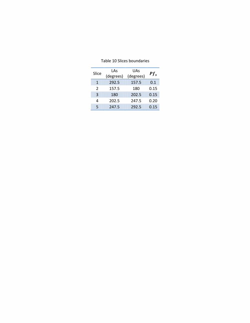
Table 10 Slices boundaries

Slice LAs (degrees)

UAs (degrees) 𝑷𝒇𝒔

1 292.5 157.5 0.1 2 157.5 180 0.15 3 180 202.5 0.15 4 202.5 247.5 0.20 5 247.5 292.5 0.15

CAPTIONS FOR FIGURES

Figure 1. Graphic representation of a Quantitative Risk Analysis

Figure 2. Non-overlapping possibilities for the placement of unit i with respect to unit j; right, left, above and below

Figure 3. Instantaneous Release Bow tie

Figure 4. Continuous Release Bow tie

Figure 5. Graphical representation of safe distances

Figure 6. Wind rose diagram for case study 1

Figure 7. Optimal layout for case study 1 considering all outcomes

Figure 8. Model solution considering individual outcomes

Figure 9. Additional results for case study 1. (a) Contributions to the objective function considering individual and all outcomes. (b) Area-societal risk tradeoff

Figure 10. Optimal layout obtained for case study 2

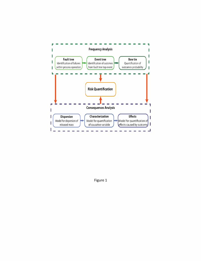
Figure 1

Figure 2

Figure 3

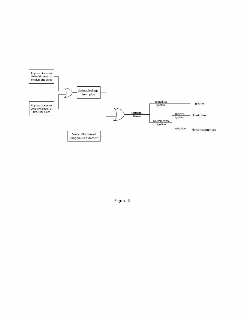
Figure 4

Figure 5

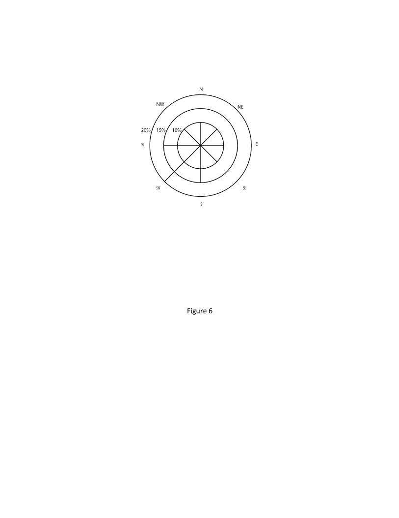
Figure 6

Figure 7

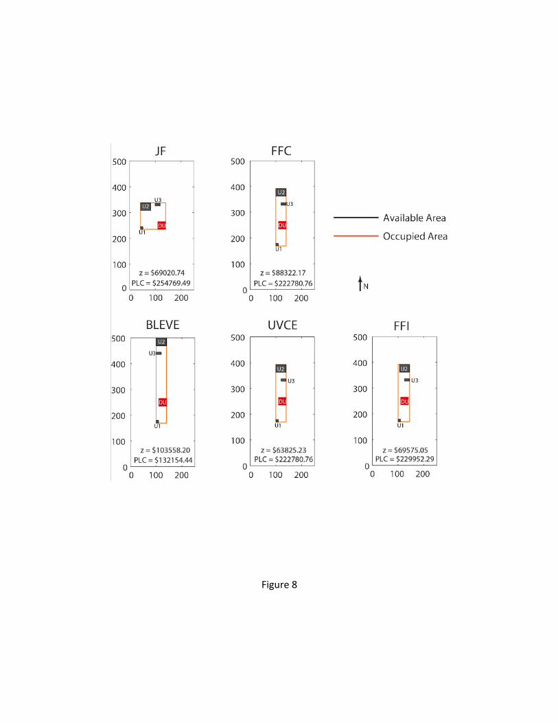
Figure 8

Figure 9

Figure 10