optimal layout of multi-floor process plants using milp

OPTIMAL LAYOUT OF MULTI-FLOOR PROCESS

PLANTS USING MILP

Jude O. Ejeha, Songsong Liub, Lazaros G. Papageorgioua,∗

aCentre for Process Systems Engineering, Department of Chemical Engineering, University

College London, Torrington place, London WC1E 7JE, UKbSchool of Management, Swansea University, Bay Campus, Fabian Way, Swansea SA1

8EN, UK

Abstract

In this work, a new mixed integer linear programming (MILP) model is proposedfor the multi-�oor process plant layout problem with additional considerations.Multi-�oor process plant layout determines the spatial arrangement of processplant units considering their connectivity amongst other factors and a�ects thecost of constructing the plant, the ease of plant operation and expansion, gen-eral safety levels within the plant and its neighbouring environment, as wellas operational costs. Over the past years, mathematical programming modelshave been developed to describe the layout problem considering connectivitycosts, pumping costs, installation of safety devices, and piping, in single andmultiple �oors. Features such the representation of irregularly shaped items,tall equipment spanning multiple �oors and others have been successfully mod-elled. This work builds on such past considerations with additional featuresthat allow multi-�oor equipment items extend above the maximum potentialnumber of �oors, and the selection of an available number of �oors less than themaximum number required by any equipment item. Integer cuts are also de-veloped for the proposed model to enhance its e�ciency. The performance andlimitations of the proposed model are demonstrated with industry-relevant casestudies of up to 25 units, and results show a potential cost savings when com-pared to existing models with additional computational bene�ts of the integercuts in all of the cases explored.

Keywords: multi-�oor process plant layout, mixed integer linear programming(MILP), optimisation

1. Introduction

There has been an upward trend in the cost of land as well as a growingconcern of space availability not just for the establishment of new chemical pro-

∗Corresponding author. Tel: +44 (0)20 7679 2563Email address: [email protected] (Lazaros G. Papageorgiou)

Preprint submitted to Elsevier Thursday 19th September, 2019

cess plants but for the expansion of existing ones (Hosseini-Nasab et al., 2018).This, combined with the ever increasing need to operate chemical process plantsat reduced costs and increased e�ciency without compromising general safetylevels, has given more focus to the layout design of chemical process plants.Layout design determines how all equipment and/or structures in a chemicalprocess plant are spatial arranged with their associated interconnections. Agood layout design provides a healthy balance of e�cient, safe and economicplant construction, operation, use of space and compliance with relevant laws,codes and standards, amongst other factors (Moran, 2017).Each of these factors has, one way or the other, been incorporated over the yearsin mixed integer (non)linear programming (MI(N)LP) models in a bid to obtainoptimal layout designs for any given process plant. Penteado and Ciric (1996)focused on an optimal layout design that balanced safety and economics. Theproposed MINLP model minimised overall costs for piping, land, �nancial riskand the installation of protection devices for a single �oor layout. Financial riskwas estimated based on the expected �nancial losses associated with the sever-ity and probability of an accident. Georgiadis and Macchietto (1997) proposedan MILP formulation discretising the �oor area with considerations for con-nection, �oor construction and pumping costs. The model handled multi-�oor�oor layout and a heuristic was also proposed for large-sized problems. Theheuristic selected units based on their degree of connectivity, starting with the�rst two units being �xed at a central location and iteratively solving for an ad-ditional unit until all were allocated. The limitations of the space discretisationapproach by Georgiadis and Macchietto (1997) was addressed by Papageorgiouand Rotstein (1998) in a continuous space MILP model but for a single �oorlayout. The authors also considered the pre-allocation of equipment items toproduction sections. Further work was done by Barbosa-Póvoa et al. (2002)for multi-�oor scenarios having irregularly shaped equipment items, multipleinput and output connection points, variable number of �oors with variable�oor heights in 3-dimensional space. Irregular equipment items were modelledas a combination of a prede�ned number of rectangular objects. Patsiatzis andPapageorgiou (2002) further included area-dependent land purchase and �oorconstruction costs for 3-dimensional layouts in an MILP model. Guirardelloand Swaney (2005) included the feature of pipe routing and pipe layout, andPatsiatzis et al. (2005) investigated the layout aspects of pipeless batch plant.Additional safety considerations have also been included in the layout modelover and above the minimum separation distances earlier adopted. Principlesfrom the Dow's �re and explosion index guide (American Institute of ChemicalEngineers, 1994) were incorporated into an MILP model by Patsiatzis et al.(2004) in estimating risk levels within a plant, and more recently, the DominoHazard index has also been adopted to model potential hazardous events thatcan be mitigated with proper layout considerations (Brunoro Ahumada et al.,2018, de Lira-Flores et al., 2014, López-Molina et al., 2013, Tugnoli et al., 2008).In the later case, the domino e�ect of hazardous scenarios such as �ash �re, �re-ball, pool and jet �res, and explosions were formulated as an MINLP (López-Molina et al., 2013, de Lira-Flores et al., 2014) or MILP (Brunoro Ahumada

2

et al., 2018) model, with an overall objective to minimize the total layout costs,damage costs and purchase of protection devices.In recent times, owing to problems of scalability, heuristics, the use of evolu-tionary techniques and the combination of both have been developed for thelayout problem. Previous simultaneous approaches were only able to solvelayout problems having less than 11 units in reasonable computational times.Decomposition approaches (Patsiatzis and Papageorgiou, 2003), construction-based methods (Xu and Papageorgiou, 2007) with improvement phases (Xuand Papageorgiou, 2009), and a number of evolutionary methods (Furuholmenet al., 2010, Kheirkhah et al., 2015, Nabavi et al., 2016, Park and Lee, 2015) havesuccessfully addressed large-sized layout problems in shorter times, but globallyoptimal solutions are not guaranteed. Recently, more e�cient multi-�oor layoutmodels were developed by Ejeh et al. (2018a) incorporating connection, pump-ing, area-dependent land and �oor construction costs in the layout design ofprocess plants having tall equipment. Each of the models was able to address alarger number of equipment items of up to 17 units simultaneously. The modelswere also extended to account for production sections within the process plant(Ejeh et al., 2018b). This work seeks to build on such existing models with theinclusion of additional features. The proposed model simultaneously obtainsthe layout of a given chemical process plant considering connection costs, ver-tical and horizontal pumping costs, area-dependent �oor construction and landpurchase costs, having tall equipment with design-speci�ed heights for connec-tion between equipment items. Constraints are further included in the proposedmodel to allow tall equipment items to extend a great deal above the top-mostavailable �oor. This feature has been non-existent in previous multi-�oor layoutmodels and restricted tall equipment items to only some of the available �oorsin the �nal solutions. Previous models also had an inherent lower bound on thenumber of �oors that could be made available for layout design when tall equip-ment items were involved - the available number of �oors being greater thanor equal to the maximum number of �oors required by the tallest equipmentitem. As such, the proposed model seeks to remove these restrictions. This willallow for the available number of �oors to take any value from 1 to whatevernumber as deemed allowable for the layout design. These new features present apotential cost saving as well as increased �exibility to the decision maker on the�nal layout design. Some additional features considered in the literature, suchas irregular shapes (Barbosa-Póvoa et al., 2002), piping layout (Guirardello andSwaney, 2005), could easily be accommodated using existing constraints fromprevious works. Integer cuts are also proposed in this work to improve solutione�ciency, and results of the proposed model are compared with existing liter-ature models.In the remaining part of this paper, section 2 describes the multi-�oor layoutproblem to be solved; the proposed model is described in section 3; and casestudies are presented in section 4 to show the model performance, its new fea-tures and how it compares to previous models. Finally, concluding remarks ofthe major �ndings are highlighted in section 5.

3

2. Problem Description

The solution of the multi-�oor process plant layout problem gives the optimalspatial arrangement of process plant equipment items within an available landarea. Provision is also made for placement of equipment items in an optimalnumber of �oors, considering interactions between equipment items. These in-teractions refer to interconnections by pipes, material transfers and minimumseparation distances for safety considerations if speci�ed. In this work, tallequipment items are also factored in. These equipment items, having heightsgreater than the speci�ed �oor height, are allowed to extend through consecut-ive �oors. Furthermore, these tall equipment items can extend well beyond thetop-most available �oor if deemed optimal. The overall solution to the problemdetermines the minimum land area for the layout, �oor construction cost, inter-connection costs and pumping costs.The problem is fully described as follows:Given:

• a set of process units and their dimensions (length, depth and height);

• a set of potential �oors available for layout;

• connectivity network amongst process units;

• cost data (connection, pumping, land, and construction);

• height between �oors constructed;

• space and unit allocation limitations;

• minimum safety distances between process units;

to determine:

• total number of required �oors for the layout;

• base land area occupied;

• area of �oors;

• equipment-�oor allocation;

so as to: minimise the total plant layout cost associated with connection, pump-ing, land purchase and �oor construction.The following assumptions are made:

• The geometries of all process plant equipment are approximated as rect-angles.

• Distances between equipment items are rectilinear from their geometricalcentres in the x-y plane. Vertical distances are taken from a design-speci�ed height on the equipment unique to each case study.

4

• Equipment items can be rotated 90◦ in the x-y plane but must start fromthe base of the �oor they are assigned.

• Any equipment item with a height greater than the �oor height is allowedto extend through consecutive �oors.

• Any equipment item can extend well above the top-most available �oor.

3. Mathematical Formulation

Nomenclature

Indices

θ �oor count indexi, j, n equipment itemk �oor numbers rectangular area sizes

Sets

K set of potential �oorsMF set of multi-�oor equipment

Parameters

αi, βi, γi dimensions of equipment item iδiθ 1 for equipment item i if θ ≤Mi; 0 otherwiseBM a large numberCcij connection costs between items i and jChij horizontal pumping costs between items i and jCvij vertical pumping costs between items i and jDeminij minimum safety distance between items i and jfij 1 if �ow direction between equipment items i and j is positive;

0, otherwiseFC1 �xed �oor construction costFC2 area-dependent �oor construction costFH �oor heightIPij distance between the base and input point on item j for the

connection between items i and jLC area-dependent land purchase costMi number of �oors required by equipment item iOPij distance between the base and output point on equipment i

for the connection between items i and jXs, Y s x-y dimensions of pre-de�ned rectangular area sizes s

5

Integer variable

NF number of �oors

Binary variables

E1ij , E2ij non-overlapping binary, a set of values which prevents equip-ment overlap in one direction in the x-y plane

Nij 1 if items i and j are assigned to the same �oor; 0, otherwiseOi 1 if length of item i is equal to αi; 0, otherwiseQs 1 if rectangular area s is selected for the layout; 0, otherwiseSsik 1 if item i begins on �oor k; 0, otherwiseVik 1 if item i is assigned to �oor kWk 1 if �oor k is occupied; 0, otherwise

Continuous variables

ωi number of �oors by which a multi-�oor item i ∈ MF extendsover the topmost �oor

Aij relative distance in y coordinates between items i and j, if i isabove j

ARs prede�ned rectangular �oor area sBij relative distance in y coordinates between items i and j, if i is

below jdi breadth of item iDij relative distance in z coordinates between items i and j, if i is

lower than jFA base land areali length of item iLij relative distance in x coordinates between items i and j, if i is

to the left of jNQs linearisation variable expressing the product of NF and QsRij relative distance in x coordinates between items i and j, if i is

to the right of jTDij total rectilinear distance between items i and jUij relative distance in z coordinates between items i and j, if i is

higher than jxi, yi x,y coordinates of the geometrical centre of item iXmax, Y max dimensions of base land area

In this section, the proposed MILP model for the multi-�oor process plantlayout problem is presented. The proposed model is extended from our previ-ous work, Models A.1 - A.3 in Ejeh et al. (2018b), whose details are given inthe Appendix A. Constraints for equipment �oor assignment, tall/ multi-�oorequipment representation, interconnection distances and �oor area calculations,and others are described. A key di�erence in the proposed model is in its ability

6

to allow for a greater range of values for the available number of �oors, particu-larly values less than the number of �oors required by the tallest unit in a plantwhich was not possible in previous models. Equipment items are also allowed toextend above the top-most available �oor. Also, a reformulation of how multi-�oor equipment items are modelled is included - with inspiration drawn fromthe utility availability constraints in discrete time scheduling of batch plants(Kondili et al., 1993).

3.1. Multi-�oor equipment constraints

In order for equipment items requiring more than one �oor to span acrosssuccessive �oors, the constraints below are introduced:

Vik =

Mi∑θ=1

δiθ · Ssi,k−θ+1 ∀ i, k (1)

where Vik is a binary variable which determines if an equipment i is assigned to�oor k and δiθ = 1 for all θ ≤ Mi. S

sik is a binary variable which determines if

an equipment item i starts at �oor k. This should only occur on one �oor:∑k

Ssik = 1 ∀ i (2)

These constraints also ensure tall units occupy consecutive �oors.

3.2. Floor constraints

Every non-multi-�oor equipment i available should be assigned to one �oor:∑k

Vik = 1 ∀ i /∈MF (3)

For tall/multi-�oor equipment items (i ∈MF ), to ensure that they can extendwell above the top-most �oor if required, such constraint is written as:∑

k

Vik =Mi − ωi ∀ i ∈MF (4)

where:

ωi ≥∑k

k · Ssik +Mi− | K | −1 ∀ i ∈MF (5)

ωi represents the number of �oors by which a multi-�oor equipment item iextends over the top-most �oor. This allows the potential/available numberof �oors for the layout design to be less than the maximum number of �oorsrequired by any equipment item if necessary.A variable, Nij , is introduced to determine if equipment i and j occupy thesame �oor (Ejeh et al., 2018b):

Nij ≥ Vik + Vjk − 1 ∀ i, j > i, k (6)

7

The variable Nij takes the value of 1 if and only if items i and j are on anysame �oor.Furthermore, a �oor must exist if an equipment starts on it:

Ssik ≤Wk ∀ i, k (7)

or the �oor above it is also occupied:

Wk ≤Wk−1 ∀ k > 1 (8)

The minimum number of �oors required is then given by:

NF ≥∑k

Wk (9)

3.3. Objective function

The objective function minimises the total connection cost, pumping cost,land area cost, �oor construction cost and �oor-area dependent cost:

min∑i

∑j 6=i:fij=1

[CcijTDij + CvijDij + Chij(Rij + Lij +Aij +Bij)]

+FC1 ·NF + FC2∑s

ARs ·NQs + LC · FA(10)

subject to equations (1) - (9), and (S.6), (S.7), (S.13) - (S.32) in Appendix A.This constitutes model OPTL.

3.4. Integer cut

The following integer cuts were applied to the model to reduce the solutionspace:

E1in + E2in2

≥ E1ij + E2ij + E1jn + E2jn − 3 ∀ i < j < n (11)

Nij ≥ E1ij ∀ i, j > i (12)

Nij ≥ E2ij ∀ i, j > i (13)

Given an equipment item trio i, j, n, where item i is strictly below j, and jis strictly below n, equation (11) prevents the non-overlapping constraints inequations (S.13) - (S.16) from considering the impractical con�guration wheren is below i. This is achieved as when the RHS of equation (11) is equal to 1(corresponding to i being strictly below j and j strictly below n), the LHS isforced to 1 (corresponding to i being strictly below n). Equations (12) and (13),force the non-overlapping binary variables E1ij and E2ij to zero if two items iand j are on di�erent �oors.The inclusion of equations (11) - (13) in model OPTL constitutes model OPTL_IC.

8

4. Case Studies

Four examples were applied to the proposed model OPTL with and withoutinteger cuts using GAMS (GAMS Development Corporation, 2018) modellingsystem v25.0.2 and CPLEX v12.8.0.0 solver on an Intel R© Xeon R© E5-1650 CPUusing 12 threads with 32GB RAM. Each run was solved to global optimality,or a CPU limit of 10,000s. The total number of units in each example rangedfrom 8 - 25 to show model capabilities and limits. With exception of the Ureaproduction plant where 5 alternative sizes (5 - 45 m, with a step size of 10m)was used for the �oor area, twelve sizes were used for all the examples (5 - 60m,with a step size of 5m). The BM values used in each example was de�ned as:

BM = maxs

(Xs, Y s) +maxi,j

(Deminij ) (14)

which is the sum of the maximum allowable length or breadth of the prede�nedarea dimensions, and the minimum separation distance. This removes any re-striction on the position coordinates of an item by the inactive non-overlappingconstraints of equations (S.13) - (S.16), and prevent feasible regions being en-larged unnecessarily.The examples are described below with additional information provided in ap-pendix B:

• The �rst example is an Urea production plant (Figure 1) having a totalof 8 units (Ejeh et al., 2018a). 2 units (2 and 4) exceed the �oor heightof 8m and each equipment item must be separated from every other by atleast 4m;

• The second example is a Crude distillation plant with pre-heating train(CDU plant) consisting of 17 units (Ejeh et al., 2018b). Figure 2 showsthe process �ow diagram of the plant. 5 units have an equipment heightgreater than the �oor height of 5m and will need to extend through �oors.No minimum separation distance is enforced for this case study and 7potential �oors are available for layout design.

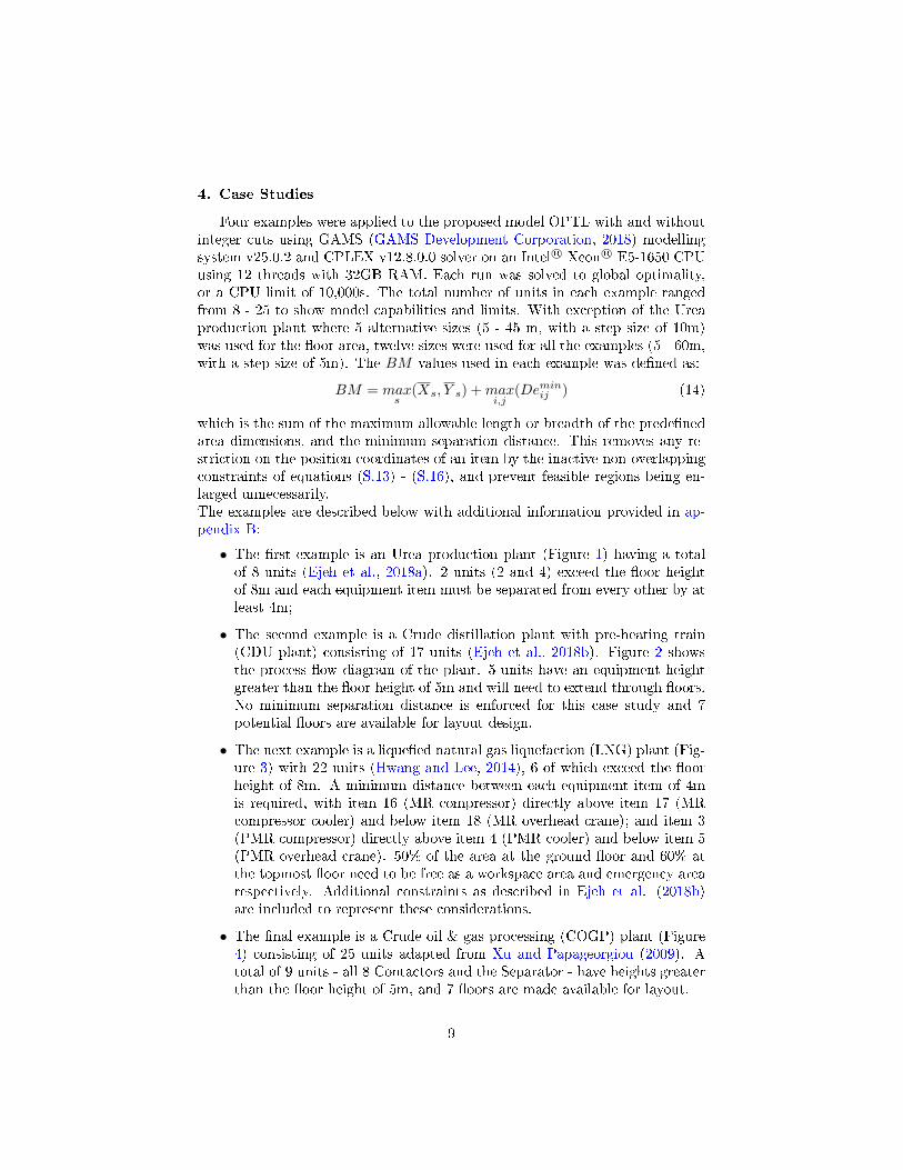
• The next example is a lique�ed natural gas liquefaction (LNG) plant (Fig-ure 3) with 22 units (Hwang and Lee, 2014), 6 of which exceed the �oorheight of 8m. A minimum distance between each equipment item of 4mis required, with item 16 (MR compressor) directly above item 17 (MRcompressor cooler) and below item 18 (MR overhead crane); and item 3(PMR compressor) directly above item 4 (PMR cooler) and below item 5(PMR overhead crane). 50% of the area at the ground �oor and 60% atthe topmost �oor need to be free as a workspace area and emergency arearespectively. Additional constraints as described in Ejeh et al. (2018b)are included to represent these considerations.

• The �nal example is a Crude oil & gas processing (COGP) plant (Figure4) consisting of 25 units adapted from Xu and Papageorgiou (2009). Atotal of 9 units - all 8 Contactors and the Separator - have heights greaterthan the �oor height of 5m, and 7 �oors are made available for layout.

9

Figure 1: Flow diagram of Urea Production Plant (See Table B.1 inAppendix B for a description of the equipment item label)

Figure 2: Flow diagram of Crude distillation (CDU) Plant (SeeTable B.3 in Appendix B for a description of the equipment item

label)

10

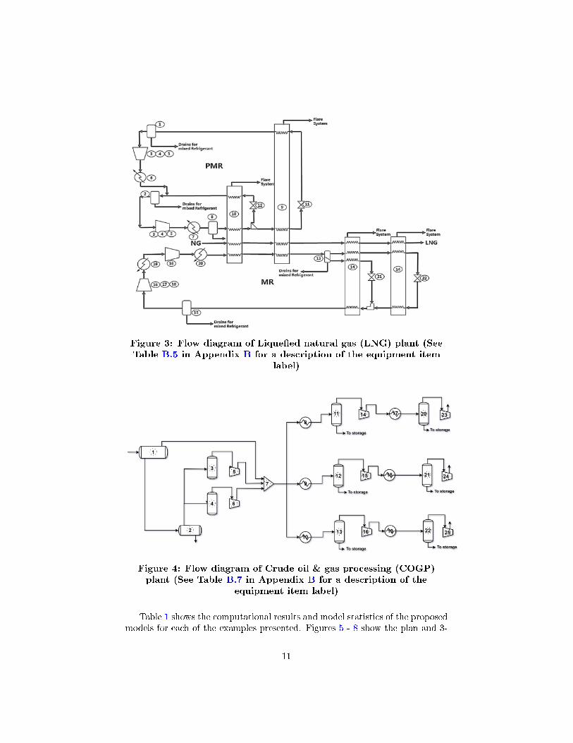
Figure 3: Flow diagram of Lique�ed natural gas (LNG) plant (SeeTable B.5 in Appendix B for a description of the equipment item

label)

Figure 4: Flow diagram of Crude oil & gas processing (COGP)plant (See Table B.7 in Appendix B for a description of the

equipment item label)

Table 1 shows the computational results and model statistics of the proposedmodels for each of the examples presented. Figures 5 - 8 show the plan and 3-

11

dimensional views of the optimal/best layouts obtained for each example. Eachof the 3D views are drawn from a direction that shows most of the equipmentitems for the case study being considered.

Table 1: Model Statistics & computational performance

Model Total Cost (rmu) CPU (s) Eqns1 Cts_var2 Dis_var3

Urea plant - 8 unitsOPTL 117,431.0 1.6 431 193 118OPTL_IC 117,431.0 0.6 543 193 118

CDU plant - 17 unitsOPTL 592,322.2 1,678.1 2,150 679 551OPTL_IC 592,322.2 131.6 3,102 679 551

LNG plant - 22 unitsOPTL 1,466,654.2 (2.8%)4 2,784 786 732OPTL_IC 1,466,654.2 (2.2%)4 4,786 786 732

COGP plant - 25 unitsOPTL 269,310.5 (17.0%)4 4,122 914 943OPTL_IC 255,320.4 (11.8%)4 7,022 914 943

1Eqns - No. of equations 2Cts_var - No. of continuous variables3Dis_var - No. of discrete variables 4Relative gap quoted at CPU limit of 10,000s

Relative gap (%) = |Best estimated solution − Best integer solution|max(Best estimated solution, Best integer solution)

× 100

The optimal layout for the Urea plant is shown in Figure 5. A total of 4�oors out of 4 made available were selected for the layout with an area of 5m× 15m and a total cost of 117,431.0 rmu. Units 2 and 4 each requiring 4 and 2�oors were positioned from the 1st and 2nd �oors respectively. This is consistentwith previously obtained results using Models A.1 - A.3 proposed by Ejeh et al.(2018a). However, the current model OPTL allows for additional �exibility tothe decision maker as the choice of the number of potential/available �oors canbe less than the number of �oors required by the tallest unit (4 �oors), which wasnot possible in the previous models. Table 2 shows a sensitivity analysis of theglobally optimal solution obtained by the current model OPTL and models A.1- A.3, to the number of �oors made available for layout in the Urea productionplant. Although the tallest unit 2 required 4 �oors, single �oor layout solutionscould still be obtained by model OPTL if required, unlike models A.1 - A.3. Amore informed decision can then be made on the compromise between the totalnumber of �oors and the total layout cost.

12

Table 2: Sensitivity analysis on the number of available �oors forUrea production plant

Available Model OPTL Models A.1 - A.3�oors, | K | NF Total Cost (rmu) NF Total Cost (rmu)

1 1 260,942.2 - -1

2 2 167,298.8 - -1

3 3 149,498.0 - -1

4 4 117,431.0 4 117,431.0

1Infeasible model

13

Figure 5: Optimal layout for Urea production plant

14

The layout results (plan and 3D view) for the CDU plant is shown in Figure6. A total of 7 �oors were selected with an area of 20m × 15m and a totalcost of 592,322.2 rmu. The total cost is about 2% less than the globally op-timal value obtained in previous models A.1 - A.3 in Ejeh et al. (2018b). Thiscost savings is majorly attributed to the fact that the proposed model allowsmulti-�oor equipment items extend well above the total number of �oors madeavailable and/or selected. Particularly, unit 6 requiring 4 �oors was assignedonly �oors 5, 6 and 7, and extended beyond the 7 available �oors. Table 3also shows the results of a sensitivity analysis on the number of available �oorsused in models OPTL and A.1 - A.3. In each of the cases shown, all modelswere solved to global optimality without a time restriction. The tallest unit inthe CDU example requires 5 �oors, hence models A.1 - A.3 could not solve theproblem for any number of available �oors less than 5. The proposed modelalso obtained the same or better solutions than previous models for each run.For 5 available �oors, although each of models OPTL and A.1 - A.3 selected 5total �oors, model OPTL obtained a smaller objective value than A.1 - A.3. Asimilar result was obtained with 6 and 7 available �oors. This was achieved byleveraging the feature where tall units were allowed by model OPTL to extendabove the �oors made available. This can bring about cost savings especiallywhere there are no restrictions to equipment �oor positions or the maximumheight of the process plant. The proposed model can also restrict equipmentpositioning only to the available number of �oors as in models A.1 - A.3. Thiscan be achieved by �xing the value of ωi to 0.

15

Figure 6: Best obtained layout for CDU plant

16

Table 3: Sensitivity analysis on the number of available �oors forCDU plant

Available Model OPTL Models A.1 - A.3�oors, | K | NF Total Cost (rmu) NF Total Cost (rmu)

1 1 1,112,094.7 - -1

2 2 855,465.8 - -1

3 3 697,672.4 - -1

4 4 624,452.8 - -1

5 5 603,886.5 5 614,820.06 5 603,886.5 5 614,820.07 7 592,322.2 5 603,886.5

1Infeasible model

The layout results of the much larger chemical plants - LNG and COGP- having 22 and 25 units are shown in Figures 7 and 8 respectively. For theLNG plant, a total cost of 1,466,654.2 rmu was obtained with 5 �oors selectedmeasuring 35m × 30m. None of the multi-�oor equipment items extended wellabove the top-most �oor and all additional considerations for the plant wereaddressed in the solution obtained. A total cost of 269,310.5 rmu was realisedfor the COGP plant having 7 �oors with a �oor are of 20m × 10m.

17

Figure 7: Best obtained layout for LNG plant

18

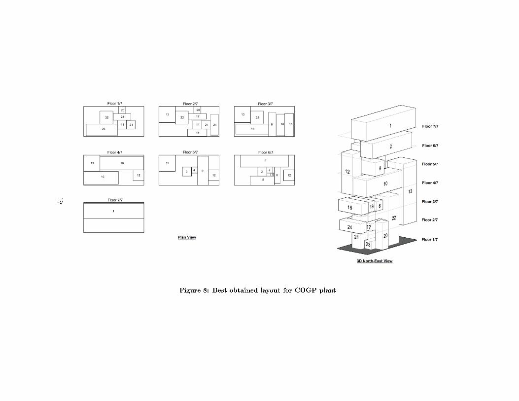
Figure 8: Best obtained layout for COGP plant

19

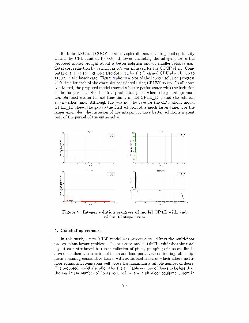
Both the LNG and COGP plant examples did not solve to global optimalitywithin the CPU limit of 10,000s. However, including the integer cuts to theproposed model brought about a better solution and/or smaller relative gap.Total cost reduction by as much as 5% was achieved for the COGP plant. Com-putational time savings were also obtained for the Urea and CDU plant by up to1100% in the latter case. Figure 9 shows a plot of the integer solution progresswith time for each of the examples considered using CPLEX solver. In all casesconsidered, the proposed model showed a better performance with the inclusionof the integer cut. For the Urea production plant where the global optimumwas obtained within the set time limit, model OPTL_IC found the solutionat an earlier time. Although this was not the case for the CDU plant, modelOPTL_IC closed the gap to the �nal solution at a much faster time. For thelarger examples, the inclusion of the integer cut gave better solutions a greatpart of the period of the entire solve.

Figure 9: Integer solution progress of model OPTL with andwithout integer cuts

5. Concluding remarks

In this work, a new MILP model was proposed to address the multi-�oorprocess plant layout problem. The proposed model, OPTL, minimises the totallayout cost attributed to the installation of pipes, pumping of process �uids,area-dependent construction of �oors and land purchase, considering tall equip-ment spanning consecutive �oors, with additional features which allows multi-�oor equipment items span well above the maximum available number of �oors.The proposed model also allows for the available number of �oors to be less thanthe maximum number of �oors required by any multi-�oor equipment item in

20

the plant. Integer cuts were further included to improve the computational ef-�ciency of the model by eliminating unrealistic layout scenarios and restrictingcertain binary variable values. Model computational performance and limitswere demonstrated with four industry-relevant case studies having a total of 8- 25 units, and results compared with existing multi-�oor layout models withsimilar considerations (Ejeh et al., 2018a;b). The case studies included an 8-unit Urea production plant, a 17-unit crude distillation (CDU) plant, a lique�ednatural gas (LNG) plant having 22 units and a Crude oil & gas processing plantwith 25 units. Each of these plants had units with height greater than thestandard �oor height for each plant.Results showed that model OPTL successfully handled the unique layout con-siderations of each case study. The proposed model was able to achieve sameor better solution than previously obtained from other models. It also presen-ted more layout solution options to the decision maker based on the choiceof the number of �oors available. The inclusion of the integer cuts in modelOPTL showed improvements on the solutions obtained, CPU and/or relativegap achieved at the set time limit in all examples considered.Further work still needs to be carried out especially on alternative solutionmethods for larger examples similar to the construction-based approach (Xu andPapageorgiou, 2007) and the improvement-type algorithm (Xu and Papageor-giou, 2009). As a future work, solution algorithms will be investigated to obtainoptimal solutions in reasonable computational times.

Acknowledgement

JOE gratefully acknowledges the Petroleum Technology Development Fund(PTDF), Nigeria.

21

Appendix A. MILP models for multi-�oor process plant layout

Models A.1 - A.3 proposed by Ejeh et al. (2018b) for cases without produc-tion sections are presented as follows:

A.1. Model A.1

A.1.1. Floor constraints

Floor constraints ensure that equipment items are assigned to an equivalentnumber of �oors based on their height and that a �oor exists only if an equipmentitem is placed on it: ∑

k

Vik =Mi ∀ i (S.1)

Nij ≥ Vik + Vjk − 1 ∀ i, j > i (S.2)

Ssik ≤Wk ∀ i, k (S.3)

Wk ≤Wk−1 ∀ k > 1; (S.4)

NF ≥∑k

Wk ∀ i (S.5)

A.1.2. Equipment orientation constraints

A 900 rotation of equipment orientation is allowed in the x-y plane.

li = αiOi + βi(1−Oi) ∀ i (S.6)

di = αi + βi − li ∀ i (S.7)

A.1.3. Multi-�oor equipment constraints

Multi-�oor equipment is modelled as follows:

−Vik + Vi,k−1 + Ssik ≥ 0 ∀i, k (S.8)

−Vik + Vi,k+1 + Sfik ≥ 0 ∀i, k (S.9)∑k

Ssik = 1 ∀i (S.10)∑k

Sfik = 1 ∀i (S.11)

k′+Mi−1∑k=k′

Vik′ ≥Mi.Ssik ∀i, k (S.12)

22

A.1.4. Non-overlapping constraints

To prevent two or more equipment items occupying the same space withina �oor, the following constraints are introduced:

xi − xj +BM(1−Nij + E1ij + E2ij) ≥li + lj

2+Deminij ∀ i, j > i (S.13)

xj − xi +BM(2−Nij − E1ij + E2ij) ≥li + lj


yi − yj +BM(2−Nij + E1ij − E2ij) ≥di + dj


yj − yi +BM(3−Nij − E1ij − E2ij) ≥di + dj


A.1.5. Distance constraints

Distance constraints determine the relative distances in the x and y coordin-ates between connected equipment.

Rij − Lij = xi − xj ∀ i, j : fij = 1 (S.17)

Aij −Bij = yi − yj ∀ i, j : fij = 1 (S.18)

Uij −Dij = FH∑k

(k − 1)(Ssik − Ssjk) + OPij − IPij ∀ i, j : fij = 1

(S.19)

TDij = Rij + Lij +Aij +Bij + Uij +Dij ∀ i, j : fij = 1 (S.20)

A.1.6. Area Constraints

The area of each �oor is as described by equations (S.21) - (S.26).

FA =∑s

ARsQs (S.21)∑s

Qs = 1 (S.22)

The �oor length and depth is selected from the chosen rectangular area sizedimensions:

Xmax =∑s

XsQs (S.23)

Y max =∑s

Y sQs (S.24)

NQs ≤ K ·Qs ∀s (S.25)

NF =∑s

NQs (S.26)

23

A.1.7. Layout design constraints

Layout design constraints ensure that equipment items are placed within theboundaries of the �oor area and start from the base of a �oor.

xi ≥li2

∀ i (S.27)

yi ≥di2

∀ i (S.28)

xi +li2≤ Xmax ∀ i (S.29)

yi +di2≤ Y max ∀ i (S.30)

A.1.8. Symmetry breaking constraints

Symmetry breaking constraints are introduced as follows:

xi + yi − xj − yj ≥ δ ·Nij ∀ (i, j) = argmaxi,j∈MF

Ccij (S.31)

E1ij = 0 ∀ (i, j) = argmaxi,j∈MF

Ccij (S.32)

where δ = min(li2 ,

di2

)+ min

(lj2 ,

dj2

). These �x the relative position of i to

j. Units i and j are chosen as the two multi-�oor units having the highestconnection costs.

A.1.9. Objective function

min∑i

∑j 6=i:fij=1

[CcijTDij + CvijDij + Chij(Rij + Lij +Aij +Bij)]

+FC1 ·NF + FC2∑s

ARs ·NQs + LC · FA(S.33)

subject to (S.1) - (S.32).

A.2. Model A.2

Model A.2 has the same formulation as A.1 with the exception that equations(S.9), (S.11) and (S.12) are replaced by (S.34) below:

Mi−1∑θ=1

Vi,k+θ ≥ (M i − 1).(Vik − Vi,k−1) ∀i, k (S.34)

A.3. Model A.3

For Model A.3, equations (S.8), (S.9) and (S.12) in model A.1 are replacedby (S.35) below:

Vik − Vi,k−1 = Ssik − Sfi,k−1 ∀i, k (S.35)

24

Appendix B. Data for case studies

B.1. Urea production plant

The dimensions of equipment items in the Urea plant are given in Table B.1.Table B.2 shows the connection cost, connection heights, horizontal and verticalpumping costs, as well as other required data.

Table B.1: Equipment dimensions for the Urea production plant

EquipmentDescription αi(m) βi(m) γi(m)item

1 Flash drum 1.9812 1.9812 6.09602 Reactor 1 2.4384 2.4384 28.9563 Reactor 2 1.5240 1.5240 5.79124 Distillation Column 1 1.0668 1.0668 14.63045 Distillation Column 2 0.6096 0.6096 7.31526 Reactor 3 0.7620 0.7620 3.35287 Reactor 4 1.2192 1.2192 5.02928 Separator 1.0668 1.0668 3.6576

Table B.2: Parameters for the Urea production plant

(a) Connection and pumping costs, and connection heights

Connection Ccij(rmu/m) Chij(rmu/m) Cvij(rmu/m) OPij(m) IPij(m)

1.4 38.0 662.2 6621.8 0.0000 12.80164.3 161.0 513.3 5133.4 14.6304 4.63304.7 25.0 332.2 3321.8 0.0000 1.00587.8 25.0 332.2 3321.8 1.0058 2.92613.2 124.0 803.5 8035.1 1.1582 0.00002.1 103.0 803.5 8035.1 28.9560 4.57201.5 62.0 141.3 1413.3 6.0960 1.82888.6 14.0 59.0 590.0 3.6576 3.35286.5 13.0 59.0 590.0 3.3528 5.48645.3 17.0 156.2 1561.7 0.0000 4.6330

(b) Other Parameters

Parameters Value| K | 4FC1(rmu) 3,200FC2 (rmu/m2) 120LC (rmu/m2) 420FH (m) 8.0

25

B.2. Crude distillation plant with pre-heating train (CDU) plant)

The dimensions of equipment items in the CDU plant are given in TableB.3. Table B.4 shows the connection cost, connection heights, horizontal andvertical pumping costs, as well as other required data.

Table B.3: Equipment dimensions for the CDU plant


1 Crude preheater 1 6.000 0.974 0.9742 Crude preheater 2 2.550 0.620 0.6203 Desalter 5.572 3.715 3.7154 Pre�ash heater 2.550 0.774 0.7745 Pre�ash drum 5.251 5.251 7.8776 Fired heater (CDU) 3.922 3.922 17.6007 Crude distillation tower 12.300 12.300 14.5008 Naphtha condenser 1.789 1.193 1.1939 Kerosene SS 1.500 1.500 3.90010 Diesel SS 1.500 1.500 3.90011 AGO SS 1.500 1.500 3.90012 Fired heater (VDU) 3.922 3.922 17.60013 Vacuum distillation tower 9.410 9.410 4.50014 Kerosene reboiler 3.050 2.033 2.03315 Debutaniser 5.337 5.337 24.75016 Stabilised Naphtha condenser 1.789 1.193 1.19317 Debutaniser reboiler 1.789 1.193 1.193

26

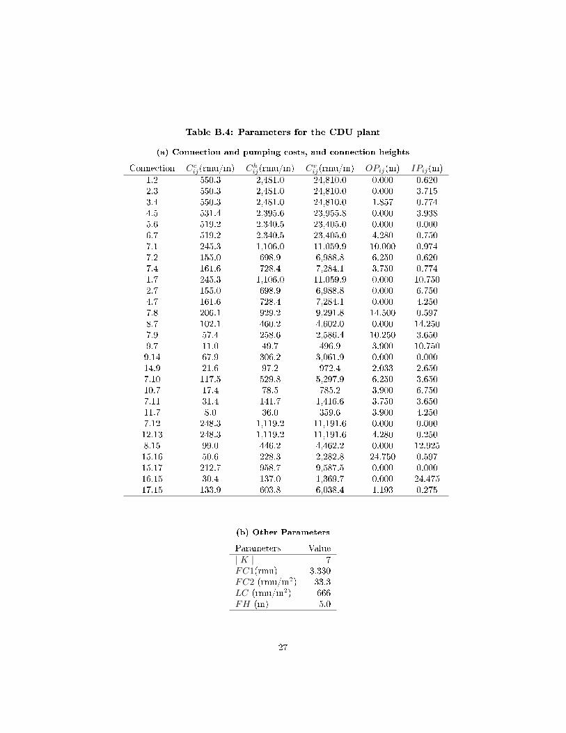
Table B.4: Parameters for the CDU plant



1.2 550.3 2,481.0 24,810.0 0.000 0.6202.3 550.3 2,481.0 24,810.0 0.000 3.7153.4 550.3 2,481.0 24,810.0 1.857 0.7744.5 531.4 2,395.6 23,955.8 0.000 3.9385.6 519.2 2,340.5 23,405.0 0.000 0.0006.7 519.2 2,340.5 23,405.0 4.280 0.7507.1 245.3 1,106.0 11,059.9 10.000 0.9747.2 155.0 698.9 6,988.8 6.250 0.6207.4 161.6 728.4 7,284.1 3.750 0.7741.7 245.3 1,106.0 11,059.9 0.000 10.7502.7 155.0 698.9 6,988.8 0.000 6.7504.7 161.6 728.4 7,284.1 0.000 4.2507.8 206.1 929.2 9,291.8 14.500 0.5978.7 102.1 460.2 4,602.0 0.000 14.2507.9 57.4 258.6 2,586.4 10.250 3.6509.7 11.0 49.7 496.9 3.900 10.7509.14 67.9 306.2 3,061.9 0.000 0.00014.9 21.6 97.2 972.4 2.033 2.6507.10 117.5 529.8 5,297.9 6.250 3.65010.7 17.4 78.5 785.2 3.900 6.7507.11 31.4 141.7 1,416.6 3.750 3.65011.7 8.0 36.0 359.6 3.900 4.2507.12 248.3 1,119.2 11,191.6 0.000 0.00012.13 248.3 1,119.2 11,191.6 4.280 0.2508.15 99.0 446.2 4,462.2 0.000 12.92515.16 50.6 228.3 2,282.8 24.750 0.59715.17 212.7 958.7 9,587.5 0.000 0.00016.15 30.4 137.0 1,369.7 0.000 24.47517.15 133.9 603.8 6,038.4 1.193 0.275


Parameters Value| K | 7FC1(rmu) 3,330FC2 (rmu/m2) 33.3LC (rmu/m2) 666FH (m) 5.0

27

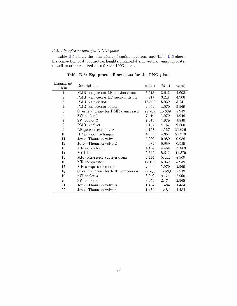
B.3. Lique�ed natural gas (LNG) plant

Table B.5 shows the dimensions of equipment items and Table B.6 showsthe connection cost, connection heights, horizontal and vertical pumping costs,as well as other required data for the LNG plant.

Table B.5: Equipment dimensions for the LNG plant


1 PMR compressor LP suction drum 3.613 3.613 4.6032 PMR compressor HP suction drum 3.217 3.217 4.9003 PMR compressor 18.809 5.939 5.7414 PMR compressor cooler 2.969 1.979 2.9695 Overhead crane for PMR compressor 22.769 15.839 5.9396 SW cooler 1 7.919 1.979 4.9497 SW cooler 2 7.919 1.979 4.9498 PMR receiver 4.157 4.157 9.8009 LP precool exchanger 4.157 4.157 21.08610 HP precool exchanger 4.355 4.355 21.77911 Joule�Thomson valve 1 0.989 0.989 0.98912 Joule�Thomson valve 2 0.989 0.989 0.98913 MR separator 1 4.454 4.454 12.86914 MCHE 5.642 5.642 41.57915 MR compressor suction drum 5.444 5.444 8.90916 MR compressor 17.126 5.939 5.93917 MR compressor cooler 2.969 1.979 2.96918 Overhead crane for MR Compressor 22.769 15.839 5.93919 SW cooler 3 3.959 2.474 2.96920 SW cooler 4 3.959 2.474 2.96921 Joule�Thomson valve 3 1.484 1.484 1.48422 Joule�Thomson valve 4 1.484 1.484 1.484

28

Table B.6: Parameters for the LNG plant



2.3 150 750 7500 2.4500 2.87053.6 150 750 7500 2.8705 2.47453.7 150 750 7500 2.8705 2.47457.2 150 750 7500 2.4745 2.45008.10 150 750 7500 8.9000 4.000010.11 150 750 7500 18.8895 0.494511.10 150 750 7500 0.4945 18.88959.10 150 750 7500 4.0000 18.889510.9 150 750 7500 18.8598 4.000012.9 70 250 2500 0.4945 18.54309.12 70 250 2500 18.4530 0.494513.14 150 750 7500 4.0000 12.000014.15 150 750 7500 4.0000 4.000015.16 150 750 7500 8.4545 2.969516.17 150 750 7500 2.9795 1.484517.16 150 750 7500 1.4845 2.969514.21 70 250 2500 28.0000 0.742021.14 70 250 2500 0.7420 28.000016.19 150 750 7500 2.9695 1.484519.16 150 750 7500 1.4845 2.969516.20 150 750 7500 2.9695 1.484520.16 150 750 7500 1.4845 2.969522.14 150 750 7500 0.7420 36.789514.22 150 750 7500 36.7895 0.742010.2 150 750 7500 12.0000 2.45009.1 150 750 7500 12.0000 2.30156.8 150 750 7500 2.4745 8.900014.9 150 750 7500 20.0000 12.000010.13 150 750 7500 4.0000 4.0000



29

B.4. Crude oil & gas processing (COGP) plant

Table B.7 shows the dimensions of equipment items and Table B.8 showsthe connection cost, connection heights, horizontal and vertical pumping costs,as well as other required data for the COGP plant.

Table B.7: Equipment dimensions for the COGP plant


1 Separator 20.000 5.000 5.0002 KO drum 16.000 4.000 4.0003 Contactor 1 3.000 3.000 8.0004 Contactor 2 2.000 2.000 5.3335 Compressor 1 8.000 3.000 3.0006 Compressor 2 5.333 2.000 2.0007 Mixer 1 1.000 1.000 1.0008 Heat exchanger 1 8.000 2.500 2.5009 Heat exchanger 2 9.600 3.600 3.60010 Heat exchanger 3 14.400 4.500 4.50011 Contactor 3 3.000 3.000 9.00012 Contactor 4 3.600 3.600 10.80013 Contactor 5 5.400 5.400 16.20014 Compressor 3 6.400 2.400 2.40015 Compressor 4 7.680 2.880 2.88016 Compressor 5 11.520 4.320 4.32017 Heat exchanger 4 6.000 1.875 1.87518 Heat exchanger 5 7.200 2.700 2.70019 Heat exchanger 6 10.800 3.375 3.37520 Contactor 6 2.400 2.400 7.20021 Contactor 7 2.880 2.880 8.64022 Contactor 8 4.320 4.320 12.96023 Compressor 6 5.760 2.160 2.16024 Compressor 7 6.912 2.592 2.59225 Compressor 8 10.368 3.888 3.888

30

Table B.8: Parameters for the COGP plant



1.7 50.00 225.00 2250.0 0.000 1.0001.2 200.00 900.00 9000.0 0.000 2.0002.4 72.00 324.00 3240.0 0.000 2.6674.6 72.00 324.00 3240.0 5.333 2.0006.7 72.00 324.00 3240.0 2.000 1.0005.7 108.00 486.00 4860.0 3.000 1.0002.3 108.00 486.00 4860.0 0.000 4.0003.5 108.00 486.00 4860.0 8.000 3.0007.8 57.50 258.75 2587.5 0.000 2.5007.9 69.00 310.50 3105.0 0.000 3.6007.10 103.50 465.75 4657.5 0.000 4.5008.11 57.50 258.75 2587.5 0.000 4.50011.14 46.00 207.00 2070.0 9.000 2.40014.17 46.00 207.00 2070.0 2.400 1.87517.20 46.00 207.00 2070.0 0.000 3.60020.23 41.40 186.30 1863.0 7.200 2.1609.12 69.00 310.50 3105.0 0.000 5.40012.15 55.20 248.40 2484.0 10.800 2.88015.18 55.20 248.40 2484.0 2.880 2.70018.21 55.20 248.40 2484.0 0.000 4.32021.24 49.68 223.56 2235.6 8.640 2.59210.13 103.50 465.75 4657.5 0.000 8.10013.16 82.80 372.60 3726.0 16.200 4.32016.19 82.80 372.60 3726.0 4.320 3.37519.22 82.80 372.60 3726.0 0.000 6.48022.25 74.52 335.34 3353.4 12.960 3.888



31

References

American Institute of Chemical Engineers, 1994. Dow's �re & explosion indexhazard classi�cation guide. Vol. 7. John Wiley & Sons, Inc., Hoboken, NJ,USA.

Barbosa-Póvoa, A. P., Mateus, R., Novais, A. Q., 2002. Optimal 3D layout ofindustrial facilities. Int. J. Prod. Res. 40, 1669�1698.

Brunoro Ahumada, C., Quddus, N., Mannan, M. S., 2018. A method for facilitylayout optimisation including stochastic risk assessment. Process Saf. Environ.Prot. 117, 616�628.

de Lira-Flores, J., Vázquez-Román, R., López-Molina, A., Mannan, M. S., 2014.A MINLP approach for layout designs based on the domino hazard index. J.Loss Prev. Process Ind. 30, 219�227.

Ejeh, J. O., Liu, S., Chalchooghi, M. M., Papageorgiou, L. G., 2018a.Optimization-based approach for process plant layout. Ind. Eng. Chem. Res.57, 10482�10490.

Ejeh, J. O., Liu, S., Papageorgiou, L. G., 2018b. Optimal multi-�oor processplant layout with production sections. Chem. Eng. Res. Des. 137, 488�501.

Furuholmen, M., Glette, K., Hovin, M., Torresen, J., 2010. A coevolutionary,hyper heuristic approach to the optimization of three-dimensional processplant layouts - A comparative study. In: IEEE Congress on EvolutionaryComputation. IEEE, pp. 1�8.

GAMS Development Corporation, 2018. General algebraic modeling system(GAMS) release 25.0.2.

Georgiadis, M., Macchietto, S., 1997. Layout of process plants: A novel ap-proach. Comput. Chem. Eng. 21, S337�S342.

Guirardello, R., Swaney, R. E., 2005. Optimization of process plant layout withpipe routing. Comput. Chem. Eng. 30, 99�114.

Hosseini-Nasab, H., Fereidouni, S., Fatemi Ghomi, S. M. T., Fakhrzad, M. B.,2018. Classi�cation of facility layout problems: a review study. Int. J. Adv.Manuf. Technol. 94, 957�977.

Hwang, J., Lee, K. Y., 2014. Optimal liquefaction process cycle considering sim-plicity and e�ciency for LNG FPSO at FEED stage. Computers and ChemicalEngineering 63, 1�33.

Kheirkhah, A., Navidi, H., Messi Bidgoli, M., 2015. Dynamic facility layoutproblem: a new bilevel formulation and some metaheuristic solution methods.IEEE Trans. Eng. Manag. 62, 396�410.

32

Kondili, E., Pantelides, C. C., Sargent, R. W. H., 1993. A general algorithmfor short-term scheduling of batch operations-I. MILP formulation. Comput.Chem. Eng. 17, 211�227.

López-Molina, A., Vázquez-Román, R., Mannan, M. S., Félix-Flores, M. G.,2013. An approach for domino e�ect reduction based on optimal layouts. J.Loss Prev. Process Ind. 26, 887�894.

Moran, S., 2017. Process plant layout, 2nd Edition. Butterworth-Heinemann.

Nabavi, S., Taghipour, A., Mohammadpour Gorji, A., 2016. Optimization offacility layout of tank farms using genetic algorithm and �reball scenario.Chem. Prod. Process Model. 11, 149�157.

Papageorgiou, L. G., Rotstein, G. E., 1998. Continuous-domain mathematicalmodels for optimal process plant layout. Ind. Eng. Chem. Res. 37, 3631�3639.

Park, P. J., Lee, C. J., 2015. The research of optimal plant layout optimizationbased on particle swarm optimization for ethylene oxide plant. J. Korean Soc.Saf. 30, 32�37.

Patsiatzis, D. I., Knight, G., Papageorgiou, L. G., 2004. An MILP approach tosafe process plant layout. Chem. Eng. Res. Des. 82, 579�586.

Patsiatzis, D. I., Papageorgiou, L. G., 2002. Optimal multi-�oor process plantlayout. Comput. Chem. Eng. 26, 575�583.

Patsiatzis, D. I., Papageorgiou, L. G., 2003. E�cient solution approaches for themulti�oor process plant layout problem. Ind. Eng. Chem. Res. 42, 811�824.

Patsiatzis, D. I., Xu, G., Papageorgiou, L. G., 2005. Layout aspects of pipelessbatch plants. Ind. Eng. Chem. Res. 44, 5672�5679.

Penteado, F. D., Ciric, A. R., 1996. An MINLP approach for safe process plantlayout. Ind. Eng. Chem. Res. 35, 1354�1361.

Tugnoli, A., Khan, F., Amyotte, P., Cozzani, V., 2008. Safety assessment inplant layout design using indexing approach: Implementing inherent safetyperspective. Part 2-Domino Hazard Index and case study. J. Hazard. Mater.160, 110�121.

Xu, G., Papageorgiou, L. G., 2007. A construction-based approach to processplant layout using mixed-integer optimization. Ind. Eng. Chem. Res. 46, 351�358.

Xu, G., Papageorgiou, L. G., 2009. Process plant layout using an improvement-type algorithm. Chem. Eng. Res. Des. 87, 780�788.

33

optimal layout of multi-floor process plants using milp

Documents