a mathematical biologist’s guide to absolute and

Bull Math Biol (2014) 76:1–26DOI 10.1007/s11538-013-9911-9

R E V I E W A RT I C L E

A Mathematical Biologist’s Guide to Absoluteand Convective Instability

Jonathan A. Sherratt · Ayawoa S. Dagbovie ·Frank M. Hilker

Received: 29 June 2013 / Accepted: 8 October 2013 / Published online: 22 November 2013© Society for Mathematical Biology 2013

Abstract Mathematical models have been highly successful at reproducing the com-plex spatiotemporal phenomena seen in many biological systems. However, the abil-ity to numerically simulate such phenomena currently far outstrips detailed math-ematical understanding. This paper reviews the theory of absolute and convectiveinstability, which has the potential to redress this inbalance in some cases. In spa-tiotemporal systems, unstable steady states subdivide into two categories. Those thatare absolutely unstable are not relevant in applications except as generators of spa-tial or spatiotemporal patterns, but convectively unstable steady states can occur aspersistent features of solutions. The authors explain the concepts of absolute and con-vective instability, and also the related concepts of remnant and transient instability.They give examples of their use in explaining qualitative transitions in solution be-haviour. They then describe how to distinguish different types of instability, focussingon the relatively new approach of the absolute spectrum. They also discuss the useof the theory for making quantitative predictions on how spatiotemporal solutionschange with model parameters. The discussion is illustrated throughout by numericalsimulations of a model for river-based predator–prey systems.

Keywords Absolute stability · Partial differential equations · Pattern formation ·Spatiotemporal patterns · Review · Survey

J.A. Sherratt (B) · A.S. DagbovieDepartment of Mathematics and Maxwell Institute for Mathematical Sciences, Heriot-WattUniversity, Edinburgh EH14 4AS, UKe-mail: [email protected]

A.S. Dagboviee-mail: [email protected]

F.M. HilkerCentre for Mathematical Biology and Department of Mathematical Sciences, University of Bath,Bath BA2 7AY, UKe-mail: [email protected]

mailto:[email protected]



2 J.A. Sherratt et al.

1 Introduction

Almost all undergraduate courses in mathematical biology include a section on ordi-nary differential equation (ODE) models. The central player in the course material isthe stability of steady states. Students learn that only (locally) stable steady states arebiologically significant. Later in their careers, students are introduced to partial dif-ferential equation (PDE) models. Again, the stability of (homogeneous) steady statesplays a central role. In particular, the first exposure that many students receive to bi-ological pattern formation is the Turing mechanism, in which a homogeneous steadystate that is stable in the kinetic ODEs is destabilised by the addition of diffusionterms. However, steady states that are unstable in the kinetic ODEs are almost nevermentioned. As a result, there is a widespread assumption that unstable steady statesare not biologically significant as PDE solutions. This is not true. In fact, such steadystates fall into one of two categories. If they are “absolutely unstable”, then theyare indeed not biologically significant, except perhaps as providing the mathematicalorigin of spatial or spatiotemporal patterns. But “convectively unstable” steady statescan be an important and persistent feature of PDE solutions. The objective of this pa-per is to explain the concepts of absolute and convective instability and the relatedconcepts of remnant and transient instability, to illustrate their implications for PDE

models of biological systems, and to summarise methods for distinguishing differenttypes of instability in practice.

We begin with an illustrative example: the invasion of a prey population by preda-tors. This problem has been addressed in many modelling studies. Simple invasionscorrespond to a standard transition front (e.g. Owen and Lewis 2001), but there isnow a considerable body of work on invasions that leave more complex spatiotempo-ral phenomena in their wake: see, for example, Sherratt et al. (1995), Petrovskii andMalchow (2000), Morozov et al. (2006), Merchant and Nagata (2010, 2011). We willfocus on the spatially extended Rosenzweig–MacArthur (1963) model for predator–prey interaction, and for clarity all of the numerical simulations in this paper will usethis model. We give the equations in a dimensionless form:

predators∂p

∂t=

dispersal︷︸︸︷

d∂2p

∂x2+

advection︷︸︸︷

c∂p

∂x+

benefit frompredation

︷︸︸︷

(μ/b)hp/(1 + μh)−death︷︸︸︷

p/ab, (1a)

prey∂h

∂t= ∂2h

∂x2︸︷︷︸

dispersal

+ c∂h

∂x︸︷︷︸

advection

+ h(1 − h)︸︷︷︸

intrinsicbirth and death

− μph

1 + μh︸︷︷︸

predation

. (1b)

Here, p and h denote predator and prey densities, which depend on space x andtime t . Here, and throughout this paper, we restrict attention to one space dimension:The theory of absolute stability is not yet fully developed in higher dimensions. Mostpredator–prey studies do not include advection terms, but allowing c �= 0 enables aclearer illustration of some of the concepts we will be discussing. Advection of thistype arises naturally in river-based predator–prey systems (Hilker and Lewis 2010).The prey consumption rate per predator is an increasing saturating function of the

A Guide to Absolute and Convective Instability 3

Fig. 1 Numerical simulation of predators invading prey using the Rosenzweig–MacArthur (1963) model(1a), (1b) without advection. At time t = 0, the system was in the prey-only steady state (1,0) except fora small predator density near the left-hand boundary. The solution is plotted at t = 4000. In (a), the pa-rameters are such that the coexistence steady state is stable, and the invasion consists of a simple transitionfront, connecting the prey-only state and the coexistence state. In (b), the coexistence state persists in aplateau behind the leading front, with spatiotemporal oscillations further back. In (c) there is a periodictravelling wave immediately behind and moving at the same speed as the leading front, with more irregularoscillations further back. Note that for Eq. (1a), (1b), the existence of both steady state to steady state andsteady state to wavetrain transition fronts has been proved by Dunbar (1986) in the limit as d → ∞, withextensions to d finite and sufficiently large by Fraile and Sabina (1989) in the latter case. The parametervalues were a = 1.3, b = 4, c = 0, d = 2 and (a) μ = 7; (b) μ = 8; (c) μ = 9. The equations were solvednumerically using a semi-implicit finite difference method with a grid spacing of 0.5 and a time step of0.01. We solved on the domain 0 < x < 2500, with zero flux conditions px = hx = 0 at both boundaries

prey density with Holling type II form: μ > 0 reflects how quickly the consumptionrate saturates as prey density increases. Parameters a > 0 and b > 0 are dimensionlesscombinations of the birth and death rates; Details of the nondimensionalisation aregiven in Appendix A of Smith et al. (2008), and in many textbooks. The parameterd > 0 is the ratio of predator to prey dispersal coefficients. The value of d will besignificantly greater than one for most mammalian systems (e.g. Brandt and Lambin2007) and also for macroscopic marine species (Wieters et al. 2008). However, d willtypically be closer to one for aquatic microorganisms (Hauzy et al. 2007). Provideda > 1 + 1/μ, Eqs. (1a), (1b) have a unique homogeneous coexistence steady state(hs,ps) where hs = 1/(aμ − μ) and ps = (1 − hs)(1 + μhs)/μ, which is stable as asolution of the kinetic ODEs only if μ < μcrit = (a + 1)/(a − 1).

Figure 1 illustrates simulations of the invasion of a prey population by predatorsusing (1a), (1b) with no advection, i.e. c = 0. For μ < μcrit, invasion takes the formof a simple transition wave, with the prey-only state (1,0) ahead of the wave andthe stable coexistence state (hs,ps) behind it (see Fig. 1a). But as μ is increasedabove μcrit, so that the coexistence steady state becomes unstable, this steady state


does not suddenly disappear (see Fig. 1b, c). Rather, for a range of μ values aboveμcrit there is plateau behind the front in which the solution is at the coexistence state,with spatiotemporal oscillations further back. This plateau is a persistent feature ofthe invasion profile, despite the fact that the coexistence steady state is unstable. Mal-chow and Petrovskii (2002) termed this phenomenon “dynamical stabilization”, andthe key to understanding it is the concept of absolute vs. convective instability. InSect. 2, we explain these terms, and in Sect. 3 we give an example of their use inexplaining qualitative transitions in solution behaviour. In Sect. 4, we summarisethe historical development of the theory, and in Sect. 5 we describe how to distin-guish different types of instability using the relatively new approach of the “absolutespectrum”. In Sect. 6, we explain how the theory can be used to make quantitativepredictions on how aspects of spatiotemporal behaviour change with model param-eters. In Sect. 7, we summarise our discussion, consider its application to a widerclass of solutions and place the concept of convective and absolute instabilities intothe context of ecology, especially with respect to perturbations in stream ecosystemsand biological pattern formation.

2 Absolute and Convective Stability

In a temporal system, stability is a relatively simple concept: A solution is (lo-cally) stable if any small perturbation decays. The same is true in a spatiotem-poral system: An unstable steady state is defined as one for which some smallperturbations grow over time. However, the situation is complicated by the factthat spatially localised perturbations may move while they are growing. Conse-quently, it is possible that a perturbation may decay at the location at which itis applied, even though it is growing overall (Fig. 2a, b). “Convective instabil-ity” occurs when all growing perturbations (linear modes) move while they are

Fig. 2 A schematic illustration of different types of instability. (a) In transient convective instability, allunstable linear modes move in a single direction while they are growing. (b) In non-transient convectiveinstability, all unstable linear modes move while they are growing, but in both directions. (c) In absoluteinstability, there is a stationary unstable linear mode, so that there are perturbations that grow at the locationat which they are applied. The figure is adapted from Fig. 1 of Sandstede and Scheel (2000b)


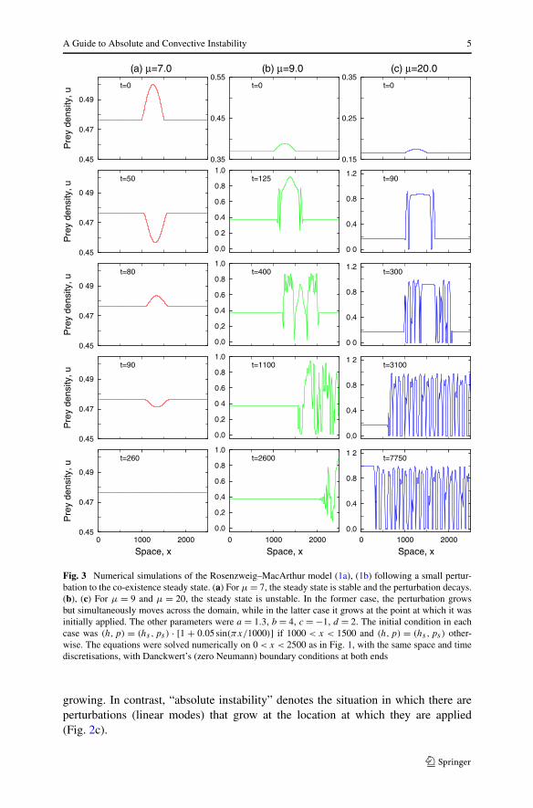
Fig. 3 Numerical simulations of the Rosenzweig–MacArthur model (1a), (1b) following a small pertur-bation to the co-existence steady state. (a) For μ = 7, the steady state is stable and the perturbation decays.(b), (c) For μ = 9 and μ = 20, the steady state is unstable. In the former case, the perturbation growsbut simultaneously moves across the domain, while in the latter case it grows at the point at which it wasinitially applied. The other parameters were a = 1.3, b = 4, c = −1, d = 2. The initial condition in eachcase was (h,p) = (hs ,ps) · [1 + 0.05 sin(πx/1000)] if 1000 < x < 1500 and (h,p) = (hs ,ps) other-wise. The equations were solved numerically on 0 < x < 2500 as in Fig. 1, with the same space and timediscretisations, with Danckwert’s (zero Neumann) boundary conditions at both ends

growing. In contrast, “absolute instability” denotes the situation in which there areperturbations (linear modes) that grow at the location at which they are applied(Fig. 2c).


In Fig. 3, we illustrate these two types of instability using simulations of (1a),(1b). We apply a small perturbation, localised around the centre of the domain, to thecoexistence steady state (hs,ps). For μ < μcrit = 7.67, the steady state is stable andthe perturbation decays. For μ = 9, the perturbation grows but moves in the positivex direction, decaying at its original location, while for μ = 20 the perturbation growsat its original location. This illustrates the fact that for the values of a, b, c, and d

used in the figure, the coexistence steady state is convectively unstable for μ = 9 andabsolutely unstable for μ = 20. Note that our choice of μ as a control parameter isessentially arbitrary, and similar changes can be induced by changes in a, b, c, or d ,for appropriate values of the other parameters.

Practical applications of PDE models in mathematical biology almost always occuron finite domains, and then boundary conditions must be considered when drawingconclusions about stability. If one considers (1a), (1b) on a domain with periodicboundary conditions, and with a value of μ giving convective instability, a movinggrowing perturbation will eventually reach the right-hand boundary. It will then re-enter at the left-hand boundary and continue growing (and moving) (Fig. 4a). There-fore, the steady state is unstable in this case. In fact, it is a general result that a steadystate that is unstable as a solution of the kinetic ODEs is also unstable as a PDE so-lution on a finite domain with periodic boundary conditions (Sandstede and Scheel2000b). However, for the same parameter values as used in Fig. 4a but with separatedboundary conditions such as Neumann, Dirichlet, or Robin, the coexistence steadystate of (1a), (1b) is stable. This is because the growing perturbation moves in thepositive x direction until it reaches the right-hand boundary, where it is absorbed(Fig. 4b). Note that the simulations in Fig. 4 are intended as mathematical illustra-tions, rather than as simulations of a realistic scenario for a river-based predator–preysystem. In the context of that application, a Dirichlet boundary condition correspondsto a hostile boundary such as a waterfall or a region containing toxic waste water,while a zero-flux condition is of Robin type. A zero Neumann boundary condition isknown as a Danckwert boundary condition and corresponds to a long river in whichthe downstream boundary has little influence (Lutscher et al. 2006; Nauman 2008§9.3.1; Hilker and Lewis 2010).

For most equation systems, a convectively unstable steady state is stable on afinite domain with separated boundary conditions, as is the case for (1a), (1b).However, this will not be the case if there are growing perturbations that travelto the left and right simultaneously, while decaying at their original location: thisis known as “non-transient convective instability” (Sandstede and Scheel 2000b;Fig. 2). Then on a finite domain the growing perturbations will typically be reflectedby the boundaries rather than being absorbed, so that the steady state is unstable.The distinction between transient and non-transient convective instabilities was firstrecognised by Proctor and co-workers (Worledge et al. 1997; Tobias et al. 1998;Fox and Proctor 1998), and Sandstede and Scheel (2000b) argue that it is moreinstructive to distinguish between transient and remnant instabilities than betweenconvective and absolute instabilities. Here, the term “remnant instability” means aninstability that is either absolute or non-transient convective. One therefore has thefollowing result:

on a large finite domain with separated boundary conditions, transiently unsta-ble steady states are stable, while remnantly unstable steady states are unstable


Fig. 4 Numerical simulationsof the Rosenzweig–MacArthurmodel (1a), (1b) following asmall perturbation to thecoexistence steady state fora = 1.3, b = 4, c = −1, d = 2,μ = 9 with (a) periodicboundary conditions;(b) Dirichlet conditions(h,p) = (hs ,ps) at bothboundaries. In both cases, theperturbation grows but travels inthe positive x direction. In (a),when the growing perturbationreaches the right hand boundaryit re-enters the domain at theleft-hand boundary andcontinues to move, reaching theoriginal site of perturbation witha greater amplitude than it hadinitially. The repetition of thisprocess results in the steadystate being unstable. However,in (b), when the growingperturbation reaches theright-hand boundary it isabsorbed, so that the steady stateis stable. The initial conditionsand the values of the otherparameters were as in Fig. 3,and the numerical method wasas in Fig. 1, with the same spaceand time discretisations


(see Sandstede and Scheel 2000b for a more precise statement). Examples of non-transient convective instabilities are given in Sandstede and Scheel (2000b, Exam-ple 2 in Sect. 3.3) and (Rademacher et al. 2007, Sect. 5.2). However, we are notaware of an example from a biological application. This means that the distinctionsbetween absolute and convective instabilities is the same as that between remnant andtransient instabilities in all mathematical biology models in which these issues havebeen investigated at the time of writing.

3 An Illustrative Example

We now present an illustration of different qualitative solution forms resulting froma steady state being convectively or absolutely unstable. We consider (1a), (1b) on afinite domain with the zero flux condition hx + ch = dpx + cp = 0 at the left-handboundary and the Danckwert condition hx = px = 0 at the right-hand boundary. Anexample situation in which such boundary conditions would be relevant is a longsection of river in which the left hand boundary corresponds to the river’s source(Lutscher et al. 2006). Initially, we set the populations to their coexistence steadystate levels in the interior of the domain. This steady state is incompatible with thezero flux boundary condition, and the predators are gradually washed out of system(Fig. 5; Hilker and Lewis 2010). This occurs via a transition front moving across thedomain, so that the prey-only steady state appears to “invade” the co-existence steadystate. In Fig. 5a, the co-existence steady state is stable, and the transition front is of asimple type. However, in Fig. 5b, the steady state is (transiently) convectively unsta-ble. The tail of the transition front applies perturbations to the coexistence steady stateahead of it, and these perturbations all travel in the positive x direction as they grow.Therefore, the solution remains at (or very close to) the steady state immediatelyahead of the front, with spatiotemporal oscillations developing further to the right,where the perturbations have grown sufficiently large to have a significant effect. InFig. 5c, the steady state is absolutely unstable. Then there are both stationary andmoving linear modes in the perturbation applied to the co-existence steady state bythe transition front. Therefore, spatiotemporal oscillations develop everywhere aheadof the front (Fig. 5c).

This simple example illustrates the way in which convective and absolute instabil-ity lead to qualitatively different solutions. Within the convectively unstable param-eter regime the width of the region in which the populations are at the co-existencesteady state is a decreasing function of μ. Intuitively, as μ increases the perturbationsimposed on the steady state by the invasion front travel away from the front moreslowly, and grow more quickly. In Sect. 6, we will show how a detailed study of themovement and growth of small perturbations can be used to calculate the dependenceon μ of the width of the steady state region.

4 A Brief History of Absolute Stability

The concept of absolute stability was initially developed in the context of plasmaphysics, with the first detailed presentation being the monograph by Briggs (1964).


Fig. 5 Numerical simulations of the Rosenzweig–MacArthur (1963) model (1a), (1b) with the zero fluxcondition hx + ch = dpx + cp = 0 at the left-hand boundary and the Danckwert condition hx = px = 0 atthe right-hand boundary. Initially, the solution is at the co-existence steady state, but this is incompatiblewith the left-hand boundary condition, and a transition front develops that replaces the co-existence steadystate with the prey-only state. The co-existence steady state is stable in (a) and unstable in (b), (c). There-fore, the transition front is of a simple type in (a) while in (b), (c) spatiotemporal oscillations develop,either some distance downstream (b) or immediately ahead of the front (c). The parameter values werea = 1.3, b = 4, c = −0.5, d = 2 and (a) μ = 7, (b) μ = 8, (c) μ = 8.6. The numerical method was as inFig. 1, with the same space and time discretisations


In the subsequent decades the ideas have come into common usage in fluid dynamics(reviewed by Huerre and Monkewitz 1990 and Chomaz 2005) and spiral wave break-up (e.g. Aranson et al. 1992; Sandstede and Scheel 2000a; Wheeler and Barkley2006). However, they remain almost entirely absent from the literature on applica-tions of mathematics to chemistry, ecology, biology, and medicine.

A fundamental issue is how one calculates whether an unstable steady state is con-vectively or absolutely unstable. The original approach of Briggs (1964) was to solvethe linear equations governing small perturbations by Fourier and Laplace transforms,and to consider the large time asymptotics of the inverse transforms. Eigenvaluessatisfying a criterion known as the “pinching condition” play a special role in thisasymptotic behaviour, because they prevent appropriate deformation of the Fourierintegration contour. Briggs (1964) showed that the condition for convective insta-bility was that all eigenvalues satisfying the pinching condition have negative realpart. Briggs’ (1964) work assumed that the integrand in the inverse Fourier transformhas only first order poles; his results were extended to include higher order polesby Brevdo (1988), and to spatially and temporally periodic solutions by Brevdo andBridges (1996, 1997a).

Numerical implementation of the Briggs–Brevdo–Bridges criterion is relativelydifficult. Brevdo and co-workers (Brevdo 1995; Brevdo et al. 1999) developed a pro-cedure based on numerical continuation of the location of a saddle point of a particu-lar function of the eigenvalues; this saddle point gives the leading order contributionto the long-time asymptotics of the inverse Fourier transform. More recently, Suslov(2001, 2006, 2009), Suslov and Paolucci (2004) extended this approach to give anautomatic search algorithm for calculating the convective-absolute stability boundaryin parameter space. Brevdo’s method is complicated, and Suslov’s (highly ingenious)method is extremely complicated; neither is really suitable for non-specialists.

Fortunately, a new approach to the determination of convective/absolute instabilityhas been developed by Sandstede and Scheel (2000b). Building on the work of Beynand Lorenz (1999) on exponential dichotomies, Sandstede and Scheel (2000b) intro-duced the notion of the “absolute spectrum”. This term is a slight misnomer, sincethe absolute spectrum is not the set of eigenvalues of any linear operator. Howeverit serves a similar purpose in practice: It is a set of eigenvalues, and different typesof instability can be distinguished by whether the absolute spectrum does/does notcross into the right-hand half of the complex plane. In practice, the absolute spectrumprovides a relatively straightforward means of calculating absolute stability, even forthe non-specialist.

5 The Absolute Spectrum

The first step in considering stability of a homogeneous steady state is to linearisethe governing PDEs about the steady state. In the standard way, one then looks forsolutions of these linear equations that are proportional to eλt+ikx ; for non-trivialsolutions, this leads to a dispersion relation D(λ, k) = 0 to be satisfied by λ and k.We denote by N the order of D as a polynomial in k; thus for (1a), (1b), N = 4. Tocalculate stability of the steady state, one considers values of λ satisfying D(λ, k) = 0


with k ∈ R; the steady state is stable if and only if all such λ’s (except possibly λ = 0)have Reλ < 0.

The set of values of λ for which D(λ, k) = 0 with k ∈R is known as the “essentialspectrum”. Many readers who are unfamiliar with this term will nevertheless havecalculated an essential spectrum, since this is how one derives the conditions fordiffusion driven instability (Turing patterns).

When considering absolute stability, it is necessary to allow both k and λ to becomplex-valued. For any given λ, we denote the roots for k of the dispersion relationby k1(λ), k2(λ), . . . , kN(λ), repeated with multiplicity, and labelled so that

Im(k1) ≤ Im(k2) ≤ · · · ≤ Im(kN).

For absolute stability, one must consider a particular root kn∗ . A formal definition ofn∗ is given in Sandstede and Scheel (2000b, Sect. 2.1), but it is most easily understoodin the following intuitive way: for the PDE to be well defined on a finite domainwith separated boundary conditions, n∗ boundary conditions are required at the right-hand boundary, with N − n∗ conditions at the left-hand boundary. Thus, for (1a),(1b), n∗ = 2 (and N = 4). As a different example, consider the model of Klausmeier(1999) for vegetation patterning on gentle slopes in semi-arid environments. Thismodel involves equations for the plant biomass m(x, t) and the water density w(x, t),with the spatial coordinate x increasing in the uphill direction:

∂m/∂t =

plantgrowth︷︸︸︷

wm2 −plantloss︷︸︸︷

Bm +

plantdispersal

︷︸︸︷

∂2m/∂x2, (2a)

∂w/∂t = A︸︷︷︸

rain-fall

− w︸︷︷︸

evap-oration

− wm2︸︷︷︸

uptakeby plants

+ν ∂w/∂x︸︷︷︸

flowdownhill

. (2b)

Here, the parameters A, B , and ν are all positive. For these equations, conditions onm would be required at both boundaries, but a condition on w is required only at theright-hand (upslope) boundary: Therefore, n∗ = 2 (and N = 3).

The “absolute spectrum” is the set of values of λ such that Im kn∗ = Im kn∗+1. It isalso useful to have a name for the more general set of λ’s for which Im ki = Im ki+1

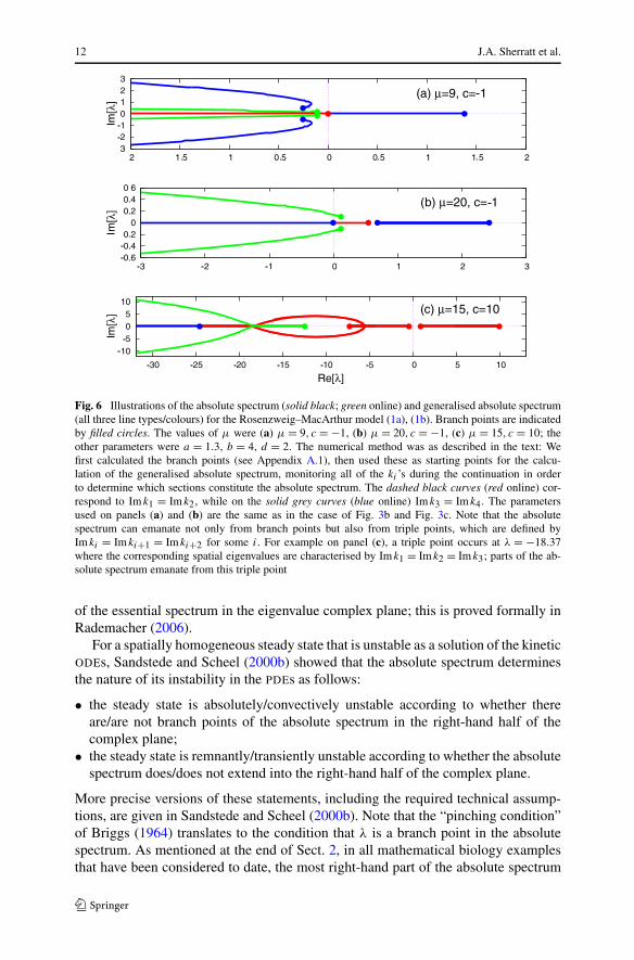
for any i, and this is known as the “generalised absolute spectrum”. This latter set ofeigenvalues was considered (without the name) in the original monograph of Briggs(1964), but the special significance of the case i = n∗ was not realised until Sandstedeand Scheel’s (2000b) work. Two final pieces of terminology are also useful: values ofλ for which kn = kn+1 are known as “branch points of index n”, and “branch pointsin the absolute spectrum” are simply those with index n∗. Figure 6 shows examplesof absolute spectra and generalised absolute spectra. Panels (a) and (b) show theabsolute spectrum and the generalised absolute spectrum for the parameters used inFig. 3b, c.

Note that the absolute spectrum differs from the essential spectrum because thelatter corresponds to both perturbations that grow pointwise and perturbations thatonly grow while simultaneously moving. Thus, the absolute spectrum lies to the left


Fig. 6 Illustrations of the absolute spectrum (solid black; green online) and generalised absolute spectrum(all three line types/colours) for the Rosenzweig–MacArthur model (1a), (1b). Branch points are indicatedby filled circles. The values of μ were (a) μ = 9, c = −1, (b) μ = 20, c = −1, (c) μ = 15, c = 10; theother parameters were a = 1.3, b = 4, d = 2. The numerical method was as described in the text: Wefirst calculated the branch points (see Appendix A.1), then used these as starting points for the calcu-lation of the generalised absolute spectrum, monitoring all of the ki ’s during the continuation in orderto determine which sections constitute the absolute spectrum. The dashed black curves (red online) cor-respond to Im k1 = Imk2, while on the solid grey curves (blue online) Imk3 = Im k4. The parametersused on panels (a) and (b) are the same as in the case of Fig. 3b and Fig. 3c. Note that the absolutespectrum can emanate not only from branch points but also from triple points, which are defined byIm ki = Im ki+1 = Imki+2 for some i. For example on panel (c), a triple point occurs at λ = −18.37where the corresponding spatial eigenvalues are characterised by Imk1 = Im k2 = Im k3; parts of the ab-solute spectrum emanate from this triple point

of the essential spectrum in the eigenvalue complex plane; this is proved formally inRademacher (2006).

For a spatially homogeneous steady state that is unstable as a solution of the kineticODEs, Sandstede and Scheel (2000b) showed that the absolute spectrum determinesthe nature of its instability in the PDEs as follows:

• the steady state is absolutely/convectively unstable according to whether thereare/are not branch points of the absolute spectrum in the right-hand half of thecomplex plane;

• the steady state is remnantly/transiently unstable according to whether the absolutespectrum does/does not extend into the right-hand half of the complex plane.

More precise versions of these statements, including the required technical assump-tions, are given in Sandstede and Scheel (2000b). Note that the “pinching condition”of Briggs (1964) translates to the condition that λ is a branch point in the absolutespectrum. As mentioned at the end of Sect. 2, in all mathematical biology examplesthat have been considered to date, the most right-hand part of the absolute spectrum


is a branch point, so that the notions of absolute and remnant instability, and also ofconvective and transient instability, coincide.

The relationship between the condition Im kn∗ = Im kn∗+1 and these differenttypes of instability is far from obvious. To motivate it intuitively, we present a simpleexample, due originally to Worledge et al. (1997, Sect. 3). We consider a system oftwo coupled reaction–diffusion equations

ut = uxx + f (u, v),

vt = vxx + g(u, v)

on −� < x < �, subject to boundary conditions u = v = 0 at x = ±�, with � large.Here, subscripts x and t denote partial derivatives. For these equations, n∗ = 2 andN = 4. We denote by (us, vs) the homogeneous steady state whose stability is be-ing considered, and write u = u − us , v = v − vs . Then to leading order for smallperturbations u, v,

ut = uxx + fu(us, vs)u + fv(us, vs)v, (3a)

vt = vxx + gu(us, vs)u + gv(us, vs)v, (3b)

where subscripts u and v denote partial derivatives. For a given value of the temporaleigenvalue λ, this has the general solution

(u, v) = eλt

4∑

j=1

(uj , vj )Hj eikj x,

where (uj , vj ) is the eigenvector corresponding to the spatial eigenvalue kj , and theHj ’s are constants. Suppose first that the Im kj ’s are distinct. Then the behaviourof the solution at large positive x is dominated by indices j = 1 and j = 2 in thesummation, so that to leading order for large �, the boundary condition at x = +�

requires

2∑

j=1

(uj , vj )Hj eikj � = (0,0). (4)

Similarly, the boundary condition at x = −� requires

4∑

j=3

(uj , vj )Hj e−ikj � = (0,0) (5)

to leading order. In general, (4) and (5) do not have any non-trivial solutions for theHj ’s. This argument is unaffected if Im k1 = Im k2 and/or Imk3 = Imk4. However, ifIm k2 = Im k3 the situation changes. Then we have

3∑

j=1

(uj , vj )Hj eikj � =

4∑

j=2

(uj , vj )Hj e−ikj � = (0,0)


to leading order, which typically does admit non-trivial solutions for the Hj ’s.Hence, Im k2 = Imk3 is the condition for non-trivial solutions of the linearised equa-tions (3a). Therefore, the extension of the absolute spectrum into the right-hand halfof the complex plane (i.e. a remnant instability) corresponds to the existence of suchnon-trivial solutions for λ > 0, and this is exactly the condition for the steady state tobe unstable on this bounded domain.

Branch points are the key to numerical calculation of the absolute spectrum. SinceD has a repeated root for k at a branch point, we have

D(λ, k) = 0 and (∂/∂k)D(λ, k) = 0. (6)

Now D is a polynomial in both λ and k, and thus it is usually relatively straightfor-ward to solve (6) for the branch points. For example, for (1a), (1b) one can eliminateλ between the two equations in (6) to give a sixth order polynomial in k. This can besolved numerically and then each of the solutions can be substituted back into (6) toget the corresponding values of λ (see Appendix A.1 for further details).

Branch points will be in the absolute spectrum if their index is n∗. To check this fora given branch point, one substitutes the calculated value of λ back into D(λ, k) = 0and solves the resulting polynomial in k. Two of the roots will be the repeated paircorresponding to the branch point. If these are kn∗ and kn∗+1 , then the branch pointis in the absolute spectrum; otherwise it is not.

The above procedure may seem a little involved at first sight, but in practice it isvery straightforward and very quick, involving just the numerical solution of polyno-mials. In the Appendix, we demonstrate the calculation of the branch points for theRosenzweig–MacArthur (1963) model (1a), (1b) and the Klausmeier (1999) model(2a), (2b).

Having calculated the branch points, one can proceed to calculate the entire gen-eralised absolute spectrum via numerical continuation. Using a branch point of in-dex j as a starting point, one performs a numerical continuation of the polynomialD(λ, k), using Rekj −Rekj+1 as a continuation variable. This method was proposedby Rademacher et al. (2007), and it is also described in detail in Smith et al. (2009);the latter paper includes an online supplement with a detailed tutorial guide and sam-ple code. Repeating this procedure for each branch point generates the entire gener-alised absolute spectrum, since for constant coefficient problems all curves of gen-eralised absolute spectrum emanate from a branch point, at least for a wide class ofequations including reaction–diffusion systems (Rademacher et al. 2007). The samestatement does not necessarily hold for the absolute spectrum itself1 and, therefore, itis not possible to calculate the absolute spectrum directly using this approach. Ratherit is necessary to calculate the generalised absolute spectrum, and to monitor all fourroots for k of D(λ, k) = 0 as one moves along it. The absolute spectrum is simply thepart of the generalised absolute spectrum for which Imkn∗ = Im kn∗+1.

In practice, one is interested in the most unstable point in the absolute spec-trum, and also its most unstable branch point. Usually these are the same: This will

1Instead, curves of absolute spectrum can emanate from “triple points”, defined by Im ki = Imki+1 =Im ki+2 for some i (Rademacher et al. 2007; Smith et al. 2009). See Fig. 6c for an example of parts of anabsolute spectrum emanating from triple points.


Fig. 7 An example of stabilityboundaries in the (μ, c) planefor (1a), (1b). The vertical line(dot-dash; solid red online)marks the transition between thecoexistence steady state beingstable and unstable, while thesolid curve (blue online) showsthe transition betweenconvective and absoluteinstability. The latter curve wasplotted via the calculation ofbranch points, as described inAppendix A.1. The parametervalues were a = 1.3, b = 4,d = 2

be the case unless there is a non-transient convective instability (see Sect. 2). Forsome systems, it has been proved that the most unstable point in the absolute spec-trum is a branch point (Smith et al. 2009), but the complexity of most models ofbiological phenomena puts them outside the compass of these results. Therefore,when considering absolute stability in a model for the first time, it is good prac-tice to calculate the full absolute spectrum for a selection of parameter sets; usuallythese will show that the most unstable point in the absolute spectrum is a branchpoint in each case. One can then have confidence in making statements about ab-solute/convective/remnant/transient stability on the basis of branch points, which isusually a very simple calculation. In fact, in the physics literature, where differ-ent types of instability are often considered, many authors draw their conclusionsbased only on calculations of branch points. As an example of a calculation donein this way, Fig. 7 shows the boundary between convective and absolute stabilityof the coexistence steady state in the μ–c plane for (1a), (1b), based simply on nu-merically solving a polynomial to determine the branch points, as described in Ap-pendix A.1.

6 Quantitative Calculations Using Absolute Stability

The example in Sect. 3 illustrates how determination of the type of instability canbe used to understand and predict important qualitative features of spatiotemporalbehaviour. However, the theory is in fact much more powerful than this. Quantita-tive information can also be obtained, by investigating stability in different frames ofreference. We will demonstrate this for the solutions presented in Sect. 3, by adapt-ing the method proposed by Sherratt et al. (2009) for invasions in reaction–diffusionsystems of λ–ω type.

Given a PDE with space variable x and time variable t , one changes to a movingframe of reference in the usual way, by changing coordinates to z = x − V t and t .The frame velocity V is an additional parameter. For any given V , one can use themethods in Sect. 5 to calculate the most unstable point in the absolute spectrum, say


Fig. 8 An example of the dependence of Reλ∗ against V . For a given velocity V , λ∗(V ) is the most un-stable point in the absolute spectrum, meaning that Reλ∗(V ) is the maximum growth rate of perturbationsmoving with velocity V . The example shown is for the Rosenzweig and MacArthur (1963) model (1a),(1b) with parameters a = 1.3, b = 4, c = 0, d = 2, μ = 9. Calculation of the absolute spectrum for thiscase, with a variety of different V values, showed that the most unstable point in the absolute spectrum wasa branch point in all cases. Therefore, we determined λ∗(V ) by calculating branch points, as described inAppendix A.1

λ∗(V ). This is the eigenvalue associated with the most unstable linear mode movingwith velocity V . We denote by k∗ the corresponding value of k. Figure 8 shows atypical plot of Reλ∗ against V , for the model (1a), (1b). There is a finite range ofvelocities for which there are growing linear modes: all linear modes moving withspeed (= |V |) greater than V ∗ are decaying.

A plot such as Fig. 8 is quite instructive in its own right. For example, we pre-sented simulations in Sect. 1 showing that there can be a plateau region behindthe invasion front in which the (unstable) co-existence steady state is “dynami-cally stabilised”. Denoting the invasion velocity by Vfront, the condition for sucha plateau is Vfront > V ∗, so that the invasion can outrun all growing linear modes(Dagbovie and Sherratt 2013). But the curve λ∗(V ) can also form the basis of cal-culations. For example, a natural question arising from the simulations shown inSect. 3 is how the width of the steady state region depends on parameters. To deter-mine this, note that the amplitude of a linear mode travelling with velocity V willdouble over the time period log(2)/Reλ∗(V ). During this time, the linear modemoves a distance V log(2)/Reλ∗(V ) while the transition front moves a distanceVfront log(2)/Reλ∗(V ). Recall that Vfront is the speed of the front, which can be foundusing the theory of minimal spreading speeds (van Saarloos 2003); in the absence of

advection, this speed is given by Vfront0 = 2√

dab

(aμ

μ+1 − 1) but in the context of this

paper, it is defined by Vfront = −Vfront0 −c. Therefore, the linear mode doubles in am-plitude while moving a distance (V −Vfront) log(2)/Reλ∗(V ) from the front. One canreasonably assume that the transition front applies a perturbation to the co-existencesteady state that contains all unstable linear modes. Therefore, the perturbation dou-bles in amplitude over the “doubling distance”

xdbl = log(2)(Vdbl − Vfront)/Reλ∗(Vdbl) (7)


Fig. 9 An illustration of the correlation between the doubling distance xdbl and the width of the steadystate region in simulations of (1a), (1b) with the zero flux condition hx +ch = dpx +cp = 0 at the left-handboundary and the Danckwert condition hx = px = 0 at the right-hand boundary, as in Fig. 5. The parameterμ was varied between 7.9 and 8.5. (a) A plot of xdbl against the numerically calculated width (dots),showing a very strong linear correlation between the two quantities (regression coefficient = 0.999). Thisconfirms that the dependence on parameters of the width of the steady state region is captured by xdbl . Theline is the best-fit regression line, which has slope 98.05 and intercept 5.795; there is a non-zero interceptbecause our method for measuring the width of the steady-state region excludes small portions on eitherside (see Smith and Sherratt 2009 for further discussion). (b) A plot of the width of the steady state region(dots) against μ. We superimpose on this a curve showing xdbl , rescaled using the regression line foundfrom (a). The doubling distance was calculated using (7) and (8). The width of the steady state region wascalculated using numerical simulations performed as in Fig. 5; the space and time discretisations are asin Fig. 1. The method used to measure the width in numerical simulations is described in Dagbovie andSherratt (2013). The parameter values were a = 1.3, b = 4, c = −0.5, d = 2

where Vdlb minimises (V − Vfront)/Reλ∗(V ), i.e.

(Vdbl − Vfront)d

dVReλ∗(V )

∣

∣

∣

∣

V =Vdbl

= Reλ∗(Vdbl). (8)

Numerical solution of (8) is made relatively straightforward by the identity(d/dV )Reλ∗(V )|V =Vdbl

= − Imk∗(Vdbl) (Sherratt et al. 2009). In some cases,(8) will have more than one solution: Then the relevant solution is the one givingthe smallest value of xdbl ; an example of this is given in Fig. 5 of Smith and Sher-ratt (2009). The formula (7) for xdbl contains all of the parameter dependence of thewidth of the steady state region in the simulations shown in Sect. 3. For example,Fig. 9 plots xdbl against estimates of the width from simulations as the parameter μ

is varied, demonstrating their linear relationship.

7 Summary and Discussion

Biology abounds with complex spatiotemporal phenomena. Mathematical modelshave been highly successful at reproducing this complexity, but currently our abil-ity to numerically simulate such phenomena far outstrips our ability to provide anunderlying mathematical understanding. As a result, models can sometimes fail tofulfil their potential for qualitative and quantitative prediction. The theory of absolutestability provides a tool that has the potential to redress this inbalance in some cases,and whose use within mathematical biology is currently almost non-existent. Untilrecently, one had to overcome a steep learning curve to make practical use of thistheory, but new computational methods based on the absolute spectrum now make it


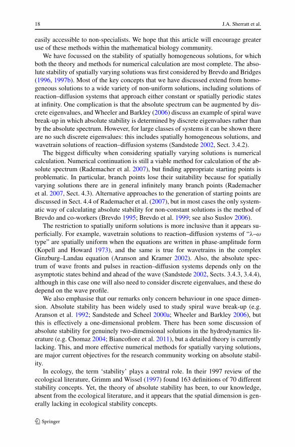
easily accessible to non-specialists. We hope that this article will encourage greateruse of these methods within the mathematical biology community.

We have focussed on the stability of spatially homogeneous solutions, for whichboth the theory and methods for numerical calculation are most complete. The abso-lute stability of spatially varying solutions was first considered by Brevdo and Bridges(1996, 1997b). Most of the key concepts that we have discussed extend from homo-geneous solutions to a wide variety of non-uniform solutions, including solutions ofreaction–diffusion systems that approach either constant or spatially periodic statesat infinity. One complication is that the absolute spectrum can be augmented by dis-crete eigenvalues, and Wheeler and Barkley (2006) discuss an example of spiral wavebreak-up in which absolute stability is determined by discrete eigenvalues rather thanby the absolute spectrum. However, for large classes of systems it can be shown thereare no such discrete eigenvalues: this includes spatially homogeneous solutions, andwavetrain solutions of reaction–diffusion systems (Sandstede 2002, Sect. 3.4.2).

The biggest difficulty when considering spatially varying solutions is numericalcalculation. Numerical continuation is still a viable method for calculation of the ab-solute spectrum (Rademacher et al. 2007), but finding appropriate starting points isproblematic. In particular, branch points lose their suitability because for spatiallyvarying solutions there are in general infinitely many branch points (Rademacheret al. 2007, Sect. 4.3). Alternative approaches to the generation of starting points arediscussed in Sect. 4.4 of Rademacher et al. (2007), but in most cases the only system-atic way of calculating absolute stability for non-constant solutions is the method ofBrevdo and co-workers (Brevdo 1995; Brevdo et al. 1999; see also Suslov 2006).

The restriction to spatially uniform solutions is more inclusive than it appears su-perficially. For example, wavetrain solutions to reaction–diffusion systems of “λ–ω

type” are spatially uniform when the equations are written in phase-amplitude form(Kopell and Howard 1973), and the same is true for wavetrains in the complexGinzburg–Landau equation (Aranson and Kramer 2002). Also, the absolute spec-trum of wave fronts and pulses in reaction–diffusion systems depends only on theasymptotic states behind and ahead of the wave (Sandstede 2002, Sects. 3.4.3, 3.4.4),although in this case one will also need to consider discrete eigenvalues, and these dodepend on the wave profile.

We also emphasise that our remarks only concern behaviour in one space dimen-sion. Absolute stability has been widely used to study spiral wave break-up (e.g.Aranson et al. 1992; Sandstede and Scheel 2000a; Wheeler and Barkley 2006), butthis is effectively a one-dimensional problem. There has been some discussion ofabsolute stability for genuinely two-dimensional solutions in the hydrodynamics lit-erature (e.g. Chomaz 2004; Biancofiore et al. 2011), but a detailed theory is currentlylacking. This, and more effective numerical methods for spatially varying solutions,are major current objectives for the research community working on absolute stabil-ity.

In ecology, the term ‘stability’ plays a central role. In their 1997 review of theecological literature, Grimm and Wissel (1997) found 163 definitions of 70 differentstability concepts. Yet, the theory of absolute stability has been, to our knowledge,absent from the ecological literature, and it appears that the spatial dimension is gen-erally lacking in ecological stability concepts.


This is particularly surprising since stream ecologists (and water resource man-agers alike) have long been on the quest of how lotic systems respond to disturbancesand spatial variabilities. Much of the current knowledge comes from experimentsin study sites that comprise only a small fragment of the stream or river (Fauschet al. 2002). But how do populations much further downstream, i.e. outside the studyarena, respond to upstream perturbations (Cooper et al. 1998)? This is a key questionin the assessment of instream flow needs, or how the location of wastewater treatmentplants affects environmental conditions downstream (Anderson et al. 2006). One at-tempt to address this question is the concept of the response length (Anderson et al.2005), a characteristic length scale measuring the scale over which environmentaldisturbances are felt by distant populations.

Convective instabilities appear particularly intriguing in this context. The per-turbed steady state remains stable locally, but is enormously brought out of equi-librium further downstream (cf. Fig. 5b). Small-scale experiments and observationsmight only see the local (stable) response, but miss out on the instabilities arisingfurther away. In Sect. 6, we have shown how the width of the region where the steadystate remains stable can be calculated quantitatively (see also Dagbovie and Sher-ratt 2013). This may be useful information for the design of experiments, ecologicalmonitoring as well as environmental assessment.

The convective and absolute instabilities that we have described do not necessarilyneed to be ‘harmful’ to the populations. On the contrary, the spatiotemporal oscilla-tions caused by the instabilities can be beneficial. For example, they might facili-tate non-equilibrium coexistence of species that would otherwise mutually excludeeach other (Armstrong and McGehee 1980; Huisman and Weissing 1999). In a morewater-flow oriented context, Scheuring et al. (2000) have shown that the chaotic flowaround a cylindrical obstacle creates a small-scale mosaic ensuring that coexistingspecies can co-exist. Similarly, Lee (2012) has argued that rotational flow, as causedby a rock, can increase survival probabilities of predators and prey. Petrovskii et al.(2004) have shown, in a non-advective model that spatiotemporal chaos can reversethe paradox of enrichment, and thus make the persistence of predators and prey morelikely.

Convective and absolute instabilities can lead to spatial and spatiotemporal pat-terns. Many of the well-known mechanisms inducing biological pattern formationare based on the phenomenon that steady states which are locally stable in thekinetic ODEs become destabilised in the PDEs. For instance, the diffusion-driveninstabilities of the Turing mechanism are caused by the addition of significantlydifferent diffusivities, which lead to short-range activation and long-range inhibi-tion. Advective environments feature a number of spatiotemporal pattern formationmechanisms that cannot arise in non-advective systems. In contrast to the Turingmechanism, they do not require activator–inhibitor type of interactions, but theycritically depend on other conditions, e.g. a significant difference in the flow ex-perienced by species (Rovinsky and Menzinger 1992; Perumpanani et al. 1995;Malchow 2000) or resource-dependent dispersal (Anderson et al. 2012). However,they all have in common that the steady states in the kinetic ODEs are locally stable.

The patterns generated by convective and absolute instabilities do not require anyof these conditions (activator–inhibitor dynamics; significantly different mobilities


of the interacting species; resource-dependent dispersal). However, in contrast to thepreviously mentioned mechanisms, the steady states are already unstable in the ki-netic ODEs. Considering the abundance of endogenous population oscillations, thisis frequently the case in nature and can be caused by a number of mechanisms (seeTurchin 2003). Hence, convective and absolute instabilities appear to be a fairly gen-eral mechanism for spatiotemporal pattern formation in ecology.

Streams and river are particularly iconic examples of flow-dominated systems, butthere are many others. Marine organisms dispersed in longshore currents (Gaylordand Gaines 2000) or plant seeds and insects dispersed by winds with a prevailingwind direction (Levine 2003) are also environments with a predominantly unidirec-tional flow. These systems are strongly characterised by the importance of longitudi-nal transport through habitat. The theory of absolute stability appears to have a lot tooffer when there is a downstream bias that can induce very different spatial responsesto localised perturbations.

Acknowledgements J.A.S. acknowledges discussions with Leonid Brevdo (Louis Pasteur University,Strasbourg), Jens Rademacher (CWI, Amsterdam), Björn Sandstede (Brown University) and MatthewSmith (Microsoft Research, Cambridge). A.S.D. was supported by the Centre for Analysis and NonlinearPDEs funded by the UK EPSRC grant EP/E03635X and the Scottish Funding Council. F.M.H. acknowl-edges discussions with Mark Lewis (University of Alberta), Sergei Petrovskii (University of Leicester) andFrithjof Lutscher (University of Ottawa).

Appendix: Examples of Calculating Branch Points

In this Appendix, we show how to calculate the branch points for the Rosenzweig–MacArthur model (1a), (1b) and the Klausmeier model (2a), (2b). We present thesecalculations in some detail, with the aim of providing templates that readers can fol-low when performing corresponding calculations for their own models.

A.1 Branch Points for the Rosenzweig–MacArthur Model

Recall that the Rosenzweig–MacArthur model (1a), (1b) has a unique homogeneousco-existence steady state (hs,ps) where hs = 1/(aμ − μ) and ps = (1 − hs)(1 +μhs)/μ. We begin by linearising (1a), (1b) about (hs,ps) giving

pt = αp + βh + cpx + dpxx,

ht = γ p + δh + chx + hxx,

where p = p −ps , h = h−hs , and α, β, γ, δ are coefficients from linearisation andare given by

α = μhs

b(1 + μhs)− 1

ab,

β = μps

b(1 + μhs)2,

γ = 1 − 2hs − μps

(1 + μhs)2,


δ = − μhs

1 + μhs

.

Substituting (p, h) = (p, h) exp(ikx +λt) into (1a), (1b) and requiring p and h to benon-zero gives the dispersion relation

D(λ, k) = dk4 − cik3(d + 1) − k2(α − λ + dγ − dλ + c2)

+ cik(γ + α − 2λ) + (α − λ)(γ − λ) − δβ = 0. (9)

Branch points are double roots of the dispersion relation for k, and satisfy (9) andalso

0 = ∂D/∂k

= 4dk3 − 3k2(1 + d)ci − 2k(

γ + dα − (1 + d)λ) + c2 + ci(α + γ − 2λ) ⇒

λ = 4dk3 − 3cidk2 − 2dkγ + αci − 2c2k − 3cik2 − 2αk + ciγ

−2(k + dk − ci).

(10)Substituting (10) into (9) gives the following hexic polynomial in k:

[−4d(d − 1)2]k6 + [

2ci(d + 1)(d − 1)2]k5 + [

(d − 1)(

c2d + 8dα − 8dγ − c2)]k4

+ [

4ci(−α + γ )(d − 1)(d + 1)]

k3

+ [

2c2(d − 1)(γ − α) − 4βδ(d + 1)2 − 4d(α − γ )2]k2

+ [

2i(

4βδ + α2 − 2αγ + γ 2)c(d + 1)]

k + c2(4βδ + α2 − 2αγ + γ 2) = 0.

(11)

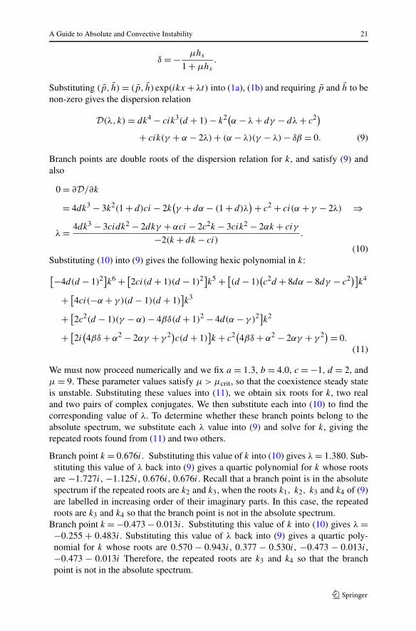
We must now proceed numerically and we fix a = 1.3, b = 4.0, c = −1, d = 2, andμ = 9. These parameter values satisfy μ > μcrit, so that the coexistence steady stateis unstable. Substituting these values into (11), we obtain six roots for k, two realand two pairs of complex conjugates. We then substitute each into (10) to find thecorresponding value of λ. To determine whether these branch points belong to theabsolute spectrum, we substitute each λ value into (9) and solve for k, giving therepeated roots found from (11) and two others.

Branch point k = 0.676i. Substituting this value of k into (10) gives λ = 1.380. Sub-stituting this value of λ back into (9) gives a quartic polynomial for k whose rootsare −1.727i, −1.125i, 0.676i, 0.676i. Recall that a branch point is in the absolutespectrum if the repeated roots are k2 and k3, when the roots k1, k2, k3 and k4 of (9)are labelled in increasing order of their imaginary parts. In this case, the repeatedroots are k3 and k4 so that the branch point is not in the absolute spectrum.

Branch point k = −0.473 − 0.013i. Substituting this value of k into (10) gives λ =−0.255 + 0.483i. Substituting this value of λ back into (9) gives a quartic poly-nomial for k whose roots are 0.570 − 0.943i, 0.377 − 0.530i, −0.473 − 0.013i,−0.473 − 0.013i Therefore, the repeated roots are k3 and k4 so that the branchpoint is not in the absolute spectrum.


Branch point k = 0.473 − 0.013i. Substituting this value of k into (10) gives λ =−0.255 − 0.483i. Substituting this value of λ back into (9) gives a quartic poly-nomial for k whose roots are −0.570 − 0.943i, −0.377 − 0.530i, 0.473 − 0.013i,0.473 − 0.013i. Therefore, the repeated roots are k3 and k4 so that the branch pointis not in the absolute spectrum.

Branch point k = 0.001 − 0.334i. Substituting this value of k into (10) gives λ =−0.110 − 0.167i. Substituting this value of λ back into (9) gives a quartic poly-nomial for k whose roots are −0.314 − 0.816i, 0.001 − 0.334i, 0.001 − 0.334i,0.312−0.0165i. Therefore, the repeated roots are k2 and k3 so that the branch pointis in the absolute spectrum.

Branch point k = −0.001 − 0.334i. Substituting this value of k into (10) gives λ =−0.110 + 0.167i. Substituting this value of λ back into (9) gives a quartic poly-nomial for k whose roots are 0.314 − 0.816i, −0.001 − 0.334i, −0.001 − 0.334i,−0.312 − 0.0165i. Therefore, the repeated roots are k2 and k3 so that the branchpoint is in the absolute spectrum.

Branch point k = −0.732i. Substituting this value of k into (10) gives λ = 0.000.Substituting this value of λ back into (9) gives a quartic polynomial for k whoseroots are −0.732i, −0.732i, 0.160 − 0.017i, −0.160 − 0.017i. Therefore, the re-peated roots are k1 and k2 so that the branch point is not in the absolute spectrum.

Therefore, of the six branch points, two are in the absolute spectrum, with the corre-sponding eigenvalues being −0.110 ± 0.167i. Since these eigenvalues have negativereal parts, the steady state (hs,ps) is absolutely stable. To determine whether theconvective instability is of transient or remnant type, it is necessary to calculate theabsolute spectrum. This can be done via numerical continuation of the generalisedabsolute spectrum, using the six branch points listed above as starting points, as dis-cussed in Sect. 5. This shows that the branch points are the most unstable points inthe absolute spectrum, so that the steady state has a transient convective instability.

A.2 Branch Points for the Klausmeier Model

For all parameters, the Klausmeier model (2a), (2b) has a “desert” steady state m = 0,w = A. When A ≥ 2B , there are two further steady states (m±,w±) where

m± = 2B

A ± √A2 − 4B2

, w± = A ± √A2 − 4B2

2.

Ecologically realistic values of B are relatively small, and in particular satisfy B < 2(Klausmeier 1999; Rietkerk et al. 2002). Under this constraint, (m−,w−) is stableas a solution of the kinetics ODEs, although it can be destabilised by the diffusionand advection terms, leading to spatial patterns (Klausmeier 1999; Sherratt 2005,2010). However, (m+,w+) is unstable as a solution of the kinetic ODEs, and we willconsider the nature of its instability as a solution of the PDEs (2a), (2b).

We begin by linearising (2a), (2b) about (m+,w+), giving

mt = αm + βw + mxx, (12a)

wt = γ m + δw + νwx, (12b)


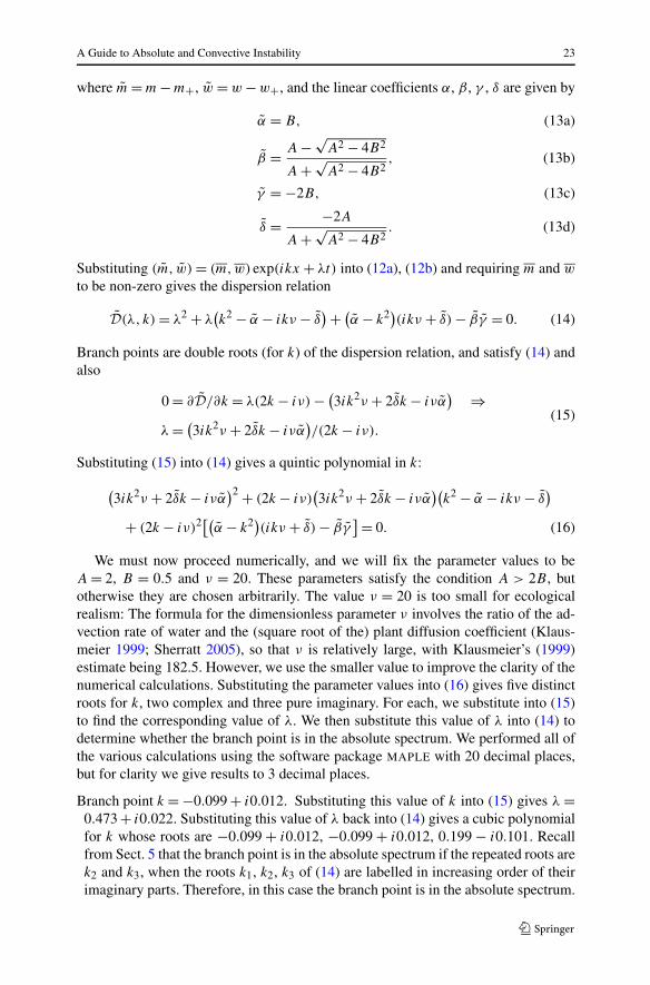
where m = m − m+, w = w − w+, and the linear coefficients α, β , γ , δ are given by

α = B, (13a)

β = A − √A2 − 4B2

A + √A2 − 4B2

, (13b)

γ = −2B, (13c)

δ = −2A

A + √A2 − 4B2

. (13d)

Substituting (m, w) = (m,w) exp(ikx + λt) into (12a), (12b) and requiring m and w

to be non-zero gives the dispersion relation

D(λ, k) = λ2 + λ(

k2 − α − ikν − δ) + (

α − k2)(ikν + δ) − βγ = 0. (14)

Branch points are double roots (for k) of the dispersion relation, and satisfy (14) andalso

0 = ∂D/∂k = λ(2k − iν) − (

3ik2ν + 2δk − iνα) ⇒

λ = (

3ik2ν + 2δk − iνα)

/(2k − iν).(15)

Substituting (15) into (14) gives a quintic polynomial in k:

(

3ik2ν + 2δk − iνα)2 + (2k − iν)

(

3ik2ν + 2δk − iνα)(

k2 − α − ikν − δ)

+ (2k − iν)2[(α − k2)(ikν + δ) − βγ] = 0. (16)

We must now proceed numerically, and we will fix the parameter values to beA = 2, B = 0.5 and ν = 20. These parameters satisfy the condition A > 2B , butotherwise they are chosen arbitrarily. The value ν = 20 is too small for ecologicalrealism: The formula for the dimensionless parameter ν involves the ratio of the ad-vection rate of water and the (square root of the) plant diffusion coefficient (Klaus-meier 1999; Sherratt 2005), so that ν is relatively large, with Klausmeier’s (1999)estimate being 182.5. However, we use the smaller value to improve the clarity of thenumerical calculations. Substituting the parameter values into (16) gives five distinctroots for k, two complex and three pure imaginary. For each, we substitute into (15)to find the corresponding value of λ. We then substitute this value of λ into (14) todetermine whether the branch point is in the absolute spectrum. We performed all ofthe various calculations using the software package MAPLE with 20 decimal places,but for clarity we give results to 3 decimal places.

Branch point k = −0.099 + i0.012. Substituting this value of k into (15) gives λ =0.473 + i0.022. Substituting this value of λ back into (14) gives a cubic polynomialfor k whose roots are −0.099 + i0.012, −0.099 + i0.012, 0.199 − i0.101. Recallfrom Sect. 5 that the branch point is in the absolute spectrum if the repeated roots arek2 and k3, when the roots k1, k2, k3 of (14) are labelled in increasing order of theirimaginary parts. Therefore, in this case the branch point is in the absolute spectrum.


Branch point k = −i19.950. Substituting this value of k into (15) gives λ = 398.112.Substituting this value of λ back into (14) gives a cubic polynomial for k whose rootsare −i19.950, −i19.950 and i19.94. Therefore, the repeated roots are k1 and k2, sothat this branch point is not in the absolute spectrum.

Branch point k = −i19.892. Substituting this value of k into (15) gives λ = 396.587.Substituting this value of λ back into (14) gives a cubic polynomial for k whose rootsare −i19.892, −i19.892 and i19.902. Therefore, the repeated roots are k1 and k2,so that this branch point is not in the absolute spectrum.

Branch point k = −i0.181. Substituting this value of k into (15) gives λ = 0.569.Substituting this value of λ back into (14) gives a cubic polynomial for k whoseroots are −i0.181, −i0.181, and i0.281. Therefore, the repeated roots are k1 andk2, so that this branch point is not in the absolute spectrum.

Branch point k = 0.099 + i0.012. Substituting this value of k into (15) gives λ =0.473 − i0.022. Substituting this value of λ back into (14) gives a cubic polynomialfor k whose roots are −0.199 − i0.101, 0.099 + i0.012, and 0.099 + i0.012. There-fore, the repeated roots are k2 and k3, so that this branch point is in the absolutespectrum.

Therefore, of the five branch points, two are in the absolute spectrum, with the cor-responding eigenvalues being 0.473 ± i0.022. Since these eigenvalues have positivereal part, the steady state (m+,w+) is absolutely unstable.

References

Anderson, K. E., Nisbet, R. M., Diehl, S., & Cooper, S. D. (2005). Scaling population responses to spatialenvironmental variability in advection-dominated systems. Ecol. Lett., 8, 933–943.

Anderson, K. E., Paul, A. J., McCauley, E., Jackson, L. J., Post, J. R., & Nisbet, R. M. (2006). Instreamflow needs in streams and rivers: the importance of understanding ecological dynamics. Front. Ecol.Environ., 4, 309–318.

Anderson, K. E., Hilker, F. M., & Nisbet, R. M. (2012). Directional dispersal and emigration behaviordrive a flow-induced instability in a stream consumer-resource model. Ecol. Lett., 15, 209–217.

Aranson, I. S., & Kramer, L. (2002). The world of the complex Ginzburg–Landau equation. Rev. Mod.Phys., 74, 99–143.

Aranson, I. S., Aranson, L., Kramer, L., & Weber, A. (1992). Stability limits of spirals and traveling wavesin nonequilibrium media. Phys. Rev. A, 46, R2992–R2995.

Armstrong, R. A., & McGehee, R. (1980). Competitive exclusion. Am. Nat., 115, 151–170.Beyn, W.-J., & Lorenz, J. (1999). Stability of travelling waves: dichotomies and eigenvalue conditions on

finite intervals. Numer. Funct. Anal. Optim., 20, 201–244.Biancofiore, L., Gallaire, F., & Pasquetti, R. (2011). Influence of confinement on a two-dimensional wake.

J. Fluid Mech., 688, 297–320.Brandt, M. J., & Lambin, X. (2007). Movement patterns of a specialist predator, the weasel Mustela nivalis

exploiting asynchronous cyclic field vole Microtus agrestis populations. Acta Theriol., 52, 13–25.Brevdo, L. (1988). A study of absolute and convective instabilities with an application to the Eady model.

Geophys. Astrophys. Fluid Dyn., 40, 1–92.Brevdo, L. (1995). Convectively unstable wave packets in the Blasius boundary layer. Z. Angew. Math.

Mech., 75, 423–436.Brevdo, L., & Bridges, T. J. (1996). Absolute and convective instabilities of spatially periodic flows. Philos.

Trans. R. Soc. Lond. A, 354, 1027–1064.Brevdo, L., & Bridges, T. J. (1997a). Absolute and convective instabilities of temporally oscillating flows.

Z. Angew. Math. Phys., 48, 290–309.Brevdo, L., & Bridges, T. J. (1997b). Local and global instabilities of spatially developing flows: cautionary

examples. Proc. R. Soc. Lond. A, 453, 1345–1364.


Brevdo, L., Laure, P., Dias, F., & Bridges, T. J. (1999). Linear pulse structure and signalling in a film flowon an inclined plane. J. Fluid Mech., 396, 37–71.

Briggs, R. J. (1964). Electron-stream interaction with plasmas. Cambridge: MIT Press.Chomaz, J. M. (2004). Transition to turbulence in open flows: what linear and fully nonlinear local and

global theories tell us. Eur. J. Mech. B, 23, 385–399.Chomaz, J. M. (2005). Global instabilities in spatially developing flows: non-normality and nonlinearity.

Annu. Rev. Fluid Mech., 37, 357–392.Cooper, S. D., Diehl, S., Kratz, K., & Sarnelle, O. (1998). Implications of scale for patterns and processes

in stream ecology. Aust. J. Ecol., 23, 27–40.Dagbovie, A. S., & Sherratt, J. A. (2013, accepted). Absolute stability and dynamical stabilisation in

predator–prey systems. J. Math. Biol. doi:10.1007/s00285-013-0672-8.Dunbar, S. R. (1986). Traveling waves in diffusive predator–prey equations—periodic orbits and point-to-

periodic heteroclinic orbits. SIAM J. Appl. Math., 46, 1057–1078.Fausch, K. D., Torgersen, C. E., Baxter, C. V., & Li, H. W. (2002). Landscapes to riverscapes: bridging the

gap between research and conservation of stream fishes. Bioscience, 52, 483–498.Fox, P. J., & Proctor, M. R. E. (1998). Effects of distant boundaries on pattern forming instabilities. Phys.

Rev. E, 57, 491–494.Fraile, J. M., & Sabina, J. C. (1989). General conditions for the existence of a critical point–periodic wave

front connection for reaction–diffusion systems. Nonlinear Anal.-Theor., 13, 767–786.Gaylord, B., & Gaines, S. D. (2000). Temperature or transport? Range limits in marine species mediated

solely by flow. Am. Nat., 155, 769–789.Grimm, V., & Wissel, C. (1997). Babel, or the ecological stability discussions: an inventory and analysis

of terminology and a guide for avoiding confusion. Oecologia, 109, 323–334.Hauzy, C., Hulot, F. D., & Gins, A. (2007). Intra and interspecific density-dependent dispersal in an aquatic

prey–predator system. J. Anim. Ecol., 76, 552–558.Hilker, F. M., & Lewis, M. A. (2010). Predator-prey systems in streams and rivers. Theor. Ecol., 3, 175–

193.Huerre, P., & Monkewitz, P. A. (1990). Local and global instabilities in spatially developing flows. Annu.

Rev. Fluid Mech., 22, 473–537.Huisman, J., & Weissing, F. J. (1999). Biodiversity of plankton by species oscillations and chaos. Nature,

402, 407–410.Klausmeier, C. A. (1999). Regular and irregular patterns in semiarid vegetation. Science, 284, 1826–1828.Kopell, N., & Howard, L. N. (1973). Plane wave solutions to reaction–diffusion equations. Stud. Appl.

Math., 52, 291–328.Lee, S.-H. (2012). Effects of uniform rotational flow on predator–prey system. Physica A, 391, 6008–6015.Levine, J. M. (2003). A patch modeling approach to the community-level consequences of directional

dispersal. Ecology, 84, 1215–1224.Lutscher, F., Lewis, M. A., & McCauley, E. (2006). Effects of heterogeneity on spread and persistence in

rivers. Bull. Math. Biol., 68, 2129–2160.Malchow, H. (2000). Motional instabilities in predator–prey systems. J. Theor. Biol., 204, 639–647.Malchow, H., & Petrovskii, S. V. (2002). Dynamical stabilization of an unstable equilibrium in chemical

and biological systems. Math. Comput. Model., 36, 307–319.Merchant, S. M., & Nagata, W. (2010). Wave train selection behind invasion fronts in reaction–diffusion

predator–prey models. Physica D, 239, 1670–1680.Merchant, S. M., & Nagata, W. (2011). Instabilities and spatiotemporal patterns behind predator invasions

with nonlocal prey competition. Theor. Popul. Biol., 80, 289–297.Morozov, A. Yu., Petrovskii, S. V, & Li, B.-L. (2006). Spatiotemporal complexity of the patchy invasion

in a predator–prey system with the Allee effect. J. Theor. Biol., 238, 18–35.Nauman, E. B. (2008). Chemical reactor design, optimization, and scaleup (2nd ed.). Hoboken: Wiley.Owen, M. R., & Lewis, M. A. (2001). How predation can slow, stop or reverse a prey invasion. Bull. Math.

Biol., 63, 655–684.Perumpanani, A. J., Sherratt, J. A., & Maini, P. K. (1995). Phase differences in reaction–diffusion–

advection systems and applications to morphogenesis. IMA J. Appl. Math., 55, 19–33.Petrovskii, S. V., & Malchow, H. (2000). Critical phenomena in plankton communities: KISS model revis-

ited. Nonlinear Anal., Real World Appl., 1, 37–51.Petrovskii, S., Li, B.-L., & Malchow, H. (2004). Transition to spatiotemporal chaos can resolve the paradox

of enrichment. Ecol. Complex., 1, 37–47.Rademacher, J. D. M. (2006). Geometric relations of absolute and essential spectra of wave trains. SIAM

J. Appl. Dyn. Syst., 5, 634–649.

http://dx.doi.org/10.1007/s00285-013-0672-8


Rademacher, J. D. M., Sandstede, B., & Scheel, A. (2007). Computing absolute and essential spectra usingcontinuation. Physica D, 229, 166–183.

Rietkerk, M., Boerlijst, M. C., van Langevelde, F., HilleRisLambers, R., van de Koppel, J., Prins, H. H. T.,& de Roos, A. (2002). Self-organisation of vegetation in arid ecosystems. Am. Nat., 160, 524–530.

Rosenzweig, M. L., & MacArthur, R. H. (1963). Graphical representation and stability conditions ofpredator–prey interactions. Am. Nat., 97, 209–223.

Rovinsky, A. B., & Menzinger, M. (1992). Chemical instability induced by a differential flow. Phys. Rev.Lett., 69, 1193–1196.

Sandstede, B. (2002). Stability of travelling waves. In B. Fiedler (Ed.), Handbook of dynamical systems II(pp. 983–1055). Amsterdam: North-Holland.

Sandstede, B., & Scheel, A. (2000a). Absolute versus convective instability of spiral waves. Phys. Rev. E,62, 7708–7714.

Sandstede, B., & Scheel, A. (2000b). Absolute and convective instabilities of waves on unbounded andlarge bounded domains. Physica D, 145, 233–277.

Scheuring, I., Károlyi, G., Péntek, A., Tel, T., & Toroczkai, Z. (2000). A model for resolving the planktonparadox: coexistence in open flows. Freshw. Biol., 45, 123–132.

Sherratt, J. A. (2005). An analysis of vegetation stripe formation in semi-arid landscapes. J. Math. Biol.,51, 183–197.

Sherratt, J. A. (2010). Pattern solutions of the Klausmeier model for banded vegetation in semi-arid envi-ronments I. Nonlinearity, 23, 2657–2675.

Sherratt, J. A., Lewis, M. A., & Fowler, A. C. (1995). Ecological chaos in the wake of invasion. Proc. Natl.Acad. Sci. USA, 92, 2524–2528.

Sherratt, J. A., Smith, M. J., & Rademacher, J. D. M. (2009). Locating the transition from periodic oscilla-tions to spatiotemporal chaos in the wake of invasion. Proc. Natl. Acad. Sci. USA, 106, 10890–10895.

Smith, M. J., & Sherratt, J. A. (2009). Propagating fronts in the complex Ginzburg–Landau equationgenerate fixed-width bands of plane waves. Phys. Rev. E, 80, 046209.

Smith, M. J., Sherratt, J. A., & Lambin, X. (2008). The effects of density-dependent dispersal on thespatiotemporal dynamics of cyclic populations. J. Theor. Biol., 254, 264–274.

Smith, M. J., Rademacher, J. D. M., & Sherratt, J. A. (2009). Absolute stability of wavetrains can explainspatiotemporal dynamics in reaction–diffusion systems of lambda–omega type. SIAM J. Appl. Dyn.Syst., 8, 1136–1159.

Suslov, S. A. (2001). Searching convective/absolute instability boundary for flows with fully numericaldispersion relation. Comput. Phys. Commun., 142, 322–325.

Suslov, S. A. (2006). Numerical aspects of searching convective/absolute instability transition. J. Comp.Physiol., 212, 188–217.

Suslov, S. A. (2009). Analysis of instability patterns in non-Boussinesq mixed convection using a directnumerical evaluation of disturbance integrals. Comput. Fluids, 38, 590–601.

Suslov, S. A., & Paolucci, S. (2004). Stability of non-Boussinesq convection via the complex Ginzburg–Landau model. Fluid Dyn. Res., 35, 159–203.

Tobias, S. M., Proctor, M. R. E., & Knobloch, E. (1998). Convective and absolute instabilities of fluidflows in finite geometries. Physica D, 113, 43–72.

Turchin, P. (2003). Complex population dynamics. A Theoretical/Empirical synthesis. Princeton: PrincetonUniversity Press.

van Saarloos, W. (2003). Front propagation into unstable states. Phys. Rep., 386, 29–222.Wheeler, P., & Barkley, D. (2006). Computation of spiral spectra. SIAM J. Appl. Dyn. Syst., 5, 157–177.Wieters, E. A., Gaines, S. D., Navarrete, S. A., Blanchette, C. A., & Menge, B. A. (2008). Scales of

dispersal and the biogeography of marine predator–prey interactions. Am. Nat., 171, 405–417.Worledge, D., Knobloch, E., Tobias, S., & Proctor, M. (1997). Dynamo waves in semi-infinite and finite

domains. Proc. R. Soc. Lond. A, 453, 119–143.

a mathematical biologist’s guide to absolute and

Documents